University of Adelaide, June 2010 - School of Economics · Regression Techniques in Stata...

Regression Techniques in Stata

Christopher F Baum

Boston College and DIW Berlin

University of Adelaide, June 2010

Christopher F Baum (BC / DIW) Regression Techniques in Stata Adelaide, June 2010 1 / 134

Basics of Regression with Stata


A key tool in multivariate statistical inference is linear regression, inwhich we specify the conditional mean of a response variable y as alinear function of k independent variables

E [y |x1, x2, . . . , xk ] = β1x1 + β2x2 + · · ·+ βkxi,k (1)

Note that the conditional mean of y is a function of x1, x2, . . . , xk withfixed parameters β1, β2, . . . , βk . Given values for these βs the linearregression model predicts the average value of y in the population fordifferent values of x1, x2, . . . , xk .



For example, suppose that the mean value of single-family homeprices in Boston-area communities, conditional on the communities’student-teacher ratios, is given by

E [p | stratio] = β1 + β2 stratio (2)

This relationship reflects the hypothesis that the quality ofcommunities’ school systems is capitalized into the price of housing ineach community. In this example the population is the set ofcommunities in the Commonwealth of Massachusetts. Each town orcity in Massachusetts is generally responsible for its own schoolsystem.



Conditional mean of housing price:0

1000

020

000

3000

040

000

12 14 16 18 20 22Student−teacher ratio

Average single−family house price



We display average single-family housing prices for 100 Boston-areacommunities, along with the linear fit of housing prices to communities’student-teacher ratios. The conditional mean of p, price, for each valueof stratio, the student-teacher ratio is given by the appropriate point onthe line. As theory predicts, the mean house price conditional on thecommunity’s student-teacher ratio is inversely related to that ratio.Communities with more crowded schools are considered lessdesirable. Of course, this relationship between house price and thestudent-teacher ratio must be considered ceteris paribus: all otherfactors that might affect the price of the house are held constant whenwe evaluate the effect of a measure of community schools’ quality onthe house price.



This population regression function specifies that a set of k regressorsin X and the stochastic disturbance u are the determinants of theresponse variable (or regressand) y . The model is usually assumed tocontain a constant term, so that x1 is understood to equal one for eachobservation. We may write the linear regression model in matrix formas

y = Xβ + u (3)

where X = x1, x2, . . . , xk, an N × k matrix of sample values.



The key assumption in the linear regression model involves therelationship in the population between the regressors X and u. Wemay rewrite Equation (3) as

u = y − Xβ (4)

We assume thatE (u | X ) = 0 (5)

i.e., that the u process has a zero conditional mean. This assumptionstates that the unobserved factors involved in the regression functionare not related in any systematic manner to the observed factors. Thisapproach to the regression model allows us to consider bothnon-stochastic and stochastic regressors in X without distinction; allthat matters is that they satisfy the assumption of Equation (5).


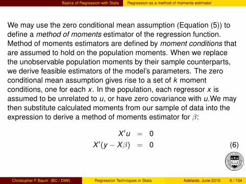
Basics of Regression with Stata Regression as a method of moments estimator

We may use the zero conditional mean assumption (Equation (5)) todefine a method of moments estimator of the regression function.Method of moments estimators are defined by moment conditions thatare assumed to hold on the population moments. When we replacethe unobservable population moments by their sample counterparts,we derive feasible estimators of the model’s parameters. The zeroconditional mean assumption gives rise to a set of k momentconditions, one for each x . In the population, each regressor x isassumed to be unrelated to u, or have zero covariance with u.We maythen substitute calculated moments from our sample of data into theexpression to derive a method of moments estimator for β:

X ′u = 0X ′(y − Xβ) = 0 (6)



Substituting calculated moments from our sample into the expressionand replacing the unknown coefficients β with estimated values b inEquation (6) yields the ordinary least squares (OLS) estimator

X ′y − X ′Xb = 0b = (X ′X )−1X ′y (7)

We may use b to calculate the regression residuals:

e = y − Xb (8)



Given the solution for the vector b, the additional parameter of theregression problem σ2

u, the population variance of the stochasticdisturbance, may be estimated as a function of the regressionresiduals ei :

s2 =

∑Ni=1 e2

iN − k

=e′e

N − k(9)

where (N − k) are the residual degrees of freedom of the regressionproblem. The positive square root of s2 is often termed the standarderror of regression, or standard error of estimate, or root mean squareerror. Stata uses the last terminology and displays s as Root MSE.


Basics of Regression with Stata The ordinary least squares (OLS) estimator

The ordinary least squares (OLS) estimator

The method of moments is not the only approach to deriving the linearregression estimator of Equation (7), which is the well-known formulafrom which the OLS estimator is derived.

Using the least squares or minimum distance approach to estimation,we want to solve the sample analogue to this problem as:

y = Xb + e (10)

where b is the k -element vector of estimates of β and e is the N-vectorof least squares residuals. We want to choose the elements of b toachieve the minimum error sum of squares, e′e.



The least squares problem may be written as

b = arg minb

e′e = arg minb

(y − Xb)′(y − Xb) (11)

Assuming N > k and linear independence of the columns of X (i.e., Xmust have full column rank), this problem has the unique solution

b = (X ′X )−1X ′y (12)

which are in linear algebraic terms named the least squares normalequations: k equations in the k unknowns b1, . . . ,bk .

The values calculated by least squares in Equation (12) are identical tothose computed by the method of moments in Equation (7) since thefirst-order conditions used to derive the least squares solution abovedefine the moment conditions employed by the method of moments.



To learn more about the sampling distribution of the OLS estimator, wemust make some additional assumptions about the distribution of thestochastic disturbance ui . In classical statistics, the ui were assumedto be independent draws from the same normal distribution. Themodern approach to econometrics drops the normality assumptionsand simply assumes that the ui are independent draws from anidentical distribution (i .i .d .).

The normality assumption was sufficient to derive the exactfinite-sample distribution of the OLS estimator. In contrast, under thei .i .d . assumption, one must use large-sample theory to derive thesampling distribution of the OLS estimator. The sampling distribution ofthe OLS estimator can be shown to be approximately normal usinglarge-sample theory.



Specifically, when the ui are i .i .d . with finite variance σ2u, the OLS

estimator b has a large-sample normal distribution with mean β andvariance σ2

uQ−1, where Q−1 is the variance-covariance matrix of X inthe population. We refer this variance-covariance matrix of theestimator as a VCE.

Because it is unknown, we need a consistent estimator of the VCE.While neither σ2

u nor Q−1 is actually known, we can use consistentestimators of them to construct a consistent estimator of σ2

uQ−1. Giventhat s2 consistently estimates σ2

u and (1/N)(X ′X ) consistentlyestimates Q, s2(X ′X )−1 is a VCE of the OLS estimator.


Basics of Regression with Stata Recovering estimation results

Recovering estimation results

The regress command shares the features of all estimation (e-class)commands. Saved results from regress can be viewed by typingereturn list. All Stata estimation commands save an estimatedparameter vector as matrix e(b) and the estimatedvariance-covariance matrix of the parameters as matrix e(V).

One item listed in the ereturn list should be noted: e(sample)listed as a function rather than a scalar, macro or matrix. Thee(sample) function returns 1 if an observation was included in theestimation sample and 0 otherwise.



The regress command honors any if and in qualifiers and thenpractices -wise deletion to remove any observations with missingvalues across the set y ,X. Thus, the observations actually used ingenerating the regression estimates may be fewer than those specifiedin the regress command. A subsequent command such assummarize regressors if (or in) will not necessarily provide thedescriptive statistics of the observations on X that entered theregression unless all regressors and the y variable are in the varlist.



The set of observations actually used in estimation can easily bedetermined with the qualifier if e(sample):

summarize regressors if e(sample)

will yield the appropriate summary statistics from the regressionsample. It may be retained for later use by placing it in a new variable:

generate byte reg1sample = e(sample)

where we use the byte data type to save memory since e(sample)is an indicator 0,1 variable.


Basics of Regression with Stata Hypothesis testing in regression

Hypothesis testing in regression

The application of regression methods is often motivated by the needto conduct tests of hypotheses which are implied by a specifictheoretical model. In this section we discuss hypothesis tests andinterval estimates assuming that the model is properly specified andthat the errors are independently and identically distributed (i .i .d .).Estimators are random variables, and their sampling distributionsdepend on that of the error process.



There are three types of tests commonly employed in econometrics:Wald tests, Lagrange multiplier (LM) tests, and likelihood ratio (LR)tests. These tests share the same large-sample distribution, so thatreliance on a particular form of test is usually a matter of convenience.Any hypothesis involving the coefficients of a regression equation canbe expressed as one or more restrictions on the coefficient vector,reducing the dimensionality of the estimation problem. The Wald testinvolves estimating the unrestricted equation and evaluating thedegree to which the restricted equation would differ in terms of itsexplanatory power.



The LM (or score) test involves estimating the restricted equation andevaluating the curvature of the objective function. These tests areoften used to judge whether i .i .d . assumptions are satisfied.

The LR test involves comparing the objective function values of theunrestricted and restricted equations. It is often employed in maximumlikelihood estimation.



Consider the general form of the Wald test statistic. Given theregression equation

y = Xβ + u (13)

Any set of linear restrictions on the coefficient vector may beexpressed as

Rβ = r (14)

where R is a q × k matrix and r is a q-element column vector, withq < k . The q restrictions on the coefficient vector β imply that (k − q)parameters are to be estimated in the restricted model. Each row of Rimposes one restriction on the coefficient vector; a single restrictionmay involve multiple coefficients.



For instance, given the regression equation

y = β1x1 + β2x2 + β3x3 + β4x4 + u (15)

We might want to test the hypothesis H0 : β2 = 0. This singlerestriction on the coefficient vector implies Rβ = r , where

R = ( 0 1 0 0 )

r = ( 0 ) (16)

A test of H0 : β2 = β3 would imply the single restriction

R = ( 0 1 − 1 0 )

r = ( 0 ) (17)



Given a hypothesis expressed as H0 : Rβ = r , we may construct theWald statistic as

W =1s2 (Rb − r)′[R(X ′X )−1R′]−1(Rb − r) (18)

This quadratic form makes use of the vector of estimated coefficients,b, and evaluates the degree to which the restrictions fail to hold: themagnitude of the elements of the vector (Rb − r). The Wald statisticevaluates the sums of squares of that vector, each weighted by ameasure of their precision. Its denominator is s2, the estimatedvariance of the error process, replacing the unknown parameter σ2

u.



Stata contains a number of commands for the construction ofhypothesis tests and confidence intervals which may be appliedfollowing an estimated regression. Some Stata commands report teststatistics in the normal and χ2 forms when the estimation commandsare justified by large-sample theory. More commonly, the finite-samplet and F distributions are reported.

Stata’s tests do not deliver verdicts with respect to the specifiedhypothesis, but rather present the p-value (or prob-value) of the test.Intuitively, the p-value is the probability of observing the estimatedcoefficient(s) if the null hypothesis is true.



In regress output, a number of test statistics and their p-values areautomatically generated: that of the ANOVA F and the t-statistics foreach coefficient, with the null hypothesis that the coefficients equalzero in the population. If we want to test additional hypotheses after aregression equation, three Stata commands are particularly useful:test, testparm and lincom. The test command may be specifiedas

test coeflist

where coeflist contains the names of one or more variables in theregression model.



A second syntax is

test exp = exp

where exp is an algebraic expression in the names of the regressors.The arguments of test may be repeated in parentheses in conductingjoint tests. Additional syntaxes for test are available formultiple-equation models.



The testparm command provides similar functionality, but allowswildcards in the coefficient list:

testparm varlist

where the varlist may contain * or a hyphenated expression such asind1-ind9. The lincom command evaluates linear combinations ofcoefficients:

lincom exp

where exp is any linear combination of coefficients that is valid in thesecond syntax of test. For lincom, the exp must not contain anequal sign.



If we want to test the hypothesis H0 : βj = 0, the ratio of the estimatedcoefficient to its estimated standard error is distributed t under the nullhypothesis that the population coefficient equals zero. That ratio isdisplayed by regress as the t column of the coefficient table. In thefollowing estimated equation, a test statistic for the significance of acoefficient could be produced by using the commands:



. regress lprice lnox ldist rooms stratio

Source SS df MS Number of obs = 506F( 4, 501) = 175.86

Model 49.3987735 4 12.3496934 Prob > F = 0.0000Residual 35.1834974 501 .070226542 R-squared = 0.5840

Adj R-squared = 0.5807Total 84.5822709 505 .167489645 Root MSE = .265

lprice Coef. Std. Err. t P>|t| [95% Conf. Interval]

lnox -.95354 .1167418 -8.17 0.000 -1.182904 -.7241762ldist -.1343401 .0431032 -3.12 0.002 -.2190255 -.0496548rooms .2545271 .0185303 13.74 0.000 .2181203 .2909338

stratio -.0524512 .0058971 -8.89 0.000 -.0640373 -.0408651_cons 11.08387 .3181115 34.84 0.000 10.45887 11.70886

. test rooms

( 1) rooms = 0

F( 1, 501) = 188.67Prob > F = 0.0000



In Stata’s shorthand this is equivalent to the command test_b[rooms] = 0 (and much easier to type). If we use the testcommand, we note that the statistic is displayed as F(1,N-k) ratherthan in the tN−k form of the coefficient table.

As many hypotheses to which test may be applied involve more thanone restriction on the coefficient vector—and thus more than onedegree of freedom—Stata routinely displays an F -statistic.

If we cannot reject the hypothesis H0 : βj = 0, and wish to restrict theequation accordingly, we remove that variable from the list ofregressors.



More generally, we may to test the hypothesis βj = β0j = θ, where θ is

any constant value. If theory suggests that the coefficient on variablerooms should be 0.33, then we may specify that hypothesis in test:

. qui regress lprice lnox ldist rooms stratio

. test rooms = 0.33

( 1) rooms = .33

F( 1, 501) = 16.59Prob > F = 0.0001

The estimates clearly distinguish the estimated coefficient of 0.25 from0.33.



We might want to compute a point and interval estimate for the sum ofseveral coefficients. We may do that with thelincom (linear combination) command, which allows the specificationof any linear expression in the coefficients. In the context of ourmedian housing price equation, let us consider an arbitrary restriction:that the coefficients on rooms, ldist and stratio sum to zero, sothat we may write

H0 : βrooms + βldist + βstratio = 0 (19)

It is important to note that although this hypothesis involves threeestimated coefficients, it only involves one restriction on the coefficientvector. In this case, we have unitary coefficients on each term, but thatneed not be so.



. qui regress lprice lnox ldist rooms stratio

. lincom rooms + ldist + stratio

( 1) ldist + rooms + stratio = 0


(1) .0677357 .0490714 1.38 0.168 -.0286753 .1641468

The sum of the three estimated coefficients is 0.068, with an intervalestimate including zero. The t-statistic provided by lincom providesthe same p-value as that which test would produce.



We may use test to consider equality of two of the coefficients, or totest that their ratio equals a particular value:






lnox -.95354 .1167418 -8.17 0.000 -1.182904 -.7241762ldist -.1343401 .0431032 -3.12 0.002 -.2190255 -.0496548rooms .2545271 .0185303 13.74 0.000 .2181203 .2909338

stratio -.0524512 .0058971 -8.89 0.000 -.0640373 -.0408651_cons 11.08387 .3181115 34.84 0.000 10.45887 11.70886

. test ldist = stratio

( 1) ldist - stratio = 0

F( 1, 501) = 3.63Prob > F = 0.0574

. test lnox = 10 * stratio

( 1) lnox - 10 stratio = 0

F( 1, 501) = 10.77Prob > F = 0.0011

The hypothesis that the coefficients on ldist and stratio are equalcannot be rejected at the 95% level, while the test that the ratio of thelnox and stratio coefficients equals 10 may be rejected at the 99%level. Notice that Stata rewrites both expressions into a normalizedform.


Basics of Regression with Stata Joint hypothesis tests

Joint hypothesis tests

All of the tests illustrated above are presented as an F -statistic withone numerator degree of freedom since they only involve onerestriction on the coefficient vector. In many cases, we wish to test anhypothesis involving multiple restrictions on the coefficient vector.Although the former test could be expressed as a t-test, the lattercannot. Multiple restrictions on the coefficient vector imply a joint test,the result of which is not simply a box score of individual tests.



A joint test is usually constructed in Stata by listing each hypothesis tobe tested in parentheses on the test command. As presented above,the first syntax of the test command, test coeflist, perfoms the jointtest that two or more coefficients are jointly zero, such as H0 : β2 = 0and β3 = 0.

It is important to understand that this joint hypothesis is not at all thesame as H ′0 : β2 + β3 = 0. The latter hypothesis will be satisfied by alocus of β2, β3 values: all pairs that sum to zero. The formerhypothesis will only be satisfied at the point where each coefficientequals zero. The joint hypothesis may be tested for our median houseprice equation:








lnox -.95354 .1167418 -8.17 0.000 -1.182904 -.7241762ldist -.1343401 .0431032 -3.12 0.002 -.2190255 -.0496548rooms .2545271 .0185303 13.74 0.000 .2181203 .2909338

stratio -.0524512 .0058971 -8.89 0.000 -.0640373 -.0408651_cons 11.08387 .3181115 34.84 0.000 10.45887 11.70886

. test lnox ldist

( 1) lnox = 0( 2) ldist = 0

F( 2, 501) = 58.95Prob > F = 0.0000

The data overwhelmingly reject the joint hypothesis that the modelexcluding lnox and ldist is correctly specified relative to the fullmodel.


Basics of Regression with Stata Tests of nonlinear hypotheses

Tests of nonlinear hypotheses

What if the hypothesis tests to be conducted cannot be written in thelinear form

H0 : Rβ = r (20)

for example, if theory predicts a certain value for the product of twocoefficients in the model, or for an expression such as (β2/β3 + β4)?Two Stata commands are analogues to those we have used above:testnl and nlcom.

The former allows specification of nonlinear hypotheses on the βvalues, but unlike test, the syntax _b[varname] must be used torefer to each coefficient value. If a joint test is to be conducted, theequations defining each nonlinear restriction must be written inparentheses, as illustrated below.



The nlcom command permits us to compute nonlinear combinationsof the estimated coefficients in point and interval form, similar tolincom. Both commands employ the delta method, an approximationto the distribution of a nonlinear combination of random variablesappropriate for large samples which constructs Wald-type tests. Unliketests of linear hypotheses, nonlinear Wald-type tests based on thedelta method are sensitive to the scale of the y and X data.








lnox -.95354 .1167418 -8.17 0.000 -1.182904 -.7241762ldist -.1343401 .0431032 -3.12 0.002 -.2190255 -.0496548rooms .2545271 .0185303 13.74 0.000 .2181203 .2909338

stratio -.0524512 .0058971 -8.89 0.000 -.0640373 -.0408651_cons 11.08387 .3181115 34.84 0.000 10.45887 11.70886

. testnl _b[lnox] * _b[stratio] = 0.06

(1) _b[lnox] * _b[stratio] = 0.06

F(1, 501) = 1.44Prob > F = 0.2306

In this example, we consider a restriction on the product of thecoefficients of lnox and stratio. The product of thesecoefficients cannot be distinguished from 0.06.



We may also test a joint nonlinear hypothesis:






lnox -.95354 .1167418 -8.17 0.000 -1.182904 -.7241762ldist -.1343401 .0431032 -3.12 0.002 -.2190255 -.0496548rooms .2545271 .0185303 13.74 0.000 .2181203 .2909338

stratio -.0524512 .0058971 -8.89 0.000 -.0640373 -.0408651_cons 11.08387 .3181115 34.84 0.000 10.45887 11.70886

. testnl ( _b[lnox] * _b[stratio] = 0.06 ) ///> ( _b[rooms] / _b[ldist] = 3 * _b[lnox] )

(1) _b[lnox] * _b[stratio] = 0.06(2) _b[rooms] / _b[ldist] = 3 * _b[lnox]

F(2, 501) = 5.13Prob > F = 0.0062

.

The joint hypothesis may be rejected at the 99% level.Christopher F Baum (BC / DIW) Regression Techniques in Stata Adelaide, June 2010 41 / 134

Basics of Regression with Stata Computing residuals and predicted values

Computing residuals and predicted values

After estimating a linear regression model with regress we maycompute the regression residuals or the predicted values.

Computation of the residuals for each observation allows us to assesshow well the model has done in explaining the value of the responsevariable for that observation. Is the in-sample prediction yi much largeror smaller than the actual value yi?



Computation of predicted values allows us to generate in-samplepredictions: the values of the response variable generated by theestimated model. We may also want to generate out-of-samplepredictions: that is, apply the estimated regression function toobservations that were not used to generate the estimates. This mayinvolve hypothetical values of the regressors or actual values. In thelatter case, we may want to apply the estimated regression function toa separate sample (e.g., to Springfield-area communities rather thanBoston-area communities) to evaluate its applicability beyond theregression sample.

If a regression model is well specified, it should generate reasonablepredictions for any sample from the population. If out-of-samplepredictions are poor, the model’s specification may be too specific tothe original sample.



Neither the residuals nor predicted values are calculated by Stata’sregress command, but either may be computed immediatelythereafter with the predict command. This command is given as

predict [ type] newvar [if] [in] [, choice]

where choice specifies the quantity to be computed for eachobservation.For linear regression, predict’s default action is the computation ofpredicted values. These are known as the point predictions. If theresiduals are required, the command

predict double lpriceeps, residual

should be used.



The regression estimates are only available to predict until anotherestimation command (e.g., regress) is issued. If these series areneeded, they should be computed at the earliest opportunity. The useof double as the optional type in these commands ensures that theseries will be generated with full numerical precision, and is stronglyrecommended.

We often would like to evaluate the quality of the regression fit ingraphical terms. With a single regressor, a plot of actual and predictedvalues of yi versus xi will suffice. In multiple regression, the naturalanalogue is a plot of actual yi versus the predicted yi values.



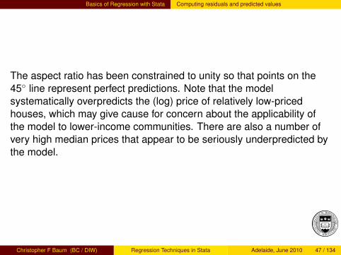
Actual vs. predicted housing prices:

8.5

99.

510

10.5

11P

redi

cted

log

med

ian

hous

ing

pric

e

8 .5 9 9 .5 10 10.5 11Actual log median housing price



The aspect ratio has been constrained to unity so that points on the45 line represent perfect predictions. Note that the modelsystematically overpredicts the (log) price of relatively low-pricedhouses, which may give cause for concern about the applicability ofthe model to lower-income communities. There are also a number ofvery high median prices that appear to be seriously underpredicted bythe model.


Basics of Regression with Stata Regression with non-i.i.d. errors

Regression with non-i.i.d. errors

If the regression errors are independently and identically distributed(i .i .d .), OLS produces consistent estimates; their sampling distributionin large samples is normal with a mean at the true coefficient valuesand their VCE is consistently estimated by the standard formula.

If the zero conditional mean assumption holds but the errors are noti .i .d ., OLS produces consistent estimates whose sampling distributionin large samples is still normal with a mean at the true coefficientvalues, but whose variance cannot be consistently estimated by thestandard formula.


Basics of Regression with Stata Regression with non-i.i.d. errors

We have two options when the errors are not i .i .d . First, we can usethe consistent OLS point estimates with a different estimator of theVCE that accounts for non-i .i .d . errors. Alternatively, if we can specifyhow the errors deviate from i .i .d . in our regression model, we can usea different estimator that produces consistent and more efficient pointestimates.

The tradeoff between these two methods is that of robustness versusefficiency. In a robust approach we place fewer restrictions on theestimator: the idea being that the consistent point estimates are goodenough, although we must correct our estimator of their VCE toaccount for non-i .i .d . errors. In the efficient approach we incorporatean explicit specification of the non-i .i .d . distribution into the model. Ifthis specification is appropriate, the additional restrictions which itimplies will produce a more efficient estimator than that of the robustapproach.


Basics of Regression with Stata Robust standard errors

Robust standard errors

We will only discuss the robust approach. If the errors are conditionallyheteroskedastic and we want to apply the robust approach, we use theHuber–White–sandwich estimator of the variance of the linearregression estimator, available in most Stata estimation commands asthe robust option.



If the assumption of homoskedasticity is valid, the non-robust standarderrors are more efficient than the robust standard errors. If we areworking with a sample of modest size and the assumption ofhomoskedasticity is tenable, we should rely on non-robust standarderrors. But since robust standard errors are very easily calculated inStata, it is simple to estimate both sets of standard errors for aparticular equation and consider whether inference based on thenon-robust standard errors is fragile. In large data sets, it has becomeincreasingly common practice to report robust (orHuber–White–sandwich) standard errors.



To illustrate the use of the robust estimator of the VCE , we use adataset (fertil2) that contains data on 4,361 women from adeveloping country. The average woman in the sample is 30 years old,first bore a child at 19 and has had 3.2 children, with just under threechildren in the household. We expect that the number of children everborn is increasing in the mother’s age and decreasing in their age atfirst birth, since the latter measure indicates when they beganchildbearing. The use of contraceptives is expected to decrease thenumber of children ever born.

We want to model the number of children ever born (ceb) to eachwoman based on their age, their age at first birth (agefbrth) and anindicator of whether they regularly use a method of contraception(usemeth).



For later use we employ estimates store to preserve the results ofthis (non-displayed) regression. We then estimate the same modelusing robust standard errors (the robust option on regress), savingthose results with estimates store. The estimates tablecommand is then used to display the two sets of coefficient estimates,standard errors and t-statistics of the regression model of ceb.



. qui regress ceb age agefbrth usemeth, robust

. estimates store Robust

. estimates table nonRobust Robust, b(%9.4f) se(%5.3f) t(%5.2f) ///> title(Estimates of CEB with OLS and Robust standard errors)

Estimates of CEB with OLS and Robust standard errors

Variable nonRobust Robust

age 0.2237 0.22370.003 0.00564.89 47.99

agefbrth -0.2607 -0.26070.009 0.010-29.64 -27.26

usemeth 0.1874 0.18740.055 0.0613.38 3.09

_cons 1.3581 1.35810.174 0.1687.82 8.11

legend: b/se/t



Our priors are borne out by the estimates, although the effect ofcontraceptive use appears to be marginally significant. The robustestimates of the standard errors are quite similar to the non-robustestimates, suggesting that heteroskedasticity may not be a problem inthis sample. Naturally, we might want to conduct a formal test ofhomoskedasticity.


Basics of Regression with Stata The Newey–West estimator of the VCE

The Newey–West estimator of the VCE

In an extension to Huber–White–sandwich robust standard errors, wemay employ the Newey–West estimator that is appropriate in thepresence of arbitrary heteroskedasticity and autocorrelation, thusknown as the HAC estimator. Its use requires us to specify anadditional parameter: the maximum order of any significantautocorrelation in the disturbance process, or the maximum lag L. Onerule of thumb that has been used is to choose L =

4√

N. This estimatoris available as the Stata command newey, which may be used as analternative to regress for estimation of a regression with HACstandard errors.

Like the robust option, application of the HAC estimator does notmodify the point estimates; it only affects the VCE . Test statisticsbased on the HAC VCE are robust to arbitrary heteroskedasticityand autocorrelation as well.


Basics of Regression with Stata Testing for heteroskedasticity

Testing for heteroskedasticity

After estimating a regression model we may base a test forheteroskedasticity on the regression residuals. If the assumption ofhomoskedasticity conditional on the regressors holds, it can beexpressed as:

H0 : Var (u|X2,X3, ...,Xk ) = σ2u (21)

A test of this null hypothesis can evaluate whether the variance of theerror process appears to be independent of the explanatory variables.We cannot observe the variances of each element of the disturbanceprocess from samples of size one, but we can rely on the squaredresidual, e2

i , to be a consistent estimator of σ2i . The logic behind any

such test is that although the squared residuals will differ in magnitudeacross the sample, they should not be systematically related toanything, and a regression of squared residuals on any candidateZi should have no meaningful explanatory power.



One of the most common tests for heteroskedasticity is derived fromthis line of reasoning: the Breusch–Pagan test. The BP test, aLagrange Multiplier (LM) test, involves regressing the squares of theregression residuals on a set of variables in an auxiliary regression

e2i = d1 + d2Zi2 + d3Zi3 + ...d`Zi` + vi (22)

The Breusch–Pagan (Cook–Weisberg) test may be executed withestat hettestafter regress. If no regressor list (of Zs) isprovided, hettest employs the fitted values from the previousregression (the yi values). As mentioned above, the variables specifiedin the set of Zs could be chosen as measures which did not appear inthe original regressor list.



We consider the potential scale-related heteroskedasticity in a modelof median housing prices where the scale can be thought of as theaverage size of houses in each community, roughly measured by itsnumber of rooms.

After estimating the model, we calculate three test statistics: thatcomputed by estat hettest without arguments, which is theBreusch–Pagan test based on fitted values; estat hettest with avariable list, which uses those variables in the auxiliary regression; andWhite’s general test statistic from whitetst.



. qui regress lprice rooms crime ldist

. hettest

Breusch-Pagan / Cook-Weisberg test for heteroskedasticityHo: Constant varianceVariables: fitted values of lprice

chi2(1) = 140.84Prob > chi2 = 0.0000

. hettest rooms crime ldist

Breusch-Pagan / Cook-Weisberg test for heteroskedasticityHo: Constant varianceVariables: rooms crime ldist

chi2(3) = 252.60Prob > chi2 = 0.0000

. whitetst

White´s general test statistic : 144.0052 Chi-sq( 9) P-value = 1.5e-26

Each of these tests indicates that there is a significant degree ofheteroskedasticity related to scale in this model.


Basics of Regression with Stata Testing for serial correlation in the error distribution

Testing for serial correlation in the errordistribution

How might we test for the presence of serially correlated errors? Justas in the case of pure heteroskedasticity, we base tests of serialcorrelation on the regression residuals. In the simplest case,autocorrelated errors follow the so-called AR(1) model: anautoregressive process of order one, also known as a first-orderMarkov process:

ut = ρut−1 + vt , |ρ| < 1 (23)

where the vt are uncorrelated random variables with mean zero andconstant variance.



If we suspect that there might be autocorrelation in the disturbanceprocess of our regression model, we could use the estimated residualsto diagnose it. The empirical counterpart to ut in Equation (23) will bethe et series produced by predict. We estimate the auxiliaryregression of et on et−1 without a constant term, as the residuals havemean zero.

The resulting slope estimate is a consistent estimator of the first-orderautocorrelation coefficient ρ of the u process from Equation (23).Under the null hypothesis, ρ = 0, so that a rejection of this nullhypothesis by this Lagrange Multiplier (LM) test indicates that thedisturbance process exhibits AR(1) behavior.



A generalization of this procedure which supports testing forhigher-order autoregressive disturbances is the Lagrange Multiplier(LM) test of Breusch and Leslie Godfrey. In this test, the regressionresiduals are regressed on the original X matrix augmented with plagged residual series. The null hypothesis is that the errors areserially independent up to order p.

We illustrate the diagnosis of autocorrelation using a time seriesdataset ukrates of monthly short-term and long-term interest rateson UK government securities (Treasury bills and gilts),1952m3–1995m12.



The model expresses the monthly change in the short rate rs, theBank of England’s monetary policy instrument as a function of the priormonth’s change in the long-term rate r20. The regressor andregressand are created on the fly by Stata’s time series operators D.and L. The model represents a monetary policy reaction function.. regress D.rs LD.r20




D.rs Coef. Std. Err. t P>|t| [95% Conf. Interval]

r20LD. .4882883 .0671484 7.27 0.000 .356374 .6202027

_cons .0040183 .022384 0.18 0.858 -.0399555 .0479921

. predict double eps, residual(2 missing values generated)



The Breusch–Godfrey test performed here considers the null of serialindependence up to sixth order in the disturbance process, and thatnull is soundly rejected. We also present an unconditional test—theLjung–Box Q test, available as command wntestq.. estat bgodfrey, lags(6)

Breusch-Godfrey LM test for autocorrelation

lags(p) chi2 df Prob > chi2

6 17.237 6 0.0084

H0: no serial correlation

. wntestq eps

Portmanteau test for white noise

Portmanteau (Q) statistic = 82.3882Prob > chi2(40) = 0.0001

Both tests decisively reject the null of no serial correlation.


Basics of Regression with Stata Regression with indicator variables

Regression with indicator variables

Economic and financial data come in three flavors: quantitative (orcardinal), ordinal (or ordered) and qualitative. Regression analysishandles quantitative data where both regressor and regressand maytake on any real value. We also may work with ordinal or ordered data.They are distinguished from cardinal measurements in that an ordinalmeasure can only express inequality of two items, and not themagnitude of their difference.

We frequently encounter data that are purely qualitative, lacking anyobvious ordering. If these data are coded as string variables, such asM and F for survey respondents’ genders, we are not likely to mistakethem for quantitative values. But in other cases, where a quality maybe coded numerically, there is the potential to misuse thisqualitative factor as quantitative.


Basics of Regression with Stata One-way ANOVA

One-way ANOVA

In order to test the hypothesis that a qualitative factor has an effect ona response variable, we must convert the qualitative factor into a set ofindicator variables, or dummy variables. We then conduct a joint teston their coefficients. If the hypothesis to be tested includes a singlequalitative factor, the estimation problem may be described as aone-way analysis of variance, or one-way ANOVA. ANOVA modelsmay be expressed as linear regressions on an appropriate set ofindicator variables.


Basics of Regression with Stata One-way ANOVA

This notion of the equivalence of one-way ANOVA and linearregression on a set of indicator variables that correspond to a singlequalitative factor generalizes to multiple qualitative factors.

If there are two qualitative factors (e.g., race and sex) that arehypothesized to affect income, a researcher would regress income ontwo appropriate sets of indicator variables, each representing one ofthe qualitative factors. This is then an example of two-way ANOVA.


Basics of Regression with Stata Using factor variables

Using factor variables

One of the biggest innovations in Stata version 11 is the introduction offactor variables. Just as Stata’s time series operators allow you to referto lagged variables (L. or differenced variables (D.), the i. operatorallows you to specify factor variables for any non-negativeinteger-valued variable in your dataset.

In the auto.dta dataset, where rep78 takes on values 1. . . 5, youcould list rep78 i.rep78, or summarize i.rep78, orregress mpg i.rep78. Each one of those commands produces theappropriate indicator variables ‘on-the-fly’: not as permanent variablesin your dataset, but available for the command.


Basics of Regression with Stata Using factor variables

For the list command, the variables will be named 1b.rep78,2.rep78 ...5.rep78. The b. is the base level indicator, by defaultassigned to the smallest value. You can specify other base levels, suchas the largest value, the most frequent value, or a particular value.

For the summarize command, only levels 2. . . 5 will be shown; thebase level is excluded from the list. Likewise, in a regression oni.rep78, the base level is the variable excluded from the regressorlist to prevent perfect collinearity. The conditional mean of the excludedvariable appears in the constant term.


Basics of Regression with Stata Interaction effects

Interaction effects

If this was the only feature of factor variables (being instantiated whencalled for) they would not be very useful. The real advantage of thesevariables is the ability to define interaction effects for bothinteger-valued and continuous variables. For instance, consider theindicator foreign in the auto dataset. We may use a new operator,#, to define an interaction:

regress mpg i.rep78 i.foreign i.rep78#i.foreign

All combinations of the two categorical variables will be defined, andincluded in the regression as appropriate (omitting base levels andcells with no observations).



In fact, we can specify this model more simply: rather than

regress mpg i.rep78 i.foreign i.rep78#i.foreign

we can use the factorial interaction operator, ##:

regress mpg i.rep78##i.foreign

which will provide exactly the same regression, producing all first-leveland second-level interactions. Interactions are not limited to pairs ofvariables; up to eight factor variables may be included.



Furthermore, factor variables may be interacted with continuousvariables to produce analysis of covariance models. The continuousvariables are signalled by the new c. operator:

regress mpg i.foreign i.foreign#c.displacement

which essentially estimates two regression lines: one for domesticcars, one for foreign cars. Again, the factorial operator could be usedto estimate the same model:

regress mpg i.foreign##c.displacement



As we will see in discussing marginal effects, it is very advantageousto use this syntax to describe interactions, both among categoricalvariables and between categorical variables and continuous variables.Indeed, it is likewise useful to use the same syntax to describesquared (and cubed. . . ) terms:

regress mpg i.foreign c.displacement c.displacement#c.displacement

In this model, we allow for an intercept shift for foreign, but constrainthe slopes to be equal across foreign and domestic cars. However, byusing this syntax, we may ask Stata to calculate the marginal effect∂mpg/∂displacement , taking account of the squared term as well, asStata understands the mathematics of the specification in this explicitform.


Basics of Regression with Stata Computing marginal effects

Computing marginal effects

With the introduction of factor variables in Stata 11, a powerful newcommand has been added: margins, which supersedes earlierversions’ mfx and adjust commands. Those commands remainavailable, but the new command has many advantages. Like thosecommands, margins is used after an estimation command.

In the simplest case, margins applied after a simple one-way ANOVAestimated with regress i.rep78, with margins i.rep78, merelydisplays the conditional means for each category of rep78.



. regress mpg i.rep78


Model 549.415777 4 137.353944 Prob > F = 0.0016Residual 1790.78712 64 27.9810488 R-squared = 0.2348

Adj R-squared = 0.1869Total 2340.2029 68 34.4147485 Root MSE = 5.2897

mpg Coef. Std. Err. t P>|t| [95% Conf. Interval]

rep782 -1.875 4.181884 -0.45 0.655 -10.22927 6.4792743 -1.566667 3.863059 -0.41 0.686 -9.284014 6.1506814 .6666667 3.942718 0.17 0.866 -7.209818 8.5431525 6.363636 4.066234 1.56 0.123 -1.759599 14.48687

_cons 21 3.740391 5.61 0.000 13.52771 28.47229



. margins i.rep78

Adjusted predictions Number of obs = 69Model VCE : OLS

Expression : Linear prediction, predict()

Delta-methodMargin Std. Err. z P>|z| [95% Conf. Interval]

rep781 21 3.740391 5.61 0.000 13.66897 28.331032 19.125 1.870195 10.23 0.000 15.45948 22.790523 19.43333 .9657648 20.12 0.000 17.54047 21.32624 21.66667 1.246797 17.38 0.000 19.22299 24.110345 27.36364 1.594908 17.16 0.000 24.23767 30.4896



We now estimate a model including both displacement and its square:. regress mpg i.foreign c.displacement c.displacement#c.displacement


Model 1416.01205 3 472.004018 Prob > F = 0.0000Residual 1027.44741 70 14.6778201 R-squared = 0.5795

Adj R-squared = 0.5615Total 2443.45946 73 33.4720474 Root MSE = 3.8312

mpg Coef. Std. Err. t P>|t| [95% Conf. Interval]

1.foreign -2.88953 1.361911 -2.12 0.037 -5.605776 -.1732833displacement -.1482539 .0286111 -5.18 0.000 -.2053169 -.0911908

c.displacement#

c.displacement .0002116 .0000583 3.63 0.001 .0000953 .0003279

_cons 41.40935 3.307231 12.52 0.000 34.81328 48.00541



margins can then properly evaluate the regression function fordomestic and foreign cars at selected levels of displacement:. margins i.foreign, at(displacement=(100 300))

Adjusted predictions Number of obs = 74Model VCE : OLS

Expression : Linear prediction, predict()

1._at : displacement = 100


Delta-methodMargin Std. Err. z P>|z| [95% Conf. Interval]

_at#foreign1 0 28.69991 1.216418 23.59 0.000 26.31578 31.084051 1 25.81038 .8317634 31.03 0.000 24.18016 27.440612 0 15.97674 .7014015 22.78 0.000 14.60201 17.351462 1 13.08721 1.624284 8.06 0.000 9.903668 16.27074



In earlier versions of Stata, calculation of marginal effects in this modelrequired some programming due to the nonlinear termdisplacement. Using margins, dydx, that is now simple.Furthermore, and most importantly, the default behavior of margins isto calculate average marginal effects (AMEs) rather than marginaleffects at the average (MAE) or at some other point in the space of theregressors. In Stata 10, the user-written command margeff (TamasBartus, on the SSC Archive) was required to compute AMEs.

Current practice favors the use of AMEs: the computation of eachobservation’s marginal effect with respect to an explanatory factor,averaged over the estimation sample, to the computation of MAEs(which reflect an average individual: e.g. a family with 2.3 children).



We illustrate by computing average marginal effects (AMEs) for theprior regression:. margins, dydx(foreign displacement)

Average marginal effects Number of obs = 74Model VCE : OLS

Expression : Linear prediction, predict()dy/dx w.r.t. : 1.foreign displacement

Delta-methoddy/dx Std. Err. z P>|z| [95% Conf. Interval]

1.foreign -2.88953 1.361911 -2.12 0.034 -5.558827 -.2202327displacement -.0647596 .007902 -8.20 0.000 -.0802473 -.049272

Note: dy/dx for factor levels is the discrete change from the base level.



Alternatively, we may compute elasticities or semi-elasticities:. margins, eyex(displacement) at(displacement=(100(100)400))


Expression : Linear prediction, predict()ey/ex w.r.t. : displacement





Delta-methodey/ex Std. Err. z P>|z| [95% Conf. Interval]

displacement_at1 -.3813974 .0537804 -7.09 0.000 -.486805 -.27598982 -.6603459 .0952119 -6.94 0.000 -.8469578 -.4737343 -.4261477 .193751 -2.20 0.028 -.8058926 -.04640284 .5613844 .4817784 1.17 0.244 -.3828839 1.505653



Consider a model where we specify a factorial interaction betweencategorical and continuous covariates:

regress mpg i.foreign i.rep78##c.displacement

In this specification, each level of rep78 has its own intercept andslope, whereas foreign only shifts the intercept term.

We may compute elasticities or semi-elasticities with the over optionof margins for all combinations of foreign and rep78:



. margins, eyex(displacement) over(foreign rep78)


Expression : Linear prediction, predict()ey/ex w.r.t. : displacementover : foreign rep78

Delta-methodey/ex Std. Err. z P>|z| [95% Conf. Interval]

displacementforeign#rep780 1 -.7171875 .5342 -1.34 0.179 -1.7642 .32982530 2 -.5953046 .219885 -2.71 0.007 -1.026271 -.16433790 3 -.4620597 .0999242 -4.62 0.000 -.6579077 -.26621180 4 -.6327362 .1647866 -3.84 0.000 -.955712 -.30976040 5 -.8726071 .0983042 -8.88 0.000 -1.06528 -.67993451 3 -.128192 .0228214 -5.62 0.000 -.1729213 -.08346281 4 -.1851193 .0380458 -4.87 0.000 -.2596876 -.1105511 5 -1.689962 .3125979 -5.41 0.000 -2.302642 -1.077281



The margins command has many other capabilities which we will notdiscuss here. Perusal of the reference manual article on marginswould be useful to explore its additional features.


Instrumental variables estimators

Regression with instrumental Variables

What are instrumental variables (IV) methods? Most widely known asa solution to endogenous regressors: explanatory variables correlatedwith the regression error term, IV methods provide a way tononetheless obtain consistent parameter estimates.

Although IV estimators address issues of endogeneity, the violation ofthe zero conditional mean assumption caused by endogenousregressors can also arise for two other common causes: measurementerror in regressors (errors-in-variables) and omitted-variable bias. Thelatter may arise in situations where a variable known to be relevant forthe data generating process is not measurable, and no good proxiescan be found.



First let us consider a path diagram illustrating the problem addressedby IV methods. We can use ordinary least squares (OLS) regression toconsistently estimate a model of the following sort.

Standard regression: y = xb + uno association between x and u; OLS consistent

x - y

u*



However, OLS regression breaks down in the following circumstance:

Endogeneity: y = xb + ucorrelation between x and u; OLS inconsistent

x - y

u

*

6

The correlation between x and u (or the failure of the zero conditionalmean assumption E [u|x ] = 0) can be caused by any of several factors.


Instrumental variables estimators Endogeneity

Endogeneity

We have stated the problem as that of endogeneity: the notion that twoor more variables are jointly determined in the behavioral model. Thisarises naturally in the context of a simultaneous equations model suchas a supply-demand system in economics, in which price and quantityare jointly determined in the market for that good or service.

A shock or disturbance to either supply or demand will affect both theequilibrium price and quantity in the market, so that by constructionboth variables are correlated with any shock to the system. OLSmethods will yield inconsistent estimates of any regression includingboth price and quantity, however specified.



As a different example, consider a cross-sectional regression of publichealth outcomes (say, the proportion of the population in various citiessuffering from a particular childhood disease) on public healthexpenditures per capita in each of those cities. We would hope to findthat spending is effective in reducing incidence of the disease, but wealso must consider the reverse causality in this relationship, where thelevel of expenditure is likely to be partially determined by the historicalincidence of the disease in each jurisdiction.

In this context, OLS estimates of the relationship will be biased even ifadditional controls are added to the specification. Although we mayhave no interest in modeling public health expenditures, we must beable to specify such an equation in order to identify the relationship ofinterest, as we discuss henceforth.



The solution provided by IV methods may be viewed as:

Instrumental variables regression: y = xb + uz uncorrelated with u, correlated with x

z - x - y

u

*6

The additional variable z is termed an instrument for x . In general, wemay have many variables in x , and more than one x correlated with u.In that case, we shall need at least that many variables in z.


Instrumental variables estimators Choice of instruments

Choice of instruments

To deal with the problem of endogeneity in a supply-demand system, acandidate z will affect (e.g.) the quantity supplied of the good, but notdirectly impact the demand for the good. An example for an agriculturalcommodity might be temperature or rainfall: clearly exogenous to themarket, but likely to be important in the production process.

For the public health example, we might use per capita income in eachcity as an instrument or z variable. It is likely to influence public healthexpenditure, as cities with a larger tax base might be expected tospend more on all services, and will not be directly affected by theunobserved factors in the primary relationship.


Instrumental variables estimators Choice of instruments

But why should we not always use IV?

It may be difficult to find variables that can serve as valid instruments.Many variables that have an effect on included endogenous variablesalso have a direct effect on the dependent variable.

IV estimators are innately biased, and their finite-sample propertiesare often problematic. Thus, most of the justification for the use of IV isasymptotic. Performance in small samples may be poor.

The precision of IV estimates is lower than that of OLS estimates (leastsquares is just that). In the presence of weak instruments (excludedinstruments only weakly correlated with included endogenousregressors) the loss of precision will be severe, and IV estimates maybe no improvement over OLS. This suggests we need a method todetermine whether a particular regressor must be treated asendogenous.


The IV-GMM estimator

IV estimation as a GMM problem

Before discussing further the motivation for various weak instrumentdiagnostics, we define the setting for IV estimation as a GeneralizedMethod of Moments (GMM) optimization problem. Economistsconsider GMM to be the invention of Lars Hansen in his 1982Econometrica paper, but as Alistair Hall points out in his 2005 book,the method has its antecedents in Karl Pearson’s Method of Moments[MM] (1895) and Neyman and Egon Pearson’s minimum Chi-squaredestimator [MCE] (1928). Their MCE approach overcomes the difficultywith MM estimators when there are more moment conditions thanparameters to be estimated. This was recognized by Ferguson (Ann.Math. Stat. 1958) for the case of i .i .d . errors, but his work had noimpact on the econometric literature.


The IV-GMM estimator

We consider the model

y = Xβ + u, u ∼ (0,Ω)

with X (N × k) and define a matrix Z (N × `) where ` ≥ k . This is theGeneralized Method of Moments IV (IV-GMM) estimator. The `instruments give rise to a set of ` moments:

gi(β) = Z ′i ui = Z ′i (yi − xiβ), i = 1,N

where each gi is an `-vector. The method of moments approachconsiders each of the ` moment equations as a sample moment, whichwe may estimate by averaging over N:

g(β) =1N

N∑i=1

zi(yi − xiβ) =1N

Z ′u

The GMM approach chooses an estimate that solves g(βGMM) = 0.


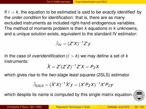
The IV-GMM estimator Exact identification and 2SLS

If ` = k , the equation to be estimated is said to be exactly identified bythe order condition for identification: that is, there are as manyexcluded instruments as included right-hand endogenous variables.The method of moments problem is then k equations in k unknowns,and a unique solution exists, equivalent to the standard IV estimator:

βIV = (Z ′X )−1Z ′y

In the case of overidentification (` > k ) we may define a set of kinstruments:

X = Z ′(Z ′Z )−1Z ′X = PZ X

which gives rise to the two-stage least squares (2SLS) estimator

β2SLS = (X ′X )−1X ′y = (X ′PZ X )−1X ′PZ y

which despite its name is computed by this single matrix equation.


The IV-GMM estimator The IV-GMM approach

The IV-GMM approach

In the 2SLS method with overidentification, the ` available instrumentsare “boiled down" to the k needed by defining the PZ matrix. In theIV-GMM approach, that reduction is not necessary. All ` instrumentsare used in the estimator. Furthermore, a weighting matrix is employedso that we may choose βGMM so that the elements of g(βGMM) are asclose to zero as possible. With ` > k , not all ` moment conditions canbe exactly satisfied, so a criterion function that weights themappropriately is used to improve the efficiency of the estimator.

The GMM estimator minimizes the criterion

J(βGMM) = N g(βGMM)′W g(βGMM)

where W is a `× ` symmetric weighting matrix.


The IV-GMM estimator The GMM weighting matrix

Solving the set of FOCs, we derive the IV-GMM estimator of anoveridentified equation:

βGMM = (X ′ZWZ ′X )−1X ′ZWZ ′y

which will be identical for all W matrices which differ by a factor ofproportionality. The optimal weighting matrix, as shown by Hansen(1982), chooses W = S−1 where S is the covariance matrix of themoment conditions to produce the most efficient estimator:

S = E [Z ′uu′Z ] = limN→∞ N−1[Z ′ΩZ ]

With a consistent estimator of S derived from 2SLS residuals, wedefine the feasible IV-GMM estimator as

βFEGMM = (X ′Z S−1Z ′X )−1X ′Z S−1Z ′y

where FEGMM refers to the feasible efficient GMM estimator.


The IV-GMM estimator IV-GMM and the distribution of u

The derivation makes no mention of the form of Ω, thevariance-covariance matrix (vce) of the error process u. If the errorssatisfy all classical assumptions are i .i .d ., S = σ2

uIN and the optimalweighting matrix is proportional to the identity matrix. The IV-GMMestimator is merely the standard IV (or 2SLS) estimator.

If there is heteroskedasticity of unknown form, we usually computerobust standard errors in any Stata estimation command to derive aconsistent estimate of the vce. In this context,

S =1N

N∑i=1

u2i Z ′i Zi

where u is the vector of residuals from any consistent estimator of β(e.g., the 2SLS residuals). For an overidentified equation, the IV-GMMestimates computed from this estimate of S will be more efficientthan 2SLS estimates.


The IV-GMM estimator IV-GMM and the distribution of u

We must distinguish the concept of IV/2SLS estimation with robuststandard errors from the concept of estimating the same equation withIV-GMM, allowing for arbitrary heteroskedasticity. Compare anoveridentified regression model estimated (a) with IV and classicalstandard errors and (b) with robust standard errors. Model (b) willproduce the same point estimates, but different standard errors in thepresence of heteroskedastic errors.

However, if we reestimate that overidentified model using the GMMtwo-step estimator, we will get different point estimates because weare solving a different optimization problem: one in the `-space of theinstruments (and moment conditions) rather than the k -space of theregressors, and ` > k . We will also get different standard errors, and ingeneral smaller standard errors as the IV-GMM estimator is moreefficient. This does not imply, however, that summary measuresof fit will improve.


The IV-GMM estimator IV-GMM cluster-robust estimates

If errors are considered to exhibit arbitrary intra-cluster correlation in adataset with M clusters, we may derive a cluster-robust IV-GMMestimator using

S =M∑

j=1

u′j uj

whereuj = (yj − xj β)X ′Z (Z ′Z )−1zj

The IV-GMM estimates employing this estimate of S will be both robustto arbitrary heteroskedasticity and intra-cluster correlation, equivalentto estimates generated by Stata’s cluster(varname) option. For anoveridentified equation, IV-GMM cluster-robust estimates will be moreefficient than 2SLS estimates.


The IV-GMM estimator IV-GMM HAC estimates

The IV-GMM approach may also be used to generate HAC standarderrors: those robust to arbitrary heteroskedasticity and autocorrelation.Although the best-known HAC approach in econometrics is that ofNewey and West, using the Bartlett kernel (per Stata’s newey), that isonly one choice of a HAC estimator that may be applied to an IV-GMMproblem. Baum–Schaffer–Stillman’s ivreg2 (from the SSC Archive)and Stata 10’s ivregress provide several choices for kernels. Forsome kernels, the kernel bandwidth (roughly, number of lagsemployed) may be chosen automatically in either command.


The IV-GMM estimator Implementation in Stata

The ivreg2 command

The estimators we have discussed are available from Baum, Schafferand Stillman’s ivreg2 package (ssc describe ivreg2). Theivreg2 command has the same basic syntax as Stata’s older ivregcommand:

ivreg2 depvar [varlist1] (varlist2=instlist) ///[if] [in] [, options]

The ` variables in varlist1 and instlist comprise Z , the matrix ofinstruments. The k variables in varlist1 and varlist2 compriseX . Both matrices by default include a units vector.


The IV-GMM estimator ivreg2 options

By default ivreg2 estimates the IV estimator, or 2SLS estimator if` > k . If the gmm2s option is specified in conjunction with robust,cluster() or bw(), it estimates the IV-GMM estimator.

With the robust option, the vce is heteroskedasticity-robust.

With the cluster(varname) option, the vce is cluster-robust.

With the robust and bw( ) options, the vce is HAC with the defaultBartlett kernel, or “Newey–West”. Other kernel( ) choices lead toalternative HAC estimators. In ivreg2, both robust and bw( )options must be specified for HAC. Estimates produced with bw( )alone are robust to arbitrary autocorrelation but assumehomoskedasticity.


The IV-GMM estimator Example of IV and IV-GMM estimation

Example of IV and IV-GMM estimation

We illustrate with a wage equation estimated from the Grilichesdataset (griliches76) of very young men’s wages. Their log(wage)is explained by completed years of schooling, experience, job tenureand IQ score.

The IQ variable is considered endogenous, and instrumented withthree factors: their mother’s level of education (med), their score on astandardized test (kww) and their age. The estimation in ivreg2 isperformed with

ivreg2 lw s expr tenure (iq = med kww age)

where the parenthesized expression defines the included endogenousand excluded exogenous variables. You could also use official Stata’sivregress 2sls.



. esttab, label stat(rmse) mtitles(IV IVrob IVGMMrob) nonum

IV IVrob IVGMMrob

iq score -0.00509 -0.00509 -0.00676(-1.06) (-1.01) (-1.34)

completed years of~g 0.122*** 0.122*** 0.128***(7.68) (7.51) (7.88)

experience, years 0.0357*** 0.0357*** 0.0368***(5.15) (5.10) (5.26)

tenure, years 0.0405*** 0.0405*** 0.0443***(4.78) (4.51) (4.96)

Constant 4.441*** 4.441*** 4.523***(14.22) (13.21) (13.46)

rmse 0.366 0.366 0.372

t statistics in parentheses

* p<0.05, ** p<0.01, *** p<0.001



These three columns compare standard IV (2SLS) estimates, IV withrobust standard errors, and IV-GMM with robust standard errors,respectively. Notice that the coefficients’ point estimates change whenIV-GMM is employed, and that their t-statistics are larger than those ofrobust IV. Note also that the IQ score is not significant in any of thesemodels.


Tests of overidentifying restrictions


If and only if an equation is overidentified, we may test whether theexcluded instruments are appropriately independent of the errorprocess. That test should always be performed when it is possible todo so, as it allows us to evaluate the validity of the instruments.

A test of overidentifying restrictions regresses the residuals from an IVor 2SLS regression on all instruments in Z . Under the null hypothesisthat all instruments are uncorrelated with u, the test has alarge-sample χ2(r) distribution where r is the number of overidentifyingrestrictions.



Under the assumption of i .i .d . errors, this is known as a Sargan test,and is routinely produced by ivreg2 for IV and 2SLS estimates. It canalso be calculated after ivreg estimation with the overid command,which is part of the ivreg2 suite. After ivregress, the commandestat overid provides the test.



If we have used IV-GMM estimation in ivreg2, the test ofoveridentifying restrictions becomes J: the GMM criterion function.Although J will be identically zero for any exactly-identified equation, itwill be positive for an overidentified equation. If it is “too large”, doubt iscast on the satisfaction of the moment conditions underlying GMM.

The test in this context is known as the Hansen test or J test, and iscalculated by ivreg2 when the gmm2s option is employed.

The Sargan–Hansen test of overidentifying restrictions should beperformed routinely in any overidentified model estimated withinstrumental variables techniques. Instrumental variables techniquesare powerful, but if a strong rejection of the null hypothesis of theSargan–Hansen test is encountered, you should strongly doubt thevalidity of the estimates.



For instance, let’s rerun the last IV-GMM model we estimated andfocus on the test of overidentifying restrictions provided by the HansenJ statistic. The model is overidentified by two degrees of freedom, asthere is one endogenous regressor and three excluded instruments.We see that the J statistic strongly rejects its null, casting doubts onthe quality of these estimates.

Let’s reestimate the model excluding age from the instrument list andsee what happens. We will see that the sign and significance of the keyendogenous regressor changes as we respecify the instrument list,and the p-value of the J statistic becomes large when age is excluded.



Example: Test of overidentifying restrictions

. esttab, label stat(j jdf jp) mtitles(age no_age) nonum

age no_age

iq score -0.00676 0.0181**(-1.34) (2.97)

completed years of~g 0.128*** 0.0514**(7.88) (2.63)

experience, years 0.0368*** 0.0440***(5.26) (5.58)

tenure, years 0.0443*** 0.0303***(4.96) (3.48)

Constant 4.523*** 2.989***(13.46) (7.58)

j 49.84 0.282jdf 2 1jp 1.50e-11 0.595

t statistics in parentheses

* p<0.05, ** p<0.01, *** p<0.001

. sjlog close


Tests of overidentifying restrictions Testing a subset of overidentifying restrictions

We may be quite confident of some instruments’ independence from ubut concerned about others. In that case a GMM distance or C testmay be used. The orthog( ) option of ivreg2 tests whether asubset of the model’s overidentifying restrictions appear to be satisfied.

This is carried out by calculating two Sargan–Hansen statistics: one forthe full model and a second for the model in which the listed variablesare (a) considered endogenous, if included regressors, or (b) dropped,if excluded regressors. In case (a), the model must still satisfy theorder condition for identification. The difference of the twoSargan–Hansen statistics, often termed the GMM distance or Cstatistic, will be distributed χ2 under the null hypothesis that thespecified orthogonality conditions are satisfied, with d.f. equal to thenumber of those conditions.



A variant on this strategy is implemented by the endog( ) option ofivreg2, in which one or more variables considered endogenous canbe tested for exogeneity. The C test in this case will consider whetherthe null hypothesis of their exogeneity is supported by the data.

If all endogenous regressors are included in the endog( ) option, thetest is essentially a test of whether IV methods are required toestimate the equation. If OLS estimates of the equation are consistent,they should be preferred. In this context, the test is equivalent to aHausman test comparing IV and OLS estimates, as implemented byStata’s hausman command with the sigmaless option. Usingivreg2, you need not estimate and store both models to generate thetest’s verdict.



For instance, with the model above, we might question whether IVtechniques are needed. We can conduct the C test via:

ivreg2 lw s expr tenure (iq=med kww), gmm2s robust endog(iq)

where the endog(iq) option tests the null hypothesis that iq isproperly exogenous in this model. The test statistic has a p-value of0.0108, suggesting that the data overwhelmingly reject the use of OLSin favor of IV. At the same time, the J statistic (with a p-value of 0.60)indicates that the overidentifying restrictions are not rejected.


Testing for weak instruments

The weak instruments problem

Instrumental variables methods rely on two assumptions: the excludedinstruments are distributed independently of the error process, andthey are sufficiently correlated with the included endogenousregressors. Tests of overidentifying restrictions address the firstassumption, although we should note that a rejection of their null maybe indicative that the exclusion restrictions for these instruments maybe inappropriate. That is, some of the instruments have beenimproperly excluded from the regression model’s specification.



The specification of an instrumental variables model asserts that theexcluded instruments affect the dependent variable only indirectly,through their correlations with the included endogenous variables. Ifan excluded instrument exerts both direct and indirect influences onthe dependent variable, the exclusion restriction should be rejected.This can be readily tested by including the variable as a regressor.

In our earlier example we saw that including age in the excludedinstruments list caused a rejection of the J test. We had assumed thatage could be treated as excluded from the model. Is that assumptionwarranted?

If age is entered as a regressor, it has a t-statistic over 8. Thus, itsrejection as an excluded instrument may well reflect themisspecification of the equation, omitting age.



To test the second assumption—that the excluded instruments aresufficiently correlated with the included endogenous regressors—weshould consider the goodness-of-fit of the “first stage” regressionsrelating each endogenous regressor to the entire set of instruments.

It is important to understand that the theory of single-equation (“limitedinformation”) IV estimation requires that all columns of X areconceptually regressed on all columns of Z in the calculation of theestimates. We cannot meaningfully speak of “this variable is aninstrument for that regressor” or somehow restrict which instrumentsenter which first-stage regressions. Stata’s ivregress or ivreg2 willnot let you do that because such restrictions only make sense in thecontext of estimating an entire system of equations by full-informationmethods (for instance, with reg3).



The first and ffirst options of ivreg2 present several usefuldiagnostics that assess the first-stage regressions. If there is a singleendogenous regressor, these issues are simplified, as the instrumentseither explain a reasonable fraction of that regressor’s variability or not.With multiple endogenous regressors, diagnostics are morecomplicated, as each instrument is being called upon to play a role ineach first-stage regression.

With sufficiently weak instruments, the asymptotic identification statusof the equation is called into question. An equation identified by theorder and rank conditions in a finite sample may still be effectivelyunidentified.



As Staiger and Stock (Econometrica, 1997) show, the weakinstruments problem can arise even when the first-stage t- and F -testsare significant at conventional levels in a large sample. In the worstcase, the bias of the IV estimator is the same as that of OLS, IVbecomes inconsistent, and instrumenting only aggravates the problem.



Beyond the informal “rule-of-thumb” diagnostics such as F > 10,ivreg2 computes several statistics that can be used to criticallyevaluate the strength of instruments. We can write the first-stageregressions as

X = Z Π + v

With X1 as the endogenous regressors, Z1 the excluded instrumentsand Z2 as the included instruments, this can be partitioned as

X1 = [Z1Z2] [Π′11Π′12]′ + v1

The rank condition for identification states that the L× K1 matrix Π11must be of full column rank.


Testing for weak instruments The Anderson canonical correlation statistic

We do not observe the true Π11, so we must replace it with anestimate. Anderson’s (John Wiley, 1984) approach to testing the rankof this matrix (or that of the full Π matrix) considers the canonicalcorrelations of the X and Z matrices. If the equation is to be identified,all K of the canonical correlations will be significantly different fromzero.

The squared canonical correlations can be expressed as eigenvaluesof a matrix. Anderson’s CC test considers the null hypothesis that theminimum canonical correlation is zero. Under the null, the test statisticis distributed χ2 with (L− K + 1) d.f., so it may be calculated even foran exactly-identified equation. Failure to reject the null suggests theequation is unidentified. ivreg2 reports this Lagrange Multiplier (LM)statistic.


Testing for weak instruments The Cragg–Donald statistic

The Cragg–Donald statistic is a closely related test of the rank of amatrix. While the Anderson CC test is a LR test, the C–D test is aWald statistic, with the same asymptotic distribution. The C–D statisticplays an important role in Stock and Yogo’s work (see below). Both theAnderson and C–D tests are reported by ivreg2 with the firstoption.

Recent research by Kleibergen and Paap (KP) (J. Econometrics, 2006)has developed a robust version of a test for the rank of a matrix: e.g.testing for underidentification. The statistic has been implemented byKleibergen and Schaffer as command ranktest. If non-i .i .d . errorsare assumed, the ivreg2 output contains the K–P rk statistic in placeof the Anderson canonical correlation statistic as a test ofunderidentification.


Testing for weak instruments The Stock and Yogo approach

Stock and Yogo (Camb. U. Press festschrift, 2005) propose testing forweak instruments by using the F -statistic form of the C–D statistic.Their null hypothesis is that the estimator is weakly identified in thesense that it is subject to bias that the investigator finds unacceptablylarge.

Their test comes in two flavors: maximal relative bias (relative to thebias of OLS) and maximal size. The former test has the null thatinstruments are weak, where weak instruments are those that can leadto an asymptotic relative bias greater than some level b. This test usesthe finite sample distribution of the IV estimator, and can only becalculated where the appropriate moments exist (when the equation issuitably overidentified: the mth moment exists iff m < (L−K + 1)). Thetest is routinely reported in ivreg2 and ivregress output when itcan be calculated, with the relevant critical values calculated byStock and Yogo.


Testing for weak instruments The Stock and Yogo approach

The second test proposed by Stock and Yogo is based on theperformance of the Wald test statistic for the endogenous regressors.Under weak identification, the test rejects too often. The test statistic isbased on the rejection rate r tolerable to the researcher if the truerejection rate is 5%. Their tabulated values consider various values forr . To be able to reject the null that the size of the test is unacceptablylarge (versus 5%), the Cragg–Donald F statistic must exceed thetabulated critical value.

The Stock–Yogo test statistics, like others discussed above, assumei .i .d . errors. The Cragg–Donald F can be robustified in the absence ofi .i .d . errors by using the Kleibergen–Paap rk statistic, which ivreg2reports in that circumstance.


When you may (and may not!) use IV

When you may (and may not!) use IV

A common inquiry on Statalist: what should I do if I have anendogenous regressor that is a dummy variable? Should I, forinstance, fit a probit model to generate the “hat values”, estimate themodel with OLS including those “hat values” instead of the 0/1 values,and puzzle over what to do about the standard errors?

An aside: you really do not want to do two-stage least squares “byhand”, for one of the things that you must then deal with is getting thecorrect VCE estimate. The VCE and RMSE computed by thesecond-stage regression are not correct, as they are generated fromthe “hat values”, not the original regressors. But back to our question.


When you may (and may not!) use IV Dummy variable as endogenous regressor

Should I fit a probit model to generate the “hat values”, estimate themodel with OLS including those “hat values” instead of the 0/1 values,and puzzle over what to do about the standard errors?

No, you should just estimate the model with ivreg2 or ivregress,treating the dummy endogenous regressor like any other endogenousregressor. This yields consistent point and interval estimates of itscoefficient. There are other estimators (notably in the field of selectionmodels or treatment regression) that explicitly deal with this problem,but they impose additional conditions on the problem. If you can usethose methods, fine. Otherwise, just run IV. This solution is alsoappropriate for count data.


When you may (and may not!) use IV Dummy variable as endogenous regressor

Another solution to the problem of an endogenous dummy (or countvariable), as discussed by Cameron and Trivedi, is due to Basmann(Econometrica, 1957). Obtain fitted values for the endogenousregressor with appropriate nonlinear regression (logit or probit for adummy, Poisson regression for a count variable) using all theinstruments (included and excluded). Then do regular linear IV usingthe fitted value as an instrument, but the original dummy (or countvariable) as the regressor. This is also a consistent estimator, althoughit has a different asymptotic distribution than does that of straight IV.


When you may (and may not!) use IV Equation nonlinear in endogenous variables

Equation nonlinear in endogenous variables

A second FAQ: what if my equation includes a nonlinear function of anendogenous regressor? For instance, from Wooldridge, EconometricAnalysis of Cross Section and Panel Data (2002), p. 231, we mightwrite the supply and demand equations for a good as

log qs = γ12 log(p) + γ13[log(p)]2 + δ11z1 + u1

log qd = γ22 log(p) + δ22z2 + u2

where we have suppressed intercepts for convenience. Theexogenous factor z1 shifts supply but not demand. The exogenousfactor z2 shifts demand but not supply. There are thus two exogenousvariables available for identification.



This system is still linear in parameters, and we can ignore the logtransformations on p,q. But it is, in Wooldridge’s terms, nonlinear inendogenous variables, and identification must be treated differently.



If we used these equations to obtain log(p) = y2 as a function ofexogenous variables and errors (the reduced form equation), the resultwould not be linear. E [y2|z] would not be linear unless γ13 = 0,assuming away the problem, and E [y2

2 |z] will not be linear in any case.We might imagine that y2

2 could just be treated as an additionalendogenous variable, but then we need at least one more instrument.Where do we find it?

Given the nonlinearity, other functions of z1 and z2 will appear in alinear projection with y2

2 as the dependent variable. Under linearity, thereduced form for y2 involves z1, z2 and combinations of the errors.Square that reduced form, and E [y2

2 |z] is a function of z21 , z

22 and z1z2

(and the expectation of the squared composite error). Given that thisrelation has been derived under assumptions of linearity andhomoskedasticity, we should also include the levels of z1, z2 in theprojection (first stage regression).



The supply equation may then be estimated with instrumentalvariables using z1, z2, z2

1 , z22 and z1z2 as instruments. You could also

use higher powers of the exogenous variables.

The mistake that may be made in this context involves what Hausmandubbed the forbidden regression: trying to mimic 2SLS by substitutingfitted values for some of the endogenous variables inside the nonlinearfunctions. Nether the conditional expectation of the linear projectionnor the linear projection operator passes through nonlinear functions,and such attempts “...rarely produce consistent estimators in nonlinearsystems.” (Wooldridge, p. 235)



In our example above, imagine regressing y2 on exogenous variables,saving the predicted values, and squaring them. The “second stage”regression would then regress log(q) on y , y2, z1.

This two-step procedure does not yield the same results as estimatingthe equation by 2SLS, and it generally cannot produce consistentestimates of the structural parameters. The linear projection of thesquare is not the square of the linear projection, and the “by hand”approach assumes they are identical.


Further reading

Further reading

There are many important considerations relating to the use of IVtechniques, including LIML (limited-information maximum likelihoodestimation) and GMM-CUE (continuously updated GMM estimates).For more details, please see

Enhanced routines for instrumental variables/GMM estimation andtesting. Baum CF, Schaffer ME, Stillman S, Stata Journal 7:4,2007. Boston College Economics working paper no. 667,available from http://ideas.repec.org.

An Introduction to Modern Econometrics Using Stata, Baum CF,Stata Press, 2006 (particularly Chapter 8).

Instrumental variables and GMM: Estimation and testing. BaumCF, Schaffer ME, Stillman S, Stata Journal 3:1–31, 2003.Freely available from http://stata-journal.com.


University of Adelaide, June 2010 - School of Economics · Regression Techniques in Stata...

Documents

Transcript of University of Adelaide, June 2010 - School of Economics · Regression Techniques in Stata...