1924 - DIW
37
Discussion Papers Emergency Aid for Self-Employed in the COVID-19 Pandemic: A Flash in the Pan? Joern Block, Alexander Kritikos, Maximilian Priem and Caroline Stiel 1924 Deutsches Institut für Wirtschaftsforschung 2020
Transcript of 1924 - DIW

Discussion Papers
Emergency Aid for Self-Employed in the COVID-19 Pandemic: A Flash in the Pan?
Joern Block, Alexander Kritikos, Maximilian Priem and Caroline Stiel
1924
Deutsches Institut für Wirtschaftsforschung 2020

Opinions expressed in this paper are those of the author(s) and do not necessarily reflect views of the institute.
IMPRESSUM
© DIW Berlin, 2020
DIW Berlin German Institute for Economic Research Mohrenstr. 58 10117 Berlin
Tel. +49 (30) 897 89-0 Fax +49 (30) 897 89-200 http://www.diw.de
ISSN electronic edition 1619-4535
Papers can be downloaded free of charge from the DIW Berlin website: http://www.diw.de/discussionpapers
Discussion Papers of DIW Berlin are indexed in RePEc and SSRN: http://ideas.repec.org/s/diw/diwwpp.html http://www.ssrn.com/link/DIW-Berlin-German-Inst-Econ-Res.html

1
Emergency Aid for Self-employed in the COVID-19 pandemic:A Flash in the Pan?*
Joern Block† Alexander Kritikos ‡ Maximilian Priem§ Caroline Stiel**
Trier University DIW Berlin DIW Econ DIW Berlin
December, 2020
Abstract:
The self-employed are among those facing the highest probability of strong income lossesduring the COVID-19 pandemic. Governments in many countries introduced supportprograms to support the self-employed, including the German federal government, whichapproved a €50bn emergency aid program at the end of March 2020 offering one-offlump-sum payments of up to €15,000 to those facing substantial revenue declines. In thiscontribution, we investigate the impact of this program using a real-time online-surveydata with a total of more than 20,000 observations. We employ propensity scorematching, making use of a rich set of variables that influence selection into the treatmentand the outcome variable, the subjective survival probability. We observe that theemergency aid program had significant effects, with the subjective survival probabilityof self-employment being moderately increased. We further reveal important effectheterogeneities with respect to education, risk tolerance, and industries. We also observepositive effects only among those whose application was processed within a few days.Lastly, the positive effect on the survival probability is fading out already two weeks afterthe emergency aid was granted. Our findings have important policy implications for thedesign of such support programs in the course of this crisis.
JEL Classification: C14, H43, L25, L26, J68Keywords: Self-Employment, Emergency Aid, Treatment Effects, COVID-19,Entrepreneurship
* We gratefully acknowledge the support of Thea Zöllner and the Verband der Gründer undSelbstständigen Deutschland e. V. (VGSD) who provided us with the data. Moreover, we thank DanielGraeber, Steffen Künn, and Johannes Seebauer for the valuable comments.
† Joern Block is Professor at the University of Trier, the Department of Applied Economics, ErasmusUniversity Rotterdam, and Wittener Institut für Familienunternehmen (WIFU), University ofWitten/Herdecke. e-mail: [email protected].
‡ Alexander Kritikos, (corresponding author is Research Director at the German Institute for EconomicResearch (DIW Berlin), Professor of Economics at the University of Potsdam, and Research Fellow atIZA, Bonn and at IAB, Nuremberg. Address: DIW Berlin, Mohrenstr. 58, 10117 Berlin, Germany. e-mail: [email protected]
§ Maximilian Priem is Senior Data Scientist at DIW Econ., e-mail: [email protected]** Caroline Stiel is Senior Research Associate at the German Institute for Economic Research (DIW
Berlin), e-mail: [email protected]

1
1. Introduction
The unprecedented shutdown of businesses, especially of those in the service sector and
the trade industries, as well as general insecurity, has led in many countries to a temporary
closure of major parts of their economies in spring 2020. The affected industries depend
more on the self-employed and micro businesses (collectively referred to as “self-
employed” from now on) than the manufacturing sector. First evidence points to the fact
that the self-employed population has suffered more strongly from the disruption caused
by the COVID-19 pandemic than other parts of the working population in relative terms.
In Germany, for instance, about 60% of the self-employed faced sales and income losses,
while only about 15% of dependently employed individuals confronted job or wage losses
(see Kritikos et al. 2020).1 Therefore, in addition to Kurzarbeit, Germany’s short time work
compensation scheme that is a well-established safety net for employees (see Cahuc 2014),
the German government introduced at the end of March 2020 an emergency aid program
designed to financially support those self-employed who faced strong revenue declines.
The main aim of this paper is to investigate the effects of this program on the subjective
survival probability among the supported self-employed.
In Germany, around 4.2 million individuals (about 10% of the working population)
are self-employed, either without any employees (so called solo self-employed, see e.g. de
Vries et al. 2019) and sometimes with hourly earnings around the minimum wage (Sorgner
et al. 2017) or with employees, often running micro businesses with fewer than 10
employees (hereafter “employers”). This diverse population of self-employed, which has
grown strongly since the 1990s, is an increasingly important part of the German economy,
from both labor market and economic perspectives. This role is not limited to creating their
own and other jobs. In several parts of the service sector, such ventures are the backbone
of the economy, where the largest share of individuals are employed in firms with 10 or
fewer employees (Audretsch et al. 2020). Given the relevance of the sum of all self-
employed workers (solo self-employed and employers) for the German economy and given
that a large share of them is facing strong revenue declines and income losses during the
COVID-19 pandemic, their survival and ongoing struggles in the pandemic are of high
concern for policy makers.
1 See Crossley et al. (2021) for other employment groups that were also severely affected by this crisis.

2
In response to the crisis, the German Minister of Economics Affairs announced at a
press conference on March 10, 2020, “that we will not let any firm down”2. His ministry
introduced together with the Ministry of Finance an extensive emergency aid program
(“Soforthilfe”) of up to €50 billion to support the self-employed (including micro firms
with up to 10 employees). The program took the form of a one-off lump sum grant of up
to €15,000 per self-employed, that could be paid out of this program and was accessible
between the end of March and end of May 2020. €13.7 billion of the €50 billion were spent
through this program. In this contribution, we investigate whether the program achieved to
increase the subjective probability of the affected self-employed to get through the COVID-
19 pandemic. This research question is particularly relevant given the huge amount of
taxpayer money that was made available for this program.3
For our analysis, we rely on a survey that was answered by more than 20,000 self-
employed and that took place in April and early May 2020. Besides information on crisis
related sales losses, resulting liquidity constraints, the willingness to apply for financial
support from the emergency fund as well as on information whether financial support was
actually received, the survey recorded information on most individual- and firm-related
characteristics that are known to be relevant for self-employment activities. As outcome
variable, we focus on a measure that is based on the subjective assessment of the
individuals about the probability that they have to “end their self-employment activities
due to the Corona-crisis in the following 12 months”. Prior research (Cassar 2010,
Hyytinen et al. 2014) has used such subjective survival probability measures and has shown
its correlation with objective survival measures and relevance in entrepreneurial decision-
making. Moreover, beyond the rich information on the self-employed, we make use of the
fact that the data is surveyed in real-time recording the exact days of the respondent’s
emergency aid application as well as its approval or denial.
To be able to causally analyze whether the financial support measures increased the
subjective survival probability, we rely on the conditional independence assumption (CIA).
More specifically, we compare those self-employed who already received support out of
this program (the treated group) with those who planned to apply for the program (the
untreated group), controlling for a rich set of variables that influence the application and
2 Press conference of the Minister of Economics at March 10, 2020 (see(https://www.tagesschau.de/inland/corona-wirtschaft-105.html, accessed November 27, 2020).
3 In order to classify the budget of the program of €50bn, we point to typical measures in the area of self-employment, for instance the various start-up subsidy programs in Germany that received yearly budgetsof less than €1bn (with the exception of the year 2004, when it reached €2bn). For an evaluation of thesesubsidies, see inter alia Caliendo and Kuenn (2011).

3
survival probability. This includes also information on how severely they were hit by the
crisis and for how long they had liquidity reserves to survive the crisis.
We contribute to the literature around the analysis of the COVID-19 pandemic
(Adams-Prassl et al. 2020, Block et al. 2020, Blundell and Machin 2020, Fairlie 2020,
Graeber et al. 2020) in several ways. This crisis is unique in itself and there is, so far, no
experience how public interventions that aim to deal with the economic consequences of
the crisis, may help. It might also not be possible to infer insights from analyzing public
policies that were taken in earlier crisis situations like the financial crisis from 2008, as the
causes of the financial crisis strongly differ from the current one. In that context, we provide
first empirical evidence on the subjectively perceived effectiveness of an emergency aid
program during this pandemic. Secondly, we take advantage of real-time, individual-level
data that allow us to investigate the impact of variations in the speed of processing the
applications for emergency aid. Thirdly, we analyze effect heterogeneities with respect to
various variables, such as risk tolerance or education levels. In that sense, our analysis is
of high relevance given the ongoing debate on the right design and implementation of such
policy instruments, informing about which specific target groups perceive the public
financial support positively under the given conditions. With our results, we also contribute
to the literature on small business policy (Minniti 2008, Acs et al. 2016) in times of
economic crises, as well as on the effects of entrepreneurial optimism and subjective
survival probability (Cassar 2010, Hytytinen et al. 2014).
Based on our propensity score specification, our results show that the financial
support measure had moderately positive effects as it significantly increased the subjective
probability to survive the pandemic. We also find important effect heterogeneities as
positive effects appear, in particular, for higher educated and more risk tolerant individuals.
We further find that the positive effect (a) depends on the speed of the application approval
and (b) vanishes as more time passes since the approval.
The rest of the paper is organized as follows. In Section 2, we describe the measures
taken to control the pandemic as well as further details on the emergency aid package.
Section 3 presents the data used for the empirical analysis and some summary statistics
including a description of the economic effects that were observed among the self-
employed,. Section 4 describes the estimation strategy and the propensity score matching
approach. Section 5 presents the main estimation results together with the analysis of effect
heterogeneities and some robustness checks. Section 6 concludes.

4
2. The COVID-19 Pandemic and Related Policies
2.1 The COVID-19 Pandemic in Germany and Related Policy Measures
At the time of the data collection in April and May 2020, Germany was one of the most
affected by the COVID-19 pandemic: over 130,000 people were infected with the Virus
SARS-CoV-2. The German government tried to stop the spreading of the virus through
several measures with severe impacts on the economy. Schools and daycare centers were
closed, as well as most shops, restaurants, and hotels, except for supermarkets. A curfew
was imposed, which included a ban on public gatherings of more than two people, except
for people living in the same household. People in public areas were required to keep a
minimum distance of 1.5 meters. All major and minor events, including trade fairs, sports
events, and concerts, were cancelled; travel was restricted. During that time, the Institut für
Weltwirtschaft (IfW 2020) predicted a GDP decline of up to 9% for 2020. The self-
employed were among the most affected occupational groups, especially those working in
the hotel and restaurant business, the tourism industry, the retail sector, the cultural sector,
the events sector, and other service industries that require personal contact. For them, the
policy measures to contain the epidemic meant, in fact, a temporary prohibition to work,
where they could not generate revenues to cover their operating expenses and living costs.
2.2 Government Support Programs and Emergency Aid Packages
In order to help the economy and to avoid job cuts as well as a long-lasting recession, the
German government introduced several supporting programs to mitigate the consequences
of the pandemic. Targeting established firms, employers (including the self-employed
employers) could send their employees into Kurzarbeit, short-time work, where the Federal
Employment Office covers a substantial portion of the wage costs. This instrument allowed
employers to keep their workforce through the crisis while simultaneously protecting
employees from losing their jobs and from major wage cuts. However, the self-employed
themselves are not covered by this labor market instrument. To address this segment, the
government launched an emergency aid package (“Soforthilfe”) of €50 billion, accessible
from March 25, 2020 through the end of May 2020. The self-employed were able to apply
for this program a couple of days ahead of the official start. The goal of this package was
to help solo self-employed and owners of micro firms (with up to 10 employees), who
combined account for up about 4.2 million individuals, maintain their ventures and increase
their chances of entrepreneurial survival. This group of self-employed individuals could

5
receive immediate financial assistance of up to €15,000 - the maximum amount depended
on the number of employees in their businesses, if they were able to demonstrate acute
liquidity shortfalls (Federal Ministry for Economic Affairs and Energy, 2020). As a
downside of the instrument, the funds from the support program could only be used to
cover operating costs; private living costs were excluded.
2.3 Prior Research on Self-employment During the COVID-19 Pandemic
The effects of the COVID-19 pandemic on self-employment is attracting empirical
research. This research documents that, during the crisis, self-employed workers in other
countries suffered in similar ways to those in Germany (Adams-Prassl et al. 2020, Bartik
et al. 2020, Graeber et al. 2020). For the U.K., Blundell and Machin (2020) show that three
out of four self-employed individuals report a reduced work load. Further, the number of
active business owners declined by about 22% in the US, the largest drop ever recorded
(Fairlie 2020). Kalenkoski and Pabilonia (2020), who focus on unincorporated self-
employed workers, reveal that they were about 57 percentage points less likely to be self-
employed in April 2020 relative to February. In Canada, self-employment also fell very
strongly: Beland et al. (2020) report an activity decline of 14.8% for incorporated and
10.1% for unincorporated entities. These examples show that the decline of self-
employment in response to the pandemic is a global phenomenon. Block et al. (2020)
investigate how the self-employed cope with the COVID-19 pandemic and maintain their
liquidity, particularly through the use of bootstrap financing. They find that this financing
instrument is used by many self-employed, and is, amongst others, positively associated
with the severity of the crisis for the venture, the level of private consumption, and self-
employment experience. Finally, using German data, Bertschek and Erdsiek (2020) show
that self-employed with a higher degree of digitization are less affected by the crisis.
3 Data
3.1 Data Description of the Estimation Sample
Our survey took place between April 7 and May 4, 2020. Data was collected via an online
survey. The survey, collecting information with respect to the pandemic for the self-
employed, covered the characteristics of the self-employed and their firms. Most
importantly, it included questions on whether the self-employed were eligible for
government support as well as whether they applied for, and already received it. The survey
was administered via the Verband der Gründer und Selbstständigen Deutschland e.V.

6
(VGSD) and other professional self-employment associations. 4 It took place at the
beginning of the COVID-19 pandemic while the German economy was locked down.
We collected data from 27,262 respondents. To arrive at the estimation sample
matching our research question, we excluded respondents who do not live in Germany and
those reporting inconsistent application data, such as application dates before the policy
intervention was introduced, or (realized) applications whose application dates were in the
future at the time of the survey. Note that we do not exclude respondents who plan to apply
for government support, as they serve as control group in our estimation strategy. Second,
we also exclude respondents with missing information for any of the variables needed in
our propensity score matching. Third, we excluded people for whom we do not have an
assessment of their venture surviving the COVID-19 pandemic, as we use this information
to create the outcome variable. The final sample comprises 17,090 self-employed
individuals.
3.2 Individual and Venture Characteristics
In the following, we briefly describe our sample, starting with the individual and venture
characteristics. Table 14 in the appendix shows descriptive statistics for the whole sample
and the subsamples used in the propensity score matching analysis. Starting with the age
of the self-employed, 22% of the respondents are younger than 39 years, 28% are between
40 and 49 years, 37% are between 50 and 59 years, and 13% are older than 60 years. Men
comprise 49% of the respondents. The average education level is high with 61% of the
respondents having a university degree. Most respondents are located in North Rhine-
Westphalia (21%), followed by Bavaria (17%), Berlin (11%), and Baden-Württemberg
(10%).
Respondents could also indicate their willingness to take risks on a 5-point scale
ranging from 1 (complete unwillingness) to 5 (complete willingness). We group the
answers into three categories – low risk tolerance (1/2), medium risk tolerance (3), and
high risk tolerance (4/5) –, finding that the reported risk tolerance levels are approximately
uniformly distributed among self-employed. About 90% of the respondents work full-time
and 62% of the respondent report monthly living expenditures of €1,000 to €2,500. With
regard to industry distribution, 41% of the respondents are from the cultural, entertainment,
and recreation sector, followed by information and communication (12%), education
(12%), and health (8%). The share of solo self-employment is relatively high: 79% of the
4 The VGSD is one of the largest associations of self-employed in Germany.

7
respondents have no employees. The mean value of digitization on a scale from 1 to 5 is
2.89. Last, but not least, the respondents report that they are, on average, experienced with
respect to self-employment: 81% of the respondents have more than five years of self-
employment experience, with 56% having more than ten years.
3.3 Financial Loss due to the COVID-19 Pandemic
Figure 1 to Figure 3 summarize the financial situation of the self-employed during the
COVID-19 pandemic, as reported in the survey, distinguishing between respondents who
applied for the emergency aid and those who did not.5 Figure 1 reveals that the revenue
decline due to the COVID-19 pandemic was more pronounced among those who applied
for the support program than those who did not. About 43% of the applicants lost all of
their income against 31% of the non-applicants. Similarly, applicants experienced higher
monthly financial losses on average (Figure 2).
Figure 1: Revenue decline due to the COVID-19 pandemic
5 These figures give a general overview over the self-employed during the pandemic and shall not bemixed-up with information on the treatment and control group in our propensity score analysis. We willproperly define the treatment and control group in Section 4.2)

8
Figure 2: Monthly financial loss during the crisis
Table 1 reports that a large share of respondents faced substantial declines in theirrevenues due to the pandemic; still economic sectors were affected in very different ways.The hotels and restaurants industry, as well as the arts, recreation and cultural activitieswere hit particularly hard by the economic lockdown. In these industries, the majority ofthe applicants report that they have no more revenues at all, with 9 out of 10 having tocompensate for declining revenues of more than 75%.
Table 1: Revenue decline by industryShare of respondents within each industry with a revenue decline due to the
COVID-19 pandemic of…
applicants non-applicants
industry76 to99%
100%(no morerevenue)
76 to99%
100%(no morerevenue)
manufacturing 0.29 0.20 0.19 0.10trade, repairing of motor vehicles 0.33 0.29 0.19 0.20hotels and restaurants 0.27 0.64 0.13 0.68information and communications 0.35 0.19 0.23 0.12professional services 0.28 0.32 0.17 0.27other services 0.23 0.31 0.10 0.27education 0.31 0.45 0.22 0.41health care and social services 0.30 0.23 0.16 0.27arts, recreation, cultural activities 0.27 0.56 0.20 0.44other 0.26 0.42 0.17 0.32
When asked about the number of months, they could remain solvent withoutgovernment aid under the given income situation, non-applicants report an average of 4months. The majority of applicants, on the other hand, declare that they would not survivemore than 2 months without support from the government (Figure 3, left panel). The

9
additional use of private reserves extends the solvency by around one month (Figure 3,right panel). In summary, the descriptive evidence shows how severely the crisis affectedthe applicants and that the emergency program seems to have partially succeeded in termsof targeting those who needed financial support.
Figure 3: Duration of solvency without government support
3.4 Future Prospects
With respect to their future prospects, applicants and non-applicants appear to form similarexpectations. In spring 2020, the majority of the self-employed expected financial hardshipto continue for about half a year (Figure 4) and was weakly optimistic about their venturesurviving the pandemic over the next 12 months (Figure 5). Still, we find minor differencesbetween applicants and non-applicants with applicants being slightly more pessimisticabout the future.
Figure 4: Expected duration of financial hardship due to the COVID-19 pandemic

10
Figure 5: Expected probability of occupational survival during the next 12 months
3.5 Emergency Aid Program
Figure 6 shows the survey within the timeframe of the emergency aid program. The surveybegan 3 weeks after the start of the emergency program and was online for three and a halfweeks until May 4, 2020. On April 22, 2020, the professional service associations remindedtheir members to participate in the survey. Applications for the first round of the emergencyprogram could be made through the end of May, when it was replaced with a differentsupport program that was designed for micro and small-sized firms, less for (solo-)self-employed, and which could only be applied for through a tax advisory firm(“Übergangshilfe I”).6
Figure 6: Distribution of survey responses over time
6 See the press release by the Federal Ministry for Economic Affairs and Energy of July 8, 2020, fordetails. (https://www.bmwi.de/Redaktion/EN/Pressemitteilungen/2020/20200708-launch-of-the-federal-government-coronavirus-bridging-aid-instrument.html, accessed December 14, 2020).

11
Table 2 provides an overview of the respondents’ application status in our sample, aswell as a description of the non-applicants regarding their plans to apply later on. Weobserve 10,001 applicants in our sample, of which two-thirds successfully applied for theemergency aid program and 58% had received the lump sum payment at the time of thesurvey. The processing took an average of 7.5 days with half of the applicants receivingtheir payment within 5 days. At the time of being surveyed, one-third of the applicantswere still awaiting a decision. Note that rejection rates were very low (244 of 10.001).
Table 2: Number of applicants vs. non-applicantsN % of whole
sampleNumber of applicants 10,001 59%… with application approved 6,440 38% … with payment received 5,814 34%
av. duration in days fromapplication to payout (median/mean)
5 / 7.5
…waiting for decision 3,317 19%av. number of days waiting (median/mean) 15 / 15.9
…with application rejected 244 1%Number of non-applicants 7,089 41%… planning to apply 1,027 6%… unsure whether to apply or not 2,981 17%… decided not to apply 3,081 18%
Figure 7: Timing of the application process
Figure 7 illustrates the distribution of applications and payouts over time, showingthat most applications were made within the first three weeks after the program waslaunched. The federal program officially started on March 25, 2020. Some of the 16German federal states started similar programs earlier than the federal government: theearliest was Bavaria on March 19, 2020. From April 1, 2020 all state and federal levelprograms were merged to one single program, while in the initial period during March 2020applicants had to decide whether they applied for a state or a federal program.

12
4 Estimation Strategy
4.1 The Identification of Causal Treatments Effects
We investigate to what extent the emergency aid program increased the probability of the
self-employed to get through the crisis with the same venture during the COVID-19
pandemic. In order to estimate causal effects, we rely on the Roy (1951) – Rubin (1974)
model with two potential outcomes, Y1 and Y0, and a binary treatment variable Di equal to
one if the individual receives the treatment and equal to zero otherwise. Since the
counterfactual outcome is not observable, i.e., we do not observe the outcome of the treated
if they were not treated and vice versa, we cannot estimate the individual treatment effect.
Instead, we rely on population averages and consider the average treatment effect of the
treated defined as
ATT = E[Y1 | D = 1] – E[Y0 | D = 1]
and the average treatment effect of the sample population. This is composed of the average
treatment effect of the treated (ATT) and the average treatment effect of the untreated
(ATU) weighted by their respective proportions in the sample π and (1- π):
ATE = E[Y1] – E[Y0] = ATT + ATU
= π (E[Y1 | D = 1] – E[Y0 | D = 1]) + (1- π)(E[Y1 | D = 0] – E[Y0| D = 0])
Approximating the unobservable average outcome of the treated under no treatmentE[Y0 | D = 1] by the observable average outcome of the control group, E[Y0 | D = 0], leadsto a selection bias since E[Y0 | D = 1] usually does not equal E[Y0 | D = 0] innonexperimental data, as individuals self-select into treatment and most likely differ fromthe control group along several dimensions. The same applies for E[Y1 | D = 0]. Weovercome this by assuming conditional independence, i.e., conditional on observablecharacteristics X, the potential outcome is independent of treatment assignment, obtaining
ATT = E[Y1 | X, D = 1] – EX[E[Y0 | X, D = 0] | D = 1]
and
ATE = E[Y1 | X, D = 1] – EX[E[Y0 | X, D = 0] | D = 1]
+ EX[E[Y1 | X, D = 1] | D = 0] – E[Y0 | X, D = 0]
The outer expectation EX[ . | D = .] conveys that the individuals from the comparison
group are matched to the treated units in such way that the mean distribution of the

13
covariates in the matched control group resembles that of the treatment group for the
calculation of the ATT and vice versa for the ATU (Caliendo and Kopeining, 2008).
Furthermore, we assume overlap with 0 < Pr(D = 1|X) < 1 for all X, meaning that
individuals with the same values for X have a positive probability of being treated and
untreated, i.e., there is no determinism in treatment assignment based on the covariates. We
apply propensity score matching to reduce the dimensionality of the covariates to a single
balancing score, P(X), based on which individuals from the control group are matched to
the treatment group for the ATT and vice versa for the ATU.
4.2 Estimation procedure
Outcome variable
The aim of the emergency aid program was to help the self-employed to financially survive
the crisis. In the survey, the respondents are asked to assess the likelihood of quitting self-
employment within the next 12 months due to the COVID-19 pandemic. We use this
information to construct our outcome variable, capturing the subjective survival probability
of the respondents’ ventures ranging from 1 (“very unlikely”) to 5 (very likely”). Section
3.4, Figure 5, shows the distribution of the variable in our sample, distinguishing between
applicants and non-applicants. For our causal analysis, we reduce this ordinal variable to a
binary variable where the categories 5 (“very likely”) and 4 (“rather likely”) equal one, and
the remaining categories 3 (“neutral”), 2 (“rather unlikely”), and 1 (“very unlikely”) equal
zero. As a robustness check we use the ordinal variable as dependent variable. The results
are qualitatively very similar (see Section 5.3).
Treatment variable
We asked respondents to indicate whether they had applied or planned to apply for the
emergency aid program. Possible answers are 1 (“yes, I applied”), 2 (“I am planning to
apply”), 3 (“I am not sure yet”), and 4 (“I will not apply”). We combine this question with
information on their application’s status ranging from 1 (“approved”), over 2 (“was
rejected”) to 3 (“I am waiting for a decision”). We also have information on the payment
status for those individuals with approved application. As a result, we obtain a detailed
variable on the respondents’ application status for the emergency aid program, which we
illustrate in Table 3: Possible values are 1 (“I applied and the aid was already paid out to
me”), 2 (“I applied and the aid was approved, but not yet paid out to me”), 3 (“I applied,

14
but my application was rejected”), 4 (“I applied and I am waiting for a decision”), 5 (“I am
planning to apply”), 6 (“I am not sure yet”), and 7 (“I will not apply”)
Table 3: Definition of the treatment and control groupTreatment vs. control group
I appliedMy application was … approved …rejected
(3)…waiting for decision
(4)The aid was… paid out
(1)…not yet paid out
(2)I am planning to apply
(5)I am not sure yet
(6)I will not apply
(7)
treatment groupcontrol group
We are interested in the occupational survival probability of those individuals that
actually obtained the emergency aid and, therefore, define all respondents in category 1 as
our treatment group (n=5,803). Furthermore, we follow Sianesi (2004) and Fredriksson and
Johansson (2008) in using respondents who are planning to apply as a control group
(n=1,027). The advantage is that respondents who are inclined to apply might share
important characteristics with those that have already applied regarding their financial
situation, their venture’s characteristics etc. compared to individuals that did not apply.
However, respondents who are planning to apply might still differ from the treatment group
in that their need for support is less urgent (which is why they have not yet applied). A
straightforward explanation could be that they were either (a) financially less affected by
the crisis, or (b) have alternative sources of finance, e.g., own financial reserves or support
through alternative government programs. We address these issues in the propensity score
matching algorithm by controlling for the revenue decline, for the estimated time to
insolvency after taking into account financial reserves, and for transfers from the basic
income scheme, among other variables influencing selection into treatment (see the
following paragraph ‘Propensity score matching’).7 While these factors should be the main
7 Evaluating information on further government support programs, we observe that 21% of the controlgroup have applied for alternative government support programs against 16% of the treatment group.Therefore, in the vast majority of the cases, financial support from alternative government programs thanthe emergency aid program and the basic income scheme does not explain the control group’s decision topostpone the application. As a robustness check, we estimated an alternative model controlling for furthergovernment support programs in the propensity score matching. The results are largely the same andavailable upon request from the authors.
15
reasons for postponing the application, we cannot rule out that other, unobservable factors
motivate their decision. In this case, we would most likely underestimate the treatment
effect from the emergency program, i.e. if the control group’s decision to postpone their
application is associated with a higher survival probability than the counterfactual survival
probability of the treatment group.
Note that we exclude respondents whose application was successful but to whom the
aid was not yet paid out at the time of the survey (category 2), as those individuals are
difficult to classify between the treatment and control groups. Knowing the exact amount
of financial support they will receive, they are probably very close to the treatment group
if their expectations about their ventures’ survival probability anticipate the lump sum
payment. However, having not yet received the financial support, they might be more
conservative in their expectations, because the exact date of the payout is still uncertain
and they have to bridge the time financially. If the latter effect dominates, including them
in the treatment group would negatively bias the average outcome of the treatment group.
Furthermore, we decided against using individuals waiting for a decision (category 4) as a
control group, since the average time that has elapsed since their application (15 days, see
Section 3.5, Table 2) well exceeds the average processing time (7.5 days), suggesting that
their applications somehow differ from the average (e.g., their cases are more complicated)
and it is unclear how the uncertainty about the (date of) approval affects their expectations
about their future prospects.
As we are interested in the treatment effect for all self-employed targeted by the
emergency fund, we estimate both the ATT and ATE, since it is reasonable to believe that
the majority of the self-employed who planned to apply are also eligible for the emergency
aid (Table 2 shows a rejection rate of 2.4%, 244 of 10,001). It can be assumed that a large
fraction of them will join the program at a later point in time (Sianesi, 2004).
Propensity score matching
We apply propensity score matching to match treated and untreated individuals based on a
set of covariates that are likely to affect the application for the emergency aid as well as
the respondents’ expectations about their ventures’ prospects. Notably, we estimate the
probability of having successfully applied for the aid scheme and obtained financial support
from the emergency fund versus being still in the state of planning to apply for funding in
a probit model using the following covariates. We start with relevant personal
characteristics, including the respondent’s age measured as an ordinal variable scaled from

16
1 (< 30 years) to 5 (> 59 years) and a binary variable capturing gender, accounting for
gender-related differences in their venture and investment strategies when they are self-
employed (Kautonen et al. 2014, Bendell et al. 2019). Similarly, we control for the
respondents’ self-employment experience by accounting for the number of years that the
individual spent as self-employed. To control for the respondent’s level of education, we
include a binary variable equal to one if the respondent received an academic education
and zero otherwise. Empirical studies show that the level of education influences
entrepreneurial performance and survival (Kato and Honyo 2015, Parker et al. 2006, Van
der Sluis et al. 2008). Reasons include differences in cognitive abilities and the skill to
identify and exploit entrepreneurial opportunities (Hartog et al. 2010), differences in
opportunity costs (Gimeno et al. 1997), and better adaptability of higher educated
individuals to changing environments (Stasielowicz 2020). Furthermore, we measure the
self-employed respondents’ attitudes toward risk on a scale from 1 (low risk tolerance) to
5 (high risk tolerance) (Dohmen et al., 2011).8 Prior research shows that risk tolerance
affects entrepreneurial survival (Caliendo et al. 2010).
In addition to the individual characteristics, we control for a range of venture-related
factors that are likely to influence selection into treatment and the outcome variable. First,
we include information as to whether the self-employed work full-time or part-time in their
ventures and whether they have employees or not; since prior research documents different
survival probabilities for these groups in comparison to other self-employed persons (de
Vries et al. 2019, Raffiee and Feng 2014). Moreover, we expect both the full-time self-
employed and the solo self-employed to be more vulnerable to revenue decreases during
the COVID-19 pandemic and, therefore, more likely to apply for emergency aid. Secondly,
we take into account the degree of digitization of the firm before the pandemic started, as
we expect that ventures with a higher degree of digitization can more easily adapt their
service provision to the requirements of the containment measures, e.g., regarding
customer relations (Bertschek and Erdsiek 2020). To obtain this information, we ask
respondents to indicate their ventures’ level of digitization before the pandemic started on
a 5-point Likert scale. Based on this scale, we construct a binary variable that is equal to
one for respondents who stated that their ventures possessed either a high or a very high
degree of digitalization. As the impact of the COVID-19 crisis differs across industries, we
8 Previous research emphasizes that even individuals with high risk tolerance are at the maximum riskneutral – there is no significant share in the population that is risk seeking (see e.g. Caliendo et al. 2010,Dohmen et al. 2011).

17
account for imbalances in the industry structure between the treatment and control groups
by including a set of industry fixed effects that indicate the main industry of the
respondent’s venture. The industrial categorization differentiates ventures engaged in (a)
IT, (b) engineering, (c) business services, (d) training, (e) proof-reading, (f) journalism, (g)
culture, (h) event, (i) health and wellness, (j) tourism, (k) retail, (l) online retail, (m) finance
and real estate, (n) hospitality, and (o) others. Finally, the measures taken by the
government in reaction to the COVID-19 crisis also differed across the 16 German federal
states. To capture these differences as well as the more general regional differences across
Germany in the socio-economic structure and it its impact on self-employment (Fritsch et
al. 2006), we include region fixed effects for the federal state in which the respondents’
venture is located.
Lastly, we control for the respondents’ financial situations. Prior research shows that
wealth, living costs and household income are important determinants of entrepreneurial
behavior and success (Holtz-Eakin 1994, Hurst and Lusardi 2004, Parker and Van Praag
2006). We construct the following measures: First, we use information on the respondents’
monthly private cost of living. Possible values range from 1 (0-500€) to 11 (more than
5,000€). Second, we measure whether they received financial support from the basic
income scheme. Third, we use information on how their ventures were affected by the
crisis. We capture the ventures’ solvency via a range of dummy variables. Specifically, we
asked respondents to indicate how long their ventures would be able to maintain solvency
given their current revenue and cost situations. The categories are (a) already insolvent, (b)
solvent for one month, (c) solvent for two months, (d) solvent for three months (e) solvent
for 4 to 6 months, and (f) solvent for more than 6 months. Furthermore, we account for
reported revenue decreases as a consequence of the COVID-19 pandemic with possible
values ranging from (a) 100%, over (b) 76 to 99%, (c) 51 to 75%, (d) 26 to 50%, (e) 1 to
25%, to (f) no decline. Table 14 in the Appendix summarizes the covariates used and
compares their realized value distribution between the unmatched sample and the treatment
and control groups within the matched sample.
To ensure overlap, we trim the matching sample to observations within the region of
common support using the max(min{P(X)|D=1, P(X|D=0)} and min(max{P(X)|D=1,
P(X|D=0)} condition at the tails of propensity score distribution. We use an Epanechnikov
kernel to construct a weighted average of the control units for the calculation of the
counterfactual outcome, with the kernel bandwidth being chosen by cross-validation. The
advantage of the kernel matching estimator over other techniques is that we use information

18
from a range of control units instead of relying on a small set of matching partners in the
close neighborhood of the treated unit. This is particularly relevant in our case as the control
group is smaller than the treatment group, which would require high replacement rates for
neighborhood matching potentially leading to inefficient ATT estimates (Caliendo and
Kopeining 2008). As a robustness check, we re-estimate our main results with different
matching estimators in Section 5.3. We bootstrap standard errors for the average treatment
effects based on B=1,999 replications.
4.3 Matching Quality
We operationalize the categorical variables X by a set of dummy variables resulting in a
total amount of 63 variables in the propensity score matching. Before matching, roughly
half of the variables show significant differences in means at the 5% level using a t-test,
which reduces to 14 variables after matching (Table 4, row 6). In addition, we calculate the
standardized bias according to Rosenbaum and Rubin (1985), finding that the number of
variables with absolute standardized biases above 5% and the mean absolute standardized
bias are substantially reduced after matching (Table 4, rows 1-5 and 8), with a mean value
below 5% being generally considered a successful bias reduction (Caliendo and Kopeining,
2008). Alternatively, one can rely on two measures developed by Rubin (2001) to
separately analyze the matching effect on bias reduction and variance. To analyze bias
reduction, Rubin suggests comparing the number of standard deviations between the means
of the covariate distributions for the treatment and control groups -- usually referred to as
Rubin’s B – arguing that standard deviations should be less than half a standard deviation
apart after matching, preferably even less than one quarter. We obtain a value of 0.24,
showing that we successfully reduced the bias between treatment and control groups (Table
4, row 9). Since there is a well-known trade-off between bias reduction and variance
(Caliendo and Kopeining 2008), we also analyze Rubin’s R, i.e., the ratio between the
propensity score’s variances in both groups before and after the matching. Ideally, the ratio
should be close to one and not exceed [0.5; 2] (Rubin 2001). Table 4, row 10 illustrates
that the bias reduction is indeed accompanied by an increase in variance from 0.98 to 1.13;
however, the obtained ratio in variances is still close to 1. Finally, re-estimating the
propensity score after matching obtains a Pseudo-R2 of 0.01, meaning that the remaining
variation in the treatment participation after matching cannot be explained with the
covariates, i.e., there are practically no systematic differences in the distribution of
covariates between the treated and controls after matching (Table 4, row 11). To sum up,

19
the various measures indicate that the matched sample is balanced and conditional on the
covariates, potential outcomes are independent of treatment.
Table 4: Matching quality
Before matching After matchingNumber of variables….with absolute standardized bias of 0 to less than 1% 3 13
1 to less than 3% 13 323 to less than 5% 10 125 to less than 10% 16 5more than 10% 21 1
….with significant differences in means (at 5% level) 32 14… in total 63 63Mean absolute standardized bias in % 6.4 1.8Rubin’s B 0.94 0.24Rubin’s R 0.98 1.13(Re-)estimation of the propensity score: Pseudo- R2 0.13 0.01
In addition to conditional independence, we require that the propensity score distributionsof the treated and untreated overlap; i.e. there are no propensity score P(X) perfectlypredicting treatment or non-treatment. Figure 8 shows the propensity score distribution forboth groups. As expected, the distribution of the treatment group is left-skewed with treatedindividuals having a higher probability of being treated than the untreated. However, wefind sufficient common support for the approximate interval of [0.20;0.99] and –importantly -- there are no holes, i.e., we do not observe areas out of common supportwithin the interval [0.20;0.99], which otherwise would invalidate our trimming approachbased on the min-max-criterion.
Figure 8: Common support

20
5 Econometric Results
5.1 Main Results
Table 5 shows the estimated average treatment effects for the whole treatment group, bothfor a trimmed model applying the min-max-criterion and for a more conservative trimmingmodel with an upper bound of 0.95. On average, the emergency aid moderately increasessubjective survival probability among self-employed who received the financial support by4.4 percentage points, the effect is marginally significant at 6% (Table 5, column 1).Comparing this effect to support measures that sought to increase the survival of start-ups(see, inter alia, Caliendo and Künn 2011, Caliendo et al. 2016), they find effects of aboutthe double effect size. In this context it needs to be taken into account that the emergencyaid consisted only of a one-time lump sum payment, while the start-up subsidies comprisedrepeated payments for several months. Therefore, it is worth noting that the one-time lumpsum payment does affect the subjective survival probability at all, despite its limited timehorizon. Still, the weak level of significance might indicate that the average effect acrossthe whole treatment population is limited. We address this in Section 5.2, shedding morelight on heterogeneous effects between subgroups.
One might be concerned that the upper bound is still very close to unity and,therefore, includes respondents with a nearly perfect prediction of being treated. Excludingpersons from the treatment group that have a propensity score close to 1 does notsubstantially alter the results (Table 5, column 2). However, note that the conservativemodel discards a large number of treated units, questioning whether the estimated effect isstill representative of the treated individuals. Therefore, we focus on the min-max-criterionin the subsequent analyses.
Table 5: ATT for the main sample
Trimming approachmin/max min / .95
ATT 0.044 0.040SE (0.023) (0.022)p-value 0.058 0.073common support [0.241,0.997] [0.241,0.950]N matched 6766 5419N unmatched 43 1N out of common support 21 1410N total 6830 6830
Notes: Standard errors were bootstrapped with B=1,999 replications.
If we include the hypothetical effect on the control group, i.e., changes in the
subjective survival probability of the respondents who are planning to apply for the
emergency fund (if they did and received the payment), we obtain an average treatment
effect of the whole sample population of 4.5%, which is nearly identical to the ATT.

21
Table 6: ATE for the main sample
Trimming approachmin/max min / .95
ATE 0.045 0.042SE (0.021) (0.021)p-value 0.031 0.042common support [0.241,0.997] [0.241,0.950]N matched 6766 5419N unmatched 43 1N out of common support 21 1410N total 6830 6830
Notes: Standard errors were bootstrapped with B=1,999 replications.
5.2 Timing Effects and Effect Heterogeneities
The ATT in the main sample measures the average program effect across all individuals
who received financial support from the emergency fund. We are further interested in
knowing whether some individuals benefitted more than others based on their exposure to
the crisis, their personal characteristics, or the application process. In the following section,
we explore potential differences in the effect size across important subgroups.
5.2.1 Individual and venture characteristics
Risk
Since the self-employed person's willingness to take risks affects corporate strategy and
corporate results -- including survival probability (Caliendo et al. 2010, 2014) -- we start
by distinguishing between subgroups reporting different levels of risk tolerance. Table 7
lists the results. We find that the support from the emergency fund seems particularly
helpful for persons with high risk tolerance (category 3). Their subjective survival
probability as self-employed increased by 11.5 percentage points compared to those who
have not yet applied for the program. Interestingly, we do not find a significant effect
among the more risk averse self-employed: the support from the emergency fund did not
measurably increase their subjective survival probability. A potential explanation could
relate to differences in the investment strategy between self-employed with different risk
tolerance. The more risk tolerant self-employed who are generally more willing to make
risky investments (Caliendo et al. 2010), and may have higher confidence in their own
skills, might accordingly have invested the lump sum payment into adjustment measures
to deal with the pandemic, e.g., into digitization. The less risk tolerant individuals – being
generally less willing to make risky investments – might save the lump sum payment at a
bank account, instead of covering expected losses or investing them into their venture.

22
Consequently, the lump sum payment does not have a lasting effect on their perception
regarding the survival of their venture over the next 12 months.
Table 7: ATT by risk tolerance
Risk attitude
Low risktolerance
Medium risktolerance
High risktolerance
AATT 0.028 -0.006 0.115SE (0.045) (0.042) (0.043)p-value 0.532 0.879 0.007common support [0.237,0.972] [0.192,0.997] [0.282,0.994]N matched 1707 2236 2432N unmatched 24 192 33N out of common support 125 17 64N total 1856 2445 2529
Notes: Standard errors were bootstrapped with B=1,999 replications.
Education
Table 8 considers differences in the effect size depending on the self-employed persons’
education level, distinguishing between persons with university degree and without. The
results show that the average increase in survival probability due to the emergency aid
program has a strong and significant effect of 7.0 percentage points among the self-
employed with university degree, but no effect among persons without such degree. The
reason could pertain to the marginal utility that the self-employed persons in the two
subgroups derive from the lump sum payment. Stasielowicz (2020) shows that the ability
to adapt to unforeseen shocks increases with the level of education. Applied to this context,
it could mean that better educated people, also because they are more often opportunity
driven (Simón-Moya et al. 2016), could be better able to come up with ideas on how to
restructure their venture to weather the crisis, with the lump sum payment maybe also
allowing to finance investments.
Table 8: ATT by education level
Education
university degree no university degreeATT 0.070 0.000SE (0.031) (0.040)p-value 0.025 0.999common support [0.208,0.996] [0.313,0.992]N matched 3895 2455N unmatched 22 364N out of common support 50 44N total 3967 2863
Notes: Standard errors were bootstrapped with B=1,999 replications.

23
Industries
The impact of the government measures to contain the pandemic marked industries
heterogeneously, with some industries, like the events, restaurants, and tourism being
particularly affected, e.g., by the thresholds for the number of people gathering together.
These industries suffered from revenue declines more strongly than others (see Table 1),
which might increase the marginal utility of the emergency aid. Therefore, we explore
heterogeneous treatment effects between industries and estimate the average treatment
effect within the particularly affected industries – under which we subsume hotels and
restaurants as well as arts, recreation, and cultural activities -- against less affected
industries, comprising manufacturing, repairing of motor vehicles, trade, information and
communications, professional services, education, health and social care, and other
services. The results are listed in Table 9.
On average, the emergency aid increased the subjective survival probability of the
self-employed in strongly affected industries by 12.8 percentage points, whereas the
survival probability in the other industries was – on average – unaffected. Note, however,
that the reference category is quite heterogeneous. Therefore, an insignificant overall effect
does not mean that a single industry within this category did not benefit from the emergency
fund. Limits in the sample size preclude a more detailed analysis of the remaining
industries. From a policy perspective, the support program appears to have been well-
targeted in the sense that it predominantly improved the subjective survival probability for
those self-employed whose sectors were particularly hard hit by the crisis.
Table 9: ATT by industry
Industries
particularly affected bythe crisis
less affected
AATT 0.128 0.016SE (0.030) (0.036)p-value 0.000 0.663common support [0.215,0.994] [0.305,0.995]N matched 3217 3024N unmatched 104 391N out of common support 39 55N total 3360 3470
Notes: Standard errors were bootstrapped with B=1,999 replications. Particularlyaffected industries: hotels and restaurants, arts, recreation, and culturalactivities. Less affected industries: manufacturing, repairing of vehicles, trade,information and communications, professional services, education, health andsocial care, other services.
24
5.2.2 Timing of the application process
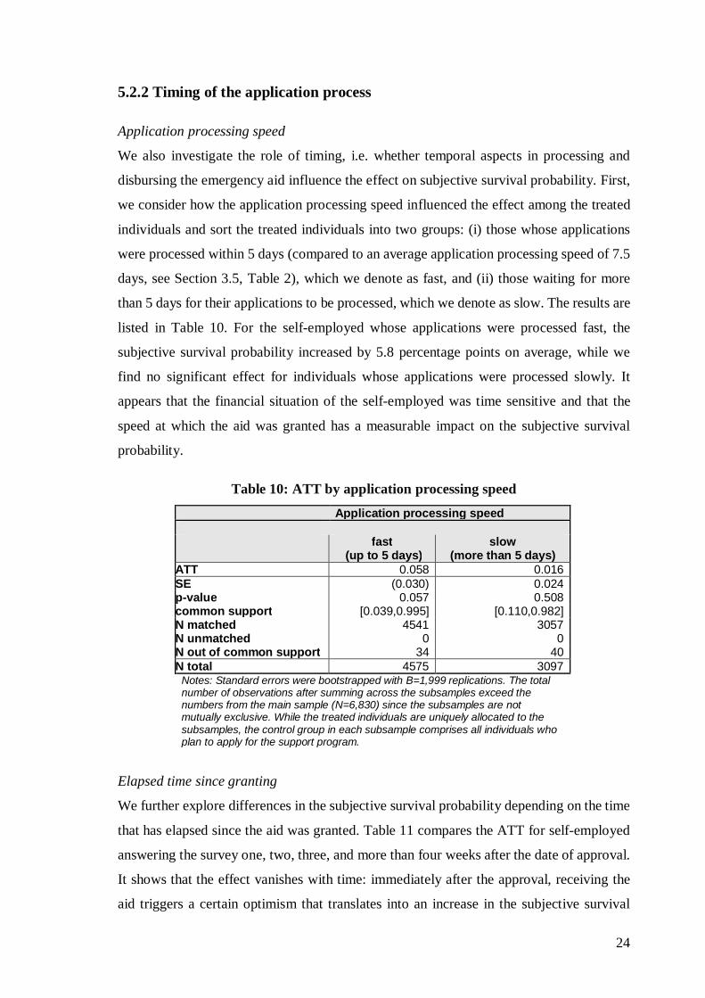
Application processing speed
We also investigate the role of timing, i.e. whether temporal aspects in processing and
disbursing the emergency aid influence the effect on subjective survival probability. First,
we consider how the application processing speed influenced the effect among the treated
individuals and sort the treated individuals into two groups: (i) those whose applications
were processed within 5 days (compared to an average application processing speed of 7.5
days, see Section 3.5, Table 2), which we denote as fast, and (ii) those waiting for more
than 5 days for their applications to be processed, which we denote as slow. The results are
listed in Table 10. For the self-employed whose applications were processed fast, the
subjective survival probability increased by 5.8 percentage points on average, while we
find no significant effect for individuals whose applications were processed slowly. It
appears that the financial situation of the self-employed was time sensitive and that the
speed at which the aid was granted has a measurable impact on the subjective survival
probability.
Table 10: ATT by application processing speed
Application processing speed
fast(up to 5 days)
slow(more than 5 days)
ATT 0.058 0.016SE (0.030) 0.024p-value 0.057 0.508common support [0.039,0.995] [0.110,0.982]N matched 4541 3057N unmatched 0 0N out of common support 34 40N total 4575 3097
Notes: Standard errors were bootstrapped with B=1,999 replications. The totalnumber of observations after summing across the subsamples exceed thenumbers from the main sample (N=6,830) since the subsamples are notmutually exclusive. While the treated individuals are uniquely allocated to thesubsamples, the control group in each subsample comprises all individuals whoplan to apply for the support program.
Elapsed time since granting
We further explore differences in the subjective survival probability depending on the time
that has elapsed since the aid was granted. Table 11 compares the ATT for self-employed
answering the survey one, two, three, and more than four weeks after the date of approval.
It shows that the effect vanishes with time: immediately after the approval, receiving the
aid triggers a certain optimism that translates into an increase in the subjective survival

25
probability of 11.2 percentage points, while the effect reduces to 8.3 percentage points after
one week and becomes insignificant after more than two weeks. The results suggest that
the program did not have a lasting effect on the financial situation of the self-employed,
probably because it consisted of a one-time payment while the financial difficulties caused
by the lockdown persisted.
Table 11: ATT by elapsed time since grantingTime elapsed since aid was granted
up to 7 days 8 to 14 days 15 to 21 days more than 21 daysATT 0.112 0.083 0.018 0.019SE (0.030) (0.026) (0.028) (0.028)p-value 0.000 0.002 0.526 0.497common support [0.031,0.865] [0.107,0.980] [0.056,0.993] [0.040,0.991]N matched 1592 2484 2580 2765N unmatched 17 9 0 0N out of common support 36 33 16 23N total 1645 2526 2596 2788
Notes: Standard errors were bootstrapped with B=1,999 replications. The total number of observations aftersumming across the subsamples exceed the numbers from the main sample (N=6,830) since the subsamplesare not mutually exclusive. While the treated individuals are uniquely allocated to the subsamples, the controlgroup in each subsample comprises all individuals who plan to apply for the support program.
5.3 Robustness Checks
5.3.1 Nearest-Neighbor-Matching
To verify whether our results are sensitive to the choice of the matching algorithm, werepeat the analysis with a propensity score based on nearest-neighbor-matching with twoneighbors and replacement. The results are listed in Table 12, columns (1) and (2), and arequite similar to those obtained under the Epanechnikov kernel estimator both in terms ofsize effect and efficiency.9 The average treatment effect amounts to 4.2 percentage pointsagainst 4.5 percentage points in the main analysis, and the average treatment effect of thetreated is 4.3 percentage points with nearest-neighbor matching against 4.4 percentagepoints in the main analysis. Apparently, using more observations from the control group asmatching partners under the kernel estimator marginally increases efficiency withoutbiasing the results. Imposing a caliper of 0.05 does not result in any further bias reductionbut leads to a higher variance since the number of potential matching partners is reduced(Table 12, columns (3) and (4)).
9 We calculate analytical standard errors following Abadie and Imbens (2016) since Abadie and Imbens(2008) show that bootstrapping does not provide consistent standard errors in the case of nearest-neighbormatching with a fixed number of neighbors and replacement. Note that trimming is less relevant withnearest-neighbor matching since only the two closest observations are used, whereas kernel matching alsouses information from faraway control units, depending on the bandwidth chosen.

26
Table 12: Nearest-Neighbor-Matching with two neighbors and replacementNN2-Matching
without trimming Caliper 0.05ATE ATT ATE ATT
treatment effect 0.042 0.043 0.043 0.041SE (0.021) (0.023) (0.022) (0.024)p-value 0.048 0.059 0.049 0.083N matched 6830 6830 6820 6820N out of common support 0 0 10 10N total 6830 6830 6830 6830
Notes: Robust standard errors were estimated following Abadie and Imbens (2016).
5.3.2 Ordinal outcome variable
The original outcome variable that we use to measure the subjective survival probability isan ordinal variable ranging from 1 (“very unlikely”) to 5 (very likely”). In the mainanalysis, we recode the variable to obtain a binary variable that can be directly interpretedas probability by setting categories 5 (“very likely”) and 4 (“rather likely”) equal to one,and the remaining categories 3 (“neutral”), 2 (“rather unlikely”), and 1 (“very unlikely”)equal to zero (see Section 4.2). To verify whether the results are sensitive to the definitionof the binary variable, we re-estimate the treatment effects with the original variable. Theresults are listed in Table 13, showing a robust positive effect both for the ATE and theATT. However, the interpretation of the magnitudes is less intuitive, as receiving financialsupport from the emergency fund increases the survival perception by 0.148 units onaverage on a scale from 1 to 5. Since the ordinal variable contains more variation acrossindividuals, the treatment effects are more efficiently estimated, supporting our conclusionthat the emergency program had a measurable effect on the self-employed persons’occupational survival probability, even though the magnitude of the effect was moderate.Table 15 in the appendix lists the results for the heterogeneity analysis, which are in linewith the binary model.
Table 13: Ordinal outcome variable
Ordinal outcome variable
ATE ATTtreatment effect 0.146 0.148
SE (0.053) (0.059)p-value 0.006 0.012common support [0.241,0.998] [0.241,0.998]N matched 6766 6766N unmatched 43 43N out of common support 21 21N total 6830 6830
Notes: Standard errors were bootstrapped with B=1,999 replications. Thepropensity score was estimated with the Epanechnikov kernel matching algorithmapplying the min-max trimming criterion. The outcome variable is the subjectiveprobability to stay self-employed during the next 12 months coded as 1 (“veryunlikely”), 2 (“likely”), 3 (“neutral”), 4 (“likely”), and 5 (“very likely”).

27
6 Discussion, Limitations, and Conclusions
The COVID-19 pandemic and the related government-mandated lock-down measures
affected the self-employed severely. As there were no existing support measures available,
many countries – including Germany - implemented on short notice financial support
programs designed to help the self-employed survive the corona crisis. In this paper, we
investigate the impact of the German emergency aid program for which €50bn was
budgeted and €13.7bn spent. The program was launched at the end of March 2020 and was
accessible for the following two months with the self-employed able to apply for a one-off
lump-sum payment of up to €15,000 to cover venture-related operating costs. In this study,
we provide first evidence on the effectiveness of this program. For our analysis, we took
advantage of a real-time online survey that was answered by more than 20,000 self-
employed individuals between April 7 and May 4, 2020, which captured a rich set of
information on variables that influence the selection into the treatment as well as the
outcome variable, namely the subjective survival probability. We use these data to
implement a propensity matching approach and compare self-employed who received the
grant with those self-employed who planned to apply for this financial support.
First of all, we observe that the applicants suffered considerable and higher monthly
financial losses than the non-applicants and lost a higher proportion of their revenue. In
this respect, the emergency aid program seems to be well targeted. Furthermore, we find
that the emergency aid program had moderate effects on the subjective probability to
remain self-employed in the subsequent months, with these positive effects appearing to
be stronger in those industries that were particularly affected by the crisis, like the event
industry, restaurants, and the tourism industry. We further reveal important heterogeneity
effects in the sense that stronger positive effects were observed among individuals who
were more risk tolerant and among higher educated self-employed, while it had no
significant effects among the self-employed with lower risk tolerance and among those
with education levels below a university degree. The latter results could be interpreted in
the sense that the more risk tolerant as well as the better educated self-employed were more
willing and more confident to make productive use of the financial support, thus also
possessing the cognitive skills needed to do so.
We also observe effects that are informative for the future design of such policy
instruments. Our real-time online survey allows for investigating the impact of the speed
of processing the application as well as how long the positive effect lasted among the
surveyed individuals. We observe that the speed in granting applications has a significant
28
impact on how helpful the financial support is perceived by the recipients. Support granted
within five days had a significant effect, while payments granted with more delay did not.
Furthermore, the positive effect of the financial support remained significant only for the
first two weeks after it was paid out; payments from the emergency aid fund that dated
back more than two weeks did not significantly affect anymore how the self-employed felt
about their prospects.
These observations are highly relevant for the further design of such policyinstruments and have three important implications: First, the program was moderatelyeffective in helping the self-employed get through the crisis. It increased their subjectivesurvival probability and, hence, their optimism to master the difficult situation. The factthat it helped some specific groups more than others may point to limitations in the use offinancial aid. As the payments could only be used to cover fixed business expenses, wespeculate that effects might have been stronger over all groups if the lump sum paymentcould have been used for covering living expenses (as was the case in various othereconomies, see Tenhagen 2020). Second, the observation that the positive effect fadedrelatively quickly allows for the interpretation that more lasting effects could have beenunleashed if the one-off lump sum payment would have been replaced with monthlypayments. Third, many evaluation studies include descriptive analyses regarding theadmission process of state-financed support instruments without being able to draw anylarger conclusions. The analysis of our real-time data set reveals that the speed of theprocess is key to the success of this financial support instrument. It clarifies how importantit is to have a well-prepared administrative structure that is able to process a large numberof applications in a relatively short period of time.
Concluding we should emphasize the main challenge of this paper, which alsoreflects its limitation. Having been able to work with such a large real-time dataset, itremains to be cross-sectional. Ideally, a panel data on self-employed would have given usthe econometrical leverage to estimate the emergency aid effects in more detail, in the longrun, and give us the possibility to match subjective and objective measures. That beingsaid, we would also have liked to use a more objective outcome measure. However, at thisstage, we are only able to use subjective survival probabilities as the COVID-19 crisis isstill ongoing and it remains widely unclear when an objective measure could be introducedto evaluate such programs. Thus, introducing subjective survival probabilities is, at thisstage, the second-best solution that has its own advantages. It also allows investigating howthe speed of an admission process influences such subjective probabilities and informs thegovernment under what conditions recipients of financial support out of the emergency aidprogram perceive such support as helpful and are optimistic about their future asentrepreneurs. After all, following Ludwig Erhard, former German Minister of Economicsand father of the German “Wirtschaftswunder”, the economy is to a large extent aboutpsychology.

29
References
Abadie, A., Imbens, G. (2008). On the failure of the bootstrap for matching estimators.Econometrica 76(6) 1537-1557.
Abadie, A., Imbens, G. (2016). Matching on the estimated propensity score.Econometrica 84(2) 781-807.
Acs, Z., Åstebro, T., Audretsch, D., & Robinson, D. T. (2016). Public policy to promoteentrepreneurship: a call to arms. Small Business Economics, 47(1), 35-51.
Adams-Prassl, A., T. Boneva, M. Golin, and C. Rauh (2020). Inequality in the impact ofthe coronavirus shock: Evidence from real time surveys. Journal of PublicEconomics 189.
Audretsch, D.B; A.S. Kritikos, and A. Schiersch (2020). Micro firms and innovation inthe service sector. Small Business Economics 55, 997–1018.
Bartik, A., M. Bertrand, Z. Cullen, E. L. Glaeser, M. Luca, and C. Stanton (2020). Howare small businesses adjusting to COVID-19? Early evidence from a survey.Becker Friedman Institute for Economics Working Paper 2020-42, University ofChicago.
Beland, l._P., Fakorede, O., and D. Mikola (2020). The short-term effect of COVID-19on self-employed workers in Canada. Technical report, 2020.
Bendell, B., Sullivan, D. & Marvel, M. (2019). A gender-aware study of self-leadershipstrategies among high-growth entrepreneurs. Journal of Small BusinessManagement 57 (1), 110-130.
Bertschek, Irene und Daniel Erdsiek (2020), Soloselbstständigkeit in der Corona-Krise,Digitalisierung hilft bei der Bewältigung der Krise, ZEW-Kurzexpertise Nr. 20-08, Mannheim
Block, J.H.; C. Fisch, and M. Hirschmann (2020): Solo self-employed and bootstrapfinancing in the COVID-19 crisis, forthcoming in Small Business Economics.
Blundell, J. and S. Machin (2020). Self-employment in the COVID-19 crisis. WorkingPaper 3, Centre of Economic Performance.
Cahuc, P. (2014). Short-time work compensation schemes and employment, IZA Worldof Labor 11.
Cassar, G. (2010). Are individuals entering self‐employment overly optimistic? Anempirical test of plans and projections on nascent entrepreneur expectations.Strategic Management Journal, 31(8), 822-840.
Caliendo, M., Fossen, F., & Kritikos, A.S. (2010). The impact of risk attitudes onentrepreneurial survival. Journal of Economic Behavior & Organization 76(1) 45-63.
Caliendo, M., Fossen, F. & Kritikos, A.S. (2014). Personality characteristics and thedecisions to become and stay self-employed. Small Business Economics 42, 787–814.
Caliendo, M. & Kopeining, S. (2008). Some practical guidance for the implementation ofpropensity score matching. Journal of Economic Surveys 22(1) 31-72.
Caliendo, M. & Kuenn, S. (2011): Start-up subsidies for the unemployed: Long-termevidence and effect heterogeneity, Journal of Public Economics 95(3-4), 311-331.
Caliendo, M. Kuenn, S. & Weissenberger, M (2016): Personality traits and the evaluationof start-up subsidies, European Economic Review 86, 87-108.

30
Crossley, T.F., Fisher, P., Low, H (2021): The heterogeneous and regressiveconsequences of COVID-19: Evidence from high quality panel data. Journal ofPublic Economics, 193(1).
Dohmen, T., Falk, A., Huffman, D., Sunde, U., Schupp, J., & Wagner, G. (2011):Individual risk attitudes: measurement, determinants, and behavioralconsequences. Journal of the European Economic Association 9(3), 522-550.
de Vries, N., Liebregts, W., & van Stel, A. (2019). Explaining entrepreneurialperformance of solo self-employed from a motivational perspective. SmallBusiness Economics, 1-14.
Fairlie, R.W. (2020). The impact of COVID-19 on small business owners: The first threemonths after social-distancing restrictions, Journal of Economics andManagement Strategy 29(4) 727-740.
Federal Ministry for Economic Affairs and Energy (2020). German governmentannounces 50 billion in emergency aid for small businesses.https://www.bmwi.de/Redaktion/ EN/Pressemitteilungen/2020/20200323-50-german-government-announces-50-billion-euros-in-emergency-aid-for-small-businesses.html, accessed 2020-10-05.
Fredriksson, P. and Johannsson, P. (2008). Dynamic treatment assignment — Theconsequences for evaluations using observational data. Journal of Business &Economic Statistics 26(4) 435-445.
Fritsch, M., Brixy, U., & Falck, O. (2006). The effect of industry, region, and time onnew business survival– A multi-dimensional analysis. Review of IndustrialOrganization 28(3) 285-306.
Gimeno, J., Folta, T. B., Cooper, A. C., & Woo, C. Y. (1997). Survival of the fittest?Entrepreneurial human capital and the persistence of underperforming firms.Administrative Science Quarterly 42(4) 750-783.
Graeber, D., Kritikos, A.S., & Seebauer, J. (2020). COVID-19: A crisis of the femaleself-employed, DIW Berlin, Discussion Paper # 1903.
Hartog, J., Van Praag, M., & Van Der Sluis, J. (2010). If you are so smart, why aren't youan entrepreneur? Returns to cognitive and social ability: entrepreneurs versusemployees. Journal of Economics & Management Strategy 19(4) 947-989.
Holtz-Eakin, D., Joulfaian, D., & Rosen, H. S. (1994). Sticking it out: entrepreneurialsurvival and liquidity constraints. Journal of Political Economy 102(1) 53-75.
Hurst, E., & Lusardi, A. (2004). Liquidity constraints, household wealth, andentrepreneurship. Journal of Political Economy, 112(2), 319-347.
Hyytinen, A., Lahtonen, J., & Pajarinen, M. (2014). Forecasting errors of new venturesurvival. Strategic Entrepreneurship Journal, 8(4), 283-302.
IfW (2020). Economic Outlook Update: German GDP expected to slump between 4.5and 9 percent in 2020. https://www.ifw-kiel.de/publications/media-information/2020/economic-outlook-update-german-gdp-expected-to-slump-between-45-and-9-percent-in-2020/ (accessed 14 April 2020).
Kalenkoski, C. M. and S. W. Pabilonia (2020). Initial impact of the COVID-19 pandemicon the employment and hours of self-employed coupled and single workers bygender and parental status. IZA Discussion Paper 13443, Bonn.
Kato, M., & Honjo, Y. (2015). Entrepreneurial human capital and the survival of newfirms in high-and low-tech sectors. Journal of Evolutionary Economics 25(5) 925-957.
Kautonen, T., Down, S., & Minniti, M. (2014). Ageing and entrepreneurial preferences.Small Business Economics 42(3) 579-594.

31
Kritikos, A.S., D. Graeber, and J. Seebauer (2020). Corona-Pandemie wird zur Krise fuerSelbstaendige. DIW aktuell 47.
Minniti, M. (2008). The role of government policy on entrepreneurial activity:productive, unproductive, or destructive? Entrepreneurship Theory and Practice,32(5), 779-790.
Parker, S. C., & Van Praag, C. M. (2006). Schooling, capital constraints, andentrepreneurial performance: The endogenous triangle. Journal of Business &Economic Statistics 24(4) 416-431.
Raffiee, J. & Feng, J. (2014). Should I quit my day job? A hybrid path toentrepreneurship Academy of Management Journal 57 (4) 936-963.
Rosenbaum, P. and Rubin, D. (1985). Constructing a control group using multivariatematched sampling methods that incorporate the propensity score. The AmericanStatistician 39(1) 33-38.
Roy, A. (1951). Some thoughts on the distribution of earnings. Oxford Economic Papers3(2) 135-145.
Rubin, D. (1974). Estimating causal effects to treatments in randomized andnonrandomized studies. Journal of Educational Psychology 66(5) 688-701.
Rubin, D. (2001). Using propensity scores to help design observational studies:application to the tobacco litigation. Health Services & Outcomes ResearchMethodology 2(3-4) 169-188.
Sianesi, B. (2004). An evaluation of the Swedish system of active labor market programsin the 1990s The Review of Economics and Statistics 89(1) 133-155.
Simón-Moya, V., Revuelto-Taboada, L., & Ribeiro-Soriano, D. (2016). Influence ofeconomic crisis on new SME survival: reality or fiction? Entrepreneurship andRegional Development 28(1): 157–176
Sorgner, A., Fritsch, M. & Kritikos, A.S. (2017): Do entrepreneurs really earn less? SmallBusiness Economics 49(2), 251-272.
Stasielowicz, L. (2020). How important is cognitive ability when adapting to changes? Ameta-analysis of the performance adaptation literature. Personality and IndividualDifferences 166(1) 110-178.
Tenhagen, H.-J. (2020). Diese Hilfen gibt es noch für Solo-Selbständige, Der Spiegel,May 16.
Van der Sluis, J., Van Praag, M., & Vijverberg, W. (2008). Education andentrepreneurship selection and performance: a review of the empirical literature.Journal of Economic Surveys 22(5) 795-841.

32
Appendix
Table 14: Summary statisticsWhole
SampleMatchedsample
Treatmentsample
ControlSample
Variables and categories % N % N % N % NRisk toleranceHigh risk tolerance 35% 6,030 37% 2529 38% 2198 32% 331Medium risk tolerance 36% 6,086 36% 2445 36% 2075 36% 370Low risk tolerance 29% 4,974 27% 1856 26% 1530 32% 326Monthly living costs (in €)Up to 500 2% 423 1% 87 1% 60 3% 27501 to 1,000 16% 2,681 14% 950 14% 787 16% 1631,001 to 1,500 26% 4,369 26% 1750 26% 1503 24% 2471,501 to 2,000 22% 3,834 24% 1630 24% 1420 20% 2102,001 to 2,500 14% 2,376 15% 1003 15% 859 14% 1442,501 to 3,000 8% 1,440 9% 614 9% 521 9% 933,001 to 3,500 5% 779 5% 328 5% 269 6% 593,501 to 4,000 3% 458 3% 184 3% 146 4% 384,001 to 4,500 1% 214 1% 102 2% 90 1% 124,501 to 5,000 2% 282 1% 101 1% 82 2% 19More than 5,000 1% 234 1% 81 1% 66 1% 15Sales decline due to pandemicNo decline or increase 2% 307 0% 31 0% 15 2% 16Up to 25% 6% 953 3% 203 3% 154 5% 4926% to 50% 13% 2,174 10% 690 9% 527 16% 16351% to 75% 17% 2,900 17% 1154 17% 977 17% 17776% to 99% 25% 4,205 28% 1940 29% 1677 26% 263100% 38% 6,551 41% 2812 42% 2453 35% 359Estimated time to insolvencyNo separate business account 26% 4,437 25% 1690 24% 1418 26% 272Already insolvent 10% 1,627 9% 628 10% 560 7% 68One month 16% 2,776 19% 1284 19% 1103 18% 181Two months 16% 2,654 17% 1177 17% 1007 17% 170Three months 15% 2,513 16% 1069 16% 909 16% 160Four to six months 12% 2,022 11% 741 11% 610 13% 131More than 6 months 6% 1,061 4% 241 3% 196 4% 45GenderMale 48% 8200 52% 3557 52% 3036 51% 521Female 52% 8811 48% 3247 47% 2750 48% 497Diverse 1% 79 0% 26 0% 17 1% 9AgeUp to 39 years 22% 3,803 24% 1611 24% 1364 24% 24740 to 49 years 28% 4,769 28% 1938 29% 1659 27% 27950 to 59 years 37% 6,298 36% 2470 36% 2110 35% 36060 years and more 13% 2,220 12% 811 12% 670 14% 141EducationOther 21% 3,584 22% 1528 23% 1337 19% 191Professional education 18% 3,087 20% 1335 20% 1164 17% 171University degree 61% 10,419 58% 3967 57% 3302 65% 665Federal stateBaden-Württemberg 10% 1,642 10% 715 10% 577 13% 138Bavaria 17% 2,843 9% 630 8% 470 16% 160Berlin 11% 1,852 19% 1313 22% 1252 6% 61Brandenburg 3% 439 2% 156 2% 139 2% 17

33
Bremen 1% 144 0% 31 0% 23 1% 8Hamburg 5% 914 6% 433 6% 354 8% 79Hesse 8% 1,344 6% 411 5% 303 11% 108Mecklenburg-Western Pomerania 1% 203 1% 49 1% 42 1% 7Lower Saxony 8% 1,295 6% 379 5% 299 8% 80North Rhine-Westphalia 21% 3,544 29% 1978 31% 1780 19% 198Rhineland Palatinate 4% 741 2% 152 2% 92 6% 60Saarland 1% 103 0% 26 0% 20 1% 6Saxony 5% 889 4% 277 4% 233 4% 44Saxony-Anhalt 1% 252 1% 54 1% 43 1% 11Schleswig-Holstein 3% 590 2% 142 2% 107 3% 35Thuringia 2% 295 1% 84 1% 69 1% 15Duration of self-employment0 to 4 years 19% 3,309 17% 1151 17% 964 18% 1875 to 10 years 25% 4,254 24% 1663 25% 1427 23% 23611 to 20 years 33% 5,648 34% 2345 34% 1984 35% 36121 to 30 years 17% 2,927 19% 1292 19% 1104 18% 188More than 30 years 6% 952 6% 379 6% 324 5% 55Industry categoryManufacturing 6% 982 6% 397 6% 334 6% 63Trade; repair of motor vehicles 2% 425 2% 162 3% 152 1% 10Accommodation and food service 2% 329 3% 172 3% 162 1% 10Information and communication 12% 2,063 10% 661 9% 538 12% 123Professional services 7% 1,277 6% 405 6% 325 8% 80Other service activities 5% 933 4% 246 3% 191 5% 55Education 12% 2,054 11% 782 11% 651 13% 131Human health and social work act. 8% 1,284 6% 439 6% 355 8% 84Arts, entertainment and recreation 41% 7,006 48% 3298 50% 2875 41% 423Other 4% 737 4% 268 4% 220 5% 48Level of digitization(continuous scale from 1 to 5)Mean (std. dev) 2.89 (1.18) 2.84 (1.16) 2.87 (1.14) 2.86 (1.14)Part-time/full-time self-employedPart-time 11% 1,845 5% 318 4% 206 11% 112Full time 89% 15,245 95% 6512 96% 5597 89% 915Solo self-employedNo 21% 3,598 24% 1640 24% 1417 22% 223Yes 79% 13,492 76% 5190 76% 4386 78% 804Application for basic security(“Hartz IV”)Not applied 92% 15,763 92% 6274 91% 5282 97% 992Applied 7% 1,225 8% 531 9% 505 3% 26Already paid out 1% 102 0% 25 0% 16 1% 9

34
Table 15: Heterogeneity analysis with ordinal outcome variableOrdinal outcome variable
ATT SE N matchedrisk attitude Low risk tolerance 0.010 (0.106) 1707 Medium risk tolerance 0.054 (0.104) 2236 high risk tolerance 0.287** (0.117) 2432education university degree 0.176** (0.075) 3895 no university degree 0.034 (0.104) 2455industry exposure to the crisis particularly affected 0.325*** (0.075) 3217 less affected 0.056 (0.094) 3024application processing speed fast (up to 5 days) 0.158** (0.078) 4541 slow (more than 5 days) 0.044 (0.061) 3057elapsed time since granting up to 7 days 0.329*** (0.074) 1645 15 to 21 days 0.084 (0.070) 2596 more than 21 days 0.067 (0.069) 2788Notes: p-values : **** p < 0.01, ** 0.01 < p < 0.05, * 0.05 < p < 0.1. Standarderrors were bootstrapped with B=1,999 replications. The propensity score wasestimated with the Epanechnikov kernel matching algorithm applying the min-max trimming criterion. The outcome variable is the subjective probability to stayself-employed during the next 12 months coded as 1 (“very unlikely”), 2 (“likely”),3 (“neutral”), 4 (“likely”), and 5 (“very likely”).