UNIT III

FUNCTION ORIENTED SOFTWARE DESIGN

SOFTWARE ANALYSIS & DESIGN TOOLS

Software analysis and design includes all activities, which help the transformation of

requirement specification into implementation. Requirement specifications specify all functional

and non-functional expectations from the software. These requirement specifications come in

the shape of human readable and understandable documents, to which a computer has nothing to

do.

Software analysis and design is the intermediate stage, which helps human-readable

requirements to be transformed into actual code.

Let us see few analysis and design tools used by software designers:

Data Flow Diagram

Data flow diagram is a graphical representation of data flow in an information system. It is

capable of depicting incoming data flow, outgoing data flow and stored data. The DFD does not

mention anything about how data flows through the system.

There is a prominent difference between DFD and Flowchart. The flowchart depicts flow of

control in program modules. DFDs depict flow of data in the system at various levels. DFD does

not contain any control or branch elements.

Types of DFD

Data Flow Diagrams are either Logical or Physical.

Logical DFD - This type of DFD concentrates on the system process and flow of data in

the system. For example in a Banking software system, how data is moved between

different entities.

Physical DFD - This type of DFD shows how the data flow is actually implemented in

the system. It is more specific and close to the implementation.

DFD Components

DFD can represent Source, destination, storage and flow of data using the following set of

components -

Fig 10.1: DFD Components

Entities - Entities are source and destination of information data. Entities are represented

by rectangles with their respective names.

Process - Activities and action taken on the data are represented by Circle or Round-

edged rectangles.

Data Storage - There are two variants of data storage - it can either be represented as a

rectangle with absence of both smaller sides or as an open-sided rectangle with only one

side missing.

Data Flow - Movement of data is shown by pointed arrows. Data movement is shown

from the base of arrow as its source towards head of the arrow as destination.

Importance of DFDs in a good software design

The main reason why the DFD technique is so popular is probably because of the fact that DFD

is a very simple formalism – it is simple to understand and use. Starting with a set of high-level

functions that a system performs, a DFD model hierarchically represents various sub-functions.

In fact, any hierarchical model is simple to understand. Human mind is such that it can easily

understand any hierarchical model of a system – because in a hierarchical model, starting with a

very simple and abstract model of a system, different details of the system are slowly introduced

through different hierarchies. The data flow diagramming technique also follows a very simple

set of intuitive concepts and rules. DFD is an elegant modeling technique that turns out to be

useful not only to represent the results of structured analysis of a software problem, but also for

several other applications such as showing the flow of documents or items in an organization.

Data Dictionary

A data dictionary lists all data items appearing in the DFD model of a system. The data items

listed include all data flows and the contents of all data stores appearing on the DFDs in the DFD

model of a system. A data dictionary lists the purpose of all data items and the definition of all

composite data items in terms of their component data items. For example, a data dictionary

entry may represent that the data grossPay consists of the components regularPay and

overtimePay.

grossPay = regularPay + overtimePay

For the smallest units of data items, the data dictionary lists their name and their type. Composite

data items can be defined in terms of primitive data items using the following data definition

operators:

+: denotes composition of two data items, e.g. a+b represents data a and b.

[,,]: represents selection, i.e. any one of the data items listed in the brackets can occur.

For example, [a,b] represents either a occurs or b occurs.

(): the contents inside the bracket represent optional data which may or may not appear.

e.g. a+(b) represents either a occurs or a+b occurs.

{}: represents iterative data definition, e.g. {name}5 represents five name data. {name}*

represents zero or more instances of name data.

=: represents equivalence, e.g. a=b+c means that a represents b and c.

/* */: Anything appearing within /* and */ is considered as a comment.

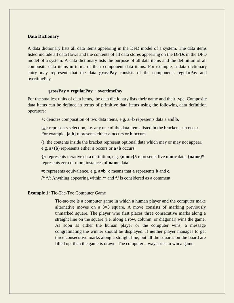
Example 1: Tic-Tac-Toe Computer Game

Tic-tac-toe is a computer game in which a human player and the computer make

alternative moves on a 3×3 square. A move consists of marking previously

unmarked square. The player who first places three consecutive marks along a

straight line on the square (i.e. along a row, column, or diagonal) wins the game.

As soon as either the human player or the computer wins, a message

congratulating the winner should be displayed. If neither player manages to get

three consecutive marks along a straight line, but all the squares on the board are

filled up, then the game is drawn. The computer always tries to win a game.

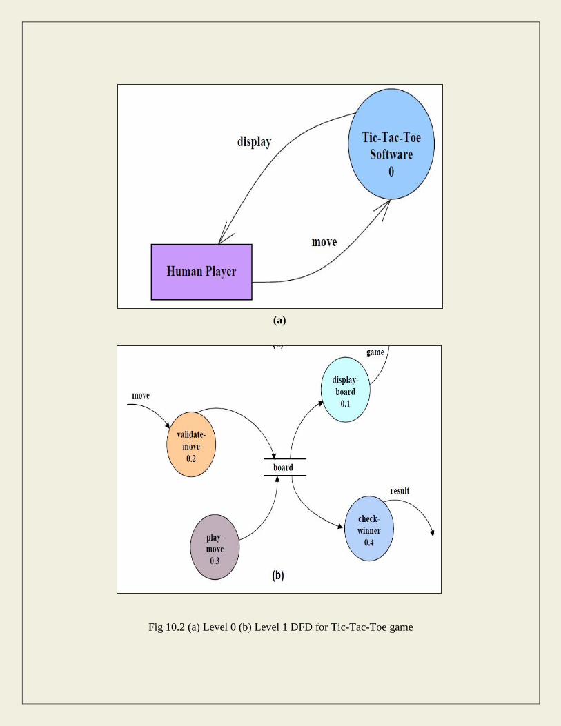
(a)

Fig 10.2 (a) Level 0 (b) Level 1 DFD for Tic-Tac-Toe game

It may be recalled that the DFD model of a system typically consists of several DFDs: level 0,

level 1, etc. However, a single data dictionary should capture all the data appearing in all the

DFDs constituting the model. Figure 10.2 represents the level 0 and level 1 DFDs for the tic-tac-

toe game. The data dictionary for the model is given below.

Data Dictionary for the DFD model in Example 1

move: integer /*number between 1 and 9 */

display: game+result

game: board

board: {integer}9

result: [“computer won”, “human won” “draw”]

Importance of Data Dictionary

A data dictionary plays a very important role in any software development process because of

the following reasons:

• A data dictionary provides a standard terminology for all relevant data for use by the

engineers working in a project. A consistent vocabulary for data items is very important,

since in large projects different engineers of the project have a tendency to use different

terms to refer to the same data, which unnecessary causes confusion.

• The data dictionary provides the analyst with a means to determine the definition of

different data structures in terms of their component elements.

Balancing a DFD

The data that flow into or out of a bubble must match the data flow at the next level of DFD. This

is known as balancing a DFD. The concept of balancing a DFD has been illustrated in fig. 10.3.

In the level 1 of the DFD, data items d1 and d3 flow out of the bubble 0.1 and the data item d2

flows into the bubble 0.1. In the next level, bubble 0.1 is decomposed. The decomposition is

balanced, as d1 and d3 flow out of the level 2 diagram and d2 flows in.

Fig. 10.3: An example showing balanced decomposition

Context Diagram

The context diagram is the most abstract data flow representation of a system. It represents the

entire system as a single bubble. This bubble is labeled according to the main function of the

system. The various external entities with which the system interacts and the data flow occurring

between the system and the external entities are also represented. The data input to the system

and the data output from the system are represented as incoming and outgoing arrows. These

data flow arrows should be annotated with the corresponding data names. The name „context

diagram‟ is well justified because it represents the context in which the system is to exist, i.e. the

external entities who would interact with the system and the specific data items they would be

supplying the system and the data items they would be receiving from the system. The context

diagram is also called as the level 0 DFD.

To develop the context diagram of the system, it is required to analyze the SRS document to

identify the different types of users who would be using the system and the kinds of data they

would be inputting to the system and the data they would be receiving the system. Here, the term

“users of the system” also includes the external systems which supply data to or receive data

from the system.

The bubble in the context diagram is annotated with the name of the software system being

developed (usually a noun). This is in contrast with the bubbles in all other levels which are

annotated with verbs. This is expected since the purpose of the context diagram is to capture the

context of the system rather than its functionality.

Example 1: RMS Calculating Software.

A software system called RMS calculating software would read three integral numbers

from the user in the range of -1000 and +1000 and then determine the root mean square

(rms) of the three input numbers and display it. In this example, the context diagram (fig.

10.4) is simple to draw. The system accepts three integers from the user and returns the

result to him.

Fig. 10.4: Context Diagram

To develop the data flow model of a system, first the most abstract representation of the problem

is to be worked out. The most abstract representation of the problem is also called the context

diagram. After, developing the context diagram, the higher-level DFDs have to be developed.

Context Diagram: - This has been described earlier.

Level 1 DFD: - To develop the level 1 DFD, examine the high-level functional requirements. If

there are between 3 to 7 high-level functional requirements, then these can be directly

represented as bubbles in the level 1 DFD. We can then examine the input data to these functions

and the data output by these functions and represent them appropriately in the diagram.

If a system has more than 7 high-level functional requirements, then some of the related

requirements have to be combined and represented in the form of a bubble in the level 1 DFD.

Such a bubble can be split in the lower DFD levels. If a system has less than three high-level

functional requirements, then some of them need to be split into their sub-functions so that we

have roughly about 5 to 7 bubbles on the diagram.

Decomposition:-

Each bubble in the DFD represents a function performed by the system. The bubbles are

decomposed into sub-functions at the successive levels of the DFD. Decomposition of a bubble

is also known as factoring or exploding a bubble. Each bubble at any level of DFD is usually

decomposed to anything between 3 to 7 bubbles. Too few bubbles at any level make that level

superfluous. For example, if a bubble is decomposed to just one bubble or two bubbles, then this

decomposition becomes redundant. Also, too many bubbles, i.e. more than 7 bubbles at any level

of a DFD makes the DFD model hard to understand. Decomposition of a bubble should be

carried on until a level is reached at which the function of the bubble can be described using a

simple algorithm.

Numbering of Bubbles:-

It is necessary to number the different bubbles occurring in the DFD. These numbers help in

uniquely identifying any bubble in the DFD by its bubble number. The bubble at the context

level is usually assigned the number 0 to indicate that it is the 0 level DFD. Bubbles at level 1 are

numbered, 0.1, 0.2, 0.3, etc, etc. When a bubble numbered x is decomposed, its children bubble

are numbered x.1, x.2, x.3, etc. In this numbering scheme, by looking at the number of a bubble

we can unambiguously determine its level, its ancestors, and its successors.

Example:-

A supermarket needs to develop the following software to encourage regular customers.

For this, the customer needs to supply his/her residence address, telephone number, and

the driving license number. Each customer who registers for this scheme is assigned a

unique customer number (CN) by the computer. A customer can present his CN to the

check out staff when he makes any purchase. In this case, the value of his purchase is

credited against his CN. At the end of each year, the supermarket intends to award

surprise gifts to 10 customers who make the highest total purchase over the year. Also, it

intends to award a 22 caret gold coin to every customer whose purchase exceeded

Rs.10,000. The entries against the CN are the reset on the day of every year after the prize

winners‟ lists are generated.

The context diagram for this problem is shown in fig. 10.5, the level 1 DFD in fig. 10.6, and the

level 2 DFD in fig. 10.7.

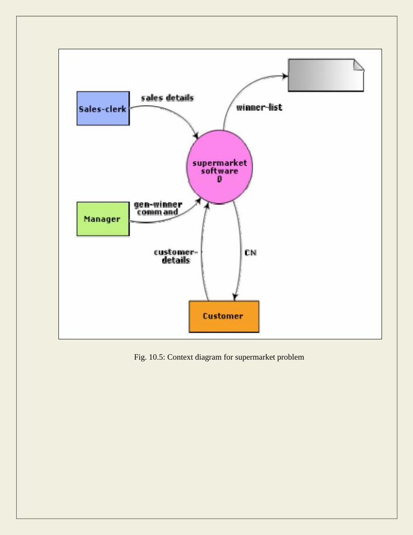
Fig. 10.5: Context diagram for supermarket problem

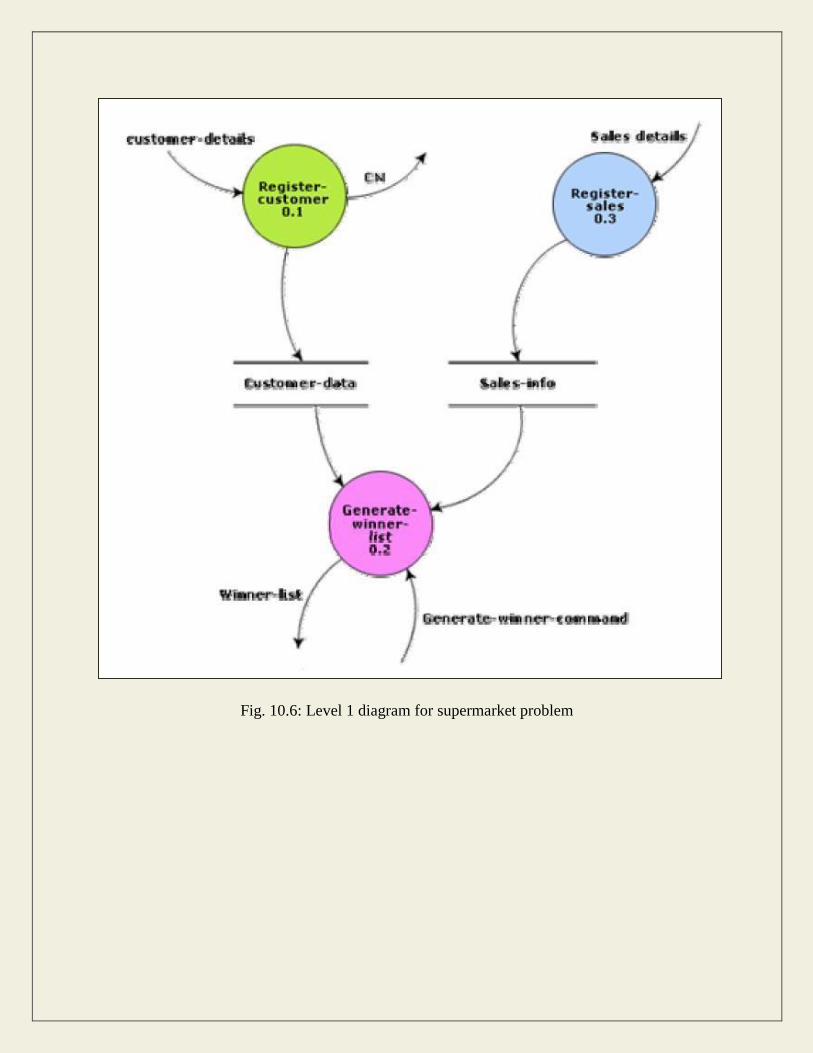
Fig. 10.6: Level 1 diagram for supermarket problem

Fig. 10.7: Level 2 diagram for supermarket problem

Example: Trading-House Automation System (TAS).

The trading house wants us to develop a computerized system that would automate

various book-keeping activities associated with its business. The following are the

salient features of the system to be developed:

• The trading house has a set of regular customers. The customers place orders with it

for various kinds of commodities. The trading house maintains the names and

addresses of its regular customers. Each of these regular customers should be

assigned a unique customer identification number (CIN) by the computer. The

customers quote their CIN on every order they place.

• Once order is placed, as per current practice, the accounts department of the trading

house first checks the credit-worthiness of the customer. The credit-worthiness of the

customer is determined by analyzing the history of his payments to different bills sent

to him in the past. After automation, this task has to be done by the computer.

• If the customer is not credit-worthy, his orders are not processed any further and an

appropriate order rejection message is generated for the customer.

• If a customer is credit-worthy, the items that have been ordered are checked against a

list of items that the trading house deals with. The items in the order which the

trading house does not deal with, are not processed any further and an appropriate

apology message for the customer for these items is generated.

• The items in the customer‟s order that the trading house deals with are checked for

availability in the inventory. If the items are available in the inventory in the desired

quantity, then

A bill with the forwarding address of the customer is printed.

A material issue slip is printed. The customer can produce this material

issue slip at the store house and take delivery of the items.

Inventory data is adjusted to reflect the sale to the customer.

If any of the ordered items are not available in the inventory in sufficient quantity to

satisfy the order, then these out-of-stock items along with the quantity ordered by the

customer and the CIN are stored in a “pending-order” file for the further processing to

be carried out when the purchase department issues the “generate indent” command.

• The purchase department should be allowed to periodically issue commands to

generate indents. When a command to generate indents is issued, the system should

examine the “pending-order” file to determine the orders that are pending and

determine the total quantity required for each of the items. It should find out the

addresses of the vendors who supply these items by examining a file containing

vendor details and then should print out indents to these vendors.

• The system should also answer managerial queries regarding the statistics of different

items sold over any given period of time and the corresponding quantity sold and the

price realized.

The context diagram for the trading house automation problem is shown in fig. 10.8, and

the level 1 DFD in fig. 10.9.

Fig. 10.8: Context diagram for TAS

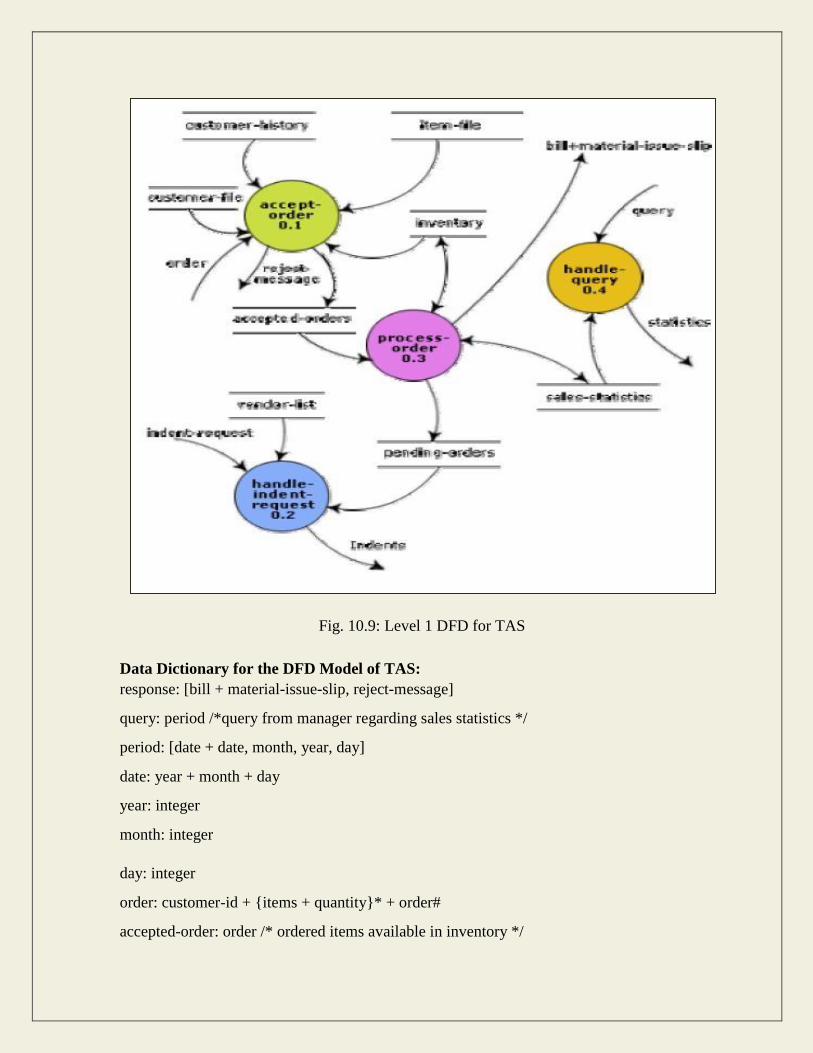
Fig. 10.9: Level 1 DFD for TAS

Data Dictionary for the DFD Model of TAS:

response: [bill + material-issue-slip, reject-message]

query: period /*query from manager regarding sales statistics */

period: [date + date, month, year, day]

date: year + month + day

year: integer

month: integer

day: integer

order: customer-id + {items + quantity}* + order#

accepted-order: order /* ordered items available in inventory */

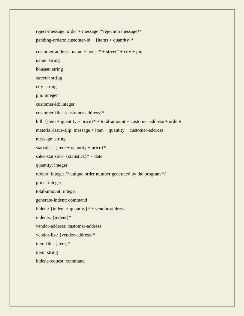
reject-message: order + message /*rejection message*/

pending-orders: customer-id + {items + quantity}*

customer-address: name + house# + street# + city + pin

name: string

house#: string

street#: string

city: string

pin: integer

customer-id: integer

customer-file: {customer-address}*

bill: {item + quantity + price}* + total-amount + customer-address + order#

material-issue-slip: message + item + quantity + customer-address

message: string

statistics: {item + quantity + price}*

sales-statistics: {statistics}* + date

quantity: integer

order#: integer /* unique order number generated by the program */

price: integer

total-amount: integer

generate-indent: command

indent: {indent + quantity}* + vendor-address

indents: {indent}*

vendor-address: customer-address

vendor-list: {vendor-address}*

item-file: {item}*

item: string

indent-request: command

Commonly made errors while constructing a DFD model

Although DFDs are simple to understand and draw, students and practitioners alike encounter

similar types of problems while modelling software problems using DFDs. While learning from

experience is powerful thing, it is an expensive pedagogical technique in the business world. It is

therefore helpful to understand the different types of mistakes that users usually make while

constructing the DFD model of systems.

Many beginners commit the mistake of drawing more than one bubble in the context

diagram. A context diagram should depict the system as a single bubble.

Many beginners have external entities appearing at all levels of DFDs. All external

entities interacting with the system should be represented only in the context diagram.

The external entities should not appear at other levels of the DFD.

It is a common oversight to have either too less or too many bubbles in a DFD. Only 3 to

7 bubbles per diagram should be allowed, i.e. each bubble should be decomposed to

between 3 and 7 bubbles.

Many beginners leave different levels of DFD unbalanced.

A common mistake committed by many beginners while developing a DFD model is

attempting to represent control information in a DFD. It is important to realize that a

DFD is the data flow representation of a system, and it does not represent control

information. For an example mistake of this kind:

Consider the following example. A book can be searched in the library catalog by

inputting its name. If the book is available in the library, then the details of the

book are displayed. If the book is not listed in the catalog, then an error message

is generated. While generating the DFD model for this simple problem, many

beginners commit the mistake of drawing an arrow (as shown in fig. 10.10) to

indicate the error function is invoked after the search book. But, this is control

information and should not be shown on the DFD.

Fig. 10.10: Showing control information on a DFD - incorrect

Another error is trying to represent when or in what order different functions (processes)

are invoked and not representing the conditions under which different functions are

invoked.

If a bubble A invokes either the bubble B or the bubble C depending upon some

conditions, we need only to represent the data that flows between bubbles A and B or

bubbles A and C and not the conditions depending on which the two modules are

invoked.

A data store should be connected only to bubbles through data arrows. A data store

cannot be connected to another data store or to an external entity.

All the functionalities of the system must be captured by the DFD model. No function of

the system specified in its SRS document should be overlooked.

Only those functions of the system specified in the SRS document should be represented,

i.e. the designer should not assume functionality of the system not specified by the SRS

document and then try to represent them in the DFD.

Improper or unsatisfactory data dictionary.

The data and function names must be intuitive. Some students and even practicing

engineers use symbolic data names such a, b, c, etc. Such names hinder understanding the

DFD model.

Shortcomings of a DFD model

DFD models suffer from several shortcomings. The important shortcomings of the DFD models

are the following:

DFDs leave ample scope to be imprecise - In the DFD model, the function performed by

a bubble is judged from its label. However, a short label may not capture the entire

functionality of a bubble. For example, a bubble named find-book-position has only

intuitive meaning and does not specify several things, e.g. what happens when some input

information are missing or are incorrect. Further, the find-book-position bubble may not

convey anything regarding what happens when the required book is missing.

Control aspects are not defined by a DFD- For instance; the order in which inputs are

consumed and outputs are produced by a bubble is not specified. A DFD model does not

specify the order in which the different bubbles are executed. Representation of such

aspects is very important for modeling real-time systems.

The method of carrying out decomposition to arrive at the successive levels and the

ultimate level to which decomposition is carried out are highly subjective and depend on

the choice and judgment of the analyst. Due to this reason, even for the same problem,

several alternative DFD representations are possible. Further, many times it is not

possible to say which DFD representation is superior or preferable to another one.

The data flow diagramming technique does not provide any specific guidance as to how

exactly to decompose a given function into its sub-functions and we have to use

subjective judgment to carry out decomposition.

11

STRUCTURED DESIGN

The aim of structured design is to transform the results of the structured analysis (i.e. a DFD

representation) into a structure chart. Structured design provides two strategies to guide

transformation of a DFD into a structure chart.

• Transform analysis

• Transaction analysis

Normally, one starts with the level 1 DFD, transforms it into module representation using either

the transform or the transaction analysis and then proceeds towards the lower-level DFDs. At

each level of transformation, it is important to first determine whether the transform or the

transaction analysis is applicable to a particular DFD. These are discussed in the subsequent sub-

sections.

Structure Chart

A structure chart represents the software architecture, i.e. the various modules making up the

system, the dependency (which module calls which other modules), and the parameters that are

passed among the different modules. Hence, the structure chart representation can be easily

implemented using some programming language. Since the main focus in a structure chart

representation is on the module structure of the software and the interactions among different

modules, the procedural aspects (e.g. how a particular functionality is achieved) are not

represented.

The basic building blocks which are used to design structure charts are the following:

Rectangular boxes: Represents a module.

Module invocation arrows: Control is passed from on one module to another

module in the direction of the connecting arrow.

Data flow arrows: Arrows are annotated with data name; named data passes

from one module to another module in the direction of the arrow.

Library modules: Represented by a rectangle with double edges.

Selection: Represented by a diamond symbol.

Repetition: Represented by a loop around the control flow arrow.

Structure Chart vs. Flow Chart

We are all familiar with the flow chart representation of a program. Flow chart is a convenient

technique to represent the flow of control in a program. A structure chart differs from a flow

chart in three principal ways:

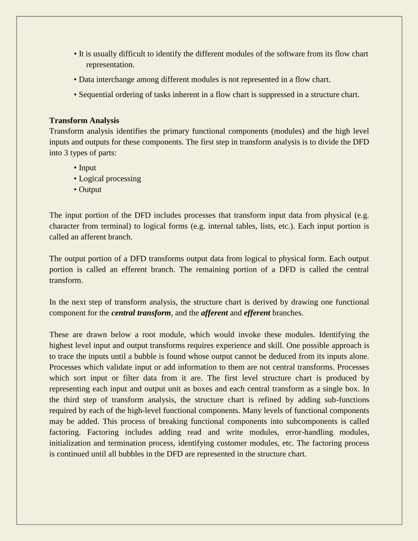
• It is usually difficult to identify the different modules of the software from its flow chart

representation.

• Data interchange among different modules is not represented in a flow chart.

• Sequential ordering of tasks inherent in a flow chart is suppressed in a structure chart.

Transform Analysis

Transform analysis identifies the primary functional components (modules) and the high level

inputs and outputs for these components. The first step in transform analysis is to divide the DFD

into 3 types of parts:

• Input

• Logical processing

• Output

The input portion of the DFD includes processes that transform input data from physical (e.g.

character from terminal) to logical forms (e.g. internal tables, lists, etc.). Each input portion is

called an afferent branch.

The output portion of a DFD transforms output data from logical to physical form. Each output

portion is called an efferent branch. The remaining portion of a DFD is called the central

transform.

In the next step of transform analysis, the structure chart is derived by drawing one functional

component for the central transform, and the afferent and efferent branches.

These are drawn below a root module, which would invoke these modules. Identifying the

highest level input and output transforms requires experience and skill. One possible approach is

to trace the inputs until a bubble is found whose output cannot be deduced from its inputs alone.

Processes which validate input or add information to them are not central transforms. Processes

which sort input or filter data from it are. The first level structure chart is produced by

representing each input and output unit as boxes and each central transform as a single box. In

the third step of transform analysis, the structure chart is refined by adding sub-functions

required by each of the high-level functional components. Many levels of functional components

may be added. This process of breaking functional components into subcomponents is called

factoring. Factoring includes adding read and write modules, error-handling modules,

initialization and termination process, identifying customer modules, etc. The factoring process

is continued until all bubbles in the DFD are represented in the structure chart.

Example: Structure chart for the RMS software

For this example, the context diagram was drawn earlier.

To draw the level 1 DFD (fig.11.1), from a cursory analysis of the problem

description, we can see that there are four basic functions that the system needs to

perform – accept the input numbers from the user, validate the numbers, calculate the

root mean square of the input numbers and, then display the result.

Fig. 11.1: Level 1 DFD

By observing the level 1 DFD, we identify the validate-input as the afferent branch and write-

output as the efferent branch. The remaining portion (i.e. compute-rms) forms the central

transform. By applying the step 2 and step 3 of transform analysis, we get the structure chart

shown in fig.11.2.

Fig. 11.2: Structure Chart

Transaction Analysis

A transaction allows the user to perform some meaningful piece of work. Transaction analysis

is useful while designing transaction processing programs. In a transaction-driven system, one

of several possible paths through the DFD is traversed depending upon the input data item.

This is in contrast to a transform centered system which is characterized by similar processing

steps for each data item. Each different way in which input data is handled is a transaction. A

simple way to identify a transaction is to check the input data. The number of bubbles on

which the input data to the DFD are incident defines the number of transactions. However,

some transaction may not require any input data. These transactions can be identified from the

experience of solving a large number of examples.

For each identified transaction, trace the input data to the output. All the traversed bubbles

belong to the transaction. These bubbles should be mapped to the same module on the

structure chart. In the structure chart, draw a root module and below this module draw each

identified transaction a module. Every transaction carries a tag, which identifies its type.

Transaction analysis uses this tag to divide the system into transaction modules and a

transaction-center module.

The structure chart for the supermarket prize scheme software is shown in fig. 11.3.

Fig. 11.3: Structure Chart for the supermarket prize scheme

MODULE 2

12

OBJECT MODELLING USING UML

Model

A model captures aspects important for some application while omitting (or abstracting) the rest.

A model in the context of software development can be graphical, textual, mathematical, or

program code-based. Models are very useful in documenting the design and analysis results.

Models also facilitate the analysis and design procedures themselves. Graphical models are very

popular because they are easy to understand and construct. UML is primarily a graphical

modeling tool. However, it often requires text explanations to accompany the graphical models.

Need for a model

An important reason behind constructing a model is that it helps manage complexity. Once

models of a system have been constructed, these can be used for a variety of purposes during

software development, including the following:

• Analysis

• Specification

• Code generation

• Design

• Visualize and understand the problem and the working of a system

• Testing, etc.

In all these applications, the UML models can not only be used to document the results but also

to arrive at the results themselves. Since a model can be used for a variety of purposes, it is

reasonable to expect that the model would vary depending on the purpose for which it is being

constructed. For example, a model developed for initial analysis and specification should be very

different from the one used for design. A model that is being used for analysis and specification

would not show any of the design decisions that would be made later on during the design stage.

On the other hand, a model used for design purposes should capture all the design decisions.

Therefore, it is a good idea to explicitly mention the purpose for which a model has been

developed, along with the model.

Unified Modeling Language (UML)

UML, as the name implies, is a modeling language. It may be used to visualize, specify,

construct, and document the artifacts of a software system. It provides a set of notations (e.g.

rectangles, lines, ellipses, etc.) to create a visual model of the system. Like any other language,

UML has its own syntax (symbols and sentence formation rules) and semantics (meanings of

symbols and sentences). Also, we should clearly understand that UML is not a system design or

development methodology, but can be used to document object-oriented and analysis results

obtained using some methodology.

Origin of UML

In the late 1980s and early 1990s, there was a proliferation of object-oriented design techniques

and notations. Different software development houses were using different notations to

document their object-oriented designs. These diverse notations used to give rise to a lot of

confusion.

UML was developed to standardize the large number of object-oriented modeling notations that

existed and were used extensively in the early 1990s. The principles ones in use were:

• Object Management Technology [Rumbaugh 1991]

• Booch‟s methodology [Booch 1991]

• Object-Oriented Software Engineering [Jacobson 1992]

• Odell‟s methodology [Odell 1992]

• Shaler and Mellor methodology [Shaler 1992]

It is needless to say that UML has borrowed many concepts from these modeling techniques.

Especially, concepts from the first three methodologies have been heavily drawn upon. UML

was adopted by Object Management Group (OMG) as a de facto standard in 1997. OMG is an

association of industries which tries to facilitate early formation of standards.

We shall see that UML contains an extensive set of notations and suggests construction of many

types of diagrams. It has successfully been used to model both large and small problems. The

elegance of UML, its adoption by OMG, and a strong industry backing have helped UML find

widespread acceptance. UML is now being used in a large number of software development

projects worldwide.

UML Diagrams

UML can be used to construct nine different types of diagrams to capture five different views of

a system. Just as a building can be modeled from several views (or perspectives) such as

ventilation perspective, electrical perspective, lighting perspective, heating perspective, etc.; the

different UML diagrams provide different perspectives of the software system to be developed

and facilitate a comprehensive understanding of the system. Such models can be refined to get

the actual implementation of the system.

The UML diagrams can capture the following five views of a system:

• User‟s view

• Structural view

• Behavioral view

• Implementation view

• Environmental view

Fig. 12.1: Different types of diagrams and views supported in UML

User’s view: This view defines the functionalities (facilities) made available by the system to

its users. The users‟ view captures the external users‟ view of the system in terms of the

functionalities offered by the system. The users‟ view is a black-box view of the system where

the internal structure, the dynamic behavior of different system components, the

implementation etc. are not visible. The users‟ view is very different from all other views in the

sense that it is a functional model compared to the object model of all other views. The users‟

view can be considered as the central view and all other views are expected to conform to this

view. This thinking is in fact the crux of any user centric development style.

Structural view: The structural view defines the kinds of objects (classes) important to the

understanding of the working of a system and to its implementation. It also captures the

relationships among the classes (objects). The structural model is also called the static model,

since the structure of a system does not change with time.

Behavioral view: The behavioral view captures how objects interact with each other to realize

the system behavior. The system behavior captures the time-dependent (dynamic) behavior of

the system.

Implementation view: This view captures the important components of the system and their

dependencies.

Environmental view: This view models how the different components are implemented on

different pieces of hardware.

13

USE CASE DIAGRAM

Use Case Model

The use case model for any system consists of a set of “use cases”. Intuitively, use cases

represent the different ways in which a system can be used by the users. A simple way to find all

the use cases of a system is to ask the question: “What the users can do using the system?” Thus

for the Library Information System (LIS), the use cases could be:

• issue-book

• query-book

• return-book

• create-member

• add-book, etc

Use cases correspond to the high-level functional requirements. The use cases partition the

system behavior into transactions, such that each transaction performs some useful action from

the user‟s point of view. To complete each transaction may involve either a single message or

multiple message exchanges between the user and the system to complete.

Purpose of use cases

The purpose of a use case is to define a piece of coherent behavior without revealing the internal

structure of the system. The use cases do not mention any specific algorithm to be used or the

internal data representation, internal structure of the software, etc. A use case typically

represents a sequence of interactions between the user and the system. These interactions consist

of one mainline sequence. The mainline sequence represents the normal interaction between a

user and the system. The mainline sequence is the most occurring sequence of interaction. For

example, the mainline sequence of the withdraw cash use case supported by a bank ATM drawn,

complete the transaction, and get the amount. Several variations to the main line sequence may

also exist. Typically, a variation from the mainline sequence occurs when some specific

conditions hold. For the bank ATM example, variations or alternate scenarios may occur, if the

password is invalid or the amount to be withdrawn exceeds the amount balance. The variations

are also called alternative paths. A use case can be viewed as a set of related scenarios tied

together by a common goal. The mainline sequence and each of the variations are called

scenarios or instances of the use case. Each scenario is a single path of user events and system

activity through the use case.

Representation of Use Cases

Use cases can be represented by drawing a use case diagram and writing an accompanying text

elaborating the drawing. In the use case diagram, each use case is represented by an ellipse with

the name of the use case written inside the ellipse. All the ellipses (i.e. use cases) of a system are

enclosed within a rectangle which represents the system boundary. The name of the system

being modeled (such as Library Information System) appears inside the rectangle.

The different users of the system are represented by using the stick person icon. Each stick

person icon is normally referred to as an actor. An actor is a role played by a user with respect to

the system use. It is possible that the same user may play the role of multiple actors. Each actor

can participate in one or more use cases. The line connecting the actor and the use case is called

the communication relationship. It indicates that the actor makes use of the functionality

provided by the use case. Both the human users and the external systems can be represented by

stick person icons. When a stick person icon represents an external system, it is annotated by the

stereotype <<external system>>.

Example 1:

Tic-Tac-Toe Computer Game

Tic-tac-toe is a computer game in which a human player and the computer make

alternative moves on a 3×3 square. A move consists of marking previously

unmarked square. The player who first places three consecutive marks along a

straight line on the square (i.e. along a row, column, or diagonal) wins the game.

As soon as either the human player or the computer wins, a message

congratulating the winner should be displayed. If neither player manages to get

three consecutive marks along a straight line, but all the squares on the board are

filled up, then the game is drawn. The computer always tries to win a game.

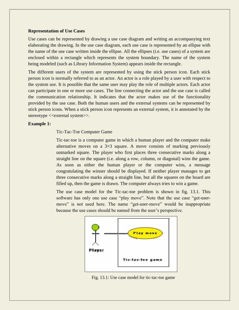
The use case model for the Tic-tac-toe problem is shown in fig. 13.1. This

software has only one use case “play move”. Note that the use case “get-user-

move” is not used here. The name “get-user-move” would be inappropriate

because the use cases should be named from the user‟s perspective.

Fig. 13.1: Use case model for tic-tac-toe game

Text Description

Each ellipse on the use case diagram should be accompanied by a text description. The text

description should define the details of the interaction between the user and the computer and

other aspects of the use case. It should include all the behavior associated with the use case in

terms of the mainline sequence, different variations to the normal behavior, the system responses

associated with the use case, the exceptional conditions that may occur in the behavior, etc. The

behavior description is often written in a conversational style describing the interactions between

the actor and the system. The text description may be informal, but some structuring is

recommended. The following are some of the information which may be included in a use case

text description in addition to the mainline sequence, and the alternative scenarios.

Contact persons: This section lists the personnel of the client organization with whom the use

case was discussed, date and time of the meeting, etc.

Actors: In addition to identifying the actors, some information about actors using this use case

which may help the implementation of the use case may be recorded.

Pre-condition: The preconditions would describe the state of the system before the use case

execution starts.

Post-condition: This captures the state of the system after the use case has successfully

completed.

Non-functional requirements: This could contain the important constraints for the design and

implementation, such as platform and environment conditions, qualitative statements, response

time requirements, etc.

Exceptions, error situations: This contains only the domain-related errors such as lack of

user‟s access rights, invalid entry in the input fields, etc. Obviously, errors that are not domain

related, such as software errors, need not be discussed here.

Sample dialogs: These serve as examples illustrating the use case.

Specific user interface requirements: These contain specific requirements for the user

interface of the use case. For example, it may contain forms to be used, screen shots, interaction

style, etc.

Document references: This part contains references to specific domain-related documents

which may be useful to understand the system operation

Example 2:

A supermarket needs to develop the following software to encourage regular

customers. For this, the customer needs to supply his/her residence address,

telephone number, and the driving license number. Each customer who registers

for this scheme is assigned a unique customer number (CN) by the computer. A

customer can present his CN to the checkout staff when he makes any purchase.

In this case, the value of his purchase is credited against his CN. At the end of

each year, the supermarket intends to award surprise gifts to 10 customers who

make the highest total purchase over the year. Also, it intends to award a 22 caret

gold coin to every customer whose purchase exceeded Rs.10,000. The entries

against the CN are the reset on the day of every year after the prize winners‟ lists

are generated.

The use case model for the Supermarket Prize Scheme is shown in fig. 13.2. As discussed

earlier, the use cases correspond to the high-level functional requirements. From the problem

description, we can identify three use cases: “register-customer”, “register-sales”, and “select-

winners”. As a sample, the text description for the use case “register-customer” is shown.

Fig. 13.2 Use case model for Supermarket Prize Scheme

Text description

U1: register-customer: Using this use case, the customer can register himself by providing the

necessary details.

Scenario 1: Mainline sequence

1. Customer: select register customer option.

2. System: display prompt to enter name, address, and telephone number.

Customer: enter the necessary values.

4. System: display the generated id and the message that the customer has been

successfully registered.

Scenario 2: at step 4 of mainline sequence

1. System: displays the message that the customer has already registered.

Scenario 2: at step 4 of mainline sequence

1. System: displays the message that some input information has not been

entered. The system displays a prompt to enter the missing value.

The description for other use cases is written in a similar fashion.

Utility of use case diagrams

From use case diagram, it is obvious that the utility of the use cases are represented by ellipses.

They along with the accompanying text description serve as a type of requirements specification

of the system and form the core model to which all other models must conform. But, what about

the actors (stick person icons)? One possible use of identifying the different types of users

(actors) is in identifying and implementing a security mechanism through a login system, so that

each actor can involve only those functionalities to which he is entitled to. Another possible use

is in preparing the documentation (e.g. users‟ manual) targeted at each category of user. Further,

actors help in identifying the use cases and understanding the exact functioning of the system.

Factoring of use cases

It is often desirable to factor use cases into component use cases. Actually, factoring of use cases

are required under two situations. First, complex use cases need to be factored into simpler use

cases. This would not only make the behavior associated with the use case much more

comprehensible, but also make the corresponding interaction diagrams more tractable. Without

decomposition, the interaction diagrams for complex use cases may become too large to be

accommodated on a single sized (A4) paper. Secondly, use cases need to be factored whenever

there is common behavior across different use cases. Factoring would make it possible to define

such behavior only once and reuse it whenever required. It is desirable to factor out common

usage such as error handling from a set of use cases. This makes analysis of the class design

much simpler and elegant. However, a word of caution here. Factoring of use cases should not

be done except for achieving the above two objectives. From the design point of view, it is not

advantageous to break up a use case into many smaller parts just for the sake of it.

UML offers three mechanisms for factoring of use cases as follows:

1. Generalization

Use case generalization can be used when one use case that is similar to another, but

does something slightly differently or something more. Generalization works the same

way with use cases as it does with classes. The child use case inherits the behavior and

meaning of the parent use case. The notation is the same too (as shown in fig. 13.3). It is

important to remember that the base and the derived use cases are separate use cases and

should have separate text descriptions.

Fig. 13.3: Representation of use case generalization

Includes

The includes relationship in the older versions of UML (prior to UML 1.1) was known as

the uses relationship. The includes relationship involves one use case including the

behavior of another use case in its sequence of events and actions. The includes

relationship occurs when a chunk of behavior that is similar across a number of use

cases. The factoring of such behavior will help in not repeating the specification and

implementation across different use cases. Thus, the includes relationship explores the

issue of reuse by factoring out the commonality across use cases. It can also be gainfully

employed to decompose a large and complex use cases into more manageable parts. As

shown in fig. 13.4 the includes relationship is represented using a predefined stereotype

<<include>>.In the includes relationship, a base use case compulsorily and automatically

includes the behavior of the common use cases. As shown in example fig. 13.5, issue-

book and renew-book both include check-reservation use case. The base use case may

include several use cases. In such cases, it may interleave their associated common use

cases together. The common use case becomes a separate use case and the independent

text description should be provided for it.

Fig. 13.4 Representation of use case inclusion

Fig. 13.5: Example use case inclusion

Extends

The main idea behind the extends relationship among the use cases is that it allows you to

show optional system behavior. An optional system behavior is extended only under certain

conditions. This relationship among use cases is also predefined as a stereotype as shown in

fig. 13.6. The extends relationship is similar to generalization. But unlike generalization, the

extending use case can add additional behavior only at an extension point only when certain

conditions are satisfied. The extension points are points within the use case where variation

to the mainline (normal) action sequence may occur. The extends relationship is normally

used to capture alternate paths or scenarios.

Fig. 13.6: Example use case extension

Organization of use cases

When the use cases are factored, they are organized hierarchically. The high-level use cases are

refined into a set of smaller and more refined use cases as shown in fig. 13.7. Top-level use

cases are super-ordinate to the refined use cases. The refined use cases are sub-ordinate to the

top-level use cases. Note that only the complex use cases should be decomposed and organized

in a hierarchy. It is not necessary to decompose simple use cases. The functionality of the super-

ordinate use cases is traceable to their sub-ordinate use cases. Thus, the functionality provided

by the super-ordinate use cases is composite of the functionality of the sub-ordinate use cases. In

the highest level of the use case model, only the fundamental use cases are shown. The focus is

on the application context. Therefore, this level is also referred to as the context diagram. In the

context diagram, the system limits are emphasized. In the top-level diagram, only those use

cases with which external users of the system. The subsystem-level use cases specify the

services offered by the subsystems. Any number of levels involving the subsystems may be

utilized. In the lowest level of the use case hierarchy, the class-level use cases specify the

functional fragments or operations offered by the classes.

Fig. 13.7: Hierarchical organization of use cases

CLASS DIAGRAMS

14

A class diagram describes the static structure of a system. It shows how a system is structured rather

than how it behaves. The static structure of a system comprises of a number of class diagrams and

their dependencies. The main constituents of a class diagram are classes and their relationships:

generalization, aggregation, association, and various kinds of dependencies.

Classes

The classes represent entities with common features, i.e. attributes and operations. Classes are

represented as solid outline rectangles with compartments. Classes have a mandatory name

compartment where the name is written centered in boldface. The class name is usually written using

mixed case convention and begins with an uppercase. The class names are usually chosen to be

singular nouns. Classes have optional attributes and operations compartments. A class may appear on

several diagrams. Its attributes and operations are suppressed on all but one diagram.

Attributes

An attribute is a named property of a class. It represents the kind of data that an object might contain.

Attributes are listed with their names, and may optionally contain specification of their type, an

initial value, and constraints. The type of the attribute is written by appending a colon and the type

name after the attribute name. Typically, the first letter of a class name is a small letter. An example

for an attribute is given.

bookName : String

Operation

Operation is the implementation of a service that can be requested from any object of the class to

affect behaviour. An object‟s data or state can be changed by invoking an operation of the object. A

class may have any number of operations or no operation at all. Typically, the first letter of an

operation name is a small letter. Abstract operations are written in italics. The parameters of an

operation (if any), may have a kind specified, which may be „in‟, „out‟ or „inout‟. An operation may

have a return type consisting of a single return type expression. An example for an operation is given.

issueBook(in bookName):Boolean

Association

Associations are needed to enable objects to communicate with each other. An association describes

a connection between classes. The association relation between two objects is called object

connection or link. Links are instances of associations. A link is a physical or conceptual connection

between object instances. For example, suppose Amit has borrowed the book Graph Theory. Here,

borrowed is the connection between the objects Amit and Graph Theory book. Mathematically, a link

can be considered to be a tuple, i.e. an ordered list of object instances. An association describes a

group of links with a common structure and common semantics. For example, consider the statement

that Library Member borrows Books. Here, borrows is the association between the class

LibraryMember and the class Book. Usually, an association is a binary relation (between two

classes). However, three or more different classes can be involved in an association. A class can have

an association relationship with itself (called recursive association). In this case, it is usually assumed

that two different objects of the class are linked by the association relationship. Association between

two classes is represented by drawing a straight line between the concerned classes.

Fig. 14.1 illustrates the graphical representation of the association relation. The name of the

association is written alongside the association line. An arrowhead may be placed on the association

line to indicate the reading direction of the association. The arrowhead should not be misunderstood

to be indicating the direction of a pointer implementing an association. On each side of the

association relation, the multiplicity is noted as an individual number or as a value range. The

multiplicity indicates how many instances of one class are associated with each other. Value ranges

of multiplicity are noted by specifying the minimum and maximum value, separated by two dots, e.g.

1.5. An asterisk is a wild card and means many (zero or more). The association of fig. 14.1 should be

read as “Many books may be borrowed by a Library Member”. Observe that associations (and links)

appear as verbs in the problem statement.

Fig. 14.1: Association between two classes

Associations are usually realized by assigning appropriate reference attributes to the classes involved.

Thus, associations can be implemented using pointers from one object class to another. Links and

associations can also be implemented by using a separate class that stores which objects of a class are

linked to which objects of another class. Some CASE tools use the role names of the association

relation for the corresponding automatically generated attribute.

Aggregation

Aggregation is a special type of association where the involved classes represent a whole-part

relationship. The aggregate takes the responsibility of forwarding messages to the appropriate parts.

Thus, the aggregate takes the responsibility of delegation and leadership. When an instance of one

object contains instances of some other objects, then aggregation (or composition) relationship exists

between the composite object and the component object. Aggregation is represented by the diamond

symbol at the composite end of a relationship. The number of instances of the component class

aggregated can also be shown as in fig. 14.2

Fig. 14.2: Representation of aggregation

Aggregation relationship cannot be reflexive (i.e. recursive). That is, an object cannot contain objects

of the same class as itself. Also, the aggregation relation is not symmetric. That is, two classes A and

B cannot contain instances of each other. However, the aggregation relationship can be transitive. In

this case, aggregation may consist of an arbitrary number of levels.

Composition

Composition is a stricter form of aggregation, in which the parts are existence-dependent on the

whole. This means that the life of the parts closely ties to the life of the whole. When the whole is

created, the parts are created and when the whole is destroyed, the parts are destroyed. A typical

example of composition is an invoice object with invoice items. As soon as the invoice object is

created, all the invoice items in it are created and as soon as the invoice object is destroyed, all

invoice items in it are also destroyed. The composition relationship is represented as a filled diamond

drawn at the composite-end. An example of the composition relationship is shown in fig. 14.3

Fig 14.3: Representation of composition

Association vs. Aggregation vs. Composition

Association is the most general (m:n) relationship. Aggregation is a stronger

relationship where one is a part of the other. Composition is even stronger than

aggregation, ties the lifecycle of the part and the whole together.

Association relationship can be reflexive (objects can have relation to itself), but

aggregation cannot be reflexive. Moreover, aggregation is anti-symmetric (If B is a

part of A, A cannot be a part of B).

Composition has the property of exclusive aggregation i.e. an object can be a part of

only one composite at a time. For example, a Frame belongs to exactly one Window

whereas in simple aggregation, a part may be shared by several objects. For example,

a Wall may be a part of one or more Room objects.

In addition, in composition, the whole has the responsibility for the disposition of all

its parts, i.e. for their creation and destruction.

in general, the lifetime of parts and composite coincides

parts with non-fixed multiplicity may be created after composite itself

parts might be explicitly removed before the death of the composite

For example, when a Frame is created, it has to be attached to an enclosing Window.

Similarly, when the Window is destroyed, it must in turn destroy its Frame parts.

Inheritance vs. Aggregation/Composition

Inheritance describes ‘is a’ / ‘is a kind of’ relationship between classes (base class - derived

class) whereas aggregation describes ‘has a’ relationship between classes. Inheritance means

that the object of the derived class inherits the properties of the base class; aggregation means

that the object of the whole has objects of the part. For example, the relation “cash payment

is a kind of payment” is modeled using inheritance; “purchase order has a few items” is

modeled using aggregation.

Inheritance is used to model a “generic-specific” relationship between classes whereas

aggregation/composition is used to model a “whole-part” relationship between classes.

Inheritance means that the objects of the subclass can be used anywhere the super class may

appear, but not the reverse; i.e. wherever we could use instances of „payment‟ in the system,

we could substitute it with instances of „cash payment‟, but the reverse cannot be done.

Inheritance is defined statically. It cannot be changed at run-time. Aggregation is defined

dynamically and can be changed at run-time. Aggregation is used when the type of the object

can change over time.

For example, consider this situation in a business system. A BusinessPartner might be a

Customer or a Supplier or both. Initially we might be tempted to model it as in Fig 14.4(a).

But in fact, during its lifetime, a business partner might become a customer as well as a

supplier, or it might change from one to the other. In such cases, we prefer aggregation

instead (see Fig 14.4(b). Here, a business partner is a Customer if it has an aggregated

Customer object, a Supplier if it has an aggregated Supplier object and a

"Customer_Supplier" if it has both. Here, we have only two types. Hence, we are able to

model it as inheritance. But what if there were several different types and combinations

thereof? The inheritance tree would be absolutely incomprehensible.

Also, the aggregation model allows the possibility for a business partner to be neither - i.e.

has neither a customer nor a supplier object aggregated with it.

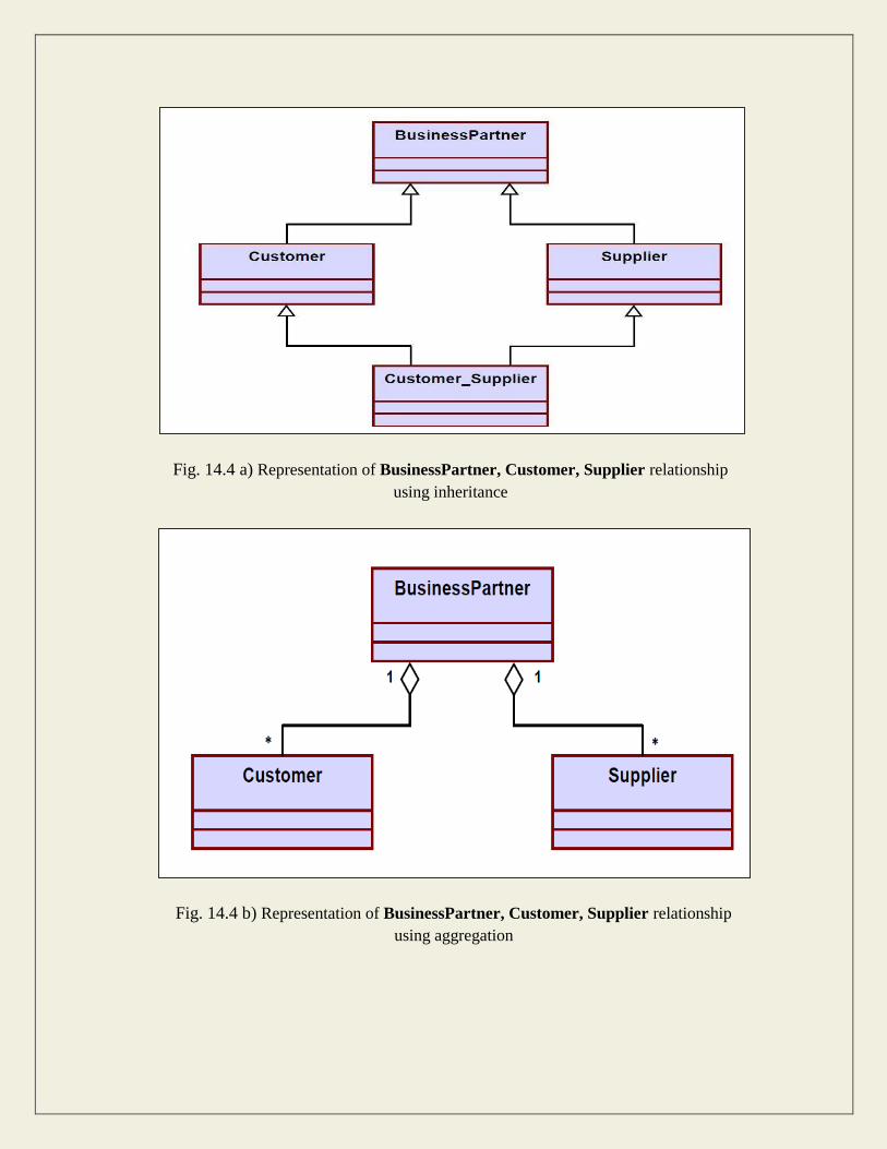
Fig. 14.4 a) Representation of BusinessPartner, Customer, Supplier relationship

using inheritance

Fig. 14.4 b) Representation of BusinessPartner, Customer, Supplier relationship

using aggregation

• The advantage of aggregation is the integrity of encapsulation. The operations of an object are the

interfaces of other objects which imply low implementation dependencies. The significant

disadvantage of aggregation is the increase in the number of objects and their relationships. On the

other hand, inheritance allows for an easy way to modify implementation for reusability. But the

significant disadvantage is that it breaks encapsulation, which implies implementation dependence.

15

INTERACTION DIAGRAMS

Interaction diagrams are models that describe how group of objects collaborate to realize some

behavior. Typically, each interaction diagram realizes the behavior of a single use case. An

interaction diagram shows a number of example objects and the messages that are passed between

the objects within the use case.

There are two kinds of interaction diagrams: sequence diagrams and collaboration diagrams. These

two diagrams are equivalent in the sense that any one diagram can be derived automatically from the

other. However, they are both useful. These two actually portray different perspectives of behavior of

the system and different types of inferences can be drawn from them. The interaction diagrams can

be considered as a major tool in the design methodology.

Sequence Diagram

A sequence diagram shows interaction among objects as a two dimensional chart. The chart is read

from top to bottom. The objects participating in the interaction are shown at the top of the chart as

boxes attached to a vertical dashed line. Inside the box the name of the object is written with a colon

separating it from the name of the class and both the name of the object and the class are underlined.

The objects appearing at the top signify that the object already existed when the use case execution

was initiated. However, if some object is created during the execution of the use case and

participates in the interaction (e.g. a method call), then the object should be shown at the appropriate

place on the diagram where it is created. The vertical dashed line is called the object‟s lifeline. The

lifeline indicates the existence of the object at any particular point of time. The rectangle drawn on

the lifetime is called the activation symbol and indicates that the object is active as long as the

rectangle exists. Each message is indicated as an arrow between the life line of two objects. The

messages are shown in chronological order from the top to the bottom. That is, reading the diagram

from the top to the bottom would show the sequence in which the messages occur. Each message is

labeled with the message name. Some control information can also be included. Two types of control

information are particularly valuable.

• A condition (e.g. [invalid]) indicates that a message is sent, only if the condition is true.

• An iteration marker shows the message is sent many times to multiple receiver objects as

would happen when a collection or the elements of an array are being iterated. The basis of

the iteration can also be indicated e.g. [for every book object].

The sequence diagram for the book renewal use case for the Library Automation Software is shown

in fig. 15.1. The development of the sequence diagram in the development methodology would help

us in determining the responsibilities of the different classes; i.e. what methods should be supported

by each class.

Fig. 15.1: Sequence diagram for the renew book use case

Collaboration Diagram

A collaboration diagram shows both structural and behavioral aspects explicitly. This is unlike a

sequence diagram which shows only the behavioral aspects. The structural aspect of a collaboration

diagram consists of objects and the links existing between them. In this diagram, an object is also

called a collaborator. The behavioral aspect is described by the set of messages exchanged among

the different collaborators. The link between objects is shown as a solid line and can be used to send

messages between two objects. The message is shown as a labeled arrow placed near the link.

Messages are prefixed with sequence numbers because they are only way to describe the relative

sequencing of the messages in this diagram. The collaboration diagram for the example of fig. 15.1

is shown in fig. 15.2. The use of the collaboration diagrams in our development process would be to

help us to determine which classes are associated with which other classes.

Fig 15.2: Collaboration diagram for the renew book use case

16

ACTIVITY AND STATE CHART DIAGRAM

The activity diagram is possibly one modeling element which was not present in any of the

predecessors of UML. No such diagrams were present either in the works of Booch, Jacobson, or

Rumbaugh. It is possibly based on the event diagram of Odell [1992] through the notation is very

different from that used by Odell. The activity diagram focuses on representing activities or chunks

of processing which may or may not correspond to the methods of classes. An activity is a state with

an internal action and one or more outgoing transitions which automatically follow the termination

of the internal activity. If an activity has more than one outgoing transitions, then these must be

identified through conditions. An interesting feature of the activity diagrams is the swim lanes. Swim

lanes enable you to group activities based on who is performing them, e.g. academic department vs.

hostel office. Thus swim lanes subdivide activities based on the responsibilities of some components.

The activities in a swim lane can be assigned to some model elements, e.g. classes or some

component, etc.

Activity diagrams are normally employed in business process modeling. This is carried out during

the initial stages of requirements analysis and specification. Activity diagrams can be very useful to

understand complex processing activities involving many components. Later these diagrams can be

used to develop interaction diagrams which help to allocate activities (responsibilities) to classes.

The student admission process in a university is shown as an activity diagram in fig. 16.1. This

shows the part played by different components of the Institute in the admission procedure. After the

fees are received at the account section, parallel activities start at the hostel office, hospital, and the

Department. After all these activities complete (this synchronization is represented as a horizontal

line), the identity card can be issued to a student by the Academic section.

Fig. 16.1: Activity diagram for student admission procedure at a university

Activity diagrams vs. procedural flow charts

Activity diagrams are similar to the procedural flow charts. The difference is that activity diagrams

support description of parallel activities and synchronization aspects involved in different activities.

STATE CHART DIAGRAM

A state chart diagram is normally used to model how the state of an object changes in its lifetime.

State chart diagrams are good at describing how the behavior of an object changes across several use

case executions. However, if we are interested in modeling some behavior that involves several

objects collaborating with each other, state chart diagram is not appropriate. State chart diagrams are

based on the finite state machine (FSM) formalism.

A FSM consists of a finite number of states corresponding to those of the object being modeled. The

object undergoes state changes when specific events occur. The FSM formalism existed long before

the object-oriented technology and has been used for a wide variety of applications. Apart from

modeling, it has even been used in theoretical computer science as a generator for regular languages.

A major disadvantage of the FSM formalism is the state explosion problem. The number of states

becomes too many and the model too complex when used to model practical systems. This problem

is overcome in UML by using state charts. The state chart formalism was proposed by David Harel

[1990]. A state chart is a hierarchical model of a system and introduces the concept of a composite

state (also called nested state).

Actions are associated with transitions and are considered to be processes that occur quickly and are

not interruptible. Activities are associated with states and can take longer. An activity can be

interrupted by an event.

The basic elements of the state chart diagram are as follows:

Initial state- This is represented as a filled circle.

Final state- This is represented by a filled circle inside a larger circle.

State- These are represented by rectangles with rounded corners.

Transition- A transition is shown as an arrow between two states. Normally, the name of the

event which causes the transition is places alongside the arrow. A guard to the transition can

also be assigned. A guard is a Boolean logic condition. The transition can take place only if

the grade evaluates to true. The syntax for the label of the transition is shown in 3 parts: event

[guard]/action.

An example state chart for the order object of the Trade House Automation software is shown in fig.

16.2.