Unit Commitment and Economic Model Predictive Control for ... · Unit Commitment and Economic Model...
160
Unit Commitment and Economic Model Predictive Control for Optimal Operation of Power Systems Peter Juhler Dinesen, s093053 M.Sc. Thesis, February 2015
Transcript of Unit Commitment and Economic Model Predictive Control for ... · Unit Commitment and Economic Model...
Unit Commitment andEconomic Model Predictive Control forOptimal Operation of Power Systems
Peter Juhler Dinesen, s093053M.Sc. Thesis, February 2015

DTU ComputeDepartment of Applied Mathematics and Computer ScienceTechnical University of Denmark
MatematiktorvetBuilding 303BDK-2800 Kongens Lyngby, DenmarkPhone +45 4525 [email protected]

AbstractThis thesis focuses on combining the Unit Commitment (UC) optimization problemand the economic Model Predictive Control (MPC) problem for optimal operation ofpower systems. The growing uncertainty associated with the increasing share of inter-mittent renewable energy sources in the power supply has presented new challengesfor optimal operation of power systems. Motivated by these challenges, we present anovel control strategy that shows capability of managing uncertainty with flexibility.
The proposed hierarchy control structure consists of two-levels:
• Apply UC to determine which power plants are running as well as the maindistribution of power production.
• Apply economic MPC to repeatedly reoptimize the production in a recedinghorizon manner while considering updated and more reliable forecasts of powersupply from renewable energy sources.
We mathematically formalize the UC as a mixed integer linear programming problemand the control problem as a soft constrained linear economic MPC optimization prob-lem. Deterministic and stochastic formulations are provided, as well as disturbancemodeling for offset free MPC.
The developed control strategy is tested on a power system consisting of a portfolio ofcontrollable power plants and non-controllable farms of wind turbines. The results ofthe simulations successfully show that the novel control strategy appears to providea feasible and a promising solution to overcome some of the important challenges.Furthermore, it show that the economic MPC method play an important role in thecontrol of optimal power system operations. We demonstrate significant savings inimbalance cost and potential reduction in the need of the expensive spinning reserve.
Additionally, results indicate that the coarse discretization and the input param-eterization for the UC have a cost impact on the solution. Solving the UC problemwith high resolution yields the optimal production plan. Comparing to the optimalproduction plan, the UC solution with coarse discretization obtain 2.63% imbalancepower while the economic MPC solution coincide with the optimal production plan.Simultaneous, the runtime for the economic MPC is 65x faster than solving the UCwith high resolution.

ii

ResuméDenne afhandling fokuserer på at sammenkoble Unit Commitment (UC) optimer-ingsproblem og økonomisk model prædiktiv regulering (MPC) for optimal styring afenergisystemer. Energiforsyning fra vedvarende energikilder er varierende. Dermedopstår der nye udfordringer for at opretholde optimal drift og styring af energisyste-mer, nå disse energikilder udgør en større andel i det samlede forsyningsnet. Motiveretaf disse udfordringer, præsenterer vi en innovativ kontrolstrategi.
Den forslåede kontrolstrategi består af to niveauer:
• Anvende UC til at bestemme, hvilke kraftværker der skal være tændt samtfordeling af energiproduktionen på disse.
• Anvende økonomisk MPC for gentagne gange at optimere produktionen, re-altidsoptimering, med rullende horisont. Her tages opdateret og mere pålideligeprognoser for strømforsyning fra vedvarende energikilder i betragtning.
Vi formulerer matematisk UC som et blandet heltal lineært programmeringsproblemog reguleringsproblemet som et som et blødt begrænsede lineært økonomisk MPC op-timeringsproblem. Vi præsenterer deterministiske og stokastiske formuleringer, samtmodellere forstyrrelser for at opnå offset-free MPC.
Den udviklede kontrolstrategien testes på et energisystem bestående af en portefølje afstyrbare kraftværker og ikke-styrbare vindmølle farm. Resultaterne af simuleringerneindikere at kontrolstrategien er en yderst lovende løsning til nogle af de vigtige udfor-dringer. Vi ser endvidere, at økonomisk MPC spiller en vigtig rolle i planlægning ogrealtidsoptimering til styring af energisystemer. Vi demonstrerer væsentlige bespar-elser i ubalanceomkostninger og potentiel reduktion i behovet for dyre reserver.
Derudover viser resultaterne, at den grove diskretisering og input parametriseringfor UC har en omkostning på den opnåelige løsning. Den optimale produktionsplanopnås ved løsning af UC på fin tidsskala. Sammenlignet med den optimale produktion-splan, resultere UC løsningen på grov tidsskala 2,63% ubalance imens den økonomiskeMPC løsning følger den optimale produktionsplan. Samtidigt finder økonomisk MPCløsningen 65 gange hurtigere end at løse UC på fin tidsskala.

iv

PrefaceThis thesis is submitted to the Technical University of Denmark (DTU) in partial ful-fillment of the requirements for acquiring the Master of Science (M.Sc.) Elite degreein Industrial Mathematics. The elite program is an honors program for high per-forming students. The work reported in this thesis is conducted at the Departmentof Applied Mathematics and Computer Science (DTU Compute) at the TechnicalUniversity of Denmark with Associate Professor John Bagterp Jørgensen as supervi-sor. The study and reporting is conducted in the period July 2014 to February 2015,having a workload of 30 ECTS points.
This thesis investigates the opportunity of combining the unit commitment optimiza-tion problem and the economic model predictive control problem for optimal opera-tion of power systems. An intelligent control strategy that can manage the uncertaintyassociated with the increasing share of intermittent renewable energy sources in thepower supply has presented new challenges for optimal operation of power systems.The thesis is accomplished in close collaboration with DONG Energy and the Tech-nical University of Denmark. Our contributions, value creation, and experiences arerelevant to both industry and academia.
We chose this project motivated by its topicality and its potential to be a verychallenging and ambitious project. The project proved to be very challenging andfar more comprehensive than initial expected. I am very curious by nature and findnon-trivial problem highly interesting, thus, this thesis turned out to be exactly whatI had hoped for.
The thesis consists of this report and a source code booklet, where the developedimplementations are listed.
Kgs. Lyngby, February 2015
Peter Juhler Dinesens093053

vi

AcknowledgementsFirst and foremost, I would like to express my gratitude to my supervisor AssociateProfessor John Bagterp Jørgensen to arouse my curiosity to numerical optimization,optimal control, and to the model predictive control discipline. The excellent men-toring and fruitful discussions made this experience extremely satisfying.
I would also like to thank Industrial Ph.D. student Leo Emil Sokoler for excellentguidance and for being at disposal when questions occurred.
I am utmost grateful for this.

viii

ContentsAbstract i
Resumé iii
Preface v
Acknowledgements vii
Contents ix
List of Figures xiii
List of Tables xvii
I Introduction and Background 1
1 Introduction 31.1 Global energy challenges . . . . . . . . . . . . . . . . . . . . . . . . . . 31.2 Power production planning . . . . . . . . . . . . . . . . . . . . . . . . 41.3 Unit commitment . . . . . . . . . . . . . . . . . . . . . . . . . . . . . . 51.4 Model predictive control . . . . . . . . . . . . . . . . . . . . . . . . . . 61.5 Thesis statement . . . . . . . . . . . . . . . . . . . . . . . . . . . . . . 71.6 Thesis contributions . . . . . . . . . . . . . . . . . . . . . . . . . . . . 71.7 Previous work . . . . . . . . . . . . . . . . . . . . . . . . . . . . . . . . 81.8 Thesis structure . . . . . . . . . . . . . . . . . . . . . . . . . . . . . . . 8
2 Power Systems 112.1 Power grid . . . . . . . . . . . . . . . . . . . . . . . . . . . . . . . . . . 112.2 Renewable energy sources . . . . . . . . . . . . . . . . . . . . . . . . . 132.3 Control hierarchy . . . . . . . . . . . . . . . . . . . . . . . . . . . . . . 142.4 Electricity market . . . . . . . . . . . . . . . . . . . . . . . . . . . . . 15
2.4.1 Day-ahead market . . . . . . . . . . . . . . . . . . . . . . . . . 162.4.2 Intraday market . . . . . . . . . . . . . . . . . . . . . . . . . . 16

x Contents
3 Software 173.1 IBM® ILOG® CPLEX® Optimization Studio . . . . . . . . . . . . . . . 173.2 Matlab® MathWorks® . . . . . . . . . . . . . . . . . . . . . . . . . . . 17
II Theory 19
4 Unit Commitment 214.1 Introduction . . . . . . . . . . . . . . . . . . . . . . . . . . . . . . . . . 214.2 Mathematical problem formulation . . . . . . . . . . . . . . . . . . . . 22
4.2.1 Objective function . . . . . . . . . . . . . . . . . . . . . . . . . 224.2.2 Constraints . . . . . . . . . . . . . . . . . . . . . . . . . . . . . 23
4.3 The UC optimization problem . . . . . . . . . . . . . . . . . . . . . . . 264.4 Implementation . . . . . . . . . . . . . . . . . . . . . . . . . . . . . . . 274.5 Solution methods . . . . . . . . . . . . . . . . . . . . . . . . . . . . . . 284.6 Case study . . . . . . . . . . . . . . . . . . . . . . . . . . . . . . . . . 29
4.6.1 3-unit power system . . . . . . . . . . . . . . . . . . . . . . . . 294.6.2 10-unit power system . . . . . . . . . . . . . . . . . . . . . . . 30
4.7 Summary . . . . . . . . . . . . . . . . . . . . . . . . . . . . . . . . . . 35
5 Models for Predictive Control 375.1 Modeling dynamical systems . . . . . . . . . . . . . . . . . . . . . . . 375.2 Modeling power systems . . . . . . . . . . . . . . . . . . . . . . . . . . 39
5.2.1 Power system dynamics . . . . . . . . . . . . . . . . . . . . . . 395.2.2 Discrete-time state-space model formulation . . . . . . . . . . . 415.2.3 Distributed independent power system . . . . . . . . . . . . . . 42
5.3 Finite impulse response . . . . . . . . . . . . . . . . . . . . . . . . . . 435.4 Kalman filtering and prediction . . . . . . . . . . . . . . . . . . . . . . 455.5 Disturbance modeling for offset-free MPC . . . . . . . . . . . . . . . . 475.6 Summary . . . . . . . . . . . . . . . . . . . . . . . . . . . . . . . . . . 48
6 Economic Model Predictive Control 496.1 Introduction . . . . . . . . . . . . . . . . . . . . . . . . . . . . . . . . . 496.2 Mathematical problem formulation . . . . . . . . . . . . . . . . . . . . 516.3 The economic MPC formulation . . . . . . . . . . . . . . . . . . . . . 52
6.3.1 Stability . . . . . . . . . . . . . . . . . . . . . . . . . . . . . . . 536.4 Solving the economic MPC problem . . . . . . . . . . . . . . . . . . . 55
6.4.1 Economic MPC formulated as LP problem . . . . . . . . . . . 556.4.2 Solvers . . . . . . . . . . . . . . . . . . . . . . . . . . . . . . . . 576.4.3 Optimality conditions . . . . . . . . . . . . . . . . . . . . . . . 57
6.5 Implementation . . . . . . . . . . . . . . . . . . . . . . . . . . . . . . . 576.6 Case study . . . . . . . . . . . . . . . . . . . . . . . . . . . . . . . . . 60
6.6.1 2-unit power system . . . . . . . . . . . . . . . . . . . . . . . . 606.7 Summary . . . . . . . . . . . . . . . . . . . . . . . . . . . . . . . . . . 61

Contents xi
III Unit Commitment and Economic Model Predicetive Control forPower Systems 65
7 Introduction 677.1 Developed control strategy . . . . . . . . . . . . . . . . . . . . . . . . . 677.2 Considerations for combining UC and economic MPC . . . . . . . . . 687.3 Background for the simulations . . . . . . . . . . . . . . . . . . . . . . 70
7.3.1 Demand load . . . . . . . . . . . . . . . . . . . . . . . . . . . . 707.3.2 Operational parameters . . . . . . . . . . . . . . . . . . . . . . 72
8 Discretization and Parameterization 758.1 Discretization . . . . . . . . . . . . . . . . . . . . . . . . . . . . . . . . 758.2 Parameterization . . . . . . . . . . . . . . . . . . . . . . . . . . . . . . 788.3 Key findings . . . . . . . . . . . . . . . . . . . . . . . . . . . . . . . . . 78
9 Deterministic Simulations 799.1 MISO simulations . . . . . . . . . . . . . . . . . . . . . . . . . . . . . 799.2 MIMO simulations . . . . . . . . . . . . . . . . . . . . . . . . . . . . . 85
9.2.1 System power output limits as trajectory . . . . . . . . . . . . 859.2.2 Individual production plans as trajectory . . . . . . . . . . . . 88
9.3 Key findings . . . . . . . . . . . . . . . . . . . . . . . . . . . . . . . . . 91
10 Stochastic Simulations 9310.1 Modeling forecasts of wind power supply . . . . . . . . . . . . . . . . . 9310.2 Step wind power . . . . . . . . . . . . . . . . . . . . . . . . . . . . . . 94
10.2.1 Case 1 . . . . . . . . . . . . . . . . . . . . . . . . . . . . . . . . 9410.2.2 Case 2 . . . . . . . . . . . . . . . . . . . . . . . . . . . . . . . . 96
10.3 Fluctuating wind power . . . . . . . . . . . . . . . . . . . . . . . . . . 9810.3.1 Case 1 . . . . . . . . . . . . . . . . . . . . . . . . . . . . . . . . 9910.3.2 Case 2 . . . . . . . . . . . . . . . . . . . . . . . . . . . . . . . . 10110.3.3 Case 3 . . . . . . . . . . . . . . . . . . . . . . . . . . . . . . . . 10410.3.4 Case 4 . . . . . . . . . . . . . . . . . . . . . . . . . . . . . . . . 104
10.4 Key findings . . . . . . . . . . . . . . . . . . . . . . . . . . . . . . . . . 105
IV Conclusions and Perspectives 109
11 Conclusions and Perspectives 11111.1 UC . . . . . . . . . . . . . . . . . . . . . . . . . . . . . . . . . . . . . . 11211.2 Economic MPC . . . . . . . . . . . . . . . . . . . . . . . . . . . . . . . 11211.3 UC and economic MPC . . . . . . . . . . . . . . . . . . . . . . . . . . 11211.4 Perspectives and further research . . . . . . . . . . . . . . . . . . . . . 114

xii Contents
V Appendices 115
A Background Material 117A.1 Linearization and discretization . . . . . . . . . . . . . . . . . . . . . . 117
A.1.1 Continuous-time state-space model . . . . . . . . . . . . . . . . 117A.1.2 Continuous-time transfer function . . . . . . . . . . . . . . . . 118A.1.3 Discrete-time state-space model . . . . . . . . . . . . . . . . . . 119
A.2 List of used theorems . . . . . . . . . . . . . . . . . . . . . . . . . . . . 121A.2.1 Propositional logic . . . . . . . . . . . . . . . . . . . . . . . . . 121A.2.2 Laplace transform . . . . . . . . . . . . . . . . . . . . . . . . . 121A.2.3 Z-transform . . . . . . . . . . . . . . . . . . . . . . . . . . . . . 121
B System Data 123
C The GRANI Program 127
Nomenclature 129
Bibliography 133

List of Figures1.1 Control strategy of combining the UC and the economic MPC. . . . . . . 5
2.1 Europe Brent Crude Oil Spot Price FOB in Dollars per Barrel; source U.S.Energy Information Administration (EIA) [EIA14]. . . . . . . . . . . . . . 12
2.2 Distribution of electricity consumption by source of energy in 2010 and2020 [MD12]. . . . . . . . . . . . . . . . . . . . . . . . . . . . . . . . . . . 14
2.3 Control hierarchy. . . . . . . . . . . . . . . . . . . . . . . . . . . . . . . . 152.4 The considered wind power production forecasts on the tow levels: days-
hours level and minute level. . . . . . . . . . . . . . . . . . . . . . . . . . 16
3.1 Simplified illustration of IBM ILOG CPLEX Optimization Studio. . . . . 18
4.4 24-hour demand load for the 10-unit power system [MW]. . . . . . . . . . 304.5 The optimal power production plan for each plants (blue line) with each
plants minimum and maximum power output (red dashed line). . . . . . . 314.6 The optimal power production plan for plant 1 with its minimum and
maximum power output limits. . . . . . . . . . . . . . . . . . . . . . . . . 324.7 The total production plan (dotted yellow) satisfy demand load (solid blue);
coincide throughout planning horizon. The actual spinning reserve (dottedcyan) obey the required spinning reserve (dotted red). . . . . . . . . . . . 32
4.8 Change in power output for each time step (solid blue) with each plantramping limits (dotted red). . . . . . . . . . . . . . . . . . . . . . . . . . . 33
4.9 The total production cost (solid black) over the planning horizon. Thevariable cost (dotted blue), the fixed cost (dotted red), and startup andshutdown cost (dotted cyan). . . . . . . . . . . . . . . . . . . . . . . . . . 33
4.10 Distribution of the four cost components in the objective function. . . . . 34
5.1 A generic stochastic input-output model. . . . . . . . . . . . . . . . . . . 385.2 State-space model realization of linear time-invariant models. . . . . . . . 385.3 Deterministic step responses of the transfer functions (5.5) and (5.6) dis-
cretized using zero-order hold with sampling time of Ts = 20 seconds. . . 405.4 Power grid with two controllable conventional power plants and one non-
controllable predictable power generator, farms of wind turbines. . . . . . 44

xiv List of Figures
6.1 Control principle of MPC scheme - moving horizon estimation [Wik]. . . . 506.2 A MPC system [PJ08]. . . . . . . . . . . . . . . . . . . . . . . . . . . . . . 506.3 Flowchart of developed Matlab implementation. . . . . . . . . . . . . . . 596.5 Open-loop simulation of a power system without regularization term for
excessive movement of the input. Ts = 1. . . . . . . . . . . . . . . . . . . 626.6 Open-loop simulation of a power system with regularization term for ex-
cessive movement of the input. Ts = 1. . . . . . . . . . . . . . . . . . . . . 636.7 Closed-loop economic MPC simulation of a power system. Prediction
horizon is N = 50 time step with regularization term. Ts = 1. . . . . . . . 64
7.1 Control strategy of combining the UC and the economic MPC. . . . . . . 697.2 Power system with two controllable conventional power plants and a non-
controllable predictable power generator, farms of wind turbines. . . . . . 707.3 24-hour demand load [MW]; see Table B.1(a) in Appendix B for the nu-
merical representation. Spinning reserve is 10% of demand load for eachtime period. . . . . . . . . . . . . . . . . . . . . . . . . . . . . . . . . . . . 71
8.1 Power production obtained from UCth, UCtc, and EMPCth. . . . . . . . . 76
9.1 24-hour MISO closed-loop simulation applying the busy demand load astrajectory. UC production profile for power plants are unknown whilecommitted plants are known for the economic MPC. . . . . . . . . . . . . 81
9.2 24-hour MISO closed-loop simulation applying the busy demand load. Per-formed inputs to the system and the rate of movement together with theirlimits. . . . . . . . . . . . . . . . . . . . . . . . . . . . . . . . . . . . . . . 82
9.3 24-hour MISO closed-loop simulation applying the idle demand load astrajectory. UC production profile for power plants are unknown whilecommitted plants are known for the economic MPC. . . . . . . . . . . . . 83
9.4 24-hour MISO closed-loop simulation applying the idle demand load. Per-formed inputs to the system and the rate of movement together with theirlimits. . . . . . . . . . . . . . . . . . . . . . . . . . . . . . . . . . . . . . . 84
9.5 24-hour MIMO closed-loop simulation applying the busy demand loadand system power output limits as trajectories. UC production profilefor power plants are unknown while committed plants are known for theeconomic MPC. . . . . . . . . . . . . . . . . . . . . . . . . . . . . . . . . . 86
9.6 24-hour MIMO closed-loop simulation applying the idle demand load andsystem power output limits as trajectories. UC production profile forpower plants are unknown while committed plants are known for the eco-nomic MPC. . . . . . . . . . . . . . . . . . . . . . . . . . . . . . . . . . . 87
9.7 24-hour MIMO closed-loop simulation applying the busy demand load.The economic MPC is to obey obtained production plan from solving theUC problem within a defined range (trajectories). . . . . . . . . . . . . . . 89

List of Figures xv
9.8 24-hour MIMO closed-loop simulation applying the idle demand load. Theeconomic MPC is to obey obtained production plan from solving the UCproblem within a defined range (trajectories). . . . . . . . . . . . . . . . . 90
10.1 6-hour closed-loop simulation when 150 MW wind power entering the sys-tem at hour 3. . . . . . . . . . . . . . . . . . . . . . . . . . . . . . . . . . 95
10.2 6-hour closed-loop simulation with the busy demand load. Figure 10.2(a)shows the result of offset MPC simulation and Figure 10.2(b) shows theresult of offset free MPC. Both with same simulation setup. . . . . . . . . 97
10.3 24-hour demand load [MW]. Coarse grid demand load (tc) applied in theUC problem (solid blue) and high resolution demand load (th) applied inthe economic MPC (solid cyan). Spinning reserve is 10% of demand loadtcfor each time period. . . . . . . . . . . . . . . . . . . . . . . . . . . . . . . 98
10.4 Example illustration of (10.1) applying (10.2). . . . . . . . . . . . . . . . 9910.6 6-hour closed-loop simulation. Top: Total power production from the UC
and the economic MPC. Required power generated by plants (solid red).Bottom: Wind power production defined as (10.1). . . . . . . . . . . . . . 100
10.7 Imbalance as function of time for simulation Figure 10.6. Calculated asthe differences between the optimal required power production by plantsand the two derived solutions: UC solution and economic MPC solution. . 101
10.9 24-hour closed-loop simulation with two different amplitude values. Top:Total power production from the UC and the economic MPC. Requiredpower generated by plants (solid red). Bottom: Wind power productiondefined as (10.1). . . . . . . . . . . . . . . . . . . . . . . . . . . . . . . . . 103
10.116-hour closed-loop simulation. Fixed amplitude and vary frequency. Windpower modeled by (10.2) using parameters listed in Table 10.10. . . . . . 106
10.12Same simulation as Figure 10.11(b) with the change of power output rangeto be ±0.03% of the demand load. . . . . . . . . . . . . . . . . . . . . . . 107
10.136-hour closed-loop simulation. Consider the stochastic model with stochas-tic process noise and measurements noise distributed as (10.3). . . . . . . 108
A.1 Input-ouput relation describing the transfer functions. . . . . . . . . . . . 118

xvi

List of Tables4.1 3-hour demand load for the 3-unit power system [MW]. . . . . . . . . . . 294.2 Operational parameters for the 3-unit power system. . . . . . . . . . . . . 294.3 Optimal production plan for the 3-unit power system [MW]. . . . . . . . . 30
6.4 Operational parameters. . . . . . . . . . . . . . . . . . . . . . . . . . . . . 60
7.4 Operational parameters to the UC problem. . . . . . . . . . . . . . . . . . 727.5 Operational parameters to the economic MPC. Penalty ρi,k = [ρ1,k,ρ2,k,ρT,k] =
[10,10,100], where i = 1,2, . . . ,nu and ρT,k is the penalty associated to theoverall demand load. . . . . . . . . . . . . . . . . . . . . . . . . . . . . . . 73
8.2 Results of 12-hour closed-loop simulation. Total power production [MWh]by the tree methods. Imbalance [MWh] is the absolute imbalance betweenUCth and the obtained production plan. . . . . . . . . . . . . . . . . . . . 77
10.5 Applied parameters in Figure 10.6 to (10.2). . . . . . . . . . . . . . . . . . 10010.8 Results of 24-hour closed-loop with four different amplitudes. Imbalance is
the absolute imbalance between the optimal production and the obtainedproduction plan. . . . . . . . . . . . . . . . . . . . . . . . . . . . . . . . . 101
10.10Applied parameters in Figure 10.11(a) and Figure 10.11(b) to (10.2). . . . 104
B.1 24-hour demand load [MW] applied in simulations. Spinning reserve is10% of demand load for each time period. . . . . . . . . . . . . . . . . . . 124
B.2 Operational parameters for the 10-unit power system. . . . . . . . . . . . 125

xviii

Part IIntroduction and
Background


CHAPTER 1Introduction
In this chapter, we bring the project into a context by outlining the challenges anddirections from the global energy systems that motivate our work. We address theneed for a new control strategy when introducing large amounts of intermittent re-newable energy sources into the power grid. The used methods are briefly described.Additionally, we describe the thesis statement, the contributions of our work, andprevious work. Lastly, an outline for the remainder of this thesis is given.
1.1 Global energy challenges
Energy is of paramount importance for a modern society. It has a great impact on ev-erything we do like water delivery, food, internet, computer systems, communicationsystems, etc. Major breakdowns in power systems are a fundamental concern, since itwould lead to an almost complete chaos in the Western countries. Simultaneously, weare in a global race for energy sources. Fossil fuels continue to dominate the world’senergy supplies, counting for more than 80% of energy demand [EIAa; Eur13; Off13].As we know, this energy supply is unsustainable and causing potentially catastrophicclimate change, and horrendous pollution. The world is facing global energy challengeof
• satisfy the increasing energy demands,
• ensure adequate energy sources, and
• reduce climate changes and pollution.
In the global race for energy sources and for meeting the global energy challenges,renewable energy sources has come to occupy a dominant place on the agenda of gov-ernments in most industrialized countries. Renewable energy sources such as solarenergy, hydro energy, and wind energy promise to be a feasible solution to the globalenergy challenge. However, large penetration of renewable energy sources involvesgigantic challenges in managing the fluctuating and stochastic power supply that isinherent in its nature for most renewable energy sources. The power generation fluc-tuates independently from demand and is simply non-controllable as opposed to thetraditional highly controllable fossil fueled power plants. Furthermore, forecasts of

4 1 Introduction
power supply from intermittent renewable energy sources are embedded with uncer-tainties, as the weather may change during the day. Along with the high requirementfor power system reliability, it has become of increasing importance to be able toeffectively control and manage the energy production in a flexible and proactive way.Thus, we require much more of our optimization and control methods, and the soft-ware we apply. We elaborate more on this in Chapter 2.
1.2 Power production planning
Planning the power production to match the demand load is an important optimizingtask in daily operational planning of power systems for energy producing companieslike DONG Energy. Unfortunately, determining the optimal production plan with afinancial and environmental perspective is nontrivial. Consider a portfolio of control-lable power plants. Then, a planning problem is basically twofold:
1. determine which power plants are running at each time step and
2. determine the production level for the running plants in a cost effective way.
This optimization problem may be solved by the Unit Commitment (UC) problem.Mathematically, UC is an NP-complete problem. For system with practical size (large-scale power systems), the UC problem quickly becomes very complex and extremelydifficult solve within a limited time.
Introducing intermittent renewable energy sources into the power grid, reinforcethe need to reoptimize the production during the day of operation in order to avoidshortage or surplus of power. It is impossible to solve the UC problem with a highfrequency, e.g., every 2-4 minutes. Therefore, at this stage, spinning reserve capacityis used to balance the production. Spinning reserves is unutilized production capabil-ity that can be used when needed. Unfortunately, spinning reserve is very expensiveto have and to utilize. Thus, to account for the variations in power supply from therenewable energy sources and to reduce the undesirable power imbalance, we intro-duce the economic Model Predictive Control (MPC) method. Based on updated andmore reliable forecasts of power supply from renewable energy sources, the economicMPC reoptimize in real-time the optimal production in a receding horizon manner.
Consider the hierarchical control structure depicted in Figure 1.1. We solve theUC problem at the high-level. Here, we decide which power plants are running andthe main distribution of power production on the running plants. To account forfluctuations, a low-level controller, economic MPC, is applied. Here, we reoptimizesthe production plan and perform corrections.

1.3 Unit commitment 5
Day-ahead Planning UnitCommitment
Economic MPCMinutes-ahead Planning(Online Control)
Power Plant
Figure 1.1: Control strategy of combining the UC and the economic MPC.
1.3 Unit commitment
The purpose of Unit Commitment (UC) is to schedule on a daily and hourly basis,the most cost effective dispatch subject to various requirements like power demandload, spinning reserves, physical limits of equipment, power system operating limits,etc. In this thesis, the UC problem is formulated with affine objective function andconstrains. The problem involves both discrete and continuous variables, thus, weobtain a binary Mixed Integer Linear Programming (MILP) problem. Following isan example of a mathematical formulation of the UC problem with an objectivecost function including fixed and variable operating cost, startup, and shutdown costsubject to satisfying the demand load for each timer period:
minimize Cost =∑i∈I
∑t∈T
[aiui,t + bipi,t + SUiyi,t + SDizi,t]
subject to∑i∈I
pi,t ≥ Dt, t ∈ T .
with I := {1,2, . . . ,I} defining the set of power plants and a specified time-varyingdemand over T := {1,2, . . . ,T} time periods defining the planning time horizon. Thedecision variables are pi,t ∈ R≥0 and ui,t, yi,t, zi,t ∈ Z2. We elaborate more on thisin Chapter 4. Further literature and related research in UC problems includes, e.g.,[WW12; OAV12; Cas+11; Pad04; NKF09; ZGH10; RG91; MNG14].
6 1 Introduction
1.4 Model predictive control
Model Predictive Control (MPC) is a control methodology for optimal operation andcontrol of dynamic systems and processes. This control methodology has been verysuccessful in the process industries like chemical plants and oil refineries. MPC com-putes an optimal action based on a mathematical model of a dynamical system andits predicted future evolution. An advantage of MPC is the fact that it is mathemat-ically formulated as a real-time optimization problem that repeatedly computes thecontrol actions.
Traditionally, MPC is designed to follow a predefined set-point or trajectory sub-ject to constraints. Our main goal is to minimize the operating costs. MPC based oneconomic performance function is known as economic MPC. Economic MPC providesthe property of controlling a system over a time horizon subject to constraints whileminimizing the cost of operations. We formulate the economic MPC as a discrete-time, constrained linear system of the form
xk+1 = f(xk,uk)
yk = g(xk,dk)
zk = h(xk,dk),
with k ∈ {0,1, . . . ,N}. x is the dynamical states of the system, u is the manipulatedvariables, and d is a predictable disturbances. The system dynamics and constraintsare considered linear. Consequently, the constrained optimal control problem may beformulated as the linear programming problem
minimizex
ϕ = gTx (1.1a)
subject to Ax ≥ b, (1.1b)
where g ∈ Rn, A ∈ Rm×n, b ∈ Rm, and x ∈ Rn. We elaborate more on this inChapter 5 present and Chapter 6. Further literature in MPC includes, e.g., [Jør05;Mac02; PJ08; QB03; CM87; Hal+14; Hov13].

1.5 Thesis statement 7
1.5 Thesis statement
This thesis has the purpose to develop and investigate the novel coupling of UC andeconomic MPC for optimal operation of power systems. The aim is to develop acontrol strategy that intelligently can manage uncertainty with flexibility. The focuswill be to minimize operational cost and reduce power imbalance subject to obeythe overall demand load and various system requirements. Thus, optimal operationsof power system is maintained and opens the possibility to reduce the need for theexpensive reserve capacity.
The thesis primary objective is formulated into following hypothesis:
By combining the unit commitment optimization problem and the economicmodel predictive control problem, it is possible to obtain an intelligent controlstrategy that can overcome some of the important challenges associated with theincreasing share of intermittent renewable energy sources in the power supply.This novel coupling will operate the power systems in a cost efficient mannerwhile satisfying the overall demand load and various system requirements.
In order to develop and investigate the control strategy, we
• examine and comprehend the theory for the UC problem and the economicMPC problem,
• demonstrate the two methods on a conceptual power systems to gain experiencesand investigates their behavior, and
• combine the two methods and perform simulations and analyzes the results.
We apply the state-of-the-art algorithms and software to solve the numerical opti-mization problems and the optimal control problems; see Chapter 3 for descriptionof the applied software.
1.6 Thesis contributions
The thesis is accomplished in close collaboration with DONG Energy and the Tech-nical University of Denmark. Our contributions, value creation, and experiences arerelevant to both industry and academia.
The contributions to DONG Energy are mainly the learning from the chosencontrol strategy. The strategy of combining the UC problem and economic MPCproblem is particular interesting for DONG Energy’s ongoing joint venture on theFaroe Islands through the program GRANI. This indeed shows the topicality of thisthesis. In Appendix C, we describe the GRANI program further.
The contributions to the university are mainly the learning which can be appliedto the research program in Smart Energy Systems at Department of Applied Mathe-matics and Computer Sciences, Technical University of Denmark [Jør]. The achievedresults may bring ideas and further research to this topic.

8 1 Introduction
1.7 Previous work
A deep literature review has been conducted to form the basis for this thesis. Wehave chosen to refer to relevant literature and previous work throughout the thesis;therefore, consult the appropriate chapters for literature review.
Energy and global energy challenges are of great interest worldwide, thus, a com-prehensive literature exists on this topic. To the best of our knowledge, this is theinitial research and proposal of combing the UC optimization problem and the eco-nomic MPC to account for fluctuations inherent in the increasing penetration ofintermittent renewable energy sources into the power grid. [Con+11] present a com-putational framework for integrating weather prediction in a UC setting. However,the framework does not consider more detailed issue such as intraday reschedulingand effects of updating wind power forecast at higher frequency and higher resolu-tions. [XI09] present potential benefits of applying MPC to solving economic andenvironmental dispatch problem in electric power systems with many intermittentresources based on a short look-ahead approach (e.g., 5 minutes). In this thesis, weconsider a bi-level framework for which both the day-ahead 24 hours power schedulingas well as rescheduling the day of operations.
1.8 Thesis structure
The thesis is divided into five parts. The first part provides an introduction andbackground of the thesis. The second part describes and formalizes needed theory.The third presents simulations and results of the developed control strategy. The fourcollects key findings and discuss perspectives. The five presents the appendices. Thecontents of each chapter are outlined in the following:
Chapter 2 outlines the global energy challenge for the current power grid, explainthe advantages and disadvantages with renewable energy sources, and brieflydescribe the control hierarchy for power systems and the electricity markets.
Chapter 3 presents informally the software applied in this thesis.
Chapter 4 describes and formalizes mathematically the UC optimization problem.The complexity of solving the UC problem is outlined. Syntax comparisonis showed between implementing in IBM ILOG CPLEX Optimization Studioand Matlab and a demonstration of the formulated UC problem is applied onconceptual power system setups.
Chapter 5 outlines the basic of modeling dynamical systems for predictive control.The mathematical model applied for modeling the dynamics of power systemsin our simulations is conducted. In addition, the model is extended to achieveoffset free MPC. Lastly, finite impulse response model and stationary Kalmanfiltering and prediction is presented.

1.8 Thesis structure 9
Chapter 6 describes and formalizes mathematically the soft constrained linear eco-nomic MPC problem. It is presented how the optimization problem is solved aswell as the developed control framework implementation. Lastly, a demonstra-tion of the formulated economic MPC problem is applied on conceptual powersystem setups.
Chapter 7 provides an overview of the simulations that follows and a descriptionof the developed control strategy. Furthermore, presents the considered powersystem, operational parameters, and other background information for the sim-ulations that follows.
Chapter 8 provides a study on the impact the discretization and input parameteri-zation of the UC problem in terms of imbalance and costs.
Chapter 9 presents simulations of combining the UC problem and the economicMPC problem without power supply from renewable energy sources in the powersystem.
Chapter 10 presents simulations of combining the UC problem and the economicMPC problem with power supply from renewable energy sources in the powersystem.
Chapter 11 summarize key finding and provide concluding remarks of the workand results. Lastly, possible extensions and directions for further research areaddressed.
Appendices. Appendix A presents the basic concepts of how a linear time-invariantcontinuous-time model may be linearized and discretized to obtain a lineartime-invariant discrete-time state-space model, as well as list of used theorems.Appendix B presents data used in the thesis. Appendix C describes the GRANIprogram. Lastly, the nomenclature used in the thesis is presented

10

CHAPTER 2Power Systems
This chapter outlines the global energy challenge for the current power grid and ex-plains the advantages and disadvantages with penetration of renewable energy sources.Additionally, we briefly describe the control hierarchy for power systems and the elec-tricity markets.
2.1 Power grid
Energy is of paramount importance for a modern society. Today’s power grid is avery stable and reliable system in most western countries. However, the global energychallenge for the current power grid is at least threefold:
• satisfy the increasing energy demands,
• ensure adequate energy sources, and
• reduce climate changes and pollution.
The world energy consumption has increased nearly 180% from 1980 to 2010 andis expected to increase at a rate of about 2% per year [EIAa; EIAb]. In Europe,the energy production is far from covering our own demand. Consequently, energysources are imported from third countries. Europe’s energy import dependence hasincreased over the years and will continue to increase. Import of the utmost energysources, fossil fuel, is set to increase more than 80% by 2035 [Eur13]. This exposeEurope to the bargaining power of the few suppliers, exposed to the market power,and the risk for excessively high prices. The spot price movement on crude oil over theyears, depicted in Figure 2.1, indicates that crude oil has more than tripled the last10 years. The trend may continue as fossil fuel supplies diminish. In the meantime, itis commonly known that using fossil fuel to energy production has a negative impacton the carbon footprint and the environment.
The supply chain for electricity differs compared to most other products in termsof inventory and storage. The possibilities of effective storage of electricity are lim-ited and imply relative high costs. Therefore, balancing the equation of producingaccurately enough electricity to meet the consumption is of great importance. Withthe majority of conventional fossil fueled power generators on the grid, the task of

12 2 Power Systems
1988 1990 1992 1994 1996 1998 2000 2002 2004 2006 2008 2010 20120
20
40
60
80
100
120
Years
Dollars per Barrel
Europe Brent Spot Price FOB
Figure 2.1: Europe Brent Crude Oil Spot Price FOB in Dollars per Barrel; source U.S.Energy Information Administration (EIA) [EIA14].
balancing the production is manageable since these power generators are rather con-trollable. To obey the global energy challenge, an increasing penetration of renewableenergy sources is introduced into the power grid. This involves challenges in man-aging the balancing with production and consumption due to the fluctuating powersupply that is inherent in its nature for most renewable energy sources. We lose alot of the traditional flexibility and controllability, in which the current power gridare relying on. Therefore, the energy system as we know it today is changing from ahighly predictable system in which production matches consumption at all times to afluctuating energy system in which intermittent renewable energy sources contributeto unwanted imbalances in the power system.
In general, power imbalance in power systems is unwanted and have an adverselyimpact. The consequences of imbalance may differ dependent on the power system,but include inefficient production, additional costs, stability issues, etc. Followingexample illustrates the concept for Danish power producer. Consider two player ofpower producer at hour 1. Player 1 has shortages of 100 MW cf. the plan. Player2 has 100 MW in surplus cf. the plan. Player 1 buy the 100 MW by Energinet.dk1.Player 2 sells the 100 MW to Energinet.dk. Depending on the particular day, the
1Energinet.dk are a non-profit enterprise owned by the Danish Climate and Energy Ministry.Energinet.dk is responsible for supplying Denmark with electricity and natural gas, ensuring faircompetition and promoting green energy solutions.

2.2 Renewable energy sources 13
buy price and sell price vary. In general, the price for buying (player 1 situation) ishigher that the spot price, while the price for selling (player 2 situation) is lower thanspot price. Thus, power producer loss money in both cases. In fact, Energinet.dkgain on an annual basis approximately DKK 20 M for the balance transaction (sourceEnerginet.dk, Henning Parbo). As a consequence, we need to investigate solutionssuch that we efficiently can control and manage the energy production in a flexibleand proactive manner.
Tomorrow’s green, flexible and intelligent power grid, which takes up these chal-lenges, will change the current power grid with a consolidated collection of powergeneration system to be an intelligent network of many independent power produc-ers and consumers. This, we refer to as the Smart Grid [Ene14; Jen; Jør]. SmartGrid change the power system, as we know it today, to a system that integrates thebehavior of producers and consumers.
2.2 Renewable energy sources
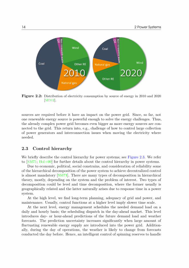
Intermittent renewable energy sources such as solar energy, hydro energy, and windenergy promise to be a feasible solution to the global energy challenge. These energysources are clean compared to fossil fuel, sustainable, plentiful, and the resourcesare available over widely geographical areas, in contrast to fossil fuel there are con-centrated in few countries. Additionally, the energy payback is small meaning theyall ”produce” more energy than they ”consume” [Wei+13; San]. The government inDenmark has established an ambitious and politically broad green energy agreementto point towards the goal of full conversion to renewable energy in 2050. One initia-tive is to increase the share of wind power to 50% of the electricity consumption by2020 as depicted in Figure 2.2 [MD12]. In 2014, a major step towards meeting thesegoals were taken, since 39% of the Danish energy consumption were supplied by windturbines [Eneb].
Intermittent renewable energy sources are stochastic in nature and fluctuates in-dependently from demand. This introduce, e.g., undesirable power imbalance andstability issues. To offset the unavoidable imbalance that will appear during real-time operation of the power systems, different opportunities has been researched.Currently, spinning reserve is allocated in advance as a buffer to cover unexpectedshortages of energy supply in real time. That is, determine the production plan suchthat the power system operates at less than its full capacity. Unfortunately, spinningreserve is very expensive to have. Power generators that quickly can cover shortagesare normally embedded with high startup cost and running cost. Furthermore, onecan dissemble that a better production plan may exist if available power plants werepermitted to operate at full capacity. Thus, reducing the need for reserve capacitywill imply a cost reduction. Another way to facilitate the imbalance is by large-scalestorage capabilities. However, [PSH09] indicates that this field needs further researchand development before it become a reality.
Besides the fluctuating energy supply, a large collection of renewable energy
14 2 Power Systems
Figure 2.2: Distribution of electricity consumption by source of energy in 2010 and 2020[MD12].
sources are required before it have an impact on the power grid. Since, so far, notone renewable energy source is powerful enough to solve the energy challenges. Thus,the already complex power grid becomes even bigger as more energy sources are con-nected to the grid. This return into, e.g., challenge of how to control large collectionof power generators and interconnection issues when moving the electricity whereneeded.
2.3 Control hierarchy
We briefly describe the control hierarchy for power systems; see Figure 2.3. We referto [SM71; Hol+09] for further details about the control hierarchy in power systems.
Due to economic, political, social constrains, and consideration of reliability someof the hierarchical decomposition of the power system to achieve decentralized controlis almost mandatory [SM71]. There are many types of decomposition in hierarchicaltheory, mostly, depending on the system and the problem of interest. Two types ofdecomposition could be level and time decomposition, where the former usually isgeographically related and the latter naturally arises due to response time in a powersystem.
At the high level, we find long-term planning, adequacy of grid and power, andmaintenance. Usually, control functions at a higher level imply slower time scale.
At the next level, energy management schedules the needed demand load on adaily and hourly basis; the scheduling dispatch in the day-ahead market. This levelintroduces day- or hour-ahead predictions of the future demand load and weatherforecasts. The prediction uncertainty increases significantly when large amount offluctuating renewable energy supply are introduced into the power grid. Addition-ally, during the day of operations, the weather is likely to change from forecastsconducted the day before. Hence, an intelligent control of spinning reserves to handle

2.4 Electricity market 15
Adequacy ofgrid and powermaintenance
scheduling
UnitCommitment
EconomicModel
PredictiveControl
PowerSystems Grid
Years
Long-termplanning
Days-Hours
EnergyManagement
Minutes
PowerControl
Seconds
PowerManagement
Time
Figure 2.3: Control hierarchy.
the uncertainties are needed [Mor+14]. The UC model is usually used to find thedispatch that satisfy a forecasted demand load at a minimum cost. As we know, thesemodels can result in high computational complexity due to be generally NP-complete.
At the next level, we apply economic MPC to handle the uncertainty and managethe prediction errors of the renewable power supply at a high frequency level, whichcannot be addressed in the UC level because of the optimization solvers executiontime. The economic MPC is applied in a rolling horizon manner, thus, updated andmore reliable forecasts are used. Figure 2.4 illustrates the idea in the two above-mentioned levels. Energy management plan the hourly power production based onday-ahead forecasts of, e.g., wind power production; see Figure 2.4(a). However, theweather is likely to change during the day of operations and the power supply fromrenewable energy sources is unlikely constant within an hour. E.g., a closer look athour 3 may show a wind power production develop as Figure 2.4(b). This variationmay result in imbalance and inefficient power production.
Lastly, the power management levels relates to system stability like stabilizingvoltage and frequency before the electricity is distributed out to the power grid andfinally to the consumers.
2.4 Electricity market
Electricity is a commodity production there can be bought, sold, and traded. Theelectricity market is a market where contracts are made between seller and buyer forthe delivery of power. Nord Pool Spot is the main arena for trading power in theNorthern Europe and Baltic region. Nord Pool Spot facilitate the day-ahead marketand the intraday marked [Enea; Nor; Mor+14]. These two trading categories areinteresting in context of this thesis.

16 2 Power Systems
0 4 8 12 16 20 240
100
200
300
400
500
600
700
800
900
1000
Time [h]
Win
d P
ower
[MW
]
(a) 24-hours wind power production forecast.
0 10 20 30 40 50 60480
490
500
510
520
530
540
550
Time [min]W
ind
Pow
er [M
W]
(b) Wind power production variation at hour 3.
Figure 2.4: The considered wind power production forecasts on the tow levels: days-hourslevel and minute level.
2.4.1 Day-ahead marketThe day-ahead market takes place the day before energy delivery. A buyer estimatesneeded volume of energy to meet demand the following day and the price willing topay for this volume, hour by hour. A seller decides the volume of energy which canbe delivered and at what price, hour by hour. Deadline for submitting bids is 12:00CET. Elspot setting the price, hour by hour, using the supply and demand principlesand closing the deals taking into account the limitations of the power grid. The poweris physically delivered at 00:00 CET according to the contracts agreed. The majorityof the volume handled by Nord Pool Spot is traded on the day-ahead market.
2.4.2 Intraday marketThe intraday market takes place during the day of operation when the day-aheadmarket is closed. Elbas contributes to balance production and consumption in thepower market for Northern Europe. Elbas is a continuous market where tradingtake place every day until one hour before delivery. Prices are set on a first-come,first-served principle; the best prices come first.
This market is progressively relevant as more renewable energy sources such aswind energy and solar energy are integrating into the power grid. These types ofenergy sources are intermittent and stochastic in nature. Therefore, it is a difficulttask to provide accurate predictions of the amount produced prior to the closing ofthe day-ahead market. Hence, imbalances between day-ahead contracts and producedvolume may need to be equalized.

CHAPTER 3Software
In this chapter, we informally present the software used in this thesis.
3.1 IBM® ILOG® CPLEX® Optimization Studio
We model the mathematical UC optimization problems with IBM ILOG CPLEXOptimization Studio V12.6 by IBMr [IBM14]. This software consolidates an Inte-grated Development Environment (IDE) with the Optimization Programming Lan-guage (OPL) and the state-of-the-art ILOG CPLEX and CP Optimizer solution en-gines. The motivation for applying this optimization software product is primarilydue to following two reasons:
• The modeling language OPL provides built-in tools and a syntax that is veryclose to the mathematical formulation. This makes an easier transition from amathematically written model to a model that is solvable by a computer.
• Permit a clearer separation between model and input data. So, with a littleeffort, the same model can be solved with different input data. The softwarefacilities integration of external data sources like databases and spreadsheetsfrom Microsoft Excel by read and write references.
Figure 3.1 illustrates a simplified overview of IBM ILOG CPLEX Optimization Studio.Comprehensive documentation and release notes for V12.6 are available in [IBM14;IBM11].
3.2 Matlab® MathWorks®
The control framework is modeled and implemented in Matlab® release R2014aby MathWorks® [Mat]. Matlab stands for MATrix LABoratory and is a high-levellanguage and interactive environment. Section 6.5 provide a description of the controlframework and a flowchart of the function calls.
For a better integration with the UC optimization problem and the economic MPCproblem, UC is also implemented in Matlab and solved using IBM ILOG CPLEXOptimizer V12.6 Matlab interface. The control framework is implemented to sup-ports three solvers, which easily can be selected by a flag. The solvers are CPLEX

18 3 Software
IBM ILOGOPL Data
Raw Data:Database
Spreadsheet
IBM ILOGOPL Model
Engines:IBM ILOG
CPLEX/ CPOptimizer Solvers
OptimalSolution
View Solution:Database
Spreadsheet
Impo
rt
Solv
e
Expo
rt
Figure 3.1: Simplified illustration of IBM ILOG CPLEX Optimization Studio.
Optimizer V12.6 developed by ILOG IBM Software [IBM14], MOSEK V7.0 devel-oped by MOSEK ApS [MOS14], and Gurobi Optimizer V5.6 developed by GurobiOptimization, Inc [Gur14]. These are commercial solvers; however, for academic usethe solvers can be provided for free.

Part IITheory

CHAPTER 4Unit Commitment
In this chapter, we give an introduction to the UC optimization problem. We describeand formalize mathematically the components of the UC problem in Section 4.2. Sec-tion 4.3 present the UC optimization problem as a MILP problem. Section 4.4 discussimplementation and a syntax comparison between IBM ILOG CPLEX OptimizationStudio and Matlab, and Section 4.5 informally address the complexity of solvingthe UC problem. In Section 4.6, we demonstrate and apply the formulated UC opti-mization problems in the application of two conceptual power systems.
4.1 Introduction
Planning the power production to match demand load and reserve capacity with afinancial and environmental perspective is nontrivial. Conceptually, consider a port-folio of controllable power generating plants. Then, a planning problem is basicallytwofold:
1. determine which power plants are running each time step and
2. determine the production level for the running plants in a cost effective way.
We say that power plants are committed when turned on and decommitted whenturned off. Finding the optimal cost effective power production plan of the committedplants while satisfying various requirements denotes economic dispatch. This planningproblem may be solved by formulating the Unit Commitment (UC) optimizationproblem. As we see, the problem consist of discrete and continuous decisions, thus, thegeneral UC is a Mixed Integer Programming (MIP) problem. The presences of integervariables yields into a computational complex problem there is not straightforwardto solve. In Section 4.5, we address this further.
In the following, we mathematical formulate the UC optimization problem usedin this thesis. It should be noted that other formulation exist, since the problemis very system dependent. Therefore, for further literature and related research onthis topic includes, e.g., [WW12; OAV12; Cas+11; Pad04; NKF09; ZGH10; RG91;MNG14]. Furthermore, we notice that the notation used in UC may be confusedwith the notation used in economic MPC. It is decided to apply same notation as inthe literature in both fields for not to mislead the reader. However, in context, thenotation should not be misunderstood.

22 4 Unit Commitment
4.2 Mathematical problem formulation
In this section, we present verbally and formulate mathematically the affine objectivefunction and the constraints for the UC optimization problem. The discrete part ofthe problem will be formulated with three binary variables. Thus, we formulate abinary mixed integer linear programming problem.
Consider a set I := {1,2, . . . ,I} of power generating plants and a specified time-varying demand over T := {1,2, . . . ,T} time periods defining the planning time hori-zon. The mathematical programming model involves I × T continuous nonnegativereal variables, pi,t ∈ R≥0; and three I × T binary variables: ui,t, yi,t, zi,t ∈ Z2.
4.2.1 Objective functionThe objective cost function is formulated to minimize the total operating power pro-duction cost. The operating cost consists of running cost, startup cost, and shutdowncost.
The running cost is model by fixed and variable cost. The fixed cost is expressedas
aiui,t, (4.1)
where ai is the fixed cost of plant i and ui,t is a binary variable that is equal to oneif plant i is committed during time period t and zero otherwise. The variable cost isexpressed as proportional to the plant power output:
bipi,t, (4.2)
where bi is the variable cost of plant i and pi,t is the nonnegative real variable that isthe power output of plant i during time period i.
The startup and shutdown cost is considered constant. Every time a plant isstarted up, its startup cost is added. Similar, every time a plant is shut down, itsshutdown cost is added. Thus, we obtain
SUiyi,t + SDizi,t, (4.3)
where SUi and SDi are the startup and shutdown cost of plant i, respectively. yi,t isa binary variable that is equal to one if plant i is started up at the beginning of timeperiod i and zero otherwise and zi,t is a binary variable that is equal to one if planti is shut down at the beginning of time period i and zero otherwise.
The function to be minimized is obtained by combining (4.1)–(4.3), thus, theobjective function of the UC problem is
ϕ =∑i∈I
∑t∈T
[aiui,t + bipi,t + SUiyi,t + SDizi,t] . (4.4)

4.2 Mathematical problem formulation 23
4.2.2 ConstraintsSeveral constraints may be placed to the UC problem, as many different requirementscan be given; e.g., individual requirements on power demand, reliability, physicallimits of equipment, power system operating limits, etc. The list presented here is byno means exhaustive; these are the ones being considered and implement in this thesis.To deduce some of the constraints, we use logical equivalences; see Appendix A.2.1.
4.2.2.1 Power demand load balance
The system power demand should be satisfied for each time period:∑i∈I
pi,t ≥ Dt, t ∈ T , (4.5)
where Dt is the power demand in time period t. Power contribution from non-controllable renewable power sources will change the need for producing power fromthe conventional power plants. PWt represent forecasted power production fromrenewable power sources at time period t. Thus, (4.5) i extended to∑
i∈Ipi,t ≥ Dt − PWt, t ∈ T . (4.6)
4.2.2.2 Spinning reserve
In order to ensure reliability in term of enough resources available during the real-time operation of the power system, the system operator allocates reserve capacityto cover unexpected shortages of energy supply in real-time.
The required spinning reserve should be guaranteed to be available by the com-mitted plants: ∑
i∈IPUiui,t ≥ Dt +Rt, t ∈ T . (4.7)
where PUi is the maximum power output generation of plant i and Rt is the requiredspinning reserve at time period t. Like the demand load balance constraint above, weintroduce PWt in the event of contribution from renewable power sources, thus,∑
i∈I
PUiui,t ≥ Dt +Rt − PWt, t ∈ T . (4.8)
4.2.2.3 Power output limitations
The power plants are limited within an operating range, i.e., if a plant is committed,the power output is to be within its minimum and maximum power output generation.This may be expressed as
PLiui,t ≤ pi,t ≤ PUiui,t, i ∈ I, t ∈ T , (4.9)

24 4 Unit Commitment
where PLi and PUi are the minimum and maximum power output generation of planti, respectively. We see, if plant i at time period t is committed, ui,t = 1, the poweroutput, pi,t, is to be within limits, whereas if plant i at time period t is decommitted,ui,t = 0, the preceding constraint forces pi,t = 0.
4.2.2.4 Ramping rate limitations
The power plants ability to increase and decrease to higher and lower power outputfrom time period k to k+1 is limited. The so called ramp rate limits may be expressedby
pi,t − pi,t−1 ≤ RUi, i ∈ I, t ∈ T , (4.10)pi,t−1 − pi,t ≤ RDi, i ∈ I, t ∈ T . (4.11)
For the time period t = 1, pi,0 is given by the initial output power of plant i. RUi
and RDi are the maximum ramp-up and ramp-down limit of plant i, respectively.
4.2.2.5 Startup and shutdown
Any committed plants can be shut down but and not started up, and analogously,any decommitted plants can be started up but not shut down. This can be expressedby logic constraints with startup and shutdown cost term added, respectively:
ui,t − ui,t−1 ≤ yi,t, i ∈ I, t ∈ T , (4.12)ui,t−1 − ui,t ≤ zi,t, i ∈ I, t ∈ T . (4.13)
For the time period t = 1, ui,0 is given by the plants status preceding the first periodof the planning horizon. By considering the possible scenarios, the logic constraints(4.12) and (4.13) gives intuitively sense. E.g., consider the lefthand side of (4.12).The only scenario this yields to one is when ui,t = 1 and ui,t−1 = 0, thus, startupcost should be added to the objective function. The expressions, however, may bederived from logic conditions [RG91]. Consider the startup scenario. Startup costshould be added to the objective function if ui,t = 1 and ui,t−1 = 0. Let PA denotea committed plant i at time t, ¬PB denote a decommitted plant i at time t− 1, andPC = yi,t denote whether startup cost is add, yi,t = 1, or not, yi,t = 0. Then, wehave
PA ∧ ¬PB ⇒ PC
By (A.11), we can remove the implication, thus
¬(PA ∧ ¬PB) ∨ PC .
By applying (A.12) (De Morgan’s theorem), we have
¬PA ∨ PB ∨ PC .

4.2 Mathematical problem formulation 25
With the implication from above and that, e.g., ¬PA = 1−ui,t, the conjunction formcan be translated into its equivalent mathematical linear form:
1− ui,t + ui,t−1 + yi,t ≥ 1 ⇒ui,t − ui,t−1 ≤ 1,
which is equivalent to (4.12). Likewise, (4.13) can be deduced by same approach.
4.2.2.6 Minimum up- and downtime
Due to physical characteristics, power plants may not immediately be able to startupand shutdown and vice versa. Let TUi denote the minimum uptime for plant i, onceit has started up. If yi,t = 1, then ui,t+1 = 1, ui,t+2 = 1, . . . , ui,t+TUi ; thus, we writethe logic expression
yi,t ⇒∧j∈Ui
ui,t+j , (4.14)
where Ui := {1,2, . . . ,TUi}. By (A.11), (4.14) can be rewritten as
¬yi,t ∨ ui,t+j (4.15)
Translating (4.15) conjunction expression into its equivalent mathematical linear formgives the minimum uptime constraint:
1− yi,t + ui,t+j ≥ 1 ⇒ui,t+j ≥ yi,t, j ∈ Ui. (4.16)
Similar, we derive the minimum downtime. Let TDi denote the minimum downtimefor plant i, once it has been shutdown. If zi,t = 1, then ui,t+1 = 0, ui,t+2 = 0, . . . ,ui,t+TDi , which leads to the logic expression
zi,t ⇒∧
j∈Di
¬ui,t+j , (4.17)
where Di := {1,2, . . . ,TDi}. Hence, its equivalent mathematical linear form gives theminimum downtime constraint:
1− zi,t + 1− ui,t+j ≥ 1 ⇒zi,t + ui,t+j ≤ 1, j ∈ Di. (4.18)
4.2.2.7 Restricting carbon dioxide emission
There may be restricting on carbon dioxide emission when generating power. Thismay be expressed as ∑
i∈I
∑t∈T
ECipi,t ≤ EU, (4.19)
where ECi is the CO2 emission rate for plant i and EU denote the maximum CO2
emission allowed.

26 4 Unit Commitment
4.3 The UC optimization problem
In Section 4.2.1, we present the objective cost function which is to be minimizedwhile satisfying the constraints provided in Section 4.2.2. Two formulations of the UCoptimization problem will be considered; see demonstration of the two in Section 4.6.They differ in terms of whether or not including the minimum up- and downtimeconstraints and the restricting carbon dioxide emission constraint. First, we formulatethe UC optimization problem as the following MILP:
minimize ϕ =∑i∈I
∑t∈T
[aiui,t + bipi,t + SUiyi,t + SDizi,t] (4.20a)
subject to∑i∈I
pi,t ≥ Dt − PWt t ∈ T (4.20b)∑i∈I
PUiui,t ≥ Dt +Rt − PWt t ∈ T (4.20c)
PLiui,t ≤ pi,t ≤ PUiui,t i ∈ I, t ∈ T (4.20d)pi,t − pi,t−1 ≤ RUi i ∈ I, t ∈ T (4.20e)pi,t−1 − pi,t ≤ RDi i ∈ I, t ∈ T (4.20f)ui,t − ui,t−1 ≤ yi,t i ∈ I, t ∈ T (4.20g)ui,t−1 − ui,t ≤ zi,t i ∈ I, t ∈ T (4.20h)ui,t, yi,t, zi,t ∈ Z2 (4.20i)pi,t ∈ R≥0 (4.20j)
with I := {1,2, . . . ,I} thermal generating plants and T := {1,2, . . . ,T} time periodsdefining the planning time horizon.
Including the minimum up- and downtime constraints and the carbon dioxideemission restricting yields into the following:
minimize ϕ =∑i∈I
∑t∈T
[aiui,t + bipi,t + SUiyi,t + SDizi,t] (4.21a)
subject to (4.20b) − (4.20h) (4.21b)ui,t+j ≥ yi,t j ∈ Ui (4.21c)zi,t + ui,t+j ≤ 1 j ∈ Di (4.21d)∑i∈I
∑t∈T
ECipi,t ≤ EU (4.21e)
ui,t, yi,t, zi,t ∈ Z2 (4.21f)pi,t ∈ R≥0 (4.21g)
with I := {1,2, . . . ,I} thermal generating plants, T := {1,2, . . . ,T} time periodsdefining the planning time horizon, Ui := {1,2, . . . ,TUi}, and Di := {1,2, . . . ,TDi}.

4.4 Implementation 27
The difficulties for solving the UC optimization problem (4.20) or (4.21) are due tothe presences of binary variables, since the objective function and all the constraintsare linear.
4.4 Implementation
In this section, we show how the UC problem may be implemented in IBMr ILOGr
CPLEXr Optimization Studio V12.6 and in Matlab by MathWorksr. A compar-ison of the two languages is provided. The Matlab version is implemented suchthat CPLEX Matlab interface is used. We present the code for implementing theobjective function (4.4) and power demand load balance constraint (4.6). The fullimplementations are provided in Source Code Booklet Section 1.1 and Section 2.1,respectively.
Listing 4.1: Syntax for IBM ILOG CPLEX Optimization Studio.1 // Objective function2 minimize3 sum(t in T, i in I) (a[i]*u[i,t] + b[i]*p[i,t]4 + SU[i]*y[i,t] + SD[i]*z[i,t]);5 // Constraints6 subject to {78 // Demand load balance9 forall(t in T) {
10 sum(i in I) p[i,t] >= D[t] - PW[t];11 }12 };
Listing 4.2: Syntax for Matlab.1 % Objective function2 coeffpvar = repmat(b,Horizon,1);3 coeffuvar = repmat(a,Horizon,1);4 coeffyvar = repmat(SU,Horizon,1);5 coeffzvar = repmat(SD,Horizon,1);6 cplex.Model.obj = [coeffpvar; coeffuvar; coeffyvar; coeffzvar];78 % Demand load balance9 cplex.Model.A = [kron(eye(Horizon),ones(1,Nunits)) zeros(Horizon,Nvar)];
10 cplex.Model.lhs = D - PW;11 cplex.Model.rhs = Inf(Horizon,1);
Instantly, we see that the Matlab implementation Listing 4.2 is much more complexand not as simple and intuitive as IBM ILOG CPLEX Optimization Studio Listing 4.1.Some of the reasons for this are outlined in the following. We are considering fourtwo-dimensional decision variables. In Matlab, these decision variables are to bestacked into one one-dimensional vector in the following manner
x =[p u y z
]T.

28 4 Unit Commitment
Each two-dimensional decision variable are again stacked like this
p =[p1,1 p2,1 . . . pN,1 p1,2 p2,2 . . . pN,2 . . . pN,M
]T,
where N is the number of power plants and M the number of planning time periods.Furthermore, each row in the system matrix A represent one constraint for one spe-cific plant for one time period and each column in A represent one decision variablefor one specific plant for one time period. Consequently, a lot of bookkeeping areneeded in the Matlab implementation. Comparing this with the modeling languageOPL syntax in Listing 4.1 truly shows its benefits. The syntax is very close to themathematical formulation. It is light and one can literally just write out the equa-tions. OPL syntax provide an easy way to write an optimization problem for whichis solvable by a computer.
4.5 Solution methods
The general UC problem is nontrivial to solve. The UC problem quickly becomesvery complex and extremely difficult to obtain the optimal solution for system withpractical size (large-scale power systems). In fact, the industry is in some situationscompelled to manually stop the optimization software and simply use the currentiterative obtained solution due to limited period of time. Mathematically, UC is anNP-complete MIP problem, which make it impossible to develop an algorithm withpolynomial computation time; i.e., in worst case, the solution time grows exponen-tially with the problem size [AH04; BMM99; GZP03].
To illustrate the complexity, we consider the brute force methods. Let N denotethe number of power plants and M denote the number of planning time periods. Then,the number of combinations to be evaluated each time period is 2N −1. For the totalplanning horizon, the maximum number of possible combinations is (2N −1)M , whichscales badly and quickly return into an enormous number. E.g., consider N = {10,20}power plants each hour over a 24-hour planning horizon, this result in
N = 10, (210 − 1)24 = 1.73 · 1072
N = 20, (220 − 1)24 = 3.12 · 10144.
Thus, the number of combinations immediately becomes very big. Of course, not allcombinations are feasible solutions sets, nevertheless, all need to be checked.
There exist many optimization techniques for solving the UC problem, e.g.,
• Priority list schemes
• Dynamical programming
• Lagrangian relation
• Branch-and-bound method

4.6 Case study 29
Solution methods for UC problems are an important topic; however, a study to coverthem is outside the scope of this thesis. Therefore, for further information of thevarious methods available for solving the UC problem see, e.g., [SK98; WW12].
4.6 Case study
In this section, we establish two conceptual power systems to demonstrate the formu-lated UC optimization problem. Firstly, we apply (4.20) to a 3-unit power system.Secondly, we apply (4.21) to a complex 10-unit power system. Besides complexity,they differ in terms of specific system requirements. Renewable power contributionis fixed to zero: PWt = 0, ∀t.
The case studies are implemented in IBM ILOG CPLEX Optimization Studiousing CPLEX 12.6 and are provided in Source Code Booklet Chapter 1. [Cas+11;ZGH10] inspired the two case studies.
4.6.1 3-unit power systemWe consider three power plants over a three hour planning horizon. Table 4.1 lists thedemand load to be satisfied for each time period and Table 4.2 lists the operationalparameters of the power plants. Let all plants be decommitted at time period t = 0.
The UC optimization problem (4.20) presented mathematically in Section 4.3 issolved for global optimality. The MILP problem for the 3-unit system contains 60constraints and 37 variables, where 27 are binary variables. The obtained optimalpower production plan, reported in Table 4.3, result in a minimum cost of $191.
We see that the demand load, the spinning reserve, and the system requirementsare satisfied. Even though this case study is small a trend can be deduced. Theheavier generators are scheduled first (close to their maximum capacity), while the
Table 4.1: 3-hour demand load for the 3-unit power system [MW].
Hour Dt Rt
1 150 152 500 503 400 40
Table 4.2: Operational parameters for the 3-unit power system.
Unit ai bi SUi SDi PLi PUi RDi RUi
[$/h] [$/MWh] [$/h] [$/h] [MW] [MW] [MW/h] [MW/h]1 5 .100 20 5 50 350 300 2002 7 .125 18 3 80 200 150 1003 6 .150 5 1 40 140 100 100

30 4 Unit Commitment
Table 4.3: Optimal production plan for the 3-unit power system [MW].
Plant Hour1 2 3
1 150 350 3202 0 100 803 0 50 0
4 8 12 16 20 24600
800
1000
1200
1400
1600
1800
Tot
al P
ower
[MW
]
Time [h]
Demand load Spinning reserves
Figure 4.4: 24-hour demand load for the 10-unit power system [MW].
smaller generators are used to deal with the fluctuations in the demand load. Thiscorresponds to a commonly used scheduling strategy called Priority List (PL) scheme[SK98; WW12].
4.6.2 10-unit power systemWe consider ten power plants over a 24-hour planning horizon. Figure 4.4 representsthe demand load to be satisfied for each time period; see Appendix B Table B.1(a) fornumerical representation. The spinning reserve is set as a 10% of the demand load foreach time period. The power plants operational parameters are listed in Appendix BTable B.2. Let all plants be decommitted at time period t = 0 and let the maximumCO2 emission be fixed to 15,500 g.
The UC optimization problem (4.21) presented mathematically in Section 4.3 issolved for global optimality. The MILP problem contains 7,335 constraints and 961variables, where 720 are binary variables. The obtained optimal power productionplan, reported in Figure 4.5, result in a minimum cost of $572,395. Figure 4.6 illus-trates the optimal power production plan for plant 1.
In the following, we show that the obtained solution complies with the system re-quirements. Figure 4.7 shows that the obtained production plan satisfy the demandload (production exactly equals the demand load) and the spinning reserve require-

4.6 Case study 31
Time (h)
Pow
er P
rodu
ctio
n [M
W]
5 10 15 200
100
200
300
400
500Plant 1
5 10 15 20150
200
250
300
350
400
450
500Plant 2
5 10 15 20
20
40
60
80
100
120
140Plant 3
5 10 15 20
20
40
60
80
100
120
140Plant 4
5 10 15 2020
40
60
80
100
120
140
160
Plant 5
5 10 15 20
0
20
40
60
80
Plant 6
5 10 15 20
0
20
40
60
80
Plant 7
5 10 15 20
0
10
20
30
40
50
60Plant 8
5 10 15 20
0
10
20
30
40
50
60Plant 9
5 10 15 20
0
20
40
60Plant 10
Figure 4.5: The optimal power production plan for each plants (blue line) with each plantsminimum and maximum power output (red dashed line).
ment at each time period. Figure 4.5 and Figure 4.8 show that the plants minimumand maximum power output and ramping limits are fulfilled at each time period, re-spectively. Lastly, the CO2 emission is exactly below the maximum. Consequently,the formulated constraints (4.21) are satisfied.
Figure 4.9 and Figure 4.10 illustrates the distribution of the four cost compo-nents in the objective function. The total production cost dominates by the variablecost accounting for ∼82% of the total production cost. Next is the fixed cost with∼18%, while startup and shutdown only account for <1%. Consequently, the totalproduction cost follows more or less the demand load.

32 4 Unit Commitment
4 8 12 16 20 240
100
200
300
400
500
Pla
nt #
1 [M
W]
Time [h]
Power production PL/PU
Figure 4.6: The optimal power production plan for plant 1 with its minimum and maxi-mum power output limits.
4 8 12 16 20 24500
1000
1500
2000
Tot
al P
ower
[MW
]
Time [h]
Figure 4.7: The total production plan (dotted yellow) satisfy demand load (solid blue);coincide throughout planning horizon. The actual spinning reserve (dottedcyan) obey the required spinning reserve (dotted red).

4.6 Case study 33
Time Step
Pow
er O
utpu
t Cha
nge
(Ram
ping
)
5 101520−200
−100
0
100
200Plant 1
5 101520−200
−100
0
100
200Plant 2
5 101520−100
−50
0
50
100
Plant 3
5 101520−100
−50
0
50
100
Plant 4
5 101520−100
−50
0
50
100
Plant 5
5 101520−50
0
50
Plant 6
5 101520−50
0
50
Plant 7
5 101520−50
0
50
Plant 8
5 101520−50
0
50
Plant 9
5 101520−50
0
50
Plant 10
Figure 4.8: Change in power output for each time step (solid blue) with each plant ramp-ing limits (dotted red).
4 8 12 16 20 240
1
2
3
4x 10
4
Pro
duct
ion
Cos
t [$]
Time [h]
Figure 4.9: The total production cost (solid black) over the planning horizon. The vari-able cost (dotted blue), the fixed cost (dotted red), and startup and shutdowncost (dotted cyan).

34 4 Unit Commitment
Variable cost: 82%
Fixed cost: 18%
Startup and shutdown cost: < 1%
Figure 4.10: Distribution of the four cost components in the objective function.

4.7 Summary 35
4.7 Summary
This chapter formulates mathematically the UC optimization problem as a MILPproblem. We show that the OPL syntax provided in IBM ILOG CPLEX Optimiza-tion Studio is very close to the mathematical formulation compared to the Matlabsyntax and informally present optimization techniques for solving the UC problem.Lastly, we apply the formulated UC optimization problems at two conceptual powersystems. The case studies demonstrate the UC and that the implementation behavesas expected.

36

CHAPTER 5Models for Predictive
ControlThis chapter present key parts in development of our economic MPC framework inChapter 6. We outline the basic idea of modeling dynamical systems for predictivecontrol. In Section 5.2, we formulate the mathematical model applied for modelingthe dynamics of a power system (portfolio of power generating plants). Section 5.3define a finite impulse response model and Section 5.4 present a Kalman filtering andprediction for the linear time-invariant discrete-time state-space models formulatedin Section 5.2. Additionally, in the presence of unmeasured nonzero disturbance,Section 5.5 present how to achieve offset free tracking performance for MPC.
5.1 Modeling dynamical systems
A dynamical system describes the behavior of a physical system evolution over time.The variables describing the state of the mathematical system, at any given time, arecharacterized by its state variables. The state variables are stacked in a time-varyingstate vector x(t), t ∈ R. The set of all the possible values of the state variables is thestate-space. As the process evolve in time, the state variables change from its initialstate x(t0) = x0 by the underlying dynamical processes. A dynamical system may,e.g., be modeled by systems of ordinary differential equations in the form
d
dxx(t) = x(t) = f(x(t), u(t), d(t), w(t)), x(t0) = x0, (5.1)
where x(t) is the state vector, u(t) is the manipulated input variables, d(t) is thedisturbance, and w(t) is the stochastic process noise. The measured outputs, y(t),and the controlled outputs, z(t), may be modeled by
y(t) = g(x(t), v(t)) (5.2a)z(t) = h(x(t)), (5.2b)
where v(t) is the stochastic measurement noise. The deterministic formulation isobtained without measurement and process noise. Let nx denote the number ofcoupled nonlinear differential equations, which also is the number of variables in x.

38 5 Models for Predictive Control
Process
vw
u
d
y
z
Figure 5.1: A generic stochastic input-output model.
State-SpaceModel
ARX StepResponse
ImpulseResponse
ARMAX SDE
Box-Jenkins Kalman Filterand Predictor
TransferFunction
Figure 5.2: State-space model realization of linear time-invariant models.
Following that notation, we label x ∈ Rnx , u ∈ Rnu , y ∈ Rny , and z ∈ Rnz . In thisthesis, linear systems of finite dimension will be considered, thus, the functions f , g,and h are linear.
The generic input-output model relations consist of a process model of the system(5.1), the sensor function (5.2a), and the output function (5.2b). The block diagramin Figure 5.1 illustrates the above stochastic formulation.
There exist several methods for achieving mathematical models in which describea dynamical system. Many time-invariant mathematical models can be formulatedas a discrete-time state-space model as depicted in Figure 5.2. This formulation isbeneficial in the control framework presented in Chapter 6. Each of the realizationmodels depicted in Figure 5.2 will not be addressed, since it would be outside the scopeof the thesis. Appendix A.1 provide background material of the basic concepts of howa linear time-invariant continuous-time model may be linearized and discretized toobtain a linear time-invariant discrete-time state-space model, for which is suitablefor control problems. For further literature to this subject, consult, e.g., [Jør11; Jør05;Mac02; Hal+14; Dat04].

5.2 Modeling power systems 39
5.2 Modeling power systems
In this section, we present the system models applied for modeling a power system. Weformulate both a MIMO system and a MISO system. We consider a linear distributedsystem with independent power generators there must satisfy their own objectivewhile collaborate to satisfy a common objective, the overall demand load.
5.2.1 Power system dynamicsThe power system consists of a portfolio of nu controllable power generators (e.g.thermal power plants) and a portfolio of nd non-controllable predictable power gen-erators representing the power production from the renewable energy sources. Weassume that the non-controllable power generators are farms of wind turbines.
Each individual power generators are independent systems and modeled separately,as the activity in one generator does not directly affect the others. However, theyare coupled in order to collaborate to satisfy the overall power demand load. Werepresent the controllable and non-controllable power generators by following linearsystems
Zu,i(s) = Gi(s)Ui(s), i= 1,2, . . . ,nu, (5.3a)Zd,j(s) = Dj(s), j= 1,2, . . . ,nd. (5.3b)
Ui(s) is the manipulable variables describing the unit of fuel supplied to plant i, Dj(s)is the known forecast from wind turbine j, Zu,i(s) is the power produced by plant i,and Zd,j(s) is the power produced by wind turbine j. The transfer functions Gi(s)describe system dynamics for plant i. The total power production is obtained by
ZT (s) =
nu∑i=1
Zu,i(s) +
nd∑j=1
Zd,j(s)
=
nu∑i=1
Gi(s)Ui(s) +
nd∑j=1
Dj(s).
(5.4)
We model the dynamics of the controllable power plants, Gi(s), with following thirdorder model
Gi(s) =1
(τis+ 1)3. (5.5)
This third order model has been provided and validated against experimental data atDONG Energy, Denmark [EMB09]. Let the non-controllable power generators be awind turbine. The dynamics of a wind turbine may be model by following first ordermodel [EMB09; Hov13]
Hj(s) =1
τjs+ 1, (5.6)
with a time constant, τj , less than 5 seconds. Wind turbines have fast dynamicsand react very quickly to set-point changes. In fact, the dynamics will be drowned

40 5 Models for Predictive Control
Am
plitu
de
0 20 40 60 80 100 120 140 160 180 2000
0.5
1
Time [s]
Wind, τ = 5
0 20 40 60 80 100 120 140 160 180 2000
0.5
1
Plant, τ = 10
0 50 100 150 200 2500
0.5
1
Plant, τ = 20
Figure 5.3: Deterministic step responses of the transfer functions (5.5) and (5.6) dis-cretized using zero-order hold with sampling time of Ts = 20 seconds.
by the power plant dynamics and discretization, and thereby have no influence inour simulations. Therefore, we disregard the first order transfer function and replaceHj(s) = 1 ∀j. The forecasted power production from the renewable energy sourcesare assumed to be in power [MW]. If the controller would get, e.g., the wind speed ofwind turbines one could incorporate this into the model.
5.2.1.1 Step response
We perform a deterministic step response of the two transfer functions (5.5) and (5.6)in discrete-time with time constants τ = {20, 10} and τ = 5, respectively. Figure 5.3illustrates the system reaction on a step.
For the power plant systems, we obtain an instantly positive response and a gainK = 1. These observations are consistent with the given transfer functions (5.5). Asexpected, the dynamic of the wind turbine is drowned, which verify our assumptionabove. We see that sampling time of Ts = 20 seconds is adequate enough to capturethe system dynamics while not been too detailed. Hence, this sampling time or lowerwill be used throughout the economic MPC simulations.

5.2 Modeling power systems 41
5.2.2 Discrete-time state-space model formulationThe stochastic linear system in continuous-time used to describe the dynamics of thepower system (see Section 5.2.1) is represented as
Z(s) = G(s) (U(s) +W (s)) +H(s)D(s) (5.7a)= G(s) (U(s) +W (s)) +D(s) (5.7b)
with the measurementsY (s) = Z(s) + V (s). (5.8)
U(s) is the manipulable variables, D(s) is the known forecast, W (s) is stochasticprocess noise, V (s) is stochastic measurement noise, Z(s) is the output, and Y (s) isthe measurements. The deterministic linear system in continuous-time is obtainedwith W (s) = V (s) = 0, i.e.,
Z(s) = G(s)U(s) +D(s) (5.9a)Y (s) = Z(s). (5.9b)
G(s) and H(s) are transfer function matrices of compatible size in order to obtain thedesired system. Cf. Section 5.2.1, H(s) = 1. Using a zero-order hold discretizationof the continuous-time variables, assumed to be piecewise constant, (5.7) and (5.8)may be represented as the stochastic discrete-time state-space model
xk+1 = Axk +Buk +Gwk (5.10a)yk = Cxk + dk + vk (5.10b)zk = Czxk + dk, (5.10c)
where k ∈ N0 := {0,1, . . . ,N}, with N being the predictive horizon, and G = B.Assume that the model and the true system are identical. Then, the uncertainties inthe state prediction arise from the stochastic process noise and measurement noise.Hence, the optimal filter and predictor is the Kalman filter and predictor [Hal+14].We presented the Kalman filtering and prediction in Section 5.4.
By similar approach, (5.9) may be represented as the deterministic discrete-timestate-space model
xk+1 = Axk +Buk +Gwk (5.11a)yk = Cxk + dk (5.11b)zk = Czxk + dk, (5.11c)
with k ∈ N0. In our simulations, we apply both (5.10) and (5.11).

42 5 Models for Predictive Control
5.2.3 Distributed independent power system
We consider a distributed independent system. The dynamically independently powergenerators must satisfy their own objective while collaborate to satisfy a common ob-jective, the overall demand load. To obtain these properties, we formulate a Multiple-Input and Multiple-Output (MIMO) system. A special case of the MIMO system,the Multiple-Input and Single-Output (MISO) system, is also formulated for the pur-pose of only satisfying the overall demand load. Both formulations are used in oursimulations. In the following, we present the MIMO system the MISO system in thatorder.
Applying (5.3) and (5.4). Then, this representation may be related to (5.9) by
Z(s) =[Zu,1(s) Zu,2(s) · · · Zu,nu(s) ZT (s)
]TU(s) =
[U1(s) U2(s) · · · Unu(s)
]TD(s) = Zd,1(s) + Zd,2(s) + · · ·+ Zd,nd
(s).
The transfer function G(s) is represented as
G1(s)
G2(s). . .
Gnu(s)
G1(s) G2(s) · · · Gnu(s)
.
Let xi,k denote the states variables for plant i, ui,k denote the manipulable variablefor plant i, dj,k denote the know forecast for wind turbine j, zi,k denote power outputfor plant i, and zT,k denote the total power output. Then, (5.11) may be stated bythe block-angular structure
x1,k+1
x2,k+1
...xnu,k+1
=
A1
A2
. . .Anu
x1,k
x2,k
...xnu,k
+
B1
B2
. . .Bnu
u1,k
u2,k
...unu,k

5.3 Finite impulse response 43
z1,kz2,k
...znu,k
zT,k
=
C1
C2
. . .Cnu
C1 C2 · · · Cnu
x1,k
x2,k
...xnu,k
+
0...0
d1,k + d2,k + · · ·+ dnd,k
.
The known forecast, D(s), only have effect on the total power output.We present the MISO system by consider a power system with two power plants,
nu = 2, and a wind farm, nd = 1; see Figure 5.4. Above assumptions are still valid.The total power production is given by
ZT (s) = G1(s)U1(s) +G2(s)U2(s) +D1(s). (5.12)
The first two terms are the output from plant 1, Z1(s), and plant 2, Z2(s), while thelast term is the output from wind farm, Z3(s). We represent Z1(s) and Z2(s) as thediscrete-time state-space model
Zi(s) = Gi(s)Ui(s) ⇒
xi,k+1 = Aixi,k +Biui,k
zi,k = Cixi,k,i = 1,2. (5.13)
The discrete-time state-space model for Z3(s):
Z3(s) = D1(s) ⇒{z3,k = dk. (5.14)
Rewriting into matrix form yields[x1,k+1
x2,k+1
]=
[A1 0
0 A2
][x1,k
x2,k
]+
[B1 0
0 B2
][u1,k
u2,k
](5.15a)
zk = z1,k + z2,k + z3,k =[C1 C2
] [x1,k
x2,k
]+ dk. (5.15b)
5.3 Finite impulse response
We introduce a Finite Impulse Response (FIR) model for representation of dynamicsfor the discrete-time state-space model (5.11) [PJ08; ESJ09]. This is possible forstable processes. Given the current state, we can predict the expected future stateevolution by combining (5.11a)–(5.11c). The state, xk, may be represented in termsof the initial state, x0, and the past inputs, {ui}k−1
i=0 ,
xk = Akx0 +
k−1∑i=0
Ak−1−iBui. (5.16)

44 5 Models for Predictive Control
Plant 1Z1(s) = G1(s)U1(s)
Plant 2Z2(s) = G2(s)U2(s)
Wind FarmZ3(s) = D1(s)
Load (MW)
z1 z2 z3
z
u1 u2 d
MPC
Figure 5.4: Power grid with two controllable conventional power plants and one non-controllable predictable power generator, farms of wind turbines.
This expression for the states, the measured output, yk, and the control output zk,may be related to the initial state, x0, and the past inputs, {ui}k−1
i=0 , by
yk = Cxk + dk
= C
(Akx0 +
k−1∑i=0
Ak−1−iBui
)+ dk
= CAkx0 +k−1∑i=0
CAk−1−iBui + dk
= CAkx0 +
k−1∑i=0
Hyu,k−iui + dk, (5.17)
zk = Czxk + dk
= CzAkx0 +
k−1∑i=0
Hzu,k−iui + dk, (5.18)

5.4 Kalman filtering and prediction 45
with k = 1,2, . . . ,N and the impulse response coefficient (Markov parameters) definedby
Hyu,i = CAi−1B, i = 1,2, . . . ,N, (5.19a)
Hzu,i = CzA
i−1B, i = 1,2, . . . ,N. (5.19b)
N is the number of approximate time steps needed to represent the impulse response.The impulse response coefficients may be obtained by observing the output afterapplying a pulse input vector; i.e., let u0 = 0 and uk = 0 ∀k > 0.
The dynamics in (5.17) and (5.18) can be represented by the linear relation[ESJ09],
Y = Φyx0 + ΓyuU +D
Z = Φzx0 + ΓzuU +D,
where we define the vectors,
Y =
y1
y2...yN
, Z =
z1
z2...zN
, U =
u0
u1
...uN−1
, D =
d1
d2...
dN
,
and the matrices
Φy =
CA
CA2
...CAN−1
, Φz =
CzA
CzA2
...CzA
N−1
, Γu =
Hβ
u,1 0 . . . 0
Hβu,2 Hβ
u,1 . . . 0...
... . . . ...Hβ
u,N Hβu,N−1 . . . Hβ
u,1
,
with β ∈ {y,z}.
5.4 Kalman filtering and prediction
We develop the filter and predictor for the stochastic linear time-invariant discrete-time system (5.10) with process noise, wk, and measurements noise, vk, assumed tobe identically independently normally distributed (iid) as[
wk
vk
]∼ Niid
( [0
0
],
[Rww Rwv
Rvw Rvv
] ). (5.20)
Let the process noise, wk, and the measurement noise, vk, be correlated, i.e., Rwv =RT
vw = 0. Let the initial state, x0 ∼ N(x0|−1,P0|−1), be independent of {wk} and {vk}.

46 5 Models for Predictive Control
We assume that the system is stochastic stationary, i.e., P0|−1 = P . P is computedby the solution of the discrete algebraic Riccati equation (DARE) [JHR11]:
P = APAT +GRwwGT
− (APCT +GRwv)(Rvv + CPCT )−1(APCT +GRwv)T .
In case of above assumption is not valid, one can easily obtain the recursive Kalmanfilter by letting the Kalman filter gain and covariance matrix, P , be time depen-dent. Consequently, be calculated in each time step. Our implementation offers thisopportunity too.
According to the theory of linear estimation [KSH00; JHR11; Sta+12], the optimalpredictor of a system governed by (5.10) is based on the past measurements, {yj}kj=0,and past control inputs, {uj}k−1
j=0 . The filter estimator for the measurement update isslightly different than the standard Kalman filter due to the introduction of dk. Givena new measurement, yk, and the conditional prediction of the disturbance, dk|k−1, theoptimal filtered state estimate, xk|k, is obtained by first computing the innovation
yk|k−1 = Cxk|k−1 + dk|k−1 (5.21a)ek = yk − yk|k−1 (5.21b)
and subsequently compute the innovation covariance and the Kalman filter gain ma-trices used by the filter and the one-step-ahead predictor by
Rfe = CPCT +Rvv (5.22a)Kfx = PCTR−1
fe (5.22b)Kfw = RwvR
−1fe . (5.22c)
The current filtered state estimate, xk|k, and process noise estimate, wk|k, are obtainedby
xk|k = xk|k−1 +Kfxek (5.23a)wk|k = Kfwek. (5.23b)
The one-step-ahead prediction of the states, xk+1|k, the (j+1)-step-ahead predictionsof the states, xk+1+j|k, as well as the output are obtained by
xk+1|k = Axk|k +Buk|k +Gwk|k (5.24a)xk+1+j|k = Axk+j|k +Buk+j|k, j = 1,2, . . . ,N − 1 (5.24b)zk+j+1|k = Czxk+1+j|k + dk+j|k, j = 0,1, . . . ,N − 1 (5.24c)
where N is the predictive horizon and ∀k ≥ 0. In case of uncorrelated process andmeasurement noise, Rwv = RT
vw = 0. Then, Kfw = 0 implying wk|k = 0, thus, theterm Kwk|k is zero and drops out.

5.5 Disturbance modeling for offset-free MPC 47
5.5 Disturbance modeling for offset-free MPC
In closed-loop systems, the controller using the linear process model (5.10) describedin Section 5.2.2 may never reach the desire control trajectory if unmeasured nonzerodisturbances enters the system or if model error is present. To achieve offset freetracking performance for MPC, in the presence of unmeasured nonzero disturbance,the traditional approach is to incorporating disturbance states into the process model.Thus, designs a control system for which can remove asymptotically constant, nonzerodisturbances [Huu+10; MB02].
Let pk ∈ Rnp denote the unmeasured disturbance, np is the number of augmentedoutput disturbance states. Introduce pk into (5.10) yields
xk+1 = Axk +Buk +Bppk +Gwk
yk = Cxk + Cppk + dk + vk.
Assume that the disturbance evolves aspk+1 = pk + ξk
and that the noise in the system is distributed as wk
ξk
vk
∼ Niid
0
0
0
,
Rww 0 Rwv
0 Rξ 0
Rvw 0 Rvv
.
Then, we construct an output disturbance model using the following augmented state-space model[
xk+1
pk+1
]=
[A Bp
0 I
][xk
pk
]+
[B
0
]uk +
[G 0
0 I
][wk
ξk
](5.25a)
yk =[C Cp
] [xk
pk
]+ dk + vk. (5.25b)
Let Bd = 0 and Cd = I and we obtain the output disturbance model.We present the modification for the Kalman filtering and prediction when applying
the disturbance model. The output disturbance is estimated using the augmentedstate-space model (5.25). Now, the one-step-ahead prediction equations are definedas
xk+1|k = Axk|k +Buk|k +Gwk|k
pk+1|k = pk|k.
The innovation is computed as
yk|k−1 =[C Cp
] [ xk|k−1
pk|k−1
]+ dk|k−1 (5.26a)
ek = yk − yk|k−1. (5.26b)

48 5 Models for Predictive Control
The optimal filtered state estimates and process noise estimates are obtained by[xk|k
pk|k
]=
[xk|k−1
pk|k−1
]+
[Kfx
Kfp
]ek (5.27a)
wk|k = Kfwek. (5.27b)
By an appropriate design of the Kalman filter gain matrices Kfx, Kfp, and Kfx.Consequently, the stationary Kalman filter are represented by (5.26) and (5.27). Thestate estimator can estimate the unmeasured nonzero disturbance and render thecontroller capable of offset free MPC.
5.6 Summary
This chapter present key parts in models for predictive control. We formulate themathematical model applied for modeling the dynamics of a power system (portfo-lio of power generating plants). We define finite impulse response model present aKalman filtering and prediction for the linear time-invariant discrete-time state-spacemodel. In addition, we extend the model to achieve offset free MPC in the presenceof unmeasured nonzero disturbance.

CHAPTER 6Economic Model
Predictive ControlThis chapter motivates the choice of economic MPC. We formulate a soft constrainedlinear economic MPC problem and show how it can be formulated as a LP problem.The finite impulse response model and the Kalman filtering and prediction defined inChapter 5 will be used. Section 6.3 provides the controller algorithm and Section 6.5present the developed Matlab implementation. In Section 6.6, we demonstrate andapply the formulated and implemented control framework to a power system.
6.1 Introduction
Model Predictive Control (MPC) is a control methodology for optimal operationand control of dynamical systems and processes [Jør05; Mac02; PJ08; QB03; CM87;Hal+14; Hov13]. In the process industries like chemical plants and oil refineries,MPC has been very popular due to its natural and explicit handling of multivariableconstrained optimal control problems. Besides the feature of incorporating constraintsin the controller, MPC has the capability to integrate predictions and forecasts of theconsidered system. I.e., MPC can anticipate future events and can take control actionsaccordingly, which, e.g., PID controller do not support.
MPC computes an optimal action based on a dynamical system, which may be aempirical model obtained by system identification, and its predicted future evolution.The objective may be related to forcing the system to follow a predefined trajectory orrelated to a cost function, e.g., maximizing profit or minimizing costs. An advantageof MPC is the fact that it is mathematically formulated as a real-time optimizationproblem that repeatedly computes the control actions. That is, for each time step afinite time horizon optimization problem is solved. The optimization yields an optimalinput sequence for the entire horizon, in which only the inputs associated with thattime step are implemented in the physical plant [Mac02]. New measurements areobtained from the physical plant and the real-time optimization approach repeats.This principle is referred to as receding horizon control and is depicted in Figure 6.1.By repeating this optimization scheme, we obtain closed-loop feedback. This allowthe possibly to react to model uncertainties and external disturbances.

50 6 Economic Model Predictive Control
...
Figure 6.1: Control principle of MPC scheme - moving horizon estimation [Wik].
Regulator
Estimator
Plant
Sensor
x
ru z
y
MPC
Figure 6.2: A MPC system [PJ08].
Figure 6.2 illustrates a general control system. A MPC system consists of anestimator and a regulator. Inputs to the MPC is the target trajectory, r, and the esti-mated state, x, that may be obtained by a Kalman filter using historical data. Then,MPC return manipulated inputs, u, to the physical plant, such that the predictedoutput, z, obey the target as well as possible. The aim in our work is to minimizethe operating costs associated with operation of power systems rather than tracking apredefined trajectory as in the traditional MPC framework. Economic MPC providesa MPC framework that minimizes the cost of operations subject to constraints.
We notice that the notation used in UC may be confused with the notation usedin economic MPC. It is decided to apply same notation as in the literature in bothfields for not to mislead the reader. However, in context, the notation should not bemisunderstood.

6.2 Mathematical problem formulation 51
6.2 Mathematical problem formulation
We formulate a soft constrained economic MPC optimization problem. The objectiveof the economic MPC is to implement a feedback strategy, such that the systemremains feasible while the production cost
ϕ =N−1∑k=0
(cTk uk + ρTk+1sk+1
)+ ∥∆uk∥1,αk
, (6.1)
over the control and prediction horizon, N , is minimized. The objective cost function(6.1) is linear in uk and sk+1. In the following, an interpretation of (6.1) is given inthe setting of considering one power plant.
The term, cTk uk, define the cost of producing power, i.e., the cost of fuel, taxes,emission, etc. ck is the cost vector there may be time-varying and uk is the computedcontrol inputs. The manipulable inputs are subject to input constraints; the allowableoperating range and the rate of movement, respectively,
uk ≤ uk ≤ uk (6.2a)∆uk ≤ ∆uk ≤ ∆uk, (6.2b)
where uk and uk is the minimum and maximum value of the manipulable inputvariable, respectively. ∆uk and ∆uk is the maximum rate of movement (ramp-downand ramp-up), respectively, with ∆uk = uk − uk−1.
The system output, zk, are limited to be within the interval
zk ≤ zk ≤ zk,
where zk and zk is the minimum and maximum power output. The interval mayrepresent the overall demand load or the production plan for the individual powerplant provided by solving the UC problem. For some scenarios, it may be impossible orvery expensive to meet the output constraints, which leads to infeasible optimizationproblems with no solution. Therefore, to ensure feasible production plan {uk}Nk=0,we soften the hard output constraints by introducing the slack variable sk, sk ≥ 0,[ZJM10]. Thus,
zk − sk ≤ zk ≤ zk + sk.
The slack variable is minimized and penalized with the weight ρk+1, hence, the term,ρTk+1sk+1. This penalty can be interpreted as, e.g., the price for selling to othersor buying elsewhere to meet the demand load. The penalty is modeled such thatone can penalize individually on the power plants as well as the total production.Furthermore, the penalty is selected sufficiently large such that demand load is metwhenever possible; i.e., s is only nonzero if the output is not within the interval.
The last term, ∥∆uk∥1,αk, discourages disproportionate movement of the manip-
ulable variables by penalizes excessive movement of the input with weight αk. Thisregularization term is important to obtain a realistic well behaved control action andhelps reduce wear and tear of the systems.

52 6 Economic Model Predictive Control
6.3 The economic MPC formulation
In Section 5.2, we defined a stochastic linear time-invariant discrete-time state-spacemodel (5.10) and in Section 5.4 established the optimal filtering and prediction for thissystem. We formulate the finite horizon soft constrained linear regulation problemand describe the economic MPC controller algorithm for computing the manipulatedvariables, uk, for this system [Sta+12; Hal+14]. Algorithm 1 lists the economic MPCcontroller algorithm.
At any time step k, we solve a finite horizon open-loop optimal control problem bylooking N prediction steps ahead and using the current state as the initial state. Thefirst control input from the optimal control sequence, obtained by the optimization,is applied to the plant. We define the power production range, Rk, and the forecastof power supply from renewable energy sources, Dk, as
Rk ={zk+j+1|k, zk+j+1|k
}N−1
j=0, (6.3a)
Dk ={dk+j|k
}N−1
j=0. (6.3b)
We define the objective cost function
ϕ =∑j∈N0
(cTk+j|kuk+j|k + ρTk+j+1|ksk+j+1|k
)+∥∥∆uk+j|k
∥∥1,αk+j|k
.
The optimal trajectory of the predicted manipulated variables and slack variables,{uk+j|k, sk+j+1|k
}N−1
j=0, are obtained by the solution to the soft constrained linear
economic MPC optimization problem
minimize{u,s}
ϕ({uk+j|k,sk+j+1|k
}N−1
j=0) (6.4a)
subject to xk+1|k = Axk|k +Buk|k +Gwk|k (6.4b)xk+1+j|k = Axk+j|k +Buk+j|k j ∈ N1 (6.4c)yk+j+1|k = Cxk+1+j|k + dk+j|k j ∈ N0 (6.4d)zk+j+1|k = Czxk+1+j|k + dk+j|k j ∈ N0 (6.4e)uk+j+1|k ≤ uk+j|k ≤ uk+j+1|k j ∈ N0 (6.4f)∆uk+j+1|k ≤ ∆uk+j|k ≤ ∆uk+j+1|k j ∈ N0 (6.4g)zk+j+1|k + sk+j+1|k ≥ zk+j+1|k j ∈ N0 (6.4h)zk+j+1|k − sk+j+1|k ≤ zk+j+1|k j ∈ N0 (6.4i)sk+j+1|k ≥ 0 j ∈ N0 (6.4j)
where j ∈ Ni := {0 + i,1 + i, . . . ,N − 1}, with N being the predictive horizon. Byincluding the possible non-zero filtered process noise, wk|k, in (6.4b), the regulator

6.3 The economic MPC formulation 53
allows for possible cross-couple process and measurement noise in the stochastic linearstate-space model describing the system.
The function that solves (6.4) and select uk|k is denoted as
uk|k = uk|k = µ(xk|k, uk−1,Rk,Dk). (6.5)
Hence, at time step k we compute, based on looking N time step ahead, the optimalsequences
{uk|k
}N−1
k=0in which the predicted output trajectory, {zk}N−1
k=0 , obey theallowable power production range. Then, the first input, uk|k, from
{uk|k
}N−1
k=0is ap-
plied. This recur in a receding horizon manner as new information becomes available[JHR11].
6.3.1 StabilityStability of economic MPC framework is a very important theme, which certainty hasits attention in the literature [AAR12; Raw+08; May+00]. In this thesis, however,we do not focus on stability issue. Instead we are aware of choosing sufficient longprediction and control horizon compared to system dynamics, and to apply linearstable systems to obtain stability properties according to [May+00].

54 6 Economic Model Predictive Control
Algorithm 1 Economic MPC with external forecastsRequire yk, uk−1, xk−1|k−1, the external forecasts
Rk ={zk+j+1|k, zk+j+1|k
}N−1
j=0
Dk ={dk+j|k
}N−1
j=0,
and the Kalman filter gain matrices
Rfe = CPCT +Rvv
Kfx = PCTR−1fe
Kfw = RwvR−1fe
Compute one-step-ahead predictorCompute the one-step-ahead predictor
xk|k−1 = Axk−1|k−1 +Buk−1 +Gwk−1|k−1
yk|k−1 = Cxk|k−1 + dk|k−1
Compute innovation
ek = yk − yk|k−1
Compute the filtered state
xk|k = xk|k−1 +Kfxek
wk|k = Kfwek
RegulatorCompute uk|k = µ(xk|k, uk−1,Rk,Dk) by solution of LP (6.4)Return uk, xk|k

6.4 Solving the economic MPC problem 55
6.4 Solving the economic MPC problem
In this section, we show that the formulated soft constraint linear economic MPC (6.4)can be expressed as a Linear Programming (LP) optimization problem. Furthermore,we outline available solvers and the optimality conditions for this type of problem.
6.4.1 Economic MPC formulated as LP problem
The soft constrained linear economic MPC (6.4) can be formulated as the LP
minimizex
ϕ = gTx (6.6a)
subject to Ax ≥ b, (6.6b)
for which efficient algorithms exist for solving LP problems. Using the finite impulseresponse model of the state-space parameterizations [PJ08; ESJ09]; see Section 5.3.The stacked output relation is
Z = Φx0 + ΓuU +D.
Then, (6.4) may be expressed as
minimizeU,S,V
ϕ = cTU + ρTS + αTV (6.7a)
subject to Z = Φx0 + ΓuU +D (6.7b)U ≤ U ≤ U (6.7c)∆U ≤ ∆U ≤ ∆U (6.7d)Z + S ≥ Z (6.7e)Z − S ≤ Z (6.7f)S ≥ 0 (6.7g)
where, additional to those defined in Section 5.3, we define
S =
s1s2...sN
, V =
v1v2...vN
, Z =
z1z2...zN
, Z =
z1z2...zN
.
U and U are simply u and u stacked N times, respectively. The rate of movementconstraint (6.7d) is as usually ∆uk = uk − uk−1. Thus, by introducing the matrices
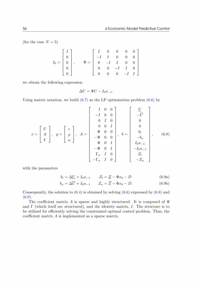
56 6 Economic Model Predictive Control
(for the case N = 5)
I0 =
I
0
0
0
0
, Ψ =
I 0 0 0 0
−I I 0 0 0
0 −I I 0 0
0 0 −I I 0
0 0 0 −I I
we obtain the following expression
∆U = ΨU − I0u−1.
Using matrix notation, we build (6.7) as the LP optimization problem (6.6) by
x =
U
S
V
, g =
c
ρ
α
, A =
I 0 0
−I 0 0
0 I 0
0 0 I
Ψ 0 0
−Ψ 0 0
Ψ 0 I
−Ψ 0 I
Γu I 0
−Γu I 0
, b =
U
−U
0
0
bl−bu
I0u−1
−I0u−1
Zl
−Zu
, (6.8)
with the parameters
bl = ∆U + I0u−1 Zl = Z − Φx0 −D (6.9a)bu = ∆U + I0u−1 Zu = Z − Φx0 −D. (6.9b)
Consequently, the solution to (6.4) is obtained by solving (6.6) expressed by (6.8) and(6.9).
The coefficient matrix A is sparse and highly structured. It is composed of Ψand Γ (which itself are structured), and the identity matrix, I. The structure is tobe utilized for efficiently solving the constrained optimal control problem. Thus, thecoefficient matrix A is implemented as a sparse matrix.

6.5 Implementation 57
6.4.2 SolversSee Chapter 3 for applied solvers in our control framework. Even though it is sig-nificant, a study on solver performances is outside the scope of this thesis. Thereexist many efficient methods for solving linear programs obtained from MPC prob-lems. Also methods utilizing the specific structure, e.g., decomposition methods likeDantzig-Wolfe decomposition returning the master problem into independently sub-problems, which may be solved in parallel [ESJ09; Sok+12; Sok+13]. On a small note,Graphics Processing Unit (GPU) on graphics cards provides exceptional qualities inscientific computations and high-performance computing [DA12].
6.4.3 Optimality conditionsThe optimality conditions for (6.6) will informally be introduced. The Lagrangian of(6.6) is
L(x,λ) = gTx− λT (Ax− b).
Hence, the first order necessary and sufficient optimality conditions may be stated as[NW06]
∇xL(x,λ) = g −ATλ = 0 (6.10a)s−Ax+ b = 0 (6.10b)
SΛ1 = 0 (6.10c)(s,λ) ≥ 0, (6.10d)
where S being the matrix with slack variable s := Ax− b in the diagonal, similarly Λbeing the matrix with Lagrange multiplier in the diagonal, and 1 is a vector will allcomponents one. (6.10c) is the complementarity conditions. The conditions (6.10)are known as the Karush–Kuhn–Tucker conditions.
6.5 Implementation
We outline the developed Matlab implementations of the economic MPC in (6.4).The full implementations are provided in Source Code Booklet Chapter 2. A flowchartof the implementation is illustrated in Figure 6.3. Our implementation is developedas adaptive and generic as possible. Thus, it can be utilized on different simulationscenarios, different system setup (MISO, MIMO), different state-space realizations,etc. This is done to obtain better code quality and a better starting point for furtherresearch and development in this area.
The main script, main_closedloop, contain definition of simulation parameters(e.g., model sampling time steps, number of simulation hours, simulation horizon,and prediction horizon), initialization as well as function calls to developed MPCfunctions. All parameters can easily be modified to achieve the desired simulation. Inthe following, we describe the framework and the purpose of the developed functions.

58 6 Economic Model Predictive Control
• setupSystem set up system model parameters and operational parameters. Inaddition, the system model (e.g., a MIMO system) is defined by applyingcontinuous-time transfer function.
• setupModel realize the model into a discrete-time state-space model.
• setupScenario generate the simulation scenario. Firstly, forecast of powersupply from renewable energy sources (disturbance) is defined. Secondly, theindividual power production as well as the total power production range (tra-jectory for the economic MPC) is determined. Based on the power system,the production plan for each power plant is derived by solving the UC opti-mization problem. The UC optimization problem presented mathematicallyin Section 4.3 by (4.20) is implemented in the function ucSolver and solvedfor global optimality using CPLEX. Lastly, variables for the Kalman filter areinitialized.
• mpcDesign compute and build following: the impulse response matrices by call-ing the function impulseResponse; the input and input rate constraints; A andg of (6.8); the discrete algebraic Riccati equation; and the Kalman filter gains.
These four functions set up the power system and simulation parameters; the offlineMPC. Following represent the online MPC.
• mpcClosedloop perform the closed-loop simulation. The function do following:simulate the system (output measurements from sensor and state simulation);execute the MPC controller algorithm; and store applicable values from theclosed-loop simulation, which are returned. To execute the MPC controlleralgorithm, the function call two functions mpcUpdate and mpcCompute:
– mpcUpdate update the current open-loop MPC matrices. Following are up-dated: current power production range (trajectory) for each power plant;current forecasted power production from renewable energy sources (dis-turbance); input and input rate constraints; and estimates by performingone-step predictor and Kalman filtering by calling the functionupdateStateEstimate.
– mpcCompute, is the regulator, i.e., solve the open-loop MPC. It build thenon-constant vectors and solve the soft constraint economic MPC prob-lem as an linear programming problem by calling the lpSolver. The ob-tained solution is return and feed into the system for each simulation step.lpSolver is a interface for solving linear optimization problems. Threesolvers are supported: CPLEX, MOSEK, and Gurobi; see Chapter 3, thereis to be selected in the main script, main_closedloop.
The results, the historical values returned by mpcClosedloop, is then illustrated usingvarious developed MPC plot functions.
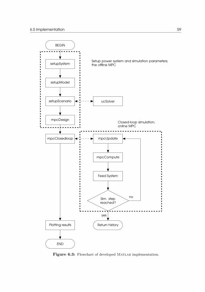
6.5 Implementation 59
BEGIN
setupSystem
setupModel
setupScenario
mpcDesign
mpcClosedloop mpcUpdate
mpcCompute
Feed System
Sim. stepreached?
Return history
ucSolver
Plotting results
END
yes
no
Setup power system and simulation parameters;the offline MPC
Closed-loop simulation;online MPC
Figure 6.3: Flowchart of developed Matlab implementation.

60 6 Economic Model Predictive Control
6.6 Case study
In this section, we establish a power system to demonstrate the formulated soft con-strained economic MPC (6.4) with dynamics of a power plant modeled as presentedin Section 5.2. Firstly, we present the case study and operational parameter of powerplants. Secondly, open-loop and closed-loop simulations are performed. Source codeis listed in Source Code Booklet Section 2.2 and Section 2.3. [HEJ10] inspired to thecase study.
6.6.1 2-unit power systemTwo power plants with different operational features are controlled. Table 6.4 liststhe controller parameters. The parameters are chosen such that power plant 1 ischeap and slow, whereas power plant 2 is expensive and fast. We consider the MISOformulation of the power plants presented in Section 5.2. For convenience the modelis given below
Zi(s) =1
(τis+ 1)3Ui(s), i = 1,2. (6.11)
The total production isZ(s) = Z1(s) + Z2(s). (6.12)
We perform simulations with and without the regularization term to show its impactto the solution. We apply the economic optimizing MPC (6.4), where the system isrealized in a discrete-time state-space form with a sampling time of Ts = 1 seconds;thus, system dynamics are captured. The objective is to minimize operation costsubject to obey demand load and various operational requirements.
6.6.1.1 Open-loop and closed-loop simulations
The results of an open-loop simulation without regularization term is illustrated inFigure 6.5. Figure 6.5(a) shows that the total power production satisfy the prede-fined demand load. The cheapest power plant, plant 1, produces the majority of theload, whereas the more expensive and fast power plant, plant 2, operates wheneverfaster dynamics are required. This behavior is expected considering the operationalparameter of the power system. Figure 6.5(b) and Figure 6.5(c) show that the inputconstraints are satisfied and active at some time periods. We see excessive movementof input for particular plant 2, which may not be desirable due to wear and tear of
Table 6.4: Operational parameters.
Unit τ c ρ α uk uk ∆uk ∆uk
1 20 1 1.0 · 102 0.5 0 10 -1 12 10 2 1.0 · 102 1.0 0 10 -3 3

6.7 Summary 61
the systems. In order to manage these movements, the regularization term may beadded to the objective function.
Figure 6.6 shows the results of an open-loop simulation with the same setup asbefore, but with the regularization term for excessive movement of the input addedto the objective function. There are no significantly changes in the production plan;however, Figure 6.6(c) and Figure 6.6(c) show significant changes in inputs and rateof movement for plant 2. As desirable, we obtain nearly same solution but with lesschange in inputs. Henceforth, the regularization term is included.
At the same setup as before, we execute a closed-loop simulation with predictionhorizon N = 50 time step. The results of the simulation, reported in Figure 6.7, showsnearly same solution as obtained in the open-loop simulation Figure 6.6. However,Figure 6.7(b) and Figure 6.7(c) show that the inputs are not as smooth as in theopen-loop. Increasing the prediction horizon will smooth this and in fact lead thesolution closer to the open-loop simulation. This is expected as we do not utilize thequality of closed-loop simulation, since no valuable feedback information is obtained.
6.7 Summary
This chapter motivates the choice of economic MPC as control framework and givesan introduction to MPC. We formulate a soft constraint linear economic MPC. Weoutline the controller algorithm for an economic MPC with external forecasts andfiltered state estimators computed by a Kalman filter. It is showed how to convert andsolve the optimization problem as a LP optimization problem. We informally presentliterature on stability of economic MPC problems and solvers as well as stating theoptimality conditions for a LP problem. The developed Matlab implementationfor our economic MPC control framework is presented. Lastly, we demonstrate theformulation to a power system. The case studies demonstrated open-loop and closed-loop simulations and that the implementation behaves as expected.

62 6 Economic Model Predictive Control
0 50 100 150 200 250 300 350 400 450 5000
10
20
Tot
al P
ower
[MW
]
Power production Demand load range
0 50 100 150 200 250 300 350 400 450 500
0
5
10
Pla
nt #
1 [M
W]
0 50 100 150 200 250 300 350 400 450 500
0
5
10
Pla
nt #
2 [M
W]
Time [h]
(a) Power productions from the two power plants and total production satisfying demand load range.
0 50 100 150 200 250 300 350 400 450 500
0
2
4
6
8
10
Pla
nt #
1
Input u
min/u
max
0 50 100 150 200 250 300 350 400 450 500
0
2
4
6
8
10
Time [h]
Pla
nt #
2
(b) System inputs with its limits.
0 50 100 150 200 250 300 350 400 450 500
−1
−0.5
0
0.5
1
Pla
nt #
1
∆ Input ∆ u
min/∆ u
max
0 50 100 150 200 250 300 350 400 450 500−4
−2
0
2
4
Time [h]
Pla
nt #
2
(c) Rate of movement for inputs with its limits.
Figure 6.5: Open-loop simulation of a power system without regularization term for ex-cessive movement of the input. Ts = 1.

6.7 Summary 63
0 50 100 150 200 250 300 350 400 450 5000
10
20
Tot
al P
ower
[MW
]
Power production Demand load range
0 50 100 150 200 250 300 350 400 450 500
0
5
10
Pla
nt #
1 [M
W]
0 50 100 150 200 250 300 350 400 450 500
0
5
10
Pla
nt #
2 [M
W]
Time [h]
(a) Power productions from the two power plants and total production satisfying demand load range.
0 50 100 150 200 250 300 350 400 450 500
0
2
4
6
8
10
Pla
nt #
1
Input u
min/u
max
0 50 100 150 200 250 300 350 400 450 500
0
2
4
6
8
10
Time [h]
Pla
nt #
2
(b) System inputs with its limits.
0 50 100 150 200 250 300 350 400 450 500
−1
−0.5
0
0.5
1
Pla
nt #
1
∆ Input ∆ u
min/∆ u
max
0 50 100 150 200 250 300 350 400 450 500−4
−2
0
2
4
Time [h]
Pla
nt #
2
(c) Rate of movement with its limits.
Figure 6.6: Open-loop simulation of a power system with regularization term for excessivemovement of the input. Ts = 1.

64 6 Economic Model Predictive Control
0 50 100 150 200 250 300 350 400 450 5000
10
20
Tot
al P
ower
[MW
]
Power production Demand load range
0 50 100 150 200 250 300 350 400 450 500
0
5
10
Pla
nt #
1 [M
W]
0 50 100 150 200 250 300 350 400 450 500
0
5
10
Pla
nt #
2 [M
W]
Time [h]
(a) Power productions from the two power plants and total production satisfying demand load range.
0 50 100 150 200 250 300 350 400 450 500
0
2
4
6
8
10
Pla
nt #
1
Input u
min/u
max
0 50 100 150 200 250 300 350 400 450 500
0
2
4
6
8
10
Time [h]
Pla
nt #
2
(b) Inputs to the system with its limits.
0 50 100 150 200 250 300 350 400 450 500
−1
−0.5
0
0.5
1
Pla
nt #
1
∆ Input ∆ u
min/∆ u
max
0 50 100 150 200 250 300 350 400 450 500−4
−2
0
2
4
Time [h]
Pla
nt #
2
(c) Rate of movement with its limits.
Figure 6.7: Closed-loop economic MPC simulation of a power system. Prediction horizonis N = 50 time step with regularization term. Ts = 1.

Part IIIUnit Commitment and
Economic ModelPredicetive Control for
Power Systems

CHAPTER 7Introduction
This part present simulation of combining the UC optimization problem and theeconomic MPC problem in the application of optimal operation of power systems.
In this chapter, we provide an overview of the chapters that follows. In Section 7.1and Section 7.2, we describe the developed control strategy and informally discuss re-flection of combining the two methods. Section 7.3 provides the background materialfor the simulations that follows.
An outline of the individual chapters is as following:
Chapter 8 provides a simulation of the impact discretization and input parameter-ization have on the achievable outcome in terms of power imbalance and costs.
Chapter 9 provides simulations of combining the UC problem and the economicMPC problem without power supply from renewable energy sources in the powersystem.
Chapter 10 provides simulations of combining the UC problem and the economicMPC problem with power supply from renewable energy sources in the powersystem.
Chapter 9 and Chapter 10 starts with an overview of the perform simulations andends with a summary of key findings from the simulations.
7.1 Developed control strategy
The aim for the novel coupling of the UC problem and economic MPC problem isto develop a control strategy that intelligently can overcome some of the challengesfor managing the growing uncertainty associated with increasing penetration of non-controllable renewable energy sources into the power grid. Chapter 1 and Chapter 2motivates and discuss some of the challenges with renewable energy sources.
In the following, we present key features of the UC problem and economic MPCproblem underpinning for the developed control strategy outlined subsequent.

68 7 Introduction
UC problem. The UC problem is an intuitive and effective model for optimalpower production planning. In order to intercept the variations in power supply fromthe renewable energy sources and thereby plan the power production accordingly, wewant to solve the UC problem with a high frequency. However, for power systemswith practical size (large-scale power systems), the high computational complexitymakes it impossible to solve the UC problem with a high frequency.
Economic MPC. The economic MPC advantage is the real-time optimization,which can be solved with a high frequency. In addition, economic MPC can anticipatefuture events and take action accordingly. Consequently, the variations in powersupply from renewable energy sources can be taking into account by reoptimizing theproduction plan.
Combining UC and economic MPC. With that in mind, the developed controlstrategy considers the two methods at two distinct levels, as depicted in Figure 7.1.The hierarchy structure is following:
• Day-ahead planning: Firstly, day-ahead planning is performed on a coarse timegrid. Based on available forecasts of tomorrow demand load and power supplyfrom renewable energy sources, the UC problem derive the production plan forthe next 24 hours. The UC solution determine which power plants there arecommitted and decommitted (binary decisions) and the production level at thecommitted plants in an economic effective way (economic dispatch).
• Minutes-ahead planning: Secondly, online minutes-head planning is performedduring the day of operations on a high resolution time grid. Based on updatedand more reliable forecasts of power supply from renewable energy sources, theeconomic MPC reoptimize the production plan in an economic effective way.Thus, we obtain a balance controller there adjust to fluctuations and avoid theundesirable imbalance.
This strategy utilizes the benefits from each of the two methods. We have chosen tosolve the UC problem once every 24 hour. The frequency of solving the UC problem,e.g., periodically every six hours, is a very interesting discussion, however, this willonly be briefly touched upon in this thesis.
7.2 Considerations for combining UC and economic MPC
The UC problem and the economic MPC are not completely the same problem. There-fore, some considerations and decisions need to be made. In the following, we listsome of the differences.
• System dynamics are considered and modeled in the economic MPC, not in theUC problem.

7.2 Considerations for combining UC and economic MPC 69
• The discretization is different for the two methods. In the literature, the UCproblem is modeled and solved with a very coarse discretization, usually hour byhour. Whereas the economic MPC is modeled and solved with a high resolutiondiscretization, sampling time Ts. Usually, the sampling time is chosen small inorder to capture system dynamics.
• The input parameterization is different for the two methods. This opens aquestion of how we apply the plants operational parameters in the UC andeconomic MPC. In our simulations, we want the operational features to beidentical for both methods. Therefore, we perform a direct conversion with thediscretization in account.
• The decision of which power plants there are committed and decommitted foreach time step is solely determined by the UC problem. The described eco-nomic MPC in Chapter 6 does not include binary decisions. Consequently, thecontroller only reoptimizes the production plan and do not decide whether aplant shall startup or shutdown in a time period.
The considerations and challenges evokes interesting discussion and questions, forwhich will be addressed in the following simulations.
Day-ahead Planning UnitCommitment
Economic MPCMinutes-ahead Planning(Online Control)
Power Plant
Figure 7.1: Control strategy of combining the UC and the economic MPC.

70 7 Introduction
Plant 1 Plant 2 Wind Farm
Load (MW)
Figure 7.2: Power system with two controllable conventional power plants and a non-controllable predictable power generator, farms of wind turbines.
7.3 Background for the simulations
In this section, we present the considered power system, the considered demand loads,the operational parameters used in the UC problem and economic MPC, as well asthe initialization.
The power system is inspired from the UC and economic MPC case studies inSection 4.6 and Section 6.6, respectively. We consider the power grid illustratedin Figure 7.2; in details see Figure 5.4. The power grid includes two controllableconventional power plants and a non-controllable predictable power generator, farmsof wind turbines. The wind farm represents the penetration of intermittent renewableenergy sources into the power grid for which we cannot control.
As a remark, we will not consider capacity and distribution challenges in thepower grid. Thus, we assume sufficient capacity and distribution possibility in termsof power plants and renewable energy sources.
7.3.1 Demand loadWe will consider two distinct demand loads in Chapter 9 and Chapter 10. Fig-ure 7.3(a) represents a demand load requiring both power plants to be committedover the 24-hour planning horizon; we refer to busy demand load. Figure 7.3(b) repre-sent a demand load where one power plant is decommitted in a time period; we referto idle demand load. The idle demand load show how our implementation managethe situation when plants shutdown and startup within the 24-hour planning horizon.In Appendix B Table B.1(a) present both demand loads numerically. The spinningreserve is set as a 10% of the demand load for each time period.
Demand load is naturally continuous in time. As Figure 7.3 indicates, the demandload is discretized hour by hour. In Chapter 8, we discover that the discretization havean impact on the solution. We want to investigate various setups impact on performs.Therefore, in order to not account for discretization loss in all the simulations, theeconomic MPC receive the coarse demand load as the UC problem. In a practicalsetting, one should not apply a coarse discretized demand load to the controller,

7.3 Background for the simulations 71
4 8 12 16 20 24600
800
1000
1200
1400
1600
1800T
otal
Pow
er [M
W]
Time [h]
Demand load Spinning reserves
(a) Busy demand load.
4 8 12 16 20 24600
800
1000
1200
Tot
al P
ower
[MW
]
Time [h]
(b) Idle demand load.
Figure 7.3: 24-hour demand load [MW]; see Table B.1(a) in Appendix B for the numericalrepresentation. Spinning reserve is 10% of demand load for each time period.
since it will imply unnecessary information loss. Furthermore, it is assumed that thedemand load do not develop over time, i.e., the demand load is the same for theday-ahead planning as well as the day of operation. These choices eventually onlyhave a negative effect on the economic MPC performances. Thus, if removed, thecontroller will offhand obtain a better solution, and hence a stronger argument forthis strategy to be compelling.
If not otherwise stated, the controller is set to at least satisfy the demand loadgiven to the UC optimization problem; let zk denote the demand load at time stepk, then
zk ≤ zT,k ≤ ∞,
where zk is the total power output at time step k. ∞ denote an upper limit whichis not reached. The reason for this decision is to achieve a fair basis of comparisonwhen comparing the results obtained by the two methods, UC optimization problemand the economic MPC.

72 7 Introduction
Table 7.4: Operational parameters to the UC problem.
Unit ai bi SUi SDi PLi PUi RDi RUi
[$/h] [$/MWh] [$/h] [$/h] [MW] [MW] [MW/h] [MW/h]1 1000 15 10 10 150 850 200 2002 500 30 8 8 150 850 600 600
7.3.2 Operational parametersThe two conventional power plants are modeled to have different operational features.The parameters are chosen such that power plant 1 is cheap and slow, whereas powerplant 2 is expensive and fast. We want the used operational features to be identicalfor both methods. We have chosen to perform a direct conversion of the units. E.g.,the UC variable cost is given in [$/MWh], then, the economic MPC variable cost isdetermined by converting the data into [$/(MW·Ts)].
7.3.2.1 UC parameters
The UC optimization problem presented mathematically in Section 4.3 by (4.20) issolved for global optimality in a open-loop manner. We use IBM ILOG CPLEX Op-timizer V12.6 Matlab interface for solving the UC optimization problem. Table 7.4lists the operational parameters for the UC problem. The spinning reserve is set as a10% of the demand load for each time period.
7.3.2.2 Economic MPC parameters
The economic optimizing MPC presented mathematically in Section 6.3 by (6.4) issolved for global optimality in a closed-loop manner. We use Gurobi Optimizer V5.6Matlab interface for solving the LP optimization problem. The other implementedsolvers have been tested to find the same solution. The controller considers the linearsystem presented in Section 5.2. Thus, the power plants dynamics are modeled by athird order model and the dynamics for the wind farms are neglected due to the quickdynamics of wind turbines. The system is realized in a discrete-time state-space formwith a sampling time of Ts = 20 seconds. The sampling time is chosen such thatsystem dynamics are captured. In closed-loop simulations are the prediction horizonN = 100 time step. Table 7.5 lists the operational parameters for the economic MPC.
We find it more important to satisfy the overall demand load than satisfying theindividual plants production plan given by the UC, thus, we penalize more heavilyon this parameter:
ρi,k = [ρ1,k,ρ2,k,ρT,k] = [10,10,100], (7.1)
where i = 1,2, . . . ,nu and ρT,k is the penalty associated to the overall demand load.The listed penalties, ρ and α, are subject to change during the simulations; in thatcase, it will be explicitly given.

7.3 Background for the simulations 73
Table 7.5: Operational parameters to the economic MPC. Penalty ρi,k = [ρ1,k,ρ2,k,ρT,k] =[10,10,100], where i = 1,2, . . . ,nu and ρT,k is the penalty associated to theoverall demand load.
Unit τ c α uk uk ∆uk ∆uk
[$/(MW·Ts)] [$/Ts] [MW] [MW] [MW/Ts] [MW/Ts]1 20 0.0833 0.0417 150 850 -1.1111 1.11112 10 0.1667 0.0833 150 850 -3.3333 3.3333
7.3.2.3 Initialization
The performed simulations are initialized in following manner. The day-ahead plan-ning is determined by solving the UC problem. We assume no prior knowledge;consequently, the problem is initialized such that power output at time period t = 0is zero,
pi,0 = 0 ∀i,
and the plants status preceding the first period is switch off,
ui,0 = 0 ∀i.
The controller is initialized by applying the obtained solution from the UC problem attime period t = 0. Thus, the UC problem determine which plants there are committedand decommitted.

74
CHAPTER 8Discretization andParameterization
In the literature, the UC optimization problem is modeled and solved with a verycoarse time discretization and without system dynamics. This evokes some questionsas, e.g., has the discretization and parameterization an impact on the achievableoutcome in terms of power imbalance and costs. In the following, we set up a testcase to show the interesting aspects.
We consider a 2-unit power system with the operational parameters given in Sec-tion 7.3.2. Since this is a very computationally expensive task and due to limitedmemory, we perform a 12-hour simulations.
8.1 Discretization
We define following two demand loads:
• Dth with a high resolution grid, one value for each minutes.
• Dtc with a coarse grid, one value for each hour.
Let Dth be the true demand load and Dtc be the discretized version of Dth. Assumethe production to be piecewise constant (ZOH approximation). We investigate theimpact of discretization and input parameterization in the UC optimization problemby following approach:
1. Solve UC using Dth. Let UCth denote the solution. Simulate the solution UCthand derive the associated total amount of production.
2. Solve UC using Dtc. Let UCtc denote the solution. Simulate the solution UCtcon the high resolution grid and derive the associated total amount of production.
3. Solve economic MPC problem with rolling horizon on the high resolution gridusing Dth as trajectory. Let EMPCth denote the solution. Derive the associatedtotal amount of production.
Figure 8.1 illustrates UCtc, UCth, and EMPCth. We present some initial key findings

76 8 Discretization and Parameterization
0 2 4 6 8 10 12600
800
1000
1200
Tot
al P
ower
[MW
]
Time [h]
UC
thUC
tcEMPC
th
(a) Total power production.
0 2 4 6 8 10 12
200
400
600
800
Pla
nt #
1 [M
W]
0 2 4 6 8 10 12
200
400
600
800
Pla
nt #
2 [M
W]
Time [h]
UCth
UCtc
EMPCth PL/PU
(b) Plants power production.
Figure 8.1: Power production obtained from UCth, UCtc, and EMPCth.
• The two UC solutions, UCth and UCtc, are exactly the demand loads, Dth andDtc, respectively.
• In Figure 8.1(b), we see that the cheapest power plant, plant 1, produces themajority of the load, whereas the more expensive and fast power plant, plant2, operates whenever faster dynamics are required. This behavior is expected
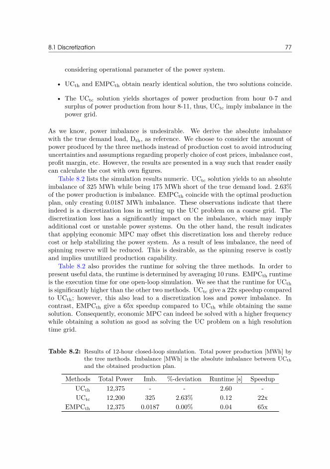
8.1 Discretization 77
considering operational parameter of the power system.
• UCth and EMPCth obtain nearly identical solution, the two solutions coincide.
• The UCtc solution yields shortages of power production from hour 0-7 andsurplus of power production from hour 8-11, thus, UCtc imply imbalance in thepower grid.
As we know, power imbalance is undesirable. We derive the absolute imbalancewith the true demand load, Dth, as reference. We choose to consider the amount ofpower produced by the three methods instead of production cost to avoid introducinguncertainties and assumptions regarding properly choice of cost prices, imbalance cost,profit margin, etc. However, the results are presented in a way such that reader easilycan calculate the cost with own figures.
Table 8.2 lists the simulation results numeric. UCtc solution yields to an absoluteimbalance of 325 MWh while being 175 MWh short of the true demand load. 2.63%of the power production is imbalance. EMPCth coincide with the optimal productionplan, only creating 0.0187 MWh imbalance. These observations indicate that thereindeed is a discretization loss in setting up the UC problem on a coarse grid. Thediscretization loss has a significantly impact on the imbalance, which may implyadditional cost or unstable power systems. On the other hand, the result indicatesthat applying economic MPC may offset this discretization loss and thereby reducecost or help stabilizing the power system. As a result of less imbalance, the need ofspinning reserve will be reduced. This is desirable, as the spinning reserve is costlyand implies unutilized production capability.
Table 8.2 also provides the runtime for solving the three methods. In order topresent useful data, the runtime is determined by averaging 10 runs. EMPCth runtimeis the execution time for one open-loop simulation. We see that the runtime for UCthis significantly higher than the other two methods. UCtc give a 22x speedup comparedto UCth; however, this also lead to a discretization loss and power imbalance. Incontrast, EMPCth give a 65x speedup compared to UCth while obtaining the samesolution. Consequently, economic MPC can indeed be solved with a higher frequencywhile obtaining a solution as good as solving the UC problem on a high resolutiontime grid.
Table 8.2: Results of 12-hour closed-loop simulation. Total power production [MWh] bythe tree methods. Imbalance [MWh] is the absolute imbalance between UCthand the obtained production plan.
Methods Total Power Imb. %-deviation Runtime [s] SpeedupUCth 12,375 - - 2.60 -UCtc 12,200 325 2.63% 0.12 22x
EMPCth 12,375 0.0187 0.00% 0.04 65x

78 8 Discretization and Parameterization
8.2 Parameterization
Now, let us dwell on the operational parameters and the input parameterizationof UC problem. Consider Figure 8.1(b). We see that the system increase powerproduction at plant 1 as much as possible as fast as possible and the reverse at plant2. Consequently, plant 1 ramp-up constraint are active until maximum power output,PU1 = 850 MW, is attained. UCtc power production is constant between hoursand when the power level change is it accomplished within 0 second. E.g., plant1 increase the power level with RU1 = 200 MW within 0 seconds at hour 1, 2, 3,and 4. In between, the production is constant. This evolution occurs because of therepresentation of the UC problem; however, how should it be interpreted? Considerfollowing two cases:
1. the power level can increase reality fast (0-10 minutes); or
2. the power level cannot increase that fast and use nearly an hour to attainmaximum ramp-up.
Case 1 indicates nonoptimal utilization of the power plants capabilities. If the ramp-up is fast, the power level may as well increase again within 1 hour instead of waitinguntil next hour. Case 2 indicates that the used parameterization in the UC problemis not appropriate compared to the physical plant. If the ramp-up is not instantlybut rather as a slope, then, the parameterization should be so.
8.3 Key findings
The findings in this section show that the discretization and input parameterizationhave a cost impact on the solution. EMPCth solution coincide with the optimalproduction plan while UCtc solution yields 2.63% imbalance power of the total powerproduction. Furthermore, EMPCth give a 65x speedup compared to UCth whileobtaining the same solution. A deeper analysis and research may find hidden costsavings and unutilized resources. Maybe traditions have surpassed research.
An interesting perspective: the total production cost by UCtc solution is 2.63%subject to additional cost by imbalance cost. In Section 4.6.2, we considered a 10-unitpower system. In this case study, the startup and shutdown cost where less than 1%of the total production cost. Consequently, if it is important to include startup andshutdown cost in the objective function when solving the UC optimization problem,then, it must likewise be interesting to look closely on discretization loss.

CHAPTER 9Deterministic
SimulationsIn this chapter, we present simulations of combining the UC problem and the economicMPC problem without power supply from renewable energy sources in the powersystem. We perform following simulations:
• Apply MISO formulation in the controller
• Apply MIMO formulation in the controller
– Use system power output limits as trajectory– Use the UC solution as trajectory
Section 5.2 provides the MISO and MIMO formulation. In all cases, 24-hour closed-loop simulations are performed considering the two demand load provided in Sec-tion 7.3.1. The obtained production plan from solving the UC problem is included inthe illustrations. Lastly, we present key findings from the performed simulations.
9.1 MISO simulations
In this section, the MISO system formulation is applied. The economic MPC objectiveis to minimize operation cost while satisfying the predefined demand load subject tosystem limits.
The results of the simulation with the busy demand load are reported in Figure 9.1.The production plan found by the economic MPC follow the UC solution with theexception of system dynamics included in the MPC framework.
Figure 9.1(b) shows that the cheapest power plant, plant 1, produces the majorityof the load, whereas the more expensive and fast power plant, plant 2, operates when-ever faster dynamics are required. This behavior is expected considering operationalparameter of the power system. An interesting observation is that the economic MPCconstantly increase power production on plant 1 until maximum power output on 850MW is reached. This illustrate the discussion about used input parameterization inthe UC problem; see Chapter 8. The small drops in EMPC production for plant 1 isdue to the dynamics of the system when power level changes. If this is not desirable

80 9 Deterministic Simulations
in practice, one can adjust control parameters accordingly to reduce them, e.g., byincrease penalty of excessive movement of the input.
The performed inputs to the system and the rate of movement, reported in Fig-ure 9.2, shows that the constraints are satisfied and are active at some time periods.Particularly, the power plants ability to ramp-up and ramp-down is a limit in thesimulation.
The results of the simulation with the idle demand load are reported in Figure 9.3.Our implementation can handle the case when power plants change from committedto decommitted and vice versa. We set u = 0 and PL = 0 at decommitted hourswhereas u = 0 and PU = 0 one hour after and before shutdown and startup such thatthe system is not penalties due to system dynamics. Around shutdown and startupthe economic MPC solution differ from the UC solution; e.g., Figure 9.3(b) at hour4 to 5. The UC increase power production on the expensive plant 2 since otherwiseit will be impossible to decrease the power level to 600 MW at hour 6. In contrast,the EMPC increase the power production on the cheap plant 1. This is possible dueto the system dynamics and parameterization of the economic MPC
The performed inputs to the system and the rate of movement, reported in Fig-ure 9.4, shows that the constraints are satisfied and are active at some time periods.Again, the power plants ability to ramp-up and ramp-down is a limit in the simulation.Additionally, we see that there is no input to plant 2 when it is decommitted.

9.1 MISO simulations 81
0 4 8 12 16 20 24
800
1000
1200
1400
Tot
al P
ower
[MW
]
Time [h]
EMPC UC Demand load
(a) Total power production.
0 4 8 12 16 20 24
200
400
600
800
Pla
nt #
1 [M
W]
0 4 8 12 16 20 24
200
400
600
800
Pla
nt #
2 [M
W]
Time [h]
EMPC UC PL/PU
(b) Plants power production.
Figure 9.1: 24-hour MISO closed-loop simulation applying the busy demand load as tra-jectory. UC production profile for power plants are unknown while committedplants are known for the economic MPC.

82 9 Deterministic Simulations
0 4 8 12 16 20 24
200
400
600
800
Pla
nt #
1
Input u
min/u
max
0 4 8 12 16 20 24
200
400
600
800
Time [h]
Pla
nt #
2
(a) System inputs with its limits.
0 4 8 12 16 20 24
−1
−0.5
0
0.5
1
Pla
nt #
1
∆ Input ∆ u
min/∆ u
max
0 4 8 12 16 20 24−4
−2
0
2
4
Time [h]
Pla
nt #
2
(b) Rate of movement for inputs with its limits.
Figure 9.2: 24-hour MISO closed-loop simulation applying the busy demand load. Per-formed inputs to the system and the rate of movement together with theirlimits.

9.1 MISO simulations 83
0 4 8 12 16 20 24
600
700
800
900
1000
Tot
al P
ower
[MW
]
Time [h]
EMPC UC Demand load
(a) Total power production.
0 4 8 12 16 20 24
200
400
600
800
Pla
nt #
1 [M
W]
0 4 8 12 16 20 24
0
200
400
600
800
Pla
nt #
2 [M
W]
Time [h]
EMPC UC PL/PU
(b) Plants power production.
Figure 9.3: 24-hour MISO closed-loop simulation applying the idle demand load as trajec-tory. UC production profile for power plants are unknown while committedplants are known for the economic MPC.

84 9 Deterministic Simulations
0 4 8 12 16 20 24
200
400
600
800
Pla
nt #
1
Input u
min/u
max
0 4 8 12 16 20 24
0
200
400
600
800
Time [h]
Pla
nt #
2
(a) System inputs with its limits.
0 4 8 12 16 20 24
−1
−0.5
0
0.5
1
Pla
nt #
1
∆ Input ∆ u
min/∆ u
max
0 4 8 12 16 20 24−4
−2
0
2
4
Time [h]
Pla
nt #
2
(b) Rate of movement for inputs with its limits.
Figure 9.4: 24-hour MISO closed-loop simulation applying the idle demand load. Per-formed inputs to the system and the rate of movement together with theirlimits.
9.2 MIMO simulations 85
9.2 MIMO simulations
In this section, the MIMO system formulation is applied. The economic MPC objec-tive is to minimize operation cost while satisfying the predefined demand load andpower plants trajectory subject to system limits. Two different ways of modeling thetrajectories are presented. In Section 9.2.1, we let the UC problem determine thecommitted and decommitted plants while the production plan (economic dispatch) isentirely controlled by the economic MPC. In Section 9.2.2, we let the UC problemdetermine the committed and decommitted plants as well as the production plan forthe individual power plants, which the controller is set to obey.
9.2.1 System power output limits as trajectoryThis simulation uses the UC problem to determine the committed and decommittedplants. The production plan is entirely controlled by the economic MPC to be withinsystem power output range, PL = 150 MW and PU = 850 MW. Thus, the optimalproduction plan obtained by the UC is unknown for the economic MPC; however, forcomparing purpose are the solutions shown.
Firstly, we consider the busy demand load. Figure 9.5 illustrates the total powerproduction and the power production on each power plant. The obtained resultsare comparable to previous simulations in Section 9.1. Thus, same observations areapplicable.
Secondly, we consider the idle demand load. This simulation differs from theone in Section 9.1 in terms of setup. The MIMO formulation provide the abilityto control the power plants independently, which underlies the reason for applyingthis formulation, as described in Section 5.2. In the case of decommitted plants, themanipulable input range is zero as well as the plants individual trajectory. We setu = 0 at decommitted hours whereas u = 0 one hour after and before shutdown andstartup. The plants trajectory is set to zero, i.e., PL = PU = 0, in all decommittedhours. Thus, penalty is added if power is produced in decommitted hours. Theresults of the simulation, reported in Figure 9.6, show faster response when plant 2startup at hour 21. This leads to following: shorter production time on the expensiveplant 2; longer production time on the cheap plant 1; a higher overshoot in the totalpower production; and less rate of input movement for plant 2 (see Figure 9.4(b)).All findings are due to the economic MPC ability to set the trajectories and penaltiesto push the solution towards the desired behavior.

86 9 Deterministic Simulations
0 4 8 12 16 20 24
800
1000
1200
1400
Tot
al P
ower
[MW
]
Time [h]
EMPC UC Demand load
(a) Total power production.
0 4 8 12 16 20 24
200
400
600
800
Pla
nt #
1 [M
W]
0 4 8 12 16 20 24
200
400
600
800
Pla
nt #
2 [M
W]
Time [h]
EMPC UC PL/PU
(b) Plants power production.
Figure 9.5: 24-hour MIMO closed-loop simulation applying the busy demand load andsystem power output limits as trajectories. UC production profile for powerplants are unknown while committed plants are known for the economic MPC.

9.2 MIMO simulations 87
0 4 8 12 16 20 24
600
700
800
900
1000
Tot
al P
ower
[MW
]
Time [h]
EMPC UC Demand load
(a) Total power production.
0 4 8 12 16 20 24
200
400
600
800
Pla
nt #
1 [M
W]
0 4 8 12 16 20 24
0
200
400
600
800
Pla
nt #
2 [M
W]
Time [h]
EMPC UC PL/PU
(b) Plants power production.
Figure 9.6: 24-hour MIMO closed-loop simulation applying the idle demand load andsystem power output limits as trajectories. UC production profile for powerplants are unknown while committed plants are known for the economic MPC.

88 9 Deterministic Simulations
9.2.2 Individual production plans as trajectoryThis simulation uses the UC problem to determine the committed and decommittedplants as well as the individual production plan for the power plants. The economicMPC is set to obey these production plans. This introduces a new way of controllingthe power production. Now, the controller can be forced to be close to the demandload, close to the individual production plans for the power plants, or a combinationof the two. Thus, many combinations are possible. We set a range around the plansby shifting the power level for each time periods either by a fixed amount [MW] orby a percents of the power level. The range for the power plants is set to ±60 MWand the demand load range is set to ±100 MW for each time period.
The results of the simulation with the busy demand load and the idle demand loadare reported in Figure 9.7 and Figure 9.8, respectively. The economic MPC producethe minimum allowed power during the 24 hours. It still produced maximum powerat plant 1 while the production is decreased at plant 2. This result is as expected.
Besides the lower power production, the result differs from Section 9.2.1 when therange is reached. E.g., consider the first few hours. Figure 9.7(b) shows that plant1 and 2 have small plateau compared to Figure 9.5(b) where plant 1 have a steadypower increase until maximum power output is attained and plant 2 have a moresteep power decrease. This demonstrates that introducing individual ranges enablesthe possibility to manage the power production on each power plants as desired andthereby secondarily satisfy the overall demand load. Meanwhile, the controller ensuresto find the minimum production cost subject to system limits.

9.2 MIMO simulations 89
0 4 8 12 16 20 24600
800
1000
1200
1400
1600
Tot
al P
ower
[MW
]
Time [h]
EMPC UC Demand load range
(a) Total power production.
0 4 8 12 16 20 24
200
400
600
800
Pla
nt #
1 [M
W]
0 4 8 12 16 20 24
200
400
600
800
Pla
nt #
2 [M
W]
Time [h]
EMPC UC Plant range
(b) Plants power production.
Figure 9.7: 24-hour MIMO closed-loop simulation applying the busy demand load. Theeconomic MPC is to obey obtained production plan from solving the UCproblem within a defined range (trajectories).

90 9 Deterministic Simulations
0 4 8 12 16 20 24
600
800
1000
Tot
al P
ower
[MW
]
Time [h]
EMPC UC Demand load range
(a) Total power production.
0 4 8 12 16 20 24
200
400
600
800
Pla
nt #
1 [M
W]
0 4 8 12 16 20 24
0
200
400
600
Pla
nt #
2 [M
W]
Time [h]
EMPC UC Plant range
(b) Plants power production.
Figure 9.8: 24-hour MIMO closed-loop simulation applying the idle demand load. Theeconomic MPC is to obey obtained production plan from solving the UCproblem within a defined range (trajectories).

9.3 Key findings 91
9.3 Key findings
We perform simulations of combining the UC problem and the economic MPC prob-lem without power supply from renewable energy sources in the power system. Boththe MISO and MIMO formulation of the power system were applied in the controller.We demonstrate that our economic MPC implementation can follow the solution fromthe UC problem.
The MIMO formulation provides benefits in terms of the possibility for individualcontrol of the power plants while collaborate to satisfy a common objective, the overalldemand load. Section 9.2 present two different setups, which are useful dependingon the situations and purpose. Introducing individual ranges around the UC solutionenables endless possibilities to manage the power production. Consequently, the exactway of coupling the UC problem and economic MPC should be situation and purposedependent.

92

CHAPTER 10Stochastic Simulations
In this chapter, we perform simulations of combining the UC problem and the eco-nomic MPC problem with power supply from renewable energy sources in the powersystem. The controller consider the MIMO system; see Section 5.2. The power supplyfrom renewable energy sources are modeled as following:
• Wind power modeled as a step
• Wind power modeled as a fluctuating function, a sine wave
In our simulations, we let the UC determine the committed and decommitted plantswhile the production plan is entirely controlled by the economic MPC to be withinsystem power output limits. Lastly, we present key findings from the performedsimulations.
10.1 Modeling forecasts of wind power supply
We model the power production from the wind turbines as a composition of threevalues each representing the layer of knowledge and reliability of the forecasts. Let
• dst1 denote the day-ahead forecasts of wind power production;
• dst2 denote the adjusted forecasts of wind power production obtainable duringthe day of operations; and
• dst3 denote the necessary adjustments to obtain the true power wind powerproduction the day of operations.
Then, we model
dstUC = dst1 (10.1a)dstEMPC = dstUC + dst2 (10.1b)
dstSim = dstEMPC + dst3. (10.1c)
dstUC is the forecast applied to the UC problem. dstEMPC is the forecast for theeconomic MPC in a receding horizon manner, and dstSim is the disturbance measuredby sensor. dstSim is the true wind power production. This approach of modeling the

94 10 Stochastic Simulations
wind production offers the opportunity to simulate the real-world forecasts. Since, astime goes, more information is available and forecasts will be more reliable. However,forecasts are embedded with some uncertainties, which means that some fluctuationswill occur between the best wind power production forecast and the true wind powerproduction, which is modeled by the unknown disturbances, dst3.
10.2 Step wind power
We investigate the system response when power supply from renewable energy sourcesinstantly change from initial forecasted. We consider following two cases:
1. Wind contribution is known for the economic MPC though dk+j|k in (6.4). Thissimulates the situation where updated and more reliable wind forecasts areprovided to the economic MPC.
2. Wind contribution is unknown and modeled as a disturbance. Thus, the eco-nomic MPC identify the disturbance from the measurements. This simulatesthe situation of unexpected wind power production.
For both cases, the wind production is unknown at the time the UC is solved. 6-hourclosed-loop simulations are performed considering the busy demand load. At hour 3,150 MW wind power enter the system. As new information is available, the requiredproduction for the plants will be changed. Hopefully, the set-point change will bedetected by the economic MPC due to the rolling horizon and feedback, and hencechange the power production accordingly. In the opposite case where less wind poweris received than initially forecasted, the system response will just be the reversed.
10.2.1 Case 1The results of the 6-hour simulation, reported in Figure 10.1, show that the controllerreact to the set-point change at hour 3, whereas the production plan derived from theUC yields into unnecessary power production. The actual required power generatedby the plants is represented by the solid cyan line. Figure 10.1(b) shows that theeconomic MPC reduce the power production at plant 1 when the wind power enteringthe system. This is to be expected, since the production at the expensive plant 2cannot be reduced further due to the minimum power output limit.
We see the controllers ability to react to changes when new and more reliableinformation is available. In addition, we also see a challenge with the controller.The economic MPC do not include binary decisions, as the planning regarding whichplants there are committed and decommitted is determined by the UC. Consequently,surplus of power may occur if following is true: 1) power supply from renewableenergy sources change a lot compared to initial forecasts, and 2) the system cannotdecrease the production further due to minimum power output limits. In that case,a shutdown of a power plant may be a good decision. This indicates that solving theUC problem ones the day-ahead may not be the optimal solution.

10.2 Step wind power 95
0 1 2 3 4 5 6
700
800
900
1000
1100T
otal
Pow
er [M
W]
Time [h]
EMPC UC Required power Demand load
0 1 2 3 4 5 60
50
100
150
Win
d P
ower
[MW
]
Time [h]
dstEMPC
dstSim
(a) Top: Total power production from the UC and the economic MPC. Required power generatedby plants (solid cyan). Bottom: Wind power production.
0 1 2 3 4 5 6
200
400
600
800
Pla
nt #
1 [M
W]
0 1 2 3 4 5 6
200
400
600
800
Pla
nt #
2 [M
W]
Time [h]
EMPC UC PL/PU
(b) Plants power production.
Figure 10.1: 6-hour closed-loop simulation when 150 MW wind power entering the systemat hour 3.

96 10 Stochastic Simulations
10.2.2 Case 2The results of 6-hour simulation, reported in Figure 10.2(a), show that the controllerdo not react in the same manner as before. The production is reduced but nowherenear enough. We obtain this phenomenon, since the disturbance is not modeled inour control framework. In order to remove offset and hence obtain offset free control,we model an unmeasured disturbance model by incorporating an output disturbanceinto the process model; see Section 5.5.
Figure 10.2(b) illustrates the same setup as before, but with offset free MPC.Now, a much better solution is obtained, as the controller reacts on the unexpectedset-point change and decrease power production accordingly. We see interesting MPCcharacteristics around hour 3. As we know, the control framework is solved in a rollinghorizon manner and in each time step look N prediction steps ahead. Therefore,increases the power production towards hour 3 to prepare for the increasing demandload at hour 3. After hour 3, the required power production to satisfy the demandload deceases because of the sudden wind power supply. By measurements from thephysical plant, the controller gets new information and adapt to the changed situation.Consequently, we obtain a peak at hour 3. Figure 10.1(a) show no peak at hour 3,because the controller gets the new update information prior the set-point change.
In this simulation, we identified MPC ability to anticipate future events and totake actions accordingly when disturbance entering the system by the closed-loopfeedback. In the rest of our simulations, we apply offset free MPC.

10.2 Step wind power 97
0 1 2 3 4 5 6
700
800
900
1000
1100
Tot
al P
ower
[MW
]
Time [h]
EMPC UC Required power Demand load
0 1 2 3 4 5 60
50
100
150
Win
d P
ower
[MW
]
Time [h]
dstEMPC
dstSim
(a) Top: Total power production from the UC and the economic MPC. Required power generatedby plants (solid cyan). Bottom: Wind power production model as disturbance to the system.
0 1 2 3 4 5 6
700
800
900
1000
1100
Tot
al P
ower
[MW
]
Time [h]
EMPC UC Required power Demand load
(b) Offset free MPC simulation. Same setup and wind power disturbance profile as Figure 10.2(a).
Figure 10.2: 6-hour closed-loop simulation with the busy demand load. Figure 10.2(a)shows the result of offset MPC simulation and Figure 10.2(b) shows theresult of offset free MPC. Both with same simulation setup.

98 10 Stochastic Simulations
10.3 Fluctuating wind power
We investigate the system response when power supply from renewable energy sourcesis modeled to be fluctuating. Based on our acquired experience from above, we applythe offset free MPC presented in Section 5.5. We consider following four cases:
1. First example of introducing fluctuating non-controllable predictable wind powerproduction.
2. Examine the impact wind power have on power system imbalance by fixingthe frequency, the fluctuations of the wind power, and vary the amplitude, theamount of wind power production.
3. The opposite as above: fixing the amplitude, the amount of wind power pro-duction, and vary the frequency, the fluctuations of the wind power.
4. Introduce stochastic process noise and measurements noise.
In following simulations, we apply the busy demand load from Figure 7.3(a). However,the discretization setup is changed for the economic MPC. Now, the controller receivesthe demand load represented on the high resolution time grid. Figure 10.3 depictedthe demand load on the coarse grid and high resolution grid.
In order to test our implementations ability to adapt to a fluctuating trajectoryis the forecast generated by the sine wave function (10.2). The sine wave functionis chosen since this function gives a smooth repetitive oscillation. The sine wave isdefined as a function of time, t, in the form:
f(t) = α sin(
2πωt
24 · 60
), (10.2)
4 8 12 16 20 24600
800
1000
1200
1400
1600
1800
Tot
al P
ower
[MW
]
Time [h]
Demand load
tcDemand load
th Spinning reserves
Figure 10.3: 24-hour demand load [MW]. Coarse grid demand load (tc) applied in theUC problem (solid blue) and high resolution demand load (th) applied inthe economic MPC (solid cyan). Spinning reserve is 10% of demand loadtcfor each time period.

10.3 Fluctuating wind power 99
0 4 8 12 16 20 24−2
0
2
dstUC
dstEMPC
dstSim
0 4 8 12 16 20 24−1
0
1
dst1
0 4 8 12 16 20 24−1
0
1
dst2
0 4 8 12 16 20 24−1
0
1
Time [h]
dst3
Figure 10.4: Example illustration of (10.1) applying (10.2).
where α is the amplitude and ω is the frequency. Figure 10.4 illustrates an exampleof the computed (10.1) applying (10.2). We chose to fix the ratio between dst1, dst2,and dst3. It is preliminary clear that if the day-ahead wind power production forecast,dst1, is embedded with more uncertainty, the performance difference between the UCproblem and the economic MPC will be to the controllers advantage.
As we know, the discretization is different for the two methods. The applied windpower forecasts, dstUC, dstEMPC, and dstSim, are derived on high resolution timegrid. Then, dstUC is discretized, hour by hour, to fit the discretization in the UCoptimization problem. We calculate the discretization as the mean value for eachhour; thus, at each hour the production level is shift up or down.
10.3.1 Case 1The wind power supply is modeled by (10.2) using the parameters listed in Table 10.5.
The results of 6-hour simulation, reported in Figure 10.6, show many interestingaspects. As expected, the UC solution return into imbalance situation due to thediscretization and the change in wind power production during the day of operations.

100 10 Stochastic Simulations
Table 10.5: Applied parameters in Figure 10.6 to (10.2).
Forecasts α ω
dst1 50 0.1dst2 25 0.4dst3 12.5 0.8
0 1 2 3 4 5 6600
800
1000
1200
Tot
al P
ower
[MW
]
Time [h]
EMPC UC Required power
0 1 2 3 4 5 6−100
−50
0
50
100
Win
d P
ower
[MW
]
Time [h]
dstUC
dstEMPC
dstSim
Figure 10.6: 6-hour closed-loop simulation. Top: Total power production from the UCand the economic MPC. Required power generated by plants (solid red).Bottom: Wind power production defined as (10.1).
Meanwhile, the economic MPC nicely follow the required power production by thetwo plants to satisfy the demand load. In some situations, the economic MPC cannotfollow the fast changes; e.g., between hour 2 and 3. The imbalance as function of time,reported in Figure 10.7, show how good the economic MPC solution is compared tothe UC solution.

10.3 Fluctuating wind power 101
0 1 2 3 4 5 6
−150
−100
−50
0
50Im
bala
nce
[MW
]
Time [h]
EMPC UC
Figure 10.7: Imbalance as function of time for simulation Figure 10.6. Calculated as thedifferences between the optimal required power production by plants andthe two derived solutions: UC solution and economic MPC solution.
10.3.2 Case 2
We fix the frequency, the fluctuations of the wind power, and vary the amplitude, theamount of wind power production. We want to consider the impact of wind powerhave on power system imbalance. We calculate the absolute imbalance between theoptimal production and the derived. We choose to consider the amount of power pro-duced instead of production cost to avoid introducing uncertainties and assumptionsregarding properly choice of cost prices, imbalance cost, profit margin, etc. However,results will be presented in a way such that reader easily can calculate the cost withown figures.
Table 10.8: Results of 24-hour closed-loop with four different amplitudes. Imbalance isthe absolute imbalance between the optimal production and the obtainedproduction plan.
α Methods Total Power [MWh] Imb. [MWh] %-deviation- Optimal 27,150 - -
0 UC 27,100 1,150 4.24%EMPC 27,150 0.07 0.00%
14 UC 27,100 1,169 4.31%EMPC 27,155 10 0.04%
35 UC 27,100 1,219 4.49%EMPC 27,175 37 0.14%
70 UC 27,100 1,356 5.00%EMPC 27,267 152 0.56%

102 10 Stochastic Simulations
24-hour closed-loop simulations are performed with four different amplitudes,
α = {0,14,35,70}
and the frequency,ω = {dst1,dst2,dst3} = {0.1,0.4,0.8} .
Because of the way we model wind power production, the total power productionobtained by the optimal power production will numerical be the same in all four sim-ulations. The same is true of the UC optimization problem. This does not necessarilyapply for the absolute imbalance.
Table 10.8 lists the obtained results of the simulations. In all cases, the economicMPC obtain a better solution than the UC problem, nearly identical to the optimal.Without wind power production, α = 0, the UC solution yields to 4.24% of the powerproduction is imbalance while the comparable economic MPC solution coincide withthe optimal. The only differences between the two methods are the discretization.Thus, in this example, the discretization loss is significant. As α increases, the imbal-ance increases for the two methods. In particular, we see that the controller beginsto have difficulties to follow the very fluctuating wind power production. Furtherresearch of control parameters may optimize the results. In the hardest case, α = 70,the amount of imbalance the controller produce only stands for 0.56% of the totaloptimal power production, whereas the solution from the UC optimization problemyields 5%.
The obtained solution with α = 14 and α = 70 are depicted in Figure 10.9. Theillustrations confirm the data analyzed before. In Figure 10.9(b), we see that thecontroller has difficulties to follow in some cases when fluctuations are too large. Wenote that penalty is added if the controller produce less than demand load

10.3 Fluctuating wind power 103
0 4 8 12 16 20 24600
800
1000
1200
1400
1600T
otal
Pow
er [M
W]
Time [h]
EMPC UC Required power
0 4 8 12 16 20 24−40
−20
0
20
40
Win
d P
ower
[MW
]
Time [h]
dstUC
dstEMPC
dstSim
(a) α = 14.
0 4 8 12 16 20 24600
800
1000
1200
1400
1600
Tot
al P
ower
[MW
]
Time [h]
EMPC UC Required power
0 4 8 12 16 20 24−200
−100
0
100
200
Win
d P
ower
[MW
]
Time [h]
dstUC
dstEMPC
dstSim
(b) α = 70.
Figure 10.9: 24-hour closed-loop simulation with two different amplitude values. Top:Total power production from the UC and the economic MPC. Requiredpower generated by plants (solid red). Bottom: Wind power productiondefined as (10.1).

104 10 Stochastic Simulations
10.3.3 Case 3
We fix the amplitude, the amount of wind power production, and vary the frequency,the fluctuations of the wind power. Two 6-hour simulations are performed where thefrequency is doubled. The wind power production is modeled by (10.2) using theparameters listed in Table 10.10.
The results of the simulations are reported in Figure 10.11. The economic MPCobtain a decent result. As the frequency increases, the controller has difficulties insome time periods to follow the optimal power production completely due to theintegrated system dynamics and limits. The economic MPC solution follows theupper peaks, because penalty is added if production is below the demand load.
In the following, we set the power output range to be ±0.03% of the demand load.Figure 10.12 shows the result with ω2 (the same simulation as in Figure 10.11(b)).Now, the production plan is more in the middle and do not necessarily follow theupper (nor the lower) peaks. Consequently, control parameters may be adjusted inorder to obtain the desired behavior.
10.3.4 Case 4
Now, we take a step back. We want to show an interesting challenge with uncer-tainties. The utilized data and forecasts are not incontestable and thus embeddedwith some uncertainties. E.g., forecasts of demand load, forecasts of renewable en-ergy supply, forecasts of prices, etc. Additionally, in scientific computing where wetry to simulate the real-world, model uncertainties are also present. If uncertaintiesbecome a significant part of provided data, time should be spent on investigating theemerging challenges.
As we know, one of the reasons to apply MPC for optimal control of systems is itsgreat feature of getting close to system limits without exceeding. However, this maybecome a challenge if uncertainties are significant. We note that it is very expensiveto exceeding system limits, as it may result in stability issue and possible breakdownsin the power grid. In present simulations, we have seen that the controller increasethe power production at plant 1 to its maximum power output. In the following,we apply significant process and measurement noise into the system to show thatthis may be an issue. Let the noise in the system be uncorrelated and identically
Table 10.10: Applied parameters in Figure 10.11(a) and Figure 10.11(b) to (10.2).
Forecasts α ω1 ω2
dst1 50 0.2 0.4dst2 25 0.8 1.6dst3 12.5 1.6 3.2

10.4 Key findings 105
independently normally distributed as wk
ξkvk
∼ Niid
0
0
0
,
82 0 0
0 82 0
0 0 202
. (10.3)
6-hour closed-loop simulation, reported in Figure 10.13, show that the demand loadis not satisfied in all time steps. The economic MPC find a feasible solution, sincethe output constraints are soften, thus, penalty is added. Furthermore, we see thatplant 1 exceed its maximum power output in the last hours.
The purpose of this simulation is to show that uncertainties may be an issuein practices. An investigation on these challenges is outside the scope of this the-sis. However, we would like to mention a possible way to address this issue. Thestochastic uncertainties may be modeled into the economic MPC model. The Mean-Variance economic MPC include the mean and variance of the data [Sok+14; Cap+15;Mor+14]. E.g., consider the production cost cTu, where c is the prices of producingpower. Then, we may formulate the objective as
minimize{u}
ϕ = λE[cTu] + (1− λ)Var[cTu], λ ∈ [0,1]. (10.4)
E[cTu] is the expected value of the cost and Var[cTu] is the variance of the cost. λis a risk aversion parameter that determines the trade-off between the expected costand the cost variance.
10.4 Key findings
We perform simulations of combining the UC problem and the economic MPC prob-lem with power supply from renewable energy sources in the power system. We iden-tify MPC ability to anticipate future events and to take actions accordingly whendisturbance entering the system by the closed-loop feedback. Thus, as new and morereliable information is available, the controller reoptimizes the production plan. Weobserve that modeling the unmeasured disturbance, by incorporating an output dis-turbance into the process model, yields nicely behavior and we obtain offset freeMPC.
Simulations indicate that the solutions obtained by the economic MPC are betterthan the solution obtained by the UC optimization problem. Less power imbalance iscreated using economic MPC. As the fluctuations can be managed by the controller ina predictive manner, the need for reserve capacity is reduced. This implies potentialcost reduction with a good impact on the environment.
Furthermore, we address some challenges with the controller when the renewablepower supply is fluctuating too much too fast and when introducing uncertainties indata or model. These challenges are interesting, because too fluctuating power supplymay result into undesirable imbalance and unstable power systems.

106 10 Stochastic Simulations
0 1 2 3 4 5 6600
800
1000
1200T
otal
Pow
er [M
W]
Time [h]
EMPC UC Required power
0 1 2 3 4 5 6−100
−50
0
50
100
Win
d P
ower
[MW
]
Time [h]
dstUC
dstEMPC
dstSim
(a) Simulation with ω1 presented in Table 10.10.
0 1 2 3 4 5 6600
800
1000
1200
Tot
al P
ower
[MW
]
Time [h]
EMPC UC Required power
0 1 2 3 4 5 6−100
−50
0
50
100
Win
d P
ower
[MW
]
Time [h]
dstUC
dstEMPC
dstSim
(b) Simulation with ω2 presented in Table 10.10.
Figure 10.11: 6-hour closed-loop simulation. Fixed amplitude and vary frequency. Windpower modeled by (10.2) using parameters listed in Table 10.10.

10.4 Key findings 107
0 1 2 3 4 5 6600
700
800
900
1000
1100
Tot
al P
ower
[MW
]
Time [h]
EMPC UC Required power
0 1 2 3 4 5 6−100
−50
0
50
100
Win
d P
ower
[MW
]
Time [h]
dstUC
dstEMPC
dstSim
Figure 10.12: Same simulation as Figure 10.11(b) with the change of power output rangeto be ±0.03% of the demand load.

108 10 Stochastic Simulations
0 1 2 3 4 5 6600
800
1000
1200
Tot
al P
ower
[MW
]
Time [h]
EMPC Demand load
(a) Total power production.
0 1 2 3 4 5 6
200
400
600
800
Pla
nt #
1 [M
W]
0 1 2 3 4 5 6
200
400
600
800
Pla
nt #
2 [M
W]
Time [h]
EMPC Plant range
(b) Plants power production.
Figure 10.13: 6-hour closed-loop simulation. Consider the stochastic model with stochas-tic process noise and measurements noise distributed as (10.3).

Part IVConclusions and
Perspectives


CHAPTER 11Conclusions and
PerspectivesIn this thesis, we have investigated the design and implementation of combing theUnit Commitment (UC) optimization problem and the economic Model PredictiveControl (MPC) problem for optimal operation of power systems. This chapter willcollect the key findings presented in the thesis and provide concluding remarks, aswell as address possible extensions and directions for future research.
The thesis primary objective is repeated: By combining the unit commitment opti-mization problem and the economic model predictive control problem, it is possible toobtain an intelligent control strategy that can overcome some of the important chal-lenges associated with the increasing share of intermittent renewable energy sources inthe power supply. This novel coupling will operate the power systems in a cost efficientmanner while satisfying the overall demand load and various system requirements.
We have shown that the developed novel control strategy appears to provide afeasible and a promising solution to overcome some of the important challenges. Weprovide an intelligent control strategy that shows properties of managing uncertaintywith flexibility. We demonstrate a potential for significant savings in imbalance cost.
Reliable forecasts of power supply from renewable energy sources are of greatimportance, since the uncertainties in these forecasts have a significantly impact onthe imbalance cost and stability issues. We demonstrate the importance of reoptimizethe production plan during the day of operation in order to account for fluctuationsand reducing the dependence on the correctness of forecasts. We show that economicMPC is indeed an appealing method to enable for this functionality. By real-timeoptimization with feedback, economic MPC successfully adapt, predict, and changethe production plan according to the fluctuations inherent in renewable power supply.A reduction in imbalance will also lead to less need of the expensive spinning reserve,which again yields cost savings and have a good impact on the environment.
Conclusively, the provided valuable learning will without a doubt be interestingto the academia and industry like DONG Energy.
112 11 Conclusions and Perspectives
11.1 UC
In Chapter 4, we describe and formalize mathematically the UC optimization prob-lem as a mixed integer linear programming problem. UC is an intuitive methodto determine the optimal production plan for a giving portfolio of power generatingplants. Scheduling with a financial and environmental perspective is nontrivial. Thecomplexity is a key challenge for this type of problem. Generally, UC is NP-complete.Consequently, for power systems with practical size (large-scale power systems), thehigh computational complexity makes it impossible to solve the UC problem with ahigh frequency, in order to intercept the variations inherent in the nature of renewableenergy sources.
11.2 Economic MPC
Chapter 5 introduce the principles of models for predictive control including realisticlinear dynamical model of power plants in a power system. Furthermore, we introducemodel for achieving offset free tracking performance in the presences of unmeasurednonzero disturbances; representation of dynamics by the Finite Impulse Response(FIR) model; as well as Kalman state estimation, filtering, and prediction subject tostochastic noise.
In Chapter 6, we motivate the choice of economic MPC as our control framework,as well as describe and formalize mathematically a soft constrained linear economicMPC framework into a linear optimization programming problem. In our work, weconsider both a deterministic and a stochastic formulation.
MPC capability to integrate predictions and forecasts of dynamical systems, aswell as anticipate future events and take control actions accordingly are receivedeagerly, since this is exactly the functionality we require. Compared to the UCoptimization problem, the economic MPC is designed to be solved in real-time ata high frequency, with updated and more reliable forecast as input.
11.3 UC and economic MPC
We present a two-level control strategy: At the high-level, the day-ahead productionplan is performed on a coarse time grid (e.g., hourly) by solving the UC problem. Atthe low-level, the minutes-ahead production plan, or the online control, is performedon a high resolution time grid (e.g., 20 sec) by applying the economic MPC.
In Chapter 8, a case study indicates that the coarse discretization for the UC havea cost impact on the solution. Compared to the optimal production plan, the UCsolution with coarse discretization yields 2.63% imbalance power while the economicMPC solution coincide with the optimal production plan. Simultaneous, the economicMPC have a runtime of 0.04 sec. Solving the UC problem on a high resolution timegrid yields a runtime of 2.60 sec. Thus, we obtain a 65x speedup. This supports thechoice of using economic MPC as the method for reoptimizing the production plan.

11.3 UC and economic MPC 113
In Chapter 9, we observe that our economic MPC implementation yields great track-ing performance. The provided MIMO formulation enables the controller the oppor-tunity to manage each power plant independently while tracking them to satisfy acommon goal, e.g., obey the overall demand load. This formulation enables endlesstuning and setup possibilities to manage the power production as desirable whileminimizing the operating cost subject to system limitations.
In Chapter 10, we examine the system reaction when intermittent renewable energysources enter the power system. The results show that the controller indeed have theability to anticipate future events and to take actions accordingly, when disturbanceenter the system. We identified the importance of formulating the economic MPCto achieve offset free tracking performance, when unmeasured nonzero disturbanceentering the system.
We address some challenges for the controller when the renewable power supplyis fluctuating too much too fast and when introducing uncertainties in the data ormodel. The latter is particular interesting. MPC great feature of operating thesystem to its limits may introduce challenges if data or forecasts are embedded withsignificant uncertainty. By simulations, we show that system limits may be exceededin the event of significant process noise and measurement noise. Therefore, we suggestincorporating uncertainties into the control framework

114 11 Conclusions and Perspectives
11.4 Perspectives and further research
The subject of this thesis is far more extensive than the scope of the thesis. There aretwo paths to be followed after this project. One path is to test the control strategysuitability in a practical setting by an industrial implementation maturing. Theother path is further academic development. In the following, we address possibleextensions and directions for future research.
• Further development, design prototypes, and real-life testing will definitelyprove the feasibility and verify the initial results of an economic and environ-mental potential.
• In Chapter 8, results show that the UC discretization and parameterization havea significant impact on the cost. Further investigation should be conducted todetermine whether there exists hidden cost savings and unutilized resources.
• We solve the UC once at the day-ahead planning. Maybe changing the cyclesyield a better performance, e.g., executing the UC problem in a closed-loopmanner with rolling-shrinking horizon approach. Then, apply the economicMPC to balancing the production in between. Thus, the controller is reset bya new and updated UC solution.
• Initial results show that the developed control framework may have some chal-lenges if data or model uncertainties are significant. Therefore, for the controlstrategy to be applicable one may look on how to handle these uncertaintiesappropriately. It might also be interesting to examine the formulation of theeconomic MPC objective. E.g., one could formulate
α ∥uk − uk∥+ (1− α) ∥∆uk∥ ,
where uk is the manipulated variables, uk is the trajectory from solving theUC optimization problem, and α is a risk aversion parameter that determinesthe trade-off between following the UC solution and the cost of discouragesdisproportionate movement of the manipulable variables. In addition, we modelthe cost function as a linear cost. If the costs more correctly follow a nonlinertrend, the change to nonlinear economic MPC may introduce new issues assolution time, stability issues, and robustness [JYB14; Luc+14].
• The electricity market does not really match to the current and future way ofproducing power. The market should maybe be modified to better fit the newway of power production. We see that the intraday market has come increasinglyimportant as more renewable energy sources enter the power grid. Imbalancebetween day-ahead contracts and actually produced often need to be offset.By curious, the electricity is a commodity production there can be bought,sold, and traded. Rather comparable to the financial market where financialsecurities are traded. Thus, can we imagine a scenario where stocks and alikeonly were traded once a day?

Part VAppendices


APPENDIX ABackground Material
This appendix present mathematical background, results, and theorems applied inthis thesis.
A.1 Linearization and discretization
This section outlines the basic concepts of how a linear time-invariant continuous-timemodel may be linearized and discretized to obtain a linear time-invariant discrete-time state-space model. For simplification, an example of a deterministic nonlineardynamical system will be considered.
A.1.1 Continuous-time state-space modelThe deterministic nonlinear dynamical system may be stated in terms of ordinarydifferential equations
x(t) = f(x(t), u(t), d(t)), x(t0) = x0 (A.1a)y(t) = g(x(t)) (A.1b)z(t) = h(x(t)). (A.1c)
Approximating (A.1) using Taylor expansion around the equilibrium point(xs,us,ds,ys,zy) defined by
f(xs,us,ds) = 0
ys(t) = g(xs)
zs(t) = h(xs),
yields the corresponding linear time-invariant continuous-time state-space model
X(t) = AX(t) +BU(t) + ED(t), X(t0) = X0 (A.3a)Y (t) = CX(t) (A.3b)Z(t) = CzX(t), (A.3c)

118 A Background Material
G(s)
Gd(s)
U(s)
D(s)
Y (s)
Figure A.1: Input-ouput relation describing the transfer functions.
where the linear system state matrices A, B, C, E, and Cz are computed by
A = ∇xf(xs,us,ds), B = ∇uf(xs,us,ds), E = ∇df(xs,us,ds),
C = ∇xg(xs), Cz = ∇xf(xs).
The deviation variables X(t), U(t), D(t), Y (t), and Z(t) are defined by
X(t) = x(t)− xs, U(t) = u(t)− us, D(t) = d(t)− ds,
Y (t) = y(t)− ys, Z(t) = z(t)− zs.
Notice that the system state matrices can be time-varying. The stochastic continuous-time state-space representation of this is
X(t) = AX(t) +BU(t) + ED(t) +GW (t)
Y (t) = CX(t) + V (t)
Z(t) = CzX(t).
A.1.2 Continuous-time transfer functionThe linear time-invariant continuous-time system (A.3) with the initial conditionX(0) = 0 and Y ≡ Z can be represented as the input-output function in the Laplacedomain
Y (s) = G(s)U(s) +Gd(s)D(s),
where U(s) is the input function, Y (s) the output function, D(s) the disturbancefunction, and G(s) and Gd(s) are the transfer functions. Figure A.1 is a block diagramof the input-output relation. The transfer functions G(s) and Gd(s) describe therelation between input and output of the system, thus,
G(s) = C(sI −A)−1B
Gd(s) = C(sI −A)−1E,

A.1 Linearization and discretization 119
where I is the identity matrix. Various continuous-time transfer functions exists. Twoexamples are given below:
G(s) =K
(τs+ 1)n
G(s) =K(βs+ 1)
(τ1s+ 1)(τ2s+ 1).
A system respond time to an input can be modeled by adding a time-delay term tothe transfer function. We obtain the transfer function
G(s) =Y (s)
U(s)e−τds.
Examples,
G(s) =K
(τs+ 1)ne−τds
G(s) =K(βs+ 1)
(τ1s+ 1)(τ2s+ 1)e−τds.
Systems with multiple input and multiple output may be described by set of transferfunctions. E.g., the transfer function for a system with two inputs and one output, aMISO system, is
Y (s) =[G1(s) G2(s)
] [ U1(s)
U2(s)
].
A.1.3 Discrete-time state-space modelThe model describing the dynamical systems, independent of realization, can be dis-cretized into a discrete-time state-space model. Let the input, U(t), be piecewiseconstant. This is the case when the input is determined by a computer. We assumea zero-order hold (ZOH) discrete sampling. Let Ts be the sampling time, such thatthe sampling instants, tk, are
tk = t0 + kTs, k = 0,1,2, . . . ,
the zero-order hold of the inputs be characterized by
U(t) = Uk, tk ≤ t < tk+1,
and the states at discrete times X(tk) = Xk. Then, the linear time-invariant continuous-time system (A.3) is equivalent with the linear time-invariant discrete-time state-space model
Xk+1 = AdXk +BdUk + EdDk, X(tk) = Xk (A.7a)Yk = CdXk (A.7b)Zk = Cz,dXk, (A.7c)

120 A Background Material
with
Ad = eATs , Bd =
∫ Ts
0
eAτBdτ, Ed =
∫ Ts
0
eAτEdτ,
Cd = C, Cz,d = Cz.
Ad, Bd, and Ed are computed using the matrix exponential with sampling period Ts
by Ad(Ts) Bd(Ts) Ed(Ts)
0 I 0
0 0 I
= exp
A B E
0 0 0
0 0 0
Ts
.
The discrete-time linear time-invariant system (A.7) can be represented as the input-output function in the Z-domain; see Appendix A.2.3.
The subscript d to explicit indicate discrete-time state-space matrices will beskipped as we only consider discrete-time state-space systems. Consequently, weformulate the deterministic linear time-invariant discrete-time state-space model by
xk+1 = Axk +Buk + Edk +Gwk (A.9a)yk = Cxk (A.9b)zk = Czxk. (A.9c)
and the stochastic linear time-invariant discrete-time state-space model by
xk+1 = Axk +Buk + Edk +Gwk (A.10a)yk = Cxk + vk (A.10b)zk = Czxk, (A.10c)
where xk denotes the states, uk the manipulated input variables, yk the measuredoutputs, zk the controlled outputs, wk the stochastic process noise, and vk the mea-surement noise. dk is the process disturbance that can be predicted by a prognosis andare predicted independently of the measurements y. Consequently, dk shall be con-sidered as the non-controllable power contribution from, e.g., wind power production,which in some sense can be predicted by weather forecasts.
Additionally, models used by the predictive controller may be obtained by systemidentification, e.g., from experimental analysis; that is, fitting a transfer function toexperimental observations obtained by performing a step or impulse response of thesystem. Although, system identification is a very important theme, it is beyond thisthesis scope.

A.2 List of used theorems 121
A.2 List of used theorems
The following sections list used theorems.
A.2.1 Propositional logic[RG91] present following propositional logic, which is applied in the thesis.
P ⇒ Q ⇔ ¬P ∧Q. (A.11)
De Morgan’s theorem
¬(P ∧Q) ⇔ ¬P ∨ ¬Q (A.12a)
and
¬(P ∨Q) ⇔ ¬P ∧ ¬Q. (A.12b)
A.2.2 Laplace transformThe Laplace transform is a linear operator that transform a function f(t), t ∈ R≥0,to a function F (s), s ∈ C, given by the integral [Str08]
F (s) =
∫ ∞
0
f(t)e−stdt. (A.13)
A.2.3 Z-transformZ-transform converts a discrete-time signal sequence x[n] into a complex frequencydomain representation X[z] by
X(z) =
∞∑n=−∞
x[n]z−n, (A.14)
where z = Re(z) + jIm(z).

122

APPENDIX BSystem Data
This appendix present data used in the thesis.

124 B System Data
Table B.1: 24-hour demand load [MW] applied in simulations. Spinning reserve is 10%of demand load for each time period.
(a) Refered as the busy demand load.
Hour Demand loadBusy
1 7002 7503 8504 9505 10006 11007 11508 12009 130010 140011 145012 150013 140014 130015 120016 105017 100018 110019 120020 140021 130022 110023 90024 800
(b) Refered as the idle demand load.
Hour Demand loadIdle
1 7002 7503 8504 9505 10006 6007 6008 6009 60010 60011 60012 60013 60014 60015 60016 60017 60018 65019 70020 75021 80022 90023 100024 1000

BSystem
Data
125
Table B.2: Operational parameters for the 10-unit power system.
Plant ai bi SUi SDi PLi PUi RDi RUi TUi TDi EC
[$/h] [$/MWh] [$/h] [$/h] [MW] [MW] [MW/h] [MW/h] [h] [h] [g/kWh]1 1000 16.19 10 10 150 455 200 200 8 8 7802 970 17.26 10 10 150 455 200 200 8 8 5003 700 16.6 8 8 20 130 100 100 5 5 5004 680 16.5 8 8 20 130 100 100 5 5 5005 450 19.7 8 8 25 162 100 100 6 6 5006 370 22.26 10 10 20 80 50 50 3 3 5007 480 27.74 10 10 25 85 50 50 3 3 5008 660 25.92 8 8 10 55 50 50 1 1 5009 665 27.27 8 8 10 55 50 50 1 1 50010 670 27.79 8 8 10 55 50 50 1 1 500

126
APPENDIX CThe GRANI Program
The GRANI program is a ground-breaking Smart Grid technology on the Faroe Is-lands launched on November 2012. GRANI is a strategic joint venture mainly betweenSEV1 and DONG Energy2 with a budget of approximately DKK 4 million. The pro-gram is part of the European Union, Seventh Framework Programme (FP7), Twen-ties Project, and DONG Energy Power Hub Technology. Following quote present thebackground for the GRANI program:
”Develop and test new technologies for the integration of fluctuating re-newable energy in the isolated electricity network located in the FaroeIslands”.[ND09, §2.1].
The scale of the GRANI program is endless. The achieved experience and knowledgewill be applied in larger power systems such as Denmark for then to introduce intoeven larger systems. The two central goals of the GRANI program are [ND09]:
1. Integration of more renewable energy into the energy system and to serve asa large-scale test facility helping implementation of the EU 2020 vision, whilesolving the world’s energy and climate problems.
2. Opportunity to demonstrate, tests, and develop new solutions for integratingfluctuating renewable energy in an isolated power grid.
Faroe Island produce 14-45 MW power; 60% is produced by expensive heavy fuel oil,35% by hydro power, and only 5% is produced by wind power [NB13]. Accordingto Figure 2.1, has the oil price more than triple the last 10 years. To reduce thedependency on oil and to reduce the carbon footprint, Faroe Island goal is that 75%of the power production in 2020 will come from renewable energy sources [NB13].
Faroe Island is unique as a demo-test case. It is unique in terms of size (50.000inhabitants), location, and power production facilities. The size makes the island toan isolated big city in Denmark. The isolated location in the Atlantic Ocean providesthe island some of the world’s best and worst wind resources; harsh weather conditions
1SEV is Faroe Islands power company owned by the municipalities.2DONG Energy is one of the leading energy groups in Northern Europe there procuring, produc-
ing, distributing, and trading energy products.

128 C The GRANI Program
with frequent storms and very hard to forecast. Furthermore, due to a small powersystem and no interconnections to other counties, the power system is exposed to ahigh number of blackouts when comparing to continental Europe [BND12]. Despitethese challenges the goal is to increase penetration of fluctuating renewable energy,which calls for developing a system that can provide stability, is of great importance.

NomenclatureList of abbreviations
EIA U.S. Energy Information AdministrationEMPC Economic Model Predictive ControlFIR Finite Impulse ResponseFOB Free On Board; a legal trade termKKT Karush–Kuhn–Tucker (conditions)LTI Linear Time-InvariantMILP Mixed Integer Linear ProgrammingMIMO Multiple Input Multiple OutputMIP Mixed Integer ProgrammingMISO Multiple Input Single OutputMPC Model Predictive ControlPL Priority List methodSIMO Single Input Multiple OutputSISO Single Input Single OutputUC Unit CommitmentZOH Zero-Order Hold

130 C The GRANI Program
List of symbols
∀ Logical sign, meaning ”for all”R The real numbersC The complex numbersZ2 The binary number: {0, 1}R≥0 The nonnegative real numbers: {x ∈ R | x ≥ 0}x The minimum/lower value of xx The maximum/upper value of x1 A vector with all components onexT The transpose of a vector or matrix∇ The nabla operator. In the Cartesian coordinate system
Rn with coordinates (x1,x2, . . . ,xn), the nabla operator isdefined in terms of partial derivative operators as ∇ =(
∂
∂x1,
∂
∂x2, · · · , ∂
∂xn
)∥x∥1 ℓ1-norm of a vector x, i.e., ∥x∥1 =
∑nk=1 |xk|, x =
(x1,x2, . . . ,xn)
Symbols used in UC
Indexes:i Plant indext Time period index
Constants:I Total number of power generating plantsT Length of the planning horizonDt System power load demand for time period t
Rt Spinning reserve required at time period t
PWt Forecasted power production from renewable power sourcesat time period t
ai, bi Coefficients of the production cost function of plant i
SUi Startup cost of plant i
SDi Shutdown cost of plant i
PLi Minimum power output generation of plant i
PUi Maximum power output generation of plant i

C The GRANI Program 131
RDi Maximum ramp-down of plant i
RUi Maximum ramp-up of plant i
ECi CO2 emission rate for plant i
EU Maximum CO2 emission allowed
Variables:ui,t Binary variable; 1 if plant i is committed in time period t
and 0 otherwiseyi,t Binary variable; 1 if plant i is started up at the beginning
of time period t and 0 otherwisezi,t Binary variable; 1 if plant i is shutdown at the beginning of
time period t and 0 otherwisepi,t Nonnegative real variable; power output of plant i in time
period t
Symbols used in economic MPC
k Time period indexN Prediction horizonTs Time sampleK Variable gain for transfer functionxk State vectoruk Manipulable input variabledk Disturbanceyk Measured outputzk Controlled outputspk Unmeasured disturbancewk Stochastic process noisevk Stochastic measurement noiseξk Stochastic unmeasured disturbance noiseA, B, C, Cz, F ,Fz, G
Linear system state matrices
Bp, Cp Linear system state matrices for modeling unmeasured dis-turbance, Bp = 0 and Cp = I
Φy, Γyu, Φz, Γzu Linear representation of dynamicsck Cost of producing powersk Slack variable for penalizing term for satisfy demand loadρk Weight for penalizing term for satisfy demand load

132 C The GRANI Program
α Weight for penalizing term for discourages disproportionatemovement of the manipulable variables
Rk Power output rangeDk Power production forecasts from renewable energy sourcesµ Function solve the soft constrained linear economic MPC
optimization problemzk Minimum value of power outputzk Maximum value of power outputuk Minimum value of manipulable inputuk Maximum value of manipulable input∆uk Rate of movement for manipulable input∆uk Maximum ramp-down rate of movement∆uk Maximum ramp-up rate of movement
Kalman filter:Niid The independent and identically normal distributionRww, Rwv, Rvw,Rξ
Variances for process noise, measurement noise, and distur-bance noise
P Discrete algebraic Riccati equation (DARE)Rfe, Kfx, Kfw,Kfp
Innovation covariance and Kalman filter gain and
ek Innovation

Bibliography[AAR12] D. Angeli, R. Amrit, and J. B. Rawlings. On Average Performance and
Stability of Economic Model Predictive Control. In: Automatic Control,IEEE Transactions on 57.7 (July 2012), pages 1615–1626. issn: 0018-9286.
[AC13] O. Adeodu and D. J. Chmielewski. Control of electric power transmissionnetworks with massive energy storage using economic MPC. In: AmericanControl Conference (ACC), 2013. June 2013, pages 5839–5844.
[AH04] D. Axehill and A. Hansson. A preprocessing algorithm for MIQP solverswith applications to MPC. In: Decision and Control, 2004. CDC. 43rdIEEE Conference on. Volume 3. December 2004, 2497–2502 Vol.3.
[And04] G. Andersson. Modelling and analysis of electric power systems. In: EEH-Power Systems Laboratory, Swiss Federal Institute of Technology (ETH),Zürich, Switzerland (2004).
[And12] G. Andersson. Dynamics and control of electric power systems. In: Lecturenotes (2012), pages 227–0528.
[BMM99] A. Bemporad, D. Mignone, and M. Morari. An Efficient Branch andBound Algorithm for State Estimation and Control of Hybrid Systems.In: European Control Conference. Karlsruhe, Germany, August 1999.
[BND12] E. den Boer, C. Nielsen, and H. Djurhuus. Launch of ground break-ing smart grid technology on the Faroe Islands. Invitation by SEV andDONG. Online; Visited AUG 11, 2014. November 2012. url: http://www.twenties-project.eu/system/files/Launch%20of%20ground%20breaking%20smart%20grid%20technology%20in%20the%20Faroese%20Islands.pdf.
[Cap+15] A. Capolei, E. Suwartadi, B. Foss, and J. B. Jørgensen. A mean�varianceobjective for robust production optimization in uncertain geological sce-narios. In: Journal of Petroleum Science and Engineering 125 (2015),pages 23–37. issn: 0920-4105.

134 Bibliography
[Cas+11] E. Castillo, A. J. Conejo, P. Pedregal, R. García, and N. Alguacil. Build-ing and Solving Mathematical Programming Models in Engineering andScience. Pure and Applied Mathematics: A Wiley Series of Texts, Mono-graphs and Tracts. Wiley, 2011. isbn: 9780471461654.
[CM87] P. J. Campo and M. Morari. Robust Model Predictive Control. In: Amer-ican Control Conference, 1987. June 1987, pages 1021–1026.
[Con+11] E. M. Constantinescu, V. M. Zavala, M. Rocklin, S. Lee, and M. Anitescu.A Computational Framework for Uncertainty Quantification and Stochas-tic Optimization in Unit Commitment With Wind Power Generation. In:Power Systems, IEEE Transactions on 26.1 (February 2011), pages 431–441. issn: 0885-8950.
[DA12] P. J. Dinesen and P. E. Aackermann. Development of a GPU-acceleratedMIKE 21 Solver for Water Wave Dynamics. Supervised by AssociateProfessor Allan P. Engsig-Karup, [email protected], DTU Informatics.Asmussens Alle, Building 305, DK-2800 Kgs. Lyngby, Denmark, 2012.url: http://www2.imm.dtu.dk/pubdb/views/publication_details.php?id=6367.
[Dat04] B. N. Datta. Numerical Methods for Linear Control Systems: Design andAnalysis. Numerical Methods for Linear Control Systems: Design andAnalysis vb. 1. Elsevier Academic Press, 2004. isbn: 9780122035906.
[Din10] A. L. Diniz. Test cases for unit commitment and hydrothermal schedulingproblems. In: Power and Energy Society General Meeting, 2010 IEEE.July 2010, pages 1–8.
[DTU] DTU - Technical University of Denmark. Study Handbook: MSc in Math-ematical Modelling and Computation at DTU 2014/2015. url: http ://sdb.dtu.dk/2014/5/59.
[EIAa] EIA U.S. Energy Information Administration. International Energy Out-look 2013; Release Date: July 25, 2013. Visited AUG 25, 2014. url: http://www.eia.gov/forecasts/ieo/world.cfm.
[EIAb] EIA U.S. Energy Information Administration. International Energy Statis-tics. Visited AUG 25, 2014. url: http : / / www . eia . gov / cfapps /ipdbproject/IEDIndex3.cfm.
[EIA14] EIA U.S. Energy Information Administration. Spot prices of crude oiland petroleum products by selected U.S. and international areas. VisitedAUG 13, 2014. August 2014. url: http://www.eia.gov/dnav/pet/PET_PRI_SPT_S1_A.htm.
[EMB09] K. Edlund, T. Mølbak, and J. D. Bendtsen. Simple models for model-based portfolio load balancing controller synthesis. In: Power Plants andPower Systems Control. Volume 1. 1. 2009, pages 173–178.

Bibliography 135
[Enea] Energinet.dk. About the wholesale market. Non-profit enterprise ownedby the Danish Climate and Energy Ministry. Visited DEC 3, 2014. url:http://www.energinet.dk/EN/El/Engrosmarked/Viden-om-engrosmarkedet/Sider/Viden-om-engrosmarkedet.aspx.
[Eneb] Energinet.dk. Vindmøller slog rekord i 2014 (Danish). Non-profit enter-prise owned by the Danish Climate and Energy Ministry. Visited JAN9, 2015. url: http://www.energinet.dk/DA/El/Nyheder/Sider/Vindmoeller-slog-rekord-i-2014.aspx.
[Ene14] Energinet.dk. Smart Grid in Denmark 2.0. Technical Report, Energinet.dk,The Danish TSO owned by the Danish Climate and Energy Ministry. Vis-ited DEC 9, 2014. September 2014. url: http://www.energinet.dk/EN / FORSKNING / Energinet - dks - forskning - og - udvikling / Smart -Grid/Sider/default.aspx.
[ESJ09] K. Edlund, L. E. Sokoler, and J. B. Jørgensen. A Primal-Dual Interior-Point Linear Programming Algorithm for MPC. In: Decision and Control,2009 held jointly with the 2009 28th Chinese Control Conference. CD-C/CCC 2009. Proceedings of the 48th IEEE Conference on. December2009, pages 351–356.
[Eur03] European Commission. The Energy Challenge of the 21st Century: Therole of nuclear energy. 2003. url: ftp://ftp.cordis.europa.eu/pub/fp6/docs/euratom_challenge_21stcentury.pdf.
[Eur13] European Commission. Energy challenges and policy. May 2013. url:http://ec.europa.eu/europe2020/pdf/energy2_en.pdf.
[Gur14] Gurobi Optimization, Inc. Gurobi Optimizer. Visited SEP 20, 2014. 2014.url: http://www.gurobi.com/products/gurobi-optimizer/gurobi-overview.
[GZP03] X. Guan, Q. Zhai, and A. Papalexopoulos. Optimization based methodsfor unit commitment: Lagrangian relaxation versus general mixed inte-ger programming. In: Power Engineering Society General Meeting, 2003,IEEE. Volume 2. IEEE. July 2003.
[Hal+14] R. Halvgaard, J. B. Jørgensen, N. K. Poulsen, and H. Madsen. ModelPredictive Control for Smart Energy Systems. PhD Thesis. Technical Uni-versity of Denmark, 2014.
[HEJ10] T. G. Hovgaard, K. Edlund, and J. B. Jørgensen. The potential of Eco-nomic MPC for power management. In: Decision and Control (CDC),2010 49th IEEE Conference on. December 2010, pages 7533–7538.

136 Bibliography
[Hol+09] H. Holttinen, P. Meibom, A. Orths, F. van Hulle, B. Lange, M. O’Malley,J. Pierik, B. Ummels, J. Tande, A. Estanqueiro, M. Matos, E. Gomez, L.S’oder, G. Strbac, A. Shakoor, J. Ricardo, J. Smith, M. Milligan, and E.Ela. Design and operation of power systems with large amounts of windpower: Final report, IEA WIND Task 25, Phase one 2006-2008. VTTTiedotteita - Research Notes 2493. VTT Technical Research Centre ofFinland, 2009. isbn: 978-951-38-7308-0.
[Hov13] T. G. Hovgaard. Power Management for Energy Systems. PhD Thesis.Technical University of Denmark, February 2013.
[Huu+10] J. K. Huusom, N. K. Poulsen, S. B. Jørgensen, and J. B. Jørgensen. Tun-ing of methods for offset free MPC based on ARX model representations.In: American Control Conference (ACC), 2010. June 2010, pages 2355–2360.
[IBM11] IBM Corporation Software. Modeling Optimization Problems with IBMILOG Cplex Optimization Studio. Visited AUG 28, 2014. 2011. url:https://www-950.ibm.com/events/wwe/grp/grp004.nsf/vLookupPDFs/1_ILOG_Modeling_Examples/$file/1_ILOG_Modeling_Examples.pdf.
[IBM14] IBM Corporation Software. IBM ILOG CPLEX Optimization Studio. Vis-ited AUG 05, 2014. 2014. url: http://www-03.ibm.com/software/products/en/ibmilogcpleoptistud/.
[Jen] M. Jensen. DONG Energy - Power Hub. Asset Manager. Visited DEC 3,2014. url: https://powerhub.dk/.
[JHR11] J. B. Jørgensen, J. K. Huusom, and J. B. Rawlings. Finite Horizon MPCfor Systems in Innovation Form. In: Proceeding of the 50th IEEE Confer-ence on Decision and Control and European Control Conference. IEEE,2011, pages 1896–1903. isbn: 978-1-61284-799-3.
[Jør] J. B. Jørgensen. Smart Energy Systems. Visited DEC 3, 2014. url: http://www.imm.dtu.dk/~jbjo/smartenergy.html.
[Jør05] J. B. Jørgensen. Moving Horizon Estimation and Control. PhD thesis.Department of Chemical Engineering, Technical University of Denmark,2005.
[Jør11] J. B. Jørgensen. Constrained Predictive Control: A Computational Ap-proach. Springer, 2011.
[JYB14] J. J�schke, X. Yang, and L. T. Biegler. Fast economic model predictivecontrol based on NLP-sensitivities. In: Journal of Process Control 24.8(2014). Economic nonlinear model predictive control, pages 1260–1272.issn: 0959-1524.
[KBP96] S. A. Kazarlis, A. G. Bakirtzis, and V. Petridis. A genetic algorithm so-lution to the unit commitment problem. In: Power Systems, IEEE Trans-actions on 11.1 (February 1996), pages 83–92. issn: 0885-8950.

Bibliography 137
[KSH00] T. Kailath, A. H. Sayed, and B. Hassibi. Linear Estimation. Prentice-Hall information and system sciences series. Prentice Hall, 2000. isbn:9780130224644.
[Luc+14] S. Lucia, J. A. E. Andersson, H. Brandt, M. Diehl, and S. Engell. Handlinguncertainty in economic nonlinear model predictive control: A comparativecase study. In: Journal of Process Control 24.8 (2014). Economic nonlinearmodel predictive control, pages 1247–1259. issn: 0959-1524.
[Mac02] J. M. Maciejowski. Predictive Control with Constraints. Prentice Hall,2002. isbn: 9780201398236.
[Mat] MathWorks. MATLAB: Mathematical Computing Software for Engineersand Scientists. url: http://www.mathworks.com/.
[May+00] D. Q. Mayne, J. B. Rawlings, C. V. Rao, and P. O. M. Scokaert. Con-strained model predictive control: Stability and optimality. In: Automatica36.6 (2000), pages 789–814. issn: 0005-1098.
[MB02] K. R. Muske and T. A. Badgwell. Disturbance modeling for offset-freelinear model predictive control. In: Journal of Process Control 12.5 (2002),pages 617–632. issn: 0959-1524.
[MD12] E. Ministry of Climate and B. to the Danish Parliament. Energy policyreport 2012. Technical report. May 2012.
[MNG14] M. G. Marcovecchio, A. Q. Novais, and I. E. Grossmann. Deterministicoptimization of the thermal Unit Commitment problem: A Branch andCut search. In: Computers & Chemical Engineering 67 (2014), pages 53–68. issn: 0098-1354.
[Mor+14] J. M. Morales, A. J. Conejo, H. Madsen, P. Pinson, and M. Zugno. Inte-grating Renewables in Electricity Markets: Operational Problems. Interna-tional Series in Operations Research and Management Science. Springer,2014. isbn: 978-1-4614-9410-2.
[MOS14] MOSEK ApS. MOSEK Optimization Software. Visited SEP 20, 2014.2014. url: http://www.mosek.com/products/mosek.
[NB13] T. Nielsen and A. Birke. Solutions for small power systems. Presentationby SEV and DONG. Visited AUG 11, 2014. January 2013. url: http://www.twenties- project.eu/system/files/13%20Power%20Hub%20Demonstration%20day%20-%20Solutions%20for%20small%20power%20systems%20-%20Terji%20Nielsen,%20SEV%20%26%20Anders%20Birke,%20DONG%20Energy.pdf.
[ND09] C. Nielsen and H. Djurhuus. SEV and Dong Energy put the Faroes onthe world map in electrical energy. SEV and DONG Energy joint ventureagreement. Visited AUG 11, 2014. June 2009. url: http://sev.net.dynamicweb.dk/Default.aspx?ID=1767.

138 Bibliography
[NKF09] T. Niknam, A. Khodaei, and F. Fallahi. A new decomposition approachfor the thermal unit commitment problem. In: Applied Energy 86.9 (2009),pages 1667–1674. issn: 0306-2619.
[Nor] Nord Pool Spot. The Power Market. Visited DEC 3, 2014. url: http://www.nordpoolspot.com/How-does-it-work/.
[NW06] J. Nocedal and S. J. Wright. Numerical Optimization. Springer Seriesin Operations Research and Financial Engineering. Springer New York,2006. isbn: 9780387303031.
[OAV12] J. Ostrowski, M. F. Anjos, and A. Vannelli. Tight mixed integer linearprogramming formulations for the unit commitment problem. In: IEEETransactions on Power Systems 27.1 (2012), page 39.
[Off13] Officers of the World Energy Council. World Energy Resources. 2013.url: http://www.worldenergy.org/wp-content/uploads/2013/09/Complete_WER_2013_Survey.pdf.
[Pad04] N. P. Padhy. Unit commitment-a bibliographical survey. In: Power Sys-tems, IEEE Transactions on 19.2 (May 2004), pages 1196–1205. issn:0885-8950.
[PJ08] G. Prasath and J. B. Jørgensen. Model predictive control based on finiteimpulse response models. In: American Control Conference, 2008. June2008, pages 441–446.
[PSH09] W. F. Pickard, A. Q. Shen, and N. J. Hansing. Parking the power: Strate-gies and physical limitations for bulk energy storage in supply�demandmatching on a grid whose input power is provided by intermittent sources.In: Renewable and Sustainable Energy Reviews 13.8 (2009), pages 1934–1945. issn: 1364-0321.
[QB03] S. J. Qin and T. A. Badgwell. A survey of industrial model predictive con-trol technology. In: Control Engineering Practice 11.7 (2003), pages 733–764. issn: 0967-0661.
[Raw+08] J. B. Rawlings, D. Bonn�, J. B. Jørgensen, A. N. Venkat, and S. B.Jørgensen. Unreachable Setpoints in Model Predictive Control. In: IeeeTransactions on Automatic Control 53.9 (2008), pages 2209–2215. issn:15582523, 00189286.
[RG91] R. Raman and I. E. Grossmann. Relation between MILP modelling andlogical inference for chemical process synthesis. In: Computers & ChemicalEngineering 15.2 (1991), pages 73–84. issn: 0098-1354.
[San] I. Sanne Wittrup. 6 MW wind turbines payback energy 33 times. Dan-ish article. Visited DEC 9, 2014. url: http://ing.dk/artikel/6-mw-vindmoelle-betaler-sig-energimaessigt-tilbage-33-gange-172542.

Bibliography 139
[SK98] S. Sen and D. P. Kothari. Optimal thermal generating unit commitment:a review. In: International Journal of Electrical Power & Energy Systems20.7 (1998), pages 443–451. issn: 0142-0615.
[SM71] F. C. Schweppe and S. K. Mitter. Hierarchical System Theory and Elec-tric Power Systems. Real-time Control of Electric Power Systems: Pro-ceedings of the Symposium on Real-Time Control of Electric Power Sys-tems. Brown, Boveri & Company Limited, Baden Switzerland. 1971.
[Sok+12] L. E. Sokoler, K. Edlund, G. Frison, A. Skajaa, and J. B. Jørgensen.Real-Time Optimization for Economic Model Predictive Control. In: 10thEuropean Workshop on Advanced Control and Diagnosis. 2012.
[Sok+13] L. E. Sokoler, G. Frison, A. Skajaa, R. Halvgaard, and J. B. Jørgensen.A Homogeneous and Self-Dual Interior-Point Linear Programming Algo-rithm for Economic Model Predictive Control. In: IEEE Transactions onAutomatic Control (2013).
[Sok+14] L. E. Sokoler, B. Dammann, H. Madsen, and J. B. Jørgensen. A decompo-sition algorithm for Mean-Variance Economic Model Predictive Controlof stochastic linear systems. In: Intelligent Control (ISIC), 2014 IEEEInternational Symposium on. October 2014, pages 1086–1093.
[Sta+12] L. Standardi, K. Edlund, N. K. Poulsen, and J. B. Jørgensen. A Dantzig-Wolfe Decomposition Algorithm for Linear Economic MPC of a PowerPlant Portfolio. In: Proceedings of the 17th Nordic Process Control Work-shop. Technical University of Denmark, 2012, page 141. isbn: 978-87-643-0946-1.
[Str08] W. A. Strauss. Partial Differential Equations: An Introduction. Secondeditions. Wiley, 2008. isbn: 9780470054567.
[Wee+12] B. M. Weedy, B. J. Cory, N. Jenkins, J. Ekanayake, and G. Strbac. Elec-tric power systems. John Wiley & Sons, 2012.
[Wei+13] D. Weißbach, G. Ruprecht, A. Huke, K. Czerski, S. Gottlieb, and A. Hus-sein. Energy intensities, {EROIs} (energy returned on invested), and en-ergy payback times of electricity generating power plants. In: Energy 52(2013), pages 210–221. issn: 0360-5442.
[Wik] Wikipedia. Model predictive control. Visited NOV 11, 2014. url: http://en.wikipedia.org/wiki/Model_predictive_control.
[WW12] A. J. Wood and B. F. Wollenberg. Power Generation, Operation, andControl. Wiley, 2012. isbn: 9781118585955.
[XI09] L. Xie and M. D. Ilić. Model predictive economic/environmental dispatchof power systems with intermittent resources. In: Power Energy SocietyGeneral Meeting, 2009. PES ’09. IEEE. July 2009, pages 1–6.
[ZB07] M. Zima and M. Bockarjova. Operation, monitoring and control technol-ogy of power systems. In: EEH Power Systems Laboratory, ETH Zurich,[Online].Available: http://www. eeh. ee. ethz. ch, Accessed March (2007).

140 Bibliography
[ZGH10] E. Zondervan, I. E. Grossmann, and A. B. de Haan. Energy optimizationin the process industries: Unit Commitment at systems level. In: 20thEuropean Symposium on Computer Aided Process Engineering. Editedby S. Pierucci and G. B. Ferraris. Volume 28. Computer Aided ChemicalEngineering. Elsevier, 2010, pages 931–936.
[Zhu09] J. Zhu. Optimization of Power System Operation. IEEE Press Series onPower Engineering. Wiley, 2009. isbn: 9780470466964.
[ZJM10] M. N. Zeilinger, C. N. Jones, and M. Morari. Robust stability properties ofsoft constrained MPC. In: Decision and Control (CDC), 2010 49th IEEEConference on. December 2010, pages 5276–5282.