OSKARI JESSEN-JUHLER ARTIFICIAL FLAW SIMULATION IN ...
100
OSKARI JESSEN-JUHLER ARTIFICIAL FLAW SIMULATION IN ULTRASONIC INSPECTION OF AUSTENITIC STAINLESS STEEL WELD Master of Science Thesis Examiner: prof. Minnamari Vippola Examiner and topic approved on 15 th of August 2018
Transcript of OSKARI JESSEN-JUHLER ARTIFICIAL FLAW SIMULATION IN ...

OSKARI JESSEN-JUHLER
ARTIFICIAL FLAW SIMULATION IN ULTRASONIC INSPECTION
OF AUSTENITIC STAINLESS STEEL WELD
Master of Science Thesis
Examiner: prof. Minnamari Vippola Examiner and topic approved on 15th of August 2018

ii

i
ABSTRACT
OSKARI JESSEN-JUHLER: Artificial flaw simulation in ultrasonic inspection of austenitic stainless steel weld Tampere University of technology Master of Science Thesis, 76 pages, 11 Appendix pages September 2018 Master’s Degree Program in Materials Technology Major: Metallic and Ceramic Materials Examiner: Professor Minnamari Vippola Keywords: Ultrasound, austenitic stainless steel weld, artificial flaw, defect
Nuclear power plant primary circuit components are made from austenitic stainless steels.
They provide mechanical properties combined with corrosion resistance and weldability.
The structural integrity of the components needs to be verified to allow the safe operation
of nuclear power plants. Austenitic stainless steel welds are inspected with ultrasound.
The austenitic weld distorts, attenuates, deviates and scatters the ultrasonic beam making
the inspection difficult.
When conducting ultrasonic inspection at the power plants, the time allowed for the in-
spection is short as the components are only accessible during outages. Due to the limited
time and required qualifications, the inspection plan and procedure are validated before-
hand. The ultrasonic method is verified using test block, but acquiring test blocks with
service induced flaws is difficult. Instead, mock-ups can be used. Producing real like
flaws in the mock-ups is also expensive and time consuming. Artificial flaws, like elec-
trical discharge machined (EDM) notches can be used as more cheap alternatives. Simu-
lation is also a possibility to verify the methods of ultrasonic inspection.
The aim of this thesis is to study the validity of ultrasonic simulations in austenitic stain-
less steel weld. An existing test block with five EDM notches is inspected and then the
same procedure is carried out in a CIVA simulation. The simulation is done with smooth
flaws and flaws that have surface roughness. The results of the carried out measurements
are compared with the results of the simulations.
ii
TIIVISTELMÄ
OSKARI JESSEN-JUHLER: Keinotekoisten vikojen simulointi austeniittisen ruostumattoman teräksen hitsin ultraäänitarkastuksessa Tampereen teknillinen yliopisto Diplomityö, 76 sivua, 11 liitesivua Syyskuu 2018 Materiaalitekniikan diplomi-insinöörin tutkinto-ohjelma Pääaine: Metallic and Ceramic Materials Tarkastaja: professori Minnamari Vippola Avainsanat: Ultraääni, austeniittinen ruostumaton teräs hitsi, keinovika, vika Austeniittisiä ruostumattomia teräksiä käytetään ydinvoimaloiden primääripiirien rakennemateriaalina. Austeniittisellä ruostumattomalla teräksellä on hyvät me-kaaniset ominaisuudet, korroosionkesto ja hitsattavuus. Rakenteellisten kompo-nenttien eheys tulee tarkastaa ydinvoimalan turvallisen toiminnan takaamiseksi. Ultraääntä käytetään primääripiirin komponenttien tarkastamisessa, mutta auste-niittiset ruostumattoman teräksen hitsit ovat hankalia tarkastaa, sillä teräksen ra-kenne aiheuttaa ultraäänen sirontaa, diffraktiota ja vaimenemista. Tarkastuksiin käytettävissä oleva aika on ydinvoimaloissa lyhyt, sillä tarkastuksia voidaan suorittaa vain huoltojen aikana. Rajallisen ajan ja vaadittujen pätevyyk-sien takia tarkastussuunnitelma ja menetelmät tulee hyväksyä etukäteen. Tar-kastusmenetelmät hyväksytään vertailuvikojen avulla. Käytön aikana muodostu-neita vertailuvikoja on kuitenkin saatavilla vain vähän ja näitä vastaavien oikeiden vikojen tekeminen on hidasta ja kallista. Keinovikoja voidaan käyttää taloudelli-sempina vaihtoehtoina tarkastusmenetelmän hyväksymisessä. Myös simulaati-oita on mahdollista käyttää apukeinona tarkastusmenetelmän hyväksymisessä. Tämän diplomityön tarkoituksena on tutkia vikojen simulaatiota austeniittisen ruostumattoman teräksen hitsissä. Testikappale, jossa on viisi kipinätyöstöuraa, tarkastettiin ultraäänellä ja saatuja tuloksia verrataan vastaavaan kappaleen CIVA-ohjelmistolla simuloituihin tuloksiin. Simuloinnissa käytettiin sekä sileitä että rosoisia vikoja, ja näin tarkasteltiin pinnankarheuden vaikutusta simulaati-oon.

iii
PREFACE
This master’s thesis was done at VTT Technical Research Centre of Finland Ltd as a part
of SAFIR2018 WANDA -project and as a part of Master of Science degree at Tampere
University of Technology Materials Science in Materials Science.
I would like to thank VTT for this thesis opportunity, my instructors Minnamari Vippola
and Tuomas Koskinen for guidance in the process and my friends, family and dog for
support.
I would also like to just add some gibberish because I can: ströket mylryö, taloussokeri.
Espoo 16.8.2018
Oskari Jessen-Juhler

iv
CONTENTS
1 INTRODUCTION .................................................................................................... 1
2 AUSTENITIC STAINLESS STEEL ........................................................................ 3
2.1 Crystallography .............................................................................................. 3
2.2 Austenite......................................................................................................... 5
2.3 Austenitic stainless steel grades and properties ............................................. 8
2.4 Weld microstructure of austenitic stainless steels .......................................... 9
2.4.1 Fusion zone microstructure ............................................................ 10
2.4.2 Heat affected zone (HAZ) .............................................................. 14
2.5 Austenitic stainless steel weld flaws ............................................................ 15
2.5.1 Weld distortion ............................................................................... 15
2.5.2 Stress corrosion cracking ............................................................... 15
2.5.3 Weld solidification cracking .......................................................... 18
2.5.4 Liquation cracking ......................................................................... 19
2.5.5 Ductility dip cracking..................................................................... 20
2.5.6 Contamination cracking ................................................................. 21
3 ULTRASONIC INSPECTION ............................................................................... 22
3.1 Ultrasound .................................................................................................... 22
3.2 Reflection and refraction .............................................................................. 24
3.3 Attenuation ................................................................................................... 27
3.4 Ultrasound generation .................................................................................. 29
3.4.1 Signal-to-noise ratio ....................................................................... 31
3.5 Ultrasonic inspection techniques .................................................................. 32
3.5.1 Pulse-echo method ......................................................................... 32
3.5.2 Phased array (PAUT) ..................................................................... 34
4 FLAW PROPERTIES AFFECTING ULTRASONIC DETECTION .................... 37
4.1 Surface roughness and crack orientation ...................................................... 37
4.2 Crack opening and residual stresses ............................................................. 39
4.3 Oxide film .................................................................................................... 42
5 RESEARCH METHODOLOGY ............................................................................ 43
5.1 Ultrasound equipment .................................................................................. 43
5.2 CIVA simulation software ........................................................................... 44
5.2.1 CIVA software settings .................................................................. 45
5.3 Ultrasound data post-processing .................................................................. 45
5.4 Test piece, plate ............................................................................................ 45
5.5 Setup for flaw 5 ............................................................................................ 47
5.6 Setup for plate weld, flaws 1-4..................................................................... 48
5.7 Signal-to-noise ratio ..................................................................................... 50
6 RESULTS & DISCUSSION ................................................................................... 51
6.1 Results for flaw 5 ......................................................................................... 51
6.2 Results for flaw 1 ......................................................................................... 54
v
6.3 Results for flaw 2 ......................................................................................... 57
6.4 Results for flaw 3 ......................................................................................... 60
6.5 Results for flaw 4 ......................................................................................... 64
6.6 Improvements ............................................................................................... 67
7 CONCLUSIONS ..................................................................................................... 69
REFERENCES ................................................................................................................ 70
APPENDIX A: Results with two amplitude axes
APPENDIX B: B-scans for flaws 1-4

vi
LIST OF FIGURES
Figure 1. Body-centered cubic (BCC) crystal structure [12]. .................................. 4
Figure 2. Face-centered cubic (FCC) crystal structure [12]. .................................. 4
Figure 3. Interstitial sites of the BCC and FCC structures [15]. ............................. 5
Figure 4. Iron-chromium binary equilibrium phase diagram [16]. ......................... 5
Figure 5. Phase diagram of 18Cr-8Ni stainless steel and the effect of carbon
[16]. ........................................................................................................... 7
Figure 6. The Schaeffler diagram [6]. ...................................................................... 8
Figure 7. Austenitic stainless steel weld solidification types [17]. ......................... 10
Figure 8. Type AF solidification (left) type A solidification (right) [17]. ............... 11
Figure 9. Type FA solidification, skeletal ferrite (left) lathy ferrite (right)
[17]. ......................................................................................................... 13
Figure 10. Microstructure of type FA solidification, skeletal ferrite (up left),
lathy ferrite (bottom left), type A solidification (top right) and type
AF solidification (bottom right) [17]. ..................................................... 14
Figure 11. Chromium depleted zones near grain boundaries, sensitization
[28]. ......................................................................................................... 15
Figure 12. Stress corrosion cracking requirements [7]. ........................................... 16
Figure 13. Effect of hardness (RH) and Cr depletion (RIS) to SCC
susceptibility in CP-304 SS (commercial purity) in relation to the
dose [32]. ................................................................................................. 18
Figure 14. Solidification cracking susceptibility in relation to different
austenitic stainless steel solidification types and chromium to
nickel equivalent ratio [17]. .................................................................... 19
Figure 15. Ductility dip temperature and BTR [17]. ................................................ 20
Figure 16. Longitudinal and transverse wave propagation [43]. ............................. 23
Figure 17. Rayleigh wave propagation [43]. ............................................................ 24
Figure 18. Acoustic pressure in the near field and far field [47]. ............................ 25
Figure 19. Snell’s law. [46] ...................................................................................... 26
Figure 20. Waveform conversion at material threshold. [46] .................................. 27
Figure 21. -6 dB Bandwidth [49]. ............................................................................. 31
Figure 22. Formation of A, B and C -scans, IP is the initial pulse generated by
the transducer and BW is the back wall echo [59]. ................................ 33
Figure 23. Probe position and sound path at different distances [60]. .................... 34
Figure 24. Focal laws used to set element delays to direct (left) and focus
(right) the sound beam [63]. ................................................................... 35
Figure 25. Phased array probe dimensional parameters [65]. ................................ 35
Figure 26. Element size effect on the steering angle [67]. ........................................ 36
Figure 27. Amplitude distributions of scattered waves at increasing surface
roughness (σ), using 2 MHz monochromatic wave. [68] ........................ 37
vii
Figure 28. Signal response levels of flaws with rough and smooth surfaces
with different misorientation angles [71]. ............................................... 38
Figure 29. Amplitude drop observed at the edges of a smooth flaw is not
noticeable for rough flaws [68]. .............................................................. 39
Figure 30. Effect of stress state on ultrasonic echo amplitude height in
AISI304 for a thermal fatigue crack [73]. ............................................... 41
Figure 31. Ultrasonic echo amplitude signal with different compressive loads
and probe tilt angles. (- - - -) 200 MPa; (-·-·-·-) 50 MPa; (—)
unloaded, a) 0° tilt; b) 90° tilt; c) 30° tilt [68]........................................ 42
Figure 32. Scanning setup for the ultrasonic inspection........................................... 43
Figure 33. Test plate parameters and flaw locations from the side of the EDM
notch openings. ........................................................................................ 46
Figure 34. Test plate and the EDM notches. ............................................................. 47
Figure 35. Scanning setup and probe tilt angles for flaw 5 ...................................... 47
Figure 36. Scan plan for flaw 5 at -10°. .................................................................... 48
Figure 37. Scanning line for flaw 2 at +10° probe tilt. ............................................ 49
Figure 38. Rough flaw for the simulation ................................................................. 49
Figure 39. Simulation versus measurement for flaw 5 at 0°. .................................... 52
Figure 40. Simulation versus measurement for flaw 5 at -10°. ................................. 53
Figure 41. Simulation versus measurement for flaw 5 at +10°. ............................... 54
Figure 42. Flaw 1 at +10° probe tilt. ........................................................................ 55
Figure 43. B-scan for flaw 1 at +10° tilt angle, upper plot is the smooth flaw
and bottom is the rough flaw. .................................................................. 56
Figure 44. Flaw 1 at 0° probe tilt. ............................................................................ 56
Figure 45. Flaw 1 at -10° probe tilt. ......................................................................... 57
Figure 46. Flaw 2 at +10° probe tilt. ........................................................................ 58
Figure 47. Flaw 2 at 0° probe tilt. ............................................................................ 59
Figure 48. Flaw 2 at -10° probe tilt. ......................................................................... 59
Figure 49. Sound beam path of flaw 2 at -10° probe tilt. ......................................... 60
Figure 50. Flaw 3 at +10° probe tilt. ........................................................................ 61
Figure 51. Rough simulated flaw 3 at +10° tilt beam paths, scan position of 22
mm on the left and 26 mm on the right with 11 rays displayed. .............. 61
Figure 52. Flaw 3 at 0° probe tilt. ............................................................................ 62
Figure 53. Flaw 3 at -10° probe tilt. ......................................................................... 62
Figure 54. Smooth simulated flaw 3 at -10° tilt beam paths, scan position of 15
mm on the left and 16 mm on the right with 11 rays displayed. .............. 63
Figure 55. Rough simulated flaw 3 at -10° tilt beam paths, scan position of 13
mm on the left and 15 mm on the right with 11 rays displayed. .............. 64
Figure 56. Flaw 4 at +10° probe tilt. ........................................................................ 64
Figure 57. Flaw 4 at 0° probe tilt. ............................................................................ 65
Figure 58. Smooth simulated flaw 4 at 0° tilt beam paths, scan position of 29
mm with 11 rays displayed. ..................................................................... 65
viii
Figure 59. Flaw 4 at -10° probe tilt. ......................................................................... 66
Figure 60. Rough simulated flaw 4 at -10° tilt beam paths, scan position of 17
mm on the top and 20 mm on the bottom with 11 rays displayed. .......... 67
Figure 61. Results for flaw 5 with different amplitude axes, top for +10°,
middle for 0° and bottom for -10° probe tilt angle.................................. 78
Figure 62. Results for flaw 1 with different amplitude axes, top for +10°,
middle for 0° and bottom for -10° probe tilt angle.................................. 79
Figure 63. Results for flaw 2 with different amplitude axes, top for +10°,
middle for 0° and bottom for -10° probe tilt angle.................................. 80
Figure 64. Results for flaw 3 with different amplitude axes, top for +10°,
middle for 0° and bottom for -10° probe tilt angle.................................. 81
Figure 65. Results for flaw 4 with different amplitude axes, top for +10°,
middle for 0° and bottom for -10° probe tilt angle.................................. 82
Figure 66. B-scans for flaw 1, up +10°, middle 0° and bottom -10° tilt angle. ........ 84
Figure 67. B-scans for flaw 2, up +10°and bottom 0° tilt angle............................... 85
Figure 68. B-scans for flaw 3, up +10°, middle 0° and bottom -10° tilt angle. ........ 86
Figure 69. B-scans for flaw 4, up +10°, middle 0° and bottom -10° tilt angle. ........ 87

ix
Table 1. Alloying elements that act as stabilizers of ferrite and austenite [5]. ....... 6
Table 2. Typical alloying element concentration ranges for austenitic
stainless steel [17]. .................................................................................... 7
Table 3. Typical chemical compositions for the AISI grades 304, 304L, 316,
316L and 321 [19–21]. .............................................................................. 9
Table 4. Typical room temperature mechanical properties for the AISI
grades 304L, 316L and 321 [5]. ................................................................ 9
Table 5. Attenuation coefficient approximations for different materials. [45] ..... 28
Table 6. Piezoelectric material applications and characteristics [52]. ................ 30
Table 7. Dual matrix probe parameters ................................................................ 44
Table 8. Test plate parameters .............................................................................. 45
Table 9. Flaw parameters and positions. .............................................................. 46

x
LIST OF SYMBOLS AND ABBREVIATIONS
A Primary austenite solidification
AF Primary austenite solidification, with ferrite
AISI American Iron and Steel Institute
BCC Body-centered -cubic
BCT Body-centered tetragonal
BTR Brittle Temperature Range
BWR Boiling Water Reactor
CCT Continuous Cooling Transformation
CP Commercial Purity
DDC Ductility Dip Cracking
EDM Electrical Discharge Machining
EMAT Electromagnetic Acoustic transducer
F Primary ferrite solidification
FA Primary ferrite solidification, with austenite
FCC Face-centered cubic
FN Ferrite Number
HAZ Heat Affected Zone
HR Rockwell Hardness
IGSCC Intergranular Stress Corrosion Cracking
MAG Metal Active Gas welding
MIC Microbiologically Induced Corrosion
NPP Nuclear Power Plant
PAUT Phased Array Ultrasonic Testing
PH Precipitation Hardenable
PWR Pressure Water Reactor
RH Radiation Hardening
RIS Radiation Induced Segregation
SAM Scanning Acoustic Microscope
SCC Stress Corrosion Cracking
SFE Stacking Fault Energy
SNR Signal-to-noise ratio
TGSCC Transgranular Stress Corrosion Cracking
UTS Ultimate Tensile Strength
VVER Vodo-vodjanoi energetitšeski reactor
YS Yield Strength
Af(f0) peak echo amplitude
C Celsius degree
Cij elastic constant
Creq chromium equivalent
d distance
D total aperture
dB decibel
E Young’s modulus
e element width
f frequency
FOM(f0) peak noise amplitude
G shear modulus

xi
Hz hertz
L length \ longitudinal modulus
Ms martensite start temperature
N near field length
NFL near field length
Nieq nickel equivalent
P acoustic pressure
P0 initial acoustic pressure
P1 point amplitude
Pr reference amplitude
Q velocity
R reflection coefficient
θst maximum possible steering angle
TL liquidus temperature
TS solidus temperature
v velocity
vm speed of sound
wt% weight percentage
wx lateral beam width
wy lateral beam width
Z acoustic impedance
α attenuation coefficient\angle of incidence
λ wavelength
ρ density

1
1 INTRODUCTION
Austenitic stainless steels are used in nuclear power plants for their combination of phys-
ical properties, corrosion properties and weldability. To allow for the safe operation of
nuclear power plants the structural integrity of the austenitic stainless steel piping needs
to be monitored. This is done using nondestructive evaluation methods and ultrasound is
used for the austenitic welds. However, the anisotropic structure of the austenitic welds
attenuates, scatters and deviates the ultrasonic beam strongly.
The inspection of austenitic welds with ultrasound requires knowledge of the sound be-
havior inside the anisotropic weld structure. Flaws in austenitic welds are difficult to de-
tect and if small enough or located unfavorably can even go undetected. For the inspection
the inspector, inspection equipment and technique needs to be validated for certain flaw
sizes and shapes. This is done using testing blocks. Availability of test blocks with real,
service induced, flaws from nuclear power plants are hard to acquire. Mock-ups with
known flaws are used instead, but producing representative real-like flaws is difficult and
expensive. For cheap alternatives electrical discharge machining notches are used for pre-
liminary validation. Another option to look at is simulation of ultrasound, which could be
used to support the validation of flaws and inspection method.
In the literature section of this thesis the basic properties of austenitic stainless steels are
introduced with the microstructure of the austenitic weld and possible flaws that are pre-
sent in the weld. Ultrasonic inspection methods used and the matters affecting flaw de-
tection are also introduced to reveal the difficulties of ultrasonic inspection in austenitic
stainless steel welds.
In the experimental section an austenitic stainless steel test block which has four electrical
discharge machined flaws inside or in the vicinity of the weld. The test block material
was AISI 316L, commonly used in nuclear power plants, and the weld was made by MAG
welding. The flaws are initially scanned with ultrasound, using a 1.5 MHz dual matrix
probe. The acquired data from the ultrasound scans is presented and compared to the
simulation data. The same setup as was made with the actual test block is modelled with
CIVA simulation software. Two simulations for each flaw were made. One with simula-
tion in which the flaw has a completely smooth surface, and another simulation where
average roughness of the flaw is RA=0.2725 mm. The results of the two simulations are
compared to each other and with the ultrasound measurement. The goal is to find corre-
spondence with the carried out measurement and how the rough flaws behave compared
to the results of the smooth flaws. From this, conclusions about the behavior of ultrasound
in the simulation and in the real measurement, the accuracy of the simulation and the
2
effect of different simulation settings and setups can be drawn. This information can be
used to further research the validity of the simulations and how to improve the accuracy
and representability of forthcoming simulations. The thesis aims to verify the validity of
the simulations and is built on existing research done at VTT in the scope of simulations
of ultrasonic inspection of austenitic stainless steel welds [1].

3
2 AUSTENITIC STAINLESS STEEL
Stainless steels are iron-based alloys in iron-chromium, iron-chromium-nickel and iron-
chromium-carbon systems. A steel can be considered as stainless if it has at least 10.5-
wt% chromium. This amount of chromium is usually enough for the formation of passive,
self-healing, oxide layer. The oxide layer protects the underlying steel from corrosion.
However, if the passive layer is damaged stainless steels will corrode. Stainless steels are
categorized, by their phase composition, into four categories. Austenitic, martensitic, fer-
ritic and duplex stainless steels. Duplex steels compose of roughly equal amounts of fer-
rite and austenite. In addition, precipitation hardenable (PH) steels can be considered as
another category. [2–6]
Austenitic stainless steels are the most used group of stainless steels due to their good
corrosion resistance, mechanical properties, formability and weldability. These properties
make austenitic stainless steels the core construction material in nuclear power plants
(NPPs). They are used in piping, reactor pressure vessel cladding, steam turbines and in
valves, pumps and shafts. [7]
All commercially available welding processes can be used in welding of austenitic stain-
less steels. The mechanical properties are largely unaffected by the welding process. Con-
sidering welding the largest difference to ferritic steels is the lower coefficient of thermal
expansion and lower thermal conductivity. The result is a smaller heat affected zone and
higher expansion, which leads to higher levels of distortion. [8]
This chapter will go through the basic crystallography and composition of austenitic stain-
less steels. Weld microstructure and welding flaws are also discussed.
2.1 Crystallography
Different properties of different stainless steels originate from the microstructure, which
is in close correlation with the phase structure. Different phases will yield different prop-
erties. The microstructure is determined by the heat treatment, cooling rate and composi-
tion of the steel [9]. In room temperature, typical steel is ferritic, also known as the α-
phase. The crystal structure of ferrite is body-centered cubic (BCC). Martensite, α’-phase,
has a body-centered tetragonal (BCT) crystal structure. Austenite, γ-phase, has a face-
centered cubic (FCC) crystal structure. The FCC and BCC crystal structures are illus-
trated in Figure 1 and Figure 2. [3, 10, 11]

4
Figure 1. Body-centered cubic (BCC) crystal structure [12].
In the body-centered cubic structure, an atom is located in each corner of the unit cell. In
addition, one atom is located in the middle of the cell.
Figure 2. Face-centered cubic (FCC) crystal structure [12].
In the FCC structure, the atoms are located on the center of each face of the cell and on
the corners of the unit cell. The BCC structure has a higher volume than the FCC struc-
ture. Volume change of approximately 1% will happen in the phase transformation be-
tween α- and γ-phases and it can generate internal stresses [13].
Non-metallic alloying elements like nitrogen and carbon occupy interstitial sites in the
lattice. The crystal structure determines the size of these sites and therefore determines
the size of possible interstitial alloying elements. The different interstitial sites are illus-
trated in Figure 3. [13, 14]

5
Figure 3. Interstitial sites of the BCC and FCC structures [15].
For BCC structure, which is more loosely packed, the largest site is the tetrahedral site
between the two edge and two central atoms, the octahedral sites are the second largest.
For FCC the octahedral sites are the largest and even though FCC structure is more closely
packed than BCC structure, the octahedral sites are larger than BCC tetrahedral sites. [13,
14]
2.2 Austenite
The iron-chromium equilibrium binary system is basis for stainless steels. The phase
diagram of the system can be seen in Figure 4. In the diagram γ is austenite, α and σ are
ferrite.
Figure 4. Iron-chromium binary equilibrium phase diagram [16].

6
The diagram shows that austenite forms within the austenite loop, commonly referred as
the gamma loop. If the chromium content is above 13 wt% austenite is no longer present.
However, austenitic stainless steels have commonly more than 13 wt% chromium. The
alloying elements define the shape and size of the gamma loop and can be split into two
categories: ferrite stabilizers and austenite stabilizers. Ferrite stabilizers promote the for-
mation of ferrite and shrink the gamma loop, while austenite stabilizers enlarge the
gamma loop and promote austenite formation. Chromium is the basis of the corrosion
resistance and a ferrite stabilizer, above 13 wt% chromium austenite is no longer present
at any temperatures. To enlarge the gamma loop to allow austenite formation at higher
chromium content austenite stabilizers are added. In Table 1 different alloying elements
that act as ferrite or austenite stabilizers are shown. [5, 16, 17]
Table 1. Alloying elements that act as stabilizers of ferrite and austenite [5].
Ferrite stabilizers Cr Mo Si Nb Al Ti W
Austenite stabilizers Ni N C Mn Cu Co
Addition of 8 wt% nickel to 18 wt% chromium alloy will extend the gamma loop to allow
austenite phase presence at room temperatures. This composition is also the basis for the
AISI300 series (American Iron and Steel Institute) and it is the most widely used stainless
steel alloy family. The AISI series lists steels with their compositions. In the 300 series,
3 refers to the nickel-chromium alloy system and the following numbers to the specific
composition. Austenite stabilized with nickel provides corrosion resistance for the alloy.
The austenite is in metastable state at room temperatures, however diffusion rate is too
low to transform austenite to ferrite and the amount of chromium and nickel lower the Ms
(martensite start) temperature to approximately 0 ℃, so the displacive transformation
does not occur either. Stable room temperature austenite can be achieved with manganese
as primary austenite stabilizer as well (200 series). [3, 16] In Figure 5 the effect of carbon
on the phase diagram of 18Cr-8Ni stainless steel is illustrated. The figure shows that aus-
tenite is stable at room temperature.

7
Figure 5. Phase diagram of 18Cr-8Ni stainless steel and the effect of carbon [16].
However, typical austenitic steel contains many other alloying elements in addition to
nickel, chromium and carbon. The typical composition range of austenitic stainless steel
is shown in Table 2.
Table 2. Typical alloying element concentration ranges for austenitic stainless steel [17].
Element Cr Ni Mn Si C Mo N Ti and Nb
wt% 16-25 8-20 1-2 0.5-3 0.02-0.08 0-2 0-0.15 0-0.2
Constructing a phase diagram and continuous cooling transformation (CCT) diagram
would be very laborious with high amount of alloying elements. Instead, for stainless
steels constitution diagrams are used for predicting the final microstructure in welding.
The most commonly used constitution diagram is the Schaeffler diagram. It shows the
nickel equivalent against the chromium equivalent. [6] The chromium equivalent is cal-
culated from ferrite stabilizers. [16]
Creq = Cr + 2Si + 1.5 Mo + 5V + 5.5Al + 1.75Nb + 1.5Ti + 0.75W (1)
The nickel equivalent is calculated from austenite stabilizers. [16]
Nieq = Ni + Co + 0.5Mn + 0.3Cu + 25N + 30C (2)
All concentrations are in weight percentages. The weight factors and alloying elements
that are taken into account while calculating the equivalents vary in constitution diagrams
for different stainless steels [6]. In Figure 6 the Schaeffler diagram is shown. In the dia-
gram A means austenite, F ferrite and M martensite. Some specific steel grades are also
marked on the diagram.

8
Figure 6. The Schaeffler diagram [6].
For better prediction of the final microstructure of the weld, different equivalent formulas
can be used for the base and the filler metals. Then both equivalent values are plotted on
the diagram and a line drawn between them, the final microstructure will be somewhere
on the line depending on the dilution. [6]
2.3 Austenitic stainless steel grades and properties
Austenitic stainless steels AISI 316 and AISI 304 are the most used stainless steels in
NPPs. In boiling water reactors (BWR), they are used for pressure boundary piping and
in the pressure water reactors (PWR), in the primary systems. New NPPs use low carbon
grades to lower the risk of sensitization in the weld HAZ (chapter 2.4.2). In the Russian
VVER (Vodo-vodjanoi energetitšeski reactor) austenitic stainless steel corresponding to
AISI 321 is used. Other 300 series steels are also used, like AISI 308/309 for cladding of
the pressure vessel interiors or AISI 309/347 in VVER. The different compositions of
304, 316 and 321 grades are shown in Table 3, the values are in weight percentages. [18]
9
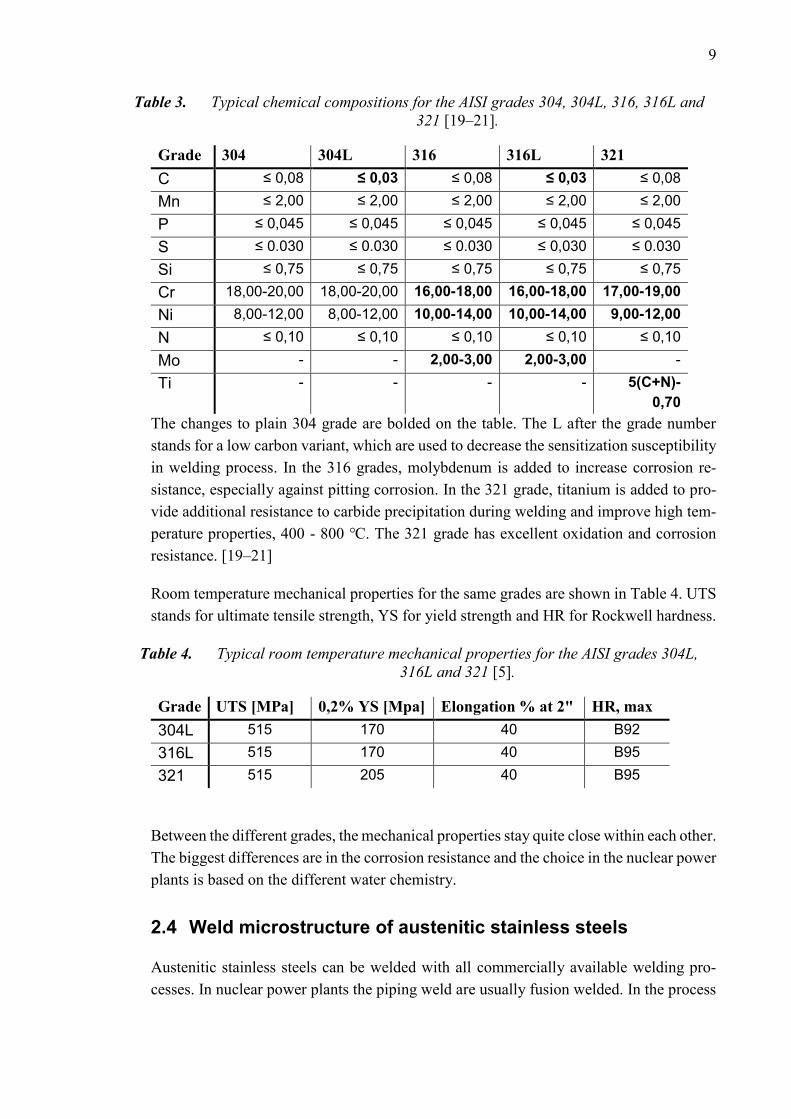
Table 3. Typical chemical compositions for the AISI grades 304, 304L, 316, 316L and
321 [19–21].
Grade 304 304L 316 316L 321
C ≤ 0,08 ≤ 0,03 ≤ 0,08 ≤ 0,03 ≤ 0,08
Mn ≤ 2,00 ≤ 2,00 ≤ 2,00 ≤ 2,00 ≤ 2,00
P ≤ 0,045 ≤ 0,045 ≤ 0,045 ≤ 0,045 ≤ 0,045
S ≤ 0.030 ≤ 0.030 ≤ 0.030 ≤ 0,030 ≤ 0.030
Si ≤ 0,75 ≤ 0,75 ≤ 0,75 ≤ 0,75 ≤ 0,75
Cr 18,00-20,00 18,00-20,00 16,00-18,00 16,00-18,00 17,00-19,00
Ni 8,00-12,00 8,00-12,00 10,00-14,00 10,00-14,00 9,00-12,00
N ≤ 0,10 ≤ 0,10 ≤ 0,10 ≤ 0,10 ≤ 0,10
Mo - - 2,00-3,00 2,00-3,00 -
Ti - - - - 5(C+N)-
0,70
The changes to plain 304 grade are bolded on the table. The L after the grade number
stands for a low carbon variant, which are used to decrease the sensitization susceptibility
in welding process. In the 316 grades, molybdenum is added to increase corrosion re-
sistance, especially against pitting corrosion. In the 321 grade, titanium is added to pro-
vide additional resistance to carbide precipitation during welding and improve high tem-
perature properties, 400 - 800 ℃. The 321 grade has excellent oxidation and corrosion
resistance. [19–21]
Room temperature mechanical properties for the same grades are shown in Table 4. UTS
stands for ultimate tensile strength, YS for yield strength and HR for Rockwell hardness.
Table 4. Typical room temperature mechanical properties for the AISI grades 304L,
316L and 321 [5].
Grade UTS [MPa] 0,2% YS [Mpa] Elongation % at 2" HR, max
304L 515 170 40 B92
316L 515 170 40 B95
321 515 205 40 B95
Between the different grades, the mechanical properties stay quite close within each other.
The biggest differences are in the corrosion resistance and the choice in the nuclear power
plants is based on the different water chemistry.
2.4 Weld microstructure of austenitic stainless steels
Austenitic stainless steels can be welded with all commercially available welding pro-
cesses. In nuclear power plants the piping weld are usually fusion welded. In the process

10
the metal parts are heated until they melt together. The process can be done with or with-
out a filler material. Generally austenitic stainless steels are considered to have good
weldability, but they have a lower heat conductivity than carbon steels and higher thermal
expansion rate which has to be taken into consideration while welding. [17]
A fusion weld can be divided into three sections, the fusion zone, heat affected zone
(HAZ) and the unaffected base metal. In the fusion zone, the actual joining happens, when
the base metal and filler melt solidify. The microstructure depends on the solidification
behavior, the shape and size of the grains, porosity, inclusions and hot cracking. In the
HAZ no melting happens but the heat input is enough to alter the grain structure via re-
crystallization and/or grain growth. [17, 22]
2.4.1 Fusion zone microstructure
In the fusion zone, four kinds of solidification behavior for austenitic stainless steels hap-
pen. The solidification types can be seen in reference to the pseudobinary phase diagram
in Figure 7. The Fe content is constant throughout the diagram but the ratio of Creq to Nieq
changes.
Figure 7. Austenitic stainless steel weld solidification types [17].
Type A, AF, FA and F. The A and AF types are primary austenite solidification, where
austenite solidifies first. In FA and F, delta (δ) ferrite is the first phase to solidify, but
solid-state transformations happen at lower temperatures, when δ ferrite is no longer sta-
ble. [15, 21] As the ratio of Creq/Nieq increases, the primary δ ferrite types FA and F take

11
over, although the solidification rate also has an effect on the final phase. In the fully
austenitic type A solidification, no ferrite is present. The solidified austenite has a sub-
structure of dendrites and cells. The substructure follows from alloying element and im-
purity segregation and it is preserved due to low elevated temperature diffusivity of the
alloying elements and impurities. Also due to the lack of ferrite, the hot cracking suscep-
tibility is higher for the type A solidified welds. In the AF type solidification some eutec-
tic ferrite is formed at the end of the solidification process, as can be seen from Figure 7.
The ferrite formation starts earlier as the Creq/Nieq ratio increases. Ferrite stabilizers, most
notably Cr and Mo, segregate to the subgrain boundaries to allow the formation of δ fer-
rite and keep it stable during weld cooling. [17, 23, 24] Type A and type AF solidification
are shown schematically in Figure 8 and metallographically in Figure 10.
Figure 8. Type AF solidification (left) type A solidification (right) [17].
Ferrite is in the form of liquid droplets at the subgrain boundaries in the AF type. In
addition, Ni segregates to the cell subgrain boundaries, but the segregated Cr concentra-
tion profiles are higher to allow δ ferrite formation. [23]

12
To prevent hot cracking of the weld metal and HAZ a minimum amount of δ ferrite is
required. The advantage of ferrite is based on its ability to dissolve more unwanted ele-
ments like sulfur and phosphorous compared to austenite. Otherwise, these elements can
form low melting liquids by microsegregation during the weld solidification and cause
cracking along the subgrain boundaries. The low melting liquid does not so easily wet
ferrite-austenite boundaries than the austenite-austenite boundaries. In addition, the
boundaries that have ferrite remain more irregular compared to the ones between austen-
ite, this creates a more complex crack path to resist cracking. Typically, it is considered
that about 5% or more δ ferrite is enough to lower the hot cracking susceptibility [25].
However, δ ferrite in small quantities provides initiation sites for pitting corrosion. The
amount of ferrite in austenitic stainless steel weldments is presented with the ferrite num-
ber, FN. FN is based on the magnetism of ferrite and it approximates the volume percent-
age accurately to around 8 FN. From the room temperature weld metal ferrite content the
solidification type also can be estimated. FN number of 0 is estimated as solidification
type A. From 0 up to 3 refers to AF type while FN between 3 and 20 refers to the FA
type. Above 20 FN the F type is presumed. [17, 23–26]
In the FA type solidification of peritectic or eutectic austenite is formed at ferrite bound-
aries at the end of solidification. After solidification, the ferrite content is around 80%
depending on the Creq/Nieq ratio but solid-state transformations during the cooling process
lower the ferrite amount gradually. Finally, the ferrite is retained as skeletal or lathy fer-
rite, shown in Figure 9. However if the ratio of Creq/Nieq is increased enough the solidifi-
cation will happen as type F where no austenite is present at solidification. [17, 27]

13
Figure 9. Type FA solidification, skeletal ferrite (left) lathy ferrite (right) [17].
Skeletal ferrite is a result of moderate cooling rate and the Creq/Nieq is low in the type FA
range (Figure 7). During cooling ferrite transforms into austenite until the ferrite sections
are enough enriched in ferrite stabilizers and depleted in austenite stabilizers. The result-
ing ferrite is stable in lower temperatures when diffusion is slower. The lathy ferrite oc-
curs on higher cooling rates and Creq/Nieq ratios. Limited diffusion time favors the shorter
distance diffusion making the laths more closely bundled than the skeletal ferrite
laths/ribs. With extremely high cooling rates, massive transformation from ferrite to aus-
tenite is also possible. The type F fully ferritic solidification is rather uncommon because
the used filler metals are selected to favor FA solidification and get FN of 5 to 20. Finally,
metallographical illustration of lathy and skeletal FA solidification is shown in Figure 10.
[17, 25, 27]

14
Figure 10. Microstructure of type FA solidification, skeletal ferrite (up left),
lathy ferrite (bottom left), type A solidification (top right) and type AF solidifica-
tion (bottom right) [17].
2.4.2 Heat affected zone (HAZ)
The heat affected zone is initially in the same state as the base material. However, the
heat can cause phenomena like grain growth, ferrite formation, precipitation and grain
boundary liquation. Significant grain growth does not usually occur when the steel is at
the hot-rolled state before welding, unless the heat input is extremely high. However, if
previous cold work has been done grain coarsening and recrystallization can soften the
HAZ considerably. [17]
Ferrite formation can also occur in the HAZ where it has beneficial effect against liqua-
tion cracking. The amount of ferrite is usually low because of limited diffusion times and
some formed ferrite can transform back to austenite upon further cooling. The Creq/Nieq
ratio determines the possibility of ferrite formation as can be seen from Figure 7. [17, 23]
The heat levels at HAZ cause precipitates of the base metal to dissolve. Upon cooling
precipitation happens again, usually along grain boundaries or austenite-ferrite phase
boundaries. Most common precipitates are carbides and nitrides. Excessive carbide pre-

15
cipitation can lead to local depletion of chromium and deterioration of corrosion re-
sistance. This phenomenon is called sensitization and it means the susceptibility to inter-
granular corrosion, illustrated in Figure 11. [17]
Figure 11. Chromium depleted zones near grain boundaries, sensitization
[28].
Sensitization can be controlled with correct weld procedure. In addition intergranular cor-
rosion also has an effect on the stress corrosion cracking, discussed in chapter 2.5.2.
2.5 Austenitic stainless steel weld flaws
2.5.1 Weld distortion
Thermal expansion coefficient for austenitic stainless steels is greater than for ferritic
stainless steels and also the thermal conductivity is low. This makes weld distortion more
common. Weld distortion happens due to uneven cooling and expansion of the weld and
adjacent base metal. Distortion can be controlled with welding process parameters: weld-
ing speed, heat input, pre- and post-heat treatments. Distortion can also be controlled with
proper joint design: weld length and thickness. In austenitic stainless steels the phase
transformations upon weld cooling also contribute to the distortion, since austenite and
ferrite have different volumes. [29]
2.5.2 Stress corrosion cracking
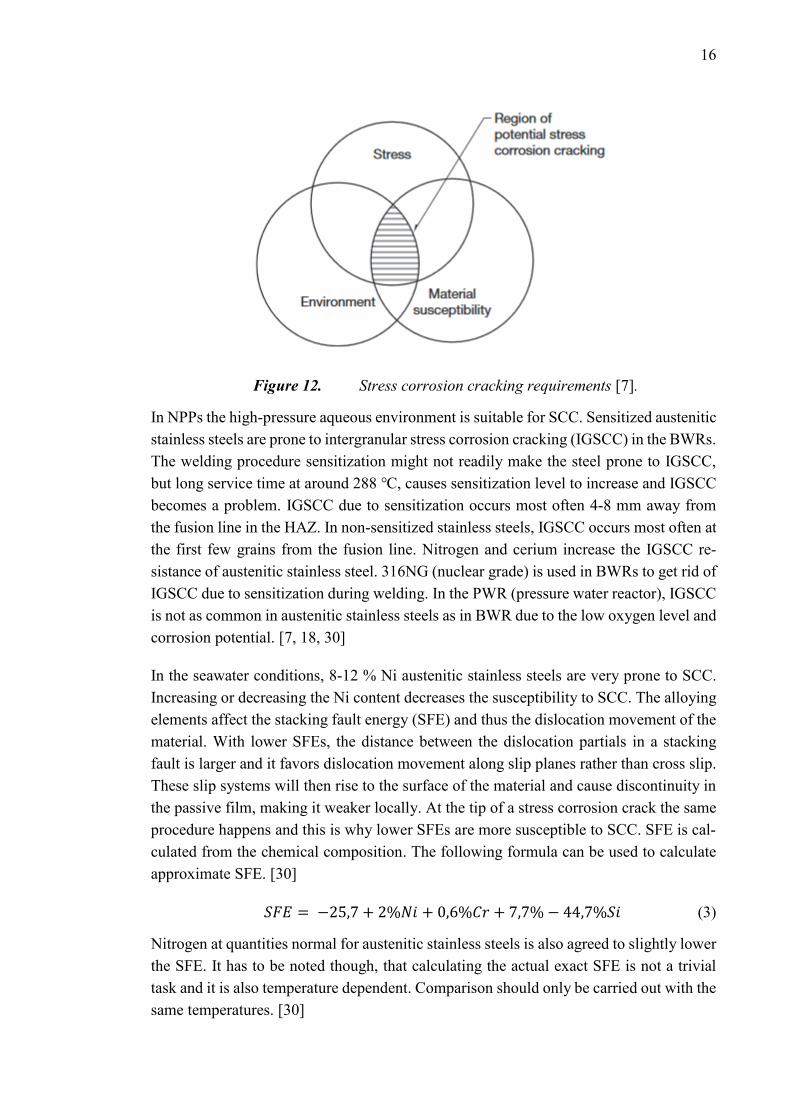
Requirements for stress corrosion cracking (SCC) are suitable material, environment and
level of stress illustrated in Figure 12.
16
Figure 12. Stress corrosion cracking requirements [7].
In NPPs the high-pressure aqueous environment is suitable for SCC. Sensitized austenitic
stainless steels are prone to intergranular stress corrosion cracking (IGSCC) in the BWRs.
The welding procedure sensitization might not readily make the steel prone to IGSCC,
but long service time at around 288 ℃, causes sensitization level to increase and IGSCC
becomes a problem. IGSCC due to sensitization occurs most often 4-8 mm away from
the fusion line in the HAZ. In non-sensitized stainless steels, IGSCC occurs most often at
the first few grains from the fusion line. Nitrogen and cerium increase the IGSCC re-
sistance of austenitic stainless steel. 316NG (nuclear grade) is used in BWRs to get rid of
IGSCC due to sensitization during welding. In the PWR (pressure water reactor), IGSCC
is not as common in austenitic stainless steels as in BWR due to the low oxygen level and
corrosion potential. [7, 18, 30]
In the seawater conditions, 8-12 % Ni austenitic stainless steels are very prone to SCC.
Increasing or decreasing the Ni content decreases the susceptibility to SCC. The alloying
elements affect the stacking fault energy (SFE) and thus the dislocation movement of the
material. With lower SFEs, the distance between the dislocation partials in a stacking
fault is larger and it favors dislocation movement along slip planes rather than cross slip.
These slip systems will then rise to the surface of the material and cause discontinuity in
the passive film, making it weaker locally. At the tip of a stress corrosion crack the same
procedure happens and this is why lower SFEs are more susceptible to SCC. SFE is cal-
culated from the chemical composition. The following formula can be used to calculate
approximate SFE. [30]
𝑆𝐹𝐸 = −25,7 + 2%𝑁𝑖 + 0,6%𝐶𝑟 + 7,7% − 44,7%𝑆𝑖 (3)
Nitrogen at quantities normal for austenitic stainless steels is also agreed to slightly lower
the SFE. It has to be noted though, that calculating the actual exact SFE is not a trivial
task and it is also temperature dependent. Comparison should only be carried out with the
same temperatures. [30]

17
Elevated temperatures increase the SCC susceptibility and it often occurs during cooling
of weldments. Different microstructures have different sensitivity to SCC. The δ ferrite
content lowers the susceptibility, because it makes the crack path more complicated. The
stresses can follow from the service conditions, residual stresses from manufacturing or
welding or fit up stresses. Heat treatments can be used to relieve the residual stresses, but
with special care to avoid sensitization. Sensitization is the most common cause of IG-
SCC, but it is also possible in non-sensitized areas. SCC can also be transgranular
(TGSCC) in austenitic stainless steels, but that is mainly due to chlorides. In NPP primary
systems it can happen due to leakage of condensation water, but the occurrence is rare.
[7, 30]
SCC resistance can be affected with different surface finish methods after welding.
Rougher surfaces have deeper grooves, which can act as initiation sites for the cracking.
However, surface grinding/machining causes heating and work hardening of the surface.
This can lead to development of residual stresses upon cooling and even phase transfor-
mation to martensite increasing the SCC susceptibility. While doing surface finishing
work care should be taken not to induce too much strain on the surface. [30]
In modern NPPs, the environmental conditions and the stresses imposed to material are
well known, thus traditional SCC does not become a problem. Instead, irradiation assisted
stress corrosion cracking (IASCC) is a phenomenon causing difficulties in the primary
circuit. The reasons behind IASCC are not fully understood, since the radiation has effects
on the water chemistry, microstructure and microchemical properties. However, the pri-
mary effects of the radiation to SCC are identified: segregation, hardening, relaxation and
radiolysis. Radiolysis is the radiation effect on the water chemistry; the effect is evaluated
by the corrosive effect to the material, and it is reasonably well known. Radiation induced
grain-boundary segregation (RIS) is local depletion (Cr) or enrichment (Ni, Si) of ele-
ments at grain boundaries. Microstructural changes occur in radiation hardening (RH),
where radiation damage creates obstacles for dislocation motion (vacancy/interstitial
loops). At some slip plane dislocations move through these obstacles and these slip planes
will become favored in further dislocation motion. Radiation creep relaxation can cause
dynamic strains when relaxing welding residual stresses and by that, increase SCC sus-
ceptibility. Swelling is a possible effect on temperatures at above 300℃ and has been
observed in PWR baffle former bolts. Precipitation and dissolution effects caused by ir-
radiation are also a possible factor on IASCC, but conclusive studies have not yet been
performed. The different effect of these phenomena to SCC are illustrated in Figure 13.
[18, 31–34]

18
Figure 13. Effect of hardness (RH) and Cr depletion (RIS) to SCC susceptibil-
ity in CP-304 SS (commercial purity) in relation to the dose [32].
Different alloying elements in different quantities, water environment, RH, RIS, thermal
segregation, individual effects of all the different phenomena are hard to evaluate. Espe-
cially since the effects do not come only due to irradiation, but from the primary fabrica-
tion, welding and joining processes as well. However, the rate and most severe combina-
tions that cause SCC can be identified. This allows SCC [31, 32, 34]
2.5.3 Weld solidification cracking
Weld solidification cracking in austenitic stainless steels is mostly affected by the com-
position. The cracking susceptibility of different solidification types can be seen in Figure
14.

19
Figure 14. Solidification cracking susceptibility in relation to different austen-
itic stainless steel solidification types and chromium to nickel equivalent ratio
[17].
The fully austenitic solidification type A is most susceptible, but with delta ferrite, in AF,
the resistance is increased. Both primary ferrite solidification types are more resistant than
the primary austenite types. Also how the welding is carried out has an effect on the so-
lidification cracking, with high travel speeds, heat inputs and large weld beads possibility
for solidification cracking increases. The ferrite formed at the solidification grain bound-
aries creates a difficult crack path, compared to type A solidification grain boundaries.
[17]
Impurities like sulfur and phosphorous increase the susceptibility to solidification crack-
ing. Ferrite has higher solubility of the impurity elements. The effect of impurities into
the solidification cracking susceptibility is clear even with very low impurity levels
(>0.002 wt% in fully austenitic). Achieving this high purity is not economically reasona-
ble and that is why the solidification behavior, to allow enough δ ferrite, has to be con-
trolled. [17, 35]
2.5.4 Liquation cracking
Liquation cracking occurs in multi-pass welds that are fully austenitic. They are also
called microcracks or microfissures as they are small in length and width and hard to
detect. Liquation cracking is best controlled with the composition to enable some ferrite
formation. If ferrite is not allowed, the heat input should be controlled and the amount of
impurities, like phosphorous and sulfur, minimized. Also, specific filler rods that have
increased amounts of manganese to limit liquation cracking in fully austenitic welds can

20
be used. Smaller grain size increases the resistance to liquation cracking. With smaller
grain size, the grain boundary area is greater and segregation is reduced. [17]
In addition to the weld metal itself liquation cracking also occurs in the HAZ right next
to the fusion zone. Liquid films form along the grain boundaries in this partially melted
zone. Same preventive actions as in weld metal are used to prevent HAZ liquation crack-
ing. [17]
2.5.5 Ductility dip cracking
Ductility dip cracking (DDC) is based on sudden elevated temperature ductility decrease
in FCC metals. The cracking occurs along migrated grain boundaries. Fully austenitic
welds are most susceptible. Best way to prevent DDC is to have some ferrite, which
makes the grain boundaries, in which the cracks propagate, more complex increasing the
cracking resistance. DDC occurs in the weld metal and HAZ. Large grain size and weld-
ments with thick sections are prone to DDC. Strain-to-fracture tests can be used to eval-
uate the DDC susceptibility. [17, 36]
Solidification and liquation cracking occur in the brittle temperature range, BTR. DDC
takes place at a lower temperature. DDC cracks can often be mistaken with liquation
cracks and it is possible that the two different cracks merge making identification harder.
Figure 15 shows the BTR temperature and the ductility dip. [17]
Figure 15. Ductility dip temperature and BTR [17].
TL is the liquidus and TS solidus temperature.

21
2.5.6 Contamination cracking
Three different types of contamination cracking are introduced in this chapter, copper
contamination cracking (CCC), zinc contamination cracking (ZCC) and helium induced
cracking. CCC occurs due to externally induced copper contamination, from used tools
or other parts. Copper as an alloying element is not a cause of CCC. The cracking happens
along austenite grain boundaries when molten copper finds its way to the grain boundary.
The melting temperature of copper is 1083 ℃. CCC can be eliminated by removing the
copper source. However, the identification of the source can prove difficult. [7, 17]
Zinc contamination cracking has a similar mechanism as CCC. It occurs when joining
galvanized stainless steel with austenitic stainless steel. Zinc has significantly lower melt-
ing temperature than copper and it boils at 906 ℃. The evaporated zinc makes its way to
the austenitic stainless steel HAZ grain boundaries, and the cracking occurs along the
grain boundaries. To avoid ZCC, zinc should be dissolved from the galvanized steel be-
fore joining. [17, 37]
Helium induced cracking can occur in NPPs. It has been observed in 304L repair welding.
Helium forms inside the steel as a product of the neutron irradiation, from B512 or Ni28
59
isotopes. Helium has low solubility in the steel so it forms as bubbles at defects and grain
boundaries. The bubbles move and grow via diffusion along the grain boundaries, until
adequate restriction that leads to cracking. The cracking is hard to avoid since helium is
formed due to the irradiation and cannot be removed. [17, 38]

22
3 ULTRASONIC INSPECTION
Ultrasound is one of the few methods that can be used to detect flaws inside of objects,
without breaking them. Ultrasonic beam is introduced to the inspected object and the am-
plitude and time it takes for the beam to reflect back or the time for it to go through is
measured. Ultrasonic inspection setups can be customized to match the requirements of
the inspected object and inspection accuracy requirements. Ultrasound can vary in fre-
quency, wavemode and different angles can be used. The process can also be automatized.
However, carrying out ultrasonic inspection requires a professional inspector with suffi-
cient qualifications. In nuclear power plants ultrasound is used mostly in in-service in-
spection of welds and thickness measurements.
In the chapters 3.1-3.5 the theory behind ultrasound and ultrasound generation is dis-
cussed alongside with some ultrasonic inspection techniques.
3.1 Ultrasound
Ultrasound is categorized as sound with a frequency of over 20 kHz and it is inaudible to
the human ear. The speed of sound propagation, v, is determined as v = λf. Where λ is the
wavelength and f is the frequency. The velocity depends on the density of the medium in
which the sound propagates and the wave type. It is calculated with the following equa-
tion, using the wave type corresponding modulus. [39]
𝑣 = √𝐶𝑖𝑗
𝜌 (4)
Where ρ is density and Cij is the elastic constant. The elastic constant varies depending
on the situation, the vibration of the material particles varies with the wave type. For
compressive waves, longitudinal modulus L is used, for shear waves, Shear modulus S is
used.
Sound velocity in air is around 330 m/s and in stainless steels around 5800 m/s. Although,
relatively large variations come with different types of stainless steels and different grain
sizes and also temperature. [39–41]
Sound (and ultrasound) propagation is oscillation of material particles. This is why sound
does not propagate in a vacuum. The propagation can happen in several different wave-
forms, like longitudinal or transverse wave, shown in Figure 16. Material is not trans-
ported by these soundwaves. [39, 42]

23
Figure 16. Longitudinal and transverse wave propagation [43].
In the Figure 16 the wave propagation happens from left to right. In longitudinal waves
or compression waves, the oscillations happen in the direction of the wave propagation
and periodically the particles are compressed close to each other and periodically rarified
away from each other. The wavelength is the length from one point to the next point
where the oscillation is at the same point. For example from one point where particles are
closely compressed to the next similar position. The amplitude of the wave is the devia-
tion of particles from their rest position, and at maximum deviation (at the compressed
points) the amplitude is maximum. How frequently (T) these points occur determines the
frequency of the sound, f=1/T. Longitudinal waves can propagate in solids, but also in
gases and liquids unlike the transverse wave, which can only propagate in solids or very
high viscosity liquids. [39, 42]
In the transverse or shear wave the oscillations happen at a right angle or transverse to the
propagation direction. The wavelength can again be determined between two points that
are at the same phase, for example at two points where the particle is at maximum devia-
tion from the rest position. At that point also the amplitude is at maximum. Because the
oscillations happen in the transverse direction the speed of transverse wave is lower than
the longitudinal wave, which results at a shorter wavelength at same frequencies. This
can be utilized in improving the resolution of inspection and allows detection of smaller
flaws. Other waveforms also exist like the Rayleigh waves and plate waves. [39]
Rayleigh or surface waves are a combination of shear and longitudinal waves. According
to the name they only travel on the surface of the solid, the penetration depth is only about
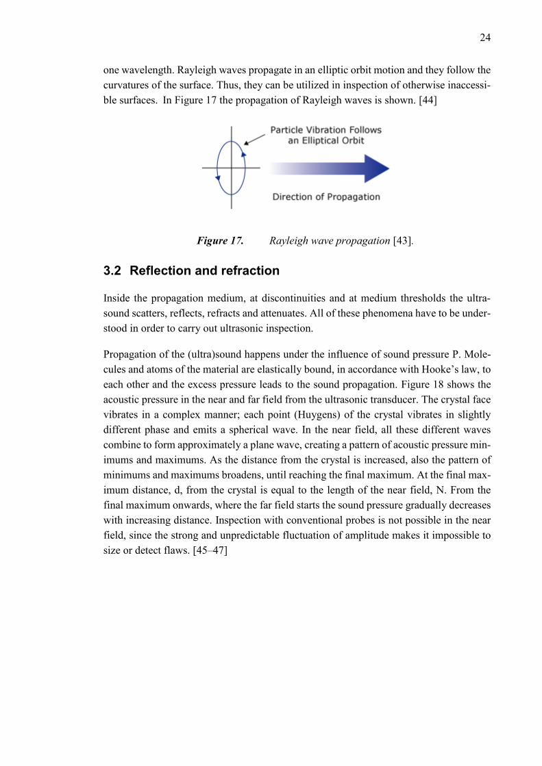
24
one wavelength. Rayleigh waves propagate in an elliptic orbit motion and they follow the
curvatures of the surface. Thus, they can be utilized in inspection of otherwise inaccessi-
ble surfaces. In Figure 17 the propagation of Rayleigh waves is shown. [44]
Figure 17. Rayleigh wave propagation [43].
3.2 Reflection and refraction
Inside the propagation medium, at discontinuities and at medium thresholds the ultra-
sound scatters, reflects, refracts and attenuates. All of these phenomena have to be under-
stood in order to carry out ultrasonic inspection.
Propagation of the (ultra)sound happens under the influence of sound pressure P. Mole-
cules and atoms of the material are elastically bound, in accordance with Hooke’s law, to
each other and the excess pressure leads to the sound propagation. Figure 18 shows the
acoustic pressure in the near and far field from the ultrasonic transducer. The crystal face
vibrates in a complex manner; each point (Huygens) of the crystal vibrates in slightly
different phase and emits a spherical wave. In the near field, all these different waves
combine to form approximately a plane wave, creating a pattern of acoustic pressure min-
imums and maximums. As the distance from the crystal is increased, also the pattern of
minimums and maximums broadens, until reaching the final maximum. At the final max-
imum distance, d, from the crystal is equal to the length of the near field, N. From the
final maximum onwards, where the far field starts the sound pressure gradually decreases
with increasing distance. Inspection with conventional probes is not possible in the near
field, since the strong and unpredictable fluctuation of amplitude makes it impossible to
size or detect flaws. [45–47]

25
Figure 18. Acoustic pressure in the near field and far field [47].
This pressure causes particles to be displaced from their rest position with the velocity Q.
Excess pressure and displacement velocity can be used to calculate the acoustic imped-
ance.
𝑍 =𝑃
𝑄 (5)
Acoustic impedance can also be expressed with density ρ and sound velocity v. [46]
𝑍 = 𝜌𝑣 (6)
The difference in acoustic impedances, the acoustic impedance mismatch, determines the
transmitted and reflected acoustic energies. With greater impedance mismatch the greater
the reflected energy is. The sum of reflected and transmitted energies is the same as the
initial energy. If the acoustic impedances of both materials are known the reflection co-
efficient R can be calculated. [46]
𝑅 = (𝑍2−𝑍1
𝑍2+𝑍1)
2
(7)
For example when considering inspection done in immersion at the threshold between
water and stainless steel only about 12% of the energy is transmitted through to the in-
spected steel block. The energy is further diminished when it reflects back from the back-
wall of the steel block and transmits through the front again towards the transducer. In
this process only 1,3% of the original energy is returned to the transducer, theoretically.
The amount is further diminished due to attenuation and scattering. Because only minimal
amount of the initial energy is returned the signal strength is enhanced by increasing gain.
This is usually calculated in the logarithmic decibel scale, in which 50 % corresponds to
approximately 6 dB, using the following equation, where P1 is the amplitude at certain
point and PR is the reference point amplitude (maximum). [46, 48, 49]
dB = 20 log (P1
PR) (8)

26
Reflection and refraction (transmit) of the sound is also dependent on the angle at which
the sound approaches the material threshold. Snell’s law is used to determine the refracted
angle at the threshold between two materials with different acoustic impedances. [46]
𝒔𝒊𝒏𝜶𝟏
𝒔𝒊𝒏𝜶𝟐=
𝒗𝟏
𝒗𝟐 (9)
in which α1 is the incident angle, α2 the refracted angle and v1 and v2 the sound velocities
of the different materials. Snell’s law is illustrated in Figure 19. [44, 46]
Figure 19. Snell’s law. [46]
The longitudinal incident wave is reflected with the same angle as the incident angle α1.
Part of the wave is also transmitted through to the other medium with a reflected angle of
α2. However, in practice this is not the full case. At the threshold the incident longitudinal
wave will also convert into a shear wave. The shear wave will reflect and refract from the
threshold but the refracted and reflected angles will be smaller, since the velocity of the
shear wave is lower than the velocity of the longitudinal wave. Snell’s law with wave
conversion is illustrated in Figure 20. [44, 46]

27
Figure 20. Waveform conversion at material threshold. [46]
β1 and β2 are the reflected and refracted angles of the shear wave. The wave conversion
is utilized in angled transducers. Understanding the ultrasound interactions inside the ma-
terial is considerably easier if only one waveform is present. Critical angles are utilized
in this. The first critical angle is the incident angle at which the refracted angle for the
longitudinal wave α2 is 90°. At this angle only the shear wave is transmitted into the
second medium, the longitudinal component is fully reflected. At the second critical angle
both the longitudinal and shear components are reflected and neither penetrates into the
second medium. This is utilized in generation of Rayleigh or surface waves. [46]
3.3 Attenuation
Different attenuation phenomena affect the strength of the received signal. With distance
from the transducer the sound attenuates due to absorption, scattering, diffraction and
beam spreading. [47]
In monocrystalline materials absorption is the main attenuation factor. Ultrasonic energy
is converted to heat via thermal conductivity and internal friction. The wave motion heats
the substance as it is compressed and cools it as it rarifies. The energy is lost as the heat
flows slower than the ultrasound wave. Absorption can be accounted for by increasing
gain on the ultrasonic device. In polycrystalline materials absorption occurs: heat flows
away from the grains that have been subject to more compression or expansion than the
surrounding grains. However, for polycrystalline materials scattering is the main contrib-
uting factor to attenuation. [47, 50]
28
Scattering happens at material discontinuities, like grain and twin boundaries and inclu-
sions. At said discontinuities energy of the main beam is scattered, but scattering cannot
be eliminated by increasing the gain, because the scattered waves return to the transducer
as noise and this would only result in increasing the noise levels. This is an elementary
problem in inspection materials with anisotropy like austenitic stainless steel welds. Also
at the crystal boundaries and boundaries between different phases, mode conversion hap-
pens, due to the differences in the velocity of ultrasound and acoustic impedances. Scat-
tering of the sound mainly depends on the grain size and wavelength of the ultrasound. If
the wavelength is less than 0.01 times the grain size then scattering is negligible, but if
the number is 0.1 or higher scattering can make inspection impossible. The problem with
higher wavelength in turn means that smaller flaws can be missed during inspection; this
can be counteracted by using shear waves that propagate with a lower velocity resulting
in lower wavelengths at the same frequencies. [47, 50]
Diffraction of the sound beam occurs at the edges of reflecting surfaces and at small flaws
like pores or inclusions the sound wave bend from the original pattern. The initial propa-
gating wave consists of parallel planes that all oscillate in the same phase. When the sound
diffracts, behind the edge or inclusion parts of the soundwave go through a change in
phase. This leads to different interference. The interference can be constructive or de-
structive. In destructive interference, the other plane is half period out of phase and can-
cels out the sound. This can lead to dead zones in the inspection and can leave flaws
unregistered. In constructive interference, two waves are in the same phase and are added
to each other, increasing the amplitude. [47, 51]
Acoustic pressure of the ultrasonic beam decreases in the far field of the ultrasonic beam.
The beam wave front spreads as the distance from the source increases. The total attenu-
ation in a material with attenuation coefficient α and length L can be calculated as: [45]
𝑃 = 𝑃0𝑒(−𝛼𝐿) (10)
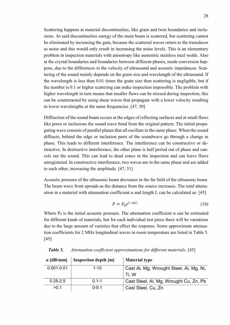
Where P0 is the initial acoustic pressure. The attenuation coefficient α can be estimated
for different kinds of materials, but for each individual test piece there will be variations
due to the large amount of varieties that effect the response. Some approximate attenua-
tion coefficients for 2 MHz longitudinal waves in room temperature are listed in Table 5.
[45]
Table 5. Attenuation coefficient approximations for different materials. [45]
α [dB/mm] Inspection depth [m] Material type
0.001-0.01 1-10 Cast Al, Mg; Wrought Steel, Al, Mg, Ni,
Ti, W
0.25-2.5 0.1-1 Cast Steel, Al, Mg, Wrought Cu, Zn, Pb
>0.1 0-0.1 Cast Steel, Cu, Zn

29
Anisotropic materials, such as austenitic welds, distort the sound waves. This occurs be-
cause of difference in the direction of sound wave propagation and energy transfer.
Snell’s law can no longer be directly utilized and the exact location of the sound wave is
harder to predict. The attenuation is greater and flaws become harder to detect (and lo-
cate). [50]
3.4 Ultrasound generation
Ultrasound can be generated with piezoelectricity, electromagnetic (EMAT), laser gener-
ation, magnetostriction and electrostriction. Of these methods, piezoelectricity is most
widely used and it is also used in the measurements done in this thesis. [44]
Piezoelectric crystals operate via the direct and inverse piezoelectric effect. In the direct
effect stress applied to a crystal produces a potential difference between the opposing
sides of the crystal (in addition to strain). The direct effect is utilized in detecting the
ultrasonic waves. in the inverse effect applying a potential difference to different sides
also induces a strain, this is used in the generation of ultrasound. The piezoelectric effect
works with high frequencies (up to 10 THz). [39, 44]
The piezoelectric effect requires a lack of center symmetry in the crystals. For example if
in the case of a quartz piezoelectric crystal is placed between two metal plates that are
capable of imbuing stress and acting as electrodes. When no stress is applied via the plates
the center of the positive and negative charges is the same, but when stresses are applied,
compressive or tensile, the charges distribute asymmetrically, which leads to different
center of gravities for the negative and positive charges. As a result the electrodes accu-
mulate different charges and a potential difference is generated. [44]
Different piezoelectric materials are listed in Table 6 with reference to their preferred
applications.

30
Table 6. Piezoelectric material applications and characteristics [52].
Coup-
ling
Inspection
mode
Piezoelectric
element
Trans-
mit
Re-
ceive
to
wa-
ter
to
me-
tal
High
tempe-
rature
use
Dam-
ping
Straight
beam
Angle
beam
Immer-
sion
Quartz P G G F G F G F G
Lithium sul-fate F E E P P E P F E
Barium ti-tanate G P G G P P G G F
Lead zirco-nate titanate E F F E E F E E F
Lead meta-niobate G F G E E E E E G P=poor F=fair G=good E=excellent
The first piezoelectric crystals were all quartz crystals, which are very durable. However
the properties highly depend on which direction the crystal is cut and the electromechan-
ical coupling factor, which refers to how efficiently electric voltage is converted to me-
chanical displacement and vice versa, is low. [52]
The target of the inspection dictates the required properties for the transducer. Active area
of the element, characteristic frequency and frequency bandwidth for the transducer ma-
terial and the type of the probe (dual element, angular, normal, immersion). The active
area of the element directly effects to the ultrasound energy that is being transmitted to
the material and the beam divergence. With larger elements the penetration depth is
greater. The characteristic frequency of a transducer element is the frequency at which is
best receives and transmits ultrasound. It is defined by the element thickness and material,
reducing the thickness increases the frequency. The transducer functions efficiently at a
band around the characteristic central frequency. The size of the band is determined as
bandwidth and it is the difference of the central frequency and lower frequencies. Usually
bandwidth is given as bandwidth at -6 dB, which refers to the bandwidth at 50 % of the
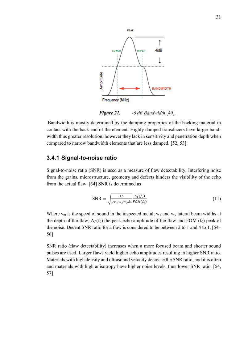
central frequency. This is illustrated in Figure 21. [52, 53]
31
Figure 21. -6 dB Bandwidth [49].
Bandwidth is mostly determined by the damping properties of the backing material in
contact with the back end of the element. Highly damped transducers have larger band-
width thus greater resolution, however they lack in sensitivity and penetration depth when
compared to narrow bandwidth elements that are less damped. [52, 53]
3.4.1 Signal-to-noise ratio
Signal-to-noise ratio (SNR) is used as a measure of flaw detectability. Interfering noise
from the grains, microstructure, geometry and defects hinders the visibility of the echo
from the actual flaw. [54] SNR is determined as
SNR = √16
𝜌𝑣𝑚𝑤𝑥𝑤𝑦∆𝑡
𝐴𝑓(𝑓0)
𝐹𝑂𝑀(𝑓0) (11)
Where vm is the speed of sound in the inspected metal, wx and wy lateral beam widths at
the depth of the flaw, Af (f0) the peak echo amplitude of the flaw and FOM (f0) peak of
the noise. Decent SNR ratio for a flaw is considered to be between 2 to 1 and 4 to 1. [54–
56]
SNR ratio (flaw detectability) increases when a more focused beam and shorter sound
pulses are used. Larger flaws yield higher echo amplitudes resulting in higher SNR ratio.
Materials with high density and ultrasound velocity decrease the SNR ratio, and it is often
and materials with high anisotropy have higher noise levels, thus lower SNR ratio. [54,
57]
32
3.5 Ultrasonic inspection techniques
3.5.1 Pulse-echo method
The pulse-echo system normally consists of a transducer, an electronic clock, an elec-
tronic signal generator/pulser, a signal amplifier and a display device. Ultrasonic energy
pulses are introduced to the inspected object at regular time intervals. Then at surfaces or
boundaries with acoustic impedance differences, the energy is reflected and/or refracted.
The reflected energy is dependent on the size and orientation of the reflector. The elapsed
time from the emitted pulse to the received pulse and the received signal energy are meas-
ured and when the velocity of ultrasound in the material is known the source of the echo
can be located. [58]
It is also possible to use a different transmitting and receiving transducers. The transduc-
ers can be still located inside the same housing or for example at either side of the in-
spected object. In the case of separate transmitting and receiving transducers the method
is called pitch and catch. [58]
Pulse-echo inspection with single element transducers is also referred to as conventional
ultrasound inspection. The inspection data is usually readily shown in the screen of the
conventional ultrasonic testing device as A-scan. In the A-scan amplitude is plot against
time. The data can also be displayed as B-scans. In a B-scan the horizontal axis refers to
the transducers position along the line which it is moved. The vertical axis shows the time
it takes for the pulse to reflect back. B-scan is a cross section of the inspected object. C-
scans are basically an image from “above” the specimen. Areas with flaws will show
higher amplitude responses and stand out from the data. B- and C-scans need the loca-
tional information of the amplitude. A, B, and C -scans can be seen in Figure 22. [58]

33
Figure 22. Formation of A, B and C -scans, IP is the initial pulse generated by
the transducer and BW is the back wall echo [59].
Weld inspection from directly above the weld is usually not possible because of the weld
crown. Probes that send sound beam directly below them are called normal probes or 0°
probes. Welds are inspected with angled transducers, that send the sound beam at a set
angle, like 45°, 60° or 70°. Weld inspection utilizes the full and half skip methods. Usu-
ally the minimum distance that has to be covered is the distance between the half and full
skip locations. In the half skip method the angled beam hits directly the weld root and in
the full skip method the sound beam first reflects off the back wall and then hits the further
fusion. Different skip distances are shown in Figure 23. [60]

34
Figure 23. Probe position and sound path at different distances [60].
Echoes from the reflectors have a higher amplitude when the sound beam hits them at
90°. Depending on the root angle of the weld the probe angle can be selected to allow
this. The half skip method is used to inspect the fusion line from the opposing side of the
weld compared to the probe location and the full skip method for the same side fusion
line as the probe. Even though the welds can’t be inspected with normal probes, the in-
spected weld area should be checked with a normal probe for possible laminations that
can’t be seen with an angle probe, but can leave dead zones and falsify the results. [60]
3.5.2 Phased array (PAUT)
In the phased array ultrasonic testing the transducer consists of multiple piezoelectric el-
ements, most commonly 16-128 elements. These elements can be separately activated to
transmit or receive. Sequencing the transmission of the ultrasonic waves from each ele-
ment combine together to from a pulse at the wanted angle, according to Huygens prin-
ciple. Each point of a wave acts as a source for a spherical wave, these waves combine to
create a wavefront [61]. The control of the different elements in the phased array trans-
ducer is done with focal laws. The focal laws determine at which point each element
transmits steering the soundwave into desired angle and focus depth. With 2D matrix
transducers the sound can also be sent at skew and tilt angles. In comparison to the con-
ventional method, this allows multiple angles to be scanned with one probe, limiting the
amount of required probes and saving time. However, the amount of data collected is
considerably larger and has to be noted in the use of PAUT. In Figure 24 the element
delays determined by focal laws are used to focus and direct the soundwaves. [62]

35
Figure 24. Focal laws used to set element delays to direct (left) and focus
(right) the sound beam [63].
With increased amount of elements the steering and focusing are more accurate, but
higher element count is needed to cover the same area, which makes the transducer more
expensive. Focusing is also only possible in the near field. The length of the near field is
calculated with equation 11, where D is the is the total aperture, element diameter times
the number of elements. [64]
𝑁𝐹𝐿 =𝐷2
4𝜆 (12)
For the instrument software the schematic of the transducer is inserted to enable the gen-
eration of desired beam. This can be seen in Figure 25. [64, 65]
Figure 25. Phased array probe dimensional parameters [65].

36
This schematic is for a transducer where the elements are on a linear spacing. A is the
total aperture in the active direction or steering direction. The opposite direction is the
passive plane, in which H is the element height. Element width e, active element spacing
g and pitch p between two elements (center-to-center) [65]. By controlling these param-
eters the characteristics of the beam are changed. As mentioned smaller element size al-
lows for more accurate steering, in commercial probes the minimum size is usually
around 0,2 mm. However, the frequency must be set to that the wavelength is higher than
the element size, otherwise side lobes will be generated in the signal. There also needs to
be enough elements to cover the whole aperture, while keeping the pitch low. Low pitch
with large aperture allows for good steering and focusing capabilities. Between these fac-
tors, cost and complexity a compromise has to be found when manufacturing the probe.
[66]
The maximum possible steering angle can be calculated with element width e and wave-
length in the inspected material by the following equation.
𝑠𝑖𝑛𝜃𝑠𝑡 = 0,514𝜆
𝑒 (13)
The sine of the maximum steering angle θst is calculated with wavelength λ and element
width e. [67] The same effect is illustrated in Figure 26.
Figure 26. Element size effect on the steering angle [67].
When the amount of elements is kept the same decreasing the element size increases the
steering angle. But the overall aperture is decreased which leads to restricted area of cov-
erage, sensitivity and focusing ability. [67]

37
4 FLAW PROPERTIES AFFECTING ULTRASONIC
DETECTION
4.1 Surface roughness and crack orientation
Crack-like defects that occur naturally are not planar and have surface roughness. The
surface roughness of a crack leads to decreased amplitude when inspection is done per-
pendicular to the crack. The surface roughness reflects the incoming beam into multiple
directions as opposed to a planar surface. This is shown in Figure 27. [68, 69]
Figure 27. Amplitude distributions of scattered waves at increasing surface
roughness (σ), using 2 MHz monochromatic wave. [68]

38
In the first case, a, the surface is very smooth and the reflection occurs strongly at 30°,
the waves interfere to form a coherent field. When increasing the surface roughness, b,
the constructive interference is weaker and at very high surface roughness, c, there is no
considerable summation in the 30° direction anymore. Instead the incident wave is scat-
tered around to a diffuse field. Increasing surface roughness of the crack-like defect [68,
70]
The effect of surface roughness is pronounced at flaw tilt angles. When the sound beam
hits the surface of the crack-like defect and the misorientation (tilt) of the defect is high
enough surfaces with higher roughness come easier to detect than smooth surfaces. This
is shown in Figure 28. [68]
Figure 28. Signal response levels of flaws with rough and smooth surfaces
with different misorientation angles [71].

39
The inspected flaws in the figure are 25 mm circular defects. It can be seen that at around
20 degrees misorientation the rough defects become easier to detect. Although, it has to
be noted that in the case of smooth or rough defects the overall received signal is dimin-
ishes as the flaw is tilted. Only the magnitude of the amplitude drop is much smaller with
the rough flaws and at some point, it will overcome the detectability of a smooth planar
defect. The level of misorientation required to see the enhanced detectability for rough
flaws depends on the size of the flaw. Larger flaws require less misorientation than
smaller ones. The effect of surface roughness can be used to separate smooth and rough
planar flaws and volumetric flaws while conducting the inspection. [68, 70]
For the sizing of the flaw, in smooth planar flaws there is a clear amplitude drop at the
edges of the flaw. In the case of rough flaws the drop is not as pinpointed, so a response
drop in the signal is difficult to measure. This can be seen in Figure 29. [68]
Figure 29. Amplitude drop observed at the edges of a smooth flaw is not no-
ticeable for rough flaws [68].
4.2 Crack opening and residual stresses
The effect of crack opening to the detectability of the crack is principally simple. Larger
crack opening yields higher amplitude response than a tight crack. The effect is based on
the vibration movement that is allowed for the surface of the crack. If the whole crack is
open, the whole crack will be allowed to vibrate and up to a saturation point the increase
in crack opening will increase the acquired signal. With partially closed or fully closed
cracks, the vibration of the reflecting surface is hindered and the response is lower. The
signal still does not fully disappear, but it is considered to be acoustically closed when
the amplitude response drops significantly. The surface roughness of the crack also af-
fects the detectability via the crack opening, smooth cracks can be acoustically more
closed than rough cracks. Also, planar cracks are acoustically more easily closed than
non-planar cracks. [68, 72]

40
For mechanical fatigue cracks the amplitude response has been shown to be different for
cold-worked and annealed specimens. For annealed material, when applying compressive
loads to close the crack, the amplitude response height drop happens fast. The annealed
specimen does not have residual stresses around the crack and the closing of the crack
happens simultaneously at whole crack length. In cold-worked specimens the crack closes
first at the crack tip and after that the whole crack gradually closes. In the amplitude
response the height decrease is first slow as the crack tip closes and then faster as the rest
of the crack closes. The difference is due to the residual compressive stresses in the cold-
worked specimens. The total amplitude drop, at yield strength of the material, is also
higher for cold-worked specimens than for the annealed specimens. [73]
Tensile residual stresses make the cracks easier to notice as they make the crack openings
larger. Compressive stresses close the crack making detection harder. In the situation of
power plant shutdown and then made in-service inspection the stress states will be static.
However, several cyclic loadings and unloadings change the amplitude height plateau.
With initial tension the plateau remains unchanged, but if followed by sufficiently high
compressive load the plateau height drops. Further loading and unloading cycles return
to the same plateau value, but less strength is required. The area around the crack goes
through plastic deformation on the first loading cycle resulting in a lower force require-
ment at subsequent loadings. The effect of cyclic loading and unloading is also shown in
Figure 30. [68, 73]

41
Figure 30. Effect of stress state on ultrasonic echo amplitude height in AISI304
for a thermal fatigue crack [73].
The effect of cyclic loading and unloading to the ultrasound amplitude is different with
thermal fatigue cracks and mechanical fatigue cracks. For thermal fatigue cracks, the am-
plitude response is lower even without external loads. The effects of external loads is also
more pronounced since the thermal fatigue cracks are readily more closed and peaks of
the crack surface roughness can be in contact with the opposing side. When the thermal
fatigue cracks are filled with water, it further restricts their detectability and regardless of
any (realistic) stress states, the cracks can be undetectable. [73]
The effect of compressive stress on a flaw varies with different probe tilt angles. This is
shown in Figure 31, where a round flaw with depth of 60 mm and diameter of 4 mm is
scanned parallel (0°), perpendicular (90°) and at 30° to the scanning surface.

42
Figure 31. Ultrasonic echo amplitude signal with different compressive loads
and probe tilt angles. (- - - -) 200 MPa; (-·-·-·-) 50 MPa; (—) unloaded, a) 0°
tilt; b) 90° tilt; c) 30° tilt [68].
In the Figure 31 a) the amplitude drops gradually to the level of 200 MPa and at 50 MPa
only slight decrease is detected. In the Figure 31 b) the drop of echo height is significant
already at 50 MPa compressive load, and in the case of Figure 31 c) the echo height drop
is more even. [68]
4.3 Oxide film
The crack can be filled with air, but also with and oxide layer and/or water. These differ-
ent surfaces of the crack or crack fills have different acoustic impedances and will effect
the behavior of the ultrasound. Presence of oxide film has been noticed to lower the de-
tectability of a crack. Closed cracks provide the amplitude drop earlier when filled with
water than when filled with air. [73, 74] However, the results are not completely conclu-
sive and it has also been reported that an oxide layer lessens the echo heights when closing
the crack. Compressive stresses on the crack surfaces should not reduce the detectability
of the crack at in service inspection. When sizing the flaw the oxide film separates the
metallic crack surfaces. The ultrasound has to pass the oxide layer with different imped-
ance altering the response as opposed to oxide free crack. [72]

43
5 RESEARCH METHODOLOGY
5.1 Ultrasound equipment
The ultrasound inspection was carried out with ZETEC DYNARAY-64/64PR-LITE flaw
detector. The detector was linked into a PC for data acquisition, which was done using
Ultravision 3,8R30 software. The probe was attached to a scanning acoustic microscope
(SAM), which can move in x and y directions with resolution up to 0.01 mm. In Figure
32 the probe attached to the SAM is shown.
Figure 32. Scanning setup for the ultrasonic inspection
The used probe system was a dual matrix probe with two 1,5 MHz probes with 5x3 ele-
ments each. However, from the probe calibration data the centre frequency was 1,8 MHz,
also used in the simulations. The probe specifications are listed in Table 7.

44
Table 7. Dual matrix probe parameters
1,5M5x3E17,5-9 E102/E106
Central Frequency (-6dB) 1,8 MHz
Bandwidth (-6dB) 57 %
Elementary pitch in axis1 3,5 mm
Elementary pitch in axis2 3 mm
Element dimensions 3,35 x 2,85 mm2
Inter-element 0,15 mm
Active area 17,35 x 8,85 mm2
The shear wave velocity was set to 3150 m/s and the longitudinal velocity at 5770 m/s.
For the plate, the used wedge was ADUX576A. Water was used as a couplant and the
plate was scanned so that it was constantly under waterbed to assure proper coupling. The
scans were conducted using 45° angle. Only one angle of the phased array probe was
utilized to allow for lower simulation times.
5.2 CIVA simulation software
CIVA is a software platform for non-destructive testing, based on the research made by
the CEA and its partners in the field of NDT simulation. It comprises of different pack-
ages for different NDT methods, like ultrasound, eddy current and radiography. The ul-
trasound module was used in this thesis and there is also a finite element module, Athena
for finite element simulation of ultrasound. Computational simulations are based on math-
ematical models that are validated with experimentation and modelling benchmark exer-
cises. Ray paths, response from the flaws, ultrasonic field computation can be simulated
with different materials. As inputs the simulations require the structure of the inspected
material, type, position and characteristics of the transducer, the computing area, wave
propagation modes and elastodynamic quantities that constitute the field (displacement).
[75, 76]
The ray tracing of CIVA is based on the model of pencil propagation. The rays originate
from one point of a transducer imitating the tip of a pencil and propagate in a cone like
shape. These rays are four component pencil vectors, but do not count attenuation, which
is applied later as a divergence factor. This method allows the simulation of complex
systems and transducers. Propagation in isotropic or anisotropic medium apply their own
slowness matrices altering the pencil vectors. The pencil is also modified at a reflection
or refraction at an interface, having their own interaction coefficients. Distortions are
made with the interaction coefficients. [75]
The flaw interactions of the incident wave are calculated with either the Kirchhoff model,
geometrical theory of diffraction (GTD) or separation of variables (SOV). The Kirchhoff

45
model is suitable for crack-like flaws and volumetric cavities. GTD is used to simulate
tip diffraction echoes from crack-like flaws and is suitable for time of flight simulations.
The SOV model is used for the simulation of scattering from cylindrical holes. [75]
5.2.1 CIVA software settings
Structural noise and attenuation were not added to the simulation to minimize simulation
times. For the calculation of sound beam interactions Kirchhoff & GTD model from
CIVA was used, which is designed for crack-like flaws [75]. A dual matrix probe with
the same properties as in the actual measurement was used, the properties are shown in
Table 7. The delay laws from the CIVA calculator were used. For the weld a CIVA stiff-
ness matrix for parametric anisotropic orientation was used.
5.3 Ultrasound data post-processing
The ultrasound data was post-processed using MATLAB. From the raw data an A-scan
line was made with the peak responses. This scan line was also converted to show decibel
responses of the amplitude using equation 7. The data from the simulation and the actual
measurement was then plot into figures. From the simulations also B-scan figures were
made.
5.4 Test piece, plate
The test piece was two rolled AISI316L plates welded together with a butt weld by MAG
welding. The weld root and crown were ground off so the test piece had an even thickness.
Test piece parameters are shown in Table 8.
Table 8. Test plate parameters
Test plate
Width [mm] 200
Length [mm] 299
Thickness [mm] 22,1
Weld
Width at top [mm] 26
Groove [°] V 60°
The flaws were made with EDM machining and numbered from one to five. The positions
of the flaws and the parameters of the test piece are shown in Figure 33 and the flaw
numbers positions and sizes are listed in Table 9.

46
Figure 33. Test plate parameters and flaw locations from the side of the EDM
notch openings.
Table 9. Flaw parameters and positions.
Width [mm] Height [mm] Position X [mm] Position Y [mm]
Flaw 5 15,0 5,3 225,00 30,00
Flaw 1 15,0 5,0 149,25 155,00
Flaw 2 15,0 5,0 146,00 100,00
Flaw 3 15,0 5,0 148.50 65,00
Flaw 4 15,0 5,0 150,00 30,00
In addition to the EDM notches (Flaws 1-5) there is an unintended surface flaw, flaw S.
However, when the plate was scanned for unintended flaws before machining the EDM
notches it could not be detected with ultrasound and is considered to be inconsequential
for the measurements. The letters a and b are used to refer to the side from which the
scans are made. In Figure 34 the test plate is shown from the side of EDM notch openings.

47
Figure 34. Test plate and the EDM notches.
5.5 Setup for flaw 5
The initial scan to test the correspondence of CIVA simulation and the actual measure-
ment was done with the flaw 5. The flaw was only scanned from one side since it is
surrounded by the base material from both sides and the results can be assumed to be
identical, also the CIVA simulation was done from one side only. The peak response at
45° scan angle was set to 80 %. Then the probe system was moved 20 mm away from the
flaw (-x direction) and 20 mm to the side (-y direction). The scanning was done in the
direction of the flaw length in 40 mm scans. The increment between the 40 mm scans was
0,5 mm steps so the total scanned area was 40 x 40 mm. The used resolution was 0.5 mm
to allow approximately 1 mm flaws to be detected. Then the same procedure was carried
out but the probe was turned 10° to each side from the perpendicular direction. This is
illustrated in Figure 35.
Figure 35. Scanning setup and probe tilt angles for flaw 5

48
In the picture the arrow points the side from which the flaw (red line) was scanned, the
flaw is at the bottom of the plate. The scanning was done at 0°, +10° and -10° angles
against the length of the flaw. The tilting was done, since the flaws in the test plate are in
the same direction as the weld, but this is not necessarily the case with real flaws, also the
probe can be misaligned with the weld in an in-service inspection.
The same setup was made in the CIVA software, which is illustrated in Figure 36.
Figure 36. Scan plan for flaw 5 at -10°.
For the ultrasound and simulation data sets, A-lines with maximum amplitude responses
were made and plot into figures represented in the results.
5.6 Setup for plate weld, flaws 1-4
The ultrasound scanning for the flaws 1-4 in the weld and HAZ were carried out in the
same way as for the scan for flaw 5. The peak response was set to 80% and from that
position the probe was moved 20 mm in -x and 20 mm in -y directions. Then the scanning
was again done with 40 mm scans and 80 0,5 mm increments to reach scanning area of
40 x 40 mm, with 0.5 mm resolution.
The same setups were also made in the CIVA software. The probe position was set 20
mm away from the flaw centre. The scan line was the same for all the probe tilt angles.
This means that in the results of -10° and +10° scans the flaw is not in the centre when

49
the probe is at 20 mm position, so the scan line corresponds to the probe position, not to
the flaw position. Also, only one scan line was selected, at a distance that the line of the
scanning would hit the bottom of the flaw. The probe was moved forward and backward
according to the exact X position of the flaw so that the distance from the probe to the
flaw is the same in each simulation. The scanning procedure is illustrated in Figure 37.
Figure 37. Scanning line for flaw 2 at +10° probe tilt.
The rough flaws were made using a Matlab algorithm to have a surface roughness
RA=0.2725 mm, consisting of 239 triangular elements representing a semi-elliptical flaw
with the same size as in the test specimen. An example of a rough flaw is shown in Figure
38. The surface roughness was selected to estimate roughness of a real EDM notch [77].
Figure 38. Rough flaw for the simulation
50
5.7 Signal-to-noise ratio
For the calculations of signal-to-noise ratio (SNR) a simplified version of equation 10
was used:
SNR =Af
An (13)
In which Af is the maximum amplitude response from the flaw and An is the average noise
level, both selected individually from each scan, since the anisotropy of the weld changes
the noise levels for each position and flaw tilt angles.

51
6 RESULTS & DISCUSSION
In this chapter, the results of the measurements and CIVA simulations are plot into fig-
ures. The flaw 5 was done as a calibration and a proof of concept measurement as the
flaw is located outside of the weld. In the figures the actual measurement is as blue (UV),
the CIVA simulation as orange, and the CIVA simulation with surface roughness (CI-
VAR) with yellow. The results of the actual measurements were fitted to match the max-
imums to the maximums of the CIVA simulations in the scan axis. The CIVA simulation
results are as simulated, since the probe is always positioned at the exact same place in
the case of rough flaws and smooth flaws. The scan axis always refers to the position of
the probe, so especially at the tilted cases the response at 20 mm scan does not come from
the middle of the flaw. In addition, a line at -6 dB is shown to clarify the sizing of the
flaws according to Characterization and sizing of discontinuities (ISO 16827:2012). In
this case, as it is known that there is only one flaw, the size is considered the area in
between the first and last point where the acquired echo surpasses the -6 dB limit. In
reality identifying the size is more difficult, since the assessment has to be made in be-
tween several clustered flaws or one flaw, according to Characterization and sizing of
discontinuities (ISO 16827:2012).
Sources of error from the measurement setup apply for all of the flaws. The scanning was
done as a raster type scan and as the mount of the probe was not completely rigid, it can
cause variation to the tilt angle of the probe. In addition, the initial setup to the tilt angles
can have error. There can be variation in the dimensions of the flaws as well.
In appendix A results for flaws 1-5 plot into same figures, with two different amplitude
axes are shown so the shape of the whole amplitude curve can be seen. In appendix B B-
scans of the simulated flaws 1-4 are shown to illustrate how the flaw size is observed.
6.1 Results for flaw 5
The data acquired from the CIVA simulation and the carried out measurement for the
flaw 5 is presented in Figure 39, Figure 40 and Figure 41. The amplitude in the CIVA
simulation does not have a noise level or attenuation set so outside of the flaw the actual
amplitude is -infinite. The CIVA simulation results are shown as orange and the carried
out measurement as blue.

52
Figure 39. Simulation versus measurement for flaw 5 at 0°.
The shape of the curve for the simulated and measured responses are very similar. The
flaw size in reality is most likely not exactly the measured dimensions and this causes
difference. The overall noise level in the carried out measurement is around -22 dB from
the maximum response and in the CIVA simulation there is no noise level. If -6 dB is
considered the line, where the flaw ends the size of the flaw is slightly smaller in the
simulation.

53
Figure 40. Simulation versus measurement for flaw 5 at -10°.
When the probe is turned -10° from the flaw length (according to Figure 35) the measured
signal comes from a smaller area than in the case of CIVA simulation at -6 dB. The overall
noise level for the measured signal is around -20 dB from the maximum response. The
difference for the CIVA simulation and the actual measurement here that should be con-
sidered is that the flaw 5 in reality is certainly not smooth. The surface of the flaw will
have texture of some kind. In addition, the dimensions can have variation.
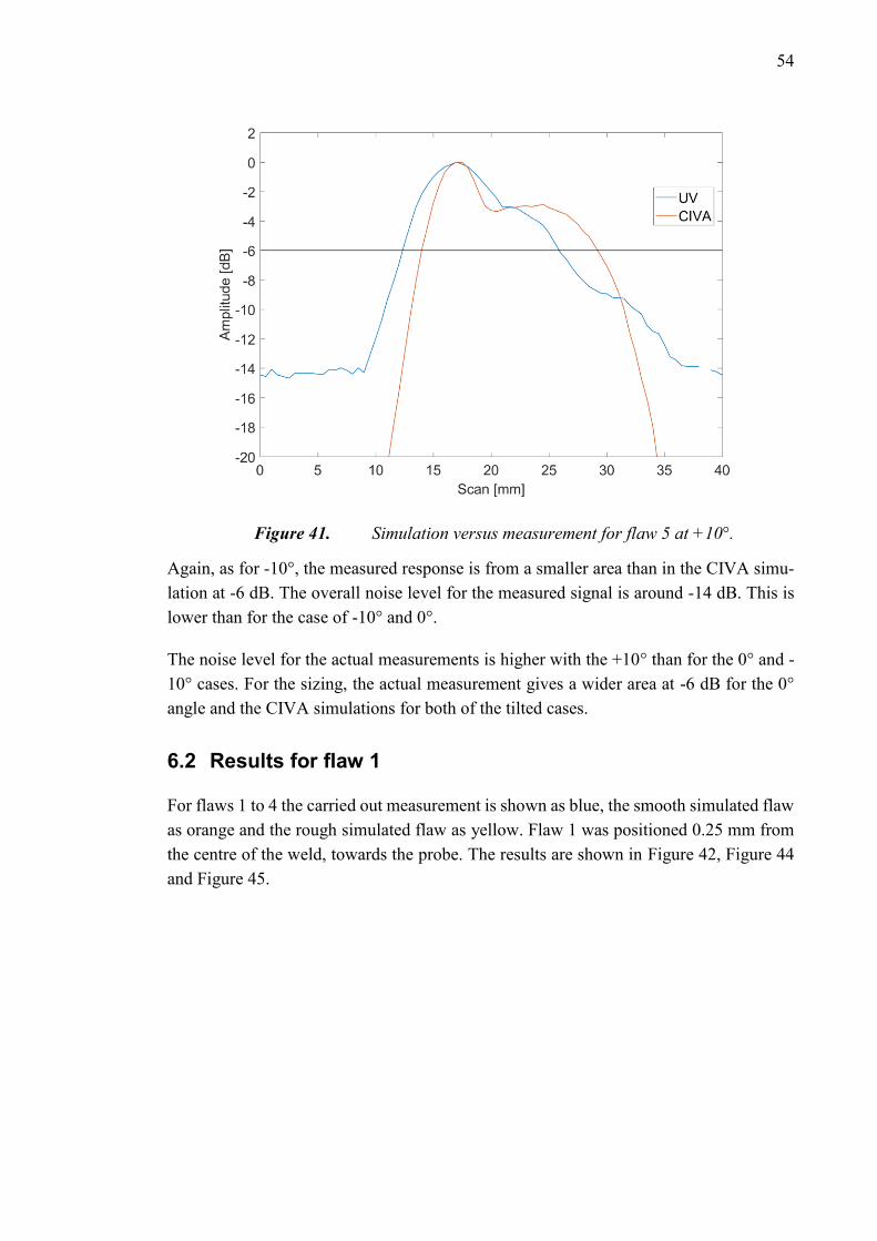
54
Figure 41. Simulation versus measurement for flaw 5 at +10°.
Again, as for -10°, the measured response is from a smaller area than in the CIVA simu-
lation at -6 dB. The overall noise level for the measured signal is around -14 dB. This is
lower than for the case of -10° and 0°.
The noise level for the actual measurements is higher with the +10° than for the 0° and -
10° cases. For the sizing, the actual measurement gives a wider area at -6 dB for the 0°
angle and the CIVA simulations for both of the tilted cases.
6.2 Results for flaw 1
For flaws 1 to 4 the carried out measurement is shown as blue, the smooth simulated flaw
as orange and the rough simulated flaw as yellow. Flaw 1 was positioned 0.25 mm from
the centre of the weld, towards the probe. The results are shown in Figure 42, Figure 44
and Figure 45.
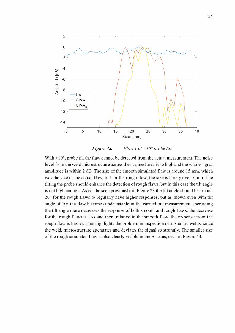
55
Figure 42. Flaw 1 at +10° probe tilt.
With +10°, probe tilt the flaw cannot be detected from the actual measurement. The noise
level from the weld microstructure across the scanned area is so high and the whole signal
amplitude is within 2 dB. The size of the smooth simulated flaw is around 15 mm, which
was the size of the actual flaw, but for the rough flaw, the size is barely over 5 mm. The
tilting the probe should enhance the detection of rough flaws, but in this case the tilt angle
is not high enough. As can be seen previously in Figure 28 the tilt angle should be around
20° for the rough flaws to regularly have higher responses, but as shown even with tilt
angle of 10° the flaw becomes undetectable in the carried out measurement. Increasing
the tilt angle more decreases the response of both smooth and rough flaws, the decrease
for the rough flaws is less and then, relative to the smooth flaw, the response from the
rough flaw is higher. This highlights the problem in inspection of austenitic welds, since
the weld, microstructure attenuates and deviates the signal so strongly. The smaller size
of the rough simulated flaw is also clearly visible in the B scans, seen in Figure 43.
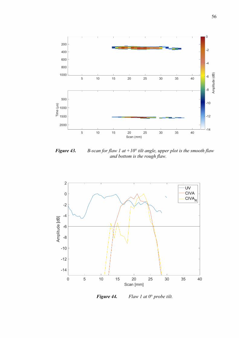
56
Figure 43. B-scan for flaw 1 at +10° tilt angle, upper plot is the smooth flaw
and bottom is the rough flaw.
Figure 44. Flaw 1 at 0° probe tilt.
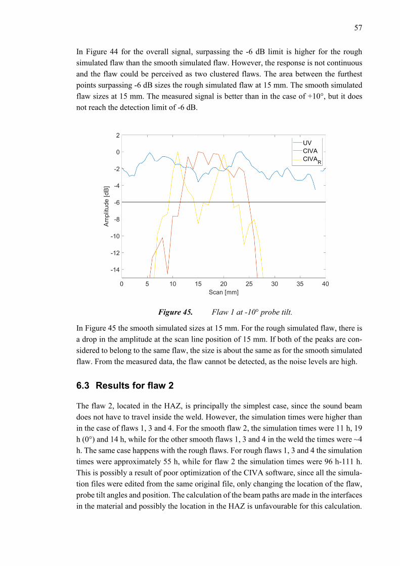
57
In Figure 44 for the overall signal, surpassing the -6 dB limit is higher for the rough
simulated flaw than the smooth simulated flaw. However, the response is not continuous
and the flaw could be perceived as two clustered flaws. The area between the furthest
points surpassing -6 dB sizes the rough simulated flaw at 15 mm. The smooth simulated
flaw sizes at 15 mm. The measured signal is better than in the case of +10°, but it does
not reach the detection limit of -6 dB.
Figure 45. Flaw 1 at -10° probe tilt.
In Figure 45 the smooth simulated sizes at 15 mm. For the rough simulated flaw, there is
a drop in the amplitude at the scan line position of 15 mm. If both of the peaks are con-
sidered to belong to the same flaw, the size is about the same as for the smooth simulated
flaw. From the measured data, the flaw cannot be detected, as the noise levels are high.
6.3 Results for flaw 2
The flaw 2, located in the HAZ, is principally the simplest case, since the sound beam
does not have to travel inside the weld. However, the simulation times were higher than
in the case of flaws 1, 3 and 4. For the smooth flaw 2, the simulation times were 11 h, 19
h (0°) and 14 h, while for the other smooth flaws 1, 3 and 4 in the weld the times were ~4
h. The same case happens with the rough flaws. For rough flaws 1, 3 and 4 the simulation
times were approximately 55 h, while for flaw 2 the simulation times were 96 h-111 h.
This is possibly a result of poor optimization of the CIVA software, since all the simula-
tion files were edited from the same original file, only changing the location of the flaw,
probe tilt angles and position. The calculation of the beam paths are made in the interfaces
in the material and possibly the location in the HAZ is unfavourable for this calculation.

58
The results of the measurements for flaw 2 are shown in figures Figure 46, Figure 47 and
Figure 48.
Figure 46. Flaw 2 at +10° probe tilt.
In Figure 46 the rough simulated flaw has an amplitude drop in the middle of the flaw.
The overall area from which the signal comes is also slightly smaller for the rough simu-
lated flaw than for the smooth simulated flaw. In the actual measurement, the detection
of the flaw is questionable. The biggest difference of the maximum and minimum ampli-
tudes is around -4 dB, so the overall noise level is high throughout the measured area.
The signal from the smooth simulated flaw has not changed much from the case of flaw
5 as expected due to the location in the HAZ.
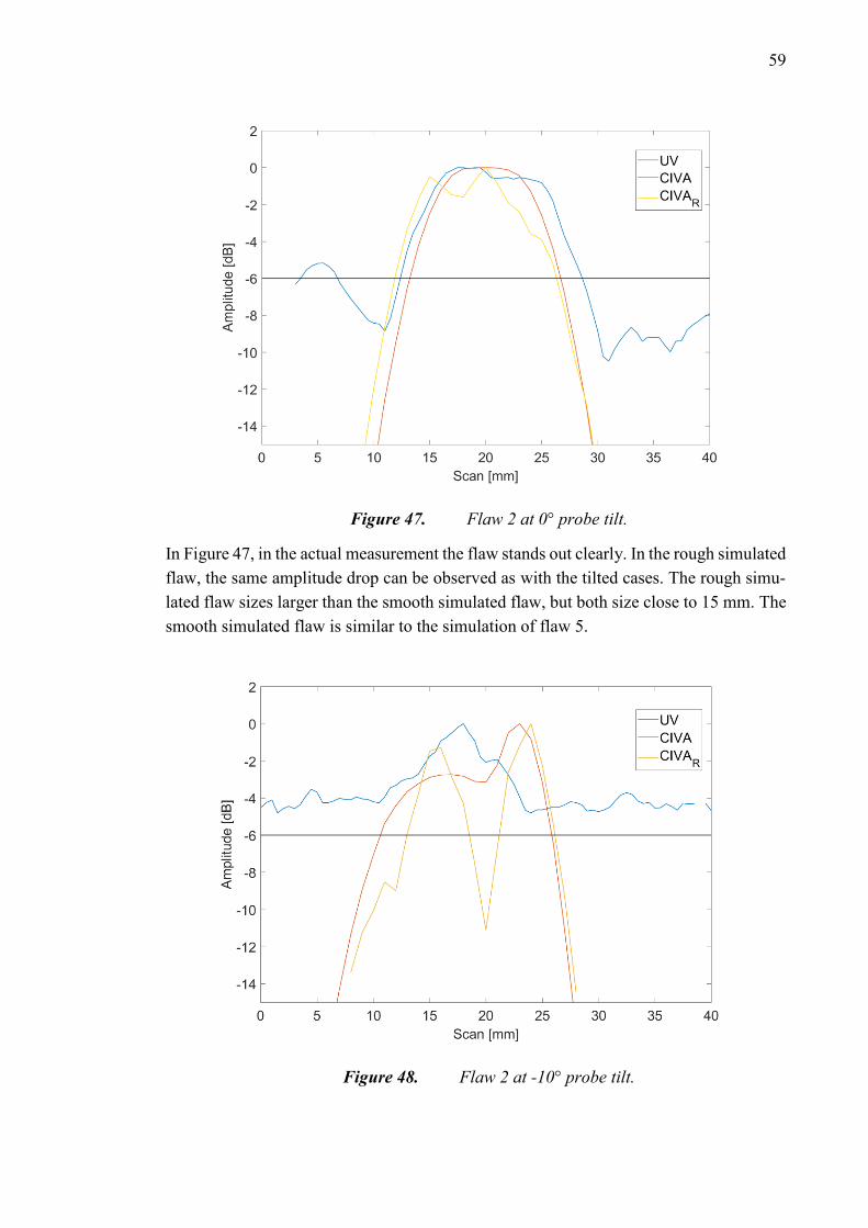
59
Figure 47. Flaw 2 at 0° probe tilt.
In Figure 47, in the actual measurement the flaw stands out clearly. In the rough simulated
flaw, the same amplitude drop can be observed as with the tilted cases. The rough simu-
lated flaw sizes larger than the smooth simulated flaw, but both size close to 15 mm. The
smooth simulated flaw is similar to the simulation of flaw 5.
Figure 48. Flaw 2 at -10° probe tilt.

60
For flaw 2 at -10° probe tilt the simulation was slightly altered, since the computation
would not complete. The scan line is only 20 mm, but it covers the area where the flaw
exists, hence it does not cover the whole area in Figure 48. The same amplitude drop in
the middle of the rough simulated flaw is observed as in the cases of 0° and +10°. The
amplitude peak to the left of the drop is lower than the one to the right. For the smooth
simulation, the area from which the signal comes from is slightly larger than in the case
of rough simulation. The actual measurement stands out from the data with an amplitude
difference of -4.5 dB to the noise. However, the signal seems to come from considerably
smaller area than the 15 mm that was the size of the flaw.
The amplitude drop observed in the simulation of the rough flaw in Figure 46, Figure 47
and Figure 48 could be verified from the CIVA simulation. At the point where the ampli-
tude drop occurs, the surface roughness of the flaw forms a concave shape to the sound
beam direction. As the sound beam reflects from the bottom of the specimen or directly
hits the concave surface and reflects primarily under the receiver. This is illustrated in
Figure 49.
Figure 49. Sound beam path of flaw 2 at -10° probe tilt.
The concave surface is not in the middle of the flaw, but the sound beam path can be seen
to divert below the probe as 10 beam lines are displayed. The maximum amplitude re-
sponse in this case is acquired near the right edge of the flaw.
6.4 Results for flaw 3
Flaw 3 was positioned 1 mm from the centre of the weld, towards the probe. Detection is
expected to be easier than in the case of flaw 1, since the distance for the sound beam
inside the weld is smaller. The results of measurements for flaw 3 are shown in Figure
50, Figure 52 and Figure 53

61
Figure 50. Flaw 3 at +10° probe tilt.
From the actual measurement in Figure 50, again flaw detection is not possible. The
smooth simulated flaw sizes at under 5 mm, which is considerably smaller than the actual
size of the flaw. In this case the tilting of the probe hinders the detection. The rough
simulated flaw instead sizes at over 15 mm and will be evaluated as larger than the orig-
inal flaw size. Two amplitude drops in the rough flaw are also detected. The amplitude
drops are due to the shape of the flaw and the threshold of the HAZ and weld in addition
with the weld structure. At 22 mm sound pressure is reflected below the probe in com-
parison with the 26 mm scan line with the maximum amplitude response, shown in Figure
51.
Figure 51. Rough simulated flaw 3 at +10° tilt beam paths, scan position of 22
mm on the left and 26 mm on the right with 11 rays displayed.

62
Figure 52. Flaw 3 at 0° probe tilt.
In Figure 52 the smooth simulated flaw is observed as larger than the rough simulated
flaw and it sizes at about 15 mm. The rough simulated flaw is slightly smaller and the
amplitude drops seen at the +10° case are not seen. From the carried out measurement the
flaw is not detectable with the -6 dB limit, but a clearer signal rises from the level of the
noise, making the detection possible.
Figure 53. Flaw 3 at -10° probe tilt.

63
For the -10° tilt angle, in Figure 53, the size of the rough simulated flaw is larger than the
smooth simulated flaw and exceeds 15 mm. However, an amplitude drop is seen between
the 10 and 15 mm scan line. The smooth simulated flaw has two amplitude drops and the
overall size is slightly larger than 15 mm. For the actual measurement, a drawn out peak
larger than the observed noise level can be detected. The peak does not stand out to reach
the -6 dB detection line, as the whole signal is within -4 dB, but the flaw can be detected.
Figure 54 shows the amplitude drop of the smooth simulated flaw. The flaw is located at
the edge of the HAZ and the weld, a small part of the bottom of the flaw is at the HAZ,
where the weld groove is located. The rest is positioned in the weld and the beams inter-
acting with the top of the flaw tend to reflect away due to the structure of the weld. The
amplitude drops occurs due to the weld structure and at the amplitude drops the sound
beams in the simulation can be seen to reflect upwards (16 mm scan), not reaching the
probe. Whereas in the case where the maximum amplitude peak is reached (15 mm scan)
the reflections are more optimal and a higher response is received. Highest pressure is
received from the sound beams that hit the bottom of the flaw located at the edge of the
weld and HAZ.
Figure 54. Smooth simulated flaw 3 at -10° tilt beam paths, scan position of 15
mm on the left and 16 mm on the right with 11 rays displayed.
Figure 55 shows the beam paths for the amplitude drop in the rough simulated flaw. The
amplitude drop at the 13 mm scan line is caused by the weld and HAZ structure, but also
strongly because the flaw again has a concave shape where the sound beam interacts with
the flaw, reflecting the sound under the probe. At 20 mm, where the maximum amplitude
is received more of the sound pressure is reflected back to the probe.

64
Figure 55. Rough simulated flaw 3 at -10° tilt beam paths, scan position of 13
mm on the left and 15 mm on the right with 11 rays displayed.
6.5 Results for flaw 4
Flaw 4 was principally the hardest case, the flaw is located furthest away in the weld, at
0.5 mm from the weld centre, away from the probe. The results are shown in Figure 56,
Figure 57 and Figure 59.
Figure 56. Flaw 4 at +10° probe tilt.
In Figure 56, the smooth simulated flaw has a stronger response, but it sizes under
15 mm. The rough simulated flaw sizes at even smaller, under 10 mm. From the
measured signal, the flaw cannot be detected.

65
Figure 57. Flaw 4 at 0° probe tilt.
In Figure 57, the smooth simulated flaw has bigger response compared to the actual flaw
size and the rough simulated flaw. The smooth simulated flaw sizes at over 20 mm as a
large scattered amplitude curve. The beam reflections and deviations inside the weld di-
vert the sound beams initially going past the flaw and response is received from a wider
area. This is shown in Figure 58. The rough simulated flaw sizes at under 10 mm. From
the actual measurement the flaw can be distinguished in the area between 15 and 30 mm
scan line, but the sizing is difficult due to the high noise levels.
Figure 58. Smooth simulated flaw 4 at 0° tilt beam paths, scan position of 29
mm with 11 rays displayed.

66
In Figure 58, the initial path where the rays are focused is shown with the faint orange
rectangle. The weld deviates the beams initially going past the weld and a strong response
is received, showing the difficulty in locating the exact position from where the echo is
received inside an austenitic stainless steel weld.
Figure 59. Flaw 4 at -10° probe tilt.
In Figure 59, the rough simulated flaw sizes at over 15 mm, but again an amplitude drop
is observed, shown in Figure 60. The smooth simulated flaw sizes under 15 mm. From
the measurement, the flaw cannot be detected.

67
Figure 60. Rough simulated flaw 4 at -10° tilt beam paths, scan position of 17
mm on the top and 20 mm on the bottom with 11 rays displayed.
In Figure 60, the concave surface of the flaw again diverts the beams under the probe at
the 17 mm scan line, whereas in the 20 mm position, where the maximum response was
acquired more rays return to the probe. In this case, the weld structure also diverts beams
that would travel to the concave surface to other parts of the flaw, so the amplitude drop
is not as severe as in the case of flaw 2 -10° tilt angle, where the flaw is located in the
HAZ. Also even in the maximum response position more complex beam paths, going
even further to the weld after reflecting with the flaw are observed.
6.6 Improvements
The mount of the probe to the scanning system was not completely rigid. A more perma-
nent solution to the probe mounting would eliminate the movement of the probe. The
scanning was done as a raster type scan, so every other scan line is done from different
side, to X and -X, directions. This means the probe might be at slightly different positions
for every other scan line. Comb scan could be used to always have the same scanning
direction, but this would increase the scanning time.

68
The rotation of the probe to +10° and -10° tilt angles was done by hand. A third motor to
allow the precise rotation around the Z-axis would make the control of the tilt angle more
accurate.
In the simulations, the rough flaws were done individually for each different flaw. The
overall surface roughness was the same, but there is variation within the flaws. Using the
exact same flaw could improve the comparability of the results of different flaws.
Using all of the available angles for the used probe 40°-70° would improve the results of
the actual measurements, but only one angle was used to limit the simulation times.
The simulation accuracy could be improved, but all improvements come with the cost of
simulation time. As the weld structure, a premade stiffness matrix from CIVA was used.
This could be also constructed from an example piece done with the same properties, but
would induce costs and time. The concave surface in the flaw caused amplitude drops in
the flaw response signal. Adding structural noise and attenuation levels would improve
the comparability with the carried out measurements. As the used scanning step was 0.5
mm the sizing accuracy could be improved with smaller scanning steps. In the simulation,
adding more probe scanning angles the results would improve, and the frequent amplitude
drops due to the flaw structure might be avoided. As the scans were done with just one
scan line in the direction of the probe length, adding more scan lines would yield results
that are more precise. Another possibility would be the utilization of total focusing
method, where each element takes turn transmitting, while all elements are receiving [62].
The wanted improvements in accuracy need to be evaluated with the increased simulation
time to find an optimal solution.
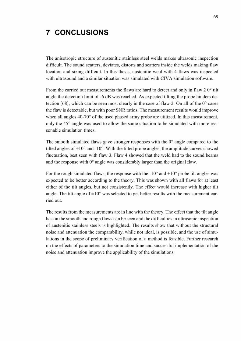
69
7 CONCLUSIONS
The anisotropic structure of austenitic stainless steel welds makes ultrasonic inspection
difficult. The sound scatters, deviates, distorts and scatters inside the welds making flaw
location and sizing difficult. In this thesis, austenitic weld with 4 flaws was inspected
with ultrasound and a similar situation was simulated with CIVA simulation software.
From the carried out measurements the flaws are hard to detect and only in flaw 2 0° tilt
angle the detection limit of -6 dB was reached. As expected tilting the probe hinders de-
tection [68], which can be seen most clearly in the case of flaw 2. On all of the 0° cases
the flaw is detectable, but with poor SNR ratios. The measurement results would improve
when all angles 40-70° of the used phased array probe are utilized. In this measurement,
only the 45° angle was used to allow the same situation to be simulated with more rea-
sonable simulation times.
The smooth simulated flaws gave stronger responses with the 0° angle compared to the
tilted angles of +10° and -10°. With the tilted probe angles, the amplitude curves showed
fluctuation, best seen with flaw 3. Flaw 4 showed that the weld had to the sound beams
and the response with 0° angle was considerably larger than the original flaw.
For the rough simulated flaws, the response with the -10° and +10° probe tilt angles was
expected to be better according to the theory. This was shown with all flaws for at least
either of the tilt angles, but not consistently. The effect would increase with higher tilt
angle. The tilt angle of ±10° was selected to get better results with the measurement car-
ried out.
The results from the measurements are in line with the theory. The effect that the tilt angle
has on the smooth and rough flaws can be seen and the difficulties in ultrasonic inspection
of austenitic stainless steels is highlighted. The results show that without the structural
noise and attenuation the comparability, while not ideal, is possible, and the use of simu-
lations in the scope of preliminary verification of a method is feasible. Further research
on the effects of parameters to the simulation time and successful implementation of the
noise and attenuation improve the applicability of the simulations.

70
REFERENCES
1. Koskinen, T., & Examiner, M. V. (2015). Artificial Flaw Detection with
Ultrasound in Austenitic Stainless Steel.
2. Lippold, John C.; Kotecki, D. J. (2005). 1. Introduction. In Welding Metallurgy
and Weldability of Stainless Steels (pp. 2–6). John Wiley & Sons.
3. Ashby, Michael F.; Jones, D. R. H. (2013). Engineering Materials 2 - An
Introduction to Microstructures and Processing (4th ed., pp. 221–230).
4. Mathers, G. (2014). Welding of austenitic stainless steel. TWI Ltd. Retrieved
January 15, 2018, from https://www.twi-global.com/technical-knowledge/job-
knowledge/welding-of-austenitic-stainless-steel-103/
5. IMOA (International Molybdeum Association). (2010). 3. Metallurgy. In Practical
Guidelines for the Fabrication of High Performance Austenitic Stainless Steels
(pp. 3–12).
6. Phillips, D. H. (2015). 11 Welding Metallurgy of Stainless Steels. In Welding
Engineering : An Introduction (pp. 203–217). John Wiley & Sons, Incorporated.
7. Ehrnstén, U. (2012). Corrosion and stress corrosion cracking of austenitic stainless
steels. Comprehensive Nuclear Materials, 5, 93–104. doi:10.1016/B978-0-08-
056033-5.00080-X
8. Mathers, G. (n.d.). Welding of austenitic stainless steel. Part 2, Job Knowledge
104. The Welding Institute, TWI. Retrieved June 12, 2018, from https://www.twi-
global.com/technical-knowledge/job-knowledge/welding-of-austenitic-stainless-
steel-part-2-104/
9. William D. Callister, J. (2007). 9. Phase Diagrams. In Materials Science and
Engineering an Introduction (p. 255).
10. McGuire, M. F. (2008). 6. Austenitic Stainless Steels. In Stainless Steels for Design
Engineers (pp. 69–90). ASM International.
11. Bhadeshia, H., & Honeycombe, R. (2006). 5. Formation of Martensite. In Steels -
Microstructure and Properties (3rd Edition) (pp. 95–128). Elsevier.
12. Primary Metallic Crystalline Structures (BCC, FCC, HCP). (n.d.). NDT Resource
Center. Retrieved from https://www.nde-
ed.org/EducationResources/CommunityCollege/Materials/Structure/metallic_stru
ctures.htm
13. Bhadeshia, H., & Honeycombe, R. (2006). 1. Iron and its Interstitial Solid
Solutions. In Steels - Microstructure and Properties (3rd Edition) (pp. 1–16).
Elsevier.

71
14. William D. Callister, J. (2007). 3. The Structure of Crystalline Solids. In Materials
Science and Engineering an Introduction (pp. 40–44). John Wiley & Sons,
Incorporated.
15. Fukai, Y. (2005). 2 Phase Diagrams and Statistical Thermodynamics of Binary M–
H Systems. In The Metal-Hydrogen System (Vol. 21, p. 31).
16. Bhadeshia, H., & Honeycombe, R. (2006). 12. Stainless Steel. In Steels -
Microstructure and Properties (pp. 259–286). Elsevier.
17. Lippold, John C.; Kotecki, D. J. (2005). 6. Austenitic Stainless Steels. In Welding
Metallurgy and Weldability of Stainless Steels (pp. 141–229). John Wiley & Sons.
18. Lister, D. H. (2012). 2.6 Stainless steels. In Nuclear Corrosion Science and
Engineering (pp. 43–47). doi:10.1533/9780857095343.1.57
19. AK Steel. (2007). 304/304L Stainless steel. AK Steel Data sheet.
doi:10.1038/041416a0
20. AK Steel. (2016). 316/316l Stainless steel. AK Steel Data sheet. Retrieved
February 9, 2018, from
http://www.aksteel.com/pdf/markets_products/stainless/austenitic/316-
316L_Stainless_Steel_PDB_201706.pdf
21. AK Steel. (2015). 321 Stainless Steel. AK Steel Data sheet. Retrieved February 9,
2018, from
http://www.aksteel.com/pdf/markets_products/stainless/austenitic/321_Stainless_
Steel_DS_201512.pdf
22. Lampman, S. R. (1997). Weld Solidification. Weld Integrity and Performance, 6,
3–22.
23. Inoue, H., Koseki, T., Okita, S., & Fuji, M. (1997). Solidification and
transformation behaviour of austenitic stainless steel weld metals solidified as
primary austenite: Study of solidification and subsequent transformation of Cr-Ni
stainless steel weld metals (2nd Report). Welding International, 11(12), 937–949.
doi:10.1080/09507119709447349
24. Cui, Y., & Lundin, C. D. (2007). Austenite-preferential corrosion attack in 316
austenitic stainless steel weld metals. Materials and Design, 28(1), 324–328.
doi:10.1016/j.matdes.2005.05.022
25. KATAYAMA, S., FUJIMOTO, T., & MATSUNAWA, A. (1985). Correlation
among solidification process, microstructure, microsegregation and solidification
cracking susceptibility in stainless steel weld metals.
26. Thompson, A. W. (1984). A Fundamental Study of the Beneficial Effects of Delta
Ferrite in Reducing Weld Cracking. Welding Reseach, 71–83.
27. Inoue, H., Koseki, T., Okita, S., & Fuji, M. (1997). Solidification and
transformation behaviour of austenitic stainless steel weld metals solidified as
primary ferrite: Study of solidification and subsequent transformation of Cr-Ni

72
stainless steel weld metals (2nd Report). Welding International, 11(12), 937–949.
doi:10.1080/09507119709447349
28. Sensitisation of Austenitic Stainless Steels. (n.d.). Austral Wright Metals.
Retrieved February 6, 2018, from http://www.australwright.com.au/sensitisation-
of-austenitic-stainless-steels/
29. Easwaran, R ;Raju, N ;Ravichandran, G; Sudharsanam, V. (2013). Distortion and
its Control in Welding of Stainless Steel Structures - Case Studies. Century of
Stainless Steels : Selected, Peer Reviewed Papers from the Stainless Steel
Centenary Symposium (SSCS 2013), 794(Advanced Materials Research Vol.794
(2013)), 358–365. Retrieved from
http://ku4jd9mg2y.search.serialssolutions.com/?ctx_ver=Z39.88-
2004&ctx_enc=info%3Aofi%2Fenc%3AUTF-
8&rfr_id=info%3Asid%2Fsummon.serialssolutions.com&rft_val_fmt=info%3Ao
fi%2Ffmt%3Akev%3Amtx%3Abook&rft.genre=proceeding&rft.title=Advanced
+Materials+Research&
30. Kain, V. (2011). Stress corrosion cracking (SCC) in stainless steels. In Stress
corrosion cracking: Theory and practice. doi:10.1533/9780857093769.3.199
31. Andresen, P. L., & Was, G. S. (2012). Irradiation assisted stress corrosion
cracking. Comprehensive Nuclear Materials (Vol. 5). Elsevier Inc.
doi:10.1016/B978-0-08-056033-5.00084-7
32. Andersen, P. (2012). 6. Irradiation assisted corrosion and stress corrosion cracking
(IAC/IASCC) in nuclear reactor systems and components. In Nuclear Corrosion
Science and Engineering (pp. 131–176).
33. Miura, T., Fujii, K., Fukuya, K., & Ito, Y. (2009). Characterization of deformation
structure in ion-irradiated stainless steels. Journal of Nuclear Materials, 386–
388(C), 210–213. doi:10.1016/j.jnucmat.2008.12.093
34. Chung, H. M., Ruther, W. E., Sanecki, J. E., Hins, A., Zaluzec, N. J., & Kassner,
T. F. (1996). Irradiation-assisted stress corrosion cracking of austenitic stainless
steels: recent progress and new approaches. Journal of Nuclear Materials, 239,
61–79. doi:10.1016/S0022-3115(96)00677-0
35. Shankar, V., Gill, T. P. S., Mannan, S. L., & Sundaresan, S. (2003). Solidification
cracking in austenitic stainless steel welds. Sadhana, 28(3–4), 359–382.
doi:10.1007/BF02706438
36. Lee, D. J., Byun, J. C., Sung, J. H., & Lee, H. W. (2009). The dependence of crack
properties on the Cr/Ni equivalent ratio in AISI 304L austenitic stainless steel weld
metals. Materials Science and Engineering A, 513–514(C), 154–159.
doi:10.1016/j.msea.2009.01.049
37. Bruscato, R. M. (1992). Liquid Metal Embrittlement of Austenitic Stainless Steel
When Welded to Galvanized Steel. Welding Journal, 455–460.
38. Li, S., et al. (2011). The Effect of Helium on Welding Irradiated Materials.
Welding Journal, 90(1), 19S–26S. Retrieved from

73
https://app.aws.org/wj/supplement/wj201101_s19.pdf
39. Krautkrämer, J., & Krautkrämer, H. (1983). Ultrasonic Testing of Materials.
40. Palanichamy, P., Joseph, A., Jayakumar, T., & Raj, B. (1995). Ultrasonic velocity
measurements for estimation of grain size in austenitic stainless steel. NDT & E
International, 28(3), 179–185. doi:10.1016/0963-8695(95)00011-L
41. Sound propagation in Elastic Materials. (n.d.). NDT Resource Center. Retrieved
May 9, 2018, from https://www.nde-
ed.org/EducationResources/CommunityCollege/Ultrasonics/Physics/elasticsolids.
php
42. Williams, D. (2012). The physics of ultrasound. Imaging and Technology in
Urology: Principles and Clinical Applications, 9781447124(6), 23–26.
doi:10.1007/978-1-4471-2422-1_6
43. Wave Propagation. (n.d.). NDT Resource Center. Retrieved March 15, 2018, from
https://www.nde-
ed.org/EducationResources/CommunityCollege/Ultrasonics/Physics/wavepropag
ation.htm
44. Cheeke, J. D. N. (2002). Fundamentals and Applications of Ultrasonic Waves.
Retrieved from https://books.google.com/books?id=Lnzb4PeTbeYC&pgis=1
45. Kenny, P. G. (2015). Ultrasonic Inspection, Attenuation of Ultrasonic. In ASM
Handbook, Volume 17, Nondestructive Evaluation and Quality Control (Vol. 17,
pp. 1–16).
46. Louis Cartz. (1995). Chapter III Ultrasonic Testing. In Nondestructive Testing:
Radiography, Ultrasonics, Liquid Penetrant, Magnetic Particle, Eddy Current (pp.
81–125).
47. Campbell, F. C. (2013). 11. Ultrasonic Inspection. In Inspection of Metals -
Understanding the Basics (pp. 267–292). ASM International. Retrieved from
http://ku4jd9mg2y.search.serialssolutions.com/?ctx_ver=Z39.88-
2004&ctx_enc=info%3Aofi%2Fenc%3AUTF-
8&rfr_id=info%3Asid%2Fsummon.serialssolutions.com&rft_val_fmt=info%3Ao
fi%2Ffmt%3Akev%3Amtx%3Abook&rft.genre=book&rft.title=Inspection+of+
Metals&rft.au=Campbe
48. Reflection and Transmission Coefficients (Pressure). (n.d.). NDT Resource Center.
Retrieved March 16, 2018, from https://www.nde-
ed.org/EducationResources/CommunityCollege/Ultrasonics/Physics/reflectiontra
nsmission.htm
49. IOlympus, N. (2006). Ultrasonic transducers technical notes. Technical brochure:
Olympus NDT, Waltham, MA, 39–49. Retrieved from
http://scholar.google.com/scholar?hl=en&btnG=Search&q=intitle:Ultrasonic+Tra
nsducers+Technical+Notes#0
50. GORNAJA, S. P., & ALJOSHIN, N. P. (1997). Attenuation of Ultrasonic Waves
74
in Austenitic Steel Welds. Nondestructive Testing and Evaluation, 13(3), 149–168.
doi:10.1080/10589759708953026
51. Léger, A., Deschamps, M., GDR 2501 (Research network), & SpringerLink
(Online service). (2009). Ultrasonic Wave Propagation in Non Homogeneous
Media. Springer proceedings in physics, (Vol. 128). doi:10.1007/978-3-540-
89105-5
52. Kenny, P. G. (2015). Ultrasonic Inspection, Transducer Elements. In ASM
Handbook, Volume 17, Nondestructive Evaluation and Quality Control (Vol. 17,
pp. 18–21).
53. Kenny, P. g. (2015). Ultrasonic Inspection, Search Units. In ASM Handbook,
Volume 17, Nondestructive Evaluation and Quality Control (Vol. 17, pp. 1–11).
54. Signal-to-Noise Ratio. (n.d.). NDT Resource Center. Retrieved June 19, 2018,
from https://www.nde-
ed.org/EducationResources/CommunityCollege/Ultrasonics/Physics/signaltonois
e.htm
55. Sfs, S. S. (2012). SFS-EN ISO 16810 Non-destructive testing. Ultrasonic testing.
General principles, 23.
56. FINNISH STANDARDS ASSOCIATION SFS. (2011). SFS-EN ISO 11666 Non-
destructive testing of welds. Ultrasonic testing. Acceptance levels.
57. Howard, P. J., Copley, D. C., & Gilmore, R. S. (1995). A Signal-to-Noise Ratio
Comparison of Ultrasonic Transducers for C-Scan Imaging. Review of Progress in
Quantitative Nondestructive Evaluation, 14(1), 2113–2120. doi:10.1007/978-1-
4615-1987-4_270
58. Kenny, P. G. (2015). Ultrasonic Inspection, Pulse-Echo Methods. In ASM
Handbook, Volume 17, Nondestructive Evaluation and Quality Control (Vol. 17,
pp. 1–17).
59. Data Presentation. (n.d.). NDT Resource Center. Retrieved April 26, 2016, from
https://www.nde-
ed.org/EducationResources/CommunityCollege/Ultrasonics/EquipmentTrans/Dat
aPres.htm
60. Mathers, G. (n.d.). Ultrasonic examination Part 1-3. The Welding Institute, TWI.
Retrieved April 27, 2018, from https://www.twi-global.com/technical-
knowledge/job-knowledge/ultrasonic-examination-part-1-127/
61. R. Nave. (n.d.). Huygens’ Principle. Hyperphysics. Retrieved May 3, 2018, from
http://hyperphysics.phy-astr.gsu.edu/hbase/phyopt/huygen.html
62. Lester W. Schmerr Jr. (2012). Fundamentals of Ultrasonic Phased Arrays.
doi:10.1007/978-94-007-4282-6
63. Bulavinov, A., Kröning, M., & Walte, F. (2007). Ultrasonic Inspection of
Austenitic and Dissimilar Welds. Proceedings of the IV Conferencia

75
Panamericana de END, 13.
64. Olympus. (n.d.). Focusing With Phased Array Probes. Phased Array Tutorial.
Retrieved July 23, 2018, from https://www.olympus-ims.com/en/ndt-
tutorials/transducers/focusing/
65. Olympus. (n.d.). Phased Array Transducer Characteristics. Phased Array Tutorial.
Retrieved May 3, 2018, from https://www.olympus-ims.com/en/ndt-
tutorials/transducers/pa-definitions/
66. Olympus. (n.d.). Beam Shaping. Phased Array Tutorial. Retrieved May 3, 2018,
from https://www.olympus-ims.com/en/ndt-tutorials/transducers/pa-
beam/shaping/
67. Olympus. (n.d.). Beam Steering. Phased Array Tutorial. Retrieved May 3, 2018,
from https://www.olympus-ims.com/en/ndt-tutorials/transducers/pa-
beam/steering/
68. Kemppainen, M., & Virkkunen, I. (2011). Crack characteristics and their
importance to NDE. Journal of Nondestructive Evaluation, 30(3), 143–157.
doi:10.1007/s10921-011-0102-z
69. Pettit, J. R., Walker, A. E., & Lowe, M. J. S. (2015). Improved detection of rough
defects for ultrasonic nondestructive evaluation inspections based on finite element
modeling of elastic wave scattering. IEEE Transactions on Ultrasonics,
Ferroelectrics, and Frequency Control, 62(10), 1797–1808.
doi:10.1109/TUFFC.2015.007140
70. Zhang, J., Drinkwater, B. W., & Wilcox, P. D. (2012). Effect of Roughness on
Imaging Defects Using Ultrasonic Arrays, 59(5), 939–948.
71. Wirdelius, H., & Osterberg, E. (2000). SKI Report 00 : 42 Study of Defect
Characteristics Essential for NOT Testing Methods ET, UT and RT, (October), 1–
58.
72. Iida, K., Takumi, K., & Naruse, A. (1988). Influence of stress condition on flaw
detectability and sizing accuracy by ultrasonic inspection. Retrieved from
https://inis.iaea.org/search/search.aspx?orig_q=RN:21053909
73. Report, P. I. (n.d.). Integration of N DE Reliability and Fracture Mechanics, 1.
74. Crutzen, S., Lemaitre, P., & Iacono, I. (1996). Realistic Defects Suitable for ISI
Capability Evaluation and Qualification. Proceedings of the 14th International
Conference on NDE in the Nuclear and Pressure Vessel Industries, 153–163.
75. NDE. (n.d.). CIVA 2017 user manual.
76. Extende. (n.d.). CIVA in a few words. Retrieved August 3, 2018, from
http://www.extende.com/civa-in-a-few-words
77. Shivanna, D. M., Kiran, M. B., & Kavitha, S. D. (2014). Evaluation of 3D Surface
Roughness Parameters of EDM Components Using Vision System. Procedia

76
Materials Science, 5, 2132–2141. doi:10.1016/j.mspro.2014.07.416

77
APPENDIX A: RESULTS WITH TWO AMPLITUDE AXES
The results for the flaws are shown with two different amplitude axes in Figure 61, Figure
62, Figure 63, Figure 64 and Figure 65. The axis on the left hand size is for the carried
out measurement and the axis on the right is for the rough and smooth simulated flaws.
This is done to give a view of the shape of the full amplitude curve.

78
Figure 61. Results for flaw 5 with different amplitude axes, top for +10°, mid-
dle for 0° and bottom for -10° probe tilt angle.

79
Figure 62. Results for flaw 1 with different amplitude axes, top for +10°, mid-
dle for 0° and bottom for -10° probe tilt angle.

80
Figure 63. Results for flaw 2 with different amplitude axes, top for +10°, mid-
dle for 0° and bottom for -10° probe tilt angle.

81
Figure 64. Results for flaw 3 with different amplitude axes, top for +10°, mid-
dle for 0° and bottom for -10° probe tilt angle.
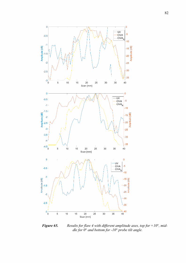
82
Figure 65. Results for flaw 4 with different amplitude axes, top for +10°, mid-
dle for 0° and bottom for -10° probe tilt angle.
83
APPENDIX B: B-SCANS FOR FLAWS 1-4
B-scans for flaws 1-4 are shown in Figure 66, Figure 67, Figure 68 and Figure 69. From
the b-scans the size can be seen more clearly. The sizing at -6 dB corresponds to yellow
color as seen from the colorbar. The upper plot of each figure refers to the smooth simu-
lated flaw and the lower one to the rough simulated flaw. The B-scan for flaw 2 at -10° is
not shown due to problems in the simulation of the rough flaw.

84
Figure 66. B-scans for flaw 1, up +10°, middle 0° and bottom -10° tilt angle.

85
Figure 67. B-scans for flaw 2, up +10°and bottom 0° tilt angle.

86
Figure 68. B-scans for flaw 3, up +10°, middle 0° and bottom -10° tilt angle.
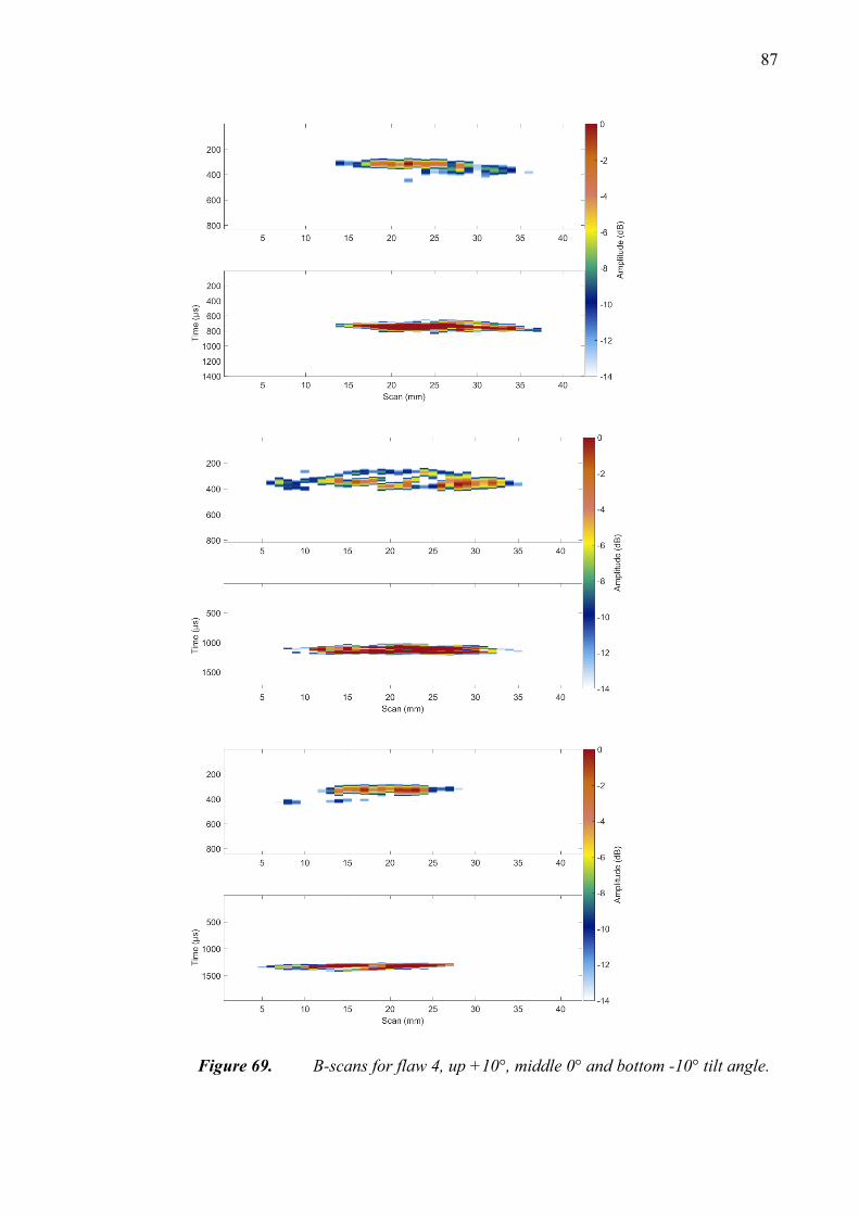
87
Figure 69. B-scans for flaw 4, up +10°, middle 0° and bottom -10° tilt angle.