UNIT-1MANAGERIAL ECONOMICS

Managerial Economic Managerial Economics is economicapplied in decision - making. It is that branch of economicswhich serves as a link between abstract theory and managerialpractice. It is based on economic analysis for identifying problems,organising information & evaluation alternatives.

Economics as a science is concerned with the problem ofallocation of scarce resources among competing ends. Theseproblems of allocation are regularly confronted by individuals,households, firms as well as economies. Economics is able toprovide a number of sophisticated concepts and analytical toolsand understand and analyse such problems managerialeconomics when seen in this lights, may be taken as economicsapplied to problems of choice of alternatives of economic natureand allocation of scarce resource by the firms. In other wordsmanagerial economies involves analysis of allocation of theseresources available to a firm or a unit of management amongthe activities of that unit.Definitions:1. Managerial economics is the use of economic modes ofthought to analyse business situation” McNair and Meriam.2. Managerial economics is the integratic of economic theorywith business practice for the purpose of facilitating decisionmaking and forward planning by management - Spencer &Siegelman.NATURE OF MANAGERIAL ECONOMICS

Managerial economics is concerned with the business firmand the economic problems that every business managementneed to solve. Spencer and Siegelman point to the fact that“Managerial Economics is the integration of economic theoryand business practice for the purpose of facilitating decision -making and forward planning by management. Before we lookinto this integration aspect let us first study the nature ofeconomic theory considered relevant for managerial decisionmaking.

Macro - economic Conditions: We know that the decisionsof the firm are made almost always with in the broad frameworkof economic environment within which the firm operates, knownas macro-economic conditions with regard to these conditions,we may stress three points.

Positive approach concerns with what is was or will bewhile normative approach concerns with what ought to be. Thestatement a government deficit will reduce unemployment andcause an increase in prices is a hypothesis in positive economics,while the statement in setting policy unemployment ought tomatter more than inflation is a normative hypothesis.

Integration of Economic Theory & Business Practice: Acritical look (a) with the help of economic theory one canunderstand the actual business behaviour. This does not meanthat in economics there is always a theoretical construct presentfor every business behaviour. In fact, economic theory is basedon certain assumption, and sometimes very simplifiedassumptions.b) managerial economies attempts to estimate and predict theeconomic qualities and relationships. The estimation of elasticityof demand, production relation, are all necessary for the purposesof forecasting by the firm. Similary predicting about the demand,cost, pricing etc is needed for decision making.SCOPE OF MANAGERIAL ECONOMICS:

Managerial economics has a choice connection willeconomic theory (micro-economics as well as micro-economics)operations, research, statistics, mathematics, and the theory ofdecision - making - managerial economics also draws togetherand relates ideas from various functional areas of managementlike production marketing, finance and accounting projectmanagement etc.

In so far as managerial economics is concerned, thefollowing aspects constitute its subject-matter.i) Objectives of a business firmii) Demand Analysis and Demand forecasting.iii) Production and cost.iv) Competition

v) Pricing and outputvi) Profitvii) Investment and caital budgeting andviii) Product policy, sales promotion and market strategy.MANAGERIAL ECONOMICS AND OPERATIONS RESEARCH

In general the relation between managerial economicsare concerned with taking effective decisions. Given the firm’sobjectives, both are concerned with what is th ebest way ofachieving them. the difference, however, is: managerialeconomics is a fundamental academic subject which seeks tounderstand and to analyse the problems of business decision -taking, while operations research is an activity carried out byfunctional specialists for solving decision problems.MANAGERIAL ECONOMICS AND TRADITIONAL ECONOMICS:

In general the relation between managerial economicsand economic theory is very much like the relation of engineeringto physics & of machine to biology. It is in fact the relatin of anapplied field to its more fundamental & conceptual counter part.Economics provides certain basic concepts and analytical toolswhich are applied suitably to a business situation.

Further, while economists mainly concentrate on thestudy of types of makes, managerial economists are concernedmore with problems like the impacts of market or technologicalchanges on competitive position of the firm and the likely reactionsof their own actions in the market. But managerial economistcan get answers of the questions regarding the working of marketmechanism only when they analyse the problems from a broaderperspective of an economist.

Thus, the two main contribution of economics to mangerialeconomies are:* To help in understanding the market & the general environmentwith a which the firm operates.* To provide a philosophy for understandings & analyzing resource- allocation problems.

MANAGEMENT ECONOMICS AND MATHEMATICSMathematics provides us with a set of tools which help in

the derivation and exposition of economic analysis. Mathematicsis closely related to managerial economics. This is mainlybecause the managerial economics, besides conceptual, is alsomaterial. It derives its metrical property from the set fact thatan individual function of managerial economics is to estimateand predict the relevant economic factors for decision makingand forward planning.

MANAGERIAL ECONOMICS AND STATISTICSStatistics is widely used by managerial economists.

Managerial economies aims at quantifying the past economicsactivity as well as to predict its future course. This is neededfor a correct judgement and decision-making.MANAGERIAL ECONOMICS AND THE THEORY OF DECISION

MAKINGThe theory of decision making is relatively a new subject

that has significance for managerial economics. Much ofeconomic theory is based on the assumption of a single goalmaximization of profit for the firm or maximization of utility of aconsumer.

RESPONSIBILITIES OF MANAGERIAL ECONOMISTThe most important of hte obligations of a managerial

economist is that his objectives must coincide with that of thebusiness. Since in most of the cases the firms try to maximizeprofits on their invested capital, the managerial economist mustalso help in achieving this goal. so long as he maintains thatconviction and helps in enhancing the ability of the firm tomaximize profits he will be a successful managerial economics.

The other most important responsibility of a managerialeconomist is to try to make as accurate forecasts as possible.We know that every decision a management takes normally hasimplications going beyond the present while, on the other hand,future is rather uncertain. It is, therefore, necessary andobligatory ofr a managerial economist to make future forecastsin such a manner that the risks involved in the uncertainties offuture are minimized for the firm.

If a managerial economist can keep on providing successfulforecasts at the required time, he is bound to be a successfulexecutive. Here a couple of important points need be mentioned.First if the managerial economist finds that due to some suddenand unaccounted factors, the presented forecast has undergonea change. It is duty to work out the new forecast and present itat the earliest possible time.

ELASTICITY OF DEMANDWe have seen that changes in product, income of the

households, prices of related goods, tastes and expectations,advertising, expenses etc. effect quantity demanded of a good.This indicates only directional impact of the changes in thefactors influencing demand. Since change in any demanddeterminant does not affect the demand of every good to thesame extent (e.g. a change in income level of the consumers donot affect their demand for clothing equally)

This ability to predict revenue is crucial as without anadequate level of sales relative to costs the firm cannot besuccessful. Fortunately, the economist has a tool to measurethe effect of changes in any one of hte determinants in th demandfunction, which helps us in providing a quantitative value for theresponsiveness of the quantity demanded change in each of thedeterminants in the demand function. Elasticity of demand (ED)is defined a the percentage change in quantity demanded causedby one percent change in demand determinant underconsideration, while other determinants are held constant. Thegeneral equation for the measurement of elasticity of demandis.E = Percentage change in quantity demanded of goods Percentage change in ddeterminant Z

The larger the (absolute) valve of this elasticity, the moreresponsive is quantity demanded to changes in the determinantunder consideration. If we look at the demand function, we cannotice that certain determinants of demand are completelybeyond the control of the firm. The firm cannot possibly makeany significant difference to average annual income of theconsumers, the number of consumers of the prices of the relatedgoods.

TYPES OF ELASTICITY OF DEMAND AND THEIRMANAGERIAL USES

Elasticity of demand is the degree of change in demandcaused by change in price. This concept was introduced by AlfredMarshall. But the applied this concept only to the price demand.

According to Alfred Marshall: The elasticity of demand isgreat are small according as the amount demanded increasemuch are little for given fall in price and diminishes much arelittle for a given rise in price.

Elasticity demanded proportionate change in demand.Proportionate change in price

QPx

PQ

ΔΔ

The concept of elasticity of demand was later developedby modern economists who applied this concept to the incomeand gross demands.

TYPES OF ELASTICITY OF DEMANDThe price elasticity of demand is of 5 types.

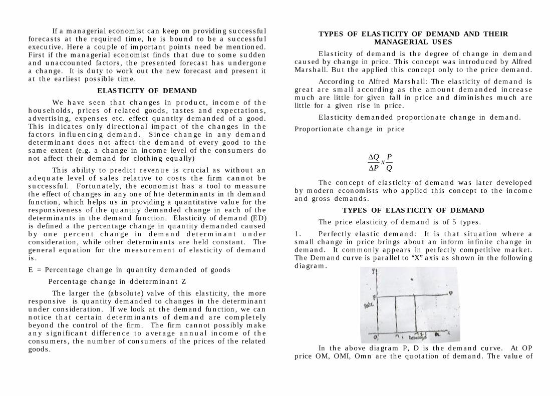
1. Perfectly elastic demand: It is that situation where asmall change in price brings about an inform infinite change indemand. It commonly appears in perfectly competitive market.The Demand curve is parallel to “X” axis as shown in the followingdiagram.

In the above diagram P, D is the demand curve. At OPprice OM, OMI, Omn are the quotation of demand. The value of

perfectly elastic demand is α

%0%50

==ΔΔ

= EdPDEd

Ed=α

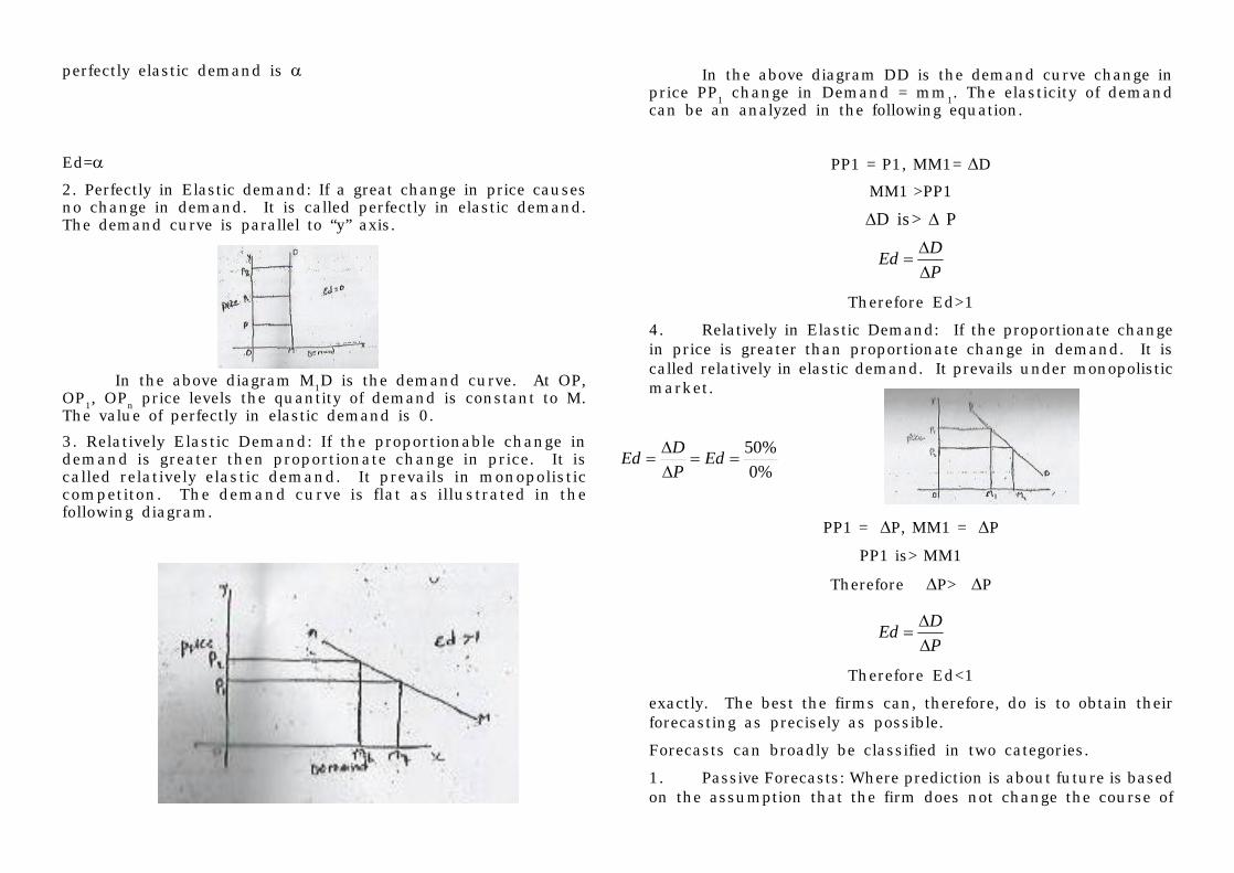
2. Perfectly in Elastic demand: If a great change in price causesno change in demand. It is called perfectly in elastic demand.The demand curve is parallel to “y” axis.

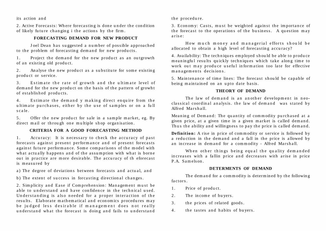
In the above diagram M1D is the demand curve. At OP,OP1, OPn price levels the quantity of demand is constant to M.The value of perfectly in elastic demand is 0.3. Relatively Elastic Demand: If the proportionable change indemand is greater then proportionate change in price. It iscalled relatively elastic demand. It prevails in monopolisticcompetiton. The demand curve is flat as illustrated in thefollowing diagram.

In the above diagram DD is the demand curve change inprice PP1 change in Demand = mm1. The elasticity of demandcan be an analyzed in the following equation.

PP1 = P1, MM1= ΔD

MM1 >PP1

ΔD is> Δ P

PDEd

ΔΔ

=

Therefore Ed>1

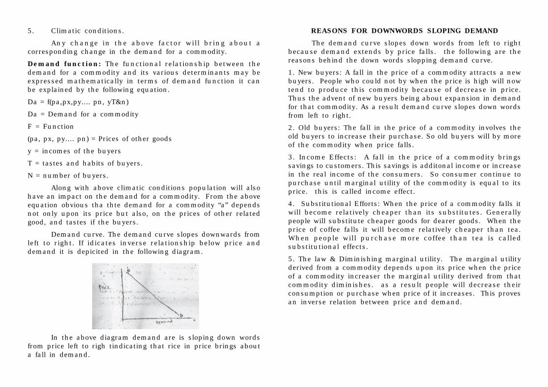
4. Relatively in Elastic Demand: If the proportionate changein price is greater than proportionate change in demand. It iscalled relatively in elastic demand. It prevails under monopolisticmarket.

PP1 = ΔP, MM1 = ΔP

PP1 is> MM1

Therefore ΔP> ΔP

PDEd

ΔΔ

=

Therefore Ed<1

exactly. The best the firms can, therefore, do is to obtain theirforecasting as precisely as possible.

Forecasts can broadly be classified in two categories.

1. Passive Forecasts: Where prediction is about future is basedon the assumption that the firm does not change the course of

its action and

2. Active Forecasts: Where forecasting is done under the conditionof likely future changing i the actions by the firm.

FORECASTING DEMAND FOR NEW PRODUCTJoel Dean has suggested a number of possible approached

to the problem of forecasting demand for new products.

1. Project the demand for the new product as an outgrowthof an existing old product.

2. Analyse the new product as a substitute for some existingproduct or service.

3. Estimate the rate of growth and the ultimate level ofdemand for the new product on the basis of the pattern of growhtof established products.

4. Estimate the demand y making direct enquire from theultimate purchases, either by the use of samples or on a fullscale.

5. Offer the new product for sale in a sample market, eg. Bydirect mail or through one multiple shop organisation.

CRITERIA FOR A GOOD FORECASTING METHOD1. Accuracy: It is necessary to check the accuracy of pastforecasts against present performance and of present forecastsagainst future performance. Some comparisons of the model withwhat actually happens and of the assumption with what is borneout in practice are more desirable. The accuracy of th eforecastis measured by

a) The degree of deviations between forecasts and actual, and

b) The extent of success in forcasting directional changes.

2. Simplicity and Ease if Comprehension: Management must beable to understand and have confidence in the technical used.Understanding is also needed for a proper interaction of theresults. Elaborate mathematical and economics procedures maybe judged less desirable if management does not reallyunderstand what the forecast is doing and fails to understand

the procedure.

3. Economy: Casts, must be weighted against the importance ofthe forecast to the operations of the business. A question mayarise:

How much money and managerial efforts should beallocated to obtain a high level of forecasting accuracy?

4. Availability: The techniques employed should be able to producemeaningful results quickly techniques which take along time towork out may produce useful information too late for effectivemanagements decisions.

5. Maintenance of time lines: The forecast should be capable ofbeing maintained on an upto date basis.

THEORY OF DEMANDThe law of demand is an another development in neo-

classical coordinal analysis. the law of demand was stated byAlfred Marshall.

Meaning of Demand: The quantity of commodity purchased at agiven price, at a given time in a given market is called demand.Thus the ability and willingness to pay the price is called demand.

Definition: A rise in price of commodity or service is followed bya reduction in the demand and a fall in the price is allowed byan increase in demand for a commodity - Alfred Marshall.

When other things being equal the quality demandedincreases with a fallin price and decreases with arise in priceP.A. Samelson.

DETERMENTS OF DEMANDThe demand for a commodity is determined by the following

factors.

1. Price of product.

2. The income of buyers.

3. the prices of related goods.

4. the tastes and habits of buyers.

5. Climatic conditions.

Any change in the above factor will bring about acorresponding change in the demand for a commodity.

Demand function: The functional relationship between thedemand for a commodity and its various determinants may beexpressed mathematically in terms of demand function it canbe explained by the following equation.

Da = f(pa,px,py.... pn, yT&n)

Da = Demand for a commodity

F = Function

(pa, px, py.... pn) = Prices of other goods

y = incomes of the buyers

T = tastes and habits of buyers.

N = number of buyers.

Along with above climatic conditions population will alsohave an impact on the demand for a commodity. From the aboveequation obvious tha thte demand for a commodity “a” dependsnot only upon its price but also, on the prices of other relatedgood, and tastes if the buyers.

Demand curve. The demand curve slopes downwards fromleft to right. If idicates inverse relationship below price anddemand it is depicited in the following diagram.

In the above diagram demand are is sloping down wordsfrom price left to righ tindicating that rice in price brings abouta fall in demand.

REASONS FOR DOWNWORDS SLOPING DEMANDThe demand curve slopes down words from left to right

because demand extends by price falls. the following are thereasons behind the down words slopping demand curve.

1. New buyers: A fall in the price of a commodity attracts a newbuyers. People who could not by when the price is high will nowtend to produce this commodity because of decrease in price.Thus the advent of new buyers being about expansion in demandfor that commodity. As a result demand curve slopes down wordsfrom left to right.

2. Old buyers: The fall in the price of a commodity involves theold buyers to increase their purchase. So old buyers will by moreof the commodity when price falls.

3. Income Effects: A fall in the price of a commodity bringssavings to customers. This savings is additonal income or increasein the real income of the consumers. So consumer continue topurchase until marginal utility of the commodity is equal to itsprice. this is called income effect.

4. Substitutional Efforts: When the price of a commodity falls itwill become relatively cheaper than its substitutes. Generallypeople will substitute cheaper goods for dearer goods. When theprice of coffee falls it will become relatively cheaper than tea.When people will purchase more coffee than tea is calledsubstitutional effects.

5. The law & Diminishing marginal utility. The marginal utilityderived from a commodity depends upon its price when the priceof a commodity increaser the marginal utility derived from thatcommodity diminishes. as a result people will decrease theirconsumption or purchase when price of it increases. This provesan inverse relation between price and demand.

UNIT-IIIPRODUCTION FUNCTION

The term production function refers to the relationshipbetween the inputs and outputs prdouced by them. The termsfactors of production and resourcs are used. Interchangeablywith the term inputs. The relationship is purely physical ortechnological character that is it ignores the prices of inputs &outputs. The study of the production function is directed towardsestablishing the maximum output which can be achieved with agiven set of resources or inputs and with a give state oftechnology.

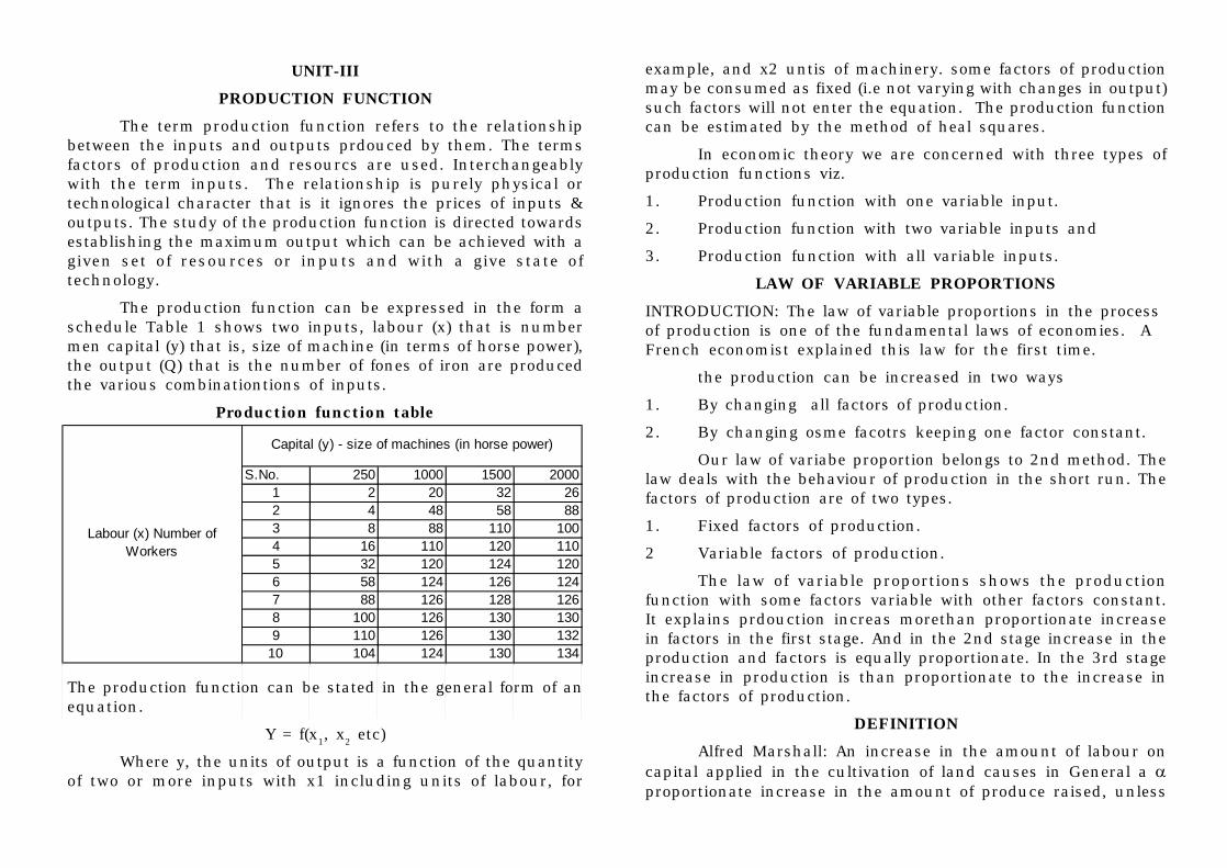
The production function can be expressed in the form aschedule Table 1 shows two inputs, labour (x) that is numbermen capital (y) that is, size of machine (in terms of horse power),the output (Q) that is the number of fones of iron are producedthe various combinationtions of inputs.

Production function table

The production function can be stated in the general form of anequation.

Y = f(x1, x2 etc)

Where y, the units of output is a function of the quantityof two or more inputs with x1 including units of labour, for

S.No. 250 1000 1500 20001 2 20 32 262 4 48 58 883 8 88 110 1004 16 110 120 1105 32 120 124 1206 58 124 126 1247 88 126 128 1268 100 126 130 1309 110 126 130 132

10 104 124 130 134

Capital (y) - size of machines (in horse power)

Labour (x) Number of Workers

example, and x2 untis of machinery. some factors of productionmay be consumed as fixed (i.e not varying with changes in output)such factors will not enter the equation. The production functioncan be estimated by the method of heal squares.

In economic theory we are concerned with three types ofproduction functions viz.

1. Production function with one variable input.

2. Production function with two variable inputs and

3. Production function with all variable inputs.

LAW OF VARIABLE PROPORTIONSINTRODUCTION: The law of variable proportions in the processof production is one of the fundamental laws of economies. AFrench economist explained this law for the first time.

the production can be increased in two ways

1. By changing all factors of production.

2. By changing osme facotrs keeping one factor constant.

Our law of variabe proportion belongs to 2nd method. Thelaw deals with the behaviour of production in the short run. Thefactors of production are of two types.

1. Fixed factors of production.

2 Variable factors of production.

The law of variable proportions shows the productionfunction with some factors variable with other factors constant.It explains prdouction increas morethan proportionate increasein factors in the first stage. And in the 2nd stage increase in theproduction and factors is equally proportionate. In the 3rd stageincrease in production is than proportionate to the increase inthe factors of production.

DEFINITIONAlfred Marshall: An increase in the amount of labour on

capital applied in the cultivation of land causes in General a αproportionate increase in the amount of produce raised, unless

it happens to coincide with the improvement in the arts ofproduction.

Explanation of the law: The law can be explained with the helpof an example of cultivating a limited area of land. If the formergoes on increasing the labour and capital in cultivation of land.That result in 3 stages of output.

1. Increasing returns.

2. Constant returns.

3. Diminishing returns.

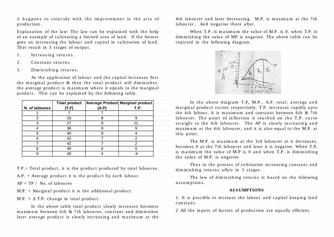
As the application of labour and the capital increases firstthe marginal product & then the total product will diminishes.the average product is maximum where it equals to the marginalproduct. This can be explained by the following table.

T.P.= Total product, it is the product produced by total laboures.

A.P. = Average product it is the product by each labour.

AP = TP / No. of laboures

M.P. = Marginal product it is the additional product.

M.P. = Δ T.P. change in total product.

In the above table total product slowly increases becomesmaximum between 6th & 7th laboures, constant and diminisheslater average product is slowly increasing and maximum at the

N. of labouresTotal product

(T,F)Average Product

(A.P)Marginal product

T.P.1 7 7 -2 16 8 93 27 9 114 36 9 95 40 8 46 42 7 27 42 7 28 40 6 09 36 4 -4

4th labourer and later decreasing. M.P. is maximum at the 7thlabourer. And negative there after.

When T.P. is maximum the value of M.P. is 0. when T.P. isdiminishing the value of MP is negative. The above table can becepicted in the following diagram.

In the above diagram T.P, M.P., A.P. total, average andmarginal product curves respectively. T.P. increases rapidly uptothe 4th labour. It is maximum and constant between 6th & 7thlabourer. The point of inflection it reached on the T.P. curvestraight to the 4th labourer. The AP is slowly increasing andmaximum at the 4th labourer, and it is also equal to the M.P. atthis point.

The M.P. is maximum at the 3rd labourer at it decreases,becomes 0 at the 7th labourer and later it is negative. When T.P.is maximum the value of M.P is 0 and when T.P. is diminishingthe value of M.P. is negative.

Thus in the process of cultivation increasing constant anddiminishing returns affair in 3 stages.

The law of diminishing returns is based on the followingassumptions.

ASSUMPTIONS1. It is possible to increase the labour and capital keeping landconstant.

2 All the inputs of factors of production are equally efficient.

3. There is perfect competition among the factors of production.

4. The factors of production are perfectly among the various uses.

5. The state of technology remains unchanged.

6. This law is applicable only to the short period.

7. the prices of factors of production do not change.

LIMITATIONS OF THE LAWThe law has the following limitations.

1. This law is not applicable to the virgin soil. An increase labourand capital applied in cultivation of virgin soil causes morethanproportionate increase in production.

2. Modern economists believe that where labour and capital areless than the optimum proportion to the land the productivity oflabour & capital may increase.

PRODUCTION ANALYSISIntroduction: Introduction analysis begins with the analysis ofdemand. Once demand for a given prdouct or service has beendetermined, management decides the most profitable way toemploye the firms resources to rpdouce that good or service.Such decisions involve an understandings of what economistscall production function.

A production function is simply or input output relationship.It is analysed and quantified during a production study. Thegoat of production study is to determine the most economicalinput of resources to obtain a given level of output. Or conversely,it involves the determination of the maximum output obtainablefrom a give level and mix of inputs. A production study maypertain not only to the production of goods (such as automobilescalculators, or pet foods) but also to the production of services(such as TV repair, hair styling government assistance & healthcare).

ISO QUANTSProduction function with two variable inputs and laws of

returns.

Let us consider a production process that requires twoinputs capital (C) and labour (L) to produce a given output (Q).there could be morethan two inputs in a real life situation, butfor a simple we production function based on two can be expressedas

Q=f (C,L)

Where C refers to capital L is labour

Normally, both capital and labour are required to producea product. to some extent these two inputs can be substitutedfor each other. Hence the producer may choose any combinationof labour & capital that gives him the required number of unitsof output (see diagram 1) For any given level of output a producermay hire both capital and labour, buthe is free to choose anyone combination of labour and capital out of several suchcombination. The alternative combinations of labour and capitalyielding a given level of output are such that if the use of onefactor input is increased, that of another will decrease and viceversa. However, the units of an input foregone to get one unit ofthe other input charges, depends upon the degree ofsubstitutability, between the input factors. Based on thetechniques or technology used the degree of substitutability mayvary.

ISO Quaris: ISO means equal, quant means quantity - ISO quantmeans that the quantities though at a given ISO Quant are equal.ISO quants are also called ISO prdouct curves. An ISO quantcurve shows various combinations of two inputs factors such ascapital and labour.

As an ISO quant curve represents all such combinationsfor the manufacture. Since he prefers all these combinationsequally, an ISO quant curve is also called product in differencecurve.

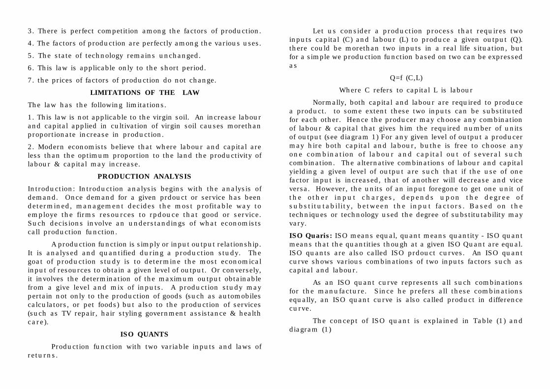
The concept of ISO quant is explained in Table (1) anddiagram (1)

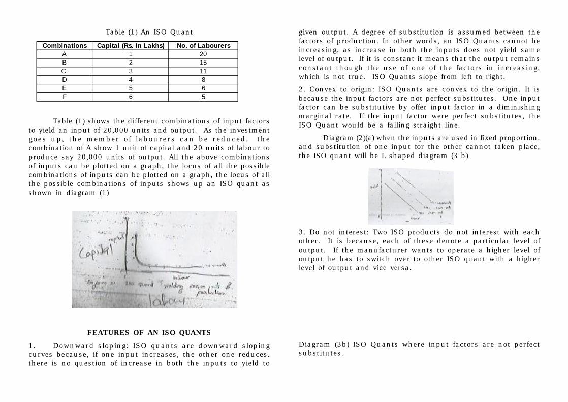
Table (1) An ISO Quant

Table (1) shows the different combinations of input factorsto yield an input of 20,000 units and output. As the investmentgoes up, the member of labourers can be reduced. thecombination of A show 1 unit of capital and 20 units of labour toproduce say 20,000 units of output. All the above combinationsof inputs can be plotted on a graph, the locus of all the possiblecombinations of inputs can be plotted on a graph, the locus of allthe possible combinations of inputs shows up an ISO quant asshown in diagram (1)

FEATURES OF AN ISO QUANTS1. Downward sloping: ISO quants are downward slopingcurves because, if one input increases, the other one reduces.there is no question of increase in both the inputs to yield to

Combinations Capital (Rs. In Lakhs) No. of LabourersA 1 20B 2 15C 3 11D 4 8E 5 6F 6 5

given output. A degree of substitution is assumed between thefactors of production. In other words, an ISO Quants cannot beincreasing, as increase in both the inputs does not yield samelevel of output. If it is constant it means that the output remainsconstant though the use of one of the factors in increasing,which is not true. ISO Quants slope from left to right.

2. Convex to origin: ISO Quants are convex to the origin. It isbecause the input factors are not perfect substitutes. One inputfactor can be substitutive by offer input factor in a diminishingmarginal rate. If the input factor were perfect substitutes, theISO Quant would be a falling straight line.

Diagram (2)(a) when the inputs are used in fixed proportion,and substitution of one input for the other cannot taken place,the ISO quant will be L shaped diagram (3 b)

3. Do not interest: Two ISO products do not interest with eachother. It is because, each of these denote a particular level ofoutput. If the manufacturer wants to operate a higher level ofoutput he has to switch over to other ISO quant with a higherlevel of output and vice versa.

Diagram (3b) ISO Quants where input factors are not perfectsubstitutes.

Do not touch axes: the ISO Quant touches neither X-axis nor Y-axis, as both inputs are required to produce a given product.

COB-DOUGLAS PRODUCTION FUNCTIONCob and Douglas put forth a production function relating

output in America manufacturing industries from 1899 to 1922to labour and capital inputs. they used the following formula.

P=

Where P is the total output.

L is the index of employment of labor in manufacturing.

C is the index of fixed capital in manufacturing.

the exponents a and l-a are the elasticities of prdouction.These measure the percentage response output to percentagechanges in labour and capital respectively.

the function estimated for the USA by Cob and Douglas is

P=1.01L0.75C0.25

R2=0.9409

The production function shows that one percent changein labour input, capital remaining the same, is associated, witha 0.75 percent change in output. Similarly, one percent changein capital, labour remaining the same is associated with a 0.25percent change in output. The coefficient of determination (R2)mean that 94 percent of the variations on the dependent variable(P) were accounted for by the variations in the independentvariables (Land C). It indicates constant returns to scale whichmeans that there smal scale plants are considered equallyprofitable in the US manufacturing industry, on the assumptionthat the average and marginal production costs are constant.

Though Cobb doglas production function was based onmacro-level study, it has been very useful for interpretingeconomic results. Later investigation revealed that the sum ofthe exponents might be very slightly larger than unity, whichimplies decreasing costs, but the difference was so marginalthat constant costs would seem to be a safe assumption for allpractical purposes.

RETURNS TO SCALEThe law of returns to scale explain how a simultaneous

and proportionate increase in all the inputs effects the totaloutput. The increase in output may be proportionate, more thanproporitinate or less than proportionate. If the increase in outputis proportionate to the increase in inputs if it is constant returnsto scale. If is it is few than proportionate it is diminishing returnsto scale. the increasing returns to scale comes in operation firstthen constant and then diminishing returns to scale, and it wasshown in the diagram.

1) Increasing returns to Scale Increasing returns to scale is thestage of production when a proportionate increase in all factorsof production. Results in a more than proportionable increase inoutput. It s the first stage of production. The marginal outputincreases at this stage. The increase in efficiency resulting inincreased output in due to the better utilisation of plant or higherdegree of specialisation. The factors of production which arealready in use may be some indivisible unis. the nature ofproduction in such that large investments must be made in theseindivisible units before production starts.

The increase returns may be due to the increased

specialisation. Increase in output helps to adopt higher scale ofspecialisation leading to increased efficiency and falling costs.It may be now able to use large and expensive machines, andthe services of experts or of highly skilled labour which willresult in fall in marginal cost.

2. Constant Returns to scale. The increasing returns to scalestage will not continue indefinitely. The firm gradually loosesall those economies of prdouction. Now the firm enters a stageat which total output tends to increase at a rate which is equalto the rate of increase in inputs. That is when the inputs aredoubled it results in a doubling of output. This stage comes tooperation. When the economies of large scale production areneutralized by the diseconomies of large scale operation.

3. Diminishing Returns to scale: If the firm continues to expandbeyond the stage of constant returns, the stage of diminishingreturns to scale starts operating. A proportionate increase inall the inputs in this stage results only in a less than proportionateincrease in output. This is because of the diseconomies of largescale production. When a firm grows in size beyond a certainscale the management becomes difficult. Thus inefficiency ceepsin.

ECONOMICS OF LARGE SCALE PRODUCTIONWhen a firm increase all the factors of production of enjoys

some advantage of economies of production. The economies ofscale are classified as:

1. Internal economies and

2. External economies

Internal economies: Internal economies are economieswhere are available to a particular firm and this will be differentfor different firms. This is due to the expansion of the size ofthe firm. Internal economies may be classified as

a) Technical economies: A large size firm can afford right type ofmachinery or various specialized machineries. A small firmcannot afford modern highly specialized machines and the

advantages of modern advanced technology. Though itsinstallation involve high cost, ithelps to bring out more output ofa lesser cast thus reducing the cost per unit.

b) Labour Economies: When the firm expands its scale operationit absorbs more and more workers with different qualifications.Thus these workers can be divided according to their qualificationand skill and be placed of the proper operations.

c) Managerial economies: A large size firm can employ speciallyqualified persons to look after various sections like, production,financing, marketing, personnel etc. This specialization inmanagerial staff increases the efficiency of management.Moreover the sales co-ordination through wholesale wil be moreeffective and les scheap.

d) Marketing economies: The large size firm can make bulk-purchases of raw materials etc. at better terms. If can enjoythe discount on bulk purchasing which smaller firms cannotenjoy. It can appoint exprt buyers and expert salesman. It cansecure the economies of large scale selling.

e) Economies in Transprot and Storage: The large size form canafford its own transportation system. This helps to reduce thetransportation cost and avoid delay in transportation large scalefirms ca keep their own godowns in various centers thus reducingthe sstorage cost.

2. External economies: An individual firm is not responsible forthis when may firms in an industry expand in a particular areathey all may share in same advantages. The expansion of all thefirms in region may make possible the development of transportand communication of that region. Cheaper systems oftransportation like railway may be introduced.

UNIT-IIIPROFIT

Introduction: In common parlance profit means the net incomeof a businessman. It is calculated by deduction from the totalreceipts. The total expenditure incurred in a business venture.But profit is the above sense is not the something as defined byeconomists. Economists regard profit as a factor-return likewages, interest and rent to them profit is a return to theentrepreneur for the use of his entrepreneurial ability. It becomesimportant to know what we mean by return for entrepreneurialability. Since the return for his routine management is wages,he must do something other than routine management to earnprofit essential there are two things an entrepreneur does:

1. He divides when where and how he is to use his limitedresources. He also plans how much quality of inputs he is to usefor production. Each of these decisions is taken at a movementof time, but there certainly govern the future. Conduct andperformance of business.

2. His second job is that of innovation. In attempting to makeprofit the entrepreneur must search around for new methods ofproduction, new ways of business organisation, new marketingtechnique and approaches and the like.

MEASUREMENT OF PROFITEconomic profit is quite different from accounting profit

economic profit includes opportunity cast, which is not easilyidentifiable a measurable on the other hand, the accountingcosts, both direct and indirect are easily identified and recorded.There are three specific aspects of profit measurements wherethe use of accounting profit and of economic profit give differentresults.

1. Depreciation: An accountant measures the cost ofdepreciation by several methods like, straight line method,diminishing-balance method, Annuity method, service unitmethod. For economist these methods are of mouse. He looksat depreciation in terms of opportunity costs and uses the asset

replacement costs rather than the original or historical costs ofthe assets. The replacement investment is needed to keep capitalstock intact. The opportunity costs of not taking timelyreplacement increasing level and rate of depreciation andobsolescence.

2. Inventory Valuation: This is another area of profitmeasurement where accounting conventions and economicconcepts give different results. Inventory or stocks refer to goodsin pipe line - difference between production and consumption.When production exceeds consumption, the stocks file up. Suchinventory building or stock filling would have posted no problemsof valuations, had prices remain stable, materials costs changeand therefore the valuation of stocks must change. Theaccountant uses some standard methods viz. FIFO, LIFO weightedaverage etc. The economists feels that recorded value of businessincome in different periods may differ considerably, dependingupon, the methods of valuation chosen. For above measure ofvaluation the net business income should be measured atconstant prices.

3. Unaccounted value changes: There may be certain items ofbusiness expenditure which may not have any impact on currentbusiness income, but which may in case future income of thefirm. The accountant does not consider the future value of thepresent expenditure on items like Research and Development,advertisement requirement of skillful managers etc. In theprocess the accountant may undertake current profit andoverstate future profit.

PROFIT MAXIMIZATION Vs WEALTH MAXIMIZATIONAs we know that profit maximization is fundamental

objective of the business. Wealth maximization also one of theobjectives of the business firm. Accumulated profits can beconverted into sales maximization or wealth maximization. Ifthe advertisement expenditures is increased, then it will helpin increase of sales. If profits are converted into reserves, orpurchase of new equipment or purchase of new machinery, itwill be leading to wealth maximization. Any businessman wants

to rise in wealth of business showever if he neglects salesmaximization then it will hamper success of business.

Profit maximization is also depends on the achievementof sales targets. To achieve the expected targets, business firmswill try to attract consumers by offering discounts, free gifts,bundle-pack offers etc. Sometimes prices may be reduced for acertain period of time to increase sales. In such cases, profitsmay to be declined, however the firms will be able to competewith the rivals and elimination of rivals can be possible bypracticing various sales strategies.

Wealth maximization depends on investment decisions ofthe business. By taking best projects with the help of capitalbudgeting techniques like net present value method or internalrate of return, the firm maximizes its value of investment. Thehigher returns will give higher value to the organisation. Thevalue of firm is also depends upon goodwill, quality of the product,and social commit of the firm. Hence every business firm aimsto achieve value of wealth maximization as well as profitmaximization.

Equations: Profit = Total revenue - total cost

TR = TC

Profit maximization:

MR- MC

dQdTRMR = differentiating revenue / cast function

dQdTCMC ==

dQdTC

dQdTRP −=

WHAT IS COSTThe expenditure incurred on manufacturing a product i.e.

material, labour and other overhead is called “cost” of thatparticular product mathematically cost function can be writtenas:

C = f(d,T,PF,K)

C = Total cost

X = output

T = Technology

PF = Price of factors

K = Fixed cost

Elements of cost:

a) Prime cost: Direct materials + Director labour + Directexpenses.

b) Factory cost: Prime cost + Factory expenses

c) Cost of production: Factory cost + administration expenses.

d) Total Cost : Cost of production + selling and distributionexpenses.

Definition of cost:

1. Cost is a measurement in monetary terms of the amount ofresources used for some purpose. Anthony & Wegen.

2. The foregoing in monetary terms, incurred or potentially to beincurred in the realization of the objective of management whichmay be manufacturing of a product of rendering of a service >committee on cost terminology of American Accountingassociation.

COST OUTPUT RELATIONSHIPThe concept of cost analysis is has a great significance in

modern business world. Every business firm has to forecast. Hefuture cost conditions so as to determined the optimum outputand adopt an appropriate price policy. The theories of production

are also based on the analysis of costs.

Procedures aim to achieve maximum output at minimumof cast. The relationship between cast and output enables theproducer to study the quantity of cast a various levels of output.The cost analysis and its study is conducive (helpful) to fix thequantity of output at maximum cast of production procedure hasto study the relation between cost and output so as to co-ordinatethe factors of production in an optimum manner.

The relation between cast and output is of two types.

1. Short run relation.

2. Long run relation.

1. Short run relation: In the short run the costs are divided intotwo types.

a) Fixed costs.

b) Variable costs.

The fixed factors of production are constant and onlyvariable functions change in the short run. In this period thefirm does not have enough time to change its scale of operationshence the costs decrease and increase very rapidly in this period.The variable cost curves are completely. “U” shaped.

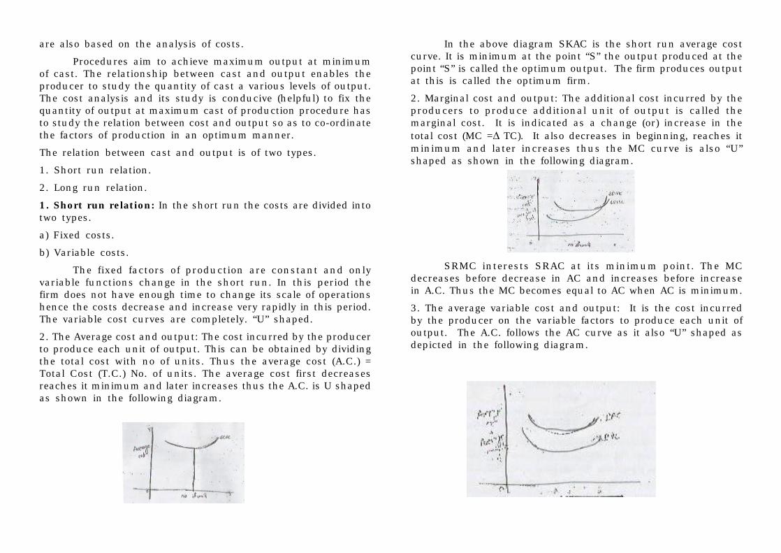
2. The Average cost and output: The cost incurred by the producerto produce each unit of output. This can be obtained by dividingthe total cost with no of units. Thus the average cost (A.C.) =Total Cost (T.C.) No. of units. The average cost first decreasesreaches it minimum and later increases thus the A.C. is U shapedas shown in the following diagram.

In the above diagram SKAC is the short run average costcurve. It is minimum at the point “S” the output produced at thepoint “S” is called the optimum output. The firm produces outputat this is called the optimum firm.

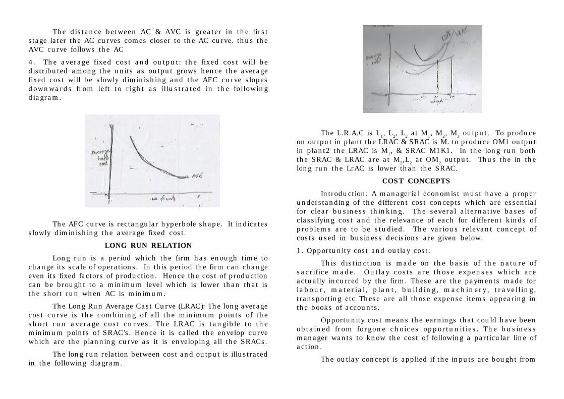
2. Marginal cost and output: The additional cost incurred by theproducers to produce additional unit of output is called themarginal cost. It is indicated as a change (or) increase in thetotal cost (MC =Δ TC). It also decreases in beginning, reaches itminimum and later increases thus the MC curve is also “U”shaped as shown in the following diagram.

SRMC interests SRAC at its minimum point. The MCdecreases before decrease in AC and increases before increasein A.C. Thus the MC becomes equal to AC when AC is minimum.

3. The average variable cost and output: It is the cost incurredby the producer on the variable factors to produce each unit ofoutput. The A.C. follows the AC curve as it also “U” shaped asdepicted in the following diagram.

The distance between AC & AVC is greater in the firststage later the AC curves comes closer to the AC curve. thus theAVC curve follows the AC

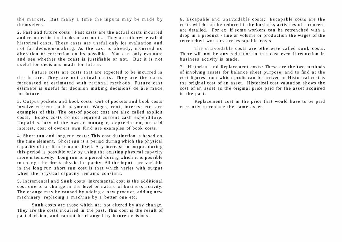
4. The average fixed cost and output: the fixed cost will bedistributed among the units as output grows hence the averagefixed cost will be slowly diminishing and the AFC curve slopesdownwards from left to right as illustrated in the followingdiagram.

The AFC curve is rectangular hyperbole shape. It indicatesslowly diminishing the average fixed cost.

LONG RUN RELATIONLong run is a period which the firm has enough time to

change its scale of operations. In this period the firm can changeeven its fixed factors of production. Hence the cost of productioncan be brought to a minimum level which is lower than that isthe short run when AC is minimum.

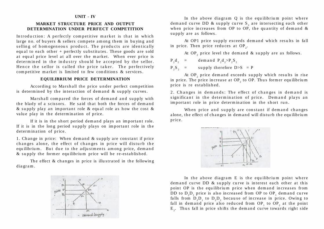
The Long Run Average Cast Curve (LRAC): The long averagecost curve is the combining of all the minimum points of theshort run average cost curves. The LRAC is tangible to theminimum points of SRAC’s. Hence it is called the envelop curvewhich are the planning curve as it is enveloping all the SRACs.

The long run relation between cost and output is illustratedin the following diagram.

The L.R.A.C is L1, L2, L2 at M1, M2, M3 output. To produceon output in plant the LRAC & SRAC is M. to produce OM1 outputin plant2 the LRAC is M1, & SRAC M1K1. In the long run boththe SRAC & LRAC are at M2,L2 at OM2 output. Thus the in thelong run the LrAC is lower than the SRAC.

COST CONCEPTSIntroduction: A managerial economist must have a proper

understanding of the different cost concepts which are essentialfor clear business thinking. The several alternative bases ofclassifying cost and the relevance of each for different kinds ofproblems are to be studied. The various relevant concept ofcosts used in business decisions are given below.

1. Opportunity cost and outlay cost:

This distinction is made on the basis of the nature ofsacrifice made. Outlay costs are those expenses which areactually incurred by the firm. These are the payments made forlabour, material, plant, building, machinery, travelling,transporting etc These are all those expense items appearing inthe books of accounts.

Opportunity cost means the earnings that could have beenobtained from forgone choices opportunities. The businessmanager wants to know the cost of following a particular line ofaction.

The outlay concept is applied if the inputs are bought from

the market. But many a time the inputs may be made bythemselves.

2. Past and future costs: Past casts are the actual casts incurredand recorded in the books of accounts. They are otherwise calledhistorical casts. These casts are useful only for evaluation andnot for decision-making. As the cast is already, incurred noalteration or correction on its possible. You can only evaluateand see whether the coast is justifiable or not. But it is notuseful for decisions made for future.

Future costs are costs that are expected to be incurred inthe future. They are not actual casts. They are the castsforecasted or estimated with rational methods. Future castestimate is useful for decision making decisions de are madefor future.

3. Output pockets and book costs: Out of pockets and book costsinvolve current cash payment. Wages, rent, interest etc. areexamples of this. The out-of pocket cost are also called explicitcosts. Books costs do not required current cash expenditure.Unpaid salary of the owner manager, depreciation, unpaidinterest, cost of owners own fund are examples of book costs.

4. Short run and long run costs: This cost distinction is based onthe time element. Short run is a period during which the physicalcapacity of the firm remains fixed. Any increase in output duringthis period is possible only by using the existing physical capacitymore intensively. Long run is a period during which it is possibleto change the firm’s physical capacity. All the inputs are variablein the long run short run cost is that which varies with outputwhen the physical capacity remains constant.

5. Incremental and Sunk costs: Incremental cost is the additionalcost due to a change in the level or nature of business activity.The change may be caused by adding a new product, adding newmachinery, replacing a machine by a better one etc.

Sunk costs are those which are not altered by any change.They are the costs incurred in the past. This cost is the result ofpast decision, and cannot be changed by future decisions.

6. Escapable and unavoidable costs: Escapable costs are thecosts which can be reduced if the business activities of a concernare detailed. For ex: if some workers can be retrenched with adrop in a product - line or volume or production the wages of theretrenched workers are escapable costs.

The unavoidable costs are otherwise called sunk costs.There will not be any reduction in this cost even if reduction inbusiness activity is made.

7. Historical and Replacement costs: These are the two methodsof involving assets for balance sheet purpose, and to find at thecost figures from which profit can be arrived at Historical cost isthe original cost of an asset. Historical cost valuation shows thecost of an asset as the original price paid for the asset acquiredin the past.

Replacement cost in the price that would have to be paidcurrently to replace the same asset.

UNIT - IVMARKET STRUCTURE PRICE AND OUTPUT

DETERMINATION UNDER PERFECT COMPETITIONIntroduction: A perfectly competitive market is that in whichlarge no. of buyers & sellers compete among them in buying andselling of homogeneous product. The products are identicallyequal to each other + perfectly substitutes. These goods are soldat equal price level at all over the market. When ever price isdetermined in the industry should be accepted by the sellor.Hence the sellor is called the price taker. The perfectivelycompetitive market is limited to few conditions & services.

EQUILIBRIUM PRICE DETERMINATIONAccording to Marshall the price under perfect competition

is determined by the interaction of demand & supply curves.

Marshall compared the forces of demand and supply withthe blady of a scissors. He said that both the forces of demand& supply play an important role & equal role as how the cost &value play in the determination of price.

If it is in the short period demand plays an important role.If it is in the long period supply plays on important role in thedetermination of price.

1. Change in price: When demand & supply are constant if pricechanges alone, the effect of changes in price will disturb theequilibrium. But due to the adjustments among price, demand& supply the former equilibrium price will be re-established.

The effect & changes in price is illustrated in the followingdiagram.

In the above diagram Q is the equilibrium point wheredemand curve DD & supply curve S3 are intersecting each otherwhen price increases from OP to OP, the quantity of demand &supply are as follows.

At OP1 price supply exceeds demand which results in fallin price. Then price reduces at OP2.

At OP2 price level the demand & supply are as follows.

P2d2 = demand P2d2>P2S2

P2S2 = supply therefore D>S = P

At OP2 price demand exceeds supply which results in risein price. The price increase at OP2 to OP. Thus former equilibriumprice is re established.

2. Changes in demands: The effect of changes in demand issignificant in the determination of price. Demand plays animportant role in price determination in the short run.

When price and supply are constant if demand changesalone, the effect of changes in demand will disturb the equilibriumprice.

In the above diagram E is the equilibrium point wheredemand curve DD & supply curve is interest each other at thispoint OP is the equilibrium price when demand increases fromDD to D2D1 price is also increased from OP to OP1 demand curvefalls from D2D1 to D2D2 because of increase in price. Owing tofall in demand price also reduced from OP1 to OP2 at the pointE2. Thus fall in price shifts the demand curve towards right side

again at the point-E former equilibrium price OP is reestablished.

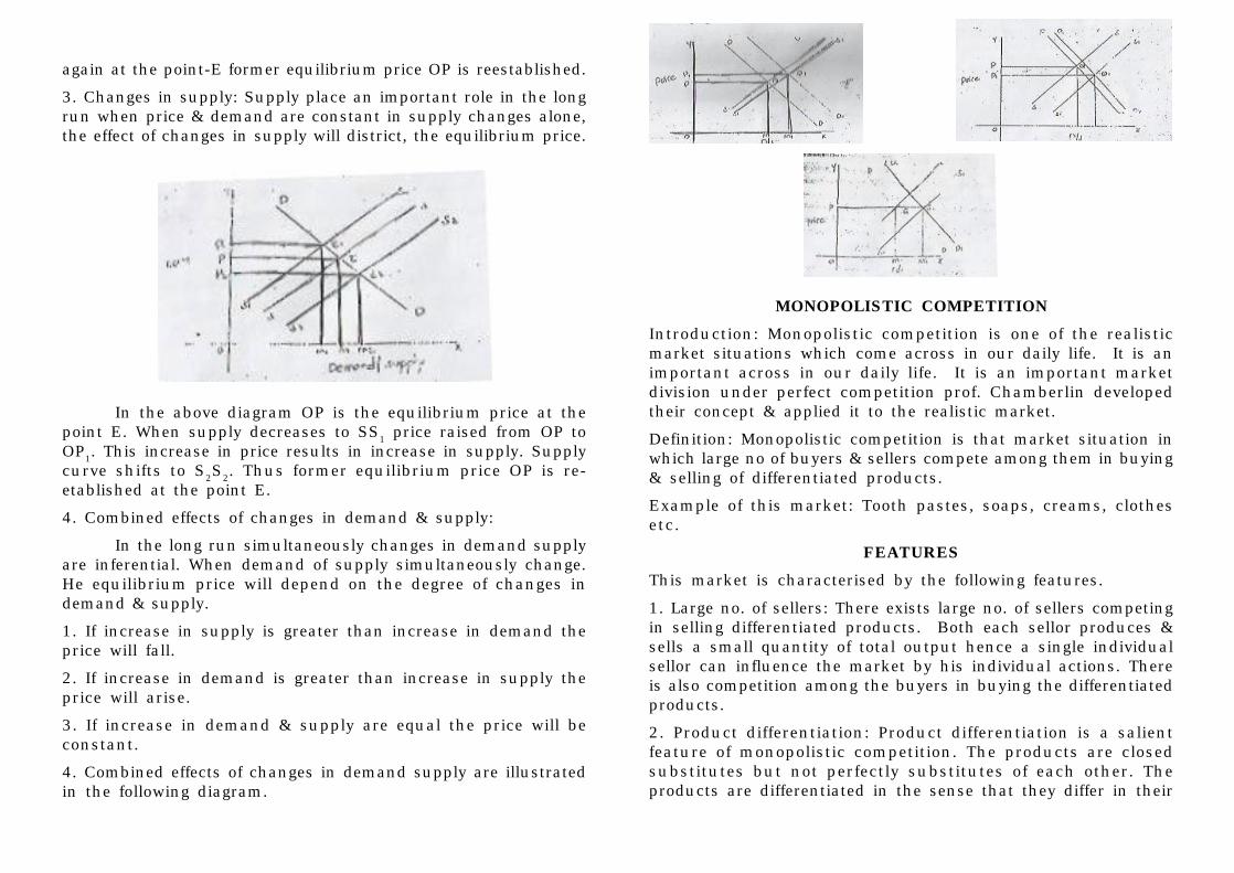
3. Changes in supply: Supply place an important role in the longrun when price & demand are constant in supply changes alone,the effect of changes in supply will district, the equilibrium price.

In the above diagram OP is the equilibrium price at thepoint E. When supply decreases to SS1 price raised from OP toOP1. This increase in price results in increase in supply. Supplycurve shifts to S2S2. Thus former equilibrium price OP is re-etablished at the point E.

4. Combined effects of changes in demand & supply:

In the long run simultaneously changes in demand supplyare inferential. When demand of supply simultaneously change.He equilibrium price will depend on the degree of changes indemand & supply.

1. If increase in supply is greater than increase in demand theprice will fall.

2. If increase in demand is greater than increase in supply theprice will arise.

3. If increase in demand & supply are equal the price will beconstant.

4. Combined effects of changes in demand supply are illustratedin the following diagram.

MONOPOLISTIC COMPETITIONIntroduction: Monopolistic competition is one of the realisticmarket situations which come across in our daily life. It is animportant across in our daily life. It is an important marketdivision under perfect competition prof. Chamberlin developedtheir concept & applied it to the realistic market.

Definition: Monopolistic competition is that market situation inwhich large no of buyers & sellers compete among them in buying& selling of differentiated products.

Example of this market: Tooth pastes, soaps, creams, clothesetc.

FEATURESThis market is characterised by the following features.

1. Large no. of sellers: There exists large no. of sellers competingin selling differentiated products. Both each sellor produces &sells a small quantity of total output hence a single individualsellor can influence the market by his individual actions. Thereis also competition among the buyers in buying the differentiatedproducts.

2. Product differentiation: Product differentiation is a salientfeature of monopolistic competition. The products are closedsubstitutes but not perfectly substitutes of each other. Theproducts are differentiated in the sense that they differ in their

quality, quantity, price, fragrance, physical appearance,workmanship, longevity etc. The product differentiation is byadopting copy rights, patent rights & other techniques the firmsregister their brand names, chemical combinations, designs &packaging.

3. Free entry exists of firms: The firms are free to enter or leavethe group. When the group of firms enjoys abnormal profits newfirms enter the group similarly if the group is suffering fromlosses the existing firms may leave the group. The process ofentry exists of firms is applicable only in the long run.

4. Independent price policy: Each firm outputs its own price policyon the basis of demand for its product. Firms consider the costof production market demand companies reputation whiledetermining the price. In this case cast plus pricing, skimmingup pricing, penetration price policy are some of the policiesadopted by the firms.

5. Selling cost: The cost of selling cost was introduced by proofchamberlain. According to him selling cost are those costs whichare incurred by the firm in order to alter the shape of the demandcurve. The costs are in the firm of advertisements, free giftsincentives, lucky coupons etc.

6. Market imperfections: Monopolistic competition ischaracterised by market imperfections both the buyers & sellersdo not have complete knowledge about the market conditions.The buyers & sellers do not have knowledge on price, supply ofdemand for the substitutes in the market.

7. Imperfect Mobility of factors: The factors of production areperfectly mobile among various uses. The factors will stick onthe existing group without changing their palace, process ofproduction etc.Similarly the prices of factors of production aredifferent from each other. An efficient unit of factors can earnmax than what the other factors remuneration.

EQUILIBRIUM PRICE OUTPUT DETERMINATIONEquilibrium is said to exist when a firm does not have any

tendency to change its output. A fir, at its equilibrium, earns

maximum profits where its marginal cost is equal to its marginalrevenue.

The firm reaches its equilibrium where the MC is equal toMR & MC curve interesects the MR from below only.

The group of firms, under monopolistic, is not called theindustry because the firms produce the differentiated products.Hence all the firms in the market are combinedly called thegroup.

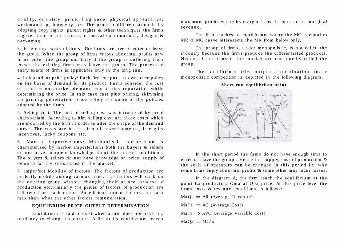
The equilibrium price output determination undermonopolistic competition is depicted in the following diagram.

Short run equilibrium point

In the short period the firms do not have enough time toenter or leave the group. Hence the supply, cost of production &the scale of operators can be changed in this period i.e. whysome firms enjoy abnormal profits & some other may incur losses.

In the diagram A, the firm reach the equilibrium at thepoint Ea producting Oma at Opa price. At this price level thefirms costs & revenue conditions as follows:

MaQa ⇒ AR (Average Revenue)

MaJa ⇒ AC (Average Cost)

MaTa ⇒ AVC (Average Variable cost)

MaQa ⇒ MaJa

Therefore AR>AC & AVC

QaSa = Profit per unit

PaQaSaRa = Total profit OMa output.

On the diagram B “EB” is the equilibrium point of the firmproducing OMb output at 6 OPb price at this price level the firmscosts & Revenue condition are as follows:

MbQb = AR & AVC

Mb Sb = AC

Mb Sb > Mbab

Therefore AC>AR

Sb Qb = loss of each unit

Pb Qb Sb Rb = total loss area of the firm B on Omb output.

LONG RUN EQUILIBRIUMLong run is the period in which the period firms have

enough time to enter (or) leave the group supply can be adjustedto the extend of changer in demand & price hence all the firmsin the long run, earn normal profits only.

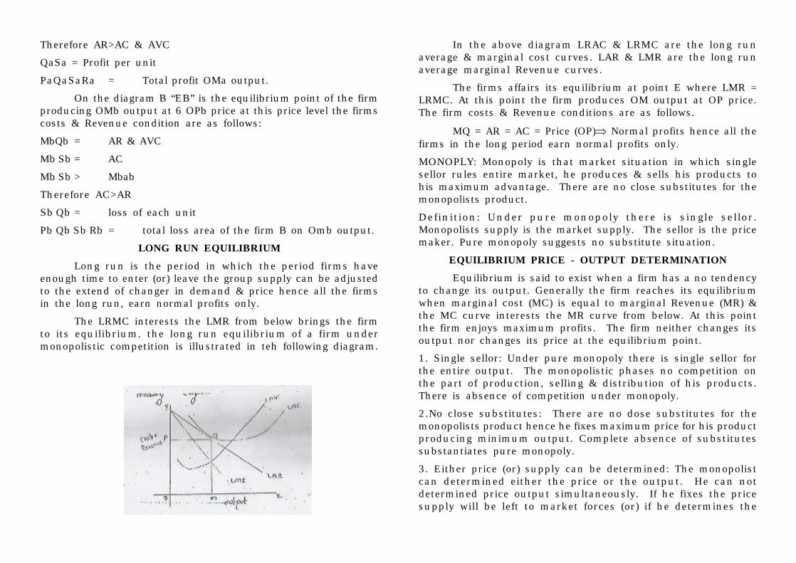
The LRMC interests the LMR from below brings the firmto its equilibrium. the long run equilibrium of a firm undermonopolistic competition is illustrated in teh following diagram.

In the above diagram LRAC & LRMC are the long runaverage & marginal cost curves. LAR & LMR are the long runaverage marginal Revenue curves.

The firms affairs its equilibrium at point E where LMR =LRMC. At this point the firm produces OM output at OP price.The firm costs & Revenue conditions are as follows.

MQ = AR = AC = Price (OP)⇒ Normal profits hence all thefirms in the long period earn normal profits only.

MONOPLY: Monopoly is that market situation in which singlesellor rules entire market, he produces & sells his products tohis maximum advantage. There are no close substitutes for themonopolists product.

Definition: Under pure monopoly there is single sellor.Monopolists supply is the market supply. The sellor is the pricemaker. Pure monopoly suggests no substitute situation.

EQUILIBRIUM PRICE - OUTPUT DETERMINATIONEquilibrium is said to exist when a firm has a no tendency

to change its output. Generally the firm reaches its equilibriumwhen marginal cost (MC) is equal to marginal Revenue (MR) &the MC curve interests the MR curve from below. At this pointthe firm enjoys maximum profits. The firm neither changes itsoutput nor changes its price at the equilibrium point.

1. Single sellor: Under pure monopoly there is single sellor forthe entire output. The monopolistic phases no competition onthe part of production, selling & distribution of his products.There is absence of competition under monopoly.

2.No close substitutes: There are no dose substitutes for themonopolists product hence he fixes maximum price for his productproducing minimum output. Complete absence of substitutessubstantiates pure monopoly.

3. Either price (or) supply can be determined: The monopolistcan determined either the price or the output. He can notdetermined price output simultaneously. If he fixes the pricesupply will be left to market forces (or) if he determines the

supply price will be determined by the market forces.

4. No difference between firm & industry: The entire supplyavailable in the market belongs to a single sellor thissubstantiates that the industry output is equal to the firms output.Hence there is no difference between the firm and industry.

5. Price discrimination: The concept of price discrimination wasintroduced by Mrs. Jagan Robbinson according to her. An art ofselling the same article at different prices, at different markets,to the different buyers is known as price discrimination.

Only monopoly can participate in price discrimination byintroducing differences in fixed ability of his products. He adoptsthis technique on the basis differences in the elasticity of demandfor his product.

6. Relatively in elastic demand (AR >MR): The monopolistic facesa determinate demand curve which is sleep down words fromleft to right. As the sellor has to decrease the price to selladditional unit increases in total revenue & marginal revenuewith fall. Hence the AR is greater than the MR.

EQUILIBRIUM PRICE - OUTPUT DETERMINATIONEquilibrium is said to exist when a firm has no tendency

to change its output. Generally the firm reaches its equilibriumwhere marginal cost (MC) is equal to marginal revenue (MR) &the MC curve intersects the MR curve from below. At this pointthe firm enjoys maximum profits. The firm neither changes itsoutput nor changes its price at the equilibrium point.

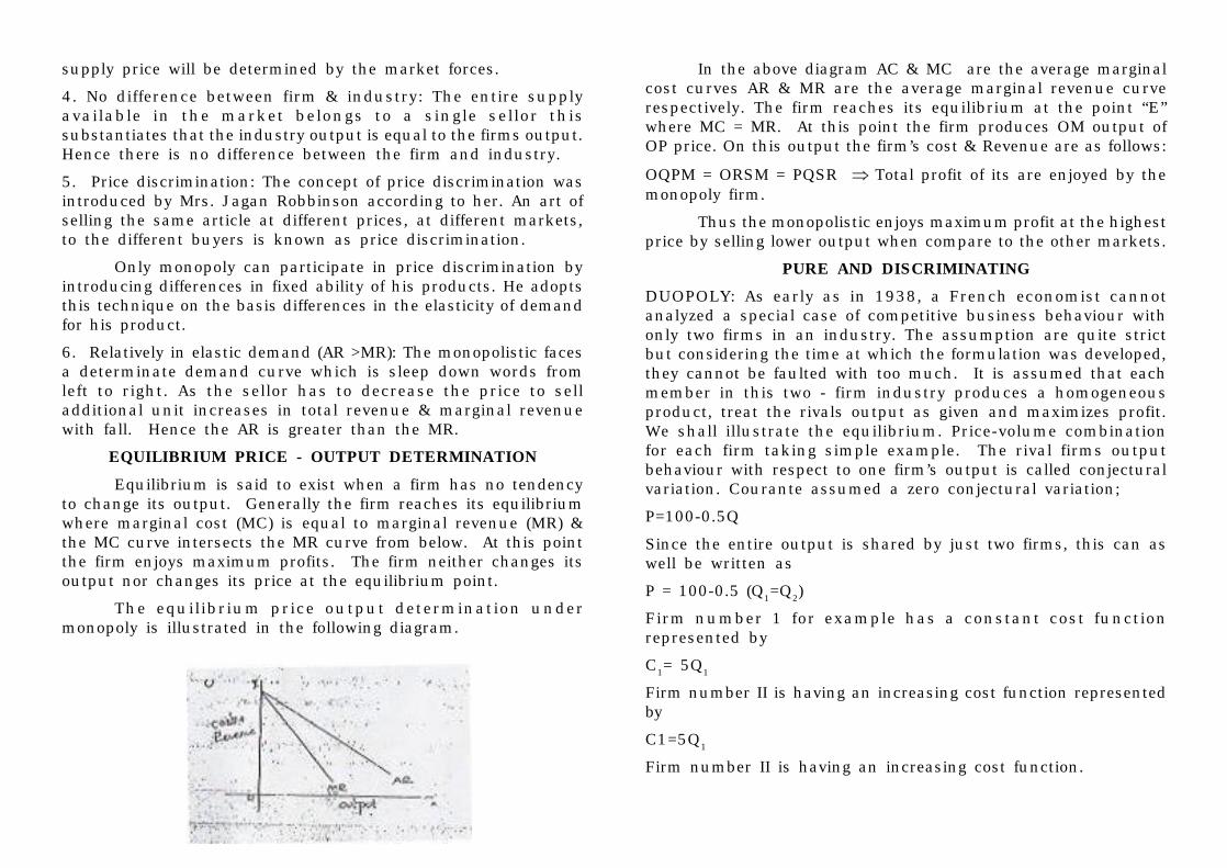
The equilibrium price output determination undermonopoly is illustrated in the following diagram.

In the above diagram AC & MC are the average marginalcost curves AR & MR are the average marginal revenue curverespectively. The firm reaches its equilibrium at the point “E”where MC = MR. At this point the firm produces OM output ofOP price. On this output the firm’s cost & Revenue are as follows:

OQPM = ORSM = PQSR ⇒ Total profit of its are enjoyed by themonopoly firm.

Thus the monopolistic enjoys maximum profit at the highestprice by selling lower output when compare to the other markets.

PURE AND DISCRIMINATINGDUOPOLY: As early as in 1938, a French economist cannotanalyzed a special case of competitive business behaviour withonly two firms in an industry. The assumption are quite strictbut considering the time at which the formulation was developed,they cannot be faulted with too much. It is assumed that eachmember in this two - firm industry produces a homogeneousproduct, treat the rivals output as given and maximizes profit.We shall illustrate the equilibrium. Price-volume combinationfor each firm taking simple example. The rival firms outputbehaviour with respect to one firm’s output is called conjecturalvariation. Courante assumed a zero conjectural variation;

P=100-0.5Q

Since the entire output is shared by just two firms, this can aswell be written as

P = 100-0.5 (Q1=Q2)

Firm number 1 for example has a constant cost functionrepresented by

C1= 5Q1

Firm number II is having an increasing cost function representedby

C1=5Q1

Firm number II is having an increasing cost function.

C2 = 0.5Q22

Firm 1’ s profit = Total revenue- total costs.

= PQ1- 5Q1

= (100-0.5 (Q1+Q2)(Q1-5Q1)

=95Q1 - 0.5Q12-0.5 Q1Q2

The solution of a duopoly equilibrium crucially dependson the nature of the reaction function of each duopolist. Theequilibrium is reached when the values of Q1 and Q2 are such,that each firm maximizes its profit, given the output of the otherand neither desire to alter the respective output. However for acommon solution, both the firms must achieve maximum profitsand the same time have no incentive for changing respectiveoutput levels. Such a solution is obtained at the interesectionpoint of two liner reaction functions.

OLIGOPOLYIntroduction: When only a few sellers of a product are found inthe market it called oligopoly. It is competition among a fewsellers, each selling either differentiated or homogeneousproducts. The term a few sellers implies a number small enoughto enable an individual firm to influence the market price. Eachsellor commands a sizeable preparation of the total market supply.The basic characteristic of an oligopolistic situation is the factthat every sellor can exercise an important influence on theprice - output policies of his rivals.

The products sold by the oligopolist may be differentiatedor homogeneous. If they sells homogeneous product, it is knownas perfect oligopoly, and if they dela with differentiated products,it is known as imperfect oligopoly compared with perfectcompetition, the number of oligopoly is much smaller. Oligopolydiffers from monopoly and monopolistic competition.

CHARACTERISTICS OF OLIGOPOLYThe main features of oligopoly are:

1. Fe firms: there are only a few firms in the industry. Each firm

contributes a sizeable shares of the total market. Any decisiontaken by one firm influences the actions of other firms in theindustry. The various firms in the industry compete with eachother.

2. Interdependence. As there are only few firms any steps takenby one firm to increase sales, by reducing price or by changingproduct design or by increasing advertisement expenditure willnaturally effect the sale of other limits in the industry.

3. Indeterminate demand curve: The interdependence of thefirms make their demand curve indeterminate. Who one firmreduces price other forms also will make a cut in their prices.So the firm cannot be certain about the demand for its product.

4. Advertising and selling costs: Advertising plays a greater rolein the oligopoly market when compared to other market systems.According to prof. William J. Beumol it is only under digopolythat advertising comes fully into the own”.

5. Price rigidity: In the oligopoly market price remains rigid. Ifone firm reduces price it is with the intention of attracting theconsumers of other firms in the industry.

METHODS OF PRICINGIntroduction: A firm is to take into consideration the priceelasticity of a product in fixing its price. If the demand for theproduct is inelastic the management can increase its price andincrease the profit. As the demand in elastic an increase inprice will not decrease the present demand.

1. Cost-plus pricing: This is very common method of determiningthe selling prices of products. It is also know as average costpricing or full cost pricing or margin pricing or markup pricingThe selling price is found out by adding a certain percentagemarkup to the average variable cost. The markup contributionmargin contributes towards fixed cost and profit.

Price = AVC + CM

Suppose the variable cost per unit (AVC) is Rs.8. Themanagement decides to have markup of 25%. Then Rs.2 is the

markup or margin. This is Rs.2 per unit contributes towardsfixed cost and profit.

P = AVC + CM

= 8+2

= Rs. 10

This method of pricing helps to cover the total cost and toensure ‘fair’ profit percentage. Here, cost is the important factorin fixing the price of a product and the demand aspect is takeninto consideration.

DEFECTS OF THIS SYSTEM:1.It ignores the influence of demand on price. There is essentiallyno relationship between cost and what people will be ready topay for a product.

2.The market price and competition are not adequate taken intoconsideration.

3. Here cost is considered as the main factor influencing price.

4. The cost concept made use for ascertaining cost may not berelevant for pricing decisions.

Advantages:1. It helps in fixing a fair price.

2. It can be applied easily.

3. This method is of very much help when the firm is uncertainabout demand.

4. This method of pricing does not postpone the recovery of fixedcosts. The total costs curves both fixed and variable costs.

MARGINAL COST PRICINGIntroduction: Under the marginal cost pricing the price of aproduct is determined on the basis of marginal or variable costand the fixed costs are not considered fixed costs are the resultsof past decisions and hence fixed costs are historical and sunkcosts. This past cost has little relevance in pricing as pricing

decision, involves planning into the future.

Merits:

1. This method is more useful when the demand conditions areslack.

2. The price determined on the basis of this method is morecompetitive.

3. Marginal cost concept helps to ascertain the changes in costdue to a pricing decision.

4. When compared to the full cost pricing marginal cost pricinghelps to adopt a more aggressive pricing policy.

Limitations:1. an accountant who is not fully conversant with the marginalcosting technique finds it difficult to apply this.

2. In a period of business decision the firms applying this methodmay reduce the price the price which will call other competitivefirms also to reduce their prices.

DIFFERENTIAL PRICING:a.Skimming: When a new product is introduced in the market,the firm fixes a price much higher than the cost of production.This consumers are ready to pay a high price to enjoy the pleasureof being the first users of the product. The high price charged toskin the cream off the market at a time when there is nocompetition. This is possible because the newly introducedproduct reached. The hands of the consumers after a long waitingand by the time it comes to the market a heavy demand for thesame as accumulated.

The firm makes a huge profit by price skimming. The priceskimming policy is followed as long as there is heavy demandwithout any competition from a rival. The principle behind priceskimming is to make hay while sun shines.

Under the following situations the price skimming policycan be easily followed.

1. The new product is a novel item which can attract customers

and is having no competitors at present.

2. The product is meant for the higher income group whosedemand is inelastic.

a) There are heavy initial promotion expenses and firm wants torealize it from the customers before other competitive firms enter

The firm, after squeezing the enthusiastic buyers, goes onreducing the price step by step so that it can reach the varioussections of consumers who are willing to buy it at lower prices.

b) Penetration: The fixed price is relatively a lower one. thispricing is resorted to when the new product faces a strongcompetition from the existing substitute products. When thenew firm enters an existing market where there are a numberof firms to has to penetrate the market and achieve an acceptancefor its product. In order to atain this it will charge only a verylow price initially, hoping to charge a normal price later when itis established in the market. For example firm may, when itintroduce a new batch soap in the market, give a 100 gramspiece free when consumers buy two 200 grams pieces at a time.Later when it picks up scales it takes out the initial discount.In a foreign market a new country may have to penetrate.Through a highly competitive price.

The penetration price may be sometimes below the cost ofproduction. this can be justified i nthe following cases.

a. The lead time is production is short.

b. Increased production will result in reduced cost of production.

c. The product is meant for mass consumption.

d. The product is one where brand loyalty costs.

e. The product cannot be protected by patent.

UNIT-VMacro Economic concepts: The term ‘macro’ was first used ineconomics by Ranger Frisch in 1933. But as a methodologicalapproach to economic problems, it originated with themercantilists in the 16th and 17th centuries. They wereconcerned with the economic system as a whole. If the 18thcentury, the physiocrats adopted it in their table tableEconomique to show the circulation of wealth (i.e. the net product)among the three classes represented by farmer landowners andthe sterile class. Matthus, Sismondi and Marx in the 19thCentury dealt with macro economic problems. Walras, Wickselland Fisher where the modern contributors to the developmentof macroeconomic analysis before Keynes, certain economists,like cassel, marshall, pigou, robertson, Hayelc and Hawtrey,developed a theory of money and general prices in the decadefollowing the first world wear. But credit goes to Keynes whofinally developed a general theory of income, output andemployment in the wake of the Great Depression.

NATIONAL INCOMEIntroduction: The concept national income is used to measurethe economic growth of a country. By comparing the nationalincome figures of different periods a country can know whetherits economy is growing or not. The concept of national incomehelps the policy makes and planners of a country to know whetherthey are able to attain success in their attempts to promotegrowth and if so, to what extent thus national income is ameasure, or indicator of the economic growth of a country.

National income is the money value of all the goods andservices produced by a country during a year. The goods may beof different sizes and shapes. The milk produced measured inliters and the cotton produced measured in meters from part ofnational income of a country. Likewise the services are ofdifferent types such as those of doctors, engineers, teachers,lawyers, chartered accountants, cooks etc.

Definition: AC Pigou in his book “Economics of welfaredefined national income as that part of the objective income of

the community, including of course income derived from abroad,which can be measured in money”.

MEASUREMENT OF NATIONAL INCOMEThe three methods used for the calculation of national incomeare:

a) Production or output method: This method is otherwise calledinventory method or census method. This method of computationis done from the output side. The market value of all goods &services produced in an year are found out. From this value ofraw materials purchased from other producers ie.. the value ofintermediate goods are deducted.

b) Expenditure method: Under this method all the expensesincurred on goods and services during a year are totaled. Theseexpenses may be for consumption purpose or for investmentpurpose.

c) Income method: This method is an approach from thedistribution side. All the incomes received by the individuals inthe form of wages, interests, rents and profits are added here.The income of self employed people who are considered here.

USEFULNESS OF NATIONAL INCOME ESTIMATES:

The present day world is increasing recognising thesignificance of national income figures of for economic analysis.National income estimates means not only a single figure showingthe national income, but also its components. The nationalincome figures and the details regarding its various componentsgive a clear picture of the functioning and performance of theeconomy.

The uses of national income estimate are as follows:

First, as the national income estimates are based on theproduction of a country in a year it gives an idea of the productiontrend of the economy.

Secondly, if the national income estimates over alongperiod are available it will help to assess the trends in a country’seconomic growth and also the factors responsible for this trend.

Thirdly the national income estimates reveal the sharecontributed by the different sectors of the economy such asagriculture, manufacturing industry trade etc.

GROSS NATIONAL PRODUCT (GNP)

GNP is the total measure of the flow of goods and servicesat market value resulting from current production during a yearin a country, including net income from abroad. GNP includesfour types of final goods and services.

1. Consumer’s goods and services to satisfy the immediate wantsof the people.

2. Gross private domestic investment in capital goods consistingof fixed capital formation, residential construction andinventories finished and unfinished goods.

3. Goods and services produced by the governments.

4. Net exports of goods & services produced by the governmenti.e. the difference between value of exports and imports of goodsand services, known as net income from abroad.

In this concept of GNP there are certain factory that haveto be taken into consideration.

First GNP is the measure of money, in which all kinds ofgoods & services produced in a country during one year aremeasured in terms of money at count prices and them addedtogether.

Second, is estimating GNP of the economy the marketprice of only the final products should be taken into account.Many of the products pass through a number of stages beforethey are ultimately purchased by consumers.

Third, goods and services rendered free of charge are notincluded in GNP, because it is not possible to have a correctestimate of their market price.

Fourth, the transaction which do not arise from theproduce of current year on which do not contribution in any wayto production are not included in GNP.

Fifth the profits earned or losses incurred on account ofchanges in capital assets as a result of fluctuations in marketprices, are not included in the GNP if they are not responsiblefor current production or economic activity

THREE APPROACHES TO GNPThree approaches are there for the fundamental

constituents of GNP, it is essential to know how it is estimated.Three approaches are employed for this purpose. One, theincome method to GNP, two the expenditure method to GNP,and there, value added method to GNP since the gross incomeequals the gross expenditure, GNP estimated by all these methodswould be the same with a appropriate adjustments.

1. Income approaches to GNP: The income approach to GNPconsists of the remuneration paid in terms of money to the factorsof production annually in a country. Thus GNP is the sum totalof the following items:

a) Wages and Salaries:.Under this head fall all form of wags andsalaries earned through productive activities by workers andentrepreneurs. It includes all gums received or deposited duringa year by way of the types of contributions like overtime,commission, provident, fund, insurance etc.

b) Rents: Total rent includes the rents of land, shop, house,factory etc. and the estimated rents of all such assets as areused by the owners themselves.

c) Dividends: Dividends earned by the shareholders fromcompanies are included in the GNP.

d) Mixed incomes: These include profits of unincorporatedbusiness, self-employed persons and partnership. They formpart of GNP

e) Direct taxes: Taxes levied on individuals, corporations andother businesses are included in the GNP.

2. Expenditure approach to GNP: From the expenditure viewpointGNP is the sum total of expenditure incurred on goods & servicesduring one year in a country. It includes the following items.

a) Private consumption expenditure: It includes all types ofexpenditure on personal consumption by the individuals of aindustry.

b) Gross Domestic Private Investment: Under this comes theexpenses incurred by private enterprise on new investment andon replacement of old capital. It includes expenditure on houseconstruction factory buildings, all types of machinery, plants andcapital equipment.

c) Net Foreign Investment: It means the difference betweenexports and imports or exports surplus. Ever country exports toor import from certain foreign countries.

d) Government expenditure on goods & services: The expenditureincurred by the Government on goods & services is apart of GNP,Central state or local governments spend a lot on their employee’spolice and army.

3. Value added approach to GNP: Another method of measuringGNP is by value added. IN calculating GNP the money value offinal goods & services produced at current price during a year istaken into account. This is one the ways to avoid be doublecounting.

MONETARY POLICY

Meaning: The relative effectiveness of monetary and fiscal policyhas been the subject of controversy among economists. Themonetarists regard monetary policy more effective than fiscalpolicy for economic stabilization. On the other hand, theKeynesians hold the opposite view. In between these two extremeviews are the synthesists who advocate the middle path. Beforewe discuss them, we study the effectiveness of monetary andfiscal policy in terms of shape of the IS curve and LM curve. TheIS cure represents fiscal policy and the LM curve monitory policy.

Monetary Policy: The Government influences investments,employment, output and income through monetary policy. Thisis done by increasing or decreasing the money supply by themonetary authority. When the money supply is increased, it isan expansionary monetary policy. This is shown by shifting the

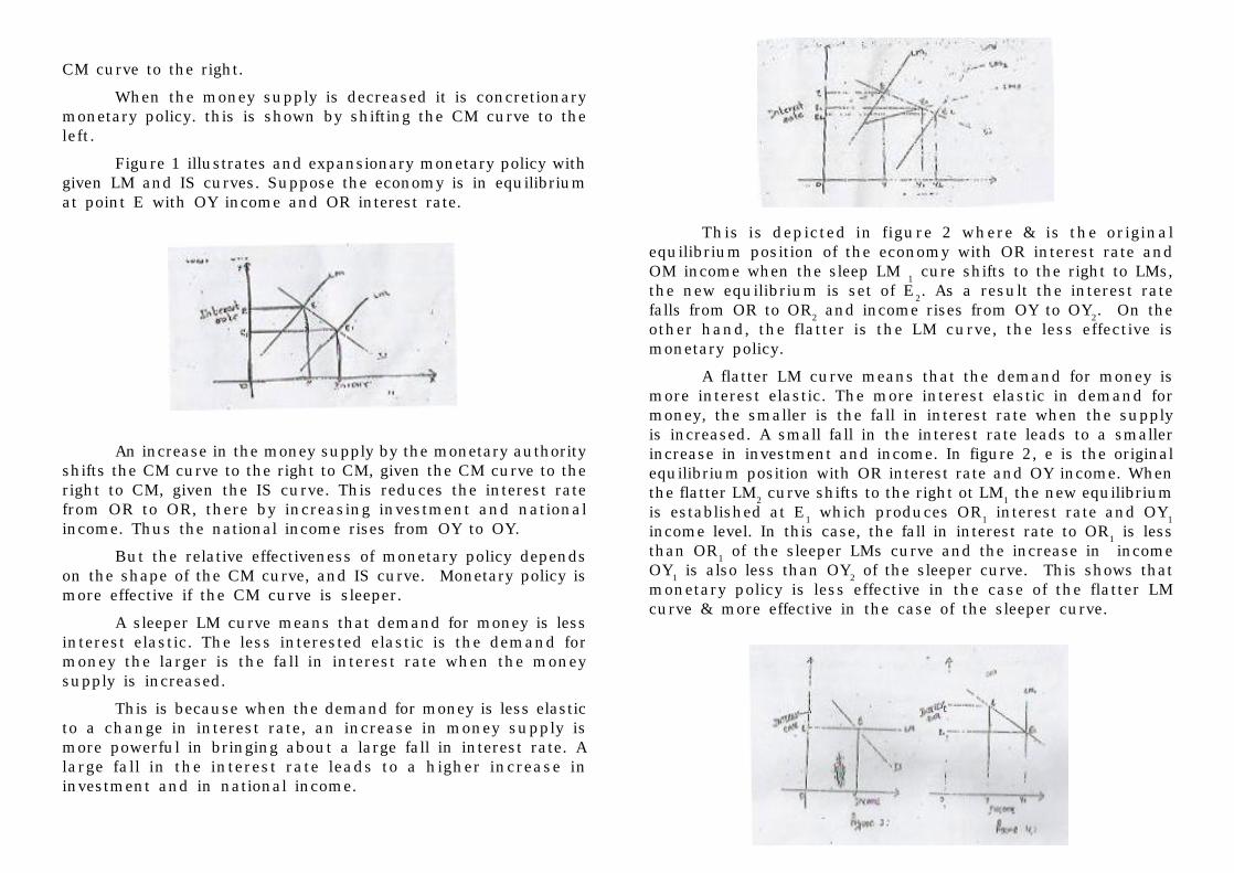
CM curve to the right.

When the money supply is decreased it is concretionarymonetary policy. this is shown by shifting the CM curve to theleft.

Figure 1 illustrates and expansionary monetary policy withgiven LM and IS curves. Suppose the economy is in equilibriumat point E with OY income and OR interest rate.

An increase in the money supply by the monetary authorityshifts the CM curve to the right to CM, given the CM curve to theright to CM, given the IS curve. This reduces the interest ratefrom OR to OR, there by increasing investment and nationalincome. Thus the national income rises from OY to OY.

But the relative effectiveness of monetary policy dependson the shape of the CM curve, and IS curve. Monetary policy ismore effective if the CM curve is sleeper.

A sleeper LM curve means that demand for money is lessinterest elastic. The less interested elastic is the demand formoney the larger is the fall in interest rate when the moneysupply is increased.

This is because when the demand for money is less elasticto a change in interest rate, an increase in money supply ismore powerful in bringing about a large fall in interest rate. Alarge fall in the interest rate leads to a higher increase ininvestment and in national income.

This is depicted in figure 2 where & is the originalequilibrium position of the economy with OR interest rate andOM income when the sleep LM 1 cure shifts to the right to LMs,the new equilibrium is set of E2. As a result the interest ratefalls from OR to OR2 and income rises from OY to OY2. On theother hand, the flatter is the LM curve, the less effective ismonetary policy.

A flatter LM curve means that the demand for money ismore interest elastic. The more interest elastic in demand formoney, the smaller is the fall in interest rate when the supplyis increased. A small fall in the interest rate leads to a smallerincrease in investment and income. In figure 2, e is the originalequilibrium position with OR interest rate and OY income. Whenthe flatter LM2 curve shifts to the right ot LM1 the new equilibriumis established at E1 which produces OR1 interest rate and OY1income level. In this case, the fall in interest rate to OR1 is lessthan OR1 of the sleeper LMs curve and the increase in incomeOY1 is also less than OY2 of the sleeper curve. This shows thatmonetary policy is less effective in the case of the flatter LMcurve & more effective in the case of the sleeper curve.

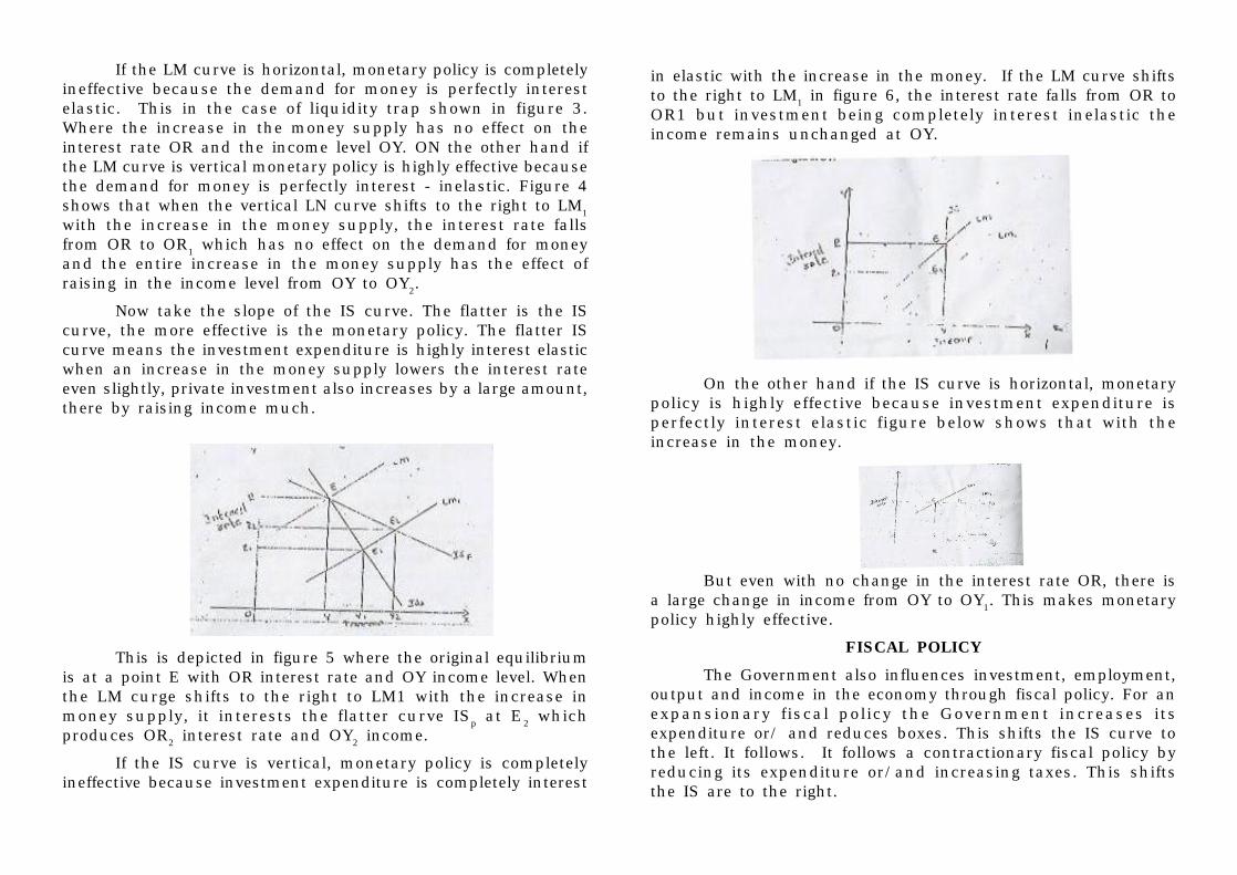
If the LM curve is horizontal, monetary policy is completelyineffective because the demand for money is perfectly interestelastic. This in the case of liquidity trap shown in figure 3.Where the increase in the money supply has no effect on theinterest rate OR and the income level OY. ON the other hand ifthe LM curve is vertical monetary policy is highly effective becausethe demand for money is perfectly interest - inelastic. Figure 4shows that when the vertical LN curve shifts to the right to LM1with the increase in the money supply, the interest rate fallsfrom OR to OR1 which has no effect on the demand for moneyand the entire increase in the money supply has the effect ofraising in the income level from OY to OY2.

Now take the slope of the IS curve. The flatter is the IScurve, the more effective is the monetary policy. The flatter IScurve means the investment expenditure is highly interest elasticwhen an increase in the money supply lowers the interest rateeven slightly, private investment also increases by a large amount,there by raising income much.

This is depicted in figure 5 where the original equilibriumis at a point E with OR interest rate and OY income level. Whenthe LM curge shifts to the right to LM1 with the increase inmoney supply, it interests the flatter curve ISp at E2 whichproduces OR2 interest rate and OY2 income.

If the IS curve is vertical, monetary policy is completelyineffective because investment expenditure is completely interest

in elastic with the increase in the money. If the LM curve shiftsto the right to LM1 in figure 6, the interest rate falls from OR toOR1 but investment being completely interest inelastic theincome remains unchanged at OY.

On the other hand if the IS curve is horizontal, monetarypolicy is highly effective because investment expenditure isperfectly interest elastic figure below shows that with theincrease in the money.

But even with no change in the interest rate OR, there isa large change in income from OY to OY1. This makes monetarypolicy highly effective.

FISCAL POLICYThe Government also influences investment, employment,

output and income in the economy through fiscal policy. For anexpansionary fiscal policy the Government increases itsexpenditure or/ and reduces boxes. This shifts the IS curve tothe left. It follows. It follows a contractionary fiscal policy byreducing its expenditure or/and increasing taxes. This shiftsthe IS are to the right.

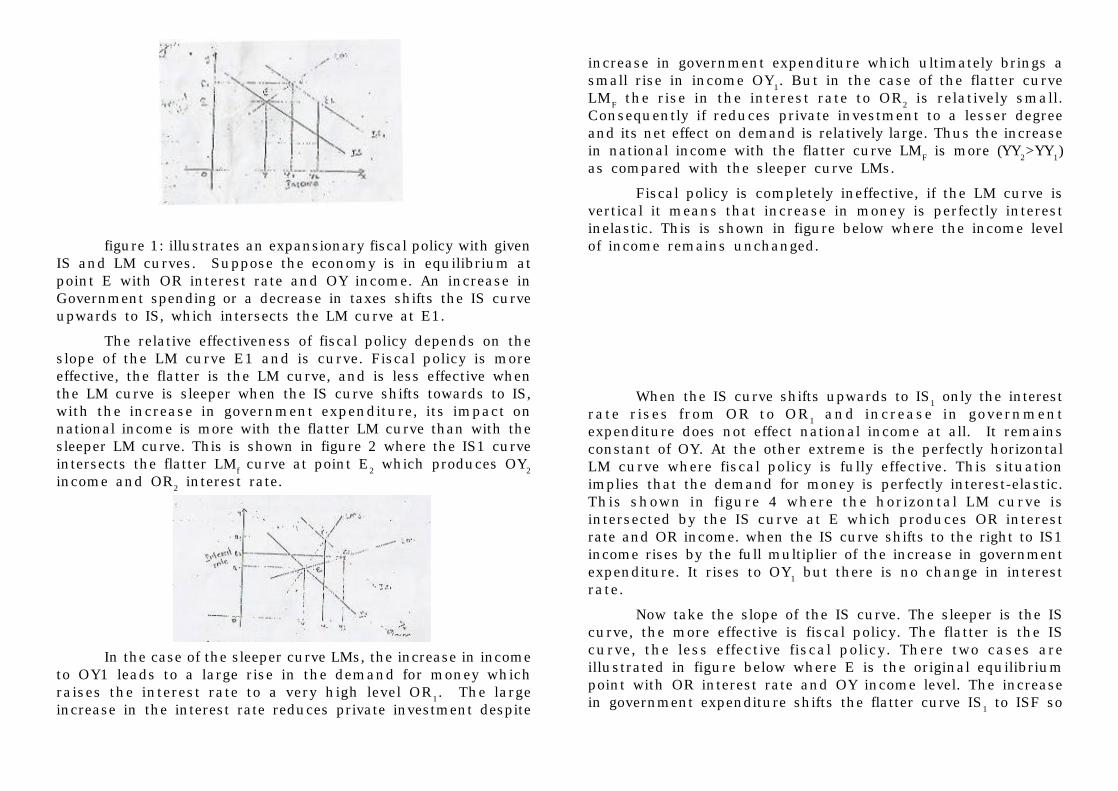
figure 1: illustrates an expansionary fiscal policy with givenIS and LM curves. Suppose the economy is in equilibrium atpoint E with OR interest rate and OY income. An increase inGovernment spending or a decrease in taxes shifts the IS curveupwards to IS, which intersects the LM curve at E1.

The relative effectiveness of fiscal policy depends on theslope of the LM curve E1 and is curve. Fiscal policy is moreeffective, the flatter is the LM curve, and is less effective whenthe LM curve is sleeper when the IS curve shifts towards to IS,with the increase in government expenditure, its impact onnational income is more with the flatter LM curve than with thesleeper LM curve. This is shown in figure 2 where the IS1 curveintersects the flatter LMf curve at point E2 which produces OY2income and OR2 interest rate.

In the case of the sleeper curve LMs, the increase in incometo OY1 leads to a large rise in the demand for money whichraises the interest rate to a very high level OR1. The largeincrease in the interest rate reduces private investment despite

increase in government expenditure which ultimately brings asmall rise in income OY1. But in the case of the flatter curveLMF the rise in the interest rate to OR2 is relatively small.Consequently if reduces private investment to a lesser degreeand its net effect on demand is relatively large. Thus the increasein national income with the flatter curve LMF is more (YY2>YY1)as compared with the sleeper curve LMs.

Fiscal policy is completely ineffective, if the LM curve isvertical it means that increase in money is perfectly interestinelastic. This is shown in figure below where the income levelof income remains unchanged.

When the IS curve shifts upwards to IS1 only the interestrate rises from OR to OR1 and increase in governmentexpenditure does not effect national income at all. It remainsconstant of OY. At the other extreme is the perfectly horizontalLM curve where fiscal policy is fully effective. This situationimplies that the demand for money is perfectly interest-elastic.This shown in figure 4 where the horizontal LM curve isintersected by the IS curve at E which produces OR interestrate and OR income. when the IS curve shifts to the right to IS1income rises by the full multiplier of the increase in governmentexpenditure. It rises to OY1 but there is no change in interestrate.

Now take the slope of the IS curve. The sleeper is the IScurve, the more effective is fiscal policy. The flatter is the IScurve, the less effective fiscal policy. There two cases areillustrated in figure below where E is the original equilibriumpoint with OR interest rate and OY income level. The increasein government expenditure shifts the flatter curve IS1 to ISF so

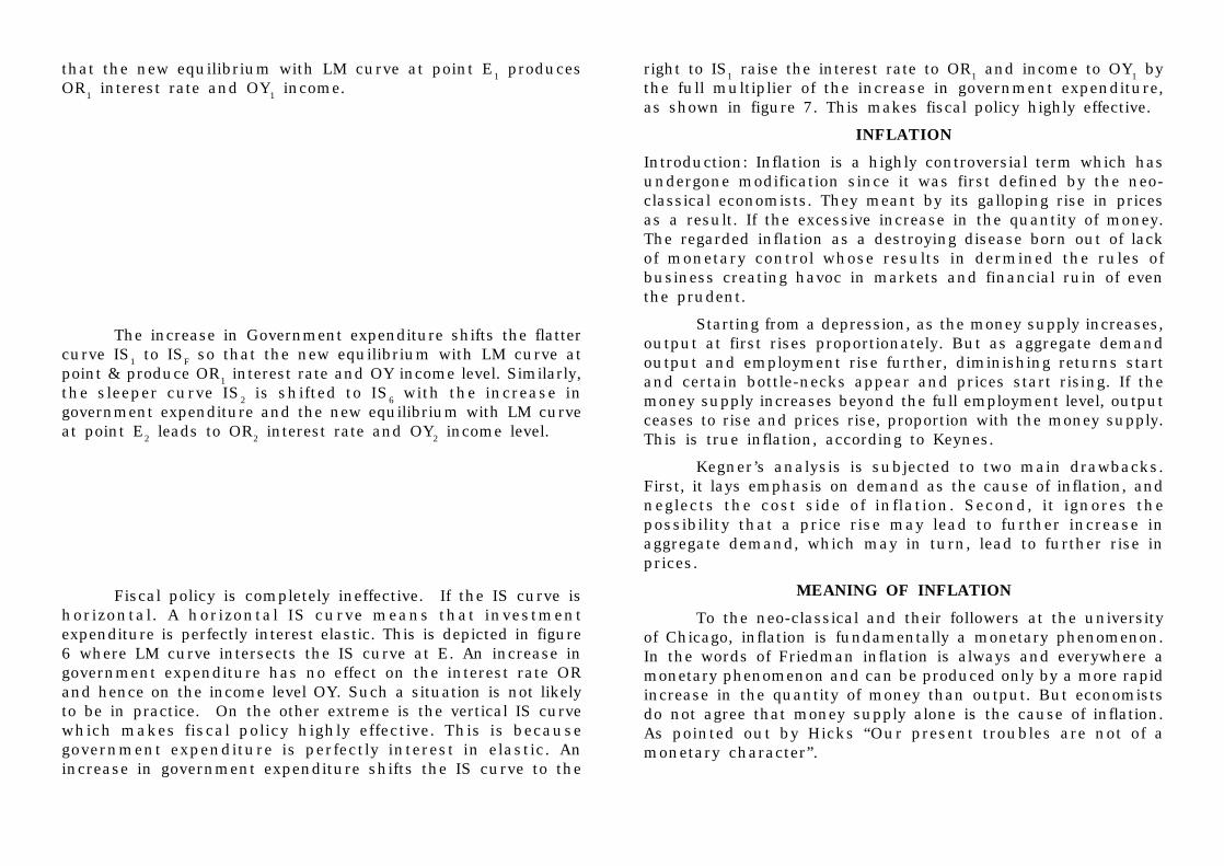
that the new equilibrium with LM curve at point E1 producesOR1 interest rate and OY1 income.

The increase in Government expenditure shifts the flattercurve IS1 to ISF so that the new equilibrium with LM curve atpoint & produce OR1 interest rate and OY income level. Similarly,the sleeper curve IS2 is shifted to IS6 with the increase ingovernment expenditure and the new equilibrium with LM curveat point E2 leads to OR2 interest rate and OY2 income level.

Fiscal policy is completely ineffective. If the IS curve ishorizontal. A horizontal IS curve means that investmentexpenditure is perfectly interest elastic. This is depicted in figure6 where LM curve intersects the IS curve at E. An increase ingovernment expenditure has no effect on the interest rate ORand hence on the income level OY. Such a situation is not likelyto be in practice. On the other extreme is the vertical IS curvewhich makes fiscal policy highly effective. This is becausegovernment expenditure is perfectly interest in elastic. Anincrease in government expenditure shifts the IS curve to the

right to IS1 raise the interest rate to OR1 and income to OY1 bythe full multiplier of the increase in government expenditure,as shown in figure 7. This makes fiscal policy highly effective.

INFLATIONIntroduction: Inflation is a highly controversial term which hasundergone modification since it was first defined by the neo-classical economists. They meant by its galloping rise in pricesas a result. If the excessive increase in the quantity of money.The regarded inflation as a destroying disease born out of lackof monetary control whose results in dermined the rules ofbusiness creating havoc in markets and financial ruin of eventhe prudent.

Starting from a depression, as the money supply increases,output at first rises proportionately. But as aggregate demandoutput and employment rise further, diminishing returns startand certain bottle-necks appear and prices start rising. If themoney supply increases beyond the full employment level, outputceases to rise and prices rise, proportion with the money supply.This is true inflation, according to Keynes.

Kegner’s analysis is subjected to two main drawbacks.First, it lays emphasis on demand as the cause of inflation, andneglects the cost side of inflation. Second, it ignores thepossibility that a price rise may lead to further increase inaggregate demand, which may in turn, lead to further rise inprices.

MEANING OF INFLATIONTo the neo-classical and their followers at the university

of Chicago, inflation is fundamentally a monetary phenomenon.In the words of Friedman inflation is always and everywhere amonetary phenomenon and can be produced only by a more rapidincrease in the quantity of money than output. But economistsdo not agree that money supply alone is the cause of inflation.As pointed out by Hicks “Our present troubles are not of amonetary character”.

However, it is essential to understand that a sustainedrise in prices may be of various magnitudes. Accordingly, differentnames have been gives to inflation depending upon the rule ofrise in prises.

1. Creeping inflation: When the rise in prices is very slow likethat of snail or creeper, it is called creeping inflation. Increaseof speed, a sustained rise in prices of annual increases of lessthan 3 percent per annum is characterized as creeping inflation.Such an increase in prices is regarded safe and essential foreconomic growth.

2. Walking or Trotting inflation: When prices rise moderatelyand the annual inflation rate is a single digit. In other words,the rate of rise in prices is in the intermediate range of 3 to 7per annum or less than 10 percent. Inflation at this rate is awarming signal for the government to control it before it turnsinto running inflation.

TRADE CYCLESIntroduction: The economic progress the world has achieved hasnot been a steady and continuous movement forward. Economicactivities faced fluctuations at more or less regular intervals.There were upward swings and downward swings. A period ofprosperity was generally followed by a period of depression. Theseups and downs in the economic activity moving like aware atregular intervals is known as business cycle (or) trade cycles.Trade cycle simply means the whole course of business activitywhich passes through the phases of prosperity and depression.

The trade cycle influence business decisions. The cycleeffects not all but each individual business firm.

The period of prosperity promotes a period business. Itprovides new investment opportunities. Likewise, a period ofdepression slackness business. A manager who is alwaysconfronted with the problem of forward planning takes intoconsideration the phases of the business cycle. This helps totake advantage of the chances a head or to reduce the chancesof heavy losses of the firm.

PHASES OF A TRADE CYCLEIntroduction: A typical cycle is generally divided into four phases.

1. Expansion or prosperity or the upswing.

2. Recession or upper - turning point.

3. Contraction or depression or downswing.

4. Revival or recovery or lower turning point.

These phases are recurrent and uniform in the case ofdifferent cycles. But no phase has definite periodicity or timeinterval. As pointed out by Pigou, cycles may not be twins butthey are of the same family. And this is shown in figure belowwhere E is the equilibrium position. We describe below thesecharacteristics of trade cycle.

1. Prosperity: In the prosperity phase, demand, output,employment, and income are at a high level. They tend to riseprices. But wages, salaries, interest rates, rentals & taxes donot rise in proportion to the rise in prices. The gap betweenprices and costs increases the margin of profit.

The gap between prices and costs increases the margin ofprofit. The increase of profit and the prospect of its continuancecommonly cause a rapid rise in stock markets. All searitiesincluding bonds, rise under the influence of improvingexpectations. The outstanding change is in stocks, that, reflectingthe capitalized values of prospective earnings, register is anexaggerated from the rising profits of enterprise.

2. Recession: Once the economy reaches the peak the coursechanges. A downward tendency in demand is observed. But the

producers who are not aware of this go on producing. The supplynow exceeds demand. Now the producers came to notice thattheir stocks are pilling up. They are compelled, to give up futureinvestment plans. The order for new equipments and rawmaterials are cancelled. A businessman even cuts down hisexisting business. Workers are retrenched. Capital goodsproducers who lose orders, in turn, cancel orders for their inputs.Bankers insist on repayment stocks accumulate.

3. Depression: Underemployment of both men & materials is acharacteristic of this phase. General demand falls faster thanproduction. Producers are compelled to sell their goods at a pricewhich will not even cover the full cost. As a consequence workersare thrown cost. The remaining workers are poorly paid. Thedemand for bank credit is at its lowest which results in idlefunds. The interest’s rate also define.

4. Recovery: Depression phase does not continue indefinitely.Depression contains in itself the germs of recovery. The idleworkers now come forward to work at low wags. As the pricesare at its lowest the consumers, who postponed their consumptionexpecting a still further fall in price, now start consuming. Thebank with accumulated cash reserves, now come forward to giveloans at easier terms and lower rates.

THEORIES AND CORRECTIVE MEASURES OF TRADECYCLES:The main theories of business cycle are

1. Monetary Theory

2. Psychological theory

3. Climatic theory

4. Innovation theory

5. Hicks theory

1. Monetary theory: Prof. R.G. Hawtrey is the main proponent ofthis theory. He views business cycle as a purely monetaryphenomenon. According to his theory the main reason for

business cycle is the unstable bank credit system. The inflationaryand deflationary factors rising from the credit facility monitoredby banks are the forces at behind the business cycles. An increasein bank credit results is an obstacle for the business cycle. Themoney borrowed is used for the payment of wages, interest, rentetc. This is turn increases demand, price and profit which againincreases production. When the bank credit is curtailed pricesdecrease, profit decrease and production falls.

This theory considers the businessmen are highlysensitive to changes in the interest rate. The businessmen aremore concerned about the future business prospects than of thechanges in the interest rate. Business cycle cannot be consideredpurely a monetary phenomenon though it is a major contributingfactor. Further this theory does not full explain the turningpoints of the business cycle.

2. Psychological theory: Prof. A.C. Pigou is considered as themain advocate of this theory. Pigou holds that there are wavesof optimism and pessimism in the human mind. When a slightprice increase is felt the human mind becomes optimistic. Theleading business firms, in expectation of a further rise in priceand profitability intensity their business. This optimism is passedto other businessman. The total economy now swings upward.this results in increase in the costs of the factors of productionwhich in turn reduces the profit margin.

3. Climatic Theory: Harvest or climatic theory is one of the oldestexplanations of business cycle. This theory relates business cycleto climatic changes. The business cycle, according to this theory,starts in the agricultural sector and spreads to industrial sector.