Real Estate Metrics: Numbers Never Lie or Do They?

What are the Important Real Estate Metrics and Why Do They Matter?

Thomas F. Kaufman

General. Real estate has been a key component of everyday life since the adaptation of mankind into an agrarian society thousands of years ago. While not as high tech as flash trading and Silicon Valley businesses, it is still data driven. Can I rent this property and for what amount? What are competing rents and sales prices? What are financing costs for this class of property? Will additional tenant improvements generate a sufficient return to make the investment worthwhile?

Metrics are imbedded into all aspects of real estate, not just at the basic property level as above, but as an overall guide as to how real estate compares to other investment classes. Most importantly, without numbers how do you measure real estate risks and rewards to see if the return is sufficient given the underlying risks?

Lawyers in general have often been thought of as weak in quantitative skills1. While recent articles have indicated that is not true2, why would a lawyer be interested in the underlying 1 Illuminating Innumeracy, Case Western Law Review Vol. 63 Spring 2013. To be clear, it says that only 13% of Americans are proficient with quantitative tasks, and that lawyers are not actually so bad in math. Many lawyers are reasonably proficient in math, but their math skills are not as developed as their verbal skills so they have a lack of confidence in their math or math anxiety. Other lawyers have just avoided math courses and have a deficit in mathematics education. The errors are characterized in this article as threefold. The first is by miscalculation such as the misapplication of discounts for lack of control and lack of marketability. Assume that the markdown for lack of control was 30% and the lack of marketability was 20%. That does not mean the markdown is 50%. Rather the discounts are applied serially:

Initial sales price $1,000,000

30% Lack of control discount -$300,000

Preliminary Sales price $700,000

20% Lack of liquidity discount -$140,000

Final Sale Price $560,000 (44% total discount)

The second source of errors is oversimplification. The third and last source of errors is misunderstanding, applying probabilities. For example in the OJ Simpson murder trial law professor Alan Dershowitz testified there was only a .04% chance that Mr. Simpson had killed his ex-wife. That was the probability that Nicole Simpson would be killed by her husband based solely upon evidence that he had battered her. The more relevant statistic, not disclosed at the trial was that the likelihood that a battered woman’s abuser was her killer once she was in fact, killed, was almost 90%.

2 Numeracy and Legal Decision Making, Arizona State Law Journal Vol. 46 pp 191-230 (2014). Lawyers, this article concludes, are not as bad at mathematics as is commonly assumed. Using the “Schwartz test” as an objective test of numeracy, they concluded that lawyers, at least those lawyers at the University of Illinois Law School had higher scores (57% answered all 3 questions accurately) than the general population (which only had 16% answer all

1

metrics? The primary reason to understand the metrics is that it helps a lawyer to better comprehend the client’s goals for a project. It also helps define what is important in the legal context because if it is important to the economics of the client’s activity, then it should be protected in the related legal documents.

A more basic reason to use and review metrics is to understand risk and its rewards in connection with any investment. Without numbers there are no odds, no probabilities and no measures and the only way to assess risk is to trust in the “Gods and fate.”3 While seat of the pants intuition is often very helpful, more detailed modeling of risk and returns is more insightful. Nevertheless, two things should be recalled. First, the best spreadsheet does not yield the best investment decision, otherwise creativity and business acumen would give way purely to spreadsheet sophistication. Second, no spreadsheet is ever 100% accurate. They are based on projections for things such as income and expenses and while they may be close in the aggregate returns sometimes, they are virtually always wrong on the minute details of the projections.

1. The Basics .

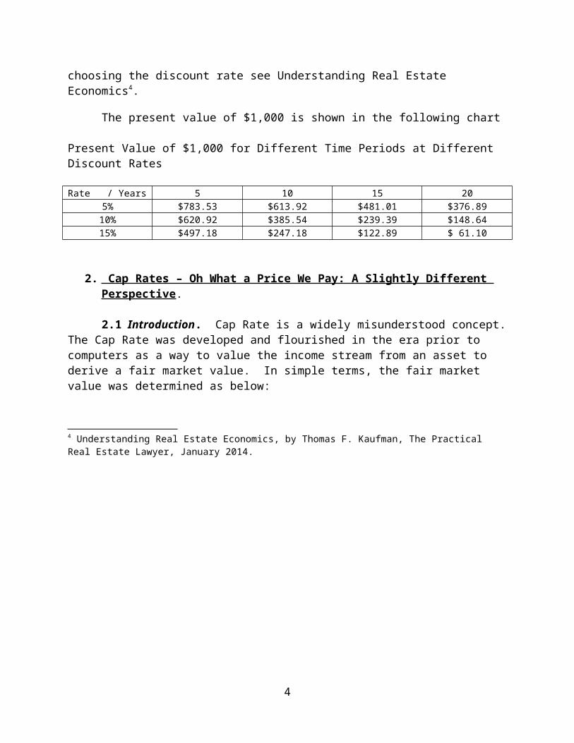
Present Value. The most fundamental concept in modeling is present value. The idea that a dollar today is worth more than a dollar in the future is the basis for determining present value. In most investments the steam of income will continue for many years from the initial investment to the ultimate sale. If a dollar today can be invested at 5 percent per annum, it will be worth approximately $1.63 in ten years. If the interest is compounded monthly then the same 5 percent per annum will yield approximately $1.65 in 10 years. To determine the correct discount factor to apply one must be able to calculate the percentage return an investor would require in order to accept the delay in the payment. That judgment is based upon (i) the nominal interest rate for a similar time period, (ii) the perceived inflation rate, (iii) the risk that the payments will not be made as required, and (iv) the simple supply and demand for money. As these figures vary constantly, the discount rate should also vary, but most times it is chosen as a constant over the entire period. For a more detailed look at present value and choosing the discount rate see Understanding Real Estate Economics4.

3 questions accurately). This could be due to the higher level of education of the Illinois law students or that they were younger than the population in general, or for numerous other reasons. The Schwartz test is simple and has only 3 questions:

1. Imagine that we flip a fair coin 1,000 times. What is your best guess as to how many times the coin would come up heads in 1,000 flips? (500) 2. In the Big Bucks Lottery, the chance of winning a $10 prize is 1%, what is your best guess about how many people would win a $10 prize if 1,000 people each buy a single ticket to Big Bucks? (10). 3. In Acme Publishing Sweepstakes, the chance of winning a car is 1 in 1,000. What percent of tickets to Acme Publishing Sweepstakes win a car? (0.1%)

57.2% of the students got all three right, 29.6% missed just one question, 10.5% gave only one correct answer and 2.6% failed to answer any question correctly.

3 Against the Gods: The Remarkable Story of Risk, Bernstein.4 Understanding Real Estate Economics, by Thomas F. Kaufman, The Practical Real Estate Lawyer, January 2014.

2

The present value of $1,000 is shown in the following chart

Present Value of $1,000 for Different Time Periods at Different Discount Rates

Rate / Years 5 10 15 205% $783.53 $613.92 $481.01 $376.8910% $620.92 $385.54 $239.39 $148.6415% $497.18 $247.18 $122.89 $ 61.10

2. Cap Rates – Oh What a Price We Pay: A Slightly Different Perspective .

2.1 Introduction. Cap Rate is a widely misunderstood concept. The Cap Rate was developed and flourished in the era prior to computers as a way to value the income stream from an asset to derive a fair market value. In simple terms, the fair market value was determined as below:

Fair Market Value = Stabilized Net Operating Income / Cap Rate

In this equation, the Stabilized Net Operating Income is the best estimate for the net operating income (“NOI”) after whatever rehabilitation, re-tenanting or project stabilization was completed. The Cap Rate is the minimum rate of return that the investor demanded from this specific investment considering the entire investment, including the risk profile of the investment. Cap Rate then becomes a determinant of what price the market will pay for an asset.

Cap Rate = Stabilized Net Operating Income / Fair Market Value

So if a property has $1,000,000 stabilized NOI and the Cap Rate is 5% then the investor would pay $20,000,000 for the asset ($1,000,000 / .05). This calculation has the virtue of simplicity even if based upon limited due diligence and all diligence going into determining the stabilized NOI. Obviously income and expenses change over time in complex manners, so this simplistic approach is not very insightful in these days of powerful computers and computer models.

The continuing appeal of Cap Rate is that it is a shorthand way to specify the level of pricing and expected returns for investors. In today’s world where the average smart phone is more powerful than a main frame computer in the early days, there are many methods of determining the price

3

for an asset. The most widely used is the Discounted Cash Flow model, which will be discussed in more detail later. Not only that, but most purchasers consider at least 5 to 20 metrics in determining rates of return and proposed pricing.5

2.2 Market Shifts. Cap Rate is also useful for determining what happens when markets shift and pricing changes accordingly. For example, in the early 2000s the pricing for many major hotels was based upon a Cap Rate in the 10-11 percent range. Today that Cap Rate is about 4.5 to 6 percent for major hotels in major gateway cities. A rise in the Cap Rate can be driven by many items. Most importantly is the perceived inflation and overall interest rates. As interest rates rise, so must Cap Rates. No one would invest in the equity of an investment if the return were less than that of debt. The rate of return on an equity capital investment must be perceived as greater than that of debt on the same asset in order to make up for the increased risk of equity ownership. That is a basic law of finance. Thus there are times when the change in Cap Rate is driven by an increase or decrease in interest rates.

The past several years have seen unusually low rates of interest with 10-year US Treasury securities in early 2015 dipping below 2% per annum. That is below their long term norm. What happens as interest rates and Cap Rates increase? As Cap Rates rise, then under the formula above, the fair market value will decrease unless the NOI is increased. It is instructive to look at how much the NOI must increase based upon Cap Rate increases to maintain pricing stability.

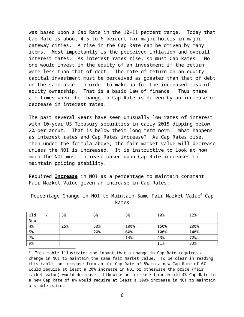
Required Increase in NOI as a percentage to maintain constant Fair Market Value given an increase in Cap Rates:

Percentage Change in NOI to Maintain Same Fair Market Value6 Cap Rates

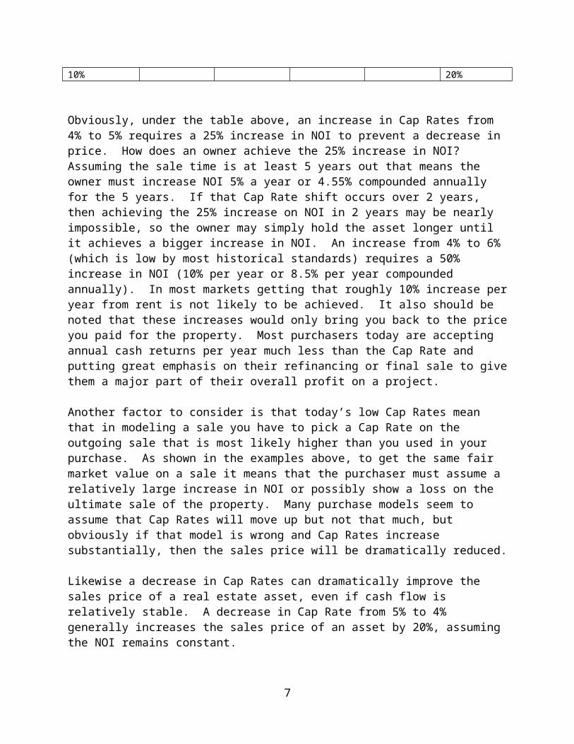
Old / New 5% 6% 8% 10% 12%4% 25% 50% 100% 150% 200%5% 20% 60% 100% 140%7% 14% 43% 72%9% 11% 33%10% 20%

Obviously, under the table above, an increase in Cap Rates from 4% to 5% requires a 25% increase in NOI to prevent a decrease in price. How does an owner achieve the 25% increase in NOI? Assuming the sale time is at least 5 years out that means the owner must increase NOI 5% a year or 4.55% compounded annually for the 5 years. If that Cap Rate shift occurs over 2 years, then achieving the 25% increase on NOI in 2 years may be nearly impossible, so the owner may simply hold the asset longer until it achieves a bigger increase in NOI. An increase from 4% to 5 See Understanding Real Estate Economics at pp 38-49.

6 This table illustrates the impact that a change in Cap Rate requires a change in NOI to maintain the same fair market value. To be clear in reading this table, an increase from an old Cap Rate of 5% to a new Cap Rate of 6% would require at least a 20% increase in NOI or otherwise the price (fair market value) would decrease. Likewise an increase from an old 4% Cap Rate to a new Cap Rate of 8% would require at least a 100% increase in NOI to maintain a stable price.

4

6% (which is low by most historical standards) requires a 50% increase in NOI (10% per year or 8.5% per year compounded annually). In most markets getting that roughly 10% increase per year from rent is not likely to be achieved. It also should be noted that these increases would only bring you back to the price you paid for the property. Most purchasers today are accepting annual cash returns per year much less than the Cap Rate and putting great emphasis on their refinancing or final sale to give them a major part of their overall profit on a project.

Another factor to consider is that today’s low Cap Rates mean that in modeling a sale you have to pick a Cap Rate on the outgoing sale that is most likely higher than you used in your purchase. As shown in the examples above, to get the same fair market value on a sale it means that the purchaser must assume a relatively large increase in NOI or possibly show a loss on the ultimate sale of the property. Many purchase models seem to assume that Cap Rates will move up but not that much, but obviously if that model is wrong and Cap Rates increase substantially, then the sales price will be dramatically reduced.

Likewise a decrease in Cap Rates can dramatically improve the sales price of a real estate asset, even if cash flow is relatively stable. A decrease in Cap Rate from 5% to 4% generally increases the sales price of an asset by 20%, assuming the NOI remains constant.

In summary, the history of interest rates and Cap Rates has been volatile, and that is expected to continue.7 With interest rates at very low levels, it is expected that interest rates will increase in the future and Cap Rates will rise with them.8 The change in Cap Rates will echo in pricing and buyers in 2015 have to take that into account in planning refinancings and final sales.

2.3 Holding Period. There is a corollary that is especially important with low Cap Rates that are expected to increase -- that if you hold the property for a very, very long time, then the ultimate sales price on the Discounted Cash Flow model will not be as significant as it is for the buyer who intends to sell the property within 5 years. In that case, the Cap Rate at the time of the distant sale will not be as large a factor. For example, if you are selling an asset in year 5 for $10,000,000 and the discount rate is say, 12% per annum, then the discounted cash flow (present value) for a sale after 5 years is $5,674,269, whereas if the asset was sold after 25 years, then the discounted cash flow (present value) of that sale is $588,233, only about 10% of the magnitude of the sale price after 5 years. Now obviously the sale price should increase over the 20 years from year 5 to year 25, but even if the value of the asset increases 3% per year, the discounted cash flow (present value) of that increased price ($18,061,112 in year 25) is still only $1,062,414. This is very small compared to the impact on the discounted cash flow of a sale in year 5.

Conversely, in times of decreasing Cap Rates and therefore increasing prices, a shorter holding period may allow an assumption in the underlying models that on the sale date the Cap Rate will decrease even more and thus the shorter term hold would be benefitted.

For example, assume one bidder is looking to hold a real estate asset for 3 years and another bidder for 10 years and the asset is worth roughly $14,285,000 and has a roughly $1,000,000

7 Moody’s 2015 Outlook – US CMBS, December 9, 2014 (“Moody’s Outlook”).8 Moody’s Outlook at pp 9-10.

5

NOI. Assume that the Cap Rate at the time of the bidding is 7%, but is trending lower because of low inflation, an improving economy and high demand for real estate. Also assume a 12% discount rate for the discounted cash flow. Maybe the bidder with the 3-year hold can project a Cap Rate of 6%, whereas the longer term hold cannot justify saying there will be any change in the Cap Rate. Then assuming a sale at the end of 3 years at a price of $15,600,000 (a 3% per year increase), the present value of the sales proceeds would be $11,103,771, whereas for a sale after 10 years, the present value of the sales proceeds would be $5,215,322 ($16,198,000 (which is the acquisition price $14,285,000 growing at 3% per year) / 3.106 (the discount factor after 10 years at a discount rate of 12%))

2.4 Moody’s Cap Rate Adjustments In its October 29, 2014 Special Comment, Moody’s Investor Service stated that “Conduit Loan Credit Quality Slippage is Déjà vu All Over Again.”9 It is an excellent analysis of the CMBS market, and it concludes that the Moody’s loan to value ratio (“MLTV”) for CMBS collateral for the 3rd Quarter of 2014 is not the 67.8% that the underwriters show, but that it is really 112.2 %10. In simple terms how can you arrive at that conclusion? One simple way is to assume that the NOI is accurate, but that the underwriter is using an aggressive Cap Rate to justify higher property values.

Let’s use an example. Assume the underwritten stabilized NOI for a property to be financed is $1,000,000 per year and use the Cap Rate cited by Moody’s as the underwritten Cap Rate of 6.37% used on this property. Then using our formula for the fair market value and Cap Rate

Fair Market Value = stabilized NOI / Cap Rate

$15,698,587 = $1,000,000 / .0637

The underwritten fair market value is then roughly $15,698,587. If the loan to value ratio is approximately 67.8% then using the formula for the LTV

LTV = Loan Amount / Fair Market Value

Loan Amount = Fair Market Value * LTV

Assuming the LTV = 67.8% then the Loan Amount would be approximately $10,643,641

$10,643,641 = $15,698,587 * 67.8%

But the Moody’s cap rate would be roughly 350 basis points higher11, or approximately 9.87%, so it would calculate a different fair market value and different LTV using the exact same stabilized NOI. Let’s look at the Moody’s calculations:

Fair Market Value = stabilized NOI / Cap Rate

9 Moody’s Special Comment , US CMBS Q3 Review: Conduit Loan Credit Quality Slippage is Déjà Vu All Over Again, October 29, 2014. (“Moody’s Special Comment”)10 Moody’s Special Comment, at page 111 See Exhibit A to this article.

6

$10, 131,712 = $1,000,000 / .0987

So the Moody’s LTV using the Moody’s Cap Rate and Moody’s Fair Market Value, but the underwritten loan amount of $10,643,641 would be:

Moody’s LTV = Actual Underwritten Loan Amount / Moody’s Fair Market Value

105% = $10,643,641 / 10,131,712

So the Moody’s LTV would be 105%, whereas the underwritten LTV was stated to be 67.8%. Obviously the Moody’s LTV of 105% is still less than the average Moody’s LTV for the 3rd Quarter of 2014, 112.2%, but that difference can be attributed to adjustments in underwritten NOI or other factors. The important thing to note is that the announced underwritten LTV is a relatively conservative 67.8%, whereas Moody’s thinks the underwriting is far too aggressive and the real Moody’s LTV is over 100% of the fair market value. Most of that difference can be accounted for by Moody’s implied restatement of the Cap Rates to take into account Moody’s belief that the aggressive pricing in the real estate market and resulting low Cap Rates are not true long term indicators of value and need to be adjusted to properly assess the finance risk.

Most importantly, Moody’s believes that there are inherent risks to the entire CMBS market if the aggressive underwriting for CMBS loans continues. “As CMBS ‘umpires’ we are prepared to call credit quality as we see it …. If the conduit loan underwriting slippage continues on its current path, it is less likely that CMBS will become a dependable source of capital over the long run and more likely that it will become a boom-and-bust business that makes real estate even more volatile.”12

2.5 Take Aways. So let’s summarize the impacts of changes in Cap Rates. The take aways with respect to Cap Rate are:

(1) That Cap Rates are still widely discussed, even though purchasers of real estate have moved on to far more complex computer based models such as discounted cash flow and use many different tests to ultimately decide to acquire a real estate asset and how much they are willing to pay for it.

(2) That in a volatile Cap Rate market, the change in Cap Rate may dramatically change the sale price of an asset to such a degree that it swamps any increase or decrease in NOI from the property.

(3) That an increase in Cap Rates requires an increase in NOI or the fair market value of the asset decreases.

(4) A decrease in Cap Rates may provide a strong return on an asset even if the NOI is relatively stable.

(5) A change in Cap Rates can create a competitive advantage for an investor with different projected holding periods for the asset. In increasing Cap Rate periods a much, much longer holding period may be an advantage. Whereas in a decreasing Cap Rate period a

12 It then quotes Yogi Berra to say that “it ain’t over til its over” and that CMBS quality could rally before it is “game over” for CMBS issuance.

7

shorter term investment horizon or property holding period may allow a potential buyer to pay more for an asset than a longer term investor. In both of these cases this assumes that the NOI would be relatively the same for each investor.

(6) Aggressive Cap Rates may not be long term indicators of value and underwriters and rating agencies may adjust for very low Cap Rates.

3. Computer Modeling

3.1 Introduction Today the ubiquitous computer and spreadsheet have changed real estate modeling dramatically. They allow sophisticated models and major variations to be run and tested easily. Market data is readily obtainable and models can be revised to the point of almost driving the user to indecision because so many variations are possible. There is one axiom to remember however – the best model does not engender finding the best purchase price or the best long term outcome. He who has the best model does not have the best real estate business. Most often cleverness, execution and a bit of luck make more difference than the best models.

Compared to simple present value calculations and Cap Rates, multi-period computer models make analysis of rates of return much more sophisticated and better able to track and project future outcomes and provide better data for decision making. Real estate models are projections based upon estimates of future events and, like all projections, are subject to uncertainties. Only in hindsight can the actual performance of an asset be judged with certainty. Among the difficulties that affect models are the following.

3.2 Unforeseeable Events

. Sometimes projections are wrong because events occur that are truly unforeseeable. Hotel performance suffered after September 11, 2001 in a way that no one could have predicted when the U.S. travel and tourism industry went into a long and unexpected downturn because of the attacks. Sometimes the unforeseeability is debatable. Long-term Capital Management went into a financial meltdown in 1998 as a result of highly unusual events after the collapse of the Russian bond market.13 Two Nobel laureates and the legendary trader John Meriwether were key figures in Long-term Capital Management, but they did not see the debacle in their models before it arrived. Upon further review, some analysts say more stress testing could have predicted the problem and more liquidity would have allowed the company to wait out the crisis.14 Other authors believe that most investors do not adequately account for the part that randomness plays in investments and that these risks of major changes are not adequately built into the pricing of investments.15 Another way to deal with these unknown risks is to greatly

13 The flight to liquidity and away from the portfolios of Russian and other illiquid bonds were outside the margins of likely behavior used in the models. Roger Lowenstein, When Genius Failed: The Rise and Fall of Long-Term Capital Management (Random House 2000) (“LTCM”). See also, Nicholas Dunbar, Inventing Money: The Story of Long-Term Capital Management and the Legends Behind It (Wiley 2000).

14 LTCM, supra.15 Nassim Nicholas Taleb, Fooled by Randomness: The Hidden Role of Chance in Life and in the Markets (Random

House, 2d ed. 2005).

8

increase liquidity and capital reserves to be able to wait out these often temporary market distortions.16

3.3 Unrealistic Sale Prices

. Many modeling problems can be self-induced. In a red-hot market with high real estate prices, analysts are tempted to push the models to justify ever higher acquisition prices. Since real estate rents are generally slower to react in such a market, the obvious pressure is to assume continued increases in the sale price of the project. Today in most cases, the success of the acquisition often turns on the sale price obtained at the end because rents and, therefore, cash flow during the holding period have not escalated as quickly as the property values. In the present era of historically low cap rates resulting in high real estate prices, using ending cap rates many years out that are still low by historic standards to calculate the final sale price is hard to justify. Many analysts often increase the cap rate on the final sale by .5 percent to 1 percent and think that is conservative, but if the initial price was based upon a discount rate or IRR that was at a 20-year low, wouldn’t it be prudent to assume that upon a final sale that discount rate or IRR had returned to more normal historic levels?

3.4 Income and Expense Growth

. Many models have a difficult time modeling the growth rates for income and expense items. The use of rent stops and pass-through of most utility and other operating expenses have removed the risk from landlords of the past problems where rapidly escalating utilities with no ability to pass increases to the tenant turned good investments into bankruptcies. Nevertheless many models project increasing operating efficiencies that will be achieved, but don’t create a contingency adequate to cover problems that they didn’t anticipate. Studies have shown that older buildings have an increasing ratio of expense to income, and these studies and the costs of aging are often ignored in the modeling.

3.5 Projected Rent Increases and Lease-Up

. Often rent renewal rates or future lease rents are based upon optimistic assumptions that will not be fulfilled. Very few models also show any flat periods of rent growth after maybe the first year or two, even in markets that have historic rent drops and cyclical leasing problems. Models must take into account the local market and its historic cycles. The same is true for the period of lease-up. It often takes much longer than expected to get a new tenant into a space and paying rent. Also the costs of replacing a single large tenant with multiple tenants, both in terms of time and tenant improvements, is often greater than modeled. A corollary is that many purchasers over-estimate the likelihood that an existing tenant will renew the lease upon expiration. This also produces unrealistic models for tenant turn-over costs.

3.6 Vacancy and Collection Losses

16 In Long-term Capital Management, if they had the capital and liquidity, the investors could have waited out the market and extracted themselves with a profit. Instead, many of them lost all their investment and several, including John Meriwether, had huge personal financial losses. See LTCM.

9

. Vacancy rates vary widely over time, yet most models show a fixed percentage for vacancy loses over the entire time of ownership after some re-leasing period. Local models are usually available to better predict these vacancies. Are vacancies shown as 5 - 7.5 percent after stabilization reasonable, when historic vacancies in the locality are often in double digits? Clearly a property that is entirely net leased to a credit tenant does not have to deal with vacancy, but most rent rolls have to model it.

3.7 Failing to Model Events after the Projected Holding Period

. An ancillary problem to that of unjustifiably increased exit sale price discussed in Section 5.2 is that many models use a simplistic cap rate model to project the sales prices. Typically sales prices are established by capitalizing the last year of net operating income. In many cases that is fine since the property is already at a stabilized income, but in a large number of properties there is additional information available. Some models do not always take into account known rental information that extends beyond the projected sales date. The more property-specific information used in modeling the sales price, the more reliable the price. For example, if some of the leases run for 15 years, then a specific model of actual rents over for that extended period provides a more accurate reversion sales price. Another possibility is to use Monte Carlo modeling17 to generate some additional feel for and sensitivity to the likely range of sale values.

4. More Complex Analysis – Payback, NPVs, IRRs and Limited Resources

4.1 Payback

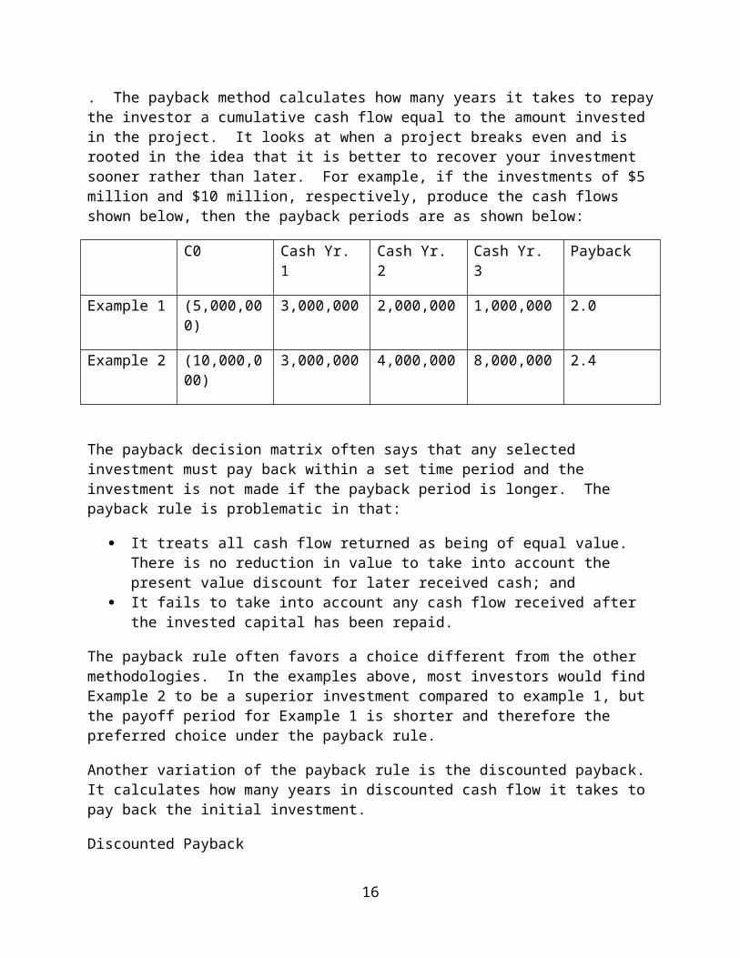
. The payback method calculates how many years it takes to repay the investor a cumulative cash flow equal to the amount invested in the project. It looks at when a project breaks even and is rooted in the idea that it is better to recover your investment sooner rather than later. For example, if the investments of $5 million and $10 million, respectively, produce the cash flows shown below, then the payback periods are as shown below:

C0 Cash Yr. 1 Cash Yr. 2 Cash Yr. 3 Payback

Example 1 (5,000,000) 3,000,000 2,000,000 1,000,000 2.0

Example 2 (10,000,000) 3,000,000 4,000,000 8,000,000 2.4

The payback decision matrix often says that any selected investment must pay back within a set time period and the investment is not made if the payback period is longer. The payback rule is problematic in that:

It treats all cash flow returned as being of equal value. There is no reduction in value to take into account the present value discount for later received cash; and

17 Monte Carlo modeling is beyond the scope of this article, but See Understanding Real Estate Economics at pp 46-47.

10

It fails to take into account any cash flow received after the invested capital has been repaid.

The payback rule often favors a choice different from the other methodologies. In the examples above, most investors would find Example 2 to be a superior investment compared to example 1, but the payoff period for Example 1 is shorter and therefore the preferred choice under the payback rule.

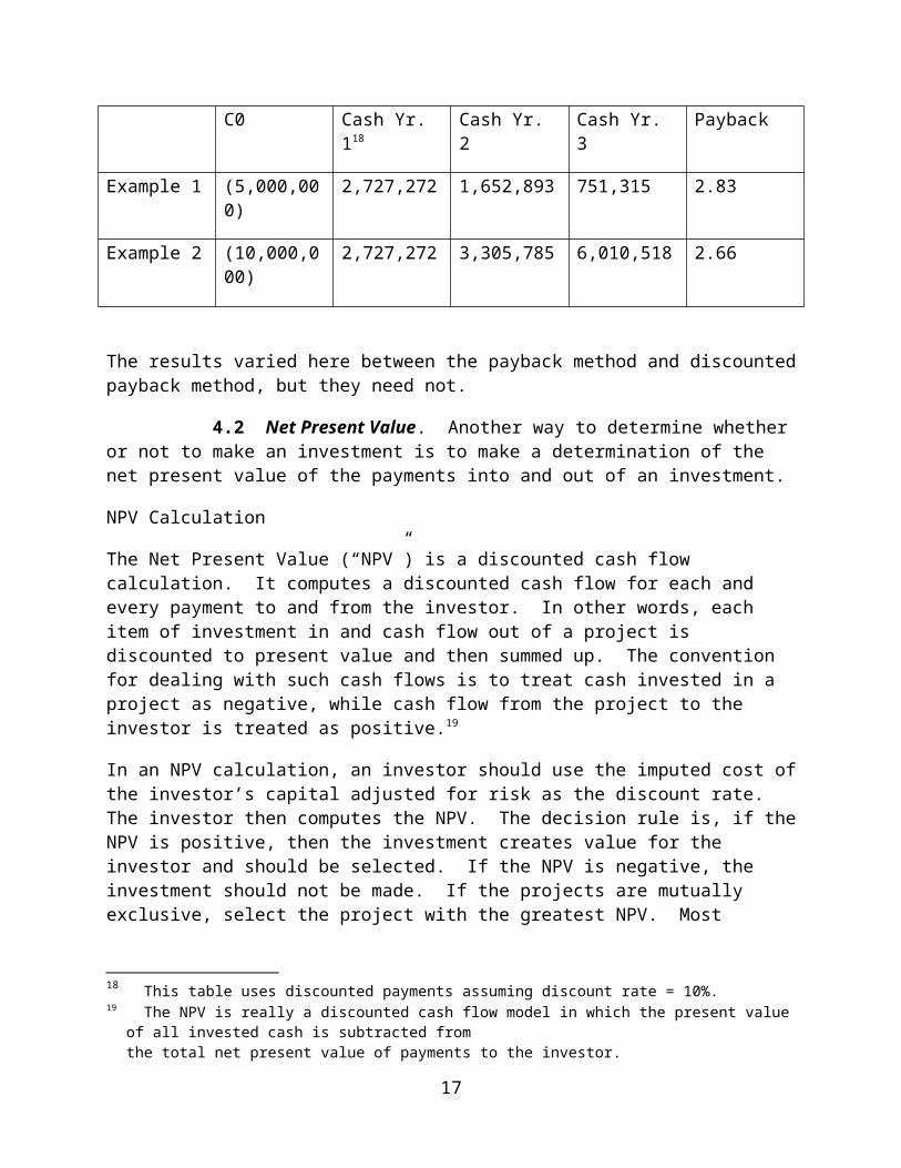
Another variation of the payback rule is the discounted payback. It calculates how many years in discounted cash flow it takes to pay back the initial investment.

Discounted PaybackC0 Cash Yr. 118 Cash Yr. 2 Cash Yr. 3 Payback

Example 1 (5,000,000) 2,727,272 1,652,893 751,315 2.83

Example 2 (10,000,000) 2,727,272 3,305,785 6,010,518 2.66

The results varied here between the payback method and discounted payback method, but they need not.

4.2 Net Present Value. Another way to determine whether or not to make an investment is to make a determination of the net present value of the payments into and out of an investment.

NPV Calculation

The Net Present Value (“NPV”) is a discounted cash flow calculation. It computes a discounted cash flow for each and every payment to and from the investor. In other words, each item of investment in and cash flow out of a project is discounted to present value and then summed up. The convention for dealing with such cash flows is to treat cash invested in a project as negative, while cash flow from the project to the investor is treated as positive.19

In an NPV calculation, an investor should use the imputed cost of the investor’s capital adjusted for risk as the discount rate. The investor then computes the NPV. The decision rule is, if the NPV is positive, then the investment creates value for the investor and should be selected. If the NPV is negative, the investment should not be made. If the projects are mutually exclusive, select the project with the greatest NPV. Most academics20 argue that this is inherently the best system because it allows a better allocation of resources when resources are constrained. In other words, if a developer cannot undertake all projects because of limited resources, the NPV

18 This table uses discounted payments assuming discount rate = 10%.19 The NPV is really a discounted cash flow model in which the present value of all invested cash is subtracted

from the total net present value of payments to the investor.

20 See Richard A. Brealey, Stewart C. Myers, and Franklin Allen, Principles of Corporate Finance (McGraw Hill/Irwin 11th ed. 2013).

11

method allows a better allocation to maximize the benefits of capital budgeting given the limitations. Examples below will show how this and other methods can be used to determine the best investments when resources are limited. The benefits of using NPV are:

The method recognizes that cash today is worth more than tomorrow; Complex models of pricing for the ultimate sale of the property are options; Since all amounts are discounted to today’s dollars, they can be added and subtracted; Complex modeling of rent streams and lease terminations fundamentally reflect the

known rent roll for a property; The model permits estimates of future rentals as vacancies appear; Capital expenditures common for most real estate projects are extensively modeled; The method of accounting does not affect the value; and The model allows an investor to more easily determine the costs and benefits of increases

or decreases in the time to complete or lease-up the project.

Problems with using an NPV calculation are:

The discount rate is generally fixed for the entire period21 while the comparable spot discount rates vary over time;

In complex examples of limited resources with multiple projects, linear programming is needed to determine the optimum investment; and

The NPV calculation effectively assumes that monies received during the term of the investment earn an amount equal to the discount rate, which is usually set based upon the investor’s cost of funds. In most short-term environments this investment rate cannot be obtained. That is especially true in the environment when this article is being written. The 10 year US Treasury bond is yielding about 2.2% and the six month US Treasury security yields about .10% per annum. None of them are close to matching the expected returns from real estate investments. An alternate methodology is to use a modified IRR also known as an MIRR. In determining a MIRR the reinvestment rate is not presumed to be the same as the underlying investment, but some other specified rate, possibly such as a 6 month US Treasury security. Obviously that could make the MIRR lower than the IRR especially for projects where a lot of the returns are generated early in the investment and the alternate investment rate is dramatically lower than the return on the underlying investment.

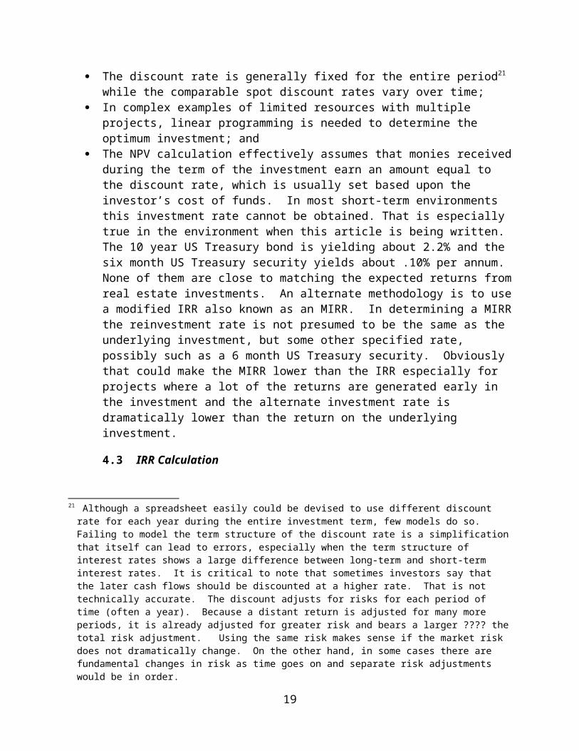
4.3 IRR Calculation

. The IRR method is a variation of the NPV which calculates the discounted cash flow of each and every payment into and out of the project. In fact, the IRR is a specific solution where the

21 Although a spreadsheet easily could be devised to use different discount rate for each year during the entire investment term, few models do so. Failing to model the term structure of the discount rate is a simplification that itself can lead to errors, especially when the term structure of interest rates shows a large difference between long-term and short-term interest rates. It is critical to note that sometimes investors say that the later cash flows should be discounted at a higher rate. That is not technically accurate. The discount adjusts for risks for each period of time (often a year). Because a distant return is adjusted for many more periods, it is already adjusted for greater risk and bears a larger ???? the total risk adjustment. Using the same risk makes sense if the market risk does not dramatically change. On the other hand, in some cases there are fundamental changes in risk as time goes on and separate risk adjustments would be in order.

12

NPV is equal to zero. In other words the IRR method iteratively calculates the discount rate that leads to an NPV of zero and this becomes the IRR. The major attraction of the IRR is that it reduces to a single number the return on a real estate investment. If the imputed cost of capital to the investor is less than the IRR, then the decision should be to invest in the project. If the imputed cost of capital is greater than the IRR, then the investment should be passed over. For example, if the imputed cost of capital for a REIT is 7 percent, then accepting a property with an IRR of 10 percent creates value for the REIT, but a property with a projected IRR of 6 percent should not be selected as it destroys value.

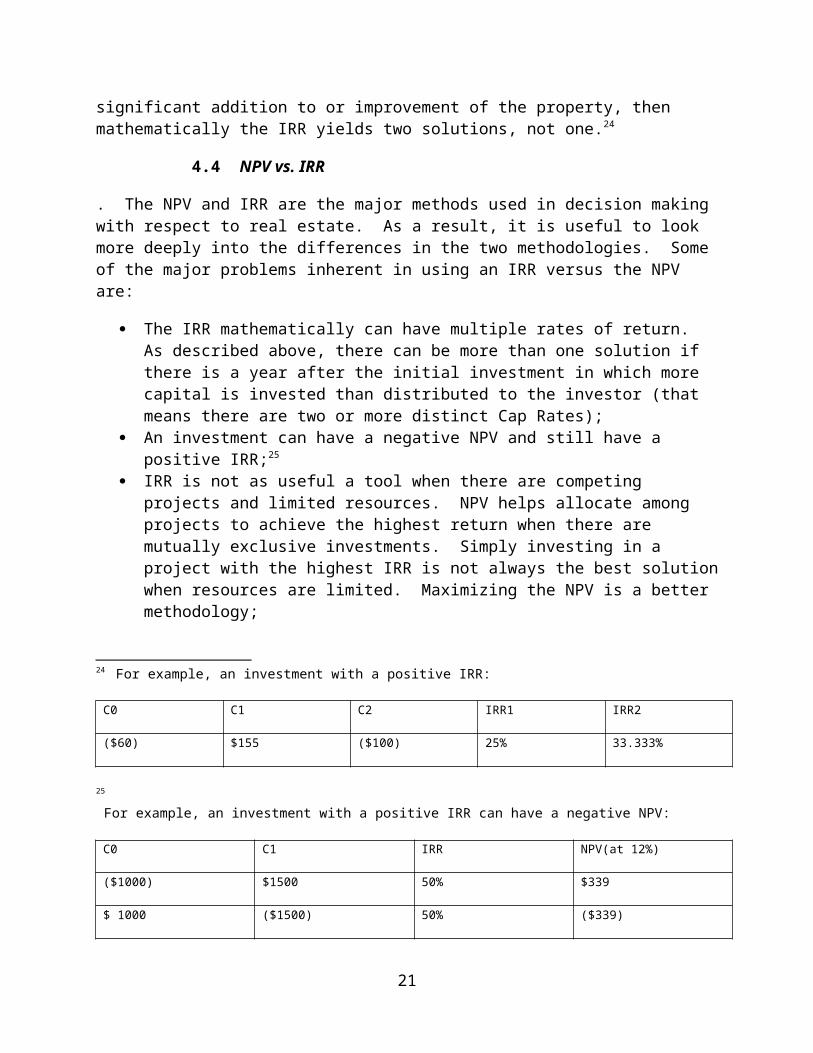
An IRR calculation assumes that all payments from and additions to the project earn the same rate of return. In reality the IRR assumption on earnings on cash distributed to the investor often results in earnings assumptions that cannot be met. For example, if an investor is able to get a 20 percent IRR, the model assumes that the investor can invest all payments received during the investment period at the same 20 percent.22 In a short-term interest rate environment of 3 percent, it introduces a distortion to assume that all payments receive the same 20 percent yield. One of the ways to remedy that is to set a re-investment rate that is realistic, given short-term rates, and compute a modified IRR. Another issue with an IRR calculation is that mathematically every time there is a year where contributions to the project exceeds the return for that year there is an additional solution to the IRR.23 In other words, if there is a major capital investment in year 2, maybe to pay for a significant addition to or improvement of the property, then mathematically the IRR yields two solutions, not one.24

4.4 NPV vs. IRR

. The NPV and IRR are the major methods used in decision making with respect to real estate. As a result, it is useful to look more deeply into the differences in the two methodologies. Some of the major problems inherent in using an IRR versus the NPV are:

The IRR mathematically can have multiple rates of return. As described above, there can be more than one solution if there is a year after the initial investment in which more capital is invested than distributed to the investor (that means there are two or more distinct Cap Rates);

An investment can have a negative NPV and still have a positive IRR;25

22 The NPV assumes that the reinvestment rate during the term of the investment is equal to the discount rate. Since for most successful investments the discount rate is materially less than the IRR rate, the problem of the returns on distributions is greater for an IRR computation than for an NPV computation.

23 For solving for a polynomial every change in sign yields another solution. See, Principles of Corporate Finance at footnote 15.

24 For example, an investment with a positive IRR:

C0 C1 C2 IRR1 IRR2

($60) $155 ($100) 25% 33.333%

25

For example, an investment with a positive IRR can have a negative NPV:

13

IRR is not as useful a tool when there are competing projects and limited resources. NPV helps allocate among projects to achieve the highest return when there are mutually exclusive investments. Simply investing in a project with the highest IRR is not always the best solution when resources are limited. Maximizing the NPV is a better methodology;

NPV assumes that any cash distributed to the company is reinvested at the company’s cost of capital, while the IRR assumes that such funds are reinvested at the IRR, which is usually significantly higher. When the capital is repaid over a long period of time, this has an even larger effect; and

Modeling the term structure of discount rates is more complex in doing the IRR calculation.

For all of these reasons many analysts prefer the NPV method to the IRR. Although, as discussed below, in actual practice the IRR method was more widely used in the past, it is now second to the NPV analysis. Nevertheless, IRR continues to be a widely discussed comparison tool.

4.5 Allocations of Limited Resources

. An investor would normally accept every project or investment where the return exceeds its investment criteria as determined by the relevant tests, whether the decision is based upon NPV, IRR, payback or any additional test or combination. These tests determine whether the proposed project, its pricing and other parameters are profitable enough to undertake. As discussed below and in Sections 5.1 the required rate of return is often called the “hurdle rate.” Undertaking every project where the return exceeds the required hurdle rate would maximize the investor’s wealth. But often that is not enough. Most investors have limited resources and can only deploy so much capital over any given period. The constraint may be the capital itself or more often human or other resources. Staffing might permit only one or two major projects to be undertaken even if there is sufficient investment capital. In these circumstances, another primary use of projections and decision-making rules is to allocate resources among potential new investments.

Sometimes two projects may be mutually exclusive. For example, let’s say that a company has turned to constructing office buildings from the ground up because the costs of acquiring existing projects are so high that the expected returns do not exceed the company’s hurdle rate. The staff of the company is already operating near capacity and can only undertake one project in the relevant time period. Let’s assume that the company has a hurdle rate of 10 percent and the projected cash flows for the two projects are as set forth below:

C0 C1 C2 C3 IRR

C0 C1 IRR NPV(at 12%)

($1000) $1500 50% $339

$ 1000 ($1500) 50% ($339)

14

Project 1 ($10,000,000) $12,000,000 20.00%

Project 2 ($15,000,000) $22,500,000 14.47%

Here, Project 1 has a higher IRR (20%) than Project 2 (14.47%) so that would normally be the end of the inquiry. Since, in the example, both projected IRRs exceed the hurdle rate of 10 percent, the company could undertake both projects, but due to the limits, if it uses IRR as the sole decision factor, it will accept Project 1 and bypass Project 2. But that may not maximize the return for the company. In this example, if we compute the NPVs using a 10 percent discount rate, the NPV for Project 2, $1,905,000, exceeds the NPV for Project 1, $909,000. The NPV calculation means, assuming the projections are accurate, that the company would have increased its net worth and benefited more from doing Project 2. So the NPV calculation would lead the company to accept Project 2. This is a relatively simple example. In the realm of medium size and larger enterprises, these decision matrices can become enormously complex and involve many inputs. Also in a larger company, there are even more demands for resources and capital so strategic planning and logical capital allocation become more important for proper investment decisions.

Another tool used in resource allocation among competing projects is the “profitability index.” The profitability index is computed as follows:

Profitability Index = NPV/Investment26

Using this system, an investor chooses the project that has the highest profitability index. The result is that each project is ranked in the order of the greatest NPV for each dollar of investment. Using this as a decision tool, an investor would select projects in the descending order of profitability index until all of the capital was allocated. For example, in the problem immediately above in this Section 4.5, Projects 1 and 2 have profitability indexes of .091 and .127 respectively. Thus the index would lead to a choice of Project 2. The problems with the profitability index are:

It does not work when there are multiple constraints on resources. In our formulation, the profitability index worked when capital was the sole constraint and the result allowed the investor to compute which project gave the best return for that constrained resource. If another resource was limited too, then the index would not work; and

The index also does not work when the restraint applies to more than one period. In the examples above, the sole time period for the constraint was the initial year. If there was also a constraint in another time period it could not easily be dealt with by the profitability index.

5. Discount Rate Determination .

26 If the investment is not all made at the initial time, then the present value of all investment sums is used as the denominator.

15

5.1 General One of the keys in an NPV calculation and any present value determination is computing the appropriate discount rate, sometimes also called the hurdle rate or the opportunity cost of capital. Sometimes the opportunity cost of capital is the name given to the return that would have been expected had the investment been in another investment or opportunity. There are many ways to calculate a hurdle rate or discount rate, but it needs to take into account the cost of capital for the party participating in the investment. Intuitively, if the cost of capital is very high for the party investing, then that party needs to earn more than someone who has very cheap sources of capital. All opportunity costs also must be adjusted for risk. A safe dollar is worth more than a risky one, and any investment must get a higher return if it has a higher risk. In a more rigorous sense, it makes little sense for a party to invest in something where it does not meet its risk adjusted cost of capital.

So what are the options for determining the proper discount rate? You may recall that interest rates are the product of 4 factors:

Interest rate ≈ determined by sum of factors (perceived inflation, risk premium, market factor and loan term / maturity adjustment)

First, let’s look at the perception of inflation, which is more important than actual inflation. For many years inflation was an enormous risk and interest rates had a large premium for perceived inflation. United States 10-year treasury securities ran as high as almost 9% into the early nineties, because of the memories of rampant inflation a decade earlier. In recent years, however, the risk of deflation has changed perceptions and most economies are running below the rate of inflation their central banks set as an inflation target.

Second, let’s look at risk. The gold standard for determining the risk adjustment has historically been the risk premium on US Treasury securities. In recent years some securities have yields below US Treasury securities, but that may be because like Japan there has been deflation, so future returns may have a greater value than today, or for some sovereigns, like Germany, where the perception of future inflation may be materially less than that for Dollar denominated US Treasury securities, since essentially the repayment risk on US Treasury securities remains infinitesimally small.

The market factor is simply a recognition of supply and demand cycle, and today there is more demand for investments than opportunities, so the demand factor is negligible. Finally, as the time for the maturity increases so does the interest rate to reward the lender for future earnings it could have made and the risks for a delayed repayment.

Aside from the mechanics of interest rates, the hurdle rate or discount rate for any investor is really determined by the cost of the investor’s capital, both equity and debt. As stated above, if an investor has high costs with respect to its capital then it needs to make a return that exceeds that cost, or it would be better to return the capital and not make an investment. It is an axiom of finance that for the same time period and risk, the cost of debt should be less than the cost of equity, because debt gets paid first and has less risk then equity.

One of the principal reasons investors use debt is because it costs less and allows them to leverage their more expensive equity and get a higher yield on their equity. For example on a

16

$1,000,000 investment that is expected to return $80,000 a year, if the equity cost is 12% per year, then an all equity investment would make no sense, since the yield on that equity would need to be $120,000 (12% of $1,000,000 = $120,000). On the other hand, if the investor can borrow debt at 5% for 80% of the purchase price, then it makes sense to make the investment because the debt will cost $40,000 per year ($800,000 x 5% = $40,000) leaving $40,000 ($80,000 - $40,000 = $40,000) as the return on the $200,000 of equity, yielding 25% on that equity per year ($40,000 / $200,000 = 25%).

5.2 Simpler Calculations. In some cases an investor sets a standard hurdle rate for all investments, as it wants every investment to exceed a certain threshold. In more cases the cost of the company’s capital is the driver for the necessary rate of return, hurdle or discount rate. But it is not always easy to determine the cost of capital.

If an investor is using all equity from a specific fund, then it should be relatively easy to calculate its cost of funds. It is the cost of funds or expected return for that fund. For example, if a fund has a minimum expected rate of return, then the cost of capital should be at least that minimum expected rate of return. If a fund has a range of expected returns, such as an opportunity fund that has expected returns of 12-15%, then the cost of capital should be within that range, but often competition for projects makes the fund use the lower bound so that it can bid a higher price in a competitive market for real estate.

If the investor uses leverage, then as in the example in Section 5.1 above, the cost of capital should be the weighted average of the combination of the cost of the equity and debt available for that investment. For example, if the cost of equity is 12% and the cost of debt is 5%, then the weighted average cost of capital would depend on the amount of debt and equity used for that specific project. If the ratio of debt to equity was say 60%, then the cost of capital would be:

60% X Debt Cost + 40% X Equity Cost = Specific Cost of Capital

60% X 5% + 40% X 12% = 7.8%

The result is a 7.8% weighted average cost of capital. Obviously, with debt having a lower cost, the higher the ratio of debt, the lower the cost of capital. Like any real estate investment, the power of leverage to lower the weighted average cost of capital must be balanced by the greater risk inherent in using ever higher amounts of debt. While the calculation immediately above is correct because we assumed a known cost of both debt and equity, that is not always the case. For example, if you expect to hold the asset for a long time or use variable rate debt, then you have to make assumptions as to where the variable rate will go or what the cost of refinancing the debt will be.

Because debt is external to a fund, many times a fund will calculate its cost of capital as the cost of its equity and then put the debt cost into its spreadsheet and not do a debt and equity weighted average cost of capital, but simply use the spreadsheet to effectively determine the weighted average cost of capital. For example, a fund with a 12% cost of equity capital, may just use that 12% as its cost of funds, but determine its bidding price for a specific property by a spreadsheet that contains the cost of debt and the leverage ratio, thereby not determining a specific weighted

17

average cost of equity and debt, but using the spreadsheet to come to the same bidding price as if determined by the weighted average cost of debt and equity.

5.3 Complex Weighted Average Cost of Capital. For a complex company or a large real estate investment trust (”REIT”) determining the weighted average cost of capital is much more difficult. That is because a company may have many sources of funds, such as common stock or limited liability company interests, possibly multiple preferred shares or preferred limited liability company interests and multiple pools of debt at different rates. In that complex environment, chief financial officers and analysts often calculate their weighted average cost of capital (“WACC”). WACC has been defined as the rate that a company is expected to pay on average to all of its security holders. In other terms, WACC is the average cost of an investment dollar for that company assuming it equals the average cost of all debt and equity under the company’s entire capital structure. While an intense review of WACC is beyond the scope of this article, not all sources of equity and debt are used by a company in any investment. For example, certain debt may have been used for a specific purpose and is no longer available for a new investment. On the other hand, WACC gives a useful perspective on the cost of capital for such a complex company or REIT. It also can be a useful starting point for determining the hurdle rate or discount rate for the company or REIT. If the company or REIT can’t earn even its WACC, then, absent some compelling reason27, it should not invest in the project. To be clear, using the WACC would be assuming that the company was investing all of the funds from its corporate sources. For a specific investment that may not be factually accurate and the company may have a separate source of debt or equity. For example, the company may borrow additional funds targeted for this specific investment. In that case the WACC needs to be blended with the cost of the specific debt to determine the discount rate or hurdle rate.

A company has multiple sources of financing, including, common stock (or limited liability company interests), retained earnings, preferred stock, and possibly many layers of debt. WACC technically is the average after tax cost of all of these sources. It is calculated by multiplying the cost of each source of finance by the relative weight, which is the percentage of that source compared to all sources within the company, and summing up the product. Determining the WACC for a large company is easy to define, but not easy to compute.

As of the writing of this article, there is a website, thatswacc.com, that computes the WACC for any company traded on most major exchanges28. A review of the WACC29 for a selection of major companies is informative and shown in the table below:

27 An investment may be required for strategic or regulatory reasons, so the cost of capital is not a driving force. 28 It computes WACC for any company traded on the NYSE, AMEX or NSDQ exchanges.29 WACC is computed WACC = Rd(1-Tax Rate)*D/V + Re*E/V; Where Rd and Re = the expected returns on debt and equity, Tax Rate is the marginal corporate tax rate; D and E = the market values of debt and equity; and V(company enterprise value) =D+E

18

WEIGHTED AVERAGE COST OF CAPITAL FOR CERTAIN LISTED COMPANIES

Item / Co. 30 HST EQR TGT MAR IHG SPG SHLD BXP JCP

WACC31 12.17% 5.49% 8.42% 11.03% 10.40% 7.28% 22.77% 5.31% 9.94%

Cost of Debt

5.98% 6.27% 7.17% 3.94% 4.20% 4.87% 6.89% 4.37% 8.20%

Tax Rate 22.57% (11.8)% 35.0% 33.63% 18.52% 0.00% (41.71%) 0.00% 30.84%

Total Debt $5.08B $9.72B $15.71B $3.04B $1.85B $23.35B $3.68B $10.21B $4.29B

Total Equity $17.48B $25.68B $45.71B $21.94B $9.28B $55.96B $3.94B $19.74B $2.38B

Total Value $22.56B $35.38B $61.42B $24.98B $11.13B $79.31B $7.62B $29.95B $6.67B

Cost of Equity32

14.36% 4.92% 9.72% 12.20% 11.80% 8.28% 34.92% 5.80% 17.64%

Please note that these values are estimates for WACC and for any investment the WACC may need to be adjusted. For example, if the investment is riskier or safer than the normal investment for that company, then the WACC needs to be adjusted for that increased or decreased risk. In addition, if the company seeks and obtains specific debt or equity for the investment, that too needs to be factored in. For example, if a company has a WACC of 10%, but it uses its general capital for 40% of the purchase price and specific bank debt at 4% for 60% of the purchase price, then the cost of capital for that project is 6.4% (= 40% * 10% + 60% * 4%). While WACC, like

30 HST – Host Hotels & Resorts, Inc; EQR – Equity Residential; TGT – Target Corp.; MAR – Marriott International, Inc.; IHG – Intercontinental Hotel Group plc; SPG – Simon Property Group Inc.; SHLD – Sears Holdings Corporation; BXP – Boston Properties Inc.; JCP – J.C. Penney Company, Inc.

31 Note that the WACC seems to vary not so much by the size of the company, but more often the perceived riskiness and profitability of the main line of business of the company.

32 The cost of equity even more clearly than WACC seems related to the perceived riskiness and profitability of the main business of the company. Note that TGT has an equity cost much lower than Sears or JC Penney. Meanwhile EQR in the residential housing business has the lowest cost of equity and the second lowest WACC. Note also that the hotel related companies, HST, MAR and IHG, have similar costs of equity and WACCs.

19

all modeling methods, has its own problems33, WACC or a similar methodology can be a useful tool to use in determining a discount rate. 6 What Tales Do Numbers Tell – What is the Critical Bottom Line?

General. What single number is the most important to review in assessing the performance of a real estate company or investment? Is it NOI, IRR, NPV, cash flow, funds from operations, operating margin or something else? In truth there is no single number, but each of the numbers has significance. IRR and NPV have been discussed at length above and are very important.

Why is net operating income important – because it outlines the income generated by a property less operating expenses, but absent the impact of finance, depreciation and taxes. Net operating income is all gross income from a property, including rental income and miscellaneous income such as parking revenue, late charges, and vending income. It is reduced by operating costs of the property, such as maintenance, utilities, real estate taxes and insurance, but, unlike profit calculations, it is not reduced by capital expenditures, income taxes, principal and interest on debt and depreciation. This may sound trivial, but an investment’s performance should be judged on its strengths and not on how it is financed. Similarly, reducing an investment’s performance because of the accounting concept of depreciation is difficult to justify, as most real estate projects increase in value and do not depreciate to a small residual value.

Cash Flow is important because especially with a fast growing business, a company can be profitable or close to it, but be very short of cash. This is especially true with retailers, restaurant chains and even warehouse operators like Amazon, who invest a lot in real estate infrastructure. Likewise, if the real estate project has a few slow payers or timing issues, then it may be operating at a profit, but have negative cash flow. For example, if some of the tenants are slow payers, then what is for accounting purposes a profitable investment may be losing money on a cash flow basis. Even the timing difference of paying a broker a leasing commission or paying for capital improvements can acerbate the timing difference between cash flow and profit. Leasing commissions, although paid up front are in most cases amortized over the life of the lease. Capital improvements, are also normally amortized over their expected life and not as they are paid. For example, if on a 10-year lease the rent is $100,000 per year and the leasing commission is 4% due on move in and the landlord spends $200,000 on tenant improvements, even if the project had no other costs, the project could be profitable because the tenant improvements are amortized over 10 years at $20,000 per year and the commission is amortized at $4,000 per year, for a first year profit of $76,000 ($100,000 less $4,000 and less $20,000) but the first year cash payments are $40,000 for the leasing commission and $200,000 for the tenant improvements, with income of only $100,000,

33 In calculating the WACC, as shown in footnote 27, several variables need to be calculated. While the rate of return on debt may be easy to determine the cost of equity can be problematic. There are three primary methods for determining the cost of equity, which are (i) the dividend growth method, (2) the capital asset pricing model for which Professor Sharpe was awarded (along with Professor Markowitz for the efficient frontier portfolio theory and Professor Miller for general corporate finance) the Nobel Prize in Economics in 1990, and (3) the bond yield plus risk adjustment. In each case at least one of the factors is an estimate. Even the tax rate computation, which in the table comes from the thatswacc.com, website and is taken directly from the published financials, has widely divergent numbers ranging from 35% to a negative number.

20

resulting in a negative cash flow of $140,000. Obviously the landlord would often prefer to borrow the cash flow shortfall, rather than pay it out of the landlord’s pocket. This example ignores the impact of depreciation, which would normally reduce the profit, but is a non-cash expense. In most real estate investments the project value goes up and depreciation is merely a technical accounting and tax issue.

In the REIT world many REITs view funds from operations (“FFO”) as the most important metric to judge their performance, so it is usually disclosed in a footnote to the quarterly financials, but often trumpeted in the press release, so it is probably the most widely used number in evaluating REIT performance. What is FFO? FFO is a REITs net income reduced by gains or losses from the sale of property and increased by adding back depreciation. Some analysts believe that FFO is a bit misleading and derive an Adjusted Funds From Operations (“AFFO”) for their analysis. AFFO is FFO (i) reduced for normalized recurring expenditures that are capitalized by the REIT and then amortized, but which are necessary to maintain a REIT's properties and its revenue stream (e.g., new carpeting and drapes in apartment units, leasing expenses and tenant improvement allowances) and (ii) adjusted for the "straight-lining" of rents34.

What is the operating margin35 of a company? It is the ratio of operating income to revenue.

Operating Margin = operating income / revenue

This is often used to compare companies of differing size and across different industries. Operating margin does not take into account the cost of capital expenditures used to generate the operating income. As an example, let’s compare the Operating Margin for MAR and HLT, the two largest hotel companies in the world. Based upon their 2013 financials, here are their operating margins:

HLT

Operating Margin = operating income / revenue

11.32% = $1,102,00036 / $9,735,000

MAR

Operating Margin = operating income / revenue

7.73% = $988,000 / $12,784,000

34 As defined by reit.com, a website controlled by the National Association of Real Estate Investment Trusts (“NAREIT”), the premier trade association for REITs (as defined in Section 5.3). The straight lining of rents is to some degree a concept required under generally accepted accounting principles (GAAP). For example, if the first month’s rent payment was $13,000 followed by $1,000 per month for the next 35 months, the rent would be adjusted to be $1,333.33 per month or $16,000 per year (($13,000 + $1,000 x 35)/36). It can also apply to expenses such as leasing commissions, which are front loaded.

35 Sometimes also called the “operating profit margin” or in a company with sales the “return on sales” (ROS).36 Revenues are in $1,000s

21

6. Summary

This has been a fairly complex but abbreviated analysis of just a few of the metrics that help analyze the results of real estate investments and real estate companies. But just as the best spreadsheet does not guarantee the best real estate purchase, a deep understanding of real estate metrics does not guarantee success in real estate investing because there are many, many intangible factors that go into a real estate investment. The real estate and investment world constantly changes, sometimes slowly and sometimes with frightening speed. Eastman Kodak had the best year in its more than 100 year history just ten years before it filed for bankruptcy. Border’s books, Blockbuster video, Montgomery Ward, CompUSA and Tower Records, all ceased to do business because the pace of change and technology took away their competitive advantage, to their detriment and the detriment of their many landlords. On the other hand, an understanding of real estate metrics helps enormously to understand the strengths and weaknesses of specific real estate projects and companies and what needs to be covered and dealt with going forward.

22

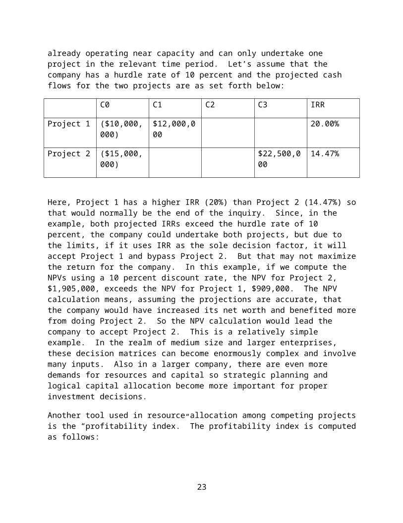
EXHIBIT A

23