Unemployment Insurance and the Role of Self-Insurance

Review of Economic Dynamics 5, 681–703 (2002)doi:10.1006/redy.2002.0159

Unemployment Insurance andthe Role of Self-Insurance1

Atila Abdulkadiroglu

Department of Economics, Columbia University, New York, New York 10027E-mail: [email protected]

Burhanettin Kurusçu

Department of Economics, University of Rochester, Rochester, New York 14627E-mail: [email protected]

and

Aysegul Sahin

Department of Economics, University of Rochester, Rochester, New York 14627E-mail: [email protected]

Received January 26, 2001; published online April 3, 2002

This paper employs a dynamic general equilibrium model to design and evaluatelong-term unemployment insurance plans (plans that depend on workers’ unem-ployment history) in economies with and without hidden savings. We show thatoptimal benefit schemes and welfare implications differ considerably in these twoeconomies. Switching to long-term plans can improve welfare significantly in theabsence of hidden savings. However, welfare gains are much lower when we con-sider hidden savings. Therefore, we argue that switching to long-term plans shouldnot be a primary concern from a policy point of view. Journal of Economic LiteratureClassification Numbers: J65, D82. 2002 Elsevier Science (USA)

Key Words: unemployment insurance; asymmetric and private information.

1We are grateful to Mark Bils and Per Krusell for their time and valuable comments.We also thank Jeremy Greenwood, Fatih Guvenen, Gary Hansen, Ayse Imrohoroglu, SeloImrohoroglu, two anonymous referees, and the conference participants at the MidwestMacroeconomics Conference 2000 and European Science Foundation Network Conferenceon Social Insurance: Modelling and Transition 2000 for their useful comments and sugges-tions. Any errors are our own.

681

1094-2025/02 $35.00 2002 Elsevier Science (USA)

All rights reserved.

682 abdulkadiroglu, kurusçu, and sahin

1. INTRODUCTION

An important adverse effect of unemployment insurance is the disincen-tive to find/maintain a job.2 Shavell and Weiss (1979) and Hopenhayn andNicolini (1997) suggest that a possible remedy is switching to long-termcontracts where benefit payments depend on workers’ unemployment his-tory. In particular, Hopenhayn and Nicolini (1997) show, by simulating asearch-theoretic model, that switching from the current U.S. unemploymentinsurance system to the optimal one may reduce the cost of the systemby 30%. The optimal plan they propose provides a declining benefit pathto create intertemporal incentives. It punishes workers (agents) for con-tinued unemployment and creates incentives to find a job. A maintainedassumption in these papers is that consumer/workers cannot save or, alter-natively, that any savings they undertake are perfectly monitored and thuscompletely controlled by the insurance provider. The main contribution ofour paper is to study long-term unemployment insurance plans by relaxingthe assumption that agents’ savings can be perfectly monitored. Thus, weconsider “hidden savings.” We believe that introducing hidden savings isimportant for at least two reasons. First, it is not realistic that perfect mon-itoring is available at zero cost. Second, and more important, if savings can-not be monitored, the incentives of consumer/workers change significantly.Suppose that we apply the unemployment insurance system suggested byShavell and Weiss (1979) and Hopenhayn and Nicolini (1997) to our econ-omy where agents have hidden savings. Then the agents would be temptedto cheat: they would try to get a higher net present value transfer from theunemployment insurance system and would deal with any implied increasein risk by self-insuring using their hidden savings. Thus, in an economy withhidden savings—where agents can self-insure—the government-providedinsurance may be less important and may change in nature.We find that indeed it is important to consider hidden savings in the

analysis. The nature of the optimal unemployment insurance plans dif-fers significantly from the ones suggested by Shavell and Weiss (1979) andHopenhayn and Nicolini (1997): the benefit path is not necessarily declin-ing. We also find that the role of history dependence of unemploymentinsurance plans is not as important quantitatively as the earlier studies sug-gest. Our analysis, in fact, also suggests that unemployment plans that aredesigned ignoring agents’ ability to save secretly could cause an increase inunemployment and be harmful to the economy.

2Hamermesh (1977), Moffitt (1985), and Meyer (1990) estimate that a 10% rise in thereplacement ratio might cause a 1

2 - to 1-week increase in the length of unemployment spell.Meyer (1990) predicts that a 10% increase in benefits leads to an 8.8% decrease in the prob-ability of leaving unemployment.

unemployment insurance 683

The model we study is different from the models analyzed in the citedpapers in several aspects. First of all, we do not look at fully optimal dynamiccontracts since they are difficult to characterize when agents have hiddensavings. However, we consider a broad set of history-dependent unemploy-ment insurance plans. Second, we focus on the moral hazard problem basedon unobservability of job refusals as opposed to the job-search effort as inShavell and Weiss (1979) and Hopenhayn and Nicolini (1997). Third, weinsist on budget balance of the unemployment insurance system. That is,there is a feedback of the benefit part of the system to the tax on the laborincome of employed agents. Therefore, we choose a dynamic general equi-librium model for our analysis.We study an extension of the model with incomplete markets analyzed in

Hansen and Imrohoroglu (1992). To understand the role of hidden savings,we also consider a variant of our model in which we shut down the savingschannel. The economy consists of ex-ante identical agents who derive utilityfrom consumption and leisure. Agents are subject to unemployment risk:at the beginning of each period, they are offered an employment opportu-nity with a certain probability. They can partially insure themselves againstthe possibility of income loss by saving through non-interest-bearing assets.Agents also have access to an unemployment insurance system financedby the government through proportional taxes. The system distinguishesagents according to their unemployment history: agents are offered differ-ent benefit levels, depending on how long they have been unemployed. Weintroduce moral hazard to the model by assuming that government mon-itoring of insurance claimants is imperfect; i.e., the government monitorsonly a certain fraction of the claimants. Therefore, agents who are notqualified (who refuse job opportunities) can collect benefits with a positiveprobability. We refer to imperfect government monitoring as moral hazard,because ineligible agents are more likely to take advantage of the unem-ployment insurance system when the government monitors a small fractionof claimants.In this framework, our objective is to compute the unemployment insur-

ance (UI) plans that maximize the steady-state equilibrium welfare. Oneshould consider all possible employment histories to find “the” optimal UIplan in the context of dynamic contracting literature. However, due to thecomputational complexity of this problem, we restrict our attention to acertain degree of history dependence. The unemployment insurance plansthat we consider focus only on the most recent unemployment spell anddistinguish agents with respect to the number of periods they have beenunemployed consecutively up to “T” periods. We allow the benefit levels tobe flexible for T periods and thereafter the benefit level is held constant. Weincrease T up to a point beyond which increasing T does not improve wel-fare significantly. We refer to the plan that maximizes steady-state average


utility as the optimal UI plan. We use a variant of the evolutionary algo-rithms suggested by Gomme (1997) to compute the optimal UI plans. Thisalgorithm reduces computation time drastically and makes it possible tosolve otherwise infeasible optimization problems.In this study, we analyze unemployment insurance in two different eco-

nomic environments. In the first economy, agents have hidden savings andin the second, they do not. Our analysis suggests that optimal benefit pathsdiffer remarkably in these two economies. In general, the optimal bene-fit levels are significantly higher and the optimal unemployment insuranceplan implies a declining benefit path when there are no savings. However,when agents have hidden savings, the optimal benefit path is not necessar-ily declining. Depending on the degree of moral hazard, the benefit pathcan be nonmonotonic or even increasing. Yet, the optimal unemploymentinsurance plan implies a declining consumption path as Shavell and Weiss(1979) and Hopenhayn and Nicolini (1997) argue. We also show that wel-fare implications of long-term plans are different in these two economies.Our experiments suggest that long-term plans can improve welfare sig-nificantly in economies without savings. For example, the welfare gain ofswitching to long-term plans is 2.0133% of consumption.3 Yet, the welfaregains are much lower if we consider savings in the analysis. The welfaregain varies between 0.0325% and 0.1840%, depending on the degree ofmoral hazard.An important result of our analysis is that the welfare gains of switch-

ing to unemployment insurance plans that depend on the unemploymenthistory are quite small when agents have hidden savings. Even if the govern-ment can monitor a large fraction of unemployment claimants, the welfaregains are as low as 0.06%. We show that our conclusion is not affectedby plausible variations in parameters. Given our results and the fact thatlong-term unemployment insurance plans are hard to administer in prac-tice, we argue that switching to long-term plans perhaps should not be aprimary concern from a policy point of view.Finally, our findings reveal that unemployment insurance plans, designed

ignoring agents’ ability to save privately, could be harmful to the econ-omy. When we apply the optimal plan from the economy without savingsto our economy with hidden savings, a quite drastic increase in unemploy-ment results. This is because this plan critically uses history dependence;in particular, it applies high benefit rates in the first few periods uponjob loss. Thus, any recently separated workers with access to hidden sav-ings would choose to turn down new job offers, collect the high benefit,and use hidden savings to smooth consumption. This example also reveals

3Welfare gains are computed as a percentage of consumption.


the importance of taking into account the general equilibrium effects inthe design of unemployment insurance plans: the lower the employmentrate is, the higher the tax rate on labor income of the employed shouldbe in order to balance the budget of the unemployment insurance system.This feedback—which indeed is present in real life—exacerbates the neg-ative effects of improperly designed unemployment insurance systems onthe economy.Hansen and Imrohoroglu (1992) is the first study that analyzes the wel-

fare effects of the unemployment insurance system in a general equilibriumenvironment with moral hazard and savings. They concentrate on constantbenefit schemes and argue that it is almost impossible to insure agents forhigh degrees of moral hazard. We generalize their result by showing thatmore complicated unemployment insurance plans do not provide much bet-ter insurance when agents have hidden savings.Long-term unemployment insurance plans in environments where agents

have hidden savings are also studied by Wang and Williamson (1999).They evaluate alternative unemployment insurance schemes in a dynamiceconomy with unobservable job-search and job-retention effort. Theirmain concern is to study the welfare implications of long-term plans andexperience rating. They, too, report small welfare gains from switching tolong-term plans. It is noteworthy that they reach a similar conclusion toours by using a different framework. However, they do not specifically ana-lyze how savings affect the nature and the role of long-term unemploymentinsurance plans.The plan of the paper is as follows. In Section 2, we describe the econ-

omy. Section 3 discusses the calibration. Section 4 explains the algorithmused in the numerical solution. Section 5 discusses calculation of welfaregains. In Section 6, we present our results. Section 7 provides an exampleregarding the importance of hidden savings. Section 8 presents our conclu-sions.

2. THE ECONOMIC ENVIRONMENT

2.1. The Model Economy with Savings

We use a dynamic general equilibrium model with hidden savings toanalyze different unemployment insurance plans. The economy consists ofex-ante identical infinitely lived agents who derive utility from consumptionand leisure. Individuals maximize the expected value of their discountedutility

E∞∑j=0

βjU�cj� lj�� (1)


where β is the discount factor, U�·� ·� is the momentary utility function, cjis the consumption, and lj is the leisure. Each agent has one unit of timein each period that can be allocated between work and leisure. An agenteither chooses to work a fixed amount of h ∈ �0� 1� number of hours, andproduces y units of consumption goods or does not work at all.In this model, agents can save through non-interest-bearing assets but

they cannot borrow. Assets evolve according to

m′ = m+ yd − c� (2)

where m is the asset holdings in the current period, c is the consumptionin the current period, m′ is the asset holdings in the next period, and yd isthe disposable income in the current period.Agents are offered employment opportunities according to a stochastic

process. Let s denote the employment opportunity state of an individual. Ifs = e, the agent has a job offer and he or she chooses to accept or rejectthe offer. If s = u, he or she becomes unemployed.

Let η denote the employment status of the agent. If he or she chooses towork, η = 1; otherwise, η = 0. We can summarize the employment statusof the agent as

Job offer �s = e�−→{Accept → Work for h hours �η = 1��Reject → Unemployed �η = 0�,

No job offer �s = u�−→Unemployed �η = 0��(3)

It is assumed that s follows a two-state Markov chain. The transitionprobabilities are given by the 2 × 2 transition matrix χ = �χ�i� j�� wherei� j ∈ �e� u�. For instance, given that the agent did not have an employmentopportunity in the last period, the probability of getting a job offer in thecurrent period is Prob�s′ = e�s = u� = χ�u� e�.The unemployment history of an agent is denoted by t, the number of

periods he or she has been unemployed consecutively in the last unem-ployment spell. For example, if the agent has been unemployed for threeperiods, then t = 3.

Our insurance plan is characterized by a replacement ratio of the form

θ�t� ={θt� t ∈ �0� � � � � T − 1�,θT−1� t ≥ T . (4)

This UI plan distinguishes agents according to their unemployment his-tory up to t = T . For an unemployed agent, the replacement ratio is θ0 inthe first period of unemployment and θt−1 in the tth period up to the T thperiod. Thereafter, it will be constant at θT−1. When T = 1, the replace-ment ratio is constant. This case corresponds to the UI plans analyzed inHansen and Imrohoroglu (1992).


In our framework, agents who refuse job opportunities can collect UIbenefits with positive probability, π�t�. The degree of moral hazard iscontrolled by changing π�t�. Note that π�t� = 0 corresponds to perfectmonitoring, i.e., no moral hazard, and π�t� = 1 corresponds to no moni-toring, i.e., extreme moral hazard. We differentiate between the individualswho have worked last period and those who have not by letting

π�t� ={π0 for t = 0,π1 for t > 0 (5)

and assigning different values for π0 and π1.We can summarize the unemployment insurance system as follows:

• If the agent has no job offer (s = u), then he or she collects benefits.The amount of benefit is determined by the long-term UI plan according to(4). The current employment status is η = 0 and the unemployment historybecomes t ′ = t + 1.

• If the agent has a job offer (s = e) and he or she accepts it, then heor she does not receive any benefits. Then η = 1 and t ′ = 0.

• If the agent has a job offer (s = e) but he or she does not accept it,then he or she receives the UI benefit with probability π�t�. For this case,η = 0 and t ′ = t + 1.

Let µ be the indicator that shows whether an agent receives UI benefits.If the agent receives benefits, µ = 1; otherwise, µ = 0. Government usesproportional income tax to finance UI benefits. Let τ be the proportionalincome tax rate. The state of the agent can be summarized as

s = u� η = 0→ t ′ = t + 1� µ = 1� and yd = �1− τ�θ�t�y�s = e� η = 1→ t ′ = 0� µ = 0� and yd = �1− τ�y�

s = e� η = 0→ t ′ = t + 1�

µ = 1� and yd = �1− τ�θ�t�y

with probability π�t��µ = 0� and yd = 0

with probability 1− π�t��

(6)

The timing in the model is:

• At the beginning of each period, the employment opportunity states is known to agents. Given the employment opportunity s, asset holdingsm, and employment history t, they choose η.

• Agents who do not receive employment opportunities collect bene-fits with certainty and choose consumption and next period’s asset holdings.At the same time, agents who work choose consumption and next period’sasset holdings.


• Agents who reject employment opportunities first learn whether theyreceive benefits and then they choose consumption and next period’s assetholdings according to Eq. (2).

The maximization problem can be written as a dynamic programmingproblem. Note that the state variables are current asset holdings m, employ-ment opportunity s, and employment history t. The dynamic programmingproblem is

V �m�u�t� = maxm′

{U�m+�1−τ�θ�t�y−m′�1�

+β∑s′χ�u�s′�V �m′�s′�t+1�

}�

V �m�e�t� = max{maxm′

{U�m+�1−τ�y−m′�1−h�

+β∑s′χ�e�s′�V �m′�s′�0�

}�

π�t�[maxm′

{U�m+�1−τ�θ�t�y−m′�1�

+β∑s′χ�e�s′�V �m′�s′�t+1�

}]

+�1−π�t��[maxm′

{U�m−m′�1�

+β∑s′χ�e�s′�V �m′�s′�t+1�

}]}

(7)

subject to m′ ≥ 0.

Definition. The stationary equilibrium for this economy is the setof decision rules c�x��m′�x�, and η�m� s� t�, where x = �m� s� t� µ�, atime-invariant measure λ�x� of individuals at state x and a tax rate τ suchthat

1. Given the tax rate τ, individuals solve the maximization problemin (7).

2. The goods market clears:∑x

λ�x�c�x� = ∑x

λ�x�η�x�y� (8)

3. Government finances UI benefits by taxing income. So, the totalamount of UI benefits should be equal to the taxes paid by the employedindividuals. The government budget constraint is satisfied:∑

m� t

λ�m� e� t� 0�η�m� e� t�τy

= ∑m� t

[λ�m�u� t� 1� + λ�m� e� t� 1�]�1− τ�θ�t�y� (9)


4. The invariant measure λ�x� solves the equation

λ�m′� s′� t ′� µ′�

=

0� s′ = u�µ′ = 0,

∑s

∑µ

∑�m� t�∈�

χ�s� s′�λ�x�� s′ = u�µ′ = 1,

∑s

∑µ

∑�m� t�∈�

χ�s� s′�λ�x�[η′�m′� s′� t ′�

+ (1− π�t ′�)�1− η′�m′� s′� t ′��]� s′ = e�µ′ = 0,

∑s

∑µ

∑�m� t�∈�

χ�s� s′�λ�x�

× [π�t ′�(1− η′�m′� s′� t ′�)]� s′ = e�µ′ = 1,

(10)

where ��m′� s� t ′� µ� = ��m� t� � m′ = m′�m� s� t� µ� and t ′ = �t + 1��1 −η�m� s� t��.The first part of Eq. (10) corresponds to the fraction of agents who have

no job offer and no unemployment benefits. Since every individual whodoes not get any job offer receives UI benefits, the fraction of such agentsis 0. The second part corresponds to the fraction of agents who have no joboffer and receive benefits. Since anybody without a job offer receives UIbenefits with certainty, this part is equal to the total fraction of individualswho have no job offer. The third part corresponds to the fraction of indi-viduals who have a job offer but do not receive UI benefits. These are theindividuals who decided to work or who rejected the job offer and did notreceive benefits.4 The fourth part corresponds to the fraction of individualswho rejected job offers and receive benefits.

2.2. The Model Economy without Savings

The economy without savings is a special case of the economy that weanalyzed in the previous section. We restrict asset holdings to be 0 in allperiods, i.e., m = m′ = 0. Since agents do not have any savings, the onlysource of consumption for the unemployed is UI benefits.

4Recall that the individuals who refuse job offers do not receive any benefits with probability1− π�t ′�.


3. CALIBRATION

• The utility function used in the computations has the form

U�c� l� = �c1−σlσ�1−ρ − 11− ρ � (11)

• The time period in the model is 6 weeks and output is normalizedto 1. Following Kydland and Prescott (1982), β is set to 0.995.

• h is set to 0.45, assuming that individuals have 98 hours in a week(when sleeping, eating, etc. are deducted) and they spend approximately 45hours of this time at work.

• σ is set to 0.67 in our benchmark parameterization, followingKydland and Prescott (1982). However, Acemoglu and Shimer (2000) sug-gest smaller values for σ . So we check the robustness of our results bychanging σ to 0.5.

• The degree of risk aversion ρ is set to 2.5, following Mehra andPrescott (1985) in the benchmark case. We also examine how our resultsare affected when ρ = 10.

• Following Hansen and Imrohoroglu (1992), the transition matrix χis formed such that the employment opportunity is offered 94% of the timeand the average duration of not having an employment opportunity is 12weeks. These requirements imply that the transition matrix is[

χ�e� e� χ�e� u�χ�u� e� χ�u� u�

]=

[0�9681 0�03190�5000 0�5000

]� (12)

• We set π1 = 1 and consider different levels of monitoring of quittersand change π0 from 0 to 1.

4. COMPUTATION

We want to compute average utility for different T = �θ�0�� θ�1��θ�2�� θ�T − 1�� θ�T �� sequences to find the optimal benefitscheme.The computational procedure for a given T is as follows:

1. Start with a guess for tax rate τ and solve the dynamic program-ming problem by value function iteration:

a. Form a discrete state space for (m� s� t). Note that m is allowedto take values between 0 and 8 and a grid of 301 points is used. Since s cantake only two values and t can take T values, the dimension of the statespace is 301× 2 × T .


b. Start with an initial guess V 0�·� ·� ·� for V �·� ·� ·�.c. Calculate V n+1�·� ·� ·� by value function iteration.d. Repeat step c until the value function converges.

2. Calculate λ�x� by iterating on Eq. (9):a. Start with an initial guess for λ�x�.b. Calculate an updated λ�x� by using Eq. (9).c. Repeat this procedure until convergence.

3. Calculate the budget constraint by using Eq. (7). If there is a sur-plus (deficit), decrease (increase) the tax rate.

4. Steps 1–4 are repeated until the equilibrium is found.

The above procedure calculates the decision rules and tax rate for a given T sequence. Our goal is to find the optimal UI plan. Calculation of theoptimal UI plan requires repetition of the above procedure for all possible T sequences. In our computations, θ is allowed to take values between0 and 1 and a grid of 21 points is used. For T = 1, the number of allpossible UI plans is just 21, but as T increases, the number of possible UIplans increases dramatically. For example, for T = 4, we need to repeatthe solution procedure 214 = 194�481 times. The dramatic increase in thecomputation time with increasing T makes the direct solution impossible.Following Gomme (1997), we use an evolutionary algorithm to find theoptimal θT sequence:

1. Construct a population of 20 T sequences as first guesses.2. For each T sequence in the population, calculate the average

utility in the equilibrium by using the above algorithm.3. Sort the population from the best to the worst according to the

corresponding values of average utility.4. Replace the worst half of the population by the first half of the

population by adding some random noise.5. Repeat steps 2–5 with the new population until all of the top 10

T sequences are the same.

The noise added in step 4 helps the evolutionary algorithm to escape fromlocal minima and, at the same time, explore the space of all possible T

sequences.

5. SOCIAL PLANNER’S PROBLEM ANDCALCULATION OF WELFARE GAINS

In the following sections, we are going to evaluate equilibrium alloca-tions under different UI plans. For this purpose, we solve a social planner’s


problem and evaluate the gap between the social planner’s allocation andthe equilibrium allocation under a certain plan. The social planner’s allo-cation is given by the solution to

max∞∑t=0

βt[NtU�c1t � 1− h� + �1−Nt�U�c2t � 1�

](13)

subject to

Ntc1t + �1−Nt�c2t ≤ Nty� Nt ≤ �N�where Nt is the employment rate, c1t is the consumption of an employedindividual, and c2t is the consumption of an unemployed individual. �N is theupper bound on the employment rate which was set to 0.94. This problem isstatic in nature and has a simple closed-form solution as shown in Hansenand Imrohoroglu (1992). Let (c∗1� c

∗2) be the solution to the problem above.

To compute the welfare cost of an equilibrium allocation, we calculate theaverage utility, V , under that particular allocation. Then we compute thevalue of φ such that the allocation (φc∗1� φc

∗2) gives the utility V ; the welfare

cost is given by 1−φ.

6. DESIGN AND EVALUATION OF OPTIMAL UI PLANS

In this section, we examine optimal UI plans in two different economicenvironments. These two sample economies are identical except for the dis-tinction that, in the first one, agents cannot save and, in the second one,they can. We compute optimal unemployment insurance plans for differentlevels of government monitoring. We distinguish between agents accord-ing to the number of periods they have been unemployed up to T periodsand find the optimal benefit schemes by varying T from 1 to 4. We eval-uate potential welfare gains of going from T = 1 to T = 4. Recall thatT = 1 corresponds to the case where the benefits are constant throughoutthe unemployment spell (short-term unemployment insurance plans), andT > 1 corresponds to the case with a changing benefit level throughout theunemployment spell (long-term plans).5

In the following section, we present results for π1 = 1. This situationin which it is not possible to monitor searchers seems to be empiricallyplausible given the fact that search activity is hard to monitor. Although

5We have tried increasing T to 5 and seen that distinguishing agents beyond the fourthperiod of unemployment does not improve welfare significantly. Given this and the computa-tional complexity of solving the problem for higher values of T , we carry out our analysis upto T = 4.


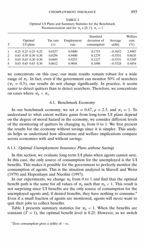
TABLE IOptimal UI Plans and Summary Statistics for the Benchmark

Parameterization and for π0 ∈ �0� 1�, π1 = 1

Standard WelfareOptimal Tax rate Employment deviation of Average cost

T UI plans �τ� rate consumption utility (%)

1 0.25 0.25 0.25 0.25 0.0157 0.9400 0.1753 −0�5652 2.49872 0.65 0.30 0.30 0.30 0.0294 0.9400 0.1279 −0�5551 0.86353 0.65 0.65 0.30 0.30 0.0445 0.9253 0.1127 −0�5531 0.53494 0.65 0.65 0.65 0.30 0.0612 0.9044 0.1098 −0�5528 0.4854

we concentrate on this case, our main results remain robust for a widerange of π1. In fact, even if the government can monitor 50% of searchers�π1 = 0�5�, our results do not change significantly. In practice, it seemseasier to detect quitters than to detect searchers. Therefore, we concentrateon cases where π0 < π1.

6.1. Benchmark Economy

In our benchmark economy, we set σ = 0�67� ρ = 2�5, and π1 = 1. Tounderstand to what extent welfare gains from long-term UI plans dependon the degree of moral hazard in the economy, we consider different levelsof the monitoring of quitters by changing π0 from 0 to 1. We first presentthe results for the economy without savings since it is simpler. This analy-sis helps us understand how allocations and welfare implications compareacross economies with and without savings.

6.1.1. Optimal Unemployment Insurance Plans without Savings

In this section, we evaluate long-term UI plans when agents cannot save.In this case, the only source of consumption for the unemployed is the UIbenefits. This makes it possible for the government to perfectly monitor theconsumption of agents. This is the situation analyzed in Shavell and Weiss(1979) and Hopenhayn and Nicolini (1997).In our experiments, we change π0 from 0 to 1 and find that the optimal

benefit path is the same for all values of π0 such that π0 < 1. This result isnot surprising since UI benefits are the only source of consumption for theunemployed agents and, if denied benefits, they have nothing to consume.6

Even if a small fraction of agents are monitored, agents will never want toquit their jobs to collect benefits.Table I presents summary statistics for π0 < 1. When the benefits are

constant (T = 1), the optimal benefit level is 0.25. However, as we switch

6Zero consumption gives a utility of −∞.


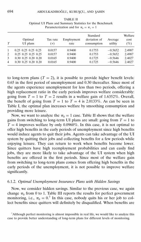
TABLE IIOptimal UI Plans and Summary Statistics for the Benchmark

Parameterization and for π0 = π1 = 1

Standard WelfareOptimal Tax rate Employment deviation of Average cost

T UI plans �τ� rate consumption utility (%)

1 0.25 0.25 0.25 0.25 0.0157 0.9400 0.1753 −0�5652 2.49872 0.25 0.25 0.25 0.25 0.0157 0.9400 0.1753 −0�5652 2.49873 0.30 0.25 0.20 0.20 0.0165 0.9400 0.1725 −0�5646 2.40274 0.30 0.25 0.20 0.20 0.0165 0.9400 0.1725 −0�5646 2.4027

to long-term plans (T = 2), it is possible to provide higher benefit levels:0.65 in the first period of unemployment and 0.30 thereafter. Since most ofthe agents experience unemployment for less than two periods, offering ahigh replacement ratio in the early periods improves welfare considerably:going from T = 1 to T = 2 results in a welfare gain of 1.6352%. Overall,the benefit of going from T = 1 to T = 4 is 2.0133%. As can be seen inTable I, the optimal plan increases welfare by smoothing consumption andproviding more leisure.Now, we want to analyze the π0 = 1 case. Table II shows that the welfare

gains from switching to long-term UI plans are small: going from T = 1 toT = 4 improves welfare by only 0.0960%. In this case, it is not optimal tooffer high benefits in the early periods of unemployment since high benefitswould induce agents to quit their jobs. Agents can take advantage of the UIsystem by quitting their jobs and collecting benefits for a few periods whileenjoying leisure. They can return to work when benefits become lower.Since quitters have high reemployment probabilities and can easily findjobs, they are more likely to take advantage of the UI system when highbenefits are offered in the first periods. Since most of the welfare gainfrom switching to long-term plans comes from offering high benefits in theearly periods of the unemployment, it is not possible to improve welfaresignificantly.

6.1.2. Optimal Unemployment Insurance Plans with Hidden Savings

Now, we consider hidden savings. Similar to the previous case, we againchange π0 from 0 to 1. Table III reports the results for perfect governmentmonitoring, i.e., π0 = 0.7 In this case, nobody quits his or her job to col-lect benefits since quitters will definitely be disqualified. When benefits are

7Although perfect monitoring is almost impossible in real life, we would like to analyze thiscase to provide better understanding of long-term plans for different levels of monitoring.


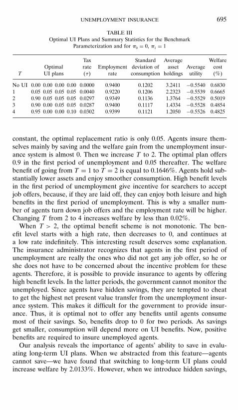
TABLE IIIOptimal UI Plans and Summary Statistics for the Benchmark

Parameterization and for π0 = 0, π1 = 1

Tax Standard Average WelfareOptimal rate Employment deviation of asset Average cost

T UI plans �τ� rate consumption holdings utility (%)

No UI 0.00 0.00 0.00 0.00 0.0000 0.9400 0.1202 3.2411 −0�5540 0.68301 0.05 0.05 0.05 0.05 0.0040 0.9220 0.1206 2.2323 −0�5539 0.66652 0.90 0.05 0.05 0.05 0.0297 0.9349 0.1136 1.3764 −0�5529 0.50193 0.90 0.00 0.05 0.05 0.0287 0.9400 0.1117 1.4334 −0�5528 0.48544 0.95 0.00 0.00 0.10 0.0302 0.9399 0.1121 1.2050 −0�5526 0.4825

constant, the optimal replacement ratio is only 0.05. Agents insure them-selves mainly by saving and the welfare gain from the unemployment insur-ance system is almost 0. Then we increase T to 2. The optimal plan offers0.9 in the first period of unemployment and 0.05 thereafter. The welfarebenefit of going from T = 1 to T = 2 is equal to 0.1646%. Agents hold sub-stantially lower assets and enjoy smoother consumption. High benefit levelsin the first period of unemployment give incentive for searchers to acceptjob offers, because, if they are laid off, they can enjoy both leisure and highbenefits in the first period of unemployment. This is why a smaller num-ber of agents turn down job offers and the employment rate will be higher.Changing T from 2 to 4 increases welfare by less than 0.02%.When T > 2, the optimal benefit scheme is not monotonic. The ben-

efit level starts with a high rate, then decreases to 0, and continues ata low rate indefinitely. This interesting result deserves some explanation.The insurance administrator recognizes that agents in the first period ofunemployment are really the ones who did not get any job offer, so he orshe does not have to be concerned about the incentive problem for theseagents. Therefore, it is possible to provide insurance to agents by offeringhigh benefit levels. In the latter periods, the government cannot monitor theunemployed. Since agents have hidden savings, they are tempted to cheatto get the highest net present value transfer from the unemployment insur-ance system. This makes it difficult for the government to provide insur-ance. Thus, it is optimal not to offer any benefits until agents consumemost of their savings. So, benefits drop to 0 for two periods. As savingsget smaller, consumption will depend more on UI benefits. Now, positivebenefits are required to insure unemployed agents.Our analysis reveals the importance of agents’ ability to save in evalu-

ating long-term UI plans. When we abstracted from this feature—agentscannot save—we have found that switching to long-term UI plans couldincrease welfare by 2.0133%. However, when we introduce hidden savings,


TABLE IVOptimal UI Plans and Welfare Gains for the Benchmark Parameterization

and for π1 = 1, π0 ∈ �0� 0�1� 0�25� 0�5� 1�

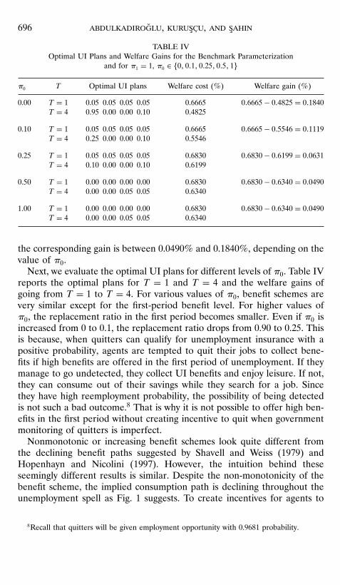
π0 T Optimal UI plans Welfare cost (%) Welfare gain (%)

0.00 T = 1 0.05 0.05 0.05 0.05 0.6665 0�6665− 0�4825 = 0�1840T = 4 0.95 0.00 0.00 0.10 0.4825

0.10 T = 1 0.05 0.05 0.05 0.05 0.6665 0�6665− 0�5546 = 0�1119T = 4 0.25 0.00 0.00 0.10 0.5546

0.25 T = 1 0.05 0.05 0.05 0.05 0.6830 0�6830− 0�6199 = 0�0631T = 4 0.10 0.00 0.00 0.10 0.6199

0.50 T = 1 0.00 0.00 0.00 0.00 0.6830 0�6830− 0�6340 = 0�0490T = 4 0.00 0.00 0.05 0.05 0.6340

1.00 T = 1 0.00 0.00 0.00 0.00 0.6830 0�6830− 0�6340 = 0�0490T = 4 0.00 0.00 0.05 0.05 0.6340

the corresponding gain is between 0.0490% and 0.1840%, depending on thevalue of π0.

Next, we evaluate the optimal UI plans for different levels of π0. Table IVreports the optimal plans for T = 1 and T = 4 and the welfare gains ofgoing from T = 1 to T = 4. For various values of π0, benefit schemes arevery similar except for the first-period benefit level. For higher values ofπ0, the replacement ratio in the first period becomes smaller. Even if π0 isincreased from 0 to 0.1, the replacement ratio drops from 0.90 to 0.25. Thisis because, when quitters can qualify for unemployment insurance with apositive probability, agents are tempted to quit their jobs to collect bene-fits if high benefits are offered in the first period of unemployment. If theymanage to go undetected, they collect UI benefits and enjoy leisure. If not,they can consume out of their savings while they search for a job. Sincethey have high reemployment probability, the possibility of being detectedis not such a bad outcome.8 That is why it is not possible to offer high ben-efits in the first period without creating incentive to quit when governmentmonitoring of quitters is imperfect.Nonmonotonic or increasing benefit schemes look quite different from

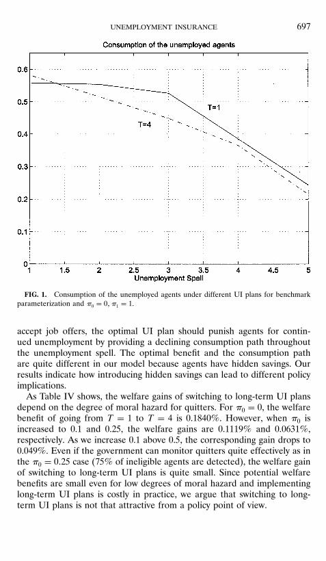
the declining benefit paths suggested by Shavell and Weiss (1979) andHopenhayn and Nicolini (1997). However, the intuition behind theseseemingly different results is similar. Despite the non-monotonicity of thebenefit scheme, the implied consumption path is declining throughout theunemployment spell as Fig. 1 suggests. To create incentives for agents to

8Recall that quitters will be given employment opportunity with 0.9681 probability.


FIG. 1. Consumption of the unemployed agents under different UI plans for benchmarkparameterization and π0 = 0� π1 = 1.

accept job offers, the optimal UI plan should punish agents for contin-ued unemployment by providing a declining consumption path throughoutthe unemployment spell. The optimal benefit and the consumption pathare quite different in our model because agents have hidden savings. Ourresults indicate how introducing hidden savings can lead to different policyimplications.As Table IV shows, the welfare gains of switching to long-term UI plans

depend on the degree of moral hazard for quitters. For π0 = 0, the welfarebenefit of going from T = 1 to T = 4 is 0.1840%. However, when π0 isincreased to 0.1 and 0.25, the welfare gains are 0.1119% and 0.0631%,respectively. As we increase 0.1 above 0.5, the corresponding gain drops to0.049%. Even if the government can monitor quitters quite effectively as inthe π0 = 0�25 case (75% of ineligible agents are detected), the welfare gainof switching to long-term UI plans is quite small. Since potential welfarebenefits are small even for low degrees of moral hazard and implementinglong-term UI plans is costly in practice, we argue that switching to long-term UI plans is not that attractive from a policy point of view.


TABLE VOptimal UI Plans and Welfare Gains for σ = 0�5, π0 ∈ �0� 1�, and π1 = 1

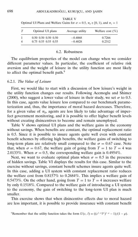
T Optimal UI plans Average utility Welfare cost (%)

1 0.50 0.50 0.50 0.50 −0�4068 0.72664 0.75 0.55 0.55 0.55 −0�4028 0.2312

6.2. Robustness

The equilibrium properties of the model can change when we considerdifferent parameter values. In particular, the coefficient of relative riskaversion and the weight of leisure in the utility function are most likelyto affect the optimal benefit path.9

6.2.1. The Value of Leisure

First, we would like to start with a discussion of how leisure’s weight inthe utility function changes our results. Following Acemoglu and Shimer(2000), who suggest a lower value of leisure in their study, we set σ to 0.5.In this case, agents value leisure less compared to our benchmark parame-terization and, thus, the importance of moral hazard decreases. Therefore,for a given value of π0, agents are less likely to take advantage of imper-fect government monitoring, and it is possible to offer higher benefit levelswithout creating disincentives to become and remain unemployed.Table V shows optimal UI plans and the welfare gains in the economy

without savings. When benefits are constant, the optimal replacement ratiois 0.5. Since it is possible to insure agents quite well even with constantbenefit schemes by offering high benefits, the welfare gains of switching tolong-term plans are relatively small compared to the σ = 0�67 case. Notethat, when σ = 0�67, the welfare gain of going from T = 1 to T = 4 was2.0133%. When σ = 0�5, the corresponding welfare gain is 0.4954%.Next, we want to evaluate optimal plans when σ = 0�5 in the presence

of hidden savings. Table VI displays the results for this case. Similar to theexercise without savings, constant benefit schemes insure agents quite well.In this case, adding a UI system with constant replacement ratio reducesthe welfare cost from 0.8157% to 0.2684%. This implies a welfare gain of0.5473%. On the other hand, going from T = 1 to T = 4 increases welfareby only 0.1518%. Compared to the welfare gain of introducing a UI systemto the economy, the gain of switching to the long-term UI plan is muchsmaller.This exercise shows that when disincentive effects due to moral hazard

are less important, it is possible to provide insurance with constant benefit

9Remember that the utility function takes the form U�c� l� = ��c1−σ lσ�1−ρ − 1�/�1− ρ�.


TABLE VIOptimal UI Plans and Summary Statistics for σ = 0�5� π0 ∈ �0� 0�5�, and π1 = 1


No UI 0.00 0.00 0.00 0.00 −0�4075 0.81571 0.45 0.45 0.45 0.45 −0�4039 0.26844 1.00 0.40 0.45 0.50 −0�4019 0.1166

schemes. Therefore, the welfare gains of switching to long-term UI plansare relatively small as we have discussed above.

6.2.2. Risk Aversion

Next, we want to describe the behavior of the economy when a higherdegree of risk aversion is assumed. When risk aversion is higher, agentsprefer smoother consumption of the composite commodity, c1−σlσ .

Table VII displays the results for ρ = 10 in the economy without savings.Compared to our benchmark case, replacement rates are lower in gen-eral and benefit schemes are flatter. Since more risk-averse agents prefersmoother consumption of the composite commodity, benefit levels shouldbe lower to provide a smoother utility. If the replacement rate were higher,the utility of an unemployed agent would be much higher than that of anemployed agent.10

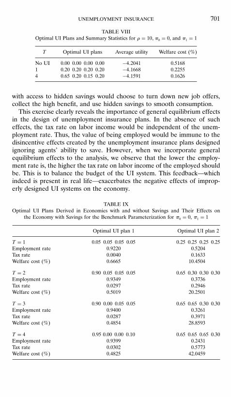
Finally, we want to describe the behavior of the economy with hidden sav-ings for ρ = 10. Table VIII displays the results. Compared to the ρ = 2�5case, benefit levels are generally higher and benefit paths are flatter. Theseresults follow from the fact that more risk-averse agents prefer smootherconsumption of the composite commodity, c1−σlσ . When the replacementratio is constant, the optimal level is 0.2. Recall that, when ρ = 2�5, thecorresponding replacement ratio was 0.05, implying a much smaller com-posite commodity for the unemployed. Then the only way to smooth theconsumption of the composite commodity is to increase the consumptionof goods �c� since leisure for the unemployed is already high. That is whybenefit levels are higher when agents are more risk averse. The reason thatlong-term plans are flatter compared to the benchmark case is also verysimilar: since every unemployed agent enjoys the same amount of leisure,the only way to provide a smoother utility flow over the unemployment

10When ρ = 2�5, the replacement ratio in the first few periods of unemployment is 0.65.Then the amount of composite commodity consumed by the unemployed agent will be0�650�3310�67 = 0�8675. For the employed agent, the consumption is around 0.94 and leisureis 0.55. Then the composite commodity of the employed agent is 0�940�330�550�67 = 0�6564.Note that the instantaneous utility of the unemployed agent is higher.


TABLE VIIOptimal UI Plans and Welfare Gains for ρ = 10� π0 = 0, and π1 = 1


1 0.25 0.25 0.25 0.25 −4�3442 1.58084 0.40 0.30 0.30 0.25 −4�1899 0.4061

spell is to provide a lower benefit level in the first period of unemploymentand higher benefit levels in the later periods.11

For ρ = 10, when we introduce an unemployment insurance system with aconstant benefit level, the welfare cost is reduced from 0.5168% to 0.2255%.This implies a welfare gain of 0.2913%. However, using long-term plansdoes not improve welfare significantly: as we go from T = 1 to T = 4, theimprovement in welfare is only 0.0629%.12

7. ROLE OF SAVINGS

Our experiments show that policy implications change considerably whenhidden savings are taken into account. UI plans designed without consider-ing savings can cause high unemployment and be quite harmful if appliedto an economy with hidden savings. This section illustrates this argumentquantitatively. We compare the employment rates for the economy with hid-den savings when (a) the optimal UI plans suggested by the same economyare applied and (b) the optimal UI plans suggested by the economy withoutsavings are applied. Table IX shows that if UI plans are designed withoutconsidering hidden savings, they might be quite harmful to the economy.For example, for T = 1 the employment rate decreases from 92% to 52%and the welfare cost increases from 0.6665% to 10.4504%. It is remark-able that the long-term UI plans suggested by the economy without savingscause even higher unemployment rates and higher welfare cost. For exam-ple, for T = 4 the employment rate decreases from 94% to 24.3% and thewelfare cost increases from 0.4825% to 42.0459%. This is because this plancritically uses history dependence; in particular, it applies high benefit ratesin the first few periods upon job loss. Thus, any recently separated workers

11When ρ = 2�5, the optimal benefit scheme for T = 4 is (0.95, 0, 0, 0.10); when ρ = 10,the optimal benefit scheme is (0.65, 0.20, 0.15, 0.20).

12When we tried higher values of π0, we noticed that the optimal benefit level for T = 1does not change significantly. For instance, when π0 = 0�5, the constant benefit scheme stilloffers 0.20. So, the welfare benefit of introducing a UI plan is 0.2913%. However, higherlevels of moral hazard decrease the welfare benefit of switching to long-term plans. Thus, thewelfare gains will be less than 0.0629%.


TABLE VIIIOptimal UI Plans and Summary Statistics for ρ = 10� π0 = 0, and π1 = 1


No UI 0.00 0.00 0.00 0.00 −4�2041 0.51681 0.20 0.20 0.20 0.20 −4�1668 0.22554 0.65 0.20 0.15 0.20 −4�1591 0.1626

with access to hidden savings would choose to turn down new job offers,collect the high benefit, and use hidden savings to smooth consumption.This exercise clearly reveals the importance of general equilibrium effects

in the design of unemployment insurance plans. In the absence of sucheffects, the tax rate on labor income would be independent of the unem-ployment rate. Thus, the value of being employed would be immune to thedisincentive effects created by the unemployment insurance plans designedignoring agents’ ability to save. However, when we incorporate generalequilibrium effects to the analysis, we observe that the lower the employ-ment rate is, the higher the tax rate on labor income of the employed shouldbe. This is to balance the budget of the UI system. This feedback—whichindeed is present in real life—exacerbates the negative effects of improp-erly designed UI systems on the economy.

TABLE IXOptimal UI Plans Derived in Economies with and without Savings and Their Effects on

the Economy with Savings for the Benchmark Parameterization for π0 = 0, π1 = 1

Optimal UI plan 1 Optimal UI plan 2

T = 1 0.05 0.05 0.05 0.05 0.25 0.25 0.25 0.25Employment rate 0.9220 0.5204Tax rate 0.0040 0.1633Welfare cost (%) 0.6665 10.4504





8. CONCLUSION

We have studied short-term and long-term unemployment insuranceplans in economies with and without savings. We find that welfare implica-tions change notably when we consider savings. Although long-term planscan improve welfare significantly in economies without savings, our experi-ments suggest that welfare gains are much lower when hidden savings aretaken into account.Potential welfare gains of long-term plans depend on the degree of moral

hazard. However, for a wide range of moral hazard values, we find thatthe welfare gains of long-term unemployment insurance plans are closeto 0. Our conclusion is not affected by plausible variations in parameters,including the coefficient of relative risk aversion and the weight of leisurein the utility function.We recognize that our results are not strictly comparable to those of the

dynamic contracting literature since our plans do not keep track of theentire unemployment history of workers. One might argue that contractsthat depend only on the most recent unemployment spell and distinguishagents up to four periods can be considered short-term contracts. However,we have shown that these contracts, in fact, improve welfare considerablyin economies without savings. This result suggests that the small welfaregains we obtain with hidden savings are not a consequence of limited his-tory dependence but rather a consequence of hidden savings. Given theseresults, as well as the fact that long-term unemployment insurance plansare hard to administer in practice, switching to long-term plans may not bea desirable policy.

REFERENCES

Acemoglu, Daron, and Shimer, Robert. (2000). “Productivity Gains from UnemploymentInsurance,” European Economic Review 44, 1195–1224.

Gomme, Paul. (1997). “Evolutionary Programming as a Solution Technique for the BellmanEquation,” NBER Working Paper 9816.

Hamermesh, Daniel S. (1977). Jobless Pay and the Economy, Baltimore: Johns Hopkins Press.Hansen, Gary D., and Imrohoroglu, Ayse. (1992). “The Role of Unemployment Insurance in

an Economy with Liquidity Constraints and Moral Hazard,” Journal of Political Economy100, 118–142.

Hopenhayn, Hugo, and Nicolini, Juan Pablo. (1997). “Optimal Unemployment Insurance,”Journal of Political Economy 105, 412–418.

Kydland, Finn E., and Prescott, Edward C. (1982). “Time to Build and Aggregate Fluctua-tions,” Econometrica 50, 1345–1370.

Mehra, Rajnish, and Prescott, Edward C. (1985). “The Equity Premium: A Puzzle,” Journalof Monetary Economics 15, 145–161.


Meyer, Bruce D. (1990). “Unemployment Insurance and Unemployment Spells,” Econometrica58, 757–782.

Moffitt, Robert. (1985). “Unemployment Insurance and the Distribution of UnemploymentSpells,” Journal of Econometrics 28, 85–101.

Shavell, Steven, and Weiss, Laurence. (1979). “The Optimal Payment of Unemployment Insur-ance Benefits over Time,” Journal of Political Economy 87, 1347–1362.

Wang, Cheng, and Williamson, Stephen. (1999). “Moral Hazard, Optimal UnemploymentInsurance, and Experience Rating,” unpublished manuscript.

Unemployment Insurance and the Role of Self-Insurance

Documents

Transcript of Unemployment Insurance and the Role of Self-Insurance