Understanding Analysis of Variance

STAT COE-Report-29-2017

STAT Center of Excellence 2950 Hobson Way – Wright-Patterson AFB, OH 45433

Understanding Analysis of Variance

Best Practice

Authored by: Cory Natoli

21 December 2017

Revised 24 September 2018

The goal of the STAT COE is to assist in developing rigorous, defensible test

strategies to more effectively quantify and characterize system performance

and provide information that reduces risk. This and other COE products are

available at www.afit.edu/STAT.

http://www.afit.edu/STAT


Table of Contents

Executive Summary ....................................................................................................................................... 2

Introduction .................................................................................................................................................. 2

Method ......................................................................................................................................................... 3

One-Way ANOVA ...................................................................................................................................... 3

Motivating example .............................................................................................................................. 3

Model .................................................................................................................................................... 3

Model Building ...................................................................................................................................... 3

Assumptions .......................................................................................................................................... 4

Hypotheses ........................................................................................................................................... 4

Test Statistic .......................................................................................................................................... 5

Decision ................................................................................................................................................. 7

Multifactor ANOVA ................................................................................................................................... 8

Motivating example .............................................................................................................................. 8

Model .................................................................................................................................................... 8

Hypotheses ........................................................................................................................................... 9

Decision ................................................................................................................................................. 9

Example ............................................................................................................................................... 10

R Code ..................................................................................................................................................... 11

JMP .......................................................................................................................................................... 14

Conclusion ................................................................................................................................................... 16

References .................................................................................................................................................. 17

Revision 1, 24 Sep 2018: Formatting and minor typographical/grammatical edits.


Page 2

Executive Summary An important step in the DOE process is determining which factors truly affect the (numeric) response

variable. A solution to this problem is through the use of analysis of variance (ANOVA). ANOVA is a

procedure that uses hypothesis testing to determine whether the factor effects of two or more factors

are the same. This paper seeks to explain the basic statistical theory behind one-way ANOVA, as well as

detail the process and how to utilize ANOVA conceptually. Code is provided to perform ANOVA in R and

JMP.

Keywords: ANOVA, DOE, statistically significant, hypothesis testing, R, JMP

Introduction Analysis of Variance (ANOVA) is a common technique for analyzing the statistical significance of a

number of factors in a model. The overall goal of ANOVA is to select a model that only contains terms

that add valuable insight in determining the value of the response, or in other words, a model that only

includes statistically significant terms. Assuming the data comes from a designed experiment, the

analysis will answer the question “Does this (do these) factor(s) cause a statistically significant difference

in the response variable?” An important step in the design of experiments (DOE) process is determining

which variables truly affect the response, and ANOVA allows us to do this when the response is

continuous. In order to understand the concepts of ANOVA, this paper begins with an introduction to

ANOVA when there is only one factor (one-way ANOVA), and then connects the concepts to multifactor

ANOVA. ANOVA can only be used if the response variable is quantitative; it will not work for qualitative

responses. All factors in the model are treated as if they are qualitative (categorical) variables. The

results tell us whether or not there is a difference in the average response at the various levels of the

factor. If the data do not fulfill these requirements (i.e., the response is qualitative, the goal is a

prediction, etc.), it is possible that regression is better suited for the analysis as it is a more general

method.

Before diving into the concepts, we first establish the notation associated with ANOVA.

�̅� is the mean of a sample of data, 𝑥1, 𝑥2, … , 𝑥𝑛 ; the bar simply denotes “arithmetic

average.”

𝑥 is the estimated value for x; the hat denotes that it is a predicted value from data.

𝑥. is the value of the x values summed over all levels of the factor in which the “.” replaces.

Formulas are provided for all of the values discussed to further increase conceptual understanding, but

the values can be calculated using statistical software (examples shown in detail later).


Page 3

Method

One-Way ANOVA

Motivating example

We use a simple example to demonstrate the one-way ANOVA scenario. Suppose there is a new missile being tested and we wish to characterize the miss distance. In this scenario, the miss distance is the response variable. We determine there is only one factor, distance to the target, that affects the miss distance. Therefore, we wish to determine if this solitary factor has a statistically significant effect on the miss distance.

Table 1. Generic data table for one factor experiment

Factor Level Observations Totals Averages

1 𝑦11 𝑦12 ⋯ 𝑦1𝑛 𝑦1. �̅�1.

2 𝑦21 𝑦22 ⋯ 𝑦2𝑛 𝑦2. �̅�2.

⋮ ⋮ ⋮ ⋯ ⋮ ⋮ ⋮

𝑣 𝑦𝑣1 𝑦𝑣2 ⋯ 𝑦𝑣𝑛 𝑦𝑣. �̅�𝑣.

𝑦.. �̅�..

Model In order to conduct ANOVA, one must first establish the mathematical model. The model for one-way

ANOVA is as follows:

𝑌𝑖𝑡 = 𝜇 + 𝜏𝑖 + 𝜖𝑖𝑡 where 1 ≤ 𝑡 ≤ 𝑟𝑖 , 1 ≤ 𝑖 ≤ 𝑣 , 𝜖~𝑖𝑖𝑑 𝑁(0, 𝜎2)

𝑌𝑖𝑡 is the 𝑡th observation at the 𝑖th level of the factor

𝑟𝑖 is the number of observations in factor level i

𝜇 is the overall mean of the response

𝜏𝑖 is the effect of the ith factor level on the response

𝜖𝑖𝑡 is the random error, assumed to be independently and identically normally distributed

with mean 0 and constant variance 𝜎2 (𝑖𝑖𝑑 𝑁(0, 𝜎2))

𝑣 is the number of factor levels being tested

The factor effect 𝜏𝑖 measures the change in the response due to the 𝑖th factor level. These factor effects

are parameters in the model that must be estimated using the test data.

Model Building The model includes a single term for the factor for which we wish to determine the significance through

the use of ANOVA. Since there is just one factor of interest, this is the simplest case of ANOVA. If the

term is significant, we leave the model as written above and it can be used as the empirical model for

the system. However, if the term is determined not to be significant, we can reduce the model to

𝑌𝑖𝑡 = 𝜇 + 𝜖𝑖𝑡


Page 4

In other words, the model to predict the response no longer includes a factor effect – the response is

simply the mean plus some random error. This paper begins by introducing the concepts that allow a

decision to be made on the significance of a single factor and then extends the process to the more

realistic scenario where a system is characterized by many factors.

Assumptions ANOVA requires a set of assumptions to be met or the results will not be valid. The assumptions are:

Error terms are independent, normally distributed with mean 0 and variance 𝜎2

All levels of each factor follow a normal distribution

Variance, 𝜎2, is the same across all levels of each factor

Observations are independent

These are the same assumptions that are necessary for building a regression model. More information

on these can be found in “The Model Building Process Part 1: Checking model Assumptions” best

practice (Burke 2017).

Hypotheses If the factor in the experiment has 𝜈 levels, we can use ANOVA to test for equality of factor effects. The

null hypothesis states that the factor has no effect on the response as indicated by the fact that all

factor terms in the model vanish:

𝐻0: {𝜏1 = 𝜏2 = ⋯ = 𝜏𝑣 = 0}

The alternative hypothesis states that the factor has an effect on the response because at least one

factor term in the model is non-zero:

𝐻𝑎: {𝑁𝑜𝑡 𝑎𝑙𝑙 𝜏𝑖 𝑒𝑞𝑢𝑎𝑙 0}

The concept of ANOVA revolves around comparing the “within” factor variance with the “between”

factor mean variances. This comparison is made by partitioning the total variability of the response into

two important components: sum of squares for error (SSE) and sum of squares for factors (SSR). SSR

measures the difference between factor level means; SSE, the difference within a factor level to the

factor level mean can only be due to random error (Montgomery, 2017).

The total sum of squares (SST) measures the total variability in the response and is defined as

𝑆𝑆𝑇 = ∑ ∑(𝑦𝑖𝑡 − �̅�..)2

𝑟𝑖

𝑡=1

𝑣

𝑖=1

SST can be decomposed into SSE and SSR. SSE, the “within” factor variance, is calculated as


Page 5

𝑆𝑆𝐸 = ∑ ∑(𝑦𝑖𝑡 − �̅�𝑖 . )2

𝑟𝑖

𝑡=1

𝑣

𝑖=1

where �̅�𝑖. =∑ 𝑦𝑖𝑡

𝑟𝑖𝑡=1

𝑟𝑖. SSE is also called the error sum of squares.

SSR, the “between” factor variance, is the value “used in describing how well a model… represents the

data being modeled” (Explained sum of squares 2017). SSR is calculated as

𝑆𝑆𝑅 = ∑ 𝑟𝑖(�̅�𝑖. − �̅�..)2

𝑣

𝑖=1

where 𝑦..̅ =∑ ∑ 𝑦𝑖𝑡

𝑟𝑖𝑡=1

𝑣𝑖=1

𝑛=

𝑦..

𝑛. SSR is the variability between the means of each factor level.

Figure 1 shows a visual decomposition of these sums of squares. In the figure, the blue line represents

the predicted values for a given model. The black dots are the actual data points. SSE is calculated from

the difference between the actual point and the predicted value, SSR is calculated from the difference

between the predicted value and the grand mean, and the sum of squares total, SST, is the sum of SSE

and SSR. The estimated values for 𝜇 and 𝜏 are the values that minimize the SSE.

Figure 1: Decomposing Sum of Squares

Test Statistic SSE and SSR are used to conduct the hypothesis test on the factor effects. The ANOVA framework uses

an F-statistic to compare the means of the different factor levels. The idea behind the F-statistic is to

SSE

SSR SST

�̅�


Page 6

compare the ratio of the between factor variability vs. the within factor variability (𝐹 ="𝑏𝑒𝑡𝑤𝑒𝑒𝑛" 𝑓𝑎𝑐𝑡𝑜𝑟 𝑣𝑎𝑟𝑖𝑎𝑛𝑐𝑒

"within" factor variance) in order to make a decision on a difference in means.

Figure 2 shows the difference between the “between” and “within” variances, as well as a number of

different scenarios for large and small “between” factor variance and “within” factor variance. The

“between” variance is the variance between the three different curves. The “within” variance is the

variance within a single curve. Essentially, if the “between” variance is much larger than the “within”

variance, the factor is considered statistically significant. Recall, ANOVA seeks to determine a difference

in means at each level of a factor. If the factor level impacts the mean, then that factor is statistically

significant. The image in the top right shows the most obvious case of this instance. When the difference

in the means is large, this implies the “between” group variation is large. The variance within groups is

also small, so we can clearly identify the effect on the response caused by that factor. Conversely, the

bottom left demonstrates a scenario with a larger “within” factor variance and a small “between” factor

variance, as the means are close together and there is a lot of overlap in the distributions. This may be a

scenario in which the factor is not statistically significant.

Figure 2: Conceptual ANOVA

Decisions are hardest to make when there is large variance within factors or the means between the

factor levels are close. If there is a large variance within factors, there is a lot of overlap between the

distributions and it makes determining significance much more difficult. Also if the means are close, it

would follow that stating the means are different is difficult.


Page 7

Decision A large value for the F statistic suggests evidence against the null hypothesis. The natural decision is to

then reject the null hypothesis. Conversely, a small value for the F statistic suggests the data support the

null hypothesis and the decision is to fail to reject the null hypothesis.

𝑅𝑒𝑗𝑒𝑐𝑡 𝐻0 𝑖𝑓 𝑆𝑆𝑅/(𝑣 − 1)

𝑆𝑆𝐸/(𝑛 − 𝑣)> 𝐹𝛼,𝑣−1,𝑛−𝑣

Where 𝐹𝛼,𝑣−1,𝑛−𝑣 represents a cut-off value at 𝛼-level of significance. We can also make a decision

based on the p-value. Figure 3 shows how a p-value is calculated for an F-distribution. The p-value is the

probability of observing the test statistic or something more extreme given the null hypothesis is true.

The probability shaded in the figure represents the p-value. A p-value smaller than the significance level

(𝛼 level, set prior to the experiment, often 0.1 or 0.05) provides evidence against the null hypothesis

and leads to concluding the alternative hypothesis is true (at least one factor effect is nonzero). If the p-

value is larger than 𝛼, the decision is to fail to reject the null hypothesis.

Figure 3. F distribution

Most commonly, calculations associated with ANOVA are presented in an ANOVA table. Table 2 shows a

generic ANOVA table.


Page 8

Table 2. Generic ANOVA Table

Source Degrees of Freedom

Sum of Squares

Mean Square F-Ratio P-Value

Factors 𝑣 − 1 SSR MSR = SSR/𝑣 − 1 MSR/MSE Calculated Error 𝑛 − 𝑣 SSE MSE = SSE/ 𝑛 − 𝑣 Total 𝑛 − 1 SST

𝑛 is the total sample size and is equal to ∑ 𝑟𝑖𝑣𝑖=1

P-value is calculated by software (see http://stattrek.com/online-calculator/f-distribution.aspx

for technical details)

Multifactor ANOVA

Motivating example

Continuing with the missile example, suppose we determine there are two factors that may affect the miss distance. Now, instead of simply looking at the distance from the target, we are also interested in the height of the launch. Our model must be modified to reflect this change.

Model Once again, the model is the foundation of all calculations. Terms are added to the one-factor model to

accommodate the main effects of additional factors, and more terms may be added to include

interactions between factors. After adding the main effect term for the new factor and a term for factor

interaction, our new two-factor model is

𝑌𝑖𝑗𝑡 = 𝜇 + 𝛼𝑖 + 𝛽𝑗 + (𝛼𝛽)𝑖𝑗 + 𝜖𝑖𝑗𝑡 𝑤ℎ𝑒𝑟𝑒 1 ≤ 𝑡 ≤ 𝑟𝑖 , 1 ≤ 𝑖 ≤ 𝑎 , 1 ≤ 𝑗 ≤ 𝑏 , 𝜖~ 𝑖𝑖𝑑 𝑁(0, 𝜎2)

𝑌𝑖𝑗𝑡 is the tth observation at the ith factor A level and jth factor B level.

𝜇 is the overall mean

𝛼𝑖 is the factor effect of factor A at level I; ∑ 𝛼𝑖𝑎𝑖=1 = 0

𝛽𝑗 is the factor effect of factor B at level j; ∑ 𝛽𝑗𝑏𝑗=1 = 0

(𝛼𝛽)𝑖𝑗 represents the interaction effect of factors A and B; ∑ (𝛼𝛽)𝑖𝑗 = 0𝑖 , 𝑗 =

1, … , 𝑏; ∑ (𝛼𝛽)𝑖𝑗 , 𝑖 = 1, … , 𝑎𝑗

𝜖𝑖𝑗𝑡 is the random error

This model can be extended to three or more factors by including the additional corresponding terms.

𝑌𝑖𝑗𝑘…𝑡 = 𝜇 Overall mean

+𝛼𝑖 + 𝛽𝑗 + 𝛾𝑘 + ⋯ These factors make up the main effects model

+ (𝛼𝛽)𝑖𝑗 + (𝛼𝛾)𝑖𝑘 + (𝛽𝛾)𝑗𝑘 + ⋯ 2-factor interactions

+ (𝛼𝛽𝛾)𝑖𝑗𝑘 … 3-factor interactions

http://stattrek.com/online-calculator/f-distribution.aspx


Page 9

… Higher-order interactions (dependent on number of factors)

+ 𝜖𝑖𝑗𝑡 𝑤ℎ𝑒𝑟𝑒 1 ≤ 𝑡 ≤ 𝑟𝑖 , 1 ≤ 𝑖 ≤ 𝑎 , 1 ≤ 𝑗 ≤ 𝑏, 1 ≤ 𝑘 ≤ 𝑐 , 𝜖~ 𝑖𝑖𝑑 𝑁(0, 𝜎2)

Similar to the one-way ANOVA scenario, the model includes terms for the factors, or factors that we

wish to determine significance for through the use of ANOVA. In this situation, we are able to perform a

hypothesis test on each term, both for main effects and interactions, to determine significance. In order

to maintain model hierarchy, we never want to remove a lower order term that is significant in a higher

order interaction term. For example, we would not remove 𝛼𝑖 if the model contained (𝛼𝛽), the

interaction between A and B. The idea is to build the best fitting, and easiest to interpret, model

possible. We test each term and reduce the model as necessary until this goal is achieved.

For conceptual understanding, this paper focuses on the two-factor model.

Hypotheses The hypotheses for multifactor ANOVA have the same simple interpretation, but are done for all the

main effects and interaction effects. The hypotheses for the main effect terms are as follows:

For factor A − 𝐻0: 𝐹𝑎𝑐𝑡𝑜𝑟 𝐴 ℎ𝑎𝑠 𝑁𝑂 𝑒𝑓𝑓𝑒𝑐𝑡 𝑜𝑛 𝑡ℎ𝑒 𝑟𝑒𝑠𝑝𝑜𝑛𝑠𝑒

For factor B − 𝐻0: 𝐹𝑎𝑐𝑡𝑜𝑟 𝐵 ℎ𝑎𝑠 𝑁𝑂 𝑒𝑓𝑓𝑒𝑐𝑡 𝑜𝑛 𝑡ℎ𝑒 𝑟𝑒𝑠𝑝𝑜𝑛𝑠𝑒

Both share the same alternative hypothesis of 𝐻𝑎: 𝑇ℎ𝑒 𝑓𝑎𝑐𝑡𝑜𝑟 𝐻𝐴𝑆 𝑎𝑛 𝑒𝑓𝑓𝑒𝑐𝑡 𝑜𝑛 𝑡ℎ𝑒 𝑟𝑒𝑠𝑝𝑜𝑛𝑠𝑒.

The hypothesis for an interaction term is as follows:

𝐻0: The interaction effect AB has NO effect on the response

𝐻𝑎: The interaction effect AB HAS an effect on the response

Decision 0nce again, there is a decision rule based off the F-distribution that is

Reject H0 if 𝑆𝑆𝐸𝑓𝑎𝑐𝑡𝑜𝑟/𝑑𝑓𝑓𝑎𝑐𝑡𝑜𝑟

𝑆𝑆𝐸/𝑑𝑓𝐸 ~ 𝐹𝑑𝑓𝑓𝑎𝑐𝑡𝑜𝑟,𝑑𝑓𝐸

> 𝐹(𝑎−1)(𝑏−1)(𝑟−1)𝑎𝑏,𝛼

Where 𝑑𝑓 is the degrees of freedom. Degrees of freedom are the number of independent elements in

that sum of squares (Montgomery, 2017). As before, the F-ratios will be converted into p-values to assist

the decision. Once again, we will use software to calculate the ANOVA table. The two-factor ANOVA

table is shown in Table 3.


Page 10

Table 3. ANOVA table for a two-factor study

Source Degrees of Freedom

Sum of Squares

Mean Square F-Ratio P-Value

Factor A 𝑎 − 1 SSA 𝑀𝑆𝐴 = 𝑆𝑆𝐴/(𝑎 − 1) MSA/MSE Calculated Factor B 𝑏 − 1 SSB 𝑀𝑆𝐵 = 𝑆𝑆𝐵/(𝑏 − 1) MSB/MSE Calculated AB (𝑎 − 1)(𝑏 − 1) SSAB MSAB = SSAB/(𝑎 − 1)(𝑏 − 1) MSAB/MSE Calculated Error 𝑛 − 𝑎𝑏 SSE MSE = SSE/(𝑛 − 𝑎𝑏) Total 𝑛 − 1 SST

P-value will be calculated by software or see http://stattrek.com/online-calculator/f-distribution.aspx for

technical details

After the ANOVA process, the model can be simplified by removing terms that are not statistically

significant. However, a lower order term cannot be removed from the model if it is included in a higher

order term that will be retained. For example, if Factor B has a large p-value which indicates it is not

significant, but AB has a very small p-value that indicates it is significant, then Factor B cannot be

removed from the model.

Example Consider a sensor assessment study with two factors, slant range and look down angle, which may

impact the target location error (TLE). This is an example of a two-factor ANOVA.

Figure 4: summary of data for a TLE test with two factors, slant range and look down angle

The dataset has 12 observations consisting of 4 observations at different combinations of look down

angle and slant range with 2 additional replicates. The model we wish to analyze is:

𝑌𝑖𝑗𝑡 = 𝜇 + 𝛼𝑖 + 𝛽𝑗 + (𝛼𝛽)𝑖𝑗 + 𝜖𝑖𝑗𝑡 𝑤ℎ𝑒𝑟𝑒 1 ≤ 𝑡 ≤ 3, 1 ≤ 𝑖 ≤ 2 , 1 ≤ 𝑗 ≤ 2 , 𝜖~ 𝑖𝑖𝑑 𝑁(0, 𝜎2)

𝜇 is the overall mean

http://stattrek.com/online-calculator/f-distribution.aspx


Page 11

𝛼𝑖 is the factor effect of slant range at level i

𝛽𝑗 is the factor effect of look down angle at level j

(𝛼𝛽) is the interaction of slant range and look down angle

𝜖𝑖𝑡 is the random error

We will use both R and JMP to analyze the data at an alpha=0.05 level.

R Code

Load the Data. This example loads a comma separated values file with the data.

TLE.example <- read.csv("~/Documents/TLE example.csv")

Check that the data has loaded properly

TLE.example

## Angle Range TLE ## 1 1 -1 22 ## 2 1 -1 25 ## 3 1 -1 19 ## 4 1 1 5 ## 5 1 1 15 ## 6 1 1 10 ## 7 -1 1 56 ## 8 -1 1 51 ## 9 -1 1 61 ## 10 -1 -1 35 ## 11 -1 -1 37 ## 12 -1 -1 36

Attach the dataset to the variables, otherwise all variables must have TLE.example$VariableName. This step is optional but helps keep the code cleaner and saves time.

attach(TLE.example)

Fit the model. This can also be coded as TLEfit<-aov(TLE~Angle + Range + Angle:Range, data=TLE.example)

TLEfit <- aov(TLE ~ Angle*Range, data=TLE.example)

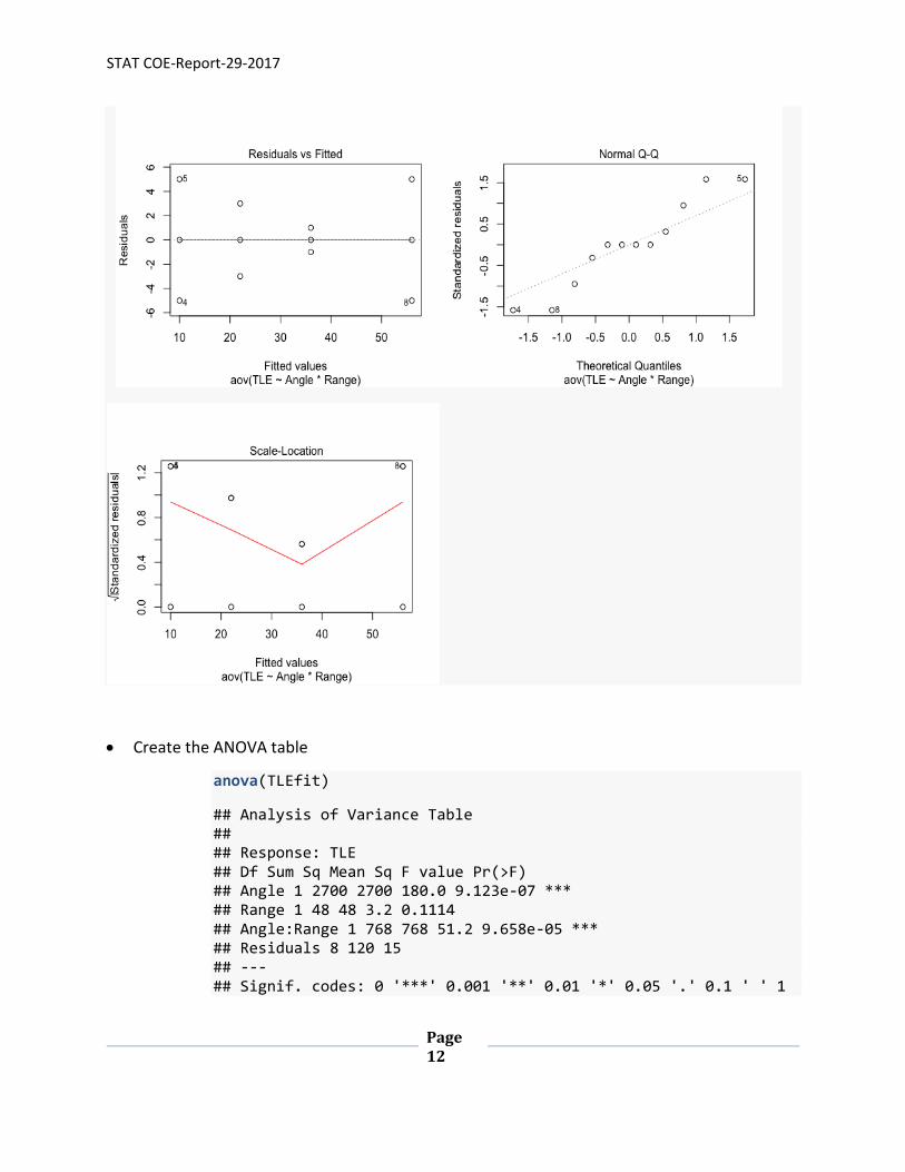
Check the assumptions

plot(TLEfit)


Page 12

Create the ANOVA table

anova(TLEfit)

## Analysis of Variance Table ## ## Response: TLE ## Df Sum Sq Mean Sq F value Pr(>F) ## Angle 1 2700 2700 180.0 9.123e-07 *** ## Range 1 48 48 3.2 0.1114 ## Angle:Range 1 768 768 51.2 9.658e-05 *** ## Residuals 8 120 15 ## --- ## Signif. codes: 0 '***' 0.001 '**' 0.01 '*' 0.05 '.' 0.1 ' ' 1


Page 13

We can note the p-values [Pr(>F) in R] to determine which factors are significant in the model. Both

Angle and Angle*Range, the two-factor interaction, are significant with small P-values, while Range is

not significant. However, Range should not be removed from the model since the higher order

interaction Angle*Range is significant.

Show the coefficients and the interaction plot

TLEfit$coefficients

## (Intercept) Angle Range Angle:Range ## 31 -15 2 -8

interaction.plot(Angle, Range, TLE)

From the ANOVA table, we would then conclude that our final model should be 𝑌𝑖𝑗𝑡 = 𝜇 + 𝛼𝑖 + 𝛽𝑗 +

(𝛼𝛽)𝑖𝑗 + 𝜖𝑖𝑗𝑡. The interaction plot is another way to show that keeping the interaction term is

necessary as the lines are not parallel. The coefficients allow us to fully construct the model, �̂� = 31 −

15(𝐴𝑛𝑔𝑙𝑒) + 2(𝑅𝑎𝑛𝑔𝑒) − 8(𝐴𝑛𝑔𝑙𝑒 ∗ 𝑅𝑎𝑛𝑔𝑒). Recall, these are in coded -1 and 1 units.


Page 14

JMP 1. Enter the data into JMP

2. Check that Angle and Range are nominal variables by left clicking the symbol next to the

variable.

3. Select “Analyze -> Fit model”

4. Enter TLE into the Y by selecting the variable and then clicking “Y”. Enter the full factorial of the

responses into construct model effects by highlighting Angle and Range, then selecting

“Macros” and selecting the full factorial option.


Page 15

5. Select “Run”

6. Observe the ANOVA, Parameter estimates, and effects test tabs for important p-values. The

ANOVA table p-value tells if there is a difference in means due to any factor. The other two tabs

further break it down to show which factor is causing the difference.

7. *Optional* If needed, remove any non-significant terms using the effect summary. Highlight the

term that needs to be removed and select “Remove” at the bottom of the window.


Page 16

*Remember, do not remove Range

because it is also included in the

higher order interaction of

Angle*Range.

8. Observe the Interaction plot. Select “red drop down arrow -> Factor profiling -> Interaction

plots”

Interaction Profiles

The conclusions we draw using JMP are the same as those from using R.

Conclusion ANOVA is a powerful tool used to determine which factors are significant in affecting the response. The

overall goal of ANOVA is to select a model that only contains significant terms. ANOVA can work for a

single factor or be extended to multiple factors. A number of hypotheses have been presented that can

be analyzed using ANOVA. Through the use of ANOVA, one can obtain a model that accurately

represents the data without including terms that do not.


Page 17

References Burke, Sarah. “The Model Building Process Part 1: Checking model Assumptions.” Scientific Test and

Analysis Techniques Center of Excellence (STAT COE), 12 Oct. 2017.

Dean, Angela & Voss, Daniel Design and Analysis of Experiments. New York: Springer Science + Business

Media Inc., 1999.

Montgomery, Douglas C. Design and Analysis of Experiments. 9th ed., John Wiley & Sons, Inc., 2017

Understanding Analysis of Variance

Documents

Transcript of Understanding Analysis of Variance