UNCLASSI(FIED

AD 403 813

DEFENSE DOCUMENTATION CENTERFOR

SCIENTIFIC AND TECHNICAL INFORMATION

CAMERON STATION. ALEXANDRIA. VRGINIA

UNCLASSIFIED

NOTICE: When goverment or other drawings, speec-fications or other data are used for any purposeother than in connection vith a definitely relatedgoverment procurement operation, the U. S.Goverment thereby incurs no responsibilityo nor anyobligation vhatsoever; and the fact that the Govern-ment may have formulated, furnished, or in any wysupplied the said drawings, specifications, or otherdata is not to be regarded by implication or other-wise as in any manner licensing the holder or anyother person or corporation, or conveying any rightsor permission to manufacture, use or sell anypatented invention that my in any Way be relatedthereto.

SAloR A. P*C''' AERONAUTICAL RESEARCH ASSOCIATES of PRINCETON, INC.

AFOSR TN 60-1227 CONTRACT AF 49(638)-255

(ARAP Report No. 50)

EXAMINATION OF THE SOLUTIONSOP THE NAVIER-STOKES EQUATIONS

FOR A CLASS OF THREE-DIMENSIONAL

VORTICESPart II: Velocity and Pressure

Distributions for Unsteady Motion

byColeman duP. Donaldson

and

Roger D. Sullivan

Prepared forAir Force Office of Scientific ResearchAir Research and Development Command

United States Air ForceWashington 25, D. C.

November 1962

Aeronautical Research Associates of Princeton, Inc.50 Washington Road, Princeton, New Jersey

17

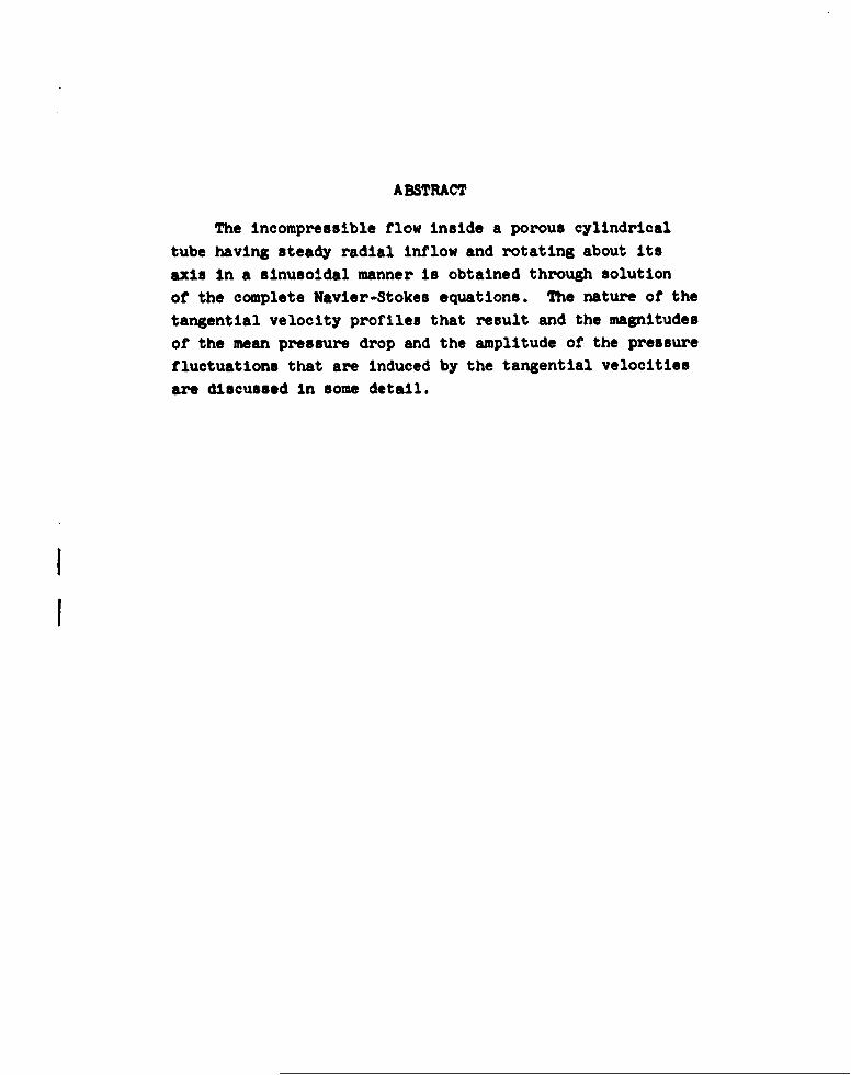
ABSTRACT

The Incompressible flow inside a porous cylindrical

tube having steady radial Inflow and rotating about its

axis In a sinusoidal manner is obtained through solution

of the complete Navier-Stokes equations. The nature of the

tangential velocity profiles that result and the magnitudes

of the mean pressure drop and the amplitude of the pressure

fluctuations that are Induced by the tangential velocities

are discussed in some detail.

I

TABLE OF CONTENTS

1. Introduction 1

2. Basic Equations 3

3. Velocity Distributions 6

4. Pressure Distributions 7

5. Discussion of Results 10

References

I1

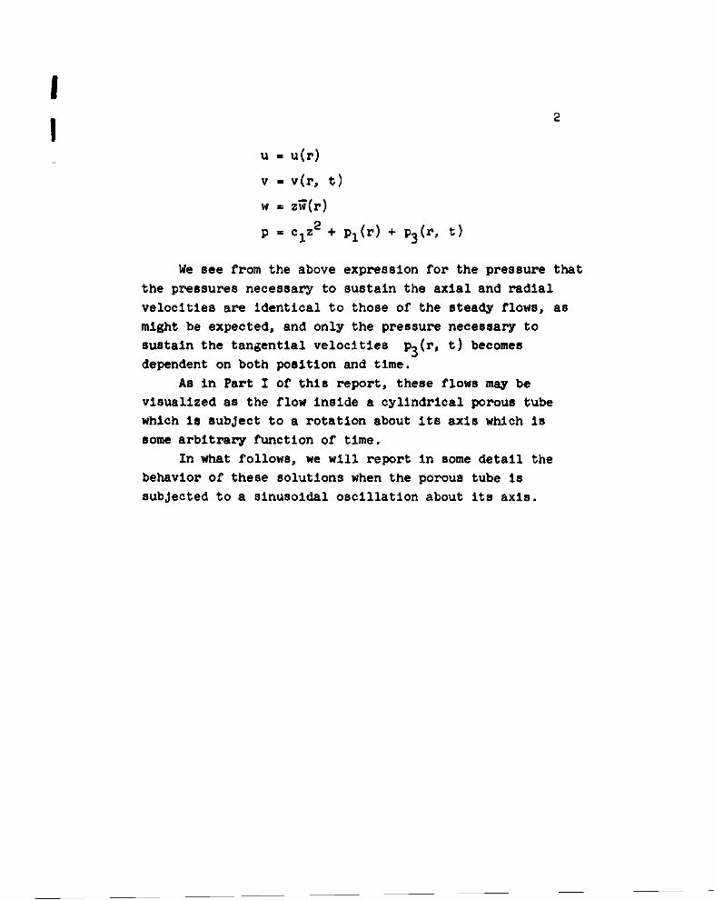
1. Introduction

In reference I (hereafter referred to as Part I)

we considered the behavior of a class of three-dimensional

steady solutions of the Navier-Stokes equations. The

flows considered were those such that, in a cylindrical

coordinate system (r, 0, z), the radial, tangential, and

axial velocity distributions were of the form

u - u(r)

v - v(r)

w - z9(r)

while the pressure distribution was of the form

p a c z 2 + pl(r) + P2 (r)

In the above expression for the pressure one mayIdentify the term clz2 with the pressure necessary

sustain the axial velocities, the term pl(r) with the

pressures necessary to sustain the radial motion, and the

term p2 (r) with the pressures necessary to sustain thetangential velocities.

This special class of steady solutions of the Navier-

Stokes equations is such that the equations for the radial

and axial components of velocity are decoupled from theequations governing the tangential velocity distribution

and the distribution of pressure. Because of this decoupling

of the equations, one finds that for very little additional

labor one can obtain the behavior of a simple class of

unsteady solutions of the Navier-Stokes equations; namely,

solutions of the form

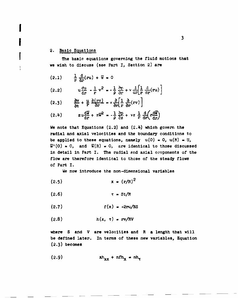
2

u - u(r)

v - v(r, t)

w = z;(r)

p I clz2 + p,(r) + p3 (r, t)

We see from the above expression for the pressure that

the pressures necessary to sustain the axial and radial

velocities are identical to those of the steady flows, as

might be expected, and only the pressure necessary to

sustain the tangential velocities P 3 (r, t) becomes

dependent on both position and time.

As in Part I of this report, these flows may be

visualized as the flow inside a cylindrical porous tube

which is subject to a rotation about its axis which Is

some arbitrary function of time.

In what follows, we will report in some detail thebehavior of these solutions when the porous tube issubjected to a sinusoidal oscillation about its axis.

I3

2. Basic Equations

The basic equations governing the fluid motions that

we wish to discuss (see Part I, Section 2) are

(2.1)r dr

dr r a 4r 7ru

(2.2) dr + -_ + v z d dQr\drj

We note that Equations (2.2) and (C.4) which govern the

radial and axial velocities and the boundary conditions to

be applied to these equations, namely u(O) - 0, u(R) - U,7'(0) = 0, and i(R) a 0, are identical to those discussed

in detail in Part I. The radial and axial components of the

flow are therefore identical to those of the steady flows

of Part I.

We now introduce the non-dimensional variables

(2.5) x _ (r/R) 2

(2.6) r= St/R

(2.7) f(x) - -2ru/RS

(2.8) h(x, r) - rv/RV

where S and V are velocities and R a length that willbe defined later. In terms of these new variables, Equation

(2.3) becomes

(2.9) xhxx + nfh, a nh

4

where the subscripts indicate differentiation with respectto the variables x and T and the parameter n - RS/4v

is a Reynolds number.

Now let R be the internal radius of a porous cylinderoscillating in such a manner that

(2.10) v(R, t) = V cos a•t

Applying this boundary condition to h(x, r) gives us

(2.11) h(l, T) = cos nr

where fn = Rc'/S. We also require that the tangentialvelocity vanish at r - 0, so that we have

(2.12) h(0, T) - 0

If we write

(2.13) h - R.P.{A(x)e"int} . x cos Qt + w. sn nt

where A(x) = X(x) + i4(x), then Equation (2.9) becomes

(2.14) xA" + nfA' = -inCA

The boundary conditions (2.11) and (2.12) are

(2.15) A(O) = 0 A(M) - 1

Let O(x) - a(x) + ip(x) be a solution of Equation (2.14)when 0(0) - 0 and 0'(0) 1 1. Then the solution we

require is

A(x) O- 0(l)

5

or writing 0(l) - al + i1 we have

(2.16) - I

(2.17) X(x) = 1 1a1 1

where a(x) and O(x) are solutions of

(2.18) xa" + nfa' -nfl

subject to c(O) = 0 and a:(O) = 1 and

(2.19) xO" + nfP' - -nOa

subject to P(O) 0 and 0'(O) = 0.

In order to ure the results presented in this report

it is necessary to specify the characteristic velocity S.

As is discussed in Part I (p. 38), the characteristic

velocity S is the numerical value of the axial velocity

at r a 0 and z = R. The exact value of S in relation

to the radial inflow or outflow at r = R is obtained from

the steady solution for the radial and axial velocities.

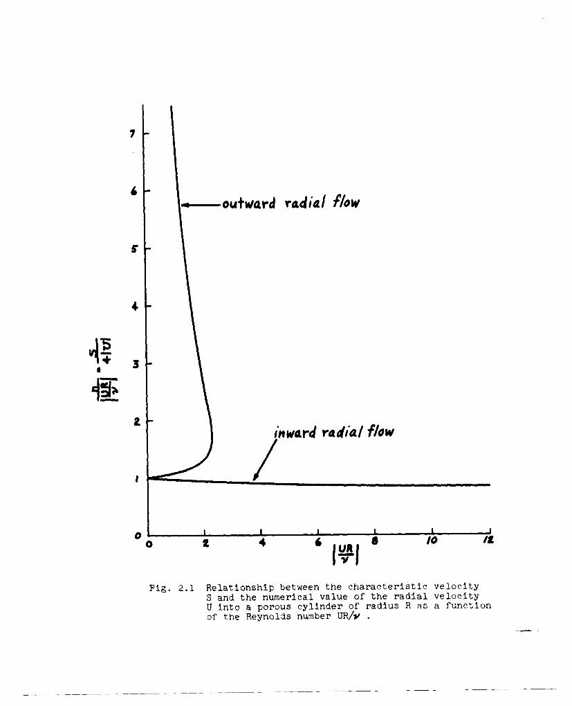
Figure 2.1 is a plot of the ratio of n/IUR/vJ = S/4IUI

as a function of IUR/vi for the simple families of one-

celled flows obtained from the studies reported in Part I.

As is indicated in this figure, one-celled flows under

conditions of outward radial flow exist for only a limited

range of radial Reynolds number (for a more extended dis-

cussion see Part I). For this reason, we shall limit the

computations and discussion to the case of radial inflows.

7

do- outward radial flow

4-

3

Fig. 2.1 Relationship between the characteristic velocityS and the numerical value of the radial velocityU into a porous cylinder of radius R as a function

of the Reynolds number UR/V.

I6

3. Velocity Distributions

An analog computing machine was used to solve

Equations (2.18) and (2.19) and thus determine the functions

X(x) and i±(x) which represent the tangential velocity

distribution, for a range of both the frequency parameter

n and the Reynolds number n. In making these computation~s

the radial velocity function f(x) was generated by

simultaneous solution of the appropriate equation for f

subject to the proper boundary conditions (Equations

(2.2.6), (2.2.8), (2.2.9), and (2.2.10) of Part I). Typicaltangential velocity profiles at an instant in time and

envelopes of the velocity profiles for all times are shown

in Figures 3.1, 3.2, 3.3, and 3.4 with the Reynolds number

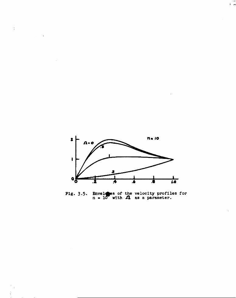
n as a parameter for four values of the frequency parameter(0 = 0, 0.3, 1.0, and 3.0 respectively). In Figure 3.5

the envelopes of the velocity profiles are shown for the

particular Rey'nolds number n - 10 with 0 as a parameter.

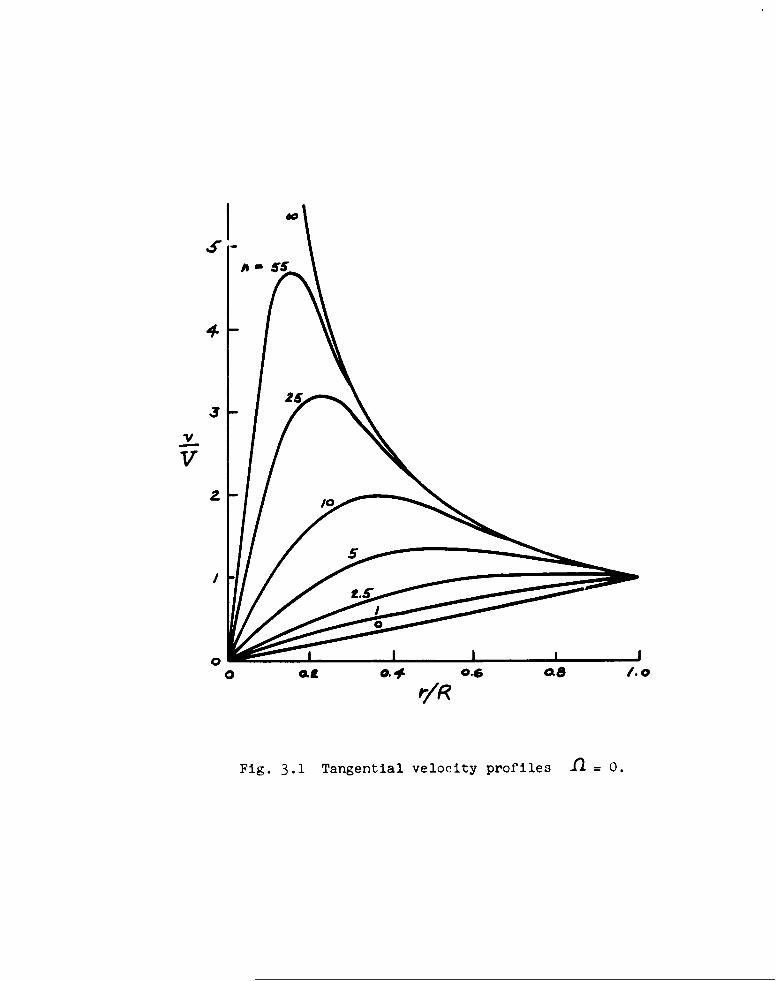
A" 55

V

0 f o.@o. 08 /.o

ivR

Fig. 3.1 Tangential velocity profiles 0 .

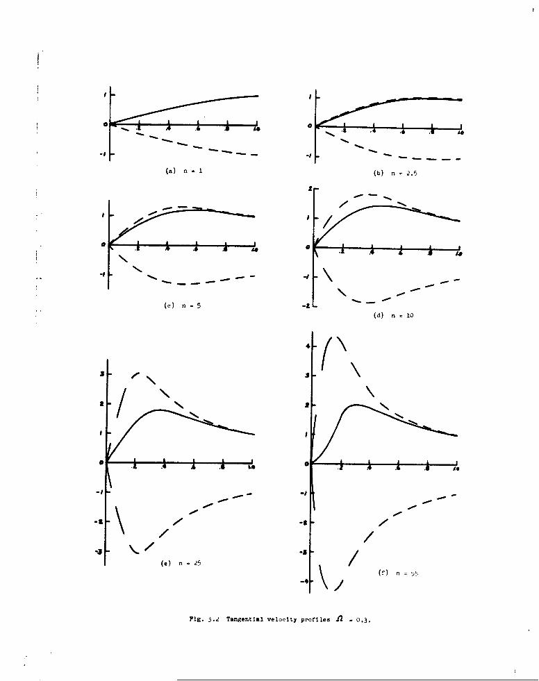
(a) nl- (b) n 2.

0*

(c') n=5-

(d) n =10

I4

(e) n

Fig. 3.,! Tangential velocity profiles nt o,03.

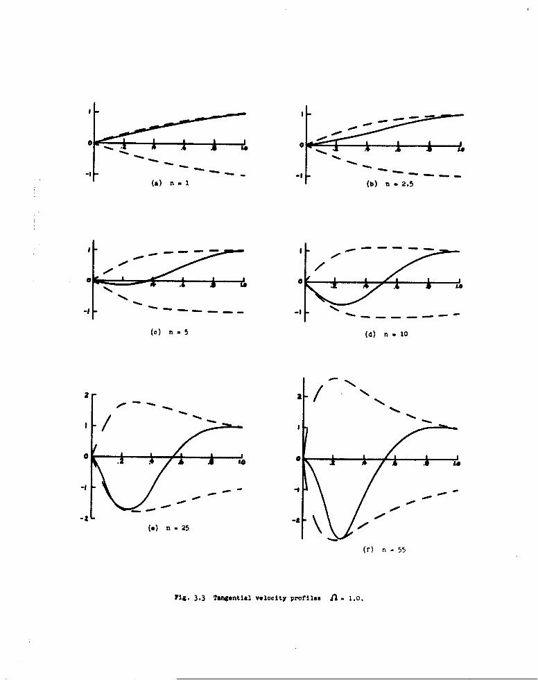
(a) n- (b) n -2.5

(C) n=5 Cd) n 10

-0 N

00

(s) n -25 0

C)n - 55

Fig. 3.3 Tangential velocity profiles 1 .0.

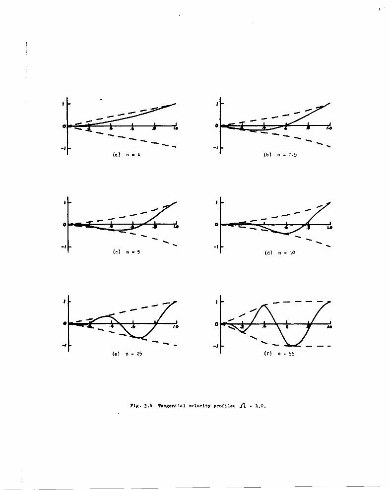
0~ ~~~ ~ ~ ~ ... ...................t...... .... 11

(a) n. (b) n- 2.5

0

- L-O I•

(c) n- 5 (d) n = 10

.0

(e) n- 25 (f) n 55

Fig. 3.4 Tangential velocity profiles .11 - 3.0.

"" a IO

0 .4. .6 .4oL

Fig. 3.5. EnvelQes of the velocity profiles forn - lawith A as a parameter.

7

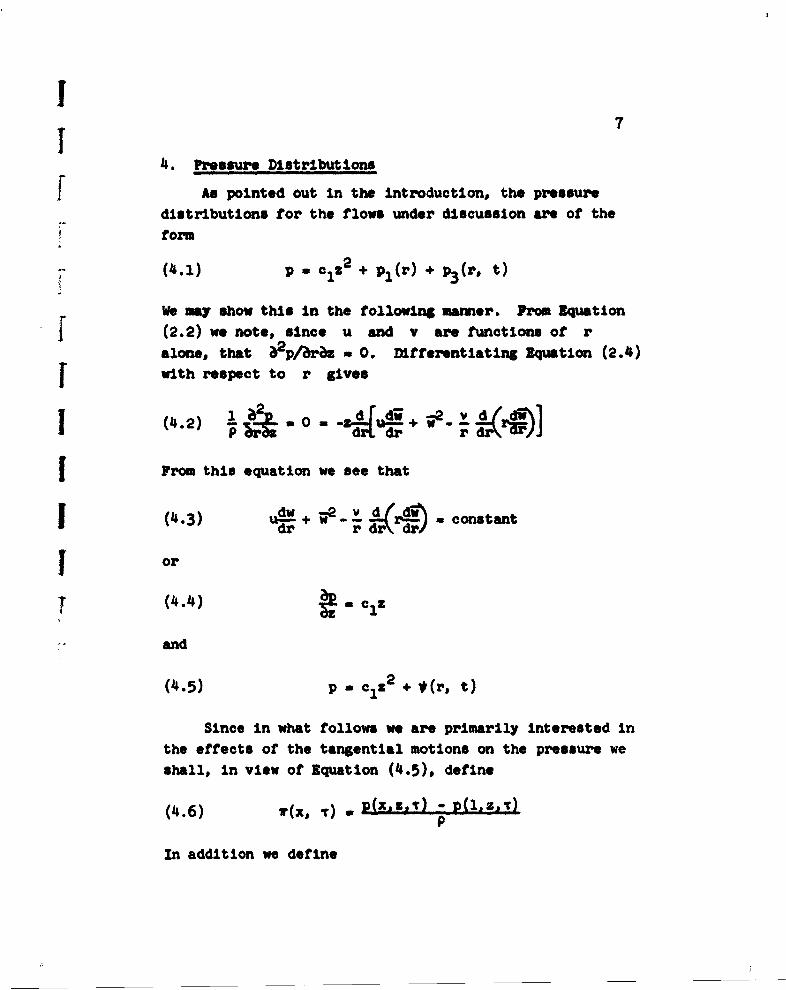
4. Pressure Distributions

As pointed out in the introduction, the pressure

distributions for the flows under discussion ame of the7"i form

+-- ((4.1) p - clZ2 + p,(r) + p3 (r, t)

We my show this In the following manner. From Equation

(2.2) we note, since u and v are functions of ralone, that a•p/r&-z . 0. Differentiating Equation (2.4)

f with respect to r gives

(,4.2) b2--+ ; _.-P -' r I

From this equation we see thatdw -2 consdw-

(4.3) u- -=con. sdtantIF+w r i d

or

(14.14) C " 1c

and

(4.5) p c z2 + *(r, t)

Since in what follows we are primarily interested inthe effects of the tangential motions on the pressure weshall, In view of Equation (4.5), define

(4.6) jr(x, 1) -(x,,) 0(1.z.r)

"n ap

In addition we define

!8

, (4.8) 712(x) . d

(41.9) ,r22 W - ,f -ft

-. (1(.10) V 3 (x) -- x[r2(,)

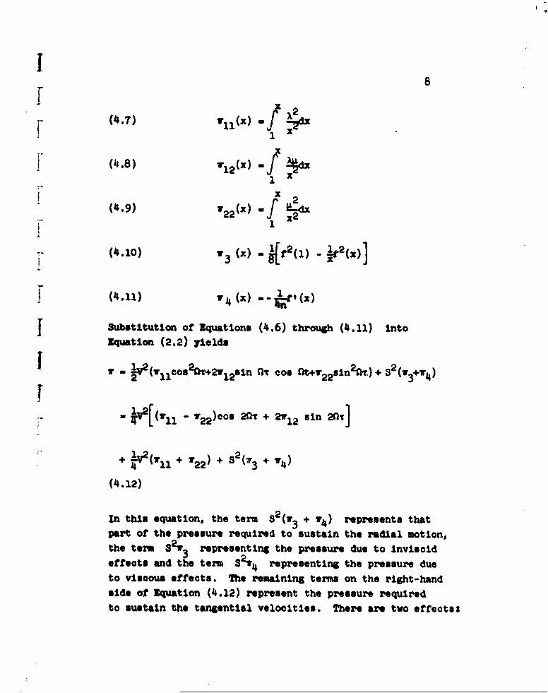
I Substitution of Equations (4.6) through (4.11) intoEquation (2.2) yields

S• - y 2 (. 11os2fr+2w , sin Ch 005 fot+7 22 sIl 2nT. )+ S2 (, 3+74)

. 2[c,,, -. 22)cos 2fl + 2 si,.,n 20T]

+ •-P(w + Tr22) + S2(T3 + 74)

(41.12)

In this equation, the term 82(T3 + w4) represents thatpart of the pressure required to sustain the radial motion,the term 832w3 representing the pressure due to Inviseldeffects and the term 32r4 representing the pressure dueto viscous effects. The remaining terms on the right-handside of Equation (4.12) represent the pressure requiredto sustain the tangential velocities. There are two effectest

9

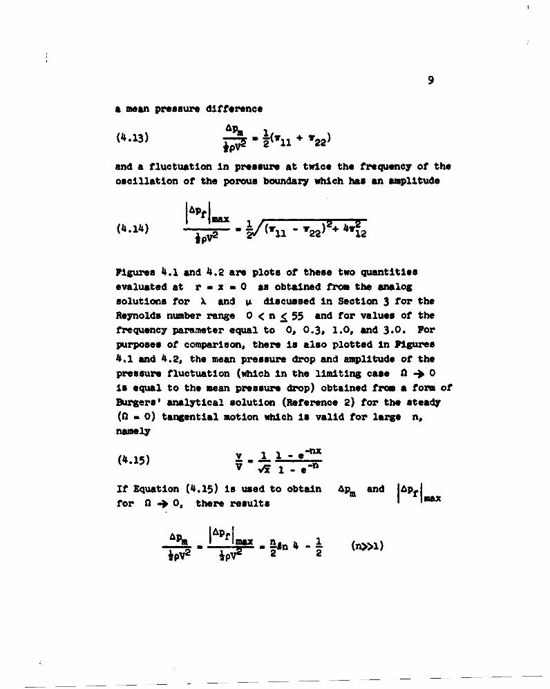
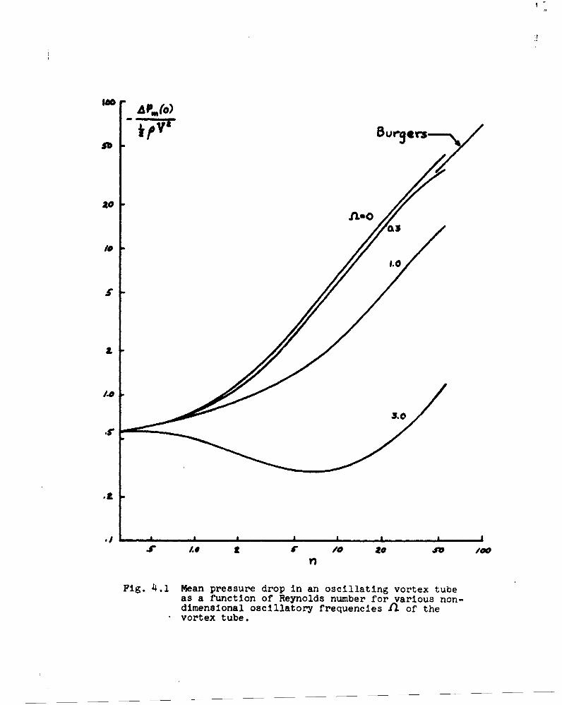
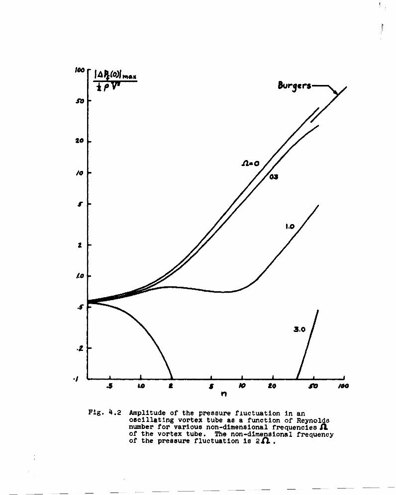
a mean pressure difference

(4-.13) A+

and a fluctuation In pressure at twice the frequency of theoscillation of the porous boundary which has an amplitude

jpV2 - (rll " 22)+ 41

Figures 4.1 and 4.2 are plots of these two quantities

evaluated at r a x - 0 as obtained from the analog

solutions for X and KI discussed In Section 3 for theReynolds number range 0 < n 1 55 and for values of the

frequency parameter equal to 0, 0.3, 1.0, and 3.0. Forpurposes of comparison, there is also plotted in Figures4.1 and 4.2, the mean pressure drop and amplitude of the

pressure fluctuation (which In the limiting case -+ 0Is equal to the mean pressure drop) obtained from a form of

Burgers' analytical solution (Reference 2) for the steady(n - 0) tanWential motion which is valid for large n,

namely

(4.15) v- , -nV VT 1 *-

If Equation (4.15) Is used to obtain Ap, and I-apt1mfor n 4 0, there results

- ,•P 4 1 (n))l)JpV2 Jp2 2 2

Bur~ers~~

50

ao IL&-O

I,

I.e

...

.2

5. g 5" /0 O00 S10

Fig. 4.1 Mean pressure drop in an oscillating vortex tubeas a function of Reynolds number for various non-dimensional oscillatory frequencies il of thevortex tube.

jtP " B•rSers

to

.a.0/00

3.0

.O LO A V *0 /60

Fig. 4.2 Amplitude of the pressure fluctuation in anoscillating vortex tube as a function of Reynoldsnumber for various non-dimensional frequencies Tof the vortex tube. The non-dimensional frequencyof the pressure fluctuation is 211.

10

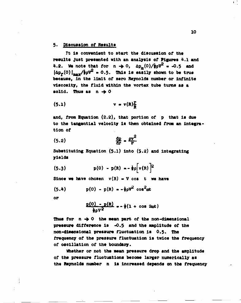
5. Discussion of Results

Tt In convenient to start the discussion of the

results Just presented with an analysis of Figures 4.1 and

14.2. We note that for n 40, &p,(O)/ipV2 , _0.5 and

IApt(O)Ie/ApV". -0.5. "is is easily shown to be truebecause, in the limit of zero Reynolds number or infinite

viscosity, the fluid within the vortex tube turns as asolid. Thus as n 4 0

(5.1) v -. )

and, from Equation (2.2), that portion of p that is dueto the tangential velocity Is then obtained from an Integra-

tion of

2(52)dr r

Substituting Equation (5.1) Into (5.2) and integratingyields

(5.3) p(o) - p(R) a- p[v(R) ]2

Since we have chosen v(R) - V cos t we have

(5.4) p(O) - p(R) -- _ pV2 cos 20t

or

P(O) -D(R m--(l + coo 2wt)

Thus for n 4 0 the mean part of the non-dimensional

pressure difference is -0.5 and the amplitude of the

non-d•mensional pressure fluctuation Is 0.5. Thefrequency of the pressure fluctuation Is twice the frequency

of oscillation of the boundary.

Whether or not the mean pressure drop and the amplitude

of the pressure fluctuations become larger numerically as

the Reynolds number n is Increased depends on the frequency

11

parameter 0. For frequency parameters smaller than unity,the general trend is for the pressure difference and ampli-tude to increase numerically as n Increases. As 11

becomes larger than unity, the tendency is for the mean

pressure differences and amplitudes to at first decreasenumerically as n becomes larger than unity and thenfinally increase at some Reynolds number. The Reynolds

number at which the pressure fluctuations start to increase

is a function of 0. The larger 11 becomes, the larger isthe range of n above unity for which the mean pressuredifferences and the amplitudes of the pressure fluctuations

du& to the oscillating boundary are of small magnitude.Eventually, for an incompressible fluid, all curves such

as those shown In Figures 4.1 and 4.2 must turn upwardsbecause, given any finite frequency no matter how high, onecan always choose a Reynolds number high enough so that the

shears developed between successive maxima of the velocity

distribution curves become negligible. When this condition

exists, the fluid introduced through the porous boundary

is able to maintain to some degree its initial angularmomentum with the result that high tangential velocities are

carried toward the axis. In an incompressible medium these

high tangential velocities cause pressure fluctuations

that are transmitted instantaneously to the boundaries ofthe flow. It appears from what has been said above andfrom the behavior of the solutions which have been obtained,

that for all finite frequencies the mean pressure difference

and the amplitude of the pressure fluctuations becomeproportional to n as n -a u, as has been discussed for

the case 0 a 0 in Section 4.The reason for the initial drop In the numerical

values of &Pm(O) and IApf(O)Imax as n increases for

frequency parameters greater the unity can best be explained

as follows. At low Reynolds numbers (n << 1), the viscosity

I12I

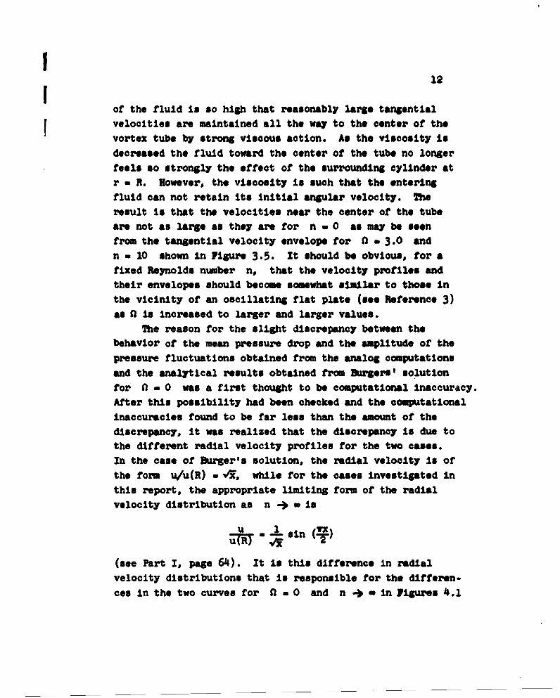
of the fluid is so high that reasonably large tangentialf• velocities are maintained all the way to the center of the

vortex tube by strong viscous action. As the viscosity isdecreased the fluid toward the center of the tube no longerfeels so strongly the effect of the surrounding cylinder atr - R. However, the viscosity is such that the enteringfluid can not retain Its Initial angular velocity. Theresult is that the velocities near the center of the tubeare not as large as they are for n - 0 as may be seenfrom the tangential velocity envelope for 0 a 3.0 andn - 10 shown in Figure 3.5. It should be obvious, for afixed Reynolds number n, that the velocity profiles andtheir envelopes should become somewhat similar to those Inthe vicinity of an oscillating flat plate (see Reference 3)

as ins increased to larger and larger values.The reason for the slight discrepancy between the

behavior of the mean pressure drop and the amplitude of thepressure fluctuations obtained from the analog computationsand the analytical results obtained from Burgers' solutionfor n - 0 was a first thought to be computational Inaccuracy.After this possibility had been checked and the computationalInaccuracies found to be far less than the amount of thediscrepancy, it was realized that the discrepancy is due tothe different radial velocity profiles for the two cases.In the case of burger's solution, the radial velocity Is ofthe form u/u(R) - v, while for the cases Investigated Inthis report, the appropriate limiting form of the radialvelocity distribution as n -I * is

U-7 ~sin (wx

(see Part I, page 64). It Is this difference in radialvelocity distributions that is responsible for the diffeoren-ces In the two curves for n m 0 and n - a in Figures 4.1

13

and 4.2.It is interesting to note that for the particular

case of flows for which the radial velocity at r a R isproportional to the tangential velocity at r - R, thepressure fluctuations in the flow will vary as V3 forhigh enough Reynolds number since, in this case, theReynolds number n is proportional to V and, for highenough Reynolds number for a fixed frequency,1Apf(0)1mX/*pV2 becomes proportional to n.

1. Donaldsont Coleman duP. and Sullivan, Updozo D.

Examination of the Solutions of the NavL or-Stokes

Equations for a Class ot Three-DiaenosiCAl Vorticel,

Part I: Velocity Distributions for Stlb-4 Notion.

APOSR TN 60-1227, October 1960.

2. Burg-ers, J. N. A VIthematical Model iIIIustrating the

Theory of Turbulence. Adv. in Appi. NW.e* Vol. I,

PP. 197-199. Academic Press, 1948.

3. Schlichtingr N. Boundary Layer Theory, NcOe~r-Hll,

pp. 75-76, (1960).