UNCLASSI FIEDI, A417202/

DlEFENSE DOCUMENTATION CENTERFOR

SCIENTIFIC AND TECHNICAL INFORMATION

CAMERON STATION, ALEXANDRIA, VIRGINIA

U LFI

, UNCLASSIFIED

NOTICE: Ifhen govermnt or other drawings, speci-fications or other data are used for any purposeother than in connection with a definitely relatedgovernment procurement operation, the U. S.Government thereby incurs no responsibility, nor amyobligation vhatsoever; and the fact that the Govern-ment may have formulated, furnished, or in any vaysupplied the said drawings, specifications, or otherdata is not to be regarded by Implication or other-wise as in any -anner licensing the holder or anyother person or corporation, or conveying any rightsor permission to nuzmfacture, us. or s12. anypatented invetion that may :In ay vay be WeAtedthereto.

OPERATIONAL EVALUATION OF AIRPORT

RUNWAY DESIGN AND CAPACITY1 (A Study of Methods and Techniques)

0

i-CD,

REPORT NO. 7601-6

Contract FAA/BRD-136

January 1963

Prepared for

Federal Aviation AgencySystems Research Development Service

Research DivisionProject No. 412-7-IR

This report Is been approved for general distribution.

AIRBORNE INSTRUMENTS LABORATORY 4 %:3A DIVISION OF CUTLER-HAMMERINC. SE Z4Deer Park, Long Island, New York lboq4 G U a I-

99

OPERATIONAL EVALUATION OF AIRPORT

RUNWAY DESIGN AND CAPACITY

(A Study of Methods and Techniques)

By

E. N. Hooton, H. P. Galliher, M. A. Warskow,

and K. G. Grossman

REPORT NO. 7601-6

Contract FAA/BRD-136

January 1963

Prepared for

Federal Aviation AgencySystems Research Development Service

Research DivisionProject No. 412-7-1R

This report has been prepared by Airborne Instru-ments Laboratory for the Systems Research andDevelopment Service, Federal Aviation Agency,under Contract FAA/BRD-136. The contents of thisreport reflect the views of the contractor, who isresponsible for the facts and the accuracy of thedata presented herein, and do not necessarilyreflect the official views or policy of the FAA.

AIRBORNE INSTRUMENTS LABORATORYA DIVISION OF CUTLER-HAMMER, INC.

Deer Park, Long Island, New York

ACKNOWLEDGMENTS

We wish to thank the many people who gave us their

assistance and cooperation during this study, particularly

individuals in the Federal Aviation Agency Airports Service,

Systems Research and Development Service, and air traffic con-

irollers at Washington National, Chicago O'Hare, Denver, Idle-

wild, and Los Angeles International airports. Within the

Systems Research and Development Division, Messrs. E. Dowe

and 0. Shapiro were particularly helpful with their comments

and review of the project work and report. We also wish to

acknowledge the contributions of the following people at

Airborne Instruments Laboratory: I. D. Kaskel, C. Spruck,

K. Andrews, M. E. Demarco, and F. B. Pogust.

Ii

FOREWORD

This report is one of a series of three volumes

containing the results of a study program on airport runway

and terminal design. The program is a continuation of previ-

ous work published under the title, "Airport Runway and Taxi-

way Design". The three volumes describing the new work con-

sist of this volume, a handbook entitled "Airport Capacity, 1"

and a previous volume entitled "Airport Terminal Plan Study."

Additional practical applications of the techniques described

in this report can also be found in "Airport Facilities for

General Aviation," prepared by Airborne Instruments Laboratory

under Contract FAA/BRD-403.

ABSTRACT

This report describes a continuation of research

into the application of mathematical techniques to the evalu-

ation of practical airport capacity and delays. Since the

primary task was to develop a handbook for determining airport

capacity and delays by the engineer in the field, the main

effort was concentrated on developing existing mathematical

models for universal application. Therefore, this report

contains the background material relevant to the handbook,

describes the mathematical models used, and discusses the

preparation of their respective inputs. These inputs vary

with runway configuration, runway use, aircraft population,

and operating rules (VFR or IFR). The airport surveys that

were analyzed to provide input values and operating param-

eters are also described. An IBM 7090 Fortran program

was written to automatically compute the inputs and model

outputs in the form of delays versus operating rates and

capacities of airport runway configurations. The use and

application of this program is described.

V

TABLE OF CONTENTS

Page

Acknowledgments i

Foreword iii

Abstract vGlossary xiii

I. Introduction 1-1

A. General 1-1

B. Advanced Model Applications 1-2

II. Refinements of Steady-State Mathematical 2-1Models for VFR Operations

A. Variability in Service Times 2-2

B. Arrival/Landing Process 2-4

C. Relationship of Arrival Spacing 2-7to Departures

D. Dual Arrival Feed 2-12

III. Refinements of Steady-State Mathematical 3-1

Models for IFR Operations

A. Single Runway 3-2

B. Intersecting Runways 3-5C. Close Parallel Runways 3-7D. Arrival Process 3-9

IV. Airport Surveys and Performance Data 4-1

A. Method of Data Taking 4-1

B. Data Reduction 4-3C. Formation of Inputs 4-5

D. Model Testing 4-19

V. Description of Mathematical Models 5-1

A. General 5-1

B. Formulation of Delay 5-4

vii

TABLE OF CONTENTS (cont)

Page

VI. Preparation of Airport Capacity Handbook 6-1A. General 6-1

B. Handbook Description 6-6

VII. References 7-i

VIII. Conclusions 8-1

IX. Recommendations 9-1

Appendix A--Time-Dependent Nonstationary A-1Runway Model

Appendix B--Determination of Delay Using B-1Steady-State Models in Non-stationary Situations

Appendix C--Effects of Airport Altitude C-1on Runway Capacity

Appendix D.--Analysis of Aircraft Speeds D-1on Approach

Appendix E--Mathematical Description of E-1Multi-Server Queuing ModelUsed to Compute Gate Delay

Appendix F--Runway/Taxiway Crossing F-1

viii

LIST OF ILLUSTRATIONS

Figure

2-1 Spacing Factors (Inputs) for Pre-emptive SpacedArrivals Model (SAM) for Single Runway

2-2 Spacing Between SuccessiJve Departures on Two Inter-secting Runways

2-3 Basic Arrival Feeds to Dual Runways

3-1 Departure/Arrival Service Time in IFR (Effect ofIntersecting Runways)

3-2 Departure/Departure Service Time in IFR (Effectof Intersecting Runways and Initial Departure Route)

4-1 Airport Survey Recording Technique

4-2 Example of Airport Data Plot

4-3 Distance vs Time for Takeoff, Class A

4-4 Distance vs Time for Takeoff, Class B4-5 Distance vs Time for Takeoff, Class C

4-6 Distance vs Time for Takeoff, Class D

4-7 Distance vs Time for Takeoff, Class E

4-8 Distance vs Time for Landing, Class A

4-9 Distance vs Time for Landing, Class B

4-10 Distance vs Time for Landing, Class C

4-10 Distance vs Time for Landing, Class D

4-12 Distance vs Time for Landing, Class E

4-13 Runway Rating Curves

4-14 Sample Data from Survey, Interval A (IFR)

6-1 Intersecting Runway with Close Intersections

6-2 Simplified Flow Diagram of Airport Capacity Program(IBM 7090 Computer)

6-3 Example of Computer Output

B-1 Comparison of Steady-State Delay with Time-DependentDelay

B-2 Time Needed to Reach Steady-State Delay

C-1 Intervals of T Measured at Denver

C-2 Intervals of A Measured at Denver

D-1 Aircraft Approach Speeds from 10 to 5 Miles

ix

LIST OF TABLES

Table Page

4-i Aircraft by Type and Class 4-23

4-11 T, Average Minimum Spacing Between Suces- 4-25sive Departures on Same Runway (VFR) "

4-111 Time from "Clear to Takeoff" to "Start 4-28Roll" for Departures

4-IV T, Average Minimum Spacing Between Sucees- 4-29sive Departures on Same Runway.and SameDeparture Rout.e (IFR)

4-V T, Average Minimum Spacing Between.Succee- 4-32sive Departures on Same Runway but -on Dif-ferent Departure Routes (IFR).

4-VI Absolute Mini-mum Values .of F for Same Run- 4-35way (VFR)

4-VIi Ave'age Minimum Values of F for Same. Runway 4-36(IFR)

4-ViII Average Time from Over-Threshold to Runway, 4-37Touchdown for Arrivals in VFR (Equals Valueof R for Open V Runways)

4-IX Average Time from Over-Threshold to Runway "4-38'Touchdown for Arrivals in IFR (Equals Valueof R for Open V and Close Parallel Runways)

4-x A, Average Minimum Spacing Between Succes-• 4 39.sive Arrivals (VFR)

4-xI A, Average Minimum Spacing Between Succes-" 4-42".sive Arrivals (IFR)

4-xii Model Testing Actual vs Computed Delays - 4-45Final Phase Testing

4-Xiii First Phase Testing Reported in reference 1' 4.-46

6-I T, Average Minimum Interval Between Succes- 6-19sive Departures on Same Runway (IFR Estimatefor 1970)

6-II F, Average Minimum Interval Required for 6-20* Departure Release in Front of an IncomingArrival.(IFR Estimate for 1970)

6.111 A, Average Minimum Interval Between Succes- 6-21sive Arrivals on Same Runway (IFR Estimatefor .1970)

xi

GLOSSARY

The average value (first moment) is indicated by a

small letter with subscript. For example, a1 is the first

moment of A,, and a2 is the second moment.

A Average minimum inter-arrival spacing

B Minimum arrival service time, B = R + C

C Average landing commitment interval

CL Commitment to land point

CT Cleared to takeoff

D Inter-departure time for departures

F Average minimum time required to release departurefor takeoff in front of an incoming arrival

FIM First-come, first-served model

FR CT(n-I) + J(n)

G Gap in inter-arrival spacing, G = L - B

H Interval that starts at end of K

IFR Instrument flight rules

J J=H+K

K Interval that starts when n-l departure takes off

L Inter-arrival time for arrivals

XL Arrival rate in landings per hour

XS Arrival rate plus departure rate

%T Departure rate in takeoffs per hour

OR Off runway

OT Over threshold

PAM Pre-emptive Poisson arrivals model

R Average runway occupancy for arrivals from "over*threshold" to "off runway"

xiii

I. INTRODUCTION

A. GENERAL

A comprehensive mathematical analysis of airport

runway and taxiway design has been carried out by Airborne

Instruments Laboratory (AIL) under the direction of the

Research Division, Systems Research and Development Service,

Federal Aviation Agency. This work has been reported upon

previously (reference 1) at a time when the formulation of

three basic mathematical models was completed. Since that

time, the effort has been devoted to the creation of infor-

mation that would be of more direct use to the airport engi-

neer in the field. This has necessitated a very close study

of IFR operations and various airport runway configurations.

The results of this current effort are incorporated

in three volumes: the present volume, an Airport Terminal

Plan Study, and an Airport Capacity Handbook. The separate

volumes are intended to simplify the use of the information

that has resulted from the rather diverse efforts that have

gone into the project. It is the purpose of this volume to

sum up the theoretical work in a form that will be of inter-

est to those working in the fields of research and develop-

ment. The mathematical formulations, theoretical and prac-

tical investigations, and certain peripheral studies that

have been included under the same contractual effort also

will be treated. This volume explains and supports the Airport

Capacity Handbook, which is concerned completely with the appli-

cation of the models. The Airport Terminal Plan Study (ref-

erence 2), which was prepared by Porter and O'Brien in cooper-

ation with AIL, covers the subject of the terminal building

and its supporting systems such as baggage handling and fuel-

1-1

ing. The mathematical approach to the probability of gate

occupancy (used in reference 2) is presented in this volume

as an Appendix.

B. ADVANCED MODEL APPLICATIONS

Since the publication of the last report, the work

on the runway mathematical models has continued with several

objectives. To provide a comprehensive handbook for deter-

mining airport capacity, it was necessary to extend the work

previously reported upon into several applications which are

more complex than those previously investigated. The first

of these were intersecting runways with mixed landings and

takeoffs on all runways in VFR. Such configurations consist

of two distinct types: (1) intersection occurring within the

lengths of each runway, and (2) intersections beyond the

runway lengths (open V with operations toward the apex).

Second, we had to perform a complete analysis of IFR oper-

ations, including the following: (1) single runways with

either mixed operations, landings only, or takeoffs only;

(2) intersecting and open V runways as in item 1; and (3)

additional analysis of close parallel runways where the sep-

aration between runways is less than 5000 feet. Techniques

for handling all of these situations have now been developed.

In accomplishing this new work, several simplifi-

cations and refinements in the basic models were found to be

possible. In addition, the entire symbology, which had proven

somewhat confusing in the earlier work, was simplified .and

clarified. The result of all of these improvements has made

the previous volume (reference 1) obsolete in many respects.

Therefore, a complete explanation of the models, their devel-

opment, and application will be presented in this report. It

should be stressed that this report provides the mathematical

and practical groundwork on which the Airport Capacity Hand-

1-2

book was based. Therefore, many of the actual conclusions

reached during this work will appear in the Airport Capacity

Handbook.

In addition to the basic work of developing the

models so that they would meet the Handbook requirements,

sever, ohlerperihera sudl±s were~ perfre and CLhes

are reported upon in this volume as Appendices A through E.

They include:

Time-Dependent Non-Stationary. Runway Model.Determination of Delay Using Steady-State Models inNon-Stationary Situations.

Effects .of Airport Altitude on Runway Capacity.

Analysis' of Aircraft Speeds on Approach.

Mathematical Description of Multi--Server QueuingModel Used for Computation -of Gate Delay.

Runway/yaxiway Crossings'.

1-3

II. REFINEMENTS OF STEADY-STATE MATHEMATICALMODELS FOR VFR OPERATIONS

Three mathematical models were described in the last

report.

1. First-Come,'First-Served Model (FIM),

2. Pre-emptive Spaced Arrivals Model (SAM),

3. Pre-emptive Poisson Arrivals Model (PAM).

The work previously described established that with

suitable inputs the three mathematical models provided a basis

for evaluating aircraft delay versus operating rate for single

runways and runway/taxiway crossings.

In this new work it was desired to extend this type

of analysis (that is, the practical application of mathemat-

ical techniques) to the following situations:

.1. ..Intersecting runways in VFR,

2. Dual arrival feed in VFR to multiplerunways,

3. IFR operations for all runway configura-tions.

This section is intended to give the reader a non-

""mathematical description of the work that was carried out to

meet these objectives. Therefore, it is presented in the

form'of a historical narrative since this method best describes

the logic that was used to solve the problems.

it was first established that the original SAM was,

the most effective model, but that certain rules of procedure

concerning the formation of the inputs for single-runway

operations could be simplified. These were:

2-1

1. The variability in service times.

2. The landing process and its effect ondeparture delay.

In analyzing these two aspects of SAM as applied toa single runway, it readily became apparent that the model

was also suitable for intersecting runways, and that the

effects of a dual arrival feed were quite simple to analyze.

A. VARIABILITY IN SERVICE TIMES

The SAM inputs were originally as follows:

1. Takeoff/takeoff interval ($2)y

2. Takeoff/landing interval (Sll),

3. Landing/landing interval (OT/OT),

4. Variability of item 3 expressed as aK (Erlang) factor,

5. Runway occupancy for landings (R1),

6. Runway commitment interval for landings[C1 = (oT-OT) - RIJ,

7. Landing and takeoff rates (X1 and X2 ).

Thus, the only variability from average values of

service times accounted for in the model was that for the

landing-to-landing interval. However, from the airport

observations taken up to that time, it was known that both

S2 and SI1 were extremely variable. For this reason, it wasfelt that these variabilities should be accounted for in SAM

to make the model truly representative of airport operations.

Therefore, SAM was initially modified to include the varia-

bility of S2 . This was done by introducing $22, which was

the second moment of S2 o

In the previous report the validity of SAM was

originally checked by comparing actual delays measured at

airports against computed delays (derived at identical move-

ment rates) from SAM. This technique was now applied to the

2-2

modified SAM model. The result was that, with variability

of S2 included, the computed delays were now far in excess

of the actual measured delays.

After some thought and a re-examination of the

airport data taken during the surveys, it became apparent

that the variability in service times of the various param-

eters was somewhat complex in their relationships to the

average service times. This is best illustrated by consider-

ing a typical airport operation of a single runway used by

arrivals and departures.

Two arrivals are approaching to land on the runway,

one spaced behind the other. Departures are being held await-

ing takeoff clearance since the local controller has decided.

that there is insufficient time before the first arrival to

release any departures.

The first arrival lands and rolls down the runway.

At this point the controller estimates that there is a suf-

ficient time interval before the next arrival to release at

least one and possibly two departures.

If this time interval, or arrival gap, is somewhat

short, the controller will request the first departure to

expedite his takeoff.. If a second departure is allowed to

go after the first, the second departure will also be required

to expedite the takeoff.

Thus, where the inter-arrival gaps are short, but

sufficiently long to permit departures, the-corresponding

departure service times can also be expected to be short.

In actual operations, there is a very strong relationship

between the variability of the inter-arrival gaps and the

departure service times..

Additional analysis and testing of the model against

actual data revealed that excellent agreement was obtained

2-3

between observed delay and computed delay if the average

values of the service times for departures were used.

B. ARRIVAL/LANDING PROCESS

The conclusions reached concerning the mean service

times-were applied to arrivals. In the then existing model,

the variability in the landing process was described as the

K (Erlang) factor, being a function of the standard deviation

of the average minimal arrival separation times at the runway

threshold.

It was decided to eliminate this particular input

from..the model and, at the same time, improve some of the

concepts of theoriginal model. These latter changes are best

detailed by describing the arrival' process as it'occurs at an

airport in"VFR.

The previous work had estabiished'that the arrival

demand has basically a random (Poisson) distribution--that- is,

if each. arrival is allowed to make itb own way to a runway

without reference to other aircraft arriving oh that runway,.

then some aircraft could get very close to each. other and.

there is a probability that some collisions would take place,

the probability increasing-as a function of..the arrival rate.

This situation is altered in. -a tdal operations, and

pilots of aircraft arriving at a runway in VFR'.spacethem-

selves in such a way, that under normal corid1tions there.'will

be no risk of a collision. .These .spacingd betwee' successive

arrivals can be measured at'runways where it'can be assured

that the interval-'is an average minimum and not the result of

natural gaps in the" arrival process. .

The average. minimum spacings *Mar-y according to the

types of aircraft involved. Theoretically it could be proved

2-4

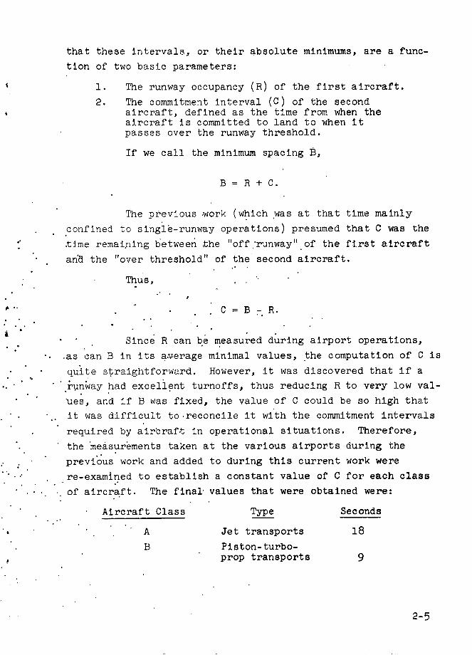
that these intervals, or their absolute minimums, are a func-

tion of two basic parameters:

1. The runway occupancy (R) of the first aircraft.

2. The commitment interval (C) of the secondaircraft, defined as the time from when theaircraft is committed to land to when itpasses over the runway threshold.

If we call the minimum spacing B,

B = R + C.

The previous work (which was at that time mainly

confined to single-runway operations) presumed that C was the

.time remai~ning between the "off 'runway" of the first aircraft

an the "over threshold" of the second aircraft.

Thus,

C=B- R.

Since R can be measured during airport operations,

as can B in its aoverage minimal values, the computation of C is

quite straightforward. However, it was discovered that if a

.runway had excellent turnoffs, thus reducing R to very low val-

*ues, and if B was fixed, the value of C could be so high that

it was difficult to.reconcile it with the commitment intervals

required by airbraft in operational situations. Therefore,

the measurements taken at the various airports during the

previous work and added to during this current work were

re-examined to establish a constant value of C for each class

of aircraft. The final values that were obtained were:

Aircraft Class Type Seconds

A Jet transports 18

B Piston-turbo-prop transports 9

2-5

Aircraft Class Type Seconds

C 8000 to 636,000 pounds

D Light twin 4engine

E All single- 0engine

It was now established that at many runways the

average minimal values of the arrival/arrival spacings were

often longer than R + C and, in fact, it became apparent that

there were inter-arrival gaps even when arrivals were spaced

at their average minimal intervals.

However, as far as arrivals are concerned, these

gaps are unusable and exist for two reasons:

1. The pilots require a "buffer" or safety marginthey can use in case of any misJudgments, espe-cially where a fast aircraft is following aslow aircraft,

2. Where a slow aircraft is following a fastaircraft, the closest the two aircraft canbe is on the downwind or base leg. Fromthis point they will become further apartso that at the runway threshold the "unusablegap" will be at the maximum.

Therefore, in our original equation,

B = R + C.

If this is maintained, by stating that although B

is the absolute minimum inter-arrival spacing, there may be a

gap (G) in the average minimum spacing (A), the following

equation applies:

A =B + G.

2-6

Since A is measurable and B is found from R and C,

both of which are known or measurable, the equation can be

solved.

If arrivals alone are examined, it is found that

FIM with the inputs of al (average value of A), a2 (second

moment of A,), and arrival rate (%,.) describes the arrival

situation and appears to give delays that correlate with real

life.

It is interesting to note the effect of runway occu-

pancy on the arrival situation. At many airports the runways

are of such a design that normally,

A >B

or

A> R+ C

However, in calculating arrival delays and/or capac-

ity on a universal basis, as was required for the Airport

Capacity Handbook, it had to be assumed that runways would

exist where their design (with respect to turnoff locations)

would be such that large average values of R could be expected.

This would be expected to affect the inter-arrival spacing so

that in these cases the following notation must be used. Where

R + C > A,

A-R+C,or

A-B.

C. RELATIONSHIP OF ARRIVAL SPACING TO DEPARTURES

The conclusions reached concerning the arrival proc-

ess have their effect on the departure process, and the effect

2-7

varies according to the design or configuration of the runways

used for arrivals and departures.

1. SINGLE RUNWAY

The task of the local controller in the tower in

handling departures on a single runway where arrivals are pres-

cnt 'i -aial a prcs 01'm-t1ating time gaps al~e

landings, and then estimating if the gaps are large enough to

clear departures for takeoff. This is basically the SAM prin-

ciple.

The interesting feature of the controller's task is

that, provided that the pilots of the arriving aircraft are

content with the spacing they have set up, the controller is

not concerned with whether each arrival spacing is a minimum

(R + C), an average minimum (A), or larger, where a natural

gap exists. As explained previously, there are unusable gaps

(that is unusable for arrivals only) and natural gaps. The

controller is interested in all gaps regardless of how they

occur. On a single runway, even with good turnoff.s, the

unusable gaps will be quite small and very few departures can

be permitted to use them--but there may be a few. Since the

controller does not differentiate between the two types of

gaps when controlling departures, it can be assumed that theJ

same rules will apply to SAM.

If there are 30 arrivals per hour at an airport and

R + C is 60 seconds average for each arrival, runway utili-

zation is 30 x 60 = 1800 seconds. -Therefore, in 1 hour there

is a further 1800 seconds total gap time, having an exponential

distribution, in which departures can be released. Naturally

departures will not be able to use the entire 1800 seconds

since there will be a probability (depending on the arrival

rate) that some of the individual gaps will not be long.enough

to release departures.

2-8

When this new concept of the input data was applied

to the original SAM, the departure delays that resulted bore

a very close relationship to actual observed delays. This was

true of the original SAM testing during the previous work and

was to be expected; the significant difference now is that

1. Average service times were used throughout,thus simplifying the generation of inputs.

2. The arrival process was more clearly under-stood and defined.

3. The model now became more adaptable for casesother than "normal" single runways.

2. INTERSECTING RUNWAYS

It should be emphasized at this point that the devel-

opment.of SAM anid its inputs, the model testing, and additional

airport surveys were all taking place concurrently. Thus,

there was continual feedback in both directions between the

model work and the surveys. The surveys, together with the

results of the model testing, are reported in greater detail

in Section TV.

At the same time that refinements of SAM for single-

runway.operations were being carried out, a start was made on

a separate but related mathematical model for intersecting

runways.. This proved to be a very complicated and difficult

task because there could be up to'three runways for such run-

way configurations, each having its own individual departure

and arrival'service times, and many additional service times

for departures and arrivals relevant to each mixture of run-

ways...

The simplification and re-definition of the inputs

to the original SAM made it appear as though the same model

could be used for intersecting runways, provided that the

inputs were correctly defined, measured, and applied.

2-9

In the previous work, a survey was made at Atlanta

airport; during this new work, Washington National airport was

surveyed. In addition, the use of intersecting runways was

studied at Chicago O'Hare and Idlewild airports. Some initial

study of these airports indicated that SAM would apply and

therefore the work on a new model was stopped.

To explain the effect of intersecting runways as

applied to SAM, it is important to establish the inputs required

and to define them. This has been partly accomplished so far,

but should now be consolidated. To ease the transition from

the previous report, the old designations are given in paren-

thesis.

T Average minimum interval between successivedepartures ($2)

F Average minimum time required to release adeparture for takeoff in front of an incomingarrival (Sll)

R Average runway occupancy for arrivals from"ov-r threshold" to "off runway" (R1 )

C Average landing commitment interval (C1)

XL Arrival rate in landings per hour ()l)

XT Departure rate in takeoffs per hour (X2 )

Figure 2-1 shows these inputs as applied to a single runway.

Using the same basic inputs, modified for intersec-

ting runways, two factors are involved:

1. Alteration of the average service times because

of runway design,

2. Alteration of the average service times becauseof individual runway use by arrivals, departures,or both (mixed operations).

In Figure 2-1, T is obtained by measuring the inter-

val from "clear to takeoff" (or "start roll") of the first

departure of a pair to the "clear to takeoff" (or "start roll")

of the second departure, where the second departure was "ready

2-10

to takeoff" before the first departure started rolling. Also,

since there is only one runway, the probability of a takeoff

on this runway being followed by another takeoff on the same

runway is obviously 1.0.

Figure 2-2 shows an intersecting runway configuration

(departures only) using both runways with an equal number of

departures on each. Also, for simplification, it is assumed

that all departures are the same type of aircraft.

In the ideal and theoretical case, a departure on

runway 1 would always be followed by a departure on runway 2,

which in turn would be followed by another on runway 1.

The value of T for 1 followed by 2 is the time

required for the departure on 1 from "clear to takeoff" to

pass through the intersection of runway 1 with 2. This is

assumed to be 30 seconds.

T for a departure on runway 2 followed by a depar-

ture on 1 would be from "clear to takeoff" to passing through

the intersection of 2 and 1. This is assumed to be 20 seconds

since the distance is shorter.

Theoretically, the final T for input to SAM is the

weighted mean of T. Since the number of departures on each

runway is equal, the probability of 1 followed by 2 is 0.5,

and 2 followed by 1 is 0.5. Thus, t1 = (30 x 0.5) +

(20 x 0.5) = 25 seconds.

However, from observations taken during the airport

surveys, it became apparent that, because of the random nature

of the departure demand (see also reference 1) there is an

equal probability of a departure on one runway being followed

by a departure on either the other runway or the same runway.

Since the interval for successive departures on the same run-

2-11

way is identical to T for a single runway (50 seconds), the

actual t1 input for this runway configuration is now:

(30 X 0.25) + (50 X 0.25) + (20 X0.25) + (50 X 0.25) w 37.5 seconds.

This very clearly shows the effect of runway design

and departure probability on the SAM inputs.

This type of approach to the formation of the inputs

was also applied to F and R and checked against actual field

data. For example, in Figure 2-2, if runway 2 was also used

by arrivals, F would be a combination of single-runway F

(takeoff on 2 followed by arrival on the same runway) and

takeoff time on 1 from "clear to takeoff" to the intersection

of 1 and 2.

Calculation of R would involve a combination of com-

plete R for arrivals on runway 2 where they would be followed

by takeoffs on 2, and a fraction of R being the time from

overthreshold on 2 to the intersection of 2 and 1 where arriv-

als would be followed by takeoffs on runway 1.

This briefly outlines the modifications made to the

SAM inputs to solve the intersecting-runway problem. The same

technique was applied to solving the Open V configurations

where operations are made toward the apex of the V. More

detailed explanations of the inputs will follow in Sections

IV, V, VI, and VII.

D. DUAL ARRIVAL FEED

At the beginning of this new work it appeared as

though it might be necessary to develop a new mathematical

model to cope with this type of operation. However, the work

which led to a redefinition of the arrival process, plus the

intersecting runway problem, led directly to the solution of

the dual arrival feed process with no extra model required.

2-12

The conclusions reached were also backed up by observations

made in the field.

Figure 2-3 A-D shows four basic types of arrival

feeds to dual runways which are, respectively:

1. A straightforward situation where there aretwo completely independent traffic patterns.

2. One basic traffic pattern but some diversionto the second runway occurring at the begin-ning of the base leg turn before turning onfinal approach.

3. One basic traffic pattern with some diversionsto the second runway but, taking place at ashort distance from the runway threshold.

4. Two basic traffic patterns but with runwaydiversion from each final approach to eachrunway.

These four patterns are based on observations made

at various airports during the field surveys. For the pur-

poses of illustration, parallel runways are shown. Except

f5or Figure 2-3D, the same procedures have also been observed

at airports having intersecting runways.

To understand the effects of such patterns on air-

port capacity one must ask the question--"Why do these differ-

ent types of patterns exist?"

From the observations taken in the field there are

three answers to this question. Diversions from one runway

to another are made by the local air-traffic controller:

1. To avoid waveoffs because the first arrival ofa pair is taking too long to exit the runway.If the controller suspects that a waveoff maybe imminent for this reason, and a seconddiversionary runway exists, he will ask thepilot of the second aircraft to break off anduse the other runway. Such procedures giverise to patterns such as those shown in Fig-ures 2-3C and 2-3D, and occasionally 2-3B.

2. To relieve the work load on himself, duringhigh arrival rates. The controller will

2-13

divert aircraft between runways to avoidthe tricky estimations of arrival spacingclose to the runway threshold. This givesrise to patterns such as those shown in Fig-ure 2-3B.

3. To promote extra gaps between successivearrivals on one runway so that departuresmay be released on that same runway. Figures2-3C and 2-3D are good examples of this, andFigure 2-3B may occur occasionally.

Having stated the reasons for these procedures, the

question can be asked--What is their effect on airport capac-

ity?

The basic operating rule observed in airport oper-

ations (and preserved in the application of the mathematical

models) is that arrivals have priority over departures. This

results in the rule that arrivals delay each other (FIM) and

arrivals delay departures (SAM), but departures do not delay

arrivals.

Examine the effect on departures first. Since SAM

evidently follows the correct rules of operation, the SAM

inputs are of interest. These inputs are:

XL Landing rate

XT Departure rate

T Departure/departure service time

F Departure/arrival service time

R Runway occupancy for arrivals

C Commitment interval for arrivals

Assume an arrival stream on a runway (1) where some

departures are waiting to take off. If some of the arrivals are

diverted to another, parallel runway (2) during their approach

to runway 1, the effect on departure delay is quite obvious.

The primary effect on the departures will be that

the landing rate (XL) on that runway (i) will be reduced.

2-14

Therefore, more gaps will be available for departures and

departure delays will be reduced. There may also be some

side effects in that, by diverting some of the arrivals to

another runway, the arrival population (mixture of aircraft

classes) using runway 1 may be altered. In this case, the

average values of F, R, and C will change because these values

are directly related to aircraft population.

Thus, provided that the number of arrival diversions

and aircraft types involved are known, the effects on depar-

tures can be computed quite simply.

Next we must examine the arrival problem. In VFR

conditions, pilots space themselves in the traffic pattern.

The traffic controller generally plays a secondary role in

that he monitors the spacing and ensures that pilots are

aware of each other and their respective intentions. The

pilots, in settling into a traffic pattern, use their judg-

ment and experience and space themselves according to air-

craft speeds and their own personal preferences. The most

critical part of the whole arrival process begins as the run-

way threshold is approached. Therefore, the whole circuit

pattern tends to hinge upon this.point.

To examine a specific case, Figure 2-3C shows one

basic circuit pattern. Assume that the primary landing run-

way (lower runway) has poor turnoffs and that runway occu-

pancy tends to be high for arrivals. If this were the only

runway available for landing it might be necessary for pilots

to allow greater spacing between aircraft. Referring to the

previous discussion of the arrival process, R + C would now

be greater than A, where A is the normal average minimal

spacing between successive pairs of aircraft. In this case,

the delay to arrivals would be higher or, for the same delay,

the number of arrivals would be lower. Thus, arrival capac-

ity would be reduced.

2-15

However, the pilots and controllers know that there

is a second runway so that, in instances where R is very large

(for the first aircraft of a pair), the second aircraft can be

diverted to the other runway. Obviously, the average minimal

value of A is still the limit because, regardless of runway

and commitment interval times, the interval A is as close as

the aircraft can comfortably get at the threshold despite the

values of R or C.

Assume an arrival population of 100 percent Class B

aircraft (piston/turboprop transports over 36,000 pounds gross

weight) on a single runway. The average interval A at thresh-

old for this class of aircraft in VFR is 64 seconds at a move-

ment rate of 30 arrivals per hour. However, if runway occu-

pancy is 60 seconds average and the commitment interval for

Class B is 9 seconds, R + C = 69 seconds. Since this exceeds

64 seconds, then either a large number of waveoffs would

have to be accepted or pilots would have to adjust their

spacings to allow for longer time intervals. Since the latter

is the more practical and safer course, these increased spac-

ings would limit the capacity of the runway.

If a second parallel or intersecting runway is

available for diversions, the average interval between suc-

cessive arrivals can be again reduced to the average value

of 64 seconds. Those combinations of aircraft pairs that

result in large values of R aftd/or C can be broken up by the

controller by diverting the second aircraft to the other run-

way.

Thus, the arrival capacity of any single runway

handling this type of traffic is 49 movements per hour pro-

vided that the average runway occupancy is 45 seconds or less.

(Section VI gives a more complete definition of arrival capac-

ity.) An average occupancy of 60 seconds would decrease capac-

ity to 36 movements per hour; However, if a second runway is

2-16

available for diversions, the arrival capacity can be expected

to increase up to 49 movements per hour--while remaining bas-

ically a single arrival circuit pattern.

Figure 2-3B shows a traffic pattern somewhere between

the extremes of Figures 2-3A and 2-3C. In Figure 2-3A, the two

circuit patterns are completely independent and can be treated

separately. Thus, long runway occupancy could affect either or

both runways. In Figure 2-3B, some of the arrivals are diverted

at a more extreme range than in Figure 2-3C and the secondary

arrival feed constitutes an almost independent operation from

the basic arrival pattern. For practical purposes in comput-

ing capacity, the independent assumption may be taken.

The only time in VFR that arrival capacity can limit

airport capacity is

1. A single runway with poor turnoffs isavailable only,

2. The arrival population includes a high per-centage of Classes A and B aircraft,

3. The number of arrivals is considerably inexcess of the number of departures.

Even under these circumstances the arrival capacity

is usually not a severe problem and any small increases in

capacity can be gained by occasional use of another runway.

For this reason, it was considered unnecessary to explore

situations such as those in Figure 2-3B in greater detail.

Finally, the question arises as to how much a sec-

ondary arrival runway will be used for arrivals when it is

available. Some study of the field data indicates that it

is very difficult to predict how much of the arrival traffic

will be diverted. This is not really surprising since the

reasons for diversion will vary from one hour to the next.

For example, in heavy arrival peak hours, diversions may be

made to ease arrival capacity and controller work load. This

2-17

may be followed by a period of lower traffic where few diver-

sions may be necessary. Again, departure peaks may give rise

to some arrival diversions to allow departures to take off.

Crosswinds, runway lengths, and the angle between intersecting

runways will all have their effects.

SubJect to these conditions, the airport observations

have shown that two basic rules apply:

1. Where one basic arrival traffic pattern is usedwith occasional diversions to a second runway,the percentage of traffic diverted to the secondrunway is not normally greater than 30 percentof the total, and values between 10 and 20 per-cent are normal.

2. If the angle between the primary and secondaryrunways is 50 degrees or less, diversions maybe expected. Angles greater than this involveconsiderable path stretching and diversionsfrom much greater ranges, which would probablyprohibit diversions on any general basis. Thereare some other considerations not mentioned hereand these are outlined in Chapter 3 of theAirport Capacity Handbook.

The effects of arrival diversion on departure delays

or capacity also should be mentioned in connection with inter-

secting runways. This, again, is impossible to state in gen-

eral terms since it depends upon where the runways intersect

with each other and the basic use of runways by arrivals and

departures. However, if the runway use is known, SAM (modi-

fied for intersecting runways as previously described) does

allow solutions.

2-18

C = COMMITMENT INTERVALR : RUNWAY OCCUPANCY

AIRCRAFT "OFF RUNWAY", AIRCRAFT READY TO TAKE O'F,

AIRCRAFT COMMITTED TO LAND NOTE THAT NO GAP IS SHOWN

F - DEPARTURE/ARRIVAL SERVICE- TIME

F

@ r -1r07-1AIRCRAFT ( TAKING OFF AND AIRBORNE, AIRCRAFT 0 AT OR

APPROACHING LANDING COMMITMENT POINT

T - DEPARTURE/DEPARTURE SERVICE TIME

T

AIRCRAFT TAKING OFF AND AIRBORNE, AIRCRAFT CLEARED TO TAKE OFF

FIGURE 2-1. SPACING FACTORS (INPUTS) FOR PRE-EMPTIVE SPACEDARRIVALS MODEL (SAM) FOR SINGLE RUNWAY

T DEPARTURE/DEPARTURE SERVICE TIME

- A

AIRCRAFT (D TAKING OFF ON RUNWAY I AND PASSING THROUGH INTERSECTION

OF RUNWAY I AND 2 AIRCRAFT Q READY AND CLEARED TO TAKE OFF

FIGURE 2-2 SPACING BETWEEN SUCCESSIVE DEPARTURES ON TWOINTERSECTING RUNWAYS

(A)

p -

(U)

(C)

(0)

FIGURE 2-3. BASIC ARRIVAL FEEDS TO DUAL RUNWAYS

III. REFINEMENTS OF STEADY-STATE MATHEMATICAL

MODELS FOR IFR OPERATIONS

IFR operations were not analyzed in any great

detail in the previous work, whereas this new study required

a solution of such operations on single, intersecting, and

close parallel runways where operations on the two runways

are not independent in IFR.

Airport surveys to gather field data required for

this new IFR analysis were made at Washington National,

Idlewild, Chicago O'Hare, and Los Angeles International air-

ports. These were carried out fairly early in the program

together with some additional VFR surveys.

The analysis of the data and adaptation of the

mathematical techniques to handle IFR operations was delayed

in order to complete the VFR modifications already described.

Since these modifications led to a simplification of the model

techniques and a greater understanding of the arrival and

departure processes, the IFR analysis was greatly eased. This

applied both to the single runway and to the intersecting run-

ways. Since the intersecting runway problem had been solved

for VFR by modifying the SAM inputs according to runway use,

it seemed logical that the close parallel combination could

be solved the same way.

However, continuous comparison was made with field

data to assure that the field data was correctly interpreted

and that assumptions were correct. This also applied to the

arrival process since it is more clearly defined in IFR than

in VFR, and delays can be measured when aircraft are being

stacked.

3-1

A large portion of the analysis of the field data

was centered on that taken at Washington National and Idle-

wild airports.

Since the inputs to the models are basically the

same in VFR or IFR, the only difference being in absolute

values and in some of the processes of formation, the inputs

will be listed again and detailed separately..

XL Landing rate per hour

XT Takeoff rate per hour

T Departure/departure service time

F Departure/arrival service time

R Runway occupancy for arrivals

C Commitment interval for arrivals

A. SINGLE RUNWAY

Since XL and kT are the demand rates, they arel not

changed by definition in IFR.

Because R and C are fairly straightforward in com-

position, they will be dealt with first.

For a given runway design (length, turnoff loca-

tions, and turnoff design), the only variations in runway

occupancy that can occur for a given type of aircraft will

be caused by: (1) variations in final touchdown speed and

(2) variations in braking action.

Since wet or slush-covered runways require pilots

to use less braking action and because such conditions often

occur during IFR--that is, cloud base 1000 feet or less and/or

3 miles or less visibility--occupancy can be expected to change

accordingly. Reference 3 indicates that, in IFR conditions,aircraft speeds at or close to touchdown are higher, so that

runway occupancy will change.

3-2

Both these factors tend to increase runway

occupancy times but the increases cannot be graded in a

simple fashion. For example, a runway may have turnoffs

located so that for VFR conditions they necessitate pilots

using limited braking to exit from the runway efficiently.

In IFR, the same turnoffs may be perfectly positioned and

no increase In runway occupancy will occur. It is possible

of course that decreases in occupancy might occur in IFR for

some runway/turnoff designs.

The commitment interval (C) can also be expected

to change in IFR conditions. The reason for this is that

since the point at which this interval starts is where the

aircraft is committed to land, low clouds or poor visibility

will require that the pilot be assured of a landing somewhat

earlier in his final approach than in VFR conditions. Also,

the pilot in VFR is usually in a position to decide for him-

self whether or not he should continue or go around, and

since he plays a large part in spacing himself from other

arrivals ahead,his Judgment can usually be expected to be

quite good.

However, in IFR the pilot can be hampered by bad

weather and increased workload in flying instruments. There-

fore, the burden of determining the "commitment to land"

point (CL) falls heavily on the local air traffic controller.

Since the controller's experience, reaction time, and radio

transmission time (to the pil.) are now involved, an increase

in C is inevitable.

During the IFR analysis, various trial computer

runs were made using fixed parameters for all the SAM inputs

except C, this input being increased by small increments for

each successive run. Since T and F are increased substantially

in IFR, the value of C can be almost doubled and still remain

a small percentage of T and F. For this reason, it was dis-

3-3

covered that SAM was not very sensitive to increases in C

over that used in VFR. This conclusion was somewhat helpful

in the analysis since C is very difficult to measure in IFR

conditions so that any estimates made in lieu of actual data

would not cause serious errors. Finally, a constant of

10 seconds was added to the VFR values of C for each class

of aircraft. Thus,

Aircraft CClass Seconds

A 28

B 19

C 16

D 14

E 10

Changes in T can also be expected in IFR because,

once aircraft are airborne, spacing must be maintained--

sometimes over quite long distances from the runway. Anal-

ysis of the field data showed that T was dependent upon the

population (similar to VFR) and upon the initial departure

routes. If only one initial route was available, large

values of T could be expected, especially where slow air-

craft are followed by fast aircraft. Where a number of

departure routes are available, separation is not so critical

since aircraft going on different routes are automatically

guaranteed separation once the airport boundary is passed.

However, there is still the probability that two departures

will follow each other on the same route, and this must

therefore be included in the formation of T.

The formation of F proved to be relatively simple

in IFR. During the airport observations it was apparent

that, when an arrival got to 2 miles from touchdown, the

controller would not release any departures for takeoff.

3-4

However, it was observed that, at any time up to this point,

a departure could be released. In fact, it was possible for

a departure to receive "clear to takeoff" up to a few sec-

onds before the arrival reached 2 miles inbound. Therefore,

the departure could still be on the runway and rolling when

the arrival was inside the 2-mile point.

However, both in the model and in real life, the

arrival is protected by the commitment interval C so that,

at the point where the arrival is committed to land, any

previous departures must be well clear of the runway. There-

fore, F in IFR for any given pair of aircraft (departure fol-

lowed by arrival) will be the time from 2 miles to "over-

threshold" for the arrival minus its commitment interval.

Interestingly enough, most of the intervals derived

in this manner seem to correlate very closely to minimums

observed during the IFR surveys, but discrepancies were found

where the intervals were between jets, or jets and piston air-

craft. In these cases, the times were even less than the VFR

minimums for F. However, a 3-mile time computation appeared

to give reasonable correlation by increasing the interval,

and this was used for the following F service times:

Class A followed by Class A

A B

A C

B A

C A

D A

E A

B. INTERSECTING RUNWAYS

As in VFR (Section II), many of the same consider-

ations will apply here with regard to the SAM inputs. The

3-5

primary considerations again are population, runway use,

and probability.

The formation of R when modified by intersecting

runways is exactly the same as for VFR. Also, C is exactly

the same as that used for single-runway operation in IFR.

The primary effects of IFR with intersecting run-

ways are in the formation of F and T.

Figure 3-1A shows a two intersecting runway con-

figuration, where the intersection is close to the runway

thresholds. From the field data, it became apparent that

the "2-mile rule" of the single runway F still holds for

this type of intersecting runway configuration. On a VFR

basis, F for the Class B aircraft departing would be the

time from "clear to takeoff" to when the aircraft passed

through the intersection (typically, 25 seconds). For the

same runway configuration and aircraft types, the "2-mile

rule" would result in an F of 43 seconds in IFR.

Now consider a runway configuration as in Fig-

ure 3-lB. Here the intersection of the two runways is at

the far end of the departure runway. The VFR F, using the

same definition of F as was used in example A is now 50 sec-

onds. The IFR F, by definition, is still 43 seconds. Thus,

a departure would still be at a point 7 seconds before the

intersection when an arrival was committed to land. Clearly,

this would violate the interval C, so in example B, the IFR F

must be the same as the VFR F.

The formation of T in IFR for intersecting runways

depends on the use of departure routings. This was very

clearly established from the field data.

Figure 3-2A shows two departures using an inter-

secting runway configuration where two fixes define two

initial departure routes.

3-6

Where the two aircraft are on different runways

and are using different departure fixes, the service time

is similar in definition to VFR T--that is, the time for the

first departure from "clear to takeoff" through the inter-

section of the two runways.

If tie two depatuoes ar using the samc departure

fix, there can be quite a significant difference in T, since

the service time no longer depends upon the runway configura-

tion but on the departure routing. Analysis of the field data

indicated that, under these circumstances, T was equivalent to

the service time for a single runway in IFR where aircraft are

using the same initial departure routing.

C. CLOSE PARALLEL RUNWAYS

To determine the effect of this configuration on

SAM inputs, it is again much easier if the actual inputs are

examined in detail.

. L and XT do not change by definition and, since

the two runways are close together, the interval C for the

arrivals does not change--in other words, this interval must

remain protected for all arrivals, whether they are preceded

by other arrivals (on the same runway).or by departures on

either runway.

The departure/departure service time (T) does not

change. Therefore, two close parallel runways are no dif-

ferent than a single runway and the same considerations of

.departure routings still hold.

Also, since the runways closely approximate the

single runway, there is normally no alteration in F. Since

the runways are closei the same considerations of waveoff

protection to the arrival apply as on a single runway.

3-7

There could be an effect on F if the landings

are confined to one runway and the takeoffs are confined

to the other runway where the two runway thresholds are not

coincident. Coincident in this case meaning longitudinally,

since there is already some lateral separation. If the

takeoff runway in such a case is "ahead" of the landing run-

way, this would relax the waveoff separation to the extent

that the 2 (or 3) mile separation would now be measured from

the takeoff runway. If the latter was 1/2-mile ahead of the

landing runway, then F would be on the basis of the arrivals

being at 1-1/2 (or 2-1/2) miles inbound. This would reduce F

in time and increase airport capacity somewhat.

Conversely, if the landing runway were ahead of the

takeoff runway, departures would require some increase in F

to ensure adequate separation. Again, this extra time is a

direct function of the longitudinal separation between the

two runway thresholds converted to time for arrivals to cover

that distance.

This effect is an assumption since no airports have

been surveyed where such a situation exists. However, the

modification was required for the analyses leading to the

handbook curves, and in the light of our general experience

in airport analyses, it is considered that the modifications

to F are realistic.

For close parallel runways in IFR, the major dif-

ference from a single runway is that the proportion of runway

occupancy (R) for arrivals, which causes delay to departures,

is quite small.

From observations taken at Los Angeles and Idlewild

(runways 4R and 7, open-V configuration where R is equivalent

to that of a close parallel configuration), it was apparent

that departures were delayed only until the arrival had touched

down on the other runway. At this point, the landing is assured

3-8

and departures need not be delayed any further. The average

time to touchdown from "over-threshold" was calculated for

the five classes of aircraft from observed data.

If all the arrivals are on one of the two runways,

and departures are confined to the other, maximum benefit

accrues from the 9hov'er effcctve runway time. If sbome

departures also use the arrival runway, then R must be

weighted by the probability of an arrival followed by a

departure on the same runway. In such a case, R will be

lengthened because the R for arrivals delaying departures on

the same runway is from "over-threshold" to "off runway."

D. ARRIVAL PROCESS

The priority rule for arrivals in VFR also applies

to IFR--that is, in the arrival/departure process, the arrivals

have priority over departures, and departures must be released

between inter-arrival gaps (SAM). In the arrival process,

arrivals may delay other arrivals (FIM).

As described in Section II, the inputs for FIM con-

sist of XL , a1 , and a2 . a1 is the average over-threshold to

over-threshold interval, and is measured when the spacing

between successive pairs of arrivals is at a minimum.

The essential difference between VFR and IFR is

that the intervals between aircraft are governed by the min-

imum 3-mile spacing required by present regulations. This

results in average spacings of greater than 3 miles in terms

of time.

As in VFR, there are combinations of average spacings

between the various classes of aircraft and the final a1 is a

weighted mean of all the intervals multiplied by their respec-

tive probabilities.

3-9

As before, the computed delays from FIM were

checked against actual delays and very good correlation

was found. A great advantage in IFR is that arrival delays

are relatively easy to measure if radar photography is

available--as it was on this project.

Delays occur mainly in the holding patterns and

delay for each aircraft is measured from the time in the

stack to the time out of the stack.

A further advantage--from the mathematical aspect--is that arrivals in IFR are confined to the ILS approach and

there are very few occasions where aircraft are broken off

and diverted to other runways, as happens in VFR.

Further aspects of the arrival process in IFR will

be dealt with in Section IV.

3-10

C - COMMITMENT INTERVALF'a DEPARTUK~ARRIVAL SER VICE TIME

2NM

C F(IFR)

"\COMMITTED TO LAND"

BOTH AIRCRAFT CLASS B

VFR F :25 SECONDSIFR F :43 SECONDS; TIME TO COVER 2 N M (62 SECONDS) MINUS C (I9 SECONDS)

(A)

~\COMMITTED TO LAND"

BOTH AIRCRAFT CLASS 9

VFR F -50 SECONDSI FR F s 50 SECONDS (SINCE TIME FOR DEPARTURE TO CLEAR INTERSECTION IS GREATER

THAN 43 SECONDS)

(s)

* FIGURE 3-1. DEPARTURE/ARRIVAL SERVICE TIME IN IFR (EFFECTOF INTERSECTING RUNWAYS)

T TIME TO RUNWAY INTERSECTION FOR DEPARTUREON RUNWAY I

0 X

0 Y 4 RUNWAY I

CLASS 1 DEPARTURE ON RUNWAY I(THROUGH FIX Y) FOLLOWED BY CLASS BDEPARTURE ON RUNWAY 2 (THROUGH FIX X)

(A)

T- IFR CLASS B DEPARTURE/DEPARTURE INTERVAL FOR

SINGLE RUNWAY VIA SAME DEPARTURE ROUTEOX

• Y I RUNWAY, I - -

CLASS 8 DEPARTURE ON RUNWAY I (THROUGH FIX X) FOLLOWED BY CLASS BDEPARTURE ON RUNWAY 2 (THROUGH FIX X)

(U)

FIGURE 3-2. DEPARTURE/DEPARTURE SERVICE TIME IN IFR (EFFECTOF INTERSECTING RUNWAYS AND INITIAL DEPARTUREROUTE)

IV. AIRPORT SURVEYS AND PERFORMANCE DATA

Sections II and III of this report have given the

ma-hemntical b ri , d an testing in very general tes.As explained, there was a continual feedback betwee, the

mathematical analysis and the field surveys.

This section will cover the field surveys in some

detail, give the actual results of the model testing, and

list the actual values of the SAM and FIM inputs as measured

during the surveys. Some of the tables of values are revi-

sions of those given in the first report, and some are com-

pletely new--particularly those applying to IFR operations.

A. METHOD OF DATA TAKING

The actual method of data taking did not materially

change from that described in the first report. The follow-

ing data was taken:

Arrivals

Aircraft type

Call sign

Runway used

Time "over threshold"

Time "off runway"

Runway exit used.

Radar Photography

Time at outer marker

Inbound route

Time in stack JTime out of stack. arrival delay

4-1

Departures

Aircraft type

Call sign

Time enter queue

Time "ready to go"

Time move out of queue toward active runway

Runway used

Time enter active runway

Time "clear to takeoff"

Time start roll

Departure route

Using two dual-track (stereo) tape recorders, it

was possible to carry out these measurements with three

observers. This is quite an advance on previous methods of

data collection. The setup used is shown at Figure 4-1. At

an airport having intersecting runways, a single runway, or

close parallel runways, observer 1 handles departures only,

while observer 2 concentrates on arrivals only. At airports

where there are wide parallel runways, each observer nor-

mally handles arrivals and departures on each runway.

Observer 3 is available as a standby--an extra pair of eyes

during peak traffic periods--and for changing the radar film

and keeping clock synchronization between the cab and the

radar camera.

It was found advisable to use our own VHF receivers

to remain independent of the tower control personnel by avoid-

ing extra cabling around the cab.

At most airports observer 1 gives departure identi-

fication and the following times: enter queue, move, enteractive, and start roll. To ease the subsequent task of data

analysis, he also logs departure identification and start roll.

4-2

This is also useful for check purposes. He also monitors his

own transmissions and the local control frequency.

Observer 2 gives arrival identification and the

following times: over threshold and off runway. He also iden-

tifies the exit used. He maintains an arrival log of identi-

fication and over threshold time, and monitors his own trans-

missions together with the departure clearance delivery fre-.

quency.

It was found that, when giving many clock times in

quick succession, errors of 5 or 1 minute were quite common

and although these were discovered during data analysis and

corrected, it was rather time-consuming. Therefore, the

latest clock used is a digital hour and minute indicator with

a large separate sweep second hand. This clock reduces errors

to a minimum.

B. DATA REDUCTION

The graphical technique used for plotting datareported on previously is still being used since it has

proved the best method. However, it has been expanded for

the IFR analysis. Figure 4-2 shows a sample of a portion of

the data taken at Washington National airport in IFR con-

ditions. On the original plot, the departure routes were

marked for the takeoffs and different colors were used for

each runway. This has been omitted here. Similar plots were

made for Atlanta, Idlewild, Chicago O'Hare, and Los Angeles

International airports.

The technique for plotting is as follows:

1. Plot time scale and set up queue areas, outermarker points, etc.

2. Plot "over-threshold" and "start roll" timesfor respective arrivals and departures usingthe hand-written runway logs.

4-3

3. Run through the arrival tape recording andcomplete arrival runway data--off runwaytime, exit used, etc.

4. Run through the departure tape recording andplot enter queue, move, enter active, andstart roll. Boundary time is an estimate tocomplete the plot, otherwise it has no sig-nificance.

5. Analyze film data and determine stack timesand outer marker times. Plot as required.

6. Using time correlation from departure track,determine the following times from the localcontrol frequency recording: ready to go calls(by pilots), and clear to takeoff. Also obtainaircraft call signs and plot as required.

7. Using time correlation from arrival track,determine clearance correct time for alldepartures from that frequency recording andplot as required.

Any weather information (visibility, wind, etc.)

and additional remarks may be added to the plot. The final

result is a very complete and easy-to-understand pictorial

display of the airport operations. From this plot, all the

required spacing intervals can be extracted with relative ease.

The reason for the "departure clearance correct" time

being taken is that, during peak traffic hours, many pilots

do not call "ready to go" until they have reached the No. 1

position for the runway. Therefore, to ensure that accurate

estimates of true ready to go times are obtained, the depar-

ture clearance time i.s required. Also, it does give a clear

indication of the delays caused by enroute congestion not

caused by the airport runways. This was not specifically

called for in this project. It was noted, for example, that

delays for departure clearance at Idlewild airport during a

survey in February 1961 were very long, while at Washington

National in March 1961 departure clearance delays were very

short, many aircraft being cleared while still taxiing out

from the terminal.

4-4

Having described the data taking and method of plot-

ting, the analysis can now be described. Each of the inputs

to the SAM and FIM models will be dealt with separately.

C. FORMATION OF INPUTS

Table 4-I gives the five classes of aircraft used

for describing aircraft types.

1. T--DEPARTURE FOLLOWED BY DEPARTURE

Definition. The interval between start roll times

(or clear to takeoff times) of successive departures measured

at the average minimum value.

The minimum value is prescribed when the second

departure is ready to go before the first departure starts

roll.

VFR

Single runway. Measurements taken during the sur-

veys completed in the previous work were added to and updated

with data from the new surveys. Table 4-II presents the

latest results. As was described in the previous report, the

intervals are subject to the pressure factor (decrease in time

intervals caused by increase in airport movements). Therefore,

the times are related to %s--being the total arrival plus

departure hourly rate.

Since completing the surveys for this project, some

additional observations have been taken at Chicago O'Hare for

the City of Chicago. These observations tend to suggest that

the T intervals, where one of the aircraft is Class A, are

4-5

somewhat less than those measured during this project. There

are three reasons for this:

1. Chicago O'Hare is being operated at capacity atthe present time and the pressure factor is veryhigh. Most of the observations taken on thisproject, where Class A aircraft were present,were at lower movement raLes (XS maxim-um, 40)though some XS of 50 to 60 were recordedrecently at O'Hare.

2. In pairs of successive takeoffs, where the sec-ond aircraft is Class A, the reduced run-uptime of many jets observed recently may permitcloser successive takeoffs.

3. Pilots and controllers are becoming more usedto larger numbers of jet aircraft. Thus,spacings are not so restrictive as they werea year or two years ago.

It should be noted that these reductions at high

XS only apply to the following aircraft class sequences: A/A,

A/B, A/C, A/D+E, B/A, C/A, and D+E/A. The latest Chicago

data was checked against the other combinations (B/B, B/C etc.)

and no differences were detected in comparison with all pre-

vious data.

Intersecting runways, including open V (operations

toward the apex). A combination of two time intervals--"clear to takeoff" to start roll, plus "start roll" to

desired intersection. The latter is measured from the run-

way threshold. Table 4-II gives "clear to takeoff" to

"start roll" average intervals for the five aircraft classes

from the data. It was observed that the pressure factor did

have some effect on these intervals, but it was very slight

and was ignored for practical purposes.

It snould be noted that the figure of 18 seconds

for Class A is based on data accumulated up to March 1962.

Some very recent observations have indicated that this average

may have since become about 9 to 12 seconds. The reason for

4-6

this is that pilots are becoming more familiar with the jets

and rolling takeoffs are becoming common. Also, the percent-

age of jets requiring long engine run-up periods for water

injection is decreasing rapidly.

The time from "start roll" to a given intersection

distance is mainly a function of the aircraft type. Fig-

ures 4-3 through 4-7 show time versus distance for Classes A

to E.

IFR

Single runway. T is defined in the same way as VFR

except that there can be two separate values depending upon

whether each pair of departures are on the same initial depar-

ture route or proceeding on different routes.

Tables 4-IV and 4-V give the final results as deter-

mined from the field data. Table 4-IV gives the intervals

where successive aircraft are using the same initial depar-

ture route, Table 4-V for different departure routes. It

will be noticed that, for some aircraft combinations, the

departure intervals in IFR for different departure routes are

the same as the VFR intervals.

Intersecting runways. Here the use of departure

routes governs the departure spacings in IFR. If two suc-

cessive departures are using the same initial departure route

fix, the interval will be based on that fact regardless of

the runway used. This became very clear from the analysis of

the Washington data, where all takeoffs from runway 3 used

the Riverdale departure fix. Where such takeoffs were fol-

lowed by a takeoff on runway 36 going via Riverdale, the take-

off intervals were relatively long. Where the takeoffs on

runway 36 were routed through the Georgetown fix, the run-

way 3/36 intervals were the same as in VFR--that is, the

4-7

time for a takeoff on runway 3 from "clear to takeoff" to pass-

ing through the intersection of runways 3 and 36. Therefore,

Table 4-II1 and Figures 4-3 through 4-7 should be used in such

cases.

2. F--DEPARTURE FOLLOWED BY AN ARRIVAL

Definition. The average minimal time re-qared to

release and clear a departure in front of an incoming arrival.

VFR

Single runway. F for single runways in VFR is very

difficult to measure. At high movement rates, absolute mini-

mums can be observed where on occasion the controller will

release a departure very close to an incoming arrival. Since

a great deal of field data has been accumulated during this

and the previous work it was not too difficult to establish

the absolute minimums. It would, however, be desirable to

increase the data for these minimums where jet aircraft are

involved, but there is enough at the present time to establish

reasonable figures.

Measurement of the inter-arrival gaps where depar-

tures are ready to go but are not released also provides addi-

tional evidence as to minimum F. From this data it is evident

that F is subject to the pressure factor.

Measuring the inter-arrival gaps between arrivals

where a departure is released provides an indication of F

maximum.

With a knowledge of F minimum and F maximum, it was

found that the equation

F - T - 2C

4-8

gives a satisfactory solu.tion for F. Also, F is still limited

to its minimum values (already known) if the equation gives a

solution less than F minimum. Table 4-VI gives minimum values

of F for all aircraft class combinations. The equation has

been used in all the latest testing of actual versus computed

delays and appears to give a satisfactory answer.

Intersecting runways. The calculation of F is quite

straightforward here, being identical to T in VFR--that is,

the time from "clear to takeoff" to passing through the inter-

section of the takeoff and landing runway. Table 4-III and

Figures 4-3 through 4-7 can be used to calculate F as required.

IFR

Single runway. The 2-mile rule described in Sec-

tion III applies here. Table 4-VII gives the values of F for

each aircraft class combination.

Intersecting runway. Section III gives a complete

description. Table 4-II and Figures 4-3 through 4-7, or

Table 4-VII, can be used to calculate F as required.

3. R--RUNWAY OCCUPANCY FOR ARRIVALS

Definition.

1. Arrival followed by arrival on the same runway.Runway occupancy from "over threshold" to "offrunway" for the first aircraft in every pairof aircraft.

2. Arrival followed by departure on the same run-way. Runway occupancy from "over threshold"to "off runway" for the arrival.

3. Arrival followed by departure on intersectingrunways other than open V configurations.Runway occupancy from "over threshold" to theintersection of the arrival and departure run-way, except in cases where the intersection istoward the far end of the arrival runway. Insuch cases where the arrivals mostly exit

4-9

before the intersection, the field data indi-cates that the effective runway occupancyceases as the arrival begins to start to exitthe runway. This occurs about 7 to 12 sec-onds before the actual "off runway" time. Inother words, the controller can release adeparture before the "off runway" of the arrival.Figures 4-8 through 4-12 show the time fromover-threshold versus distance from runwaythreshold for the five classes of aircraft.For each class, the time also varies as afunction of runway length. Therefore, variousgroups of runway length are shown on each fig-ure. These results are also taken from ananalysis of the field data.

4. Arrival followed by departure on intersectingrunways where the intersection is beyond therunways--that is, open V configurations onoperations toward the apex. Also close par-allel runways in IFR. Here the field dataindicates that the effective runway occupancyfor the arrivals is now time from over thresh-old to touchdown.

Tables 4-VIII and 4-IX give the values for each

aircraft class in VFR and IFR.

The computation of runway time for runway config-

urations is generally quite straightforward where only a

portion of the total runway occupancy is of interest. How-

ever, since the very beginning of this airport capacity work,

the computation of total runway occupancy--that is, from"over threshold" to "off runway"--has always eluded a simple

analysis.

If a runway is in existence and being used, it is

a simple (but time-consuming) task to take a number of obser-

vations and calculate the average runway occupancy for each

aircraft class. However, this is complicated by the fact that

the field data indicates that, as the landing rate increases,

the average runway occupancy time decreases. Again, this is

the effect of the pressure factor. Thus, a simple measure-

ment of runway occupancy time at a XL of 10 landings per hour

could be expected to be less at a XL of 20.

4-lo

Therefore, it was decided quite early in the begin-

ning of this work that a definition of runway rating should

be adopted.

A detailed examination of the field observations

was first undertaken to calculate a series Of curves that

would show the effect of pressure factor. Figure 4-13 shows

the family of curves that resulted from this analysis. Use

of these curves is best illustrated by an example.

Example. Field observations at an airport show an

average runway occupancy of 47 seconds at a XL of 15 landings

per hour. What will the runway occupancy be at a XL of 30

landings per hour? Enter left-hand vertical scale of 47 sec-

onds. Intersection of XL 15 occurs on the 45 rating curve.

Follow this curve to intersection with XL of 30. Now read

off the new runway occupancy from the left-hand vertical scale

(43 seconds).

Notice that the pressure factor has a greater effect

on runways which have poor runway occupancy times than on

those with good occupancy times.

All these curves were plotted from a known equation.

Thus, if a fixed XL of 20 landings per hour is used as a ref-

erence line it is possible to specify the runway rating

at XL 20 as an input to the equation. Therefore, the complete

curve for runway occupancy versus XL is known. This technique

allows two simplifications:

1. It allows a simple definition of runway occu-pancy by giving a runway rating.

2. It is readily adaptable to a computer program.

However, this only applied to runways where it was

possible to measure occupancy by means of a survey. When

analyzing airports not yet built, and preparing the airport

capacity handbook, it was necessary to predict runway rating.

4-11

Also, because it was hop.ed.to keep the handbook presentation

as simple as possible, an uncomplicated method of prediction

was required.

Some further analysis of the field data led to a

solution. It was reasoned that, while individual pilots vary

in their landing technique and there are differences between

individual aircraft within the five class groupings, it should

be possible to determine an exit range for a given class of

aircraft. An exit range may be defined as the range of dis-

tance along the runway (measured from the threshold) within

which the aircraft are in a position, and at such a speed

that, if exits are provided within the range they can be used.

Having presumed that this is a logical assumption,

leads to the conclusion that the greater the number of exits

within the exit range, the lower the runway occupancy.

Two factors could be expected to alter these assump-

tions:

1. Effect of airport altitude would increase air-craft true airspeed at touchdown and alsolessen effects of propeller or Jet braking.

2. Runway length was already known to affectlanding performance--the greater the runwaylength, the less severe is the pilot's brak-ing action.

Because of these factors, the field data was first

grouped by runway length and only VFR data from airports whose

elevation was less than 1000 feet was considered. Also, only

runways having right-angle turns were initially considered.

From the previous work, some estimation of exit

ranges by class and runway length was possible. Using these

estimations and the actual runway occupancies from the data,

we correlated the number of exits available within each exit

range with the actual runway occupancies. After several tries,

~4-12

making small adjustments each time, it was possible to predict

runway occupancies of actual runways to within 5 seconds or

less on the average.

This left the problem of wet runways, altitude, and

high-speed turnoffs. For the latter, the basic technique is'

similar to right-angle turnoffs except that the exit range

is closer to the threshold since aircraft are in a position

to use high-speed turnoffs at a speed of 60 mph. In the pre-

vious report (reference 1), a considerable amount of work was

done on determining the range of this 60-mph point for various

classes of aircraft (based on references 3, 4, and 5). This

proved invaluable in the calculations. Again, the technique

was used to predict runway occupancies at airports where such

runway data was available on high-speed turnoffs. These were

notably Idlewild and Los Angeles International. In addition,

a further analysis was made of runways having angled turnoffs--

that is, turnoffs between the right-angled and high-speed types.

Finally there was the aspect of altitude and wet

runways (IFR). Since the main effect on the aircraft is to

increase the distance along the runway to where the exit range

is reached, which is similar to the effect of increasing run-

way length, it was felt that these parameters could be han-

dled by giving a correction factor to runway length.

For the altitude effect, a study of reference 6 and

aircraft performance data yielded the required information on

increases in runway length. This allowed a graphical solution

of runway correction factor versus airport altitude and air-

craft class that was then tested with the runway occupancy

data obtained at Denver (elevation, 5331 feet) and reasonable

predictions were obtained.

For IFR or wet runways,.a correction of 1.1 (10 per-

cent increase) was applied to runway lengths. This was deter-

4-13

mined on a trial and error basis using runway data from run-

ways 36 and 4R at Washington and Idlewild, respectively.

The final graphs, tables, and explanation of the

technique as applied to actual cases is contained in the

Airport Capacity Handbook. Therefore, these aspects will

not be covered here.

4. C--COMMITMENT INTERVAL FOR ARRIVALS

Sections II and III of this report describe the

analysis leading to the definition of C in VFR and IFR. There-

fore, no further discussion is required here.

5. A--ARRIVAL FOLLOWED BY ARRIVAL (FIM MODEL ONLY)

Definition. The interval between successive pairs

of arrivals measured at the runway threshold when the spacing

is at its average minimum value.

The average minimum value is assured in VFR when:

1. The second arrival is seen to perform any path-stretching maneuvers during downwind, base, orfinal legs.

2. Two arrivals are both on final approach togetherin a normal traffic pattern (that is, wherearrivals do not come straight in but carry outnormal downwind, base, and final legs).

3. A departure is ready to go but not releasedbetween two successive arrivals.

The average minimum value is assured in IFR when:

1. The second arrival is seen to be stacked,orbited, or path-stretched before the runwaythreshold.

2. A departure is ready to go but not releasedbetween two successive arrivals.

3. Two or more arrivals are being stacked. Anyintervals occurring during such periods oftime can be regarded as average minimums,whether or not any of the aircraft making upthe intervals have been stacked themselves.

4-14

Having specified the conditions for measurement of

A intervals, the following comments apply.

VFR

As for most of the model inputs, A is affected by

the pressure factor. Thus, there is a decrease of A with

increasing L. The previous report gave a table of values

for the various aircraft class combinations which has been

updated and revised in this report as Table 4-X.

IFR

The new data in Table 4-XI gives the results of the

measurements obtained from the IFR surveys.

Several points are of particular interest here.

Pressure factor does affect the interval A in IFR.

From the data gathered so far, the reduction in service times

parallels the VFR case. Figure 4-14 is a comp6site graph show-

ing this effect.

The graph shows A (time) versus XS (total movement

rate) for Class B followed by Class B. The horizontal hatched

lines show the values for A for 3- and 5-mile average spacings

between successive aircraft. The dots are individual spacings

taken direct from the field surveys under IFR conditions.

The lower curve shows the basic VFR A. When the

average values of each set of IFR spacings were plotted, it

was evident that a curve paralleling the VFR curve, but greater

by 61 seconds, passes through or close to the IFR averages.

The top curve is, therefore, the average interval A for Class

B followed by Class B in IFR.

4-15

. . .. . . . ... . .

Another interesting feature here is that, at the

higher movement rates, the average IFR spacing is quite close

to the specified 3-mile rule. It will be seen that some

intervals apparently fall below the 3-mile line. This should

not be construed as necessarily violating the rule in every

case, since the 3-mile line is an average based on Class B

aircraft average speeds. Some aircraft cover 3 miles some-

what faster than others and, therefore, fall below this

3-mile line.

What it does indicate is that the approach controllers

are performing very well with these types of aircraft; the aver-

age spacing at the higher movement rates being 3-1/2 miles.

Where jet aircraft (Class A) are concerned, there is

a general lack of data at the higher movement rates (above XS 25)

but the data gathered on this project indicates that average

intervals between Class A aircraft are in the order of 6 miles.

Recent surveys taken at Chicago O'Hare for the City of Chicago

tend to suggest that spacings there may be somewhat less than

this for Class A aircraft. This has not been confirmed, but

it does indicate that data collection of this sort ought be

done fairly regularly at such airports if the model inputs are

to be kept up-to-date.

Theoretical analysis. Many analyses of IFR approach

feeds and capacities done in the past have assumed that the

-length of the common path (ILS) will have an effect on capac-

ity since spacings between aircraft having dissimiliar speeds

will be necessarily increased on long common paths. This

seems to be a valid theoretical assumption.

However, an analysis of the radar photography and

time data from the surveys indicate that this apparently does

not have a major effect. For example, it would appear at

first sight that the length of common path at Los Angeles is

twice that of Washington National. At Los Angeles, the air-

4-16

space approaching the airport (runways 25L and 25R) is very

restricted because of adjacent airports and mountains, and

the majority of arriving aircraft are coming from the east.

However, by means of radar vectoring and speed control, the

approach controllers can bypass fast aircraft around the slow

ones; in many cases, the light aircraft are kept clear of the

ILS until the last possible movement consistent with safety.

Also, at Washington National, aircraft were vectored onto the

ILS in such a way that there was, in effect, no common path

beyond the outer marker in many cases. The same is true at

Idlewild.

There is not enough data yet to absolutely prove

that the length of common path does not affect capacity,

but the evidence so far suggests that controllers use tech-

niques to avoid the effect.

Another question has arisen many times during the

VFR and IFR analyses, both in this and the previous work--do

poor controllers have an adverse effect on capacity?

First, it should be stated that when performing a

capacity analysis, especially where it leads to an economic

analysis of airport design, one cannot plan on anything other

than the average controller. Obviously "good" or "bad" con-

trollers could only have short-term effects on airport capac-

ity even if this were true.

The VFR analyses so far have shown that there are

few if any such effects. This is partly because of the fact

that the pilots are also involved, and the combination of"good controllers" and "bad" piloting is just as likely as

both being "good" or vice versa.

From the data taken in IFR, it appears that the

same is true, but here the evidence is not as clear as in VFR.

There is a suggestion that, if the controllers are not

4-17

restrained by local traffic rules (imposed on top of the uni-

versal traffic procedures) or by such things as a lack of

departure routes, then there may be a learning factor as

applied to the Jet aircraft. In other words, there is some

evidence (as yet unchecked) that high movement rates at some

airports in IFR are inducing higher learning rates among those

controllers, and spacings are being reduced within the rules--

at least those involving Jet aircraft. One reason for this

is perhaps that the controllers are using speed control intel-

ligently and in fact they are being encouraged to do so.

At one airport, controllers have recently been

instructed to use 6-mile minimum spacing on arrivals on one

particular runway to alleviate the noise problem. If this

rule is followed, reduced capacity and/or increased arrival

delays are unavoidable. An added side effect is that the

controllers will not have the opportunities to get used to

high movement rates and poorer performance is inevitable.

Also, it should be repeated that, in discussing

aspects of common path lengths, there is a definite effect

on departure capacity as already observed. However, at

Idlewild on runway 31L, recent surveys (conducted under Con-

tract FAA/ARDS-605) have indicated that departure capacity

on this runway is most severely restricted because there is

but one departure route and its length is much longer than

observed at any other airport. This does seem to have a seri-

ous effect. Another aspect should be mentioned. Chicago

O'Hare is preserit.y faced with very high traffic demands

coupled with a relatively low capacity airport configuration

under certain wind conditions. When the wind is from the

west arrivals can use runway 32L (length 11,600 feet) but can-

not use 32R because this would result in excessive delays to

departures on that runway. Also, the number of arrivals on

32L has to be limited because of the departures on that runway

as well.

4-18

The ideal situation is to allow some arrivals on

32L and the remainder on runway 27, and departures on 32L

and 32R. Until recently the air traffic procedures did not

allow independent traffic patterns on 32L and 27. Therefore,

this would not have allowed maximum use of these runway for

arrivals. However, as a special case, the rules have now been

changed for O'Hare to allow this provided that weather con-

ditions are more than 2500 feet of cloud base, and more than

6 miles visibility, together with some coordination between

the two runways.

This leads on to the final point. The SAM/FIM model

combination has proved its validity in giving answers consist-

ent with airport surveys. If the air traffic control rules

change, or operational procedures or practices change, they

do not make the model unusable. Such changes only affect the

inputs to the models and, provided that the effect of such

changes is either measured (in the field) or correctly assumed,

then airport capacity and/or delay can be correctly computed.

With this in mind it has become apparent that the

technique of field surveys with proven models is a most power-

ful tool for airport design studies.

D. MODEL TESTING

Table 4-XII gives the final results of the model

testing, where the actual observed delays have been compared

with computed delays. The computed delays have been calcu-

lated using the full IBM 7090 computer program (Section VI)

and incorporating the mathematical model and input routines

described in Sections II, III, and V.

All these tests are the result of the new surveys

conducted during this recent project with the exception of

Wichita and Miami, which were completed on the previous con-

tract. For check purposes, these two cases were re-runs using

4-19

the full computer program. In the previous report, Wichita

had a computed delay of 0.6 minute. The computed delay with

the new program is 0.5 minute (actual delay, 0.2 minute).

The Miami test previously gave a computed delay of

4.6 minutes against 2.8 minutes actual delay. This was the

worst correlation of all the previous test cases and though

statistically valid (from the purely mathematical aspects),

it was not a close correlation in the practical sense.

The Miami case was of particular interest becauseduring that particular survey there was some use of inter-

secting runways though the majority of aircraft used a sin-

gle runway. During the previous testing, there was some

difficulty in running tests on intersecting runways. There-

fore, this example was run as though it was a single runway

only.

Using the full computer program, which allows auto-

matic computation of inputs for many runway configurations,

the Miami case was run as it actually existed during that

survey. Table 4-XII shows that the computed delay is now

3.1 minutes compared with 2.8 minutes actual delay.

This case is interesting in that it shows the advan-

tage of intersecting runways over single runways (provided

that the runway intersections are favorably located); the sin-

gle runway resulted in a much higher figure of delay than did

the intersecting runway.

The model testing was used to check the validity of

application of the finally accepted models, and to refine

the definition of mode] inputs through a recycling procedure.

The models were tested against actual operations. Spacing

factor inputs were then refined to improve correlation and

these refinements incorporated into the composite compila-

tion of' spacing factor inputs. The models were then retested

using the composite of spacing factors.

4-20

An example of the Washington National IFR analysis

will illustrate this. After completion of data taking and

data reduction for Washington, the initial spacing factors

were determined. These factors (from National data only)

were used for initial testing of the models. The initial

testing indicated better agreement should be obtained, so

the operation was re-analyzed to determine that some redefi-

nition of spacing factors was necessary. For example, the

effect of departure routings and how to provide for this

effect was learned through this process. When reasonable

agreement was attained for the Washington test period, IFR

operations at other airports were analyzed. Gradually the

spacing factors from those airports that were surveyed were

summed into a composite curve for each factor expressed in

time versus movement rate (to include the pressure factor).

The composite curve was programmed as part of the computer

program for generation of model inputs. Finally, the Wash-

ington National observation period was retested using the

computer program of composite spacings. The correlation

obtained between computed and actual delay is shown in

Table 4-XII. Table 4-XIII repeats the results of the

model tests included in the first phase of the contract

(reference 1). Not all of these cases were retested under

the present phase. Where retesting has been accomplished,

it has been done using the broader input data or spacing

factors now available.

The model inputs as gradually developed and

assembled have become a broad enough sampling to represent

a national standard measure of the input values. The model

tests appearing in Table 4-XII are those performed at the

end of the process of testing and sharpening input data.

They are thus indicative of the correlation to be antici-

pated if one goes to any civil U.S. airport and performs

4-21

the necessary field observations, data reduction, and model

computations. Should the correlation not be good--say the

delay observed is markedly less than the model prediction--

one can anticipate that closer study will show an unusual

performance is being accomplished which has reduced input

values for that case. The comments under previous section Cl

on O'Hare observations illustrate this point.

Since the model inputs are based on current meas-

ured data, they should be checked periodically by additional

field observations, for the spacing factors may change as

new procedures are developed and as the operation of new

aircraft becomes routine. Broadening of observed data for

IFR operations of heavy jet aircraft would be particularly

desirable as the data available during the field work of

this contract has been more limited than would be desirable.

Further, IFR procedures and performance are gradually being

improved to increase IFR capacities.

4-22

TABLE 4-I

AIRCRAFT BY TYPE AND CLASS

Class Description Type

A All Jet aircraft nor- Boeing 707 and 720 seriesmally requiring runway Douglas DC-8 series.lengths in excess of Convair 880 and 9906000 feet for takeoff Sud-Aviation Caravelleand/or landing (cor- DeHavilland Cometrected to sea level). BAC VC 10

B (1) Piston and turbo- BAC lllprop aircraft having Boeing 727a normal loaded weight Lockheed Jetstarof >36,000 pounds Lockheed Electra(2) Jet aircraft not BAC Vanguardincluded in Class A Vickers Viscountbut having a normal Douglas DC-6 andloaded weight DC-7 series>25,000 pounds. Lockheed Constellation

Bristol BrittanniaConvair 240, 340, and 440Martin 202 and 404

C (1) Piston and turbo- Fairchild F-27prop aircraft having Grumman Gulfstreama normal loaded weight Douglas B-26of >8000 pounds but Lockheed Lodestar and<36,000 pounds. Learstar series(2) Jet aircraft having Douglas DC-3a normal loaded weight Beech 18 seriesof >8000 pounds but North American T-39<25,000 pounds Potez 840

Aero Jet CommanderDeavilland 125

4-23

TABLE 4-I (cont)

Class Description Type

D All light twin-engine Beech 500 Twin Bonanzapiston/turboprop air- Aero Commandercraft with <8000 pounds Beech Queen Airnormal loaded weight Beech Travelairand some high-perform- Piper Aztecance single-engine light Piper Apacheaircraft. Cessna 310

Cessna SkyknightBeech Bonanza andDebonair

DeHavilland Dove

E All single-engine light Piper Cub, Tripacer,aircraft other than Pacer, etc.those included in Cessna 140, 150, 170,Class D 180, and 210 series

Piper CherokeePiper Comanche

Beech MusketeerDeHavilland Beaver (L-20)Mooney M20Aeronica Champion

4-24

TABLE 4-I1

T, AVERAGE MINIMUM SPACING BETWEEN SUCCESSIVEDEPARTURES ON SAME RUNWAY (VFR)

Class A f/b* Class A Class A f/b* Class BT XT

S (second) s (second)

20 72.0 20 79.030 69.8 30 76.840 68.0 40 75.050 67.0 50 73.860 65.8 60 72.870 65.0 70 72.280 64.2 80 71.290 63.5 90 70.5100 63.0 100 70.0110+ 63.0 110+ 70.0

Class A f/b* Class C Class A f/b* Class D & E

T TS (second) Xe (second)

20 83.2 20 85.530 74.8 30 78.540 69.4 40 73.550 65.5 50 70.460 62.5 60 67.570 59.8 .0

80 ~57.8 ;90 55.8 90 64.0100 55.0 100 64.o110+ 55.0 110+ 64.0

Movement rate (xs) values are given up to x = 110, but thisshould not be interpreted as being of any significance otherthan the fact that it shows the full range over the curve.For example, a runway handling all Class A aircraft wouldreach capacity well before a Xs of 110 movements per hour.However, at an airport handling only 1 percent Class A air-craft and a large population of Class D and E aircraft, thecapacity could well approach Xs - 110 movements per hour.

= movement rate.s

T = average minimum spacing between successive departures.* f/b = followed by.

4-25

TABLE 4-I (cont)

Class B f/b'Class A Class B, f/b* Class BT T8S (second) s (second)

20 8o.4 20 81.530 76.0 30 71.040 73.8 40 64.550 71.5 50 6.o60 69.8 60 56.270 68.4 70 53.580 67.2 ;o 51.090 66.o 90 49.o100 65.3 100 48.0110+ 65.0 110+ 48.o

Class B f/b* Class C Class B f'A Classes D & E

T Ts (second) Xs (second)

20 59.0 20 77.530 54.6 30 63.840 51.5 40 55.850 49.2 50 49.560 47.5 60 45.570 46.0 70 42.480 45.o 80 39.890 45.0 90 39.0100 45.0 100 39.0110+ 45.0 110+ 39.0

Class C f/b* Class A Class C f/b* Class BT TXs (second) Xs (second)

20 100.5 20 71.030 91.0 30 63.540 84.6 40 58.550 80.5 50 55.060 77.0 60 52.2o 4.4 0 50.0

077.0 ;o48.090 69.8 90 46.5100 68.0 100 45.5110+ 67.0 110+ 44.0

4-26

TABLE 4-I (cont)

ClassesClass C f/b* Class C Class C f/b* D and ET T

(second) s (second)

20 54.5 20 54.430 53.8 30 45.540 44.8 40 39.650 42.0 50 36.060 39.5 60 33.370 37.8 70 31.280 36.5 80 31.090 35.5 90 31.0100 35.0 100 31.0110+ 35.0 110+ 31.0

Classes ClassesD and E f/b* Class A D and E f/b* Class B

T T(second) s (second)

20 94.5 20 59.030 90.3 3o 55.540 87.8 0 52.550 85.5 50 50.560 83.6 60 49.070 82.2 70 48.080 81.2 0 46.690 80.o 90 46.0100 79.0 100 46,0110+ 78.3 110+ 46.0

Classes Classes ClassesD and E f/b* Class C D and E f/b* D and ET T

(second) (second)

20 68.0 20 5J.530 53.8 04o40 45.5 3.50 40.0 50 38.260 36.0 60 34.070 34.o 0 28.880 34.0 80 27.09o 34.0 90 25.4100 34.0 100 24.0110+ 34.0 110+ 23.0

4-27

TABLE 4-iII

TIME FROM "CLEAR TO TAKEOFF" TO"START ROLL" FOR DEPARTURES

TimeAircraft Class (second)

A 18

B 9

C 8D 4E 4

4-28

TABLE 4-IV

T, AVERAGE MINIMUM SPACING BETWEEN SUCCESSIVEDEPARTURES ON SAME RUNWAY AND SAME DEPARTURE ROUTE (IFR)

Class A f/b* Class A Class A f/b* Class B

T Ts (second) s (second)

10 94.2 10 85.220 90.0 20 81.230 87.5 30 79.040 86.0 40 77.050 86.0 50 77.060+ 86.0 60+ 77.0

Class A f/b* Class C Class A f/b* Classes D & E

T Txs (second) Xs (second)

10 100.8 10 96.820 83.2 2.0 85.530 74.8 30 78.540 69.4 40 73.550 67.0 50 70.460+ 67.0 60+ 67.5

Class B f/b* Class A Class B f/b* Class B

T T_S (second) s (second)

10 114.5 10 110.020 107.0 20 89.030 102.5 30 78.540 100.0 4o 72.050 100.0 50 69.060+ 100.0 60+ 69.0

T = average minimum spacing between successive departures.

k= movement rate.5* f/b = followed by.

4-29

TABLE 4-Iv (cont)

Class B f/b* Class C Class B f/b* Classes D & E

T Ts (second) Xs (second)

10 79.0 10 108.320 69.4 20 77.530 65.2 30 63.840 62.0 40 55.850 59.8 50 49.560+ 59.0 60+ 45.5

Class C f/b* Class A Class C f/b* Class B

T Ts (second) Xs (second)

10 145.5 10 129.020 126.4 20 113.630 117.3 30 lO6.o40 111.0 40 101.050 111.0 50 101.060+ 111.0 60+ 101.0

Class C f/b* Class C Class C f/b* Classes D & E

T Ts (second) Xs (second)

10 97.0 10 103.820 84.5 20 84.230 78.0 30 75.540 74.0 40 69.550 73.0 50 67.060+ 73.0 60+ 67.0

Classes ClassesD and E f/b* Class A D and E f/b* Class B

T Ts (second) s (second)

10 157.0 10 14 .020 150.2 201 136.030 146.0 30 131.540 143.0 40 129.050 143.0 50 129.060+ 143.0 60 129.0

4-30

TABLE 4-IV (cont)

Classes ClassesD and E f'/b* Class C D and E r/b* Classes D & E

T TXs (second) ~ s (second)

10 133.8 10 114.520 100.0 20 91.230 100.0 30 81.840 100.0 40 76.050 100.0 50 75.06o+ 100.0 60+ 75.0

4-31

TABLE 4-V

T, AVERAGE MINIMUM SPACING BETWEEN SUCCESSIVE DEPARTURESON SAME RUNWAY BUT ON DIFFERENT DEPARTURE ROUTES (IFR)

Class A f/b* Class A Class A f/b* Class B

T Txs (second) Xs (second)

10 76.0 10 83.220 72.0 20 79.030 69.8 30 76.840 68.0 40 75.050 67.0 50 73.860+ 65.8 60+ 72.8

Class A f/b* Class C Class A f/b* Classes D & E

T T3 (second) s (second)

10 oo.8 10 96.820 83.2 20 85.530 74.8 30 78.540 69.4 40 73.550 65.5 50 70.46o+ 62.5 60+ 67.5

Class B f/b* Class A Class B f/b* Class B

T TXs (second) s (second)

10 100.5 10 102.620 93.0 20 81.530 88.5 30 71.040 86.0 40 64.550 86.0 50 60.060+ 86.0 60+ 56.2

T = average minimum spacing between successive departures.

k= movement rate.* f/b = followed by.

4-32

TABLE 4-V (cont)

Class B f/b* Class C Class B f/b* Classes D & ET %T

S (second) 8 (second)

10 68.5 10 lO8.320 59.0 20 77.530 54.6 30 63.840 51.5 40 55.850 49.2 50 49.56o+ 47.5 6o+ 45.5

Class C f/b* Class A Class C f/b* Class B

T TS (second) s (second)

10 125.5 10 97.520 106.3 20 82.030 97.3 30 74.440 91.0 40 69.650 91.0 50 67.o60+ 91.0 60+ 67.0

Class C f/b* Class C Class C f/b* Classes D & E

T TXs (second) "s (second)

10 80.5 10 90.020 68.0 20 70.830 61.6 30 62.040 57.4 40 56.050 55.0 50 52.860+ 52.6 60+ 50.0

Classes ClassesD and E f/b* Class A D and E f/b* Class B

T Ts (second) s (second)

10 131.2 10 104.220 124.3 20 96.830 120.0 30 92.640 117.2 40 90.050 116.o 50 90.060+ 116.o 60+ 90.0

4-33

TABLE 4-~V (cont)

Classes Class DD and E f/b* Class C and E f/b* Classes D & E

xT Ts(second) Xe(second)

10 114.2 10 94.020 80.8 20 71.030 68.0 30 61.240 68.0 40 55.550 68.0 50 52.060+ 68.0 6o+ 52.0

4-34

TABLE 4-VIABSOLUTE MINIMUM VALUES OF F FOR SAME RUNWAY (VFR)

Aircraft AircraftClass Class F min

(Departure) (Arrival) (secl

A followed by A 51A B 60A C ,64A D 67A E 75B A 38B B 32B C 36B D 39B E 45C A 39C B 29C C 29.C D 32C E 40D A 38D B 30D C 24D D 20D E 22E A 38E B 30E C 24E D 20E E 21

F = departure release in front of an incoming arrival.

4-35

TABLE 4-ViIAVERAGE MINIMUM VALUES OF F FOR SAME RUNWAY (IFR)

Aircraft AircraftClass Class F

(Departure) (Arrival) (sec)

A followed by A 56A B 74A C 83A D 66A E 86B A 56B B 43B C 50B D 66B E 86C A 56c B 43C C 50C D 66C E 86D A 56D B 43D C 50D D 66D E 86E A 56E B 43E C 50E D 66E E 86

F = departure release in front of an incoming arrival.

4-36

TABLE 4-vlll

AVERAGE TIME FROM OVER-THRESHOLD TO RUNWAY TOUCHDOWNFOR ARRIVALS IN VFR (EQUALS VALUE OF R FOR OPEN-V RUNWAYS)

Runway Length (feet)

5301 6200 7001 9501Aircraft to to to to to

Class 5300 6199 7000 9500 12,999 t13,000

A 6.,0 7.0 7.0 7.5 8.0

B 5.0 6.0 7.0 8.0 8.0 8.0

C 5.0 7.0 8.5 10.5 10.5 10.5

D 5.0 7.0 8.5 10.5 10.5 10.5

E 5.0 8.0 11.o 14.0 14.0 14.0

All times in seconds.

R = runway occupancy for arrivals.

4-37

TABLE 4-ix

AVERAGE TIME FROM OVER-THRESHOLD TO RUNWAY TOUCHDOWNFOR ARRIVALS IN IFR (EQUALS VALUE OF R FOR

OPEN V AND CLOSE PARALLEL RUNWAYS)

Runway Length (feet)5301 6200 7001 9501

Aircraft to to to to toClass 5300 6199 7000 9500 12,999 13,000

A 8.0 10.0 10.0 10.0 11.0

B 10.0 12.0 14.0 17.0 17.0 17.0

C 14.o 16.0 18.0 20.0 20.0 20.0

D 15.0 16.0 18.0 20.0 20.0 2Q.O

E 21.0 24.0 26.0 29.0 29.0 29.0

All time in seconds.

R = runway occupancy for arrivals.

4-38

TABLE 4-x

A, AVERAGE MINIMUM SPACING BETWEENSUCCESSIVE ARRIVALS (VFR)

Class A f/b* Class A Class A f/b* Class B

A AXL (second) XL (second)

10 94.0 10 91.520 87.0 20 86.030 83.0 30 83.040 80.2 40 80.850 78.5 50 79.560+ 77.0 60+ 78.0

Class A f/b* Class C Class A f/b* Classes D & E

A AXL (second) XL (second)

10 111.5 10 94.420 90.5 20 80.430 80.4 30 73.040 73.5 40 68.550 69.0 50 64.560+ 66.0 60+ 62.0

Class B f/b* Class A Class B f/b* Class B

A AXL (second) XL (second)

10 102.0 10 113.020 89.0 20 79.030 82.0 30 64.340 - 40 54.5503 50 50.060+ 72.0 60+ 50.0

A average minimum spacing between successive arrivals.

XL = arrival rate.* f/b = followed by.

4-39

TABLE 4-X (cont)

Class B f/b* Class C Class B f/b* Classes D & E

A AXL (second) XL (second)

10 113.5 10 i10.820 80.5 20 70.830 67.5 30 53.540 59.5 40 44.550 54.5 50 39.060+ 50.0 60 39.0

Class C f/b* Class A Class C f/b* Class B

A AXL (second) XL (second)

10 91.8 10 75.520 76.8 20 63.030 69.0 30 57.040 64.2 40 53.050 60.4 50 50.460 58.0 60 48.0

Class C f/b* Class C Class C f/b* Classes D & E

A AXL (second) XL (second)

10 87.5 10 89.020 65.5 20 66.530 55.5 30 56.040 49.5 40 49.550 45.3 50 46.o60 42.0 60 46.0

Classes ClassesD and E f/b* Class A D and E f/b* Class B

A A.L (second) XL (second)

10 88.6 10 78.020 64.8 20 61.530 54. 2 30 53.840 50.0 40 48.850 50.0 50 47.060 50.0 60 47.0

4-40

TABLE 4-x

A, AVERAGE MINIMUM SPACING BETWEENSUCCESSIVE. ARRIVALS (VFR)

Class A f/b* Class A Class A f/b* Class B

A AXL (second) XL (second)

10 94.0 10 91.520 87.0 20 86.030 83.0 30 83.04o 80.2 40 80.850 78.5 50 79.560+ 77.0 60+ 78.0

Class A f/b* Class C Class A f/b* Classes D & E

A AXL (second) XL (second)

10 111.5 10 94.420 90.5 20 80.430 80.4 30 73.040 73.5 40 68.550 69.0 50 64.56o+ 66.0 60+ 62.0

Class B f/b* Class A Class B f/b* Class B

A A-L (second) XL (second)

10 102.0 10 113.020 89.0 20 79.030 82.0 30 64.340 77.5 40 54.550 74 .3 50 50.060+ 72.0 60+ 50.0

A = average minimum spacing between successive arrivaJ.

XL = arrival rate.

* f/b = followed by.

4-39

TABLE 4-X (cont)

Class B f/b* Class C Class B f/b* Classes D & E

A AXL (second) XL (second)

10 113.5 10 110.820 80.5 20 70.830 67.5 30 53.540 59.5 40 44.550 54.5 50 39.060+ 50.0 60 39.0

Class C f/b* Class A Class C f/b* Class B

A AXL (second) XL (second)

10 91.8 10 75.520 76.8 20 63.030 69.0 30 57.040 64.2 4o 53.050 60.4 50 50.460 58.0 60 48.0

Class C f/b* Class C Class C f/b* Classes D & E

A AXL (second) XL (second)

10 87.5 10 89.020 65.5 20 66.530 55.5 30 56.040 49.5 40 49.5

50 45.3 50 46.060 42.0 60 46.0

Classes ClassesD and E f/b* Class A D and E f/b* Class B

A AXL (second) XL (second)

10 88.6 10 78.020 64.8 20 61.530 54.2 30 53.840 50.0 40 48.850 50.0 50 47.060 50.0 60 47.0

4-40

TABLE 4-.X (cont)

Classes ClassesD and E r/b* Class C D and E f/b* Classes D & E

xA xA

XL (second) XL (second)

10 72.8 10 82.5

20 54.2 20 50.530 45.5 30 38.2

4o 40.0 ~ 4o 32.0

50 39.0 50 26.6

60 39.0 60 24.0

TABLE 4-XI

A, AVERAGE MINIMUM SPACING BETWEENSUCCESSIVE ARRIVALS (IFR)

Class A f./b* Class A Class A f/b* Class B

A As (second) s (second)

10 179.0 10 190.020 172.0 20 184.030 168.0 30 181.040 165.0 40 179.050 164.0 50 177.060+ 162.0 60+ 176.0

Class A f/b* Class C Class A f/b* Classes D & E

A As (second) ks (second)

10 220.0 10 226.020 200.0 20 212.030 189.0 30 204.040 182.0 40 199.050 178.0 50 196.060+ 174.0 60 193.0

Class B f/b* Class A Class B f/b* Class B

A A AS (second) s (second)

10 136.o 10 176.o20 123.0 20 140.030 116.0 30 125.040 111.0 40 116.050 108.0 50 111.060 lO6.o 60 111.0

A = average minimum spacing between successive arrivals.

= movement rate.* f/b - followed by.

4-42

TABLE 4-XI (cont)

Class B f/b* Class C Class B f/b* Classes D & E

A AS (second) s (second)

10 161.0 10 233.020 133.0 20 193.030 120.0 30 176.040 111.0 40 166.050 107.0 50 161.060 103.0 60 161.0

Class C f/b* Class A Class C f/b* Class B

A As (second) s (second)

10 144.0 10 121.020 129.0 20 108.030 122.0 30 102.040 117.0 40 98.050 113.0 50 96.060 110.0 60 93.0

Class C f/b* Class C Class C f/b* Classes D & E

A k As (second) s (second)

10 16o.o 10 184.o20 138.0 20 161.030 129.0 30 151.040 122.0 40 145.050 118.0 50 141.060 115.0 60 141.0

Classes ClassesD and E f/b* Class A D and E f/b* Class B

A AxS (second) S (second)

10 136.o 10 139.020 112.0 20 122.030 101.0 30 114.040 97.0 4o 109.050 97.0 50 108.060 97.0 60 108.0

4-43

TABLE 4-XI (cont)

Classes ClassesD and E f/b* Class C D and E f/b* Classes D & E

A As (second) s (second)

10 149.0 10 179.020 130.0 20 148.030 121.0 30 136.040 116.o 40 128.o50 115.0 50 124.060 115.0 60 120.0

4-44

4-) V d C i d C-4 r.4 02 02I z 02z

Cd 4-' co r: H Ha Ha

(1) H0 ) p- 4

b2 bCd5 boc~ bflc ho mCd

.4 Cd r-4i .rO O) .i0 H HP C 4) C) -PC04) 10 O14 O4 Z

0) (1~00 00 )) Cd CU Cd

0 ) Q0) 4-), Q) 4 ) 4-) 0U 0U g 0

Ndi ) 1cU 0) 0)) p) (W ) ;-40)

V-) rO 0 Mr q O 44) 4- . -

co1 ;5 Hd z 4 C (Y) -.t O\N n C

E0) 0. C; U;Y V H H IC

I4 0 0 P4H 0 C

H E-4 P d C c Y t \ j \FX4 co 4-) r,4 1k V 4

N' 11 N 0

0 -04

Ni E-4 H~ Lr 0 4 ON ~ LI-

or- CP H1 Ile 4- N Y

' H H- - Cj O (Y) CM CMl H- -14.

P44 4'4 4-' % rZH

c co CUl t- 02 Y2 H

4-3~~ ~ ~ H HtrI O ~ ~ -

Cd C~j I I Cj (Y) cJ4. .L C 5

N - -- - - - I- IS

> >bCI d r4~ r I 1

Cd OHHO ) F. 4 Id C dC

oU H0 l4 C CU C

C0 Q) 0) 0 0d :: C0C :srn4. H -

4-3 0 ) Q () Q

0 4 -IH H r-A H -IHHO(Dr O C d 4- b D 'a) 0 w 0d

4-3 t ~ ~ 4- CoI 0 -d z4 Ho m0

0 4) Cf; C 4

E-4 C\J n ~ 0 o 0 Ltr 4H- H- N r-I CJj M

H I 0d I H (Yr(

E-4 P4 ON H NU (X t- H- H-0 k.0o rv 6 a 6 a 'i c'vl

w3 I I I U- (- -

4. CUi 4 ' I L tL n- I H4' Cco CI) I m4 CM) CU 4 1 CU P

H

4-) CU H 0$L4 4-) ~

0 0) CUH~ --ri ~ ZH4 -

*7 - 0WEft CABR

DUAL-TRACK DUAL-TRACKTAPE RECORDER TAPE RECORDER

I IP70 ROOM 1I EIR CLOCK I

VHF RECaEVER VHF RECEIVERI

I SURVEILLANCE

DU RADA R

CLCK IMICROPHONES I, CAMERA

OERE I 0ISRERUWA LO RUWA LO

RUNWA WAOG

I STANDBY 'OBSERVERI

FIGURE 4-1. AIRPORT SURVEY RECORDING TECHNIQUE

134O 13I:1

I I I 1 I I 1 I I TIME HOURS/MINUTES

x r09) x

I. m - 10 AIRCRAFT-TYPE CALL SIGNZx In 10 oj

10 Z- OM ou y- 10 -N EXIT CODE FOR ARRIVALS (X)

o, o1 N( 4 , os ARRIVAL OFF RUNWAY TIME OR11 13 DEPARTURE BOUNDARY TIME

ii / it, III / /! o i/-

/ / I / /39 E00) C2 2-RUNWAY 331 RUNWAY THRESHOLDO4 22 S -RUNWAY 36 START ROLL"OR

4 64 4-RUNWAY 3 j "OVER THRESHOLD"4 A A 55

M3- QUEUE AREA RUNWAY 33

02 i i QUEUE AREA RUNWAY 36

M/ /36 3. 51 270

D rEPTR L-L.EV QUEUE AREA RUNWAY 3/0. "/ . . --' M42 (FROM 3 0

C14 ' jl R42 TO360

do 4 - U IOR MAROUTER MARKER (ARRIVALS)

HOLDING UN-OSTACKS (ARRIVALS)AL N O N 1 4 SEC L06 20

ARRIVAL TIMES DEPARTURE TIMES

ARRIVALS E :ENTER STACK 0 = ENTER QUEUE

DEPARTURES L LEAVE STACK C CLEARANCE CORRECT.DEPARTURES IN 0 OUTER MARKER R READY TO GO

QUEUE READY M :MOVE FROM QUEUE

TO SO BUT NOT A :ENTER ACTIVE RUNWAYRELEASED

ALL NUMBERS ON PLOT REPRESENT TIME INSECONDS RELATIVE

r TO TIME SCALE AT TOP

" FIGURE )4-2. EXAMPLE OF AIRPORT DATA PLOT

so-

70- _- - -

60 ---

V)0z0u

50-- __ __

-J-J

0

U.

00

20

to

0 1 2 3 4 5 6 7 a 9 10 11 12

DISTANCE TRAVELED IN THOUSANDS OF FEET

FIGURE 4-3. DISTANCE VS TIME FOR TAKEOFF, CLASj A

90- -

so -,

70 - - - - __ - - - - - -

60- --- - - --

'A0u

kLJ

-j

30

0

0

30 F- T i --

0o 2 3 4 5 6 7 8 9 10 11 12

DISTANCE TRAVELED IN THOUSANDS OF FEET

FIGURE 4-4. DISTANCE VS TIME FOR TAKEOFF, CLASS B

90- - --

p~so-

0 0

0

w

30

0

0 -8 9 1 1 1

FIUR 40 -5 -ITAC VSTM-O AKOF LS

90 - --

70- --

60- -- -

z

- 50 - - ---

40

0

c-

00

20 -- __

0 1 2 3 4 5 6 7 a 9 10 11 12

DISTANCE TRAVELED IN THOUSANDS OF FEET

* FIGURE 4-6. DISTANCE VS TIME FOR TAKEOFF, CLASS D

99

70- - - - --

60 - -- - __

50

0

0 - - - - 5- 1 1 1

DITNETAEE N HUAD FFE

FIUE47 ITNEV IEFRTKOF LS

so RUNWAYI

LENGTH.-

704+13,000 FEET

9500 TO 13,000 FEET

6201 TO 9499 FEET

60 - -

TO 6200 FEET

1 1

0

-i0wS40 - - - -- - - -

0

0

to0

14.o

0 2 '3 4 5 6 7 8 9 10

DISTANCE TRAVELED FROM RUNWAY THRESHOLD IN THOUSANDS OF FEET

FIGURE 4-8. DISTANCE VS TIME FOR LANDING, CLASS A

so

70RUNWAYLENGTH =

+7000 FEET

60 -I

6200 TO 7000 FEET

z0 5301 TO 6199 FEET

50_z TO 5300 FEET

40

z

C930 '/U,

w

I

0

0 - 2 3 4 5 6 7 0

DISTANCE TRAVELED' FROM RUNWAY THRESHOLD IN THOUSANDS OF FEET

FIGURE 4-9. DISTANCE VS TIME FOR LANDING, CLASS B

so

70 - . - __ - -

RUNWAYLENGTH

+7000 FEET

60 ____

6200 TO 7000 FEET

0

50

z TO 5300 FEET- -//--/ - -0

.,ril :40 - NilI-

wN

0t 30

w

I-//

20 --

10 - __ - -- - - -

0 i 2 3 4 5 6 7 8 9 10

DISTANCE TRAVELED FROM RUNWAY THRESHOLD IN THOUSANDS OF FEET

FIGURE 4-10. DISTANCE VS TIME FOR LANDING, CLASS C

so--

70 - __ -- - - - - -

RUNWAY

60LENGTH-

+7000 FEET

620TO700FE0w 0

5301 TO 619119 FEET

0

0

30 O500FE

I

0

0o

0/ .1-

0 I 2 3 4 5 .6 7 a 9 10

DISTANCE TRAVELED FROM RUNWAY THRESH4OLD IId THOUSANDS OF FEET

FiGuRE 4-~11. DISTANCE VS TIME FOR LANDING, CLASS D

so

70

RUNWAYLENGTH

60 1

t "+7000 FEET

z 6200 TO 7000 FEET

50

5301 TO 6199 FEET

-j --J TO 5300 FEET

wo: 40

I-

0

m 30 /U.

20

0 1 2 3 4 5 6 7 - 9 10

OISTANCE TRAVELED FROM RUNWAY THRESHOLD IN THOUSANDS OF FEET

FIGURE 4-12. DISTANCE VS TIME FOR LANDING, CLASS E

100-

90 -- -

0

w

in

00C.))

55 J50,

50

Ih45

4040

30

20 - -- -- - - - 20

0 10 20 30 40 50 60

ARRIVAL RATE (?Q IN MOVEMENTS PER NOUR

FIGURE 4 -1 3 . RUNWAY RATING CURVES

260-

260

240

220

200

ISO 3

'~160 - --

4 INTERVAL

140

120

I FR

loo -MIL TIM

INTERVAL

so

60 ___

VF R

40

2 0

0 1_____ _____ _____ _____ _____

0 10 20 30 40 so 60TOTAL MOVEMENT RATE (1)PER HOUR

FIGURE 4-14. SAMPLE DATA FROM SURVEY, INTERVAL A (IFR)

V. DESCRIPTION OF MATHEMATICAL MODELS

A. GENERAL

This section deals exclusively with the mathematical

description of the model and the inputs. The practical aspects

were covered in Sections II, III, and IV.

Since the previous work, the Pre-emptive Poisson

Arrivals Model (PAM) has been completely discarded because

analysis of the runway/taxiway crossing problem has indicated

that a special application of SAM is more practical (Appen--

dix F). Therefore, only SAM and FIM will be covered here.

Because there have been a number of changes in the

notation since the previous work, a new glossary of terms is

included:

ARRIVALS

CL Commitment to land

OT Over threshold

OR Off runway

R Runway occupancy, OR - OT

L Inter-arrival time for arrivals, OT(n) - OT(n-1)

A Average minimal safe value of L

C Commitment interval, OT - CL

B Arrival service time, B = R + C

G Arrival gaps, G = L - B

5-1

DEPARTURES

RG Ready to go

CT Cleared to takeoff

W Departure delay, W = CT - RG

D Inter-departure time for departures, CT(n) - CT(n-1)

T Average minimal safe value of D (constant)

F Average minimal value of G (between arrivals) to permitCT (of departure) (constant)

K Interval that starts when n-l departure takes off

H Interval that starts at the end of K

J J=H+K

FR CT(n-l) + J(n)

'RATES

XL = Landing rate, 1L average L

T= Takeoff rate, 1average D

XS= L + XT

FIM

Used for calculating delay when there are (1) arriv-

als only, or (2) departures only.

Average arrival delay is

XL(a 2 )

5XL-al

5-2

Average departure delay is

XT (t2 )

2[1 - XT (tl)]

where

a, or t1 = average value (first moment)

a2 or t2 = second moment.

SAM

The model and the backup work performed to make

SAM a practical tool can be better understood if the following

facts are noted:

1. It permits a variety of specializations, eachof which can make it apply to an individualelement of the airport design, such as asingle runway, a complex of interdependentrunways, a runway/taxiway crossing--eachunder various operating specifications.There are two main subtypes of each spe-cialization: (1) some component of the traf-fic has priority over the remainder--forexample, arrivals over departures, or run-way traffic over taxiway crossing traffic(SAM), (2) in addition, there is a specialsubtype for priority traffic when that traf-fic tends to be singularly clustered in itstime pattern of flow (PAM).

2. The model treats delay as a probabilistic orchance phenomenon. Although individual delaysare characterized only by the frequency ofoccurrence of given amounts of delay, averagedelay is still a basic measure of delay. Themodel includes a simple formula for averagedelay computed out of all the frequencies ofall the various amount of delay incurred.Formulas for the various delay frequencies aremore complicated.

5-3

3. The model is operational--that is, inputs arederived from measurements of real-life situ-ations. It then computes delay by a detailedaccounting of the accumulation of the largenumber of time elements as this accumulationgrows and decays moment by moment in thecourse of actual operation of the runwaysduring a period of time.

The basis of the model operation is that it seeks

gaps (G) in the arrival sequence in which to release depar-

tures. The greater the number of arrivals the less the

number of gaps and the greater will be the departure

delay.

B. FORMULATION OF DELAY

From the mathematical standpoint, certain basic

notions and quantities are common to the phenomenon of traf-

fic delay at any of the several points where such delay may

occur on the surface of the airport. To exhibit these ele-

ments of the formulation of delay, we present first a full dis-

cussion of delays to aircraft taking off at a single isolated

runway used for both landings and takeoffs. Afterwards we

shall show how the formulas developed for this case may be

reinterpreted or modified to describe delays at other points

on the surface of the airport. In this discussion some aspects

of the inputs already covered in Sections II, III, and IV must

necessarily be repeated for the sake of clarity and to illus-

trate the logic.

1. DELAYS TO TAKEOFFS AT SINGLE ISOLATED RUNWAY USEDFOR LANDINGS AND TAKEOFFS

Consider any interval (tI, t2 ) of time during which

the runway is in operation. There will be two sequences of

aircraft to be served--namely, landings and takeoffs. Of the

two, landings will normally be accorded priority over takeoffs

for use of the runway because the landing aircraft is in

5-4

motion in the air at high speed and cannot be controlled

physically to the extent possible for aircraft on the surface

moving toward the takeoff point. Accordingly, we shall assume

such priority to be uniformly preserved, and we term this

degree of priority pre-emptive priority.

Suppose we number the aircraft in each of the two

sequences according to its position in time in the sequence.

Consider first the sequence of landings.

2. SEQUENCE OF LANDINGS

For the n th aircraft in the sequence of landing,

two times are of fundamental importance to the takeoff oper-

ation:

CL(n) = latest time at which the aircraft can bediverted from landing (waved off) asapproaches touchdown if an obstacle isexpected in its path on the runway ahead.

OR(n) = time at which the aircraft turns off therunway, releasing it for use by furthertraffic.

The time OR(n) is directly observable in any landing

but the time CL(n) is not observable to an onlooker, though

it may be a perfectly definite time for the pilot of the land-

ing aircraft, and is, moreover required to be estimated by a

controller within his mental process of deciding whether to

release a takeoff in front of the oncoming landing. Its

typical occurrence time may be estimated for various cate-

gories of aircraft with the assistance of a further time,

which is directly observable for measurement, namely:

OT(n) = time at which the landing aircraft passesover the landing threshold of the runway.

The time CL(n) occurs before the time OT(n), and to

a greater degree for aircraft that are unmaneuverable and have

high landing speeds.

5-5

For the analysis of delay, certain intervals of

time are of direct importance. For the nth aircraft in a

sequence of landings,

OT(n) = time at which the aircraft passes over thelanding threshold of the runway.

OR(n) = time at which the aircraft turns off therunway, clearing the runway to followingtraffic.

For analysis of delay,

L(n) = OT(n) - OT(n-l)

This interval is termed the inter-arrival time for landings.

The reciprocal of its average value is simply the arrival

rate (in number of landings per unit time):

R(n) = OR(n) - OT(n)

This interval, whose importance is subsidiary to the interval

to be discussed next, is simply the runway occupancy time of

the nth aircraft. The intervals L(n) and R(n) are directly

measurable and very easily identified in actual operation.

Less easily identified and measured, but of critical Impor-

tance'to delay computation, is the interval

A(n) = the average minimal safe value of L(n)

As previously described, considerable portion of the measure-

ment work supporting this report was devoted to determining

the characteristic values of the intervals A(n).

Since the intervals A(n) are minimal time spacings

between successive landings, the amount of delay to landings

depends very much upon their lengths. We show this dependence

5-6

later. In the meantime, it should be remarked that the inter-

val A(n) is normally greater than the interval R(n), and is

long enough to permit waveoff of the nth aircraft should the

n-l aircraft experience difficulty in landing and not appear

to be able to turn off the runway in the normal amount of time.

An additional interval of importance to takeoffs as

well as landings is the interval:

C(n) = OT(n) - CL(n)

We discuss this interval in paragraph 4 (Sequencing of Take-

offs Between Landings).

3. SEQUENCE OF TAKEOFFS

For the n th aircraft in a sequence of takeoffs, the

time at which the aircraft becomes ready to use the runway is

denoted by

RG(n) = "ready to go" time.

In principle, this time is slightly later than the time at

which the pilot requests permission to use the runway, since

the aircraft must in the meantime move into the runway. Thus,

the times RG(n) are takeoff demand times.

CT(n) = time at which the aircraft is cleared fortakeoff.

This interval must be similarly extrapolated if takeoff per-

mission is granted before the aircraft enters the runway to

obtain a correct accounting of the amount of delay the take-

off experiences. The time to move onto the runway is not

5-7

part of its delay. With these interpretations, we obtain the

delay or wait of the nth aircraft as simply:

W(n) = CT(n) - RG(n).

Among the other time intervals that contribute to

W(n) there is in particular the minimal spacing interval

between two takeoffs in succession, denoted as

T(n) = average minimal safe value of D(n)

where the inter-takeoff interval is

D(n) = CT(n) - CT(n-I)

The reciprocal of the average value of D(n) is simply the

takeoff movement rate.

As was true of interval A(n) for landings, the inter-

vals T(n) must be determined with care.

4. SEQUENCING OF TAKEOFFS BETWEEN LANDINGS

In addition to being required to be separated by an

interval T(n) behind the n-l aircraft at the time it receives

takeoff clearance, the nth takeoff must also be safely sep-

arated in front of an oncoming landing. Thus, at the time

CT(n) occurs, there must exist a minimal separation time

interval until the next oncoming landing reaches the begin-

ning of its commitment interval.

The amount of time that must be specified for this

separation significantly affects the delay to aircraft taking

off. As a matter of actual observation, the separation inter-

val available is too often Just too short to allow a takeoff

to be cleared safely. The basic safety requirement is that

it be assured, once the takeoff has been cleared, that the

5-8

takeoff can be determined by the controller to be successful

before the oncoming landing becomes committed to land--that

is, before the beginning of the interval C for the oncoming

landing.

In the course of the experimental measurement work

supporting this study, a careful examination was made of the

length of the interval C for various types of aircraft, and

especially of the relationship between the length of C and A.

An important result of this examination was the observation

that the interval A is often larger than R + C. Thus, the

sum of the intervals R and C is of fundamental importance in

our analysis. Accordingly, we denote it specially as

B =R + C.

Our takeoff must be advanced so that its success

can be established beforethe interval B commences. If the

takeoff fails or aborts, it must be possible to wave off the

oncoming landing. Consequently, CT(n) can only occur in the

remaining portion of an interval L once the interval B is

removed from L. Accordingly, this remainder or gap interval

is also of basic importance, and we denote it by

G= L - B.

Moreover, our takeoff clearance CT(n) can only occur

in a gap interval G of the landings pattern, and indeed only

in such an interval G which is of sufficient length. That is

G must be greater than F(n) where:

5-9

F(n) = minimal value of an interval G in which CT(n)

can safely be given.

Thus, F(n) is a minimal spacing interval of a takeoff in front

of a departure, measured from CT(n) to the beginning of the

interval B for the next following landing.

As with the other spacing factors B and T, the inter-

vals F must also be determined with care.

Exponential distribution of gap intervals. Perhaps

the most remarkable fact noted in the measurement work was

that under the wide variety of operating conditions actually

observed and at all the types of airports observed, the gap

intervals G(n) have a probability distribution that is nearly

exponential for positive gaps. (This phenomenon, interestingly,

enough, is also observable in the intervals between automobiles

in a single traffic lane, and under a variety of roadways that

includes both tunnels and high-speed freeways). This observa-

tion is supported by the theoretical fact that a random var-

iable will tend to have an exponential distribution if its

size is determinable by any one of a great number of causative

factors, one of which in-each case dominates all the others.

For our purposes in this report, the principal test made of

the supposition that these gaps intervals can be treated as

having an exponential distribution is simply the fact that

predictions of delay based upon that assumption are in accord-

ance with the delays experimentally measured.

5. DETAILED ANALYSIS OF TAKEOFF DELAY

Interval K(n). When CT(n-I) occurs, it occurs in

some interval G(J) of the landings sequence that is larger

than F(n-l). We recall that G(J) will subsequently be fol-

lowed by an interval B(J). When CT(n-l) occurs, there begins

a subsidiary interval K(n) during which the nt h takeoff must

5-10

in any case be held. This interval is describable as fol-

lows:

K(n) = T(n) if G(J) > T(n)

= G(J) + B(J) if O(J) < T(n)

because the latter is then not long enough for two takeoffs.

In single runway operation, it is almost always observable

that if

G(J) >F(n-1)

then

G(J) + B(J) > T(n)

Accordingly, we shall assume this condition to be so (in cross

runway traffic movements, the form of this assumption must be

adapted carefully as we shall see later).

Interval H(n). The nth takeoff can be released after

the completion of the interval K(n) provided that it is released

in some interval G [perhaps in the same interval G(J), should

that interval be of sufficient length] of the landings sequence.

Consequently, upon termination of the interval K(n),

there begins a further interval H(n) during which takeoff

clearance may have to be withheld from the n th takeoff, namely:

H(n) = time interval from the end of K(n) until inthe landings sequence there first occurs aninterval G which is greater than F(n).

Of course, H(n) will be 0 when G(J) is greater than T(n)

plus F(n).

5-11

If we denote

J(n) = interval K(n) + H(n)

FR(n) = time CT(n-1) + J(n)

then, if RG(n) occurs before FR(n), we see that CT(n) will

occur at FR(n).

Intervals V(n) and Z(n). However, if RG(n) occurs

after FR(n), we must examine matters still further. Now FR(n)

occurs in an interval G(i) of the landings process, where i >

J, and G(i) > F(n). Therefore, if RG(n) occurs immediately

after FR(n), CT(n) will occur at RG(n). But if RG(n) then

does not occur before FR(n) + G(i) - F(n), then an interval

V(n) begins, where

V(n) = F(n) + B(i) + H(n)

during which the nth takeoff will be held. This interval V(n)

will be followed by an interval G(k) > F(n), and then succes-

sively by another interval V(n), etc. Thus, FR(n) is followed

by a sequence of intervals, Gl*, V1 , G2 *, V 2*, etc., where each

G* is longer than F(n). If RG(n) occurs in one of the inter-

vals Gi*, then CT(n) will occur at RG(n). But if RG(n) occurs

in one of the intervals Vi, then CT(n) will occur at the end

of that interval V .

Accordingly, let

Z(n) = interval, if RG(n) > FR(n), from RG(n) to thefirst interval G* in the landings processoccurring at or after RG(n).

Summary. We can now summarize the time of clearance of the

nth takeoff as follows:

CT(n) = FR(n) if RG(n)< FR(n)

= RG(n) + Z(n) if RG(n) > FR(n)

5-12

Finally, we can summarize the delay W(n) to the nth takeoff:

W(n) - FR(n) - RG(n) if RG(n) S FR(n)

= Z(n) if RG(n) > FR(n)

6. VARIABILITY OF INTERVALS F(n) AND T(n)

In the preceding formulas we have not specified

exactly how variability in the values of the intervals F and

T is to be provided for. Such variability can be classified

into two kinds:

1. The major effects upon the average values ofF and T which are caused by such factors asweather, movement-rate, extremes in type ofaircraft population, and runway design and use.

2. For individual successive aircraft in a par-ticular sequence, fluctuations of F and Tfrom the average values for the sequence.

The first kind of variability is essentially parametric, and

dependent at most upon position in the sequence of aircraft,

that is, upon n. For example, bad weather may be the case

throughout a sequence, or only for some portion of it. Sim-

ilarly for movement-rate, extremes in type of aircraft popula-

tion, and runway layout and use. Thus this kind of variability

is provided for by making the average values of F and T depend

simply upon n. If dependence is wanted instead upon clock-time,

then an average conversion from n to corresponding time of the

clock, and vice versa, may be calculated in the way described

in the section below entitled, "Average traffic-process clock-

times at CT(n-1)."

The second kind of variability listed above would

appear to require great complexity of description. Among the

potential sources of fluctuations the following suggest them-

selves:

5-13

1. The obvious effect of type of aircraftpairs on the intervals F and T,

2. The benefits of occasional expediting bypilots upon request,

3. Controllers must estimate the lengths ofthe intervals G, F, and C in advance,

4. Unexpected fluctuations.

From the standpoint of providing a suitable mathematical model

of average delay, the cumulative nature of several fluctua-

tions in succession is the quantity of major concern. In

particular, these fluctuations if treated as random variables

should not necessarily be assumed to be statistically inde-

pendent.

Indeed the delay-measurement program revealed that

excellent agreement is obtained between observed delay and

predicted delay if one assumes that

1. Fluctuations of the first kind are impor-tant--that is, the average values of Fand T depend on weather, movement-rate,population of aircraft types and runwaydesign and use,

2. For a given sequence of aircraft, the valuesof F(n) and T(n) should be set at singleconstants F and T for the entire sequence.

The second of these two findings is perhaps less

surprising when one recalls that aircraft traffic flow is

not a sharp jerky motion, but rather a flow, the parameters

of which flow are always being set a little in advance by

decisions and estimates of successive pilots and of con-

trollers. Consequently the delay may for given average flow

rates be minimized if the cumulative fluctuations in succes-

sive F(n)'s and T(n)'s are such that we may as well treat

F(n) and T(n) as if they were simply constant for each n.

5-14

This has been done in the equations in the follow-

ing sections.

7. COMPUTING TAKEOFF DELAY THROUGHOUT SEQUENCEOF TAKEOFFS

The analysis of the delay to the nth takeoff pro-

vides a procedure of computing the delay to each takeoff in

the sequence in a recursive fashion--that is, in terms of

the delay to the previous aircraft. The equation for W(n)

can be written as:

W(n) = W(n-l) + J(n) - D(n) if D(n) < W(n-l) + J(n)

= Z(n) if D(n) > W(n-l) + J(n)

This equation may be used for Monte Carlo simulation of the

delay process. Either for that purpose, or for direct compu-

tation of the probability distribution of W(n), it is neces-

sary to develop the details of the probability distributions

of the various intervals composing the delay. The reader

unfamiliar with the mathematical methods used may pass over

this development.

Average traffic process clock-times at CT(n-1). It

should be recalled that from one sample sequence to another,

the time CT(n-1) will not always occur the same amount of time

after the beginning of the sequence. The fact that the land-

ings and/or takeoff movement rates and the basic intervals of

these two processes may be varying with time poses an apparent

complication. However, for sequences of substantial length,

5-15

this apparent complication may be avoided by approximation

methods of suitable accuracy.

Specifically, let 1/g(n) be the average length of

a gap interval G at the time CT(n-1), and let B(n) be a

typical interval B at this same time. We recall that the

time CT(n-1) will occur at

D(l) + D(2) + ... + D(n-l) + W(n-l)

so that we may find the average value of CT(n-l) by finding

the sum of the averages of these several terms. We may then

choose the time so obtained as an average point in the land-

ings process so as to obtain the required values g(n), B(n),

F(n), and T(n).

Interval K(n). We recall that the interval J(n) is

the sum of the two intervals K(n) and H(n). Accordingly, let

us first develop each of these intervals separately. Let

K[T(n);n] = probability that K(n) = T(n)

k(x;n) = probability density that K(n) = x > T(n)

Then we observe that

.K[T(n);n] = exp(-g(n)[T(n) - F(n-l)])

k(x;n) = exp(g(n)F(n-1)) T(n)F(n-l) g(n)expEg(n)x b(x;n)dx

whereA

exp A = e

b(x;n) = probability density that B(n) x

5-16

Letting k(G;n) be the expected value of exp[-oK(n)] we can

summarize the distribution of K(n) in Laplace transform form

as

k (Q;n) =exp[-QBF(n-l)](L(G;n) + El-1(Q;n)]exp[-g(n) +

G]C[T(n)-F(n-l) II

where

vL(G;n) is the expected value of expE-GL(n)J.

Interval H(n). The interval H(n) is somewhat more

complicated. Let

H(O;n) = probability that H(n) = 0

h(x;n) = probability density that H(n) =x > 0

g(x;n) =0 if x > F(n)

= g(n)exp[-g(n)xl if x - F(n-l)

u(k;x;n) =jx u(k-l;x-y;n)u(1l;y;n)dy fork=2, 3,..

Then an examination of cases will verify that

H(0;n) =exp[-g(n)F(n)]

h(x;n) =exp[-g(n)F(n)] Z u(i;x;n)i= 1

If we now let h(Q;n) be the expected value of exp[-GH(rl)],

we can summarize the distribution of H(n) in Laplace

transform form as

- - Cg(n) + GF(n)J] t~ 11(9;n) = -g(n)F(n)

5-17

Interval J(n). Let

J(x;n) = probability density that J(n) = x - 0

J(0;n) = expected value of exp[-QJ(n)]

Since J(n) is the sum of K(n) and H(n), and since these two

terms are statistically independent intervals, then

[( n) = k(Q;n)h(Q n)

Interval V(n). This interval is quite simple, namely

V(n) = F(n) + B(n) + H(n)

Thus, if we let v(Q;n) be the expected value of exp[-GV(n)],

then

v(Q;n) = exp[-QF(n)]b(G;n)h(Q;n)

Interval Z(n). We recall that the conditional proba-

bility of an interval G* is simply that of the exponential

interval G(n). Let

Z(O;n) = probability that Z(n) = 0

z(x;n) = probability density that Z(n) = x > 0

q(llx;n) = og(X-yln) yv(y-t;n)exp[-g(n)t]dydt

q(k;x;n) = Xg(x-y;n)j v(y-t;n) q(k-l;t;n)dydt, k - 2, 3,...

5-18

Then an enumeration of cases will verify that

Z(O;n) = X (n)exp[-X(n)t)(expt-g(n)t3 + q(i;t;n)])dt

= X(n) . [X(n) + g(n)- g(n) v (X(n);n)]

Moreover, because of the exponential distribution of G(n), we

may write

z(x;n) = g(n)Z(O;n) ScOX(n)exp[-X(n)(t-x)]v(t;n)dt

If we let z(Q;n) be the expected value of expC-QZ(n)], then

we can summarize the distribution of Z(n) in Laplace transform

form as

[o - X(n j z(Q;n) = Z(O;n)(Q - X(n) + g(n)vI(X;n)-

g (n) v( ; n))

As we shall see, the interval Z(n) is of only passing inter-

est in the delay equations and we omit any derivation of fur-

ther properties of it.

Probability distribution of W(n) in recursive form.

Let

W(x;n) = probability that W(n) < x

w(x;n) = probability density that W(n) = X > 0

w(Q;n) = expected value of exp[-QW(n)]

Now we may write

probCD(n) " W(n-l) + J(n)] = w%(n);n-l]aXX)(n);n]

5-19

so that

W(O;n) = wt(n);n-l],j[X(n);n] Z(O;n)

We may consequently write

w(x;n) = W(O;n)z(x;n)/Z(O;n) +

f 'X(n)exp[ - %(n)(t - x)] j J (t - y;n)dW(y;n-l)

When these equations are cast into Laplace transform form,

and the distribution of the positive part of the interval

Z(n) is eliminated, we obtain in summary form:

[Q - X(n)]w(Q;n) = W(O;n)[Q + g(n)[l - v(G;n)]}-

X(n)w( 0; n-1)JI (Q; n)

where W(O;n) is given separately. These two equations then

summarize the recursion.

Simple as the recursion equations for W(n) appear,

it turns out not to be a simple numerical task to carry out

the recursive computation. Indeed it appears that, for

purposes of getting approximate results, the use of

Monte Carlo simulation would be as efficient a means of

computation. A properly designed Monte Carlo program would

have the further advantage of much greater flexibility in

studying the delay process during time periods of exceptional

nature (such as severe but very short-lived peaking of the

landing or takeoff rates) during which some of the averaging

5-20

required to bring the recursion equations to the presented

stage of simplicity would not be sufficiently valid.

8. DELAY AS A FUNCTION OF TIME

Now that we have presented the delay by each indi-

vidual aircraft in the takeoff sequence, it is important to

note that there is an alternative delay process--namely, the

delay W(t) to a takeoff that becomes ready to go at time t.

In contrast to the requirements of averaging that were neces-

sary to keep the delay W(n) reasonably simple of computation,.

we can develop a differential equation for the process W(t)

without having to resort to as much averaging.

For any aircraft becoming ready for takeoff at some

time t, let W(t) be its delay--that is, the aircraft will be

cleared for takeoff at the time t + W(t). We can view W(t)

as a stochastic process and develop it differentially as

follows.

If W(t) > 0 and no aircraft becomes ready to go in

the interval dt following t, then W(t + dt) = W(t) - dt. If

W(t) > 0 and an aircraft does become ready for takeoff in

this same interval dt, then W(t + dt) = W(t) - dt + J, where

J is the interval described earlier.

If, at some time t0 , W(t) becomes 0, then an inter-

val G greater than the interval F required by a takeoff

becoming ready to go at to is then in progress in the landings

sequence. W(t) then continues to remain equal to 0 in value

for a length of time equal to G - F (or until time to + G - F)--

unless some aircraft becomes ready for takeoff sooner, in which

case W(t) is then increased by the amount J. If W(t) remains

0 in value throughout the time interval G - F, then, at time

t + G - F, W(t) is increased by the amount F + B + H, which

sum we denote by V.

5-21

From these considerations, and recalling that the

distribution of G - F is exponential (though possibly nonsta-

tionary), we can write the following differential equation

for

w(x,t), the probability density that W(t) = x, namely:

- (w(x,t) =-w(x,t) - X(t)w(x,t) + X(t) Xw(x-y,t)J(y,t)dy +

g(t)W(O,t)v(x,t) + X(t)W(Ot)J(xt) (1)

where the symbols have meanings as follows:

W(O,t) = probability that W(t) is 0,

J(x,t) = probability density that an interval Jwhich begins at t will have a length of x,

v(x,t) = probability density that an interval, Vwhich begins at t will have a length of x,

(t) = takeoff ready to go rate at time t,

g(t) = landing movement rate at time t.

Moreover, for W(O,t), we have the following additional equa-

tion:

-tW(Ot) = -LX(t) + g(t)]W(O,t) + w(Ot) (2)

The two differential equations 1 and 2 may be solved numerically

by double recursion on x and t, and the resulting values can be

tabulated to provide profiles and averages of the distribution

of W(t).

Note that, in the formulation expressed in these

two differential equations, we are able to incorporate quite

well any requirement of nonstationary variation in the move-

5-22

ment rates and in the lengths of the various intervals which

contribute to delay.

The fact that such solutions were not carried out

during the study is Justified by the simple fact, that the

observations of actual delay, even during relatively short

periods of time, showed a remarkable conformity to the values

of delay predicted (by finding the average solution of the

above equations under the assumption that the probabilities

of delay do not change with time, and using average values of

the distributions of the various intervals contributing to

delay). The delay process so viewed is termed stationary.

We now turn to the solution under stationarity, in

the course of which the detailed values of the distributions

of the intervals J, V, B, H, etc., will be developed.

9. STATIONARY DELAY

As remarked earlier, actual measurements of delay

to departures at a carefully selected variety of U.S. airports

produced the result that the observed delays agreed quite

closely with the delays computed by assuming the probability

distribution of delay to be stationary and using only average

movement rates and average interval lengths for the entire

period of operation during which the airport was either consist-

ently busy, or consistently slack. This finding strengthened

the case for the steady-state solution with the provision that

some understanding of the time-dependent case was required to

interpret the steady-state answers (see Appendix B).

It is a much easier task to compute the distribu-

tion of delay, and particularly its moments, under station-

ary conditions. Furthermore, both processes--W(n) by aircraft

and W(t) by time--yield the same result in the value of delay

because of the Poisson nature of the takeoff demand process.

5-23

Accordingly we now present the solution to the delay

under conditions of stationarity.

When the probability distribution of W(t) and its

elements are not changing with time, we may set

aW(O;t) = bw(x;t) = 0at at

in the differential equations for the W(t) process. We may

also suppress the time t in all symbols and quantities. If

we do so, the following Laplace transform summarizes the fun-

damental equation for the delay process W:

[Q - x + XJ(Q)]w(Q) = W(O) (0 + g[l-v(G)])

From this equation we may, by identifying coefficients of @k

find

W(O) = the probability that the delay W is 0

wn = the average value of Wn

(The variance of W is Just w2 - w 2.) In particular, we find

that

1 - X31w(o) - 1 + gv1

__J2 + gv2W 2(1 - K3l) 2(l + gvl)

nnwhere Jn is the average value of Jn and vn~ is the average

value of Vn.

5-24

We give these results in the following section in a form

suitable for computation.

From the formula for W(O), we observe that the max-

imum average takeoff demand rate that can be handled under

stationary conditions is

It should be forcefully emphasized however that, at this rate

the probability distribution of delay is unstable in time and

indeed delays now tend to become systematically larger and

larger for successive aircraft. Consequently, only takeoff

demand rates substantially below this maximum can be handled

in actual practice. This fact may be verified by noting that,

in the first of the two terms composing the average delay,

the denominator is proportional to the fraction by which the

actual traffic load (expressed in aircraft per unit time mul-

tiplied by time per unit aircraft) is less than the maximum

value of 1.

10. DETAILED FORMULAS FOR COMPUTING WAIT

Following our usual notational practice, we denoteSi i i i

the expected values respectively of Li, B , V , H , K , and

j by ti, bi, vi, hi, ki, and Ji. Now it is readily veri-

fied that

tl -1 + bl

g

t2 b2 It5

5-25

(When R and C are taken as constants, then v2 (B) = 0 and

b2 = B2 , B = R + C).

Further, it is not hard to show from the equations for v (9)

and h (0) that

1 + gv 1 = g F

and

vn=2 egF (h b2

so that

gv2 b2

2(1+gv1)' 1 2

of course

_3600

1 XL

Consequently wI reduces to

XTJbw h T J2 + 2

= h1 + 2(lxTJl) 2

which is exactly the same equation (note changes in nota-

tions) given for the average wait in the first report,

5-26

reference 1 on the SAM model when B, F, and T are con-

stants.

For convenience we record here the component

terms of w1 in the above equation:

hI = L1 (egF - i) - F

Jl = tj e g F (- e gT )

7- J1 hl + egF (1 -3-gT) - T e- T

11. DELAYS AT SINGLE ISOLATED RUNWAY USED ONLY FORTAKEOFFS

We may obtain the analysis of the case of an iso-

lated runway used only for takeoffs by simply removing the

landings process from the analysis of such a runway used for

both landings and takeoffs. We first set all landing rates

g equal to 0 and set L(Q) and a(@) equal to 0. This removes

the landings process. As a consequence we note that

interval K = T

interval H = 0

Therefore,

interval J = T

intervals Z and V = 0

5-27

As a result, the equations relating W(n) and W(n-1) become

W(n) - W(n-l) + T(n) - D(n) if D(n) < W(n-l) + T(n)

= 0 if D(n) > W(n-l) + T(n)

However, this simplification does not remove the inherent

numerical problems in computing the distribution of W(n)

recursively, unless the intervals T(n) are all constant.

The differential equations for the probability

distribution of the wait W(t) viewed as a function of time

now become

W(O;t) = - x(t)W(O;t) + w(O;t)

and

a=__w(x;t) - x(t)w(x;t) + r(t)((x-y;t)dW(y;t)

where .(x;t) is the probability density that an interval T

which begins at time t has a length x. The stationary solu-

tion was also found by direct observation to produce observed

delays quite in agreement with the theoretical. The Laplace

transform of the stationary solution is in this case

[Q - x + xt(G)j w(G) =W(O)

From this, we find that

W(O) = I P

where

5-28

We also find that

Xt2w = 2(1 - Xt1 ),

In this case, the saturating takeoff demand rate is Just 1/tI.

The same considerations discussed before warn against loading

the runway at this rate for a considerable period of time.

12. DELAYS TO TAKEOFFS IN INTERSECTING RUNWAY OPERATIONS

As described in Sections II, III, IV, and VI, the

SAM model with properly interpreted inputs is valid for such

configurations but some additional background is presented

here relevant to the actual mathematics that supports the

interpretation of inputs.

Intersecting runway designs (that is, designs in

which one or more of the runways to be used intersect) possess

advantages of land utilization and of cross-wind accommoda-

tion, and can affect the terminal-to-runway taxi time of air-

craft. They can also increase air-ground exchange capacity

over a single runway. This capacity, and the associated

delays to aircraft, is our primary concern here. As we shall

see, the amount of increase in capacity or, correspondingly,

of reduction in delay for a given movement rate, provided by

two or more runways above that of a single isolated runway

depends very much upon the location of the point(s) of inter-

section of the runways. For example, if the point(s) of

intersection are located quite far from the takeoff (and

touchdown) ends of the runways, little if any advantage is

produced over a design using one single runway in place of

all the runways.

From the viewpoint of obtaining a mathematical anal-

ysis of delay to aircraft at the runways, cross-runway opera-

tion introduces three new considerations not explicitly pres-

5-29

ent in the analysis of single-runway operation and in the

formulas developed for it. These are:

1. The order in which the runways are used by thesuccessive aircraft of a sequence.

2. The minimal time separations between two suc-cessive aircraft depend upon which runways arebeing used by the aircraft.

3. A landing or takeoff on one runway blocks thatrunway and any intersecting runway for certainassociated time intervals.

It is possible to present a delay analysis that

incorporates all three of these considerations explicitly.

As we shall see, it is not possible to derive from the anal-

ysis formulas for delay which are as simple as those for a

single-runway design, even under stationary conditions. How-

ever, in most practical cases, there is a way of properly

adapting the delay formulas for single-runway operation so as

to yield close approximations of the delay in cross-runway

operation. The accuracy of these approximations have been

verified against actually observed delays of aircraft in

cross-runway operation.

It is interesting to note that just as the three

considerations complicate the mathematical analysis of delay

in cross-runway design, so also do they complicate the task

of the airport controller in his endeavor to move aircraft as

expeditiously as possible and thereby minimize delay. Accord-

ingly, let us examine them more closely, first with respect

to takeoffs.

Let the number of intersecting runways to be used

be N (normally N = 2 or 3). Then some portion X of the total

takeoff movement rate x will use runway i. Thus,

Xi - average takeoff demand rate for runway i

5-30

so that

Nx = I k* ~1=1

Of more direct usefulness in the delay analysis is the ratio

= fraction of takeoffs using runway i =

For takeoffs, we must decide the rule to be used to

determine on which runway the nth takeoff of a sequence will

occur given that the n-lst takeoff occurred on some specified

one of the runways.

In actual practice this choice of runway is some-

times a difficult one between two conflicting attractions:

(1) the reduction in inter-takeoff separation times achievable

from making a systematic alternation of runways among succes-

sive aircraft in the takeoff sequence, and (2) the b asic pol-

icy requirement of first-come first-served, which refers to

the order in which aircraft are logged by the controller as

they report ready to go, which order is in time and is sep-

arate from consideration of the runway to be used.

The advantage of alternation occurs when

Ti = minimum safe separation time interval betweentwo successive takeoffs, the first of which

uses runway i and the second runway J.

is less then Tii and T when i J.

The advantage of systematic alternation could be

had within the first-come first-served policy if pilots could

accept any runway assignment and if the controller could pre-

dict the ready-to-go times of departing aircraft at the times

they first enter the taxiway complex runway bound. However,

a number of factors act to prevent maximum advantage being

taken of extremely systematic alternation.

5-31

In the first place, pilots may insist upon the run-

way of their choice, and such choice is for example the more

Justified under the very wind conditions that make use of

multiple runways meteorologically feasible or even mandatory.

Second, the unpredictability of engine warmup times for pis-

ton aircraft may frustrate an attempt to load the runways in

advance with the aircraft required to achieve a complete alter-

nation. Third, post-takeoff separation requirements between

aircraft that use different runways but will use the same

departure fix can interrupt a planned alternation. Fourth,

ground congestion also acts, particularly under heavy delays,

to frustrate complete alternation efficiency just in those

designs which might appear to offer most advantage. For

example, takeoff-bound aircraft must cross an inner runway

to reach an outer runway, and takeoff queues must be stored

at points of ready access. Finally, the advantage of system-

atic alternation is substantially inhibited by the fact that,

when landings are included, the quantitative utilization of

the runways by takeoffs alone is in itself comparatively light.

Consequently, choosing the runway so as to obtain a minimal

interval T is not always as important as being able to choose

it so as to obtain minimal intervals of F and R.

In view of all these considerations, it seemed

advisable in the study to test experimentally the reliability

of the assumption that the assignment of successive aircraft

to runways should be assumed to be random within the average

frequencies fi"

Note that this does not mean that the advantages of

alternation are supposed never to be obtained; rather the fre-

quency of advantage is assumed to be average. The degree of

agreement between predicted and actually observed delays was

sufficient to support the retention of this assumption.

5-32

In mathematical terms, this means that the runway

allocation rule for takeoffs is taken to be as follows. If

a takeoff occurs on runway i, then for any runway J the prob-

ability that the next takeoff occurs on runway j is simply fJ,

13. TAKEOFF DELAYS WHEN NO LANDINGS USE RUNWAYS

To present some of the aspects of the more compli-

cated analysis required by multiple-runway operation, the

case of a system of runways (and an associated airspace) used

solely by takeoffs will be described. The delay which a

given takeoff incurs now depends in general upon which runway

it uses. Accordingly, we let Wi(t) denote its delay if it

becomes ready to go at time t and uses runway i. At any given

time we can represent the delay situation by the list of

delays Wl(t), W2(t),..., WN(t). Although the individual

delays in this list are in general different in value from

each other, nevertheless we recall that they are all of the

same order of magnitude under a first-come first-served dis-

cipline.

Consider now a particular one of these delays, say

WMt), and consider what happens in a time interval t to t + dt.

If no additional aircraft becomes ready to go in dt, then

W (t + dt) = t if W(t) > (1)

If, however, a takeoff does become ready to go in the interval

dt on some runway i then it will be cleared to takeoff at time

t + Wi(t). The next takeoff on runway J could not then occur

until t + Wi(t) + Tij, or at the time t + Wj(t), whichever is

the later.

5-33

Thus, in this case,

Wj(t + dt) = max[WW(t) - dt, Wi(t) - dt + Tij, 0] (2)

To transform the list of delays at time t into the

list at time t + dt, we must transform each member of the list

simultaneously for each possible choice of runway i by equa-

tion 1 if no takeoff becomes ready to go in the interval.

If one does become ready to go, we must transform each member

of the list simultaneously by equation 2 for each possible

choice of i. For Monte Carlo purposes, the transformation is

quite easy to achieve, but for analytic purposes, the trans-

formation is represented by a quite complicated set of prob-

ability equations. Fortunately, the transformation becomes

much simpler if we consider the details of the relationships

between the magnitudes of the minimal separations Tij in

ordinary operation. For it turns out that we need consider

only two basic classes of runway designs (or more precisely,

design-operation combinations). We denote these two classes

by the terms far intersections and near intersections, respec-

tively. Specifically, far intersections means that for any i,

J, and k, we can assume that Tik : Tij + Tjk. The inequality

here will be referred to as the triangle inequality. Near

intersections means that, for some i, J, and k, the above

triangle inequality fails to hold often enough to be able to

assume that it never holds for that choice of i, J, and k.

Far intersections. In this case, for three succes-

sive operations on any runways i, J, and k (not necessarily

different), we can assume that Tik S Tij + T jk As a conse-

quence, we can assume that for any i and J,

W5(t) - Wi(t ) + Tij (3)

5-34

To see that this is so, we note first that it is certainly

true when Wi(t) and W (t) are both 0 (as will sometimes be

the case). Now suppose it is true at some time t. If no

takeoff becomes ready to go in the interval dt following t,

then it remains true at time t + dt. Suppose instead that a

takeoff does become ready to go during dt, and on runway k.

Then since

Wj(t + dt) = max[Wj(t) -dt, Wk(t) -dt + TkJ, j,

Wj(t + dt) = Wk(t) + Tkj -dt (4)

Similarly,

Wi(t + dt) = Wk(t) + Tki- dt

Consequently,

Wj(t + dt) = Wi(t + dt) + Tkj -Tki

Wi(t + dt) + Tij

since, by the triangle inequality, we can assume thatTkj< Tki + T ij Thus, equation 3 is always true. Moreover,

equation 4 shows that, whenever a takeoff occurs on some

runway k, then every WM(t) is reset (actually increased) to

the value Wk(t) + Tkj. In the intervals between the becoming

ready to go of takeoffs, all the W (t) change independently

of each other.

Before showing how these facts permit a fairly simple

analytic solution of the delay for each runway, we discuss near,

intersections.

5-35

Near intersections. In this case, for some (possi-

bly all) runways i and k, there is some runway J for which

Tij + Tjk < Tik

Ordinarily this occurs when the intersection of runways i

and j is near their starting ends, and when the intersection

of j and k is also near their starting ends, but when the

intersection of runways i and k is quite far from their

starting ends. Now while in very light winds, three dif-

ferent runways i, J, and k may be involved, the most fre-

quent form of the occurrence is when i and k are the same

runways, and we confine our discussion to that supposition.

Accordingly, we shall say that i and J are near if

Tij + Tji < Tii

and for convenience we shall say that a runway i is far from

itself. For two such runways i and J, our problem is that a

minimal separation Tij cannot be followed by a minimal sep-

aration Tji, but at the least must be followed by Tii - Tij.

Accordingly, for i and j near, we need to distinguish two

kinds of minimal separations:

T = Tij

1T = T i -Tji

5-36

14. ANALYSIS OF DELAY

Let

Wij(x) = probability that the delay of a takeoffis < x if it uses runway J and followsa takeoff on runway i.

If i and j are near, we separate Wij(x) into two mutually

exclusive parts:

owij(x) when the minimal separation can be TijiWij(x) when the minimal separation must be T - Tji.

An examination of cases will verify that the delay equations

aircraft by aircraft through a takeoff sequence are:

i, J far: Wij(O) = f fk W-ki(x) lj (X)k

{o Wij( 0 ) = f k Wki(x) + fJ iW--i(x) t]i(x)

i, J near

lWij(O) = fJ ojit ) It i j (k )

Following our standard notational practice, let oWij(x),

lwij(x), and wij(x) be, for x > 0, the probability densities

corresponding respectively to owij(x), iWij(x) and Wij(x).

Then

i, J far wij(x) = -Xe-tft+xt j(y) E fk dWki (t + x - y)dt

oWij(x) = tf J(Y) j fk d Wki(t + x -y) +

i, near Ifi d 1Wji (t + x - y)] dt

5-37

1 wij(x) - fo Xet fjt+Xt ij(Y) dWji(t+ x - Y)

The summary representation in Laplace transforms of these

equations is:

i, J far: (G - X) wJ(Q) = QWij(O) - E fk Wki(G)k

(0- X) oWij (Q) = QOWij (O) - Xtij(@) [E fk Wki(")- Lk~j

i, j near fj 1 Wji(@)]

(@ )lWij (@) = olWij(O) - Xfj l ij(Q) O Ji)

These equations may be solved simultaneously for

the wij(Q), the values of the Wij(O) being found from the roots

of the determinant of the equation set.

However, a simple approximation to the solution may

be obtained. As a preface to this approximation, the follow-

ing properties of the above indicated simultaneous solution

are noted.

By identifying the coefficients of Go and Q in the

equations for i and J near, we find that if a takeoff on run-

way J follows a takeoff on runway i, then the probability1 -if

oWiJo = probability it can be separated = 1 aby Tij I - fifj

and 1iWig = probability it must be separated f a2

by i Tij =Tjj - Tji 1 - fif

5-38

Moreover, the probability of no delay is

W(O) 7 frfr Wij(O) = 1 - pi'j

where

P Pij andi9J

for i near J,

Pij = )fifJ [(i- ) t +f 2 - tjil)]i f -if -j iJl f jjl -

for i far from J,

Pij = XfifJ t jl

Although the mathematical basis has been developed,

it was found and validated that it was more convenient to

adjust the values of T for near intersections rather than

adding a new equation to the delay formulas. Thus, the final

interval T used in the computer program is protected by

suitable adjustments for near intersections. Also, the

interval of departure/arrival/departure on intersecting run-

ways must be protected to ensure that the departure to

departure intervals are not violated. An illustration of

this type of adjustment follows in Chapter VI, Section A.

15. "SINGLE-RUNWAY MODEL" APPROXIMATION TO CROSS-RUNWAYOPERATION

When the average delay is not too small, then the

delay to any takeoff is approximately independent of the

choice of runway, since most of the delay is simply waiting

5-39

for the aircraft ahead to be cleared for takeoff and the sep-

aration from that aircraft is but a small part of the delay.

That is

W ij(x) P W(x) = wait of an average takeoff.

If this approximation is used, then we obtain a single equation

for the delay--namely, the single-runway model equation

[0 - X + X t(o ) W() = @ W(O)

where

t :) Z ilj@)iJ

and

for i near J, j(Q) = 1 - fj)o i(Q) + fj liJ(]

for i far from J, 1ij(9) = fifj OiJ(@)

Thus we have merely an average separation T, the average being

taken over all possible pairs i and j of runways using the pro-

per frequencies of occurrence of the separations 0T i and

1Tij if i and J are near.

5-40

VI. PREPARATION OF AIRPORT CAPACITY HANDBOOK

A. GENERAL

In analyzing a specific airport design, the prime

requirement is to calculate aircraft delay versus movement

rate. Having chosen an average delay at which the airport is

considered to be at capacity operation, it is then possible

to pick out the movement rate for that average delay.

Basically, the technique can be summarized as follows:

1. Describe the layout of the airport.

2. Describe the nature of the traffic demand.

3. Determine the runway configurations and theiruse.

4. Calculate the model inputs knowing the runwayconfigurations, runway use, and nature of thedemand.

5. Insert the inputs into SAM and FIM and calcu-late the delays versus the movement rates.

The development of a single delay curve is complicated

by the fact that many of the inputs change value as a result of

the pressure factor as the movement rate Increases. Also, for

some runway configurations there are quite complex relationships

between the inputs.

The SAM model itself is not a simple equation. In

the previous report, a number of delay curves were produced

for single runways with various populations, and a few for

intersecting runways. Although the SAM model itself was calcu-

lated on a computer (LGP-30), it took about a minute to cal-

culate each point on the curve. This was rather slow and the

inputs to SAM also had to be calculated entirely by hand.

For the Airport Capacity Handbook, it was estimated

that a large number of figures would have to be produced that

6-i

would involve a great number of individual cases. Therefore,

some method was required to automate the input preparation

and to speed up the model calculations. Thus, it was decided

to write a program for the IBM 7090 computer that would fulfil

the requirements.

The hand-calculation of SAM/FIM inputs for any runway

configuration is a tedious process involving the determination

of inputs as averages weighted by the probabilities of aircraft

sequence for each movement rate.

In addition, for intersecting runway configurations,

there are some rather complex limits and checks on some of the

inputs. To illustrate two of these limiting factors, a con-

figuration where the intersections are close to the runway

thresholds provides an excellent example.

Figure 6-1 shows such a configuration where the

runway use is such that landings are on runway 1 and takeoffs

are on runways 1 and 2.

If a departure takes off on runway 1 and then is

followed by a departure on runway 2, the interval T is the

time from clear to takeoff to passing through the intersection

of the departure on runway 1. If the runway 1 departure is

a jet and that on runway 2 is a small light aircraft, there

is a possibility that if the light aircraft were released for

takeoff immediately after the jet passes through the inter-

section, the light aircraft would encounter very bad turbu-

lence on reaching the intersection. Therefore, at such air-

ports the controllers could be expected to hold some depar-

tures for clearance until they were satisfied that no danger

existed.

At no airports visited during the field surveys was

such a configuration observed. However, in planning the Air-

port Capacity Handbook, it had to be assumed that such a con-

6-2

figuration might well exist elsewhere. Therefore, to cover

such cases, some estimates had to be made of the minimum times

for such intersection crossings. The field surveys taken where

no such conditions were seen on close intersections provided

some basis for the limits, and Jet wake velocity data from

reference 6 gave some indication of the distances behind Jet

aircraft which had to be protected.

Thus, the protection behind a Class A aircraft on

takeoff followed by a Class E was estimated at 22 seconds min-

imum.

In Figure 6-1, if a Class A aircraft takes off on

runway 1 and is followed by a Class E on runway 2, and if

the clear to takeoff to intersection for the Class E is less

than 22 seconds, the value of T must be set at 22 seconds.

These corrections to T must be calculated for each class

sequence and each correction must be weighted by the proba-

bility of each sequence and finally applied to the average

value of T.

A second example of a limiting factor on intersecting

runways is the sequence (Figure 6-1) of a takeoff on runway 1

followed by a landing on runway 2 followed by a takeoff on

runway 1.

In terms of the SAM inputs, this is F + C + R, where

F is the time for the first takeoff preceding the landing.

The landing aircraft takes up the interval C and then R (over

threshold to intersection). On the completion of the inter-

val R, the second takeoff may be released. However, it must

be ensured that the interval F + C + R > T, where T is the

interval between two successive takeoffs on the same runway.

If this condition were not held, the model would allow succes-

sive takeoffs too close to each other, thus violating the rules

for successive takeoffs on the same runway.

6-3

Thus, if F = 20 seconds, C = 6 seconds, R = 13 sec-

onds, and T = 55 seconds, there would be a correction of

T - (F + C + R) = 16 seconds.

If the probability of this sequence were 0.25, the

final input correction on the average T value (SAM input)

would be 16 x 0.25 .- 4 seconds.

The basic flow of the program in Its completed state

,is as follows.

1. Manually insert a description of the airportcomprising the following items:

(a) VFR or IFR

(b) Configuration, including number ofrunways.

(c) Population of arrivals and departuresby class for each runway.

(d) Ratio of arrivals to departures.

(e) Runway lengths and intersectiondistances.

(f) Runway rating for each arrivalrunway.

(g) Number of departure fixes (IFR only).

(h) Percentage of departures by runwayusing each departure fix (IFR only).

(i) Angle between runways (IFR only)

(J) Longitudinal distance between thresh-olds (IFR, close parallels only).

(k) Year (1963 or 1970).

2. The computer then automatically sets itself ata starting value for Xs (total movement rate)on the basis that in VFR XL or XT cannot beless than 10. The ratio of arrivals to depar-tures then establishes both XL and XT. In IFR,the limit for XL or XT is 5.

3. The computer then calculates R, C, T, and Fusing the stored data (in the form of tablesand equation of curves) preset conditions,and manual input.

6-4

4. The departure delay is then calculated by thecomputer using the above inputs (plus XL and

XT) in the SAM subroutine.

5. a and a2 are then calculated and entered inthe FIM subroutine with XL to calculate arrivaldelay.

6. The computer must now reset and recalculateSAM and FIM at a higher movement rate. Itis programmed to increase XS at a ratedependent upon SAM or FIM delay. If the,delays are low it will take a largerincrease of XS from the starting value.As it works through increasing values ofXS the delays will begin to increase andto ensure accuracy, the computer willincrease XS in correspondingly smallerincrements.

7. Eventually SAM will give a result of infi-nite delay. If FIM has not yet reachedthis stage, the computer will continueincreasing XL until FIM reaches infinitedelay. However, when SAM has reached infi-nite delay, the computer switches to anothermode of operation in additon to calculatingFIM.

8. The service times R + C and F are multipliedby their respective movement rates (%L and kT)to calculate utilization on the basis of per-fect alternating nonrandom arrivals and depar-tures. When XL(R + C) + XT(F) = 3600, thenutilization is 100 percent. If at this stageFIM has reached infinite delay, the computerwill stop and go on to the next run. If FIMhas not been completed, the computer willcontinue until FIM is at infinite delay.

9. At this stage and before going on to the nextrun, the computer is programmed to automat-ically compute capacity. Arrival and depar-ture capacity are both governed by averagedelay for a given movement rate. For example,in most cases a departure delay of 240 secondsdictates XS capacity. Since 240 seconds delaymay occur at some intermediate value, the com-puter must interpolate for the appropriate %S.

10. On completion of this complete cycle, theresults (output) are stored on magnetic tapefor printing and the program is reset for thenext case.

6-5

A flow diagram of this operation is shown at Fig-

ure 6-2. An example of the final output in printed form is

shown in Figure 6-3 together with explanatory notes.

To summarize, the characteristics of the program are:

1. An IBM 7090 Fortran program (binary deck, 700cards).

2. Running time, 25 cases per minute. Dependingupon manual input, can solve VFR, IFR 1963, orIFR 1970 for the following:

(a) Single runway, mixed operations, land-ings only or takeoffs only.

(b) Intersecting runways (and open V con-figurations, operations towards theapex). Up to six runways in VFR withany combination of runway use, up tothree runways in IFR with landingsrestricted to one runway.

(c) Close parallel runways (two) in IFR.

All curves of time versus movement rate for inputs

T, F, R, and A are stored as formulas, and constant values for

C, F (IFR), etc. are stored in table form. Therefore, it is

a fairly simple process to update or change any such values.

This is particularly valuable when new field data becomes

available since it can readily be entered in storage, replac-

ing the old values.

B. HANDBOOK DESCRIPTION

In arriving at the final layout of the Airport Capac-

ity Handbook several distinct steps had to be taken. The first

major step was to discover, for each runway configuration, what

parameters had the greatest effect on capacity. Therefore, a

series of test cases was assembled and computed.

From these test cases, it was established that for

single runways in VFR, population had a very great effect on

capacity together with runway rating. For two intersecting

runways in VFR, the population had a lesser effect, but posi-

tion of the runway intersections was very critical.

6-6

This testing was done for all the configurations

necessary for analyzing airport design. From these test cases,

it became apparent that:

1. To obtain accurate predictions of airport capac-ity, many more cases would have to be run thanwas originally proposed. This was particularlytrue of intersecting runways with various combi-nations of runway use.

2. There could be no common system presented forcomputing capacity for all the combinations ofrunway configurations and usage since each wasaffected by different paramters.

3. Because of the many different designs at exist-ing airports around the country, a simple pic-torial display of the runway with capacitiesrepresenting various populations was not pos-sible.

4. Because of items 2 and 3, it was felt that asimplified graphical technique covering eachbasic type of configuration would be moremeaningful and would serve to educate theuser in some of the subtler aspects of air-port capacity.

Therefore, a technique was developed where the pop-

ulation was broken down into groups determined by the initial

testing. For each population group, an average of all or some

of the parameters was chosen and a delay/operating rate curve

determined. To enclose the variation of some of the parameters,

correction factors were then calculated and presented in graph-

ical form.

A good example of this technique is to show the pro-

cedure necessary for two intersecting runways in VFR. First,

an initial assumption was made that the ratio of arrivals to

departures was 1.0 and that runway use was arrivals on one

runway only and departures on the other. From the initial

testing, 15 population groups were chosen. For each of these

groups, typical runway lengths were chosen. Since total run-

6-7

way occupancy has a small effect on the capacity of inter-

secting runways, an "average" runway rating was calculated

for each group.

For the basic delay/operating rate curve for each

group the runway configuration was set up so that the inter-

section distances were half of the respective runway lengths.

To obtain either capacity or a delay/operating rate curve for

a configuration other than the basic one, a series of config-

urations where runway intersection distances were varied were

run on the computer and their capacities, compared with that

of the basic one. The correction factors thus obtained were

then plotted in graphical form. The varying parameters were

thus the relationships of the intersection distances of each

runway to the runway lengths chosen.

Thus, on one figure the user can determine capacity

and/or a delay curve for any two-runway intersecting config-

uration for a given population grouping. For alternative run-

way uses and varying arrival-to-departure ratios, a separate

figure-of-correction factor had to be calculated for each.

Since the correction curves for many of these param-

eters are rather complex, the number of cases that had to be

run was very large, and to complete the Handbook over 4000

cases were completed.

Before completing the description of the Handbook

there are three aspects that require some additional notes.

1. DETERMINATION OF DELAY LEVELS FOR CALCULATINGCAPACITY

In the previous report the average delay at which

an airport was considered to be at capacity was 6 minutes

average departure delay. Since only VFR was considered,

arrival delay was generally of little significance.

6-8

However, the Handbook required determination of

capacities for many different types of airport configurations

involving varied populations of aircraft, with many combina-

tions of runway use under VFR and IFR conditions, including

arrivals only.

Also, it was necessary to relate the steady-state

solutions to nonstationary demands of aircraft. Appendix A

deals with the latter aspects and the rules of analysis are

further described in Chapter 4 of the Airport Capacity Hand-

book, under Capacity versus Demand.

In choosing the actual delays of 4, 3, or 2 minutes

as described in Appendix B, the main criteria was one of

queue length, although other items such as safety and the

cost of delay were considered.

Where an airport is handling air-carrier traffic

(Classes A and B), the practical limit of average departure

was chosen at 4 minutes. The reason for choosing 4 minutes

rather than 6 minutes was that the airport surveys indicated

that, as departure delays approached or reached 4 minutes

average, some aircraft were delayed for as long as 20 minutes

and queue lengths were becoming excessive. The highest delays

recorded were at LaGuardia where the average delay on one day

was over 4 minutes and many pilots were heard to complain of

their delays.

On the basis of a 4-minute delay, the average queue

length can be calculated if the service times are known. Where

any appreciable numbers of air-carrier aircraft are present,

service times (that is, separation times) will vary between

40 and 80 seconds in VFR. Queue length is obtained from the

equation:

Queue length = Average delayAverage service time

6-9

Assuming an average service time of 60 seconds, this

gives an average queue length of four aircraft. Examining the

distribution of delay for a 4-minute average, it is found that

maximum delays of 18 minutes are possible for less than 1 per-

cent of the aircraft. This results in the fact that queue

lengths can go up to a maximum of 18, less than 1 percent of

the time.

However for 6-minute average delays, maximum delays

of 30 minutes can be expected, which would give maximum queue

lengths of 30 aircraft. This is obviously an excessive amount

and would not be practical, and for this reason the 4-minute

average delay is considered a more reasonable figure.

The effect on non-air-carrier airports (no Class A

or B aircraft) is interesting. Service times are now reduced

to anywhere from 20 to 40 seconds. Assuming 30 seconds as

the average, 4-minute average delays would result in queue

lengths averaging eight aircraft and maximums of 36. This

is obviously much too high, whereas an average delay of 2 min-

utes gives an average queue length of four and a maximum of 18.

For this reason an average delay of 2 minutes represents a prac-

tical capacity for such an airport.

This aspect of delay and queue length is also of

interest when applied to the arrival situation in VFR.

In VFR where pilots are sequencing themselves, the

only way arrival delay can be absorbed is in the air-traffic

pattern around the airport. If a 4-minute average arrival

delay were accepted it would mean that a maximum of 18 air-

craft would have to be accepted in the traffic pattern at

times. To absorb the maximum delays of 18 minutes some air-

craft would have to stretch their downwind legs to 9 minutes,

which would then result in 9 minutes extra on finals to total

18 minutes delay. Since aircraft are traveling at speeds of

2 to 2-1/2 miles per minute (120 to 150 knots), this would

6-10

involve path stretching downwind of up to 18 to 27 miles.

This is obviously unacceptable.

For this reason, arrival delay for practical VFR

capacity of an air-carrier airport is determined from an aver-

age arrival delay of 1 minute. This results in maximum delays

of about 4 to 5 minutes and maximum path stretching downwind

in the order of 4 to 6 miles. This is obviously a more real-

istic practical limit.

However, at--" general-aviation airport aircraft

speeds are much slower, between 1 and 2 miles a minute (60 to

120 knots). A 2-minute average arrival delay will result in

maximum queue lengths in the order of 18 aircraft which cer-

tainly is a limit, but a practical one since small aircraft

can occupy relatively small amounts of airspace. Maximum

delays of 9 minutes or 4-1/2 minutes downwind stretching would

have to be accommodated. This would result in a 7-mile max-

imum path stretch at an average speed of 1-1/2 miles per min-

ute.

Therefore, it is quite apparent that departure and

arrival capacities in VFR based on delay depend upon aircraft

population. This concept was used in the preparation of the

Airport Capacity Handbook and the computer program was set up

on this basis.

In IFR, two things change: (1) stacking of arrivals

is possible, and (2) service times increase, particularly

where the general-aviation aircraft are concerned. Therefore,

an average delay of 4 minutes for both arrivals and departures

can be used to determine capacity in IFR regardless of popu-

lation.

2. IFR OPERATIONS IN VFR WEATHER

At some of the larger air-carrier airports, opera-.

tions are sometimes conducted under IFR rules of operation

6-11

when the weather is VFR. This applied particularly to arrivals

and usually occurs in marginal weather conditions--for example,

5 miles visibility and 3000 feet cloud base.

Where there is more than one initial departure rout-

ing, departures seem to be not too greatly affected by such

operations. Also the effect on arrivals is not identical to

IFR since VFR flights are often intermingled with the IFR

arrivals. Also, depending upon airport runway configuration,

the arrivals may use an ILS approach to one runway but break

off at some 5 miles to use other landing runways, thus follow-

ing a normal VFR operation.

For the purposes of this analysis and use of the

Handbook, the capacities and/or delays computed for VFR can

be used under these conditions.

It should be mentioned here that a project is pres-

ently under way to examine the effects of weather on airport

capacity, and it is hoped that some definite conclusions will

be reached on the IFR operations in VFR (Project FAA/ARDS-605).

3. AIRPORT OPERATIONS IN 1970

For long-term airport planning, it was considered.

essential to provide some method of calculating airport capac-

ity in the period 1970-75.

With regard to VFR operations, the airport surveys

have made it clear that present-day operational practices

result in maximum use of available runways provided their use

is not overly restricted by noise abatement regulations.

Although some aids should be made available to ease the

controller's workload, it is not expected that any great

increases in airport capacity can be made. The only exception

to this would be in the area of some automation of taxiway-

runway intersection crossings.

6-12

However, in IFR it is likely that improved ground

equipment and techniques could increase present operating ratesconsiderably. In computing capacity or delays for this period,

it was necessary to introduce new model inputs that could be

used for forecasting. Existing data was examined very closely

and some estimates made. These will be examined briefly here.

SAM

1. Neither XL nor NT change by definition.

2. Changes in C would tend to be rather small andwould have little effect on capacity. Thuspresent-day values have been assumed.

3. Changes in R could be expected because aircraftpopulations may change, and improved turnoffsmay be added to existing runways. In present-ing the 1970 predictions in the Airport Capac-ity Handbook, better-than-average turnoffs wereassumed, and values of R were calculated accord-ingly by use of the technique already described.

4. Changes in T (departure/departure spacing) canbe expected because of improved navigationalfacilities, improved ground radar, and possiblysome automatic sequencing facilities. However,the changes will not, in all probability, bevery dramatic since individual aircraft per-formance (relative aircraft speeds) will stillbe a basic limitation. Table 6-I lists thespacings between successive departures by classestimated for 1970-75.

5. Changes in F (departure/arrival spacing) canalso be expected to occur for the same reasonsas given for T. Also some added flexibilityshould be expected if the present 2 or 3 milerule for departure release gives way to a rulebased on aircraft-class sequencing. Forexample, in the sequence of a Class D or E air-craft on departure followed by the same classof aircraft on arrival, the present 2-milerelease rule is rather restrictive. Withgood radar monitoring and some automation ofthe sequencing process, this rule could well

6-13

be reduced for these types of aircraft insequence. Table 6-11 lists estimates forF by class sequences for 1970-75.

FIM

Arrival capacity. A, arrival followed by arrival.

A great potential exists for improving arrival intervals by

1970. The present fixed rule of 3-mile minimum spacings

could well be replaced by a more flexible system of time

spacing dependent upon aircraft class sequencing similar to

that described for F above. Also, some automatic aids for

the controller could well assist him in carrying out the phys-

ical operations of sequencing such that improved accuracy would

result.

Table 6-III presents estimates of arrival spacings

for 1970-75. The figures in parenthesis are the equivalent

mileage spacing distances, and where intervals are for fast

followed by slower aircraft the common path length in miles

at which the closest spacing exists is also given.

4. TAXIING AIRCRAFT CROSSING RUNWAYS

From work on other projects where actual airport

configurations were being analyzed, it became evident that

the Airport Capacity Handbook (reference 11) should provide

a means of evaluating the situations resulting when taxiing

aircraft must cross active runways. At airports with close

parallel runways, all traffic using the runway furthest from

the terminal must cross the inner runway. Does this affect

capacity, and how does it affect delay?

Appendix F indicates that the SAM model can be

used to analyze the runway crossing situation. Accordingly

numerous analyses were made with the SAM model, to devise a

6-14

handbook type analysis, now included in reference 11, and

from which one can determine:

a. The number of aircraft turning off a runwayat various exits (to permit calculating therate of movement on a taxiway leading to anactive runway).

b. The maximum rate of crossings permittedwithout disrupting landings and takeoffson the runway to be crossed.

c. The location of a crossing point to permitobtaining a specific crossing rate withoutdisrupting runway operations.

d. The average delay resulting to aircraftcrossing an active runway.

5. APPLICATIONS OF CAPACITY AND DELAY ANALYSIS

The technique has been expanded through actual

application by AIL on other contracts to airports such as

O'Hare International Airport in Chicago, reference 12, and

St. Louis Lambert Airport, reference 13. The knowledge

gained in these actual applications combined with the work

of this contract has resulted in the following improvements

in the technique:

1. A step-by-step pattern has been developed for an eco-

nomic analysis. It covers all the aspects to be examined

such as airspace, ground traffic flow, runway use, weather

effect, demand forecasts, facility costs, and operating

costs. This is detailed in the Airport Capacity Handbook.

2. The method of combining hourly movement rates has been

determined, in order to relate them properly to the SAM or

FIM analyses. Appendix B discusses this.

3. In an airport analysis, particularly for future years

it is usual that the least efficient runway configurations

will become heavily overloaded. With the SAM or FIM models,

delay becomes infinite for overload conditions. Thus a time

dependent analysis is needed in such a case to accurately

6-15

determine delay. In Appendix A, a time dependent model is

presented which can be used to study such overload conditions.

From a practical standpoint, an engineer analyzing an airport

has neither the ready understanding nor access to computer

facilities to use such a model. Consequently, an empirical

evaluation has been developed with the aid of the model of

Appendix A to analyze severe overload conditions. The tech-

nique included in the Airport Capacity Handbook, can readily

be applied, and has been found to provide a reasonable and

conservative approximation of delay during overload condi-

tions. The formulation follows:

VFR Procedure for Summing Excess Delay

Let XTC = departure capacity at 5-minute delay

XTn = departure demand in hour n

Problem: Find delay in minutes

(1) First Hour

Delay = XTl x 5

Because of the slow delay build-up, the first hour

is only a 5-minute average delay.

(2) Second Hour

Delay = X 2 x5 + [(6o _T6) XT2

Let mn=( 6o -6oLetmn XTC XTn )Tn

mx approximates the delay build-up during hour x

(3) Third Hour

Delay = XT3 x 5 + (m2 + m 3)

6-16

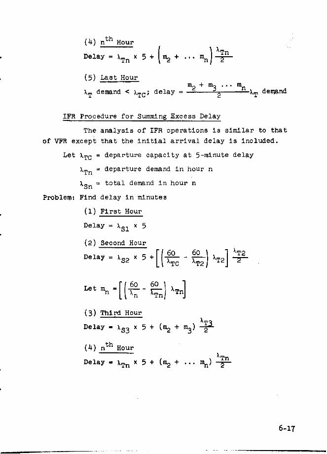
(4) nth Hour%Tn.

Delay = XTn x 5 + (m2 + ... mn)-

(5) Last Hourd2 +m3 ... mn

XT demand < XTC; delay 2 XT demand

IFR Procedure for Summing Excess Delay

The analysis of IFR operations is similar to that

of VFR except that the initial arrival delay is included.

Let XTC = departure capacity at 5-minute delay

XTn = departure demand in hour n

%Sn = total demand in hour n

Problem: Find delay in minutes

(1) First Hour

Delay = XS1 × 5

(2) Second Hour

Delay = S2 X 5 + 6o 6o 2 --2"

kXTC T2

Let mn [(60 60) )Tn]

(3) Third Hour

Delay = xS3 x 5 + (M2 + m3 ) 23

(4) nth HourXTn

Delay lxTn + (m2 + ... m n ) 2

6-17

(5) Last Hourm2 + ...

XT demand < XTC; delay- X2 . T demand

6. ECONOMIC ANALYSIS

The final chapter of the Airport Capacity Handbook

(reference 11) details the procedure to be used for an eco-

nomic analysis of an airport design. This is basically

similar to the technique developed in the previous work.

6-18

TABLE 6-I

T, AVERAGE MINIMUM INTERVAL BETWEEN SUCCESSIVE

DEPARTURES ON SAME RUNWAY (IFR ESTIMATE FOR 1970)

Aircraft Class Aircraft Class T*(Departure) (Departure) (Sec)

A A 68

A B 70

A C 55

A D+E 64

B A 86

B B 60

B C 50

B D+E 45

C A 91

C B 67

C C 52

C D+E 48

D+E A 96

D+E B 90

D+ E C 68D+E D+E 52

*T = average minimum interval between successive departures.

6-19

TABLE 6-1i

F, AVERAGE MINIMUM INTERVAL REQUIRED FOR DEPARTURERELEASE IN FRONT OF AN INCOMING ARRIVAL

(IFR ESTIMATE FOR 1970)

Aircraft Class Aircraft Class F*(Departure) (Arrival) (Sec)

A A 55

A B 64

A C 67

A D 69

A E 73

B A 51

B B 41

B C 43

B D 45

B E 54

C A 55

C B 44

C C 42

C D 39

C E 48

D A 56

D B 50

D C 38

D D 35

D E 39

E A 61

E B 50

E C 48

E D 35

E E 39

*F = average minimum interval required for departure release.

6-20

TABLE 6-111

A, AVERAGE MINIMUM INTERVAL BETWEEN SUCCESSIVE ARRIVALS

ON SAME RUNWAY (IFR ESTIMATE FOR 1970)

Aircraft Aircraft Closest CommonClass Class A* Distance Path Length

(Arrival) (Arrival) (see) (n mi) (n mi

A A 83 3.0 -

A B 86 2.5 8.0

A C 95 2.5 7.0

A D + E 103 2.0 6.0

B A 83 3.0 -

B B 76 2.5 -

B C 79 2.3 7.0

B D + E 91 1.9 6.0

C A 83 3.0 -

C B 76 2.5 -

C C 82 2.3 -

C D + E 88 1.9 6.0

D + E A 83 3.0 -

D +E B 76 2.5 -

D + E C 82 2.3 -

D+E D+E 83 1.9 -

*A = average minimum interval between successive arrivals.

6-21

FIGURE 6-1. INTERSECTING RUNWAY WITH CLOSE INTERSECTIONS

A.

F DATA

STORAGE

CONSTANTS

VF CLULT

INPT: RF

I PUOTA (IM700CMPT R

0

Wz z

4o go o

0 0> 0~oah~ wZ0 w U1

z; N U. x U.

.0 (A u Ez 049 . 4 4W § + w W. . 0wc L z wU IK a 12z5

LL K wz Il0 d 10:CIaZz -

o NP-4 3

cc p. a w w .c

> N

~ H7 - ~ -~--N NNN NN NNN NN 2

r UC 4OQ.-4 N~ Itu .A . o 4* P~00 N at t A U% 0, .0 * -e A

U..

-d~ Nn w (71 012 N~ N 2 4 4 6M rE -P-a m44 % (P( 10p-I-

le LM a 0 0 0 N N m ( AO LA 0 . 0 n- nUN4 -r

0 ~04

--X

m f* -N WNP 00 0 0 0 M .0000 U6 0 0000 000000 0 0 00 0 0 0 00 N

Z 4 0r. AL n ---- c

10

UNV

VII. REFERENCES

1. M. A. Warskow et al., "Airport Runway and Taxiway Design,"Report No. 7601-1, Airborne Instruments Laboratory,July 1960.

2. P. H. Stafford,et al., "Airport Terminal Plan Study,"Report No. 7601-5, Porter and O'Brien and Airborne Instru-ments Laboratory, February 1961.

3. "Runway Characteristics and Performance of Jet Transportsin Routine Operation," Report No. 5791-15, AirborneInstruments Laboratory, March 1960.

4. R. Horonjeff et al., "Exit Taxiway Locations," Instituteof Transportation and Traffic Engineering, University ofCalifornia, September 1960.

5. "Runway Characteristics and Performance of Selected Pro-peller-Driven Aircraft in Routine Operation," ReportNo. 5791-15, Airborne Instruments Laboratory, April 1960.

6. "Airport Design 1961," Airport Engineering Branch, Air-ports Division, Bureau of Facilities and Material, Fed-eral Aviation Agency, 1961.

7. W. J. Offutt, "Study of Mobile Lounge and Other ApronTraffic Delays at Washington Dulles International Airport,"Report No. 7601-2, Airborne Instruments Laboratory, Jan-uary 1961.

8. W. J. Offutt, "Final Report on Study of Mobile Loungeand Other Apron Traffic Delays at Washington DullesInternational Airport," Report No. 7601-3, AirborneInstruments Laboratory, January 1961.

9. E. N. Hooton, "Staging of Runway Construction at NAFEC,Atlantic City, New Jersey," Report No. 7601-4, AirborneInstruments Laboratory, December 1961.

10. M. A. Warskow et al., "Aircraft Runway and Taxiway Design,Excerpts on Typical Configurations, Capacities, Evalu-ation of Design," Report No. 7601-H-l, Airborne Instru-ments Laboratory, July 1960.

11. Airport Capacity, A handbook for analyzing airportdesigns to determine practical movement rates and air-craft operating costs. AIL Report 7601-H-2, June 1963.

7-1

12. Analysis of Capacity and Staging of Runway Constructionat Chicago O'Hare Airport, AIL Report No. 8914-1dated April 1962, and Supplement AIL Report No. 2742-1

dated January 1963.

13. M. A. Warskow, et al., "Airport Facilities for General

Aviation," Report No. 1400-1, Airborne Instruments

Laboratory, Report No. 1400-1, November 1952.

7-2

VIII. CONCLUSIONS

The SAM and FIM mathematical models, together with

the service times observed or interpreted from the field

data, reproduce airport operations in terms of movement rate

versus delay for the following situations:

i. Single, parallel, intersecting, andopen V runway configurations,

2. VFR and/or IFR operations,

3. Runway/taxiway intersection crossings.

The model analysis is based on observed safe

operating practices. Validation testing has shown that the

combined model/input-generation program, measures delay with

sufficient accuracy, and represents safe operations with

sufficient faithfulness to constitute a standard of evalua-

tion for operational performance and airport design.

It is noted that assuming a Poisson arrival input

(the bases for the models) is a desirable public policy

(properly conservative).

Field data has indicated that, for similar runway

configurations, handling similar types of aircraft in VFR,

there is little or no difference between the behavior of

experienced controllers and pilots from one airport to

another, other than very short-term effects. Presumably

this holds in IFR, but here the evidence is not yet as clear.

Because of this conformity, the technique provides a common

national standard for evaluating airport design.

With regard to capacity, airspace restrictions and

limitations have more effect on departures than on arrivals.

The effect on arrivals tends to be more in terms of economics

8-i

than capacity. Iack of airspace routings on depdrtures

requires longer spacing intervals between successive depar-

tures. This, in turn, causes greater departure delays,

which tend to clog the airport. For arrivals, similar air-

space limitations will not necessarily reduce the arrival

rate, but may cause devious routings, off-optimum speeds,

etc., which have economic repercussions.

Airport altitude has little effect on airport

capacity except for increased runway occupancy for landing

aircraft. This effect can be calculated.

Runway occupancy time can now be calculated to a

reasonable degree of accuracy for any given runway/turnoff

configuration. The technique developed should be regarded

as interim since it requires further refinement to provide

information on the use of turnoffs. Use of the technique

has provided some insight into the optimum placing of run-

way turnoffs, and it is considered that some extra work on

this aspect would provide valuable data. The model/input-

generation program can be used to evaluate the effect of

altering runway occupancy times.

The techniques developed and the data accumulated

should have some bearing on the airspace and airport simu-

lation experiments presently being conducted by the FAA.

It has been determined that the steady-state models are

valid in analyzing traffic flows, which vary from hour to

hour provided that certain stated rules of application are

applied. It therefore follows that the techniques would

provide a good starting point on which to base airspace/

airport simulation studies, and the spacing data can be

used directly in the actual simulation.

8-2

- In preparing forecasts for economic analyses of

airports it is necessary to project known figures of airport

movements. At some airports this is very difficult because

present statistics available from the FAA Air Traffic Activ-

ity Reports are sometimes inadequate since helicopter and

training flying (touch-and-go movements) are not separated.

Helicopters very rarely use existing fixed-wing runways, and

though their operations place a load on controllers they do

not impose a runway capacity problem. At some airports

touch-and-go operations (both helicopters and fixed-wing

aircraft) are often performed away from the primary runways

and are counted as two movements (an arrival and a departure).

Again, this may be valid in determining controller work load

but in terms of runway usage it greatly distorts the airport

movements.

Aircraft population greatly affects airport capac-

ity. Present tower statistics are inadequate to accurately

gage whether any one airport is working at or close to capac-

ity.

Since completing the handbook it has become appar-

ent that, spacing intervals of jet aircraft have been some-

what reduced in both VFR and IFR. Also in some instances

there has been local relaxation of rules governing the

operation of intersecting runways.

8-4

IX. RECOMMENDATIONS

The models and parameters input techniques should

be adopted as a standard for evaluating airport design and

as a baseline for future simulation studies. It is recom-

mended for use in evaluating the traffic processing capa-

bility of an operating facility.

There should be periodic reviews and data taking

relevant to the models to periodically amend the handbook

as new aircraft and control techniques are introduced. This

will also update the data library available for simulation

experiments.

A review period of two to three years is suggested

to cover 2 airports for VFR operations, and 2 airports for

IFR operations. These airports should be selected on the

basis of high movement rates and other interesting operating

situations which have developed since the preceding period.

Since data taking on this project ended in early 1962, the

first review should occur during 1964-1965.

Future studies should examine the use of the tech-

niques for applying flow control and further work should be

performed on the economic aspects of airport design and

traffic control techniques.

The question of runway occupancy and placement of

turnoffs should be further investigated:

1. To compile a library of data on aircraftperformance on the runway subject to param-eters such as rain, runway length, posi-tion, and type of turnoffs.

9-1

2. To provide a more accurate and graded (butessentially simple) technique for estimatingrunway time and use of exits.

3. To provide a scientific basis for deter-mining optimum turnoff locations, eitherright-angled exits or high-speed turnoffs..

Aircraft movement statistics taken from control

towers should be modified to separate helicopter and touch-

and-go training operations. This should be done as soon as

possible.

Steps should be initiated to improve the quality

of airport movement statistics by listing operations by

time, class of aircraft, and runway used. It is recognized

that this is more complex than present requirements, and

requires that an improved data recording technique (possibly

semiautomatic) be made available to tower personnel.

9-2

APPENDIX A

TIME-DEPENDENT NONSTATIONARY RUNWAY MODEL

1. ARBITRARY ARRIVAL AND SERVICE-TIME DISTRIBUTIONS

The purpose of this appendix is to show the devel-

opment of a time-dependent scheme for a single-server first-

come-first-served queuing model with arbitrary arrival and

service-time distributions. The output of this model will be

the distribution and moment of delay.

The model. The time axis ( t > 0) is divided into

discrete quantities of equal size At. A single server initi-

ates and terminates service of any customer only at times

t i = At and tT = TAt, where T > i > 0. Customers may arrive

in the time interval t, iAt < t < (i + 1) At. If the system

is empty and the next customer arrives at time t = kAt, his

service will initiate at time ti = kAt and this customer will

be undelayed. Should the customer arrive within the time t,

(k-- 1)At < t < kAt, then he will incur some delay.

We are concerned, basically, with the delay that a

customer might incur. In particular, let us think of a film

that has been exposed at the time iAt, i = 1, 2, 3... If the

viewer thinks of himself as the next customer, then what he

sees will be his delay as a function of time at the time that

he is viewing.

Equations of delay. Essentially, the delay to be

incurred at time (i + 1)At will be the delay that was incurred

at time iAt minus the interval of time At, plus the total serv-

ice of all customers that have arrived in the same interval.

Letting w(n, i) be the probability of delay nAt at time iAt,

a(n), the probability of n arrivals in time At, and s(n) the

A-3

probability that service of a customer is ntt, the equations

of delay are

w(o, i + 1) - a(o) [wl, i) + w(O, i)]

w(i, i + i) - a(o) w(2, i) + a(1) s(i) [w(i, i) + w(O, i)]

w(2, i + 1) - a(0) w(3, 0) + a(l) (6(1) w(2, L) + s(2 ) [r1 . wO .]

+ a(2) ex( 2 ) [W(1, i) + w(O, i)]

where sX(n) is a convolution. Generalizing, let si(n) be the

probability that i customers have a total service of nAt, then

(noting that si(n) = 0 for i > n)

w(n, i + 1) - a(o) w(n + 1, i)

" a(1){F "(K) w(n + 1 - K, ) + al(n) [w(1, i) + w(O, i)

+ a(2) E 2 (K) w(n + 1 - K, i) + 82(n) [w(i, i) + w(O, )k1

+ a(n) P'(n)[W(1' i) + w(O, i

Let

b(n) = Z a(j) sS(n)J=l

b(O) = a(O)Then

W(O. i + 1) - b(o) [W(i. i) + W(o 1i)l

w(n, +1) b(O) w(n+1, + +) + b(n) [w(i. 1) w(O, L)] n > (A-1)

A-2

If we let

wi(t) - E w(n, j) tnn-0

b(t) = X b(ri)t"

the generating function form of equation A-1 is

w+ 1(t) =b(t) [wi(t) - wj(O)] + wi(O) b(O)t (A-2)

For the corresponding cumulative form, let

K=n+l

B(n) = b(K)K=n+l

Gjct) E G(n, i)t'n=o

B(t) = B(n )tnn=O

Then from equation A-2

Gi + l(t) =B(t) + b(t) [ap(t) - a(o)1 (A-3)t

or

A-3

nG(n, i + 1) - B(n) + _, b(K). G(n + 1 - K, i)

(A-4)

Expression A-4 is very useful for computing purposes since

the cumulative form easily lends itself to a truncation cri-

terion.

Moments of delay. By repeated differentiations of

equation A-2, or summing in equation A-i, the first three

moments of delay are

Wl(i + i) =B + Wl (i) - G(O, i)

w 2( +l1) B 2 + W2(i) + 2141(i) ~B1 - 1] + G(0, i) [1l - 2B11

W 3(1 + 1) B + W 3(iL) + 3W2(i) [B1 - 1] + 3W1(i) IB 2 7 2B 1 + 11

- G(O, i) [3BD2 - 3B + 1]

where

Wn(i) = Knw(K, i); B = Knb(n)K=O n K=O

Minimum interval size. The function G(n, i)

G(nAt, iAt) is computed from equation A-4. Experience has

indicated that as At-O, the function G approaches a limit

for each of its arguments. If x = lir nAt, At, At-0; t -

lim iAt, At*0, G(x,t) represents the continuous solution for

x, t > 0. The question of interval size is important in order

to obtain accurate solution at minimal cost, and so, I G(x, t) -

G(nAt, iAtj is small for nAt = x, iAt = t. The recursive scheme

equation A-4 has a very nice criterion.

A-4

Specifically, let b(t) be associated with At, and

F(t) be associated with-L. If b(tm) = (F(t)]m for m > 1,m

then any subdivision of At will not yield greater accuracy in

the function G(x, t) at the corresponding points. Or if b(t)

and E(t) are associated with At, and At/m such that b(tm) =

[F(t)]m; then G(nAt, itt) = G(mn At mi given the same

initial condition. The basic computing difference between

G and G is that the latter requires m time steps of computing,

and the former only one. We shall consider the case of m = 2.

Case 1:

LetGo(t) = 0 = 0o(t)

From equation A-4

Gl(t) 1 - b(t)

whereasG q(t) = 1- S(t)_

_2(t) = t - I(0)(t)] + (t)[(0) -t)t(1 t)

Forming G2 (t) -G l (t2 ), the difference is an odd function

if b(t) = E2(t).

Case 2:

Let

G0 (t) = tn, U 0(t) = t 2 n

G1 - t n - 1 b(t)

1- t

A-5

U2 (t) = 1 - t 2 n - 2 F(t)

1 - t

Again, G2 (t) - Gl(t 2 ) is an odd function if b(t2 ) = g2 (t).

All initial conditions are linear combinations of cases 1 and 2.

In both cases, we have constructed an odd function relating the

function G at two different mesh spacings, one being half of

the other, which is desired. This result leads to a criterion

for minimum interval size.

Moments of b(n). The moments of b can be expressed

in terms of the moments of a(n) and s(n). That is

B 1 = SI1A 1

B2 = S12 (A2 - A,) + S 2 A1

B3 = S13 (A3 - 3A2 + 2AI ) + 3(A2 - A,) SIS2 + AIS3

Steady-state moments of delay. If the steady-state

monents are finite (necessary that B1 < 1), then

lim G(O, i) = G(O) = B S IA1

lBm W+G(o) 1 2B1. - 2(l BI ) -

S12 (A2 - A1) + S2 A1 + S1A 1 (1 - 2S1 A1 )

2(l - SIA,)

A-6

Specifically, let b(t) be associated with At, and

(t) be associated with-A. If b(tm) = [)(t)]m for m > 1,then any subdivision of At will not yield greater accuracy in

the function G(x, t) at the corresponding points. Or if b(t)

and E(t) are associated with At, and At/m such that b(tm)

[S(t)]m; then G(nt, iAt) = G(mn L. mi At) given the samem m

initial condition. The basic computing difference between

G and G is that the latter requires m time steps of computing,

and the former only one. We shall consider the case of m = 2.

Case 1:

Let

G0 (t) = 0 = Go(t)

From equation A-4

Gl(t) 1 b(t)

whereas* 1(t) = i -b(t)

U2 (t) - t[1 - g() +(t)+Et)[(o)- m]2(t) (i - t)

Forming 2 (t) - o1 (t2 ), the difference is an odd function

if b(t2 ) =b2(t).

Case 2:

Let

G0(t) = tn U G0 (t) = t2n

1 - t 1 b(t)

1'') -

1 - t2n-i 1(t)1-t

A- 5

-- o Ct) _1 - t 2 n - 2 y(t)

1 - t

Again, G2 (t) - G1 (t2 ) is an odd function if b(t2 ) = 2(t).

All initial conditions are linear combinations of cases 1 and 2.

In both cases, we have constructed an odd function relating the

function G at two different mesh spacings, one being half of

the other, which is desired. This result leads to a criterion

for minimum interval size.

Moments of b(n). The moments of b can be expressed

in terms of the moments of a(n) and s(n). That is

B1 =SA

B2 = S12 (A2 - A1 ) + S2A1

h3 1S3 (A - 3A2 + 2Al ) + 3(A2 -A l ) SIS 2 + AIS 3

Steady-state moments of delay. If the steady-state

monents are finite (nece. ary that B1 < 1), then

lim G(o, i) = G(0) B B 1 S A1

lim Wl(i) W B2 + G(O) 11 - 2B I,

io= = a 12(1 - BI)

S12 (A 2 - A1 ) + S2A, + SIAl (1 - 2SIA I )

2(1 - S1A,)

A-6

Jim W 1(i) =W = 3W1 [B 2 - 2B 1 + 11 + B a + G(O)[I3B 1 .1 - 3B2]i-*Ce 2 3(1 -B)

Note that the moments are really a summation that approximates,

for the continuous case, an integral. Despite the fact that

G(n, i) may be exact, i.e., At satisfies a minimum criterion,

there is still an error in numerical integration that should

be corrected.

Example 1:

Let

a(n) = e- ,At(XAt)n R(n) = e- , An n !M

s(l6t) = 1 i(2At/2) = 1

At(, - t2 )

b(t) = e -XAt(l-t) b(t) = e

In this case b(t2) = b(t)

Example 2:

For the Poisson distribution,

A1 = %At, A2 = (uAt)2 + (xAt)

A3 = (xAt) 3 + 3(XAt) 2 + At

In the previous considerations, Wn (i) has been expressed in

terms of intervals of At. If we normalize these moments and

the service distribution in terms of'unit space, we find, for

steady state

G(O) = XS 1

A-7

XS2 I S, At

W = -- 2( l - + 2

2 S 2S 3 xS2Lt xS (1 + xS)(At)2

W2 1 )2 3 + +2( - X5 3(1 - Is,) 2(1 - %sI ) 6(1- xs I )

since At*O, W1 and W2 each approach a limit. However, for

any At, there is an error term for each of W1 and W2.

Consider

()-Z (K- 1)nw (n, i)K=I

Then

W1(1) = Wl (i) = G(O, i)

W2 (i) = W2 (i) - 2Wl(i) + G(O, i)

As i4mw, and for normalized units

W 1 W1 - G(O) At

W2 = W - 2W At + G(o)(Lt) 2

thenW! + W1 = S2W1 +W1 ___2

2 2(1 - XS1 )

22

W2 + W s2 Sxs ,Sl(l + xs) 2=+ - 3~- ,+ (At) 2

2 2(1 - XSl) 3(1 - XSl ) 6

A-8

To remove an error term of order At in the moments,

w1(i + 1) = w1(i + i) - i + )2

w2 (. + 1) = w2(1 = 1) - Wl(' + 1)

These corrections can be applied only after the

basic iteration scheme on page A-2 has been applied for all

time steps.

2. POISSON ARRIVAL DISTRIBUTIONS

In the first part of this appendix the theory is

presented for a time-dependent queuing model with arbitrary

arrival and service-time distributions. In this part, the

theory is specialized to a Poisson arrival distribution. In

addition certain details regarding the numerical computation

are given.

Computing procedure for b(n). The b(n) are defined

as

b(n) = a(J) dJ(n) n > o

(A-5)

b(o) = a(o)) n = o

where sJ(n) refers to the jth convolution of the service-time

distribution s(n), and sJ(n) can be interpreted as the prob-

ability that J customers have a total service of nat. Note

that sl(n) = s(n).

A-9

The arrival rate in time At is X, and the Poisson

distribution can be defined as

a(o) =

(A-6)

a(n) = a(n - n > o

Given a prescribed truncation criterion e, define NA as the

smallest integer such that

E a(n) <e

n=NA

Associated with the service-time distribution,

there will be two integers N1 and N2 such that N1 is the

smallest integer for s(n)>o[that is, s(n) = o for n < N]

and N2 is the largest integer for s(n) > o [that is, s(n) =

o for n > N2]. The convolutions of s(n) can then be computed

as

J=min (n, N2 )

sJ(n) = E sJ'l(n - J) s(j) J > 2

J=max (1, N1 ) (A-7)

= o if max (1, N) > min (n, N2 )

Note that si(n) = o for n < iN1 , n > iN2. In the computing

scheme to be described, it is necessary to retain only s(n),s-l(n), si(n); the values of si+l(n) being written over the

values si-l(n). The following is the scheme used in the com-

puter:

A-1O

1. Using equation A-6, compute a(n), o < n < NA

2. Let b(n) = s(n) a(l) N1 < n < N2

= 0 n < NI; n > N2

3. b(o) = a(o)

B(o) = 1 - b(o) [B(n) are cumulative distribution)

4. B(n) = B(n - 1) - b(n) 1 < n < N 1

5. Set i = 2 [$referring to the order of the convo-lution of sl(n), define s1 (n) = s(n)]

6. Using equation A-7, find si(n), iN1 < n < iN 2

7. Let b(n) = a(i) si(n) + b(n), iN 1 < n < N2

8. Let B(n) = B(n - 1) - b(n), (i - 1). N1 + 1 < n < iN19. If B(iN1 ) < c, all of the b(n), B(n) have been defined;

further contributors will be smpll for small e, thendefine NB = iN1 and the routine is finished.

10. If i > NA

B(n) = B(n - 1) - b(n) (i - I) N + 1 < n < iN 2

Define NB as the smallest n such that B(NB) < P.

11. If N cannot be defined by either step 9 or 10,increase i by 1 (i + l--i), and repeat from step 6.

After NB has been defined, the first and second moments

of b(n) are computed. As a check that the distribution of b

has been correctly computed, the first moment B1 can be com-

puted as either

B = xSI where S1 is the average of service

time distributed (A-8)

NB

B 1 = JZo BB(J) (A-9)

We refer to equation A-8 as the predicted value of B1 and to

equation A-9 as the computed value of B1 .

A-11

Computation of delay probability vector. The delay

probability vector G(n, i) is computed in the'cumulative form

and is defined as kliteratlve scheme):

nG(n, i + 1) = B(n) + L b(k) G(n + 1 - k, i)

k-- o

(A-10)

Since the smallest non-zero term in B(n) is B(N b),

the upper limit in the summation in equation A-10O is at most

N b* Further, let L K be defined as the smallest integer such

that G(L K, i) < c. In the summation in equation A-10, n + 1-

j < L K' The delay vector can then be defined as

min (n, NB)

G(n, i + 1) =B(n) + 7b(k) G(n + 1 =k, i)

k--max (o, n+l-L K)

(A-1l)

for max (o, n + 1 - L K).5 mmn (n, NB)

= B(n)

for max (o, n + 1 - L K) > mmn (n, NB)

The first and second moments of G(n, i + 1), Wi (i + i) and

W2 (1. + 1) are defined

w(m + i) = Bi1 + w1(i) -G(o, i) (A-12)

w 2(i +i1) B B2 + w 2(i) + 2Wil(i) [B1 1 ] + G(o, i)[1 =2B,]

(A-13

A-12

As an alternative to equation A-12, the first moment can be

defined as

Wl(i + I) = - a(k, i + 3) (A-14)k-- o

Expression A-12 is referred to as average by iteration, andA-13 as average by summation. Occasionally, these are printed

on line as a check on the work.

It should be noted that expressions A-12 and A-14include an error dependent upon the mesh size. After Wi(i + i)has been computed (for all i), the error can be removed by

defining the first moment.

W1(i + 1) - 0.5 G(o, i + 1)

and for the second moment,

W 2(i + 1) - WI(i + 1) + G(o, i + 1)2

Remembering that arrays in the memory are numberedfrom 1, the computing scheme for equations A-I through A-13

is:

1. Set n = 12. Set temp = B(n) -- in the machine the cumulative

is BB

3. Set k 1 = n + 24. Set k2 = min (NB, kI )

5. Set k3 = max (I, k1 - LK)

6. If k3 > k2 go to step 8, if not, go to step 77. For k 3 < J < k 2 i.e., steps 7(a) and 7(b)

A-13

(a) k4 = k- J

(b) temp = temp + b(j) u(k4 )

8. v(n) = temp

if v(n) < go to step 10, if not go to step 9

9. Repeat steps 2 through 8 for 1 < n < 5000

10. If LK = n find diff = maxlu(J) = v(J)Il j S n

11. Set LK for this vector as n

12. Find from steps 8 and 9, Wl(i + 1) and W2(i + 1)

General discussion. The time axis is divided in

increments of equal size. These increments can be grouped

together so that for each of these groups the arrival rate X

are constant. When the arrival rate and service-time distri-

bution are known, the distributions b(n) and B(n) can be

determined. Within a group of time increments, the delay

vector is computed by Iteration until either (1) the distri-

bution of delay has been computed for each time increment

within a group, or (2) the maximum difference between two

successive vectors (with respect to components) is small,

in which case the steady-state theory applies. After steady

state has been achieved, all successive delay vectors will be

identical (with respect to error criteria).

When the delay vectors have been computed for a

group of increments, either there are more groups or all com-

putation has been done.

Initially, the system is empty, and so the delay

vector is zero.

A-14

APPENDIX B

DETERMINATION OF DELAY USING STEADY-STATE

MODELS IN NONSTATIONARY SITUATIONS

The mathematical models used to determine airport

capacity are steady-state models. They are generally used

to determine an operating rate, which provides a specified

average delay. This operating rate is called the practical

airport capacity.

If the operating rate or demand is known, then the

average delay can be determined. However, the demand is a

variable that changes from hour to hour. This variation in

demand is called the daily distribution of traffic. To accu-

rately determine the total delay experienced throughout a

day, it is necessary to make nonstationary or time-depend-

ent analysis. However, the available time-dependent model

is both clumsy to use and only rigidly valid for the first-

come first-served cases. It was important, therefore, to

develop a means of using the steady-state models to determine

the delay experienced with a particular daily distribution of

traffic demand.

Airport demand is generally forecast first on an

annual basis. The forecast can then be broken down to a peak-

day and peak-hour forecast. This in turn may be refined into

average day peak hour and IFR day peak-hour values, and

finally into daily distributions of traffic by hours. In

airport design, the steady-state models, are used to determine

delay on an hour-by-hour basis for two reasons.

1. Summin the delay. To determine total annualdelay [as is done in benefit/cost analyses),it is necessary to analyze the delay on- anhour-by-hour basis (rather than on the basis

B-1

of one operating rate) for each mode of oper-ation and runway configuration, and then sumthe delay by the day and year. How shouldthis hour-by-hour analysis of delay be accom-plished to make sure it approximates theactual delay which occurs on a nonstationaryor time-dependent basis?

2. Practical capacity compared to peak-hourdemand. How can the operating rate at 4-min-ute delay, which we call the practical air-port capacity for large aircraft, be applied tothe forecast peak-hour demand?

To determine the answer to these questions, we have

investigated an application of a steady-state analysis by

comparing the results obtained to those obtained using a

time-dependent analysis. The answers that we found approxi-

mate the actual situation. Our conclusions are as follows:

1. The summing of delay on a daily and thenannual basis will approximate the actualtime-dependent occurrence of delay if it isdetermined by the steady-state method for2-hour intervals and then summed throughthe day. The 2-hour intervals are chosen,beginning with the pair of consecutive hoursthat have the highest average, and then onworking pairs of hours on both sides of thispeak pair.

2. The proper relationship between the steady-state airport capacity and demand operatingrates will vary with the average delay value,which determines the capacity and is asfollows:

(a) For air-carrier operations where Classes Aand B aircraft are present, so that 3-or 4-minute average delay determinespractical capacity, the average of thetwo consecutive peak hours of demandshould not be greater than the prac-tical capacity operating rate corre-sponding to the 3- or 4-minute delayvalue.

(b) Where only Classes C, D, and E aircraftare in the aircraft population, so thata 2-minute average delay determines prac-tical capacity, the forecast peak-hour

B-2

demand should not be greater than the prac-tical operating rate corresponding to the2-minute delay value.

1. SUMMING THE DELAY

To validate conclusion 1, we have used a time-depend-

ent queuing model with a single-server Poisson arrival distri-

bution and arbitrary serving distribution. An average service

time was specified for each hour of the day, and the delay was

computed at 30-second intervals. The computed delay was

recorded at 5-minute intervals throughout the 24-hour period.

Five 24-hour periods with different demand rates and service

times were examined. The time-dependent model is described

in Appendix A. It is a first-come first-served model and thus

is not directly applicable to the mixed runway analyses we are

examining here (which are solved by application of SAM). How-

ever, it was made comparable by developing service times that

would produce a first-come first-served steady-state curve

equivalent to the SAM steady-state curve.

The delay was also determined for the same five

daily distributions of traffic using the equivalent steady-

state models in three different manners. The analysis of the

delay is made on four bases:

1. The cumulative delay was determined using thetime-dependent model on an hour-by-hour basis.

2. The cumulative delay was determined by takingthe steady-state delay for each hourly demandrate and totaling the steady-state delay onthis basis.

3. The cumulative delay was determined for asteady-state interval of 2 hours, wherein thedemand was averaged for the 2 hours to deter-mine the steady-state delay for that 2-hourperiod.

4. The cumulative delay on a steady-state basiswas determined on a 3-hour interval by takingthe demand for 3 hours, averaging it, andfinding the steady-state delay for this aver-age demand rate.

B-3

On the assumption that the time-dependent models

provided the true measure of delay, which was used as a refer-

ence and the percentage variation of each of these three steady-

state analyses was determined from items 2, 3, and 4. Fig-

ure B-I indicates the results.

The 1-hour interval in Figure B-I generally gave

a delay in excess of the time-dependent delay. The 2-hour

interval provided a total that was relatively close, but

slightly under the time-dependent delay. The 3-hour interval

in all cases gave a relatively low value of total delay.

The five cases shown have a definite trend though

each case has a somewhat different traffic distribution. It

is concluded that the 2-hour interval most accurately approx-

imates the time-dependent solution and will give reasonable

answers if used in any economic analysis. It is important to

repeat that the 2-hour interval should be selected on the basis

of taking the peak hour and the adjoining highest hour as the

first pair and then working in pairs in both directions from

these peak hours.

2. PRACTICAL CAPACITY COMPARED TO PEAK-HOUR DEMAND

Because steady-state analysis indicates longer

delays at the beginning of an interval than would actually

occur, it is important to determine how quickly steady state

is achieved, and consequently how closely the steady-state

capacity analyses relates to a peak-hour demand. Several

runs of the time-dependent model are plotted in Figure B-2.

There are four 2-hour intervals shown wherein the steady-state

delay during the second hour is near 2 minutes. In each case,

the time-dependent delay gradually builds up to the steady-

state delay during a 1-hour interval. In other words, since

the utilization is relatively low at the delay value chosen,

the steady-state condition is achieved during an hour of

B-4

operation. Therefore, for airports where a 2-m[rnute delay

determines the capacity, the forecast demand peak hour should

not be greater than the steady-state forecast operating rate.

Three 3-hour intervals are shown where, at the begin-

ning of the second hour, a 2-hour demand is sufficient to cause

a steady-state delay of about 4 minutes. In each case the

time-dependent delay achieves steady-state before the end

of the first hour. In a typical case (ORD 530/1, the steady-

state delay is 4.0 minutes for 0800 - 0900 but the time-depend-

ent delay at the end of that hour has not attained the steady-

state delay.

Figure B-2 also shows one case (ORD 430/3) where the

steady-state delay starts at 3.4 minutes for 1 hour, goes to

5.1 minutes for the second hour, and 7.5 minutes for the third

hour. In this instance the time-dependent delay never does

achieve steady state, but always lags the steady-state case

and delay, increasing as the steady-state delay increases.

These examples indicate that, at airports where 3

and 4 minutes determine the practical capacity, a 2-hour inter-

val is necessary to achieve steady-state conditions. There-

fore, the method of comparing the peak-forecast demand to the

airport capacity is to take the peak-hour demand and its adja-

cent highest hour, average these two hours, and compare them

with the steady-state capacity. If the demand is not greater

than the airport capacity, the delay will not exceed the speci-

fied 3 or 4 minutes.

B-5

I0

-Ji 8

I-zhi 6z 0

0.

S 4 1-- -HOUR INTERVAL (0)i

2

I- 00

------- - 2-HOUR INTERAL (0)

I-

-1 0

u __ ~ 3-HOUR INTERVAL(0

-12

~ 12

4 -14

FIGURE B-I. COMPARISON OF STEADY-STATE DELAY WITH TIME-DEPENDENT DELAY

1 8~

I-E-4

0U

G3wnl N1 A'1130I NI&IWI AV3O iVOWW OY

t8 t

.- 1. - I -

-~E-4

sunfNim NI Avl3a Ljw3iv 3OVw3AV

SI~flNIA NI AtW130 LAVWOVIV IMMY

APPENDIX C

EFFECTS OF AIRPORT ALTITUDE ON RUNWAY CAPACITYZ

Because airport altitude is known to affect aircraft

landing and takeoff performance, an airport survey was con-

ducted at Stapleton Field, Denver, Colorado (elevation 5331 feet

AMSL) to measure aircraft intervals. The intervals of interest

were the same as those measured at other .airports:

R = Runway occupancy for arrivals

T = Departure-to-Departure interval

A = Arrival-to-Arrival interval

Fmin = Departure followed by arrival

With the exception of R, the time intervals can only

be used for analysis when it is assured that an average minimum

exists (Section IV). Because movement rates per runway were

rather low at Denver (averaging XS = 25), the number of usable

intervals tended to be rather low. However, sufficient data

was gathered to conclude the following:

R = Some increase.

T = Little or no change

A = No change

Fmin = No change

On the basis of aircraft performance it might be

expected that the interval T would increase. At higher alti-

tudes engine thrust and propeller efficiency is reduced, thus

decreasing acceleration and lengthening the takeoff roll.

Some times taken at Denver from start roll to wheels off for

various types of aircraft showed that there was an increase

in this interval of some 6 seconds for Classes A and B aircraft

compared with airports having elevation between 0 and 100 feet

AMSL.

C-1

However, even though this particular effect was meas-

ured, the interval T (which is from start roll of the first

departure to start roll of the second departure) was very sim-

ilar to the data taken at the other airports. Figure C-1 shows

the VFR curve of T versus XS for pairs of Classes D and E aircraft.This cirve is the average value of the data points accumulated

at the other airports. The individual points are those obtained

at Denver.

Similar data was obtained for the interval A, which

is the average minimal interval between successive arrivals at

the runway threshold. An example of the Denver data versus

other airports is presented in Figure C-2.

For all the intervals of T and A, there was some

scatter about the original VFR curves but no significant trend.

Therefore, it was concluded that for a]l practical purposes

aiport altitude had no effect on these intervals.

The same was true for the interval F. Here, the

minimums measured at Denver for different aircraft class combi-

nations showed no definite trend compared with those taken at

other airports. In fact there was a remarkable similarity.

The only definite effect of airport altitude was

apparent in the runway occupancy times. This was somewhat

complicated by the fact that the runways at Denver generally

have rather poor exits. However, despite this, the increased

times were noticeable.

Section IV of this report and Appendix C of the Air-

port Capacity Handbook detail the procedures for determining

altitude effects upon runway occupancy based on aircraft per-

formance and the Denver measurements.

C-2

00

90 T =DEPARTURE /DEPARTURE INTERVALCLASS D/E FOLLOWED BY CLASSD/E ON SAME RUNWAY

80

700

0 70U) s

ui 40 NOMA

30.

20

10S

40

0 302 3 0 o6

TOTAL MOVEMENT RATE~ (X.,)PER HOUR

FIGURE C-1. INTERVALS OF T MEASURED AT DENVER

100I

A ARRIVAL/ARRIVAL INTERVAL90 CLASS C FOLLOWED BY CLASS

so D/E ON SAME RUNWAY

80

5 0 NOMA

zo 4D

(-)

> 00

20

4 10

40

00 10 20 30 40 50 60o

ARRIVAL RATE (,)PER HOUR

FIGURE C-2. INTERVALS OF A MEASURED AT DENVER

APPENDIX D

ANALYSIS OF AIRCRAFT SPEEDS ON APPROACH

The radar photography of the airport surveillance

radar (ASR) scopes taken during the surveys on this project

allowed some analysis of aircraft speeds on approach.

For this analysis, the films from the surveys at

Washington National, Chicago O'Hare, and Idlewild were used.

It was only possible to use data from the days when aircraft

were using the ILS for approach and landing, since this

required pilots to fly a straight-line track. This require-

ment meant that, in general, only IFR days could be analyzed,

and since in IFR conditions the numbers of Classes D and E air-

craft are reduced, most of the speed data could only be

obtained for Classes A, B, and C. (No Class A at Washington.)

Times were measured between the 10- and 5-mile mark-

ers on the radar scope using the clock of the recording system

for this purpose.

The final results are shown in Figure D-1. These

graphs show percentage of each aircraft class versus approach

groundspeed (10-knot increments) for the three airports. Also

shown on each graph is the average speed for that class for

the particular day at the airport.

It should be emphasized that the speeds shown are

groundspeeds, which explains the large variations of the aver-

age speeds betwe2en different days at the three airports. For

example, at Chicago O'Hare on March 6th, the aircraft were

approaching the airport on the ILS in the direction of

140 degrees. The surface wind on that day averaged 250 degrees

25 knots gusting to 40 knots. Therefore, there was a strong

D-1

tailwind component that boosted the average groundspeeds to

174 knots (Class A) and 161 knots (Class B). The more normal

average of groundspeeds for these aircraft in headwinds or

crosswinds is 133 to 150 knots (Class A) and 118 and 139 knots

(Class B). The situation at Chicago O'Hare on March 6th was

somewhat unusual because the aircraft were only using the ILS

for approach and were breaking off at the outer marker to cir-

cle around to runways 22 and 27 for the actual landing.

Since the aircraft were not landing directly from-,.

their ILS approaches, this would probably account for the

higher approach speeds in addition to the wind component facter.

D-2

100

5 MARCH 1961

so _CHICAGO O'HARE

. CLASS A

AVERAGE RUNWAYS 32L AND 32R(138 KNOTS) 2 AIRCRAFT

-60

40-

20

z

90 100 110 120 130 140 150 60 170 ISO 190 200 210APPROACH GROUNOSPEED IN KNOTS

100

5 MARCH 1961so CHICAGO O'HARE

-. 80 CLASS SRUNWAYS 32L AND S2RIS AIRCRAFT

o60 AVERAGE(122 KNOTS)

0S40

0

90 900 110 120 ISO 140 ISO 160 170 Igo ISO 200 210APPROACH GROUNOSPEEO IN KNOTS

FIGURE D-1. AIRCRAFT APPROACH SPEEDS FROM 10 TO 5 MILESSHEET 1 OF 4

100

6 MARCH 1961

s0 _CHICAGO O'HAREI- 80CLASS A

RUNWAY 14Ro ,28 AIRCRAFT

60

AVERAGEo (174 KNOTS)i- 40

20

90 100 110 120 130 140 ISO 160 170 ISO 190 200 210 220

APPROACH GROUNOSPEED IN KNOTS

!O06 MARCH 1961CHICAGO O'HARE

, 80 CLASS B<a RUNWAY 4Ro 28 AIRCRAFT

60

0 AVERAGE

z 40 (161 KNOTS)

IL 20

0

90 100 110 120 130 140 150 160 170 ISO 190 200 210 220

APPROACH GROUNDSPEED IN KNOTS

100

6 MARCH 1961CHICAGO O'HARE

80 CLASS C

RUNWAY 14Ro6 AIRCRAFT

60 AVERAGE

0 (140 KNOTS)

Z 40

w

o. 20

090 100 110 120 130 140 ISO ISO 170 ISO 190 200 210 220

APPROACH GROUNDSPEED IN KNOTS

FIGURE D-1SHEET 2 OF 4

100

31 MARCH 1961

LA. so WASHINGTON NATIONAL-4 CLASS SU RUNWAY 36~ 605O AIRCRAiFT

0I-40

zw AVERAGE

0 (136 KNOTS)

090 S00 110 120 130 140 150- 160 I70 ISO 190 200 210

APPROACH GROUNDSPEED IN KNOTS

100

31 MARCH 1961-___ ____ ___ ____ ___WASHINGTON NATIONAL

4 CLASS Co RUNWAY 36

___________________________10 AIRCRAFT60

LA. AVERAGE0 (135 KNOTS)

40

w 20

LA 090 100 110 120 130 140 I5O I60 170 ISO 19.0 200 210

APPROACH GROUNDSPEED IN KNOTS

100

SO ___________________ AVEAGE 16 FEBRUARY 1961so. (I5O KNOTS)- NEW YORK INTERNATIONAL

9 CLASS ARUNWAY 411

cr60 11_____________I AIRCRAFT

LA.0

i-40z

20

90 100 110 120 130 140 I5O ISO 170 ISO 190 200 210

* APPROACH GROUNDSPEED IN KNOTS

* FIGURE D-1SHEET 3 OF 4

0

IS FEBRUARY 1961

u- sc NEW YORK INTERNATIONALCLASS 8

o RUNWAY 4R

60 .. 10 AIRCRAFT

U. AVERAGEo (139 KNOTS)

402

Lu 20

090 100 110 120 130 140 15O ISO 170 ISO 190 200 210

APPROACH GROUNDSPEED IN KNOTS

10OC

17 FEBRUARY 1961

ec NEW YORK INTERNATIONALCLASS A

o RUNWAY 22L- S _____________AVERAGE 5____ AIRCRAFT

So (133 KNOTS)

0

w

w20C-

90 100 110 120 130 140 150 ISO 170 ISO 19O 200 250

APPROACH GROUNDSPEED IN KNOTS

I0

17 FEBRUARY 1961

00 s NEW YORK INTERNATIONAL4 CLASS SoRUNWAY 22L

6K 0 AVERAGE 12 AIRCRAFT4 (118 KNOTS)

U.0

40 1 -

20

90 500 110 120 130 540 I50 ISO 570 IGO I9O 200 250

APPROACH GROUNDSPEED IN KNOTS

FIGURE D-1SHEET 4 OF 4

APPENDIX E

MATHEMATICAL DESCRIPTION OF MULTI-SERVER QUEUING MODEL

USED TO COMPUTE GATE DELAY

This appendix is concerned with the numerical treat-

ment of a queuing problem that has constant service time and

many servers. It is expected that this treatment will approx-

imate the solution of a problem regarding the number of gates

required to adequately serve the demand by aircraft. Since

this demand fluctuates with respect to time, the desired solu-

tion is essentially time dependent not steady state.

The time axis (t > 0) is divided into equal incre-

ments of size At (ti = iAt). Service is constant and equal

to nAt. We define:

a(k,'i) = Probability of k arrivals (new customers) in time

(i - n) At < t < it

A(k, i) = E a(J, i) = (cumulative) probability of more

J=k+l

than k new customers in customers in time (i - n)

At < t < iAt

p(k, i) = Probability that there are k customers present

(including those being serviced) at time t = itt.

q(k, i) = p(j, i) = (cumulative) probability of moreJ=k+l

E-1

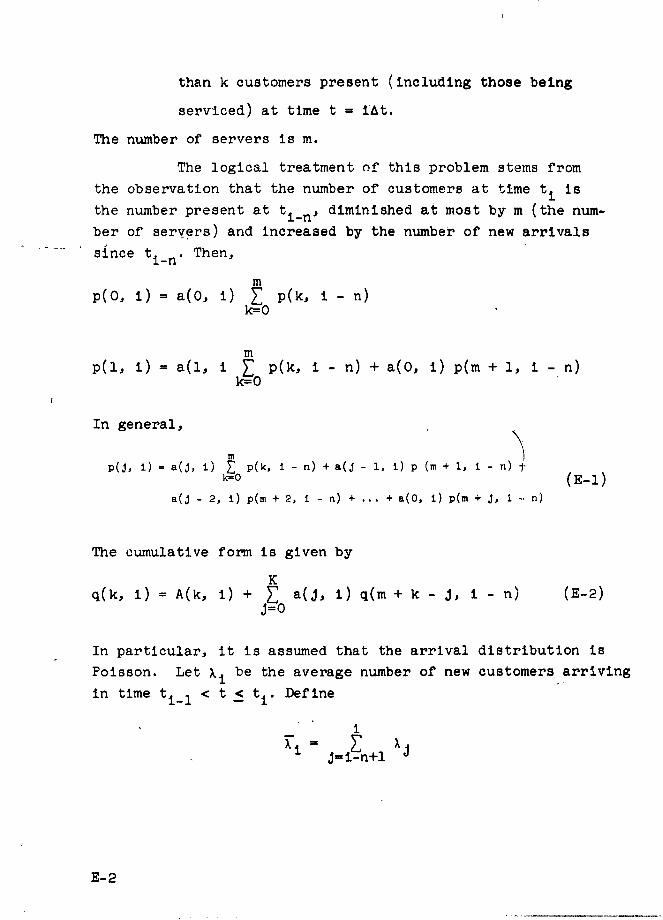
than k customers present (including those being

serviced) at time t = iUt.

The number of servers is m.

The logical treatment of this problem stems from

the observation that the number of customers at time ti is

the number present at tir n , diminished at most by m (the num-

ber of servers) and increased by the number of new arrivals

since tin . Then,

m

p(O, i) = a(O, i) F p(k, i- n)k--O

m

p(l, i) = a(l, i .7 p(k, i - n) + a(O, i) p(m + 1, i - n)k__ 0

In general,

p(j, i) = a(J, i) p(k, i - n) + a(J -i , ±) p (m + 1, i - n) .k=O (E-l)

a(a - 2, 1) p(m + 2, i - n) + ... + a(O, i) p(m + J, i -i n)

The cumulative form is given by

Kq(k, i) = A(k, i) + a(J, i) q(m + k - J, i - n) (E-2)

In particular, it is assumed that the arrival distribution is

Poisson. Let Xi be the average number of new customers arriving

in time ti_1 < t < t . Define

kii

J=i-n+l J

E-2

a(O,.i) = e-T i

a(k, i) =-7i a(k - 1, i) X > 1k

Starting with the boundary conditions:

ki= 0 i<l

p(k, i) = 0 4. < 1 and all k.

Equations E-1 and E-2 are computed successively to maximum

time of interest. Equation E-2 then gives, for each time

interval i, the probability that there are more than k cus-

tomers waiting for gates and being serviced in the gates.

Thus, the probability that all gates are full and no aircraft

is waiting is obtained by k = m.

E-3

APPENDIX F

RINWAY/TAXIWAY CROSSING

The previous report described the use of the Pre-

emptive Poisson Arrivals Model (PAM) for computing delays at

runway/taxiway intersections. The PAM model assumes a Poisson

(random) input for both of two conflicting streams of air-

craft, but one stream of aircraft has complete priority over

the other. The latter is true of a runway/taxiway crossing ........

where the aircraft on the runway (arrivals or departures) have

priority over the taxiing aircraft. However, it has been

determined that it is not correct to assume that both streams

of traffic are Poisson.

In the case of arrivals on a runway, it has been

shown that the original input of arrivals can be assumed to

be Poisson, but that at the runway threshold the arrivals are

necessarily spaced. In other words, the landings on a runway

are the output of a queue. Thus, at the point where the land-

ings and the taxiing aircraft conflict, the landing (arrival)

traffic is spaced.

If we now consider departures (takeoffs) using a

runway conflicting with taxiing aircraft, a similar situation

exists in that takeoffs are spaced--being the output of a queue.

Therefore, if it can be established that the taxiing

aircraft have a Poisson input the conditions are correct for

application of SAM.

For the application of SAM to obtain delay (for

taxiing aircraft) the following inputs apply:

1. Runway Used for Takeoffs Only

XL now becomes XR where XR is the takeoffrate per hour (priority traffic)

F-1

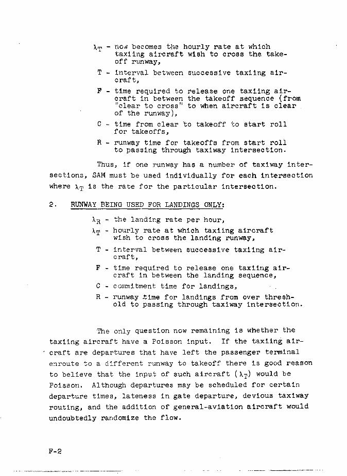
T - novi becomes tlhe hourly rate at whichtaxiing aircraft wish to cross the take-off runway,

T - interval between successive taxiing air-craft,

F - time required to release one taxiing air-craft in between the takeoff sequence (fromclear to cross" to when aircraft is clear

of the runway),C - time from clear to takeoff to start roll

for takeoffs,

R - runway time for takeoffs from start rollto passing through taxiway intersection.

Thus, if one runway has a number of taxiway inter-

sections, SAM must be used individually for each intersection

where XT is the rate for the particular intersection.

2. RUNWAY BEING USED FOR LANDINGS ONLY:

XR - the landing rate per hour,

XT - hourly rate at which taxiing aircraftwish to cross the landing runway,

T - interval between successive taxiing air-craft,

F - time required to release one taxiing air-craft in between the landing sequence,

C - comnitment time for landings,

R - runway time for landings from over thresh-old to passing through taxiway intersection.

The only question now remaining is whether the

taxiing aircraft have a Poisson input. If the taxiing air-

- craft are departures that have left the passenger terminal

enroute to a different runway to takeoff there is good reason

to believe that the input of such aircraft (XT) would be

Poisson. Although departures may be scheduled for certain

departure times, lateness in gate departure, devious taxiway

routing, and the addition of general-aviation aircraft would

undoubtedly randomize the flow.

F-2

If the taxiing aircraft are aircraft that '.Iav;

landed on a different runway, the situation might be sl:ghtly

different. If the problem concerned two close para.lel run-

ways where aircraft that had landed on one runway 1' i.d t.) cross

the other runway, the input of taxiing t ircraft migat nt be

Poisson since the intervals between the landings are not

Poisson.

However, if the runways were Purther apa..t wilh some

taxiway interconnections prior to the cossing, di,.fererc, es in

taxi speeds and path lengths might well 7randomize the derfnd

of the taxiing aircraft.

Also, there is the case of a runway whih is u.0ed

for both takeoffs and landings. In thit case, iriouts 1 ind 2

may be combined by using weighted avera ,es of C and R. Th'us,

the combined landing and tikeoff rateper hour,

XT - hourly rate at which taxi. Ag aircraft wish

to cross the landing/takeorf runway,

T - interval between successive taxiing aircraft,

F - time required to release one taxiing aircraftin between the landing/takaoff sequence.

C - commitment time for landings (multiplied bythe landing probability) plus, caear to take-off to start roll for takeoffs (vultipliedby the takeoff probability).

R - runway time for landings (multiplied bythe landing probability) plus runway timefor takeoffs (multiplied bl' the oakeoffprobability).

In conclusion, it may be stated that a special

application of SAM will allow the computation of taxiway delay

at taxiway/runway intersections for the following cases: (1)

depaitures taxiing across a runway used for takeoffs only,

landings only or both landings and takeoffs; and (2) arrivals

taxiing across a runway used for takeoffs only, landings only

or both landings and takeoffs provided that ;he arrival (taxiing)

input is Poisson.

F-3