Uncertainty (Chapter 13, Russell & Norvig) · CS151, Spring 2005 Modified from slides by David...

CS151, Spring 2005 Modified from slides by David Kriegman, 2001

UncertaintyUncertainty(Chapter 13, Russell &(Chapter 13, Russell & Norvig Norvig))

Introduction to Artificial Intelligence

CS 151

Lecture 1


AdministrationAdministration

• PA 1 will be handed out later this week.

• Programming is in MATLAB - the TA will give aMATLAB tutorial on Thursday.


This LectureThis Lecture

• Probability

• Syntax

• Semantics

• Inference rules

ReadingChapter 13


UncertaintyUncertainty• Let action At = leave for airport t minutes before flight from O’hare• Will At get me there on time?

Problems:1. Partial observability (road state, other drivers' plans, etc.)2. Noisy sensors (traffic reports)3. Uncertainty in action outcomes (flat tire, etc.)4. Immense complexity of modelling and predicting traffic

Hence a purely logical approach either1) risks falsehood: “A135 will get me there on time,” or2) leads to conclusions that are too weak for decision making:

“A135 will get me there on time if there's no accident on I-57and it doesn't rain and my tires remain intact, etc., etc.”

(A1440 might reasonably be said to get me there on time but I'd have to stayovernight in the airport …)


Methods for handling uncertaintyMethods for handling uncertaintyDefault or nonmonotonic logic:

Assume my car does not have a flat tire

Assume A125 works unless contradicted by evidence

Issues: What assumptions are reasonable? How to handle contradiction?

Rules with fudge factors:

A135 ‡ 0 .3 get there on time

Sprinkler ‡ 0.99 WetGrass

WetGrass ‡ 0.7 Rain

Issues: Problems with combination, e.g., Sprinkler causes Rain??

Probability

Given the available evidence,

A135 will get me there on time with probability 0.04

(Fuzzy logic handles degree of truth NOT uncertainty

e.g., WetGrass is true to degree 0.2)


Fuzzy Logic in Real WorldFuzzy Logic in Real World


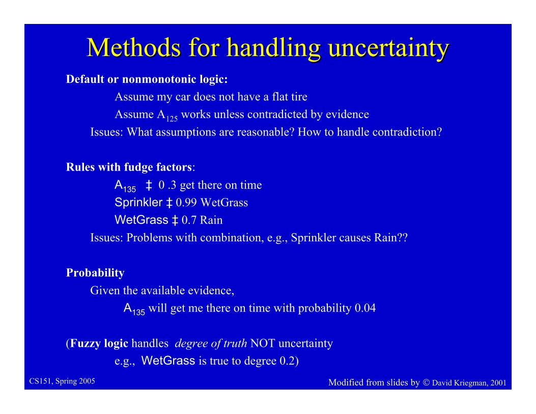
ProbabilityProbabilityProbabilistic assertions summarize effects of

Ignorance: lack of relevant facts, initial conditions, etc.

Laziness: failure to enumerate exceptions, qualifications, etc.

Subjective or Bayesian probability:

Probabilities relate propositions to one's own state of knowledge

e.g., P(A135 | no reported accidents) = 0.06

These are NOT assertions about the world, but represent belief about thewhether the assertion is true.

Probabilities of propositions change with new evidence:

e.g., P(A135 | no reported accidents, 5 a.m.) = 0.15

(Analogous to logical entailment status; I.e., does KB |= α )


Making decisions under uncertaintyMaking decisions under uncertainty• Suppose I believe the following:

P(A 135 gets me there on time | ...) = 0.04




• Which action to choose?

• Depends on my preferences for missing flight vs. airport cuisine, etc.

• Utility theory is used to represent and infer preferences

• Decision theory = utility theory + probability theory


Unconditional ProbabilityUnconditional Probability• Let A be a proposition, P(A) denotes the unconditional

probability that A is true.

• Example: if Male denotes the proposition that a particularperson is male, then P(Male)=0.5 mean that without anyother information, the probability of that person being maleis 0.5 (a 50% chance).

• Alternatively, if a population is sampled, then 50% of thepeople will be male.

• Of course, with additional information (e.g. that the personis a CS151 student), the “posterior probability” will likelybe different.


Axioms of probabilityAxioms of probabilityFor any propositions A, B

1. 0 ≤ P(A) ≤ 1

2. P(True) = 1 and P(False) = 0

3. P(A ∨ B) = P(A) + P(B) - P(A ∧ B)

de Finetti (1931): an agent who bets according to probabilitiesthat violate these axioms can be forced to bet so as to losemoney regardless of outcome.


SyntaxSyntaxSimilar to PROPOSITIONAL LOGIC: possible worlds defined by

assignment of values to random variables.

Note: To make things confusing variables have first letter upper-case, andsymbol values are lower-case

Propositional or Boolean random variables e.g., Cavity (do I have a cavity?)

Include propositional logic expressions

e.g., ¬Burglary ∨ Earthquake

Multivalued random variablese.g., Weather is one of <sunny,rain,cloudy,snow>

Values must be exhaustive and mutually exclusive

A proposition is constructed by assignment of a value:e.g., Weather = sunny; also Cavity = true for clarity


Priors, Distribution, JointPriors, Distribution, JointPrior or unconditional probabilities of propositions

e.g., P(Cavity) =P(Cavity=TRUE)= 0.1P(Weather=sunny) = 0.72

correspond to belief prior to arrival of any (new) evidence

Probability distribution gives probabilities of all possible valuesof the random variable.

Weather is one of <sunny,rain,cloudy,snow> P(Weather) = <0.72, 0.1, 0.08, 0.1>(normalized, i.e., sums to 1)


Joint probability distributionJoint probability distributionJoint probability distribution for a set of variables gives values for each

possible assignment to all the variables

P(Toothache, Cavity) is a 2 by 2 matrix.

NOTE: Elements in table sum to 1 3 independentnumbers.

0.890.01Cavity=false

0.060.04Cavity=true

Toothache = falseToothache=true


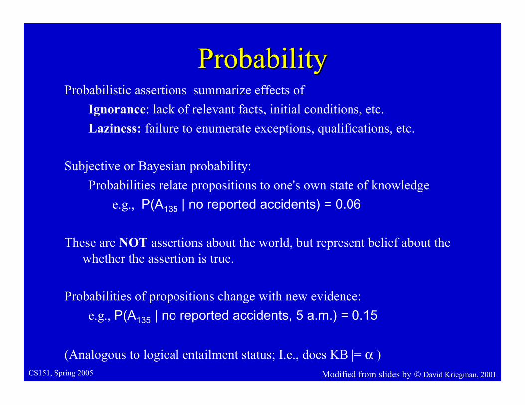
The importance of independenceThe importance of independence

• P(Weather,Cavity) is a 4 by 2 matrix of values:

• But these are independent (usually):– Recall that if X and Y are independent then:– P(X=x,Y=y) = P(X=x)*P(Y=y)

Weather is one of <sunny,rain,cloudy,snow> P(Weather) = <0.72, 0.1, 0.08, 0.1> and P(Cavity) = .1

.09.072.08.648Cavity=False

.01.008.01.072Cavity=True

snowcloudyrainsunnyWeather =


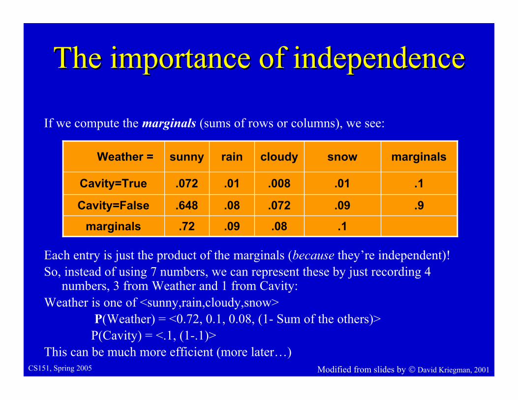
The importance of independenceThe importance of independence

If we compute the marginals (sums of rows or columns), we see:

Each entry is just the product of the marginals (because they’re independent)!So, instead of using 7 numbers, we can represent these by just recording 4

numbers, 3 from Weather and 1 from Cavity:Weather is one of <sunny,rain,cloudy,snow>

P(Weather) = <0.72, 0.1, 0.08, (1- Sum of the others)>P(Cavity) = <.1, (1-.1)>

This can be much more efficient (more later…)

.1

.09

.01

snow

.08.09.72marginals

.9.072.08.648Cavity=False

.1.008.01.072Cavity=True

marginalscloudyrainsunnyWeather =


Conditional ProbabilitiesConditional Probabilities• Conditional or posterior probabilities

e.g., P(Cavity | Toothache) = 0.8

What is the probability of having a cavity given that the patient has atoothache? (as another example: P(Male | CS151Student) = ??

• If we know more, e.g., dental probe catches, then we have

P(Cavity | Toothache, Catch) = .9 (say)

• If we know even more, e.g., Cavity is also given, then we have

P(Cavity | Toothache, Cavity) = 1

Note: the less specific belief remains valid after more evidence arrives, but isnot always useful.

• New evidence may be irrelevant, allowing simplification, e.g.,P(Cavity | Toothache, PadresWin) = P(Cavity | Toothache) = 0.8

(again, this is because Cavities and Baseball are independent


Conditional ProbabilitiesConditional Probabilities• Conditional or posterior probabilities

e.g., P(Cavity | Toothache) = 0.8

What is the probability of having a cavity given that the patienthas a toothache?

• Definition of conditional probability:

P(A|B) = P(A, B) / P(B) if P(B) ≠ 0

P(Cavity|Toothache) = .04/(.04+.01) = 0.8


0.060.04Cavity=true



Conditional probability cont.Conditional probability cont.Definition of conditional probability:

P(A | B) = P(A, B) / P(B) if P(B) ≠ 0

Product rule gives an alternative formulation:

P(A, B) = P(A | B)P(B) = P(B|A)P(A)

Example:

P(Male)= 0.5

P(CS151Student) = 0.0037

P(Male | CS151Student) = 0.9

What is the probability of being a male CS151 student?

P(Male, CS151Student)

= P(Male | CS348Student)P(CS151Student)

= 0.0037 * 0.9 = 0.0033


Conditional probability cont.Conditional probability cont.

A general version holds for whole distributions, e.g., P(Weather,Cavity) = P(Weather|Cavity) P(Cavity)

(View as a 4 X 2 set of equations, not matrix mult.-The book calls this a pointwise product)

The Chain rule is derived by successive application of product rule:P(X1,…Xn) = P(X1, …, Xn-1) P(Xn | X1, …, Xn-1)

= P(X1, …,Xn-2) P(Xn-1| X1 , …,Xn-2) P(Xn | X1, …, Xn-1)= … n= ∏ P(Xi | X1, …, Xi-1) i=1


Bayes Bayes RuleRule From product rule P(A∧ B) = P(A|B)P(B) = P(B|A)P(A), we can

obtain Bayes' rule

Why is this useful???

For assessing diagnostic probability from causal probability:

e.g. Cavities as the cause of toothaches

Sleeping late as the cause for missing class

Meningitis as the cause of a stiff neck

)(

)()|()|(

BP

APABPBAP =

)(

)()|()|(

EffectP

CausePCauseEffectPEffectCauseP =


Bayes Bayes Rule: ExampleRule: Example

Let M be meningitis, S be stiff neck

P(M)=0.0001

P(S)= 0.1

P(S | M) = 0.8

)(

)()||()|(

EffectP

CausePCauseEffectPEffectCauseP =

0008.01.0

0001.08.0

)(

)()|()|( =×==

SP

MPMSPSMP

Note: posterior probability of meningitis still very small!


A generalized A generalized Bayes Bayes RuleRule

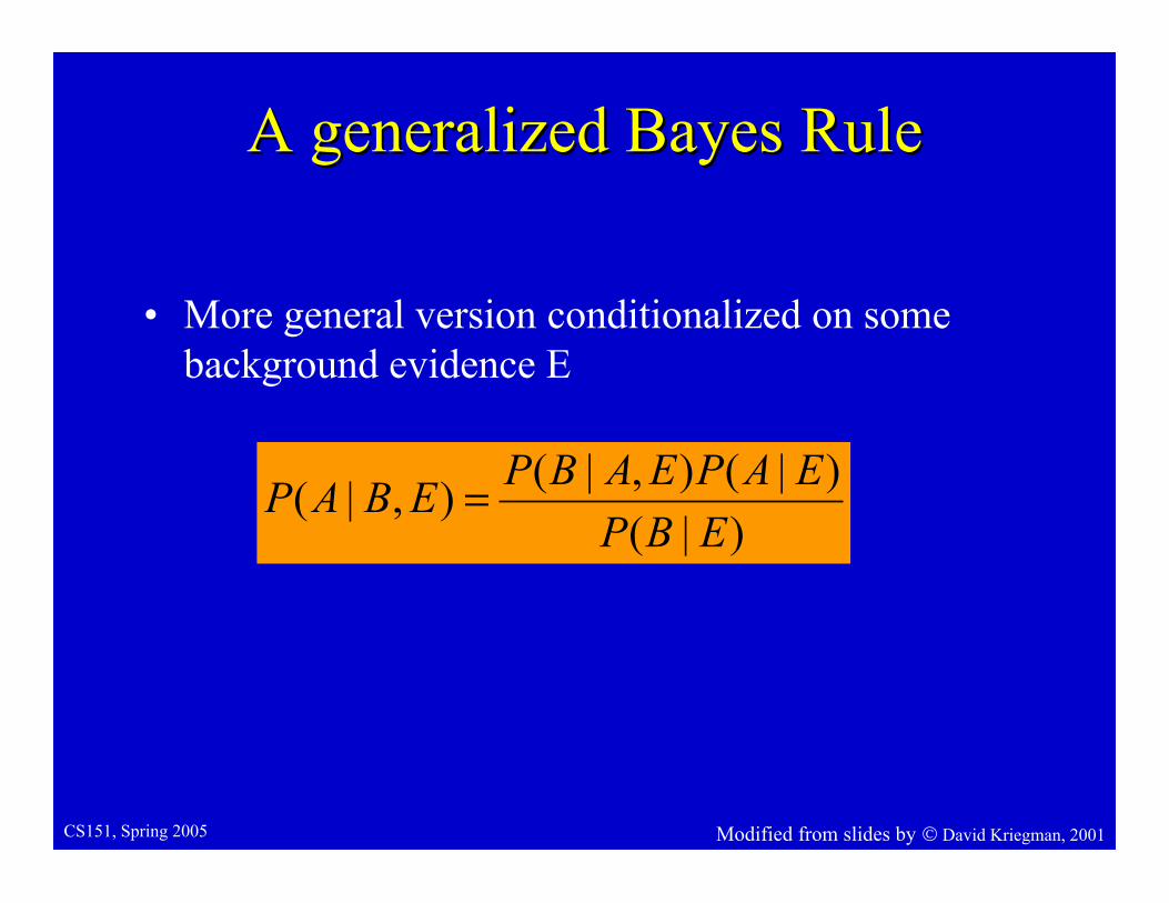
• More general version conditionalized on somebackground evidence E

)|(

)|(),|(),|(

EBP

EAPEABPEBAP =


Full joint distributionsFull joint distributionsA complete probability model specifies every entry in the

joint distribution for all the variables X = X1, ..., Xn

i.e., a probability for each possible world X1= x1, ..., Xn= xn

E.g., suppose Toothache and Cavity are the randomvariables:

Possible worlds are mutually exclusive ‡ P(w1 ∧ w2) = 0

Possible worlds are exhaustive ‡ w1 ∨ … ∨ wn is True

hence Σi P(wi) = 1


0.060.04Cavity=true



Using the full joint distributionUsing the full joint distribution

What is the unconditional probability of having a Cavity?

P(Cavity) = P(Cavity ^ Toothache) + P(Cavity^ ~Toothache)

= 0.04 + 0.06 = 0.1

What is the probability of having either a cavity or a Toothache?

P(Cavity ∨ Toothache)= P(Cavity,Toothache) + P(Cavity, ~Toothache) + P(~Cavity,Toothache)

= 0.04 + 0.06 + 0.01 = 0.11


0.060.04Cavity=true



Using the full joint distributionUsing the full joint distribution

What is the probability of having a cavity given that youalready have a toothache?


0.060.04Cavity=true


8.001.004.0

04.0

)(

)()|( =

+=∧=

ToothacheP

ToothacheCavityPToothacheCavityP


NormalizationNormalizationSuppose we wish to compute a posterior distribution over random variable Agiven B=b, and suppose A has possible values a1... am

We can apply Bayes' rule for each value of A: P(A=a1|B=b) = P(B=b|A=a1)P(A=a1)/P(B=b)

... P(A=am | B=b) = P(B=b|A=am)P(A=am)/P(B=b)

Adding these up, and noting that Σi P(A=ai | B=b) = 1:

P(B=b) = Σi P(B=b|A=ai)P(A=ai)

This is the normalization factor denoted α = 1/P(B=b):

P(A | B=b) = α P(B=b | A)P(A)

Typically compute an unnormalized distribution, normalize at ende.g., suppose P(B=b | A)P(A) = <0.4,0.2,0.2>

then P(A|B=b) = α <0.4,0.2,0.2>

= <0.4,0.2,0.2> / (0.4+0.2+0.2) = <0.5,0.25,0.25>


MarginalizationMarginalization

Given a conditional distribution P(X | Z), we can create theunconditional distribution P(X) by marginalization:

P(X) = Σz P(X | Z=z) P(Z=z) = Σz P(X, Z=z)

In general, given a joint distribution over a set of variables,the distribution over any subset (called a marginaldistribution for historical reasons) can be calculated bysumming out the other variables.


Absolute IndependenceAbsolute Independence• Two random variables A and B are (absolutely) independent iff

P(A, B) = P(A)P(B)

• Using product rule for A & B independent, we can show:P(A, B) = P(A | B)P(B) = P(A)P(B)Therefore P(A | B) = P(A)

• If n Boolean variables are independent, the full joint is:

P(X1, …, Xn) = Πi P(Xi)

Full joint is generally specified by 2n - 1 numbers, but when independent only nnumbers are needed.

• Absolute independence is a very strong requirement, seldom met!!


ConditionalConditional IndependenceIndependence• Some evidence may be irrelevant, allowing simplification, e.g.,

P(Cavity | Toothache, PadresWin) = P(Cavity | Toothache) = 0.8

• This property is known as Conditional Independence and can be expressed as:

P(X | Y, Z) = P(X | Z)

which says that X and Y independent given Z.

• If I have a cavity, the probability that thedentist’s probe catches in it doesn'tdepend on whether I have a toothache:

1. P(Catch | Toothache, Cavity) = P(Catch | Cavity)

i.e., Catch is conditionally independent of Toothache given Cavity

This doesn’t say anything about P(Catch|Toothache)

The same independence holds if I haven't got a cavity:

2. P(Catch | Toothache, ~Cavity) = P(Catch | ~Cavity)


Using Conditional IndependenceUsing Conditional Independence

Full joint distribution can now be written as

P(Toothache,Catch,Cavity)

= (Toothache,Catch | Cavity) P(Cavity)

= P(Toothache | Cavity)P(Catch | Cavity)P(Cavity) (from 1.b)

Specified by: 2 + 2 + 1 = 5 independent numbers

Compared to 7 for general joint

or 3 for unconditionally indpendent.


Belief (Belief (BayesBayes) networks) networks

A simple, graphical notation for conditional independenceassertions and hence for compact specification of full jointdistributions.

Syntax: 1. a set of nodes, one per random variable 2. links mean parent “directly influences” child 3. a directed, acyclic graph 4. a conditional distribution (a table) for each node given

its parents: P(Xi | Parents(Xi))

In the simplest case, conditional distribution represented as aconditional probability table (CPT)


A two node net &A two node net &Conditional Conditional probability tableprobability table

• Node A is independent of Node B, so it isdescribed by an unconditional probability P(A)

• P(¬A) is given by 1 - P(A)

• Node B is conditionally dependent on A. It isdescribed by four numbers, P(B | A), P(B | ¬ A),P(¬B | A) and P(¬B | ¬A).

• This can be expressed as 2 by 2 conditionalprobability table (CPT).

• But P(¬B | A) = 1 – P(B | A) andP(¬B | ¬A) = 1 - P(B | ¬A) .

• Therefore, only two independent numbers in CPT

A

B


ExampleExampleI'm at work, neighbor John calls to say my alarm is ringing, but

neighbor Mary doesn't call. Sometimes it's set off by minorearthquakes. Is there a burglar?

Variables: Burglar, Earthquake, Alarm, JohnCalls, MaryCalls

Network topology reflects ``causal'' knowledge:

Uncertainty (Chapter 13, Russell & Norvig) · CS151, Spring 2005 Modified from slides by David...

Documents

Transcript of Uncertainty (Chapter 13, Russell & Norvig) · CS151, Spring 2005 Modified from slides by David...