Introduction 

Sanger  sequencing  revolutionized  biological  and  medical  research  and  next‐generation sequencing is revolutionizing it again. A single biological sample, that is 

sequenced by  a next‐generation  sequencing platform,  such  as  SOLiD,  produces 30 million  oligonucleotides  or  reads.  But  to  make  sequencing  efficient,  dozens  of 

samples  are  sequenced  simultaneously,  producing  over  a  billion  reads  in  a  single 

run of the sequencing equipment. Thus, two questions arise: One is how to store all the data and the other is what to do with all the data? How to store all the data is a 

problem that  is being  tackled by  those who host  large computer clusters, whether 

stationary or in a cloud. Yet analyzing the millions of reads and designing state‐of‐the‐art  bioinformatics  tools with which  to  analyze  these  data  is  becoming  quite  a 

challenge  for bioinformaticists,  clinicians and biologists alike. For  instance, who  is asking what  biological  and  clinical  questions  and who  is  answering  them  creates 

new roles for researchers. 

 

For my rotation project,  I built a website and analyzed data  that began to address 

these issues. The website uploaded SOLiD sequencer read files associated with the 

picoeukaryote organism micromonas, strain RCC299 and a reference genome for the 

organism and analyzed the data for a given number of samples. I used the unmasked 

reference  assembly  genome  from  the  Department  of  Energy’s  Joint  Genome Institute.  The  RCC299  strain’s  genome  has  17  chromosomes  plus  a  chloroplast 

chromosome.  I  analyzed  the  reads  corresponding  to  the  17  chromosomes.  The 

envisioned output on the website was a multi‐read visualizer of  the 24 samples of 

micromonas.  

 Materials and Methods 

I established a pipeline of computer programs in order to derive the results. Figure 

1 illustrates this pipeline. A suite of software programs created by others was also used  to  derive  the  results.  The  first  software  program  used  was  BWA  (Barrows‐

Wheeler  Alignment),  a  program  that  came  from  the  James  Durbin  laboratory, 

Cambridge University, UK. This “short read alignment to a large reference genome” 

program  allowed  for  mismatches  and  gaps  [Li,  2009].  Bowtie,  produced  by  S. 

Salzberg’s group at the University of Maryland, was another software program that was  used  to map  the  SOLiD  reads  to  a  reference  genome  [Langmead,  2009].  One 

shortcoming  with  both  BWA  and  Bowtie  that  they  did  not  report  all  reads: 

“Whenever bowtie  reports a  subset of  the valid alignments  that exist,  it makes an effort  to  sample  them  randomly”  (Bowtie  manual,  [Langmead,  2009]).  In  other 

words, while BWA simply reports only the first read that maps to a specific genomic position, throwing away the other reads, Bowtie randomly selects one read among 

all  reads  that map  to  a  specific  genomic  position.  There  are  options,  however,  to 

have Bowtie report aligned reads but this subset of reads does not have the genomic position  given  with  them.  The  final  mapping  software  tool  to  be  used  was  Bfast, 

produced at UC Los Angeles, CA in the laboratory of Stanley Nelson [Homer, 2009]. 

Bfast output contained all reads, mapped or not.   

 

The  other  software  tools  that  were  used  were  SamTools,  a  set  of  tools  used  to 

analyze  reads  that  have  been mapped  to  a  reference  genome,  BEDTools,  a  set  of tools also used to produce analyses of reads that have a been mapped to a reference 

genome,  and  PicardTools,  a  set  of  tools  that  change  the  file  format  of  read  files, among other possibilities.  

 

  Figure  1.  Flowchart  of methodology  for  analysis  of  reads:  The  pre‐filter  steps  are 

applied  sequentially  to  raw  reads.  The  pre‐filtering  technique  applied  to  the  raw 

reads  resulted  in  a  very  high  quality  set  of  reads  that  were  then  mapped  to  the reference  genome  of  micromonas.  The  mapping  steps  applied  to  the  pre‐filtered 

reads  resulted  in  a  careful  read  count  for  exons,  introns,  intergenic  regions  and rRNA, along with unmapped reads. 

 

I wrote a number of software programs in order to filter and prepare read files for their analysis. The reads were pre‐filtered before mapping  to a reference genome. 

First, I removed reads with more than one ‘wildcard’ position. That meant that if a 

read had an unknown value at any base,  that read was discarded. Next, a  ‘floating 

window’ was prepared to assess  the quality values  in each read.  If  in a window of 

five  reads,  the  quality  values  for  each  read  averaged  to  10  or  less,  that  read was trimmed at the base. Thus low quality reads were trimmed. Next the P2 adapter was 

matched against each read to see if any of the reads had P2 adapter bases. If so, that 

read was removed. Lastly, if a read was 35 bases or less, that read was discarded. 

 

Next,  the  set  of  filtered  reads  for  each  sample was  converted  from  two  files  (the colorspace  file  and  the  quality  values  file)  into  a  single  file with  fastq  file  format. 

Then, the reads were mapped to a set of poly‐T, C, G, A reads and all SOLiD adapters. If a read mapped to this set, it was discarded. The reads were then mapped to a set 

of  rRNA  for  the  micromonas.  The  reads  that  mapped  to  the  set  of  rRNA  were 

counted and then removed from the larger set of reads. Finally, BWA/Bowtie/Bfast was applied to the set of reads in order to map them to the micromonas genome. I 

used BWA to map the reads of all 24 samples to the micromonas genome. Finding 

that  these  results  were  unsatisfactory,  I  used  Bowtie  and  Bfast  to  map  to  the micromonas genome. For BWA,  the output was a  set of mapped  reads  in SAM  file 

format.  I  converted  the  SAM  files  to  BAM  files  using  the  SamTools  and  then converted BAM  files  to BED  files  using  the BEDTools.  For Bfast  output,  I  had  two 

sets:  One  with  mapped  reads  and  one  with  non‐mapped  reads.  For  the  set  of 

unmapped reads, the output file format was in BAF file format. I used one tool from 

the suite of Bfast tools to convert the BAF file format to SAM file format. I then used 

a tool from PicardTools to convert the SAM file to a fastq file format. This fastq file of 

unmapped reads was mapped against the micromonas genome for the second time 

and the output was used for counting mapped reads and unmapped reads. I fed the 

set of second unmapped reads into Bfast for a third time and used those counts of mapped and unmapped reads. The Bfast mapped reads were in SAM format. Using 

the  suite  of  tools  from  SamTools  and  BEDTools,  the  Bfast  mapped  reads  were 

converted to BAM and then BED file format for each sample.  

 

For  the  BWA  set  of mapped  reads,  I  was  able  to  use  the  BEDTools  software  tool “intersectBed” which  examines  two  files  and  determines  the  intersection  of  those 

two  files  and  counts  the number  of  times  a  read  from one  set  intersects with  the 

second set. A BED file is a collection of genomic positions. Thus each mapped read in each  sample  was  converted  into  genomic  coordinates.  Next,  I  downloaded  each 

chromosome  GenBank  file  for  micromonas.  I  created  a  set  of  all  exons  from  the 

GenBank  file  of  CDS  coordinates  for  micromonas  exons,  by  writing  a  computer 

program  that  isolated each exon’s  start and stop genomic position and converting 

that into a BED file. Then, I intersected the BED file of mapped reads with the BED file of exons to get a count of number of reads which intersected with micromonas 

exons. This means  that  I  counted  the number of  reads which overlapped with  the 

exon genomic regions in the micromonas genome.  

To  create  a  set  of micromonas  introns,  I  used  the  GenBank  files  again.  I  wrote  a program  that  found  the  set of  introns associated  to a genomic  consecutive pair of 

exons in each gene in each chromosome. I intersected the set of introns with the set 

of mapped reads and recorded the counts. I used the GenBank files to create a set of intergenic  regions  for  the  BWA  mapped  reads.  However,  after  discussion  with 

Marcus Breese from Indiana University, I decided that the counts for the intergenic 

regions  were  those  counts  of  mapped  reads  that  remained  after  subtracting  the counts  for  the  exons  and  the  introns.  This  technique  I  used  for  the Bfast mapped 

reads. I was able to compute the exons and introns for each Bfast file for seven of the 

samples  (See  Figure  3).  I  also  mapped  the  total  reads  against  the  chloroplast 

genome of micromonas as well as the genome of another strain of micromonas and the E. Coli genome in order to test for contamination.  

 To create Figures 4 – 28, I wrote a computer program that counted the number of 

mapped  reads at  a  given base  for a  specified  chromosome of  a  reference genome. 

The  program’s  output was  the  number  of  counts  of mapped  reads  and  the  given genomic position of the base. Only nonzero counts were outputted. I created Figures 

2 – 28 using the R graphics package.  

 Additionally,  I  built  a website,  http://inspired.soe.ucsc.edu,  in which  a  user  could 

perform  the  above  calculations  for  SOLiD  reads  for  the  micromonas  organism, namely, mapping SOLiD reads to a reference genome and additionally output those 

reads  in  an  R  software  program  computed  graph  which  plotted  counts  against 

genomic  coordinates  for  the  mapped  reads.  The  user  simply  uploaded  files  of 

colorspace data along with quality values for each read from the SOLiD sequencer, 

along  with  an  uploaded  reference  genome.  The  analysis  was  created  through  a 

series  of  webpages  that  allowed  the  user  to  choose  which  mapping  tool  to  a 

reference genome  they wanted  to use and what  they wanted  to do once  they had 

mapped the SOLiD reads. The R software package was linked to the website so that the graphs could be produced.  

 

Results and Discussion 

I produced a website which could analyze and display the samples. Figures 2 – 28 

were produced on a Mac computer. Figure 4 was partially produced after a number of  attempts:  The Mac  computer  froze  and  the  figure  crashed midway  through  the 

figure’s  production.  Thus  a  snapshot  of  the  figure  was  taken  before  the  figure 

crashed.   

The  goal  of  the  project  was  to  create  a  visualization  tool  for  viewing  the 

micromonas’  samples.  The  resulting  Figures  2  –  3  were  created  to  show  the 

percentage  of  exons,  introns,  rRNA,  intergenic  regions  and  unmapped  rRNA 

computed using the SOLiD data of micromonas. Figures 4 – 28 were created in order to  show  how  the website’s  viewer  looked when  the  data was  analyzed  using  the 

website. The idea was that the user could click on which samples to display or have 

all  the  samples  display.  Figures  4  –  28  are  known  as  “bedgraphs,”  nomenclature used in discussions of the UCSC genome browser. Viewing the Figures 4 – 28 is most 

interesting. The reader can see  that  the genomic patterns change according  to  the sample  displayed.  It  is  clear  that  there  are  different  conditions  that  the  organism 

underwent to create these diverse patterns. 

 Another  useful  visualization  was  “pileups,”  namely  displaying  reads  against  the 

genome. Since the resulting analysis of  the data produced files  in Bed formats,  the 

files could in theory be visualized using the micromonas browser. However after a discussion with  Larry Meyer,  of  UC  Santa  Cruz,  it was  determined  that  these  Bed 

formatted  files  would  overload  the  micromonas  browser  as  well  as  the  UCSC 

browser  (if  the  UCSC  browser  contained  a  reference  genome  for micromonas).  A 

Bed  formatted  file  had  annotations  for  each  genomic  region  that  results  from  the analysis.  It would be possible to place  in the annotation the number of reads for a 

given genomic region, thus permitting a type of pileup. This remains future work for the website.  

 

One crucial point for the analysis of the SOLiD data: I will use the A15_01 sample to illustrate  the  point.  The  total  number  of  raw  reads  is  12,422,404.  After  the  pre‐

filtering, the number of reads was 9,400,465. Bfast mapped 3,936,114 reads to the 

micromonas  reference  genome.  After  running  through  Bfast  twice,  a  total  of 3,938,207  reads  were  produced.  However,  the  preliminary  Bed  formatted  file 

contained only 700,606 unique genomic  regions or mapped reads  (prior  to use of the intersectBed program). Thus, a number of mapped reads was not being counted 

or were being combined to create unique reads. I could have adjusted the number of 

exons,  introns,  rRNA  and  intergenic  regions  by  multiplying  the  numbers  by  a 

common factor of 3938207/700606. This would assume a uniform distribution for 

each  reported  read.  That  is,  each  mapped  read  could  be  assumed  to  have 

approximately 5.5 copies of that identical read. Doing the multiplication, the number 

of exons (876,813 x 5.5) equaled 4,822,471, which was greater than the 3,938,207 

mapped reads. Thus,  there was a non‐uniform distribution of  reads. The best way around this problem would be to map the pre‐filtered reads against the set of exons 

(and, also introns) rather than the whole genome in order to get an accurate count 

of the exon (and introns) reads.  

 

Bfast  worked  in  the  following  way.  It  identified  CALs  or  candidate  alignment locations, known as genomic regions in our nomenclature, for each read. If no CAL 

was  found  for  a  read  then  that  read  was  unmapped.  Another  issue  was  the 

possibility that some unmapped reads may have been copies of mapped reads.  

 

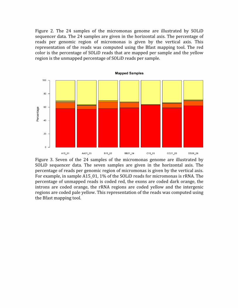
Figure  2.  The  24  samples  of  the  micromonas  genome  are  illustrated  by  SOLiD 

sequencer data. The 24 samples are given in the horizontal axis. The percentage of reads  per  genomic  region  of  micromonas  is  given  by  the  vertical  axis.  This 

representation  of  the  reads was  computed  using  the  Bfast mapping  tool.  The  red color is the percentage of SOLiD reads that are mapped per sample and the yellow 

region is the unmapped percentage of SOLiD reads per sample.  

 

 Figure  3.  Seven  of  the  24  samples  of  the  micromonas  genome  are  illustrated  by SOLiD  sequencer  data.  The  seven  samples  are  given  in  the  horizontal  axis.  The 

percentage of reads per genomic region of micromonas is given by the vertical axis. 

For example, in sample A15_01, 1% of the SOLiD reads for micromonas is rRNA. The percentage of unmapped reads  is coded red,  the exons are coded dark orange,  the 

introns  are  coded  orange,  the  rRNA  regions  are  coded  yellow  and  the  intergenic 

regions are coded pale yellow. This representation of the reads was computed using 

the Bfast mapping tool.  

 

 

 

   

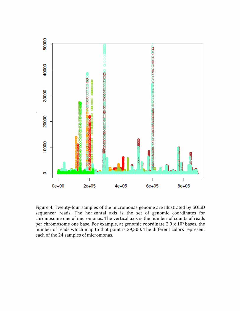
Figure 4. Twenty‐four samples of the micromonas genome are illustrated by SOLiD 

sequencer  reads.  The  horizontal  axis  is  the  set  of  genomic  coordinates  for chromosome one of micromonas. The vertical axis is the number of counts of reads 

per chromosome one base. For example, at genomic coordinate 2.0 x 105 bases, the number of reads which map to that point  is 39,500. The different colors represent 

each of the 24 samples of micromonas.  

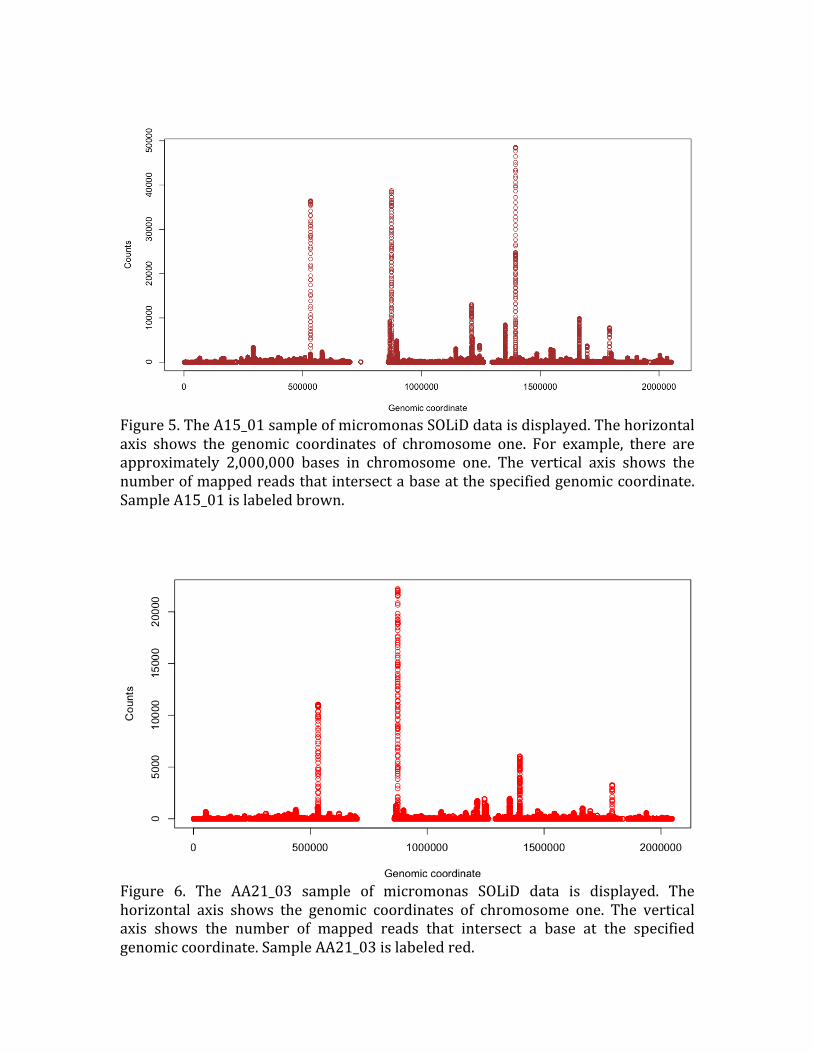
 Figure 5. The A15_01 sample of micromonas SOLiD data is displayed. The horizontal 

axis  shows  the  genomic  coordinates  of  chromosome  one.  For  example,  there  are 

approximately  2,000,000  bases  in  chromosome  one.  The  vertical  axis  shows  the 

number of mapped reads that intersect a base at the specified genomic coordinate. 

Sample A15_01 is labeled brown.   

 Figure  6.  The  AA21_03  sample  of  micromonas  SOLiD  data  is  displayed.  The 

horizontal  axis  shows  the  genomic  coordinates  of  chromosome  one.  The  vertical axis  shows  the  number  of  mapped  reads  that  intersect  a  base  at  the  specified 

genomic coordinate. Sample AA21_03 is labeled red. 

 Figure 7. The B15_02 sample of micromonas SOLiD data is displayed. The horizontal 

axis shows the genomic coordinates of chromosome one. The vertical axis shows the 

number of mapped reads that intersect a base at the specified genomic coordinate. 

Sample B15_02 is labeled orange. 

 

 Figure  8.  The  BB21_04  sample  of  micromonas  SOLiD  data  is  displayed.  The 

horizontal  axis  shows  the  genomic  coordinates  of  chromosome  one.  The  vertical 

axis  shows  the  number  of  mapped  reads  that  intersect  a  base  at  the  specified genomic coordinate. Sample BB21_04 is labeled yellow‐green. 

 Figure 9. The C15_03 sample of micromonas SOLiD data is displayed. The horizontal 

axis shows the genomic coordinates of chromosome one. The vertical axis shows the 

number of mapped reads that intersect a base at the specified genomic coordinate. 

Sample C15_03 is labeled aquamarine.  

 Figure  10.  The  CC21_05  sample  of  micromonas  SOLiD  data  is  displayed.  The horizontal  axis  shows  the  genomic  coordinates  of  chromosome  one.  The  vertical 

axis  shows  the  number  of  mapped  reads  that  intersect  a  base  at  the  specified 

genomic coordinate. Sample CC21_05 is labeled green.  

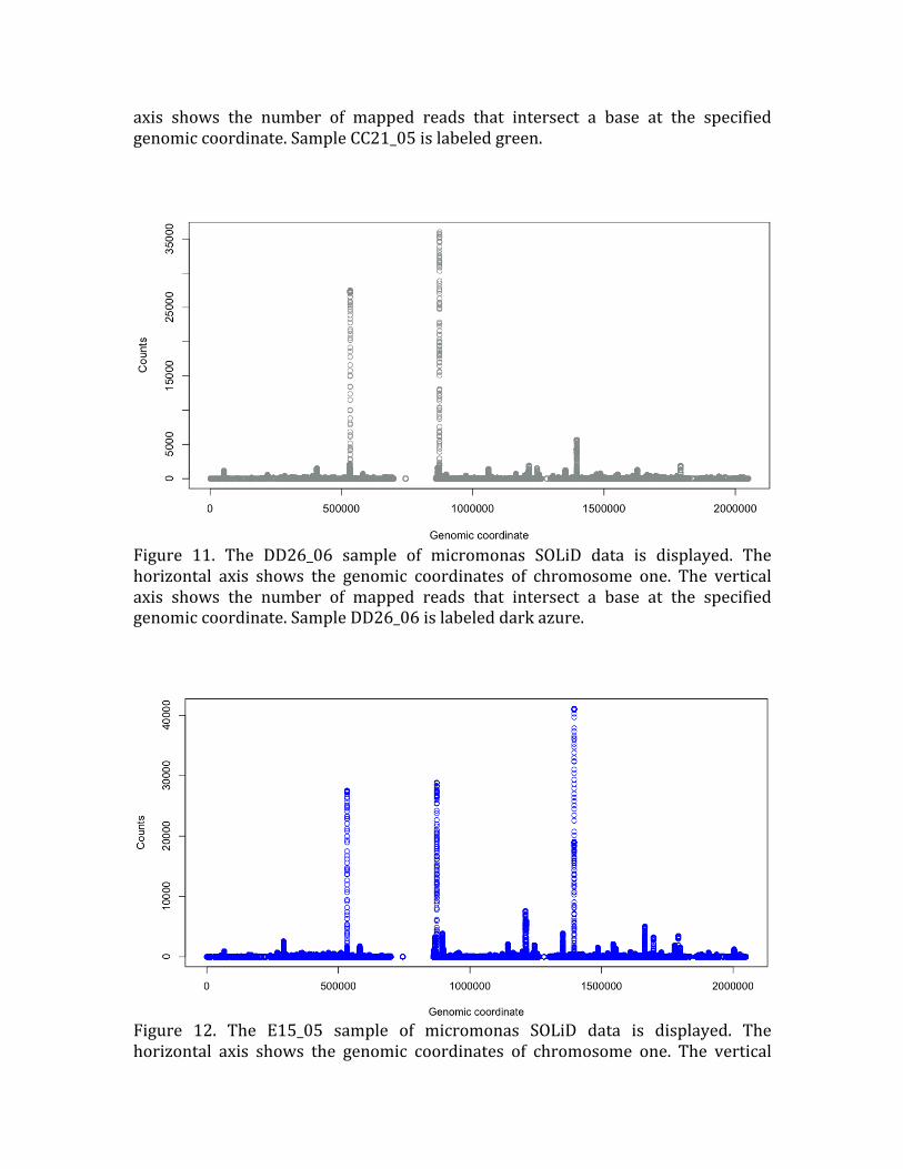
 Figure  11.  The  DD26_06  sample  of  micromonas  SOLiD  data  is  displayed.  The 

horizontal  axis  shows  the  genomic  coordinates  of  chromosome  one.  The  vertical 

axis  shows  the  number  of  mapped  reads  that  intersect  a  base  at  the  specified genomic coordinate. Sample DD26_06 is labeled dark azure. 

 

 Figure  12.  The  E15_05  sample  of  micromonas  SOLiD  data  is  displayed.  The 

horizontal  axis  shows  the  genomic  coordinates  of  chromosome  one.  The  vertical 

axis  shows  the  number  of  mapped  reads  that  intersect  a  base  at  the  specified 

genomic coordinate. Sample E15_05 is labeled blue.  

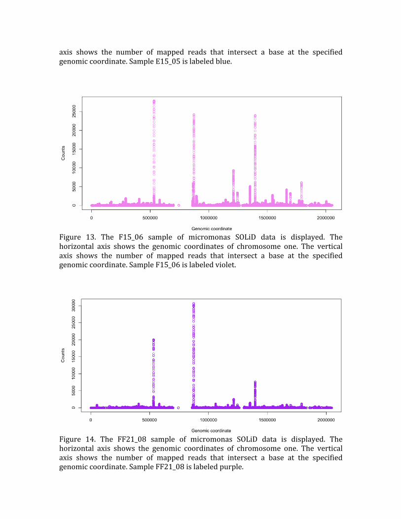
 Figure  13.  The  F15_06  sample  of  micromonas  SOLiD  data  is  displayed.  The 

horizontal  axis  shows  the  genomic  coordinates  of  chromosome  one.  The  vertical 

axis  shows  the  number  of  mapped  reads  that  intersect  a  base  at  the  specified 

genomic coordinate. Sample F15_06 is labeled violet. 

 

 Figure  14.  The  FF21_08  sample  of  micromonas  SOLiD  data  is  displayed.  The 

horizontal  axis  shows  the  genomic  coordinates  of  chromosome  one.  The  vertical 

axis  shows  the  number  of  mapped  reads  that  intersect  a  base  at  the  specified genomic coordinate. Sample FF21_08 is labeled purple. 

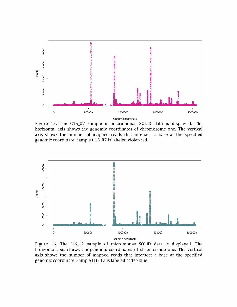
 Figure  15.  The  G15_07  sample  of  micromonas  SOLiD  data  is  displayed.  The 

horizontal  axis  shows  the  genomic  coordinates  of  chromosome  one.  The  vertical 

axis  shows  the  number  of  mapped  reads  that  intersect  a  base  at  the  specified 

genomic coordinate. Sample G15_07 is labeled violet‐red.  

 Figure  16.  The  I16_12  sample  of  micromonas  SOLiD  data  is  displayed.  The 

horizontal  axis  shows  the  genomic  coordinates  of  chromosome  one.  The  vertical axis  shows  the  number  of  mapped  reads  that  intersect  a  base  at  the  specified 

genomic coordinate. Sample I16_12 is labeled cadet‐blue.  

  

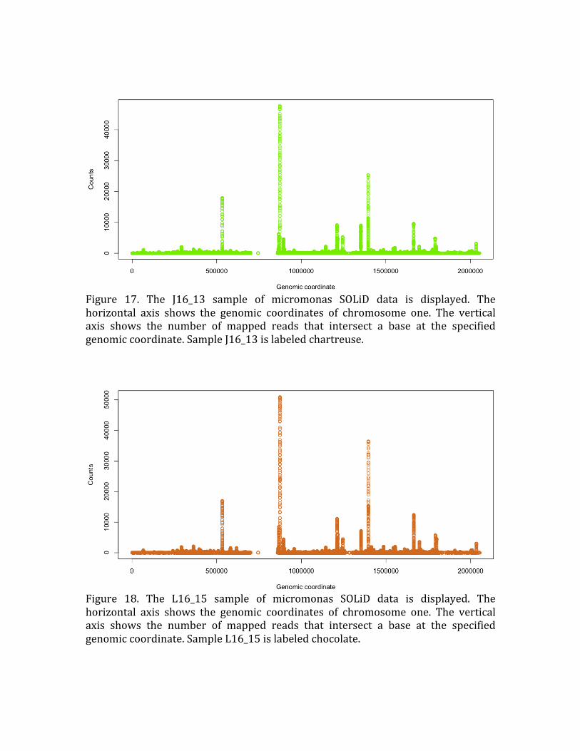
 Figure  17.  The  J16_13  sample  of  micromonas  SOLiD  data  is  displayed.  The 

horizontal  axis  shows  the  genomic  coordinates  of  chromosome  one.  The  vertical 

axis  shows  the  number  of  mapped  reads  that  intersect  a  base  at  the  specified 

genomic coordinate. Sample J16_13 is labeled chartreuse.  

 

 Figure  18.  The  L16_15  sample  of  micromonas  SOLiD  data  is  displayed.  The 

horizontal  axis  shows  the  genomic  coordinates  of  chromosome  one.  The  vertical axis  shows  the  number  of  mapped  reads  that  intersect  a  base  at  the  specified 

genomic coordinate. Sample L16_15 is labeled chocolate.  

  

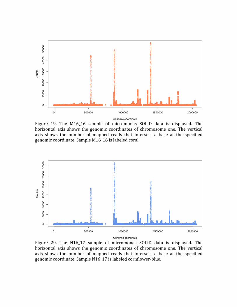
 Figure  19.  The  M16_16  sample  of  micromonas  SOLiD  data  is  displayed.  The 

horizontal  axis  shows  the  genomic  coordinates  of  chromosome  one.  The  vertical 

axis  shows  the  number  of  mapped  reads  that  intersect  a  base  at  the  specified 

genomic coordinate. Sample M16_16 is labeled coral. 

 

 Figure  20.  The  N16_17  sample  of  micromonas  SOLiD  data  is  displayed.  The 

horizontal  axis  shows  the  genomic  coordinates  of  chromosome  one.  The  vertical 

axis  shows  the  number  of  mapped  reads  that  intersect  a  base  at  the  specified genomic coordinate. Sample N16_17 is labeled cornflower‐blue. 

 

 

 Figure  21.  The  O16_18  sample  of  micromonas  SOLiD  data  is  displayed.  The 

horizontal  axis  shows  the  genomic  coordinates  of  chromosome  one.  The  vertical axis  shows  the  number  of  mapped  reads  that  intersect  a  base  at  the  specified 

genomic coordinate. Sample O16_18 is labeled cyan. 

 

 Figure  22.  The  Q16_20  sample  of  micromonas  SOLiD  data  is  displayed.  The 

horizontal  axis  shows  the  genomic  coordinates  of  chromosome  one.  The  vertical 

axis  shows  the  number  of  mapped  reads  that  intersect  a  base  at  the  specified 

genomic coordinate. Sample Q16_20 is labeled dark cyan.  

 

 Figure  23.  The  R16_21  sample  of  micromonas  SOLiD  data  is  displayed.  The 

horizontal  axis  shows  the  genomic  coordinates  of  chromosome  one.  The  vertical 

axis  shows  the  number  of  mapped  reads  that  intersect  a  base  at  the  specified genomic coordinate. Sample R16_21 is labeled dark goldenrod. 

 

 Figure  24.  The  S16_22  sample  of  micromonas  SOLiD  data  is  displayed.  The horizontal  axis  shows  the  genomic  coordinates  of  chromosome  one.  The  vertical 

axis  shows  the  number  of  mapped  reads  that  intersect  a  base  at  the  specified genomic coordinate. Sample S16_22 is labeled dark brown.  

 

 

 Figure  25.  The  U21_01  sample  of  micromonas  SOLiD  data  is  displayed.  The 

horizontal  axis  shows  the  genomic  coordinates  of  chromosome  one.  The  vertical 

axis  shows  the  number  of  mapped  reads  that  intersect  a  base  at  the  specified 

genomic coordinate. Sample U21_01 is labeled blue‐violet.  

 Figure  26.  The  V21_02  sample  of  micromonas  SOLiD  data  is  displayed.  The 

horizontal  axis  shows  the  genomic  coordinates  of  chromosome  one.  The  vertical axis  shows  the  number  of  mapped  reads  that  intersect  a  base  at  the  specified 

genomic coordinate. Sample V21_02 is labeled dark aquamarine.  

 

 Figure  27.  The  W21_03  sample  of  micromonas  SOLiD  data  is  displayed.  The 

horizontal  axis  shows  the  genomic  coordinates  of  chromosome  one.  The  vertical axis  shows  the  number  of  mapped  reads  that  intersect  a  base  at  the  specified 

genomic coordinate. Sample W21_03 is labeled dark chocolate. 

 

 Figure  28.  The  Z21_02  sample  of  micromonas  SOLiD  data  is  displayed.  The 

horizontal  axis  shows  the  genomic  coordinates  of  chromosome  one.  The  vertical 

axis  shows  the  number  of  mapped  reads  that  intersect  a  base  at  the  specified 

genomic coordinate. Sample Z21_02 is labeled dark antique white.   

 

 

References 

Li, H. et al.  (2009) Fast  and accurate  short  read alignment with Burrows‐Wheeler 

transform. Bioinformatics, 25, 1754‐1760.   

Langmead, B. et al.  (2009) Ultrafast and memory‐efficient alignment of  short DNA 

sequences to the human genome. Genome Biology, 10:R25, 1‐10.  

Homer,  N.  et  al.  (2009)  BFAST:  An  alignment  tool  for  large  scale  genome 

resequencing. PLoS ONE, 4(11), e7767: 1‐12.