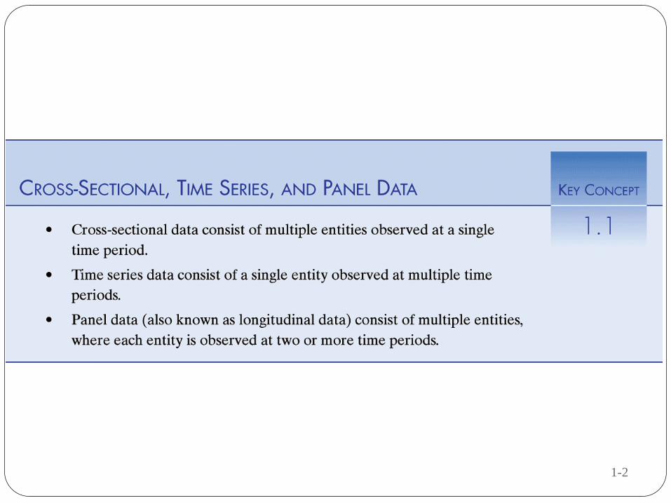
Types of economic data

Time series data

Cross-sectional data

Panel data

1

1-2

1-3

1-4

1-5

The distinction between qualitative and

quantitative data

The previous data sets can be used to illustrate an important

distinction between types of data. The microeconomist’s data on

sales will have a number corresponding to each firm surveyed (e.g.

last month’s sales in the first company surveyed were £20,000).

This is referred to as quantitative data.

The labor economist, when asking whether or not each surveyed

employee belongs to a union, receives either a Yes or a No answer.

These answers are referred to as qualitative data. Such data

arise often in economics when choices are involved (e.g.

the choice to buy or not buy a product, to take public transport or

a private car, to join or not to join a club).

6

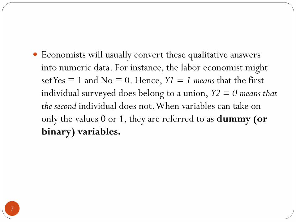
Economists will usually convert these qualitative answers

into numeric data. For instance, the labor economist might

set Yes = 1 and No = 0. Hence, Y1 = 1 means that the first

individual surveyed does belong to a union, Y2 = 0 means that

the second individual does not. When variables can take on

only the values 0 or 1, they are referred to as dummy (or

binary) variables.

7

What is

Descriptive Research?

Involves gathering data that describe events and then

organizes, tabulates, depicts, and describes the data.

Uses description as a tool to organize data into patterns that

emerge during analysis.

Often uses visual aids such as graphs and charts to aid the

reader

8

Descriptive Research

takes a “what is” approach

What is the best way to provide access to computer equipment

in schools?

Do teachers hold favorable attitudes toward using computers in

schools?

What have been the reactions of school administrators to

technological innovations in teaching?

9

Descriptive Research

We will want to see if a value or sample comes from a known

population. That is, if I were to give a new cancer treatment

to a group of patients, I would want to know if their survival

rate, for example, was different than the survival rate of

those who do not receive the new treatment. What we are

testing then is whether the sample patients who receive the

new treatment come from the population we already know

about (cancer patients without the treatment).

10

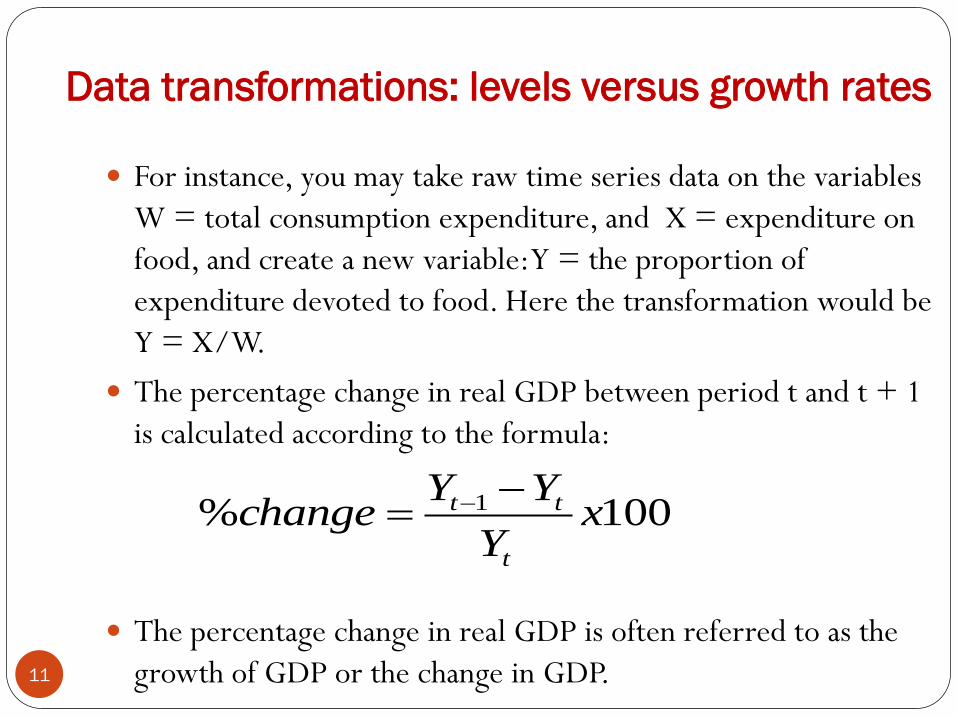
Data transformations: levels versus growth rates

For instance, you may take raw time series data on the variables

W = total consumption expenditure, and X = expenditure on

food, and create a new variable: Y = the proportion of

expenditure devoted to food. Here the transformation would be

Y = X/W.

The percentage change in real GDP between period t and t + 1

is calculated according to the formula:

The percentage change in real GDP is often referred to as the

growth of GDP or the change in GDP.

100% 1 xY

YYchange

t

tt

11

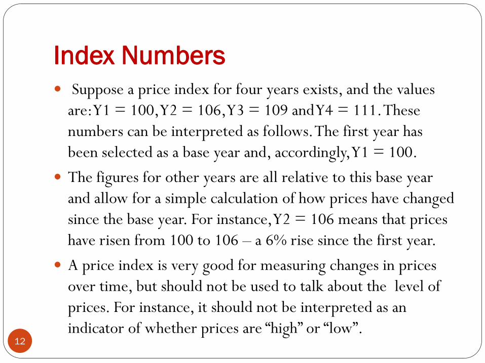
Index Numbers

Suppose a price index for four years exists, and the values

are: Y1 = 100, Y2 = 106, Y3 = 109 and Y4 = 111. These

numbers can be interpreted as follows. The first year has

been selected as a base year and, accordingly, Y1 = 100.

The figures for other years are all relative to this base year

and allow for a simple calculation of how prices have changed

since the base year. For instance, Y2 = 106 means that prices

have risen from 100 to 106 – a 6% rise since the first year.

A price index is very good for measuring changes in prices

over time, but should not be used to talk about the level of

prices. For instance, it should not be interpreted as an

indicator of whether prices are “high” or “low”. 12

Obtaining Data

Most macroeconomic data is collected through a system of

national accounts

Microeconomic data is usually collected by surveys of

households, employment and businesses, which are often

available from the same sources.

Two of the more popular ones are Datastream by Thomson

Financial (http://www.datastream.com/) and Wharton

Research Data Services (http://wrds.wharton.upenn.edu/).

With regards to free data, a more limited choice of financial

data is available through popular Internet ports such as Yahoo!

(http://finance.yahoo.com).

13

Working with data: graphical

methods

it is important for you to summarize

Charts and tables are very useful ways of presenting your

data. There are many different types (e.g. bar chart, pie chart,

etc.).

With time series data, a chart that shows how a variable

evolves over time is often very informative. However, in the

case of cross-sectional data, such methods are not

appropriate and we must summarize the data in other ways

14

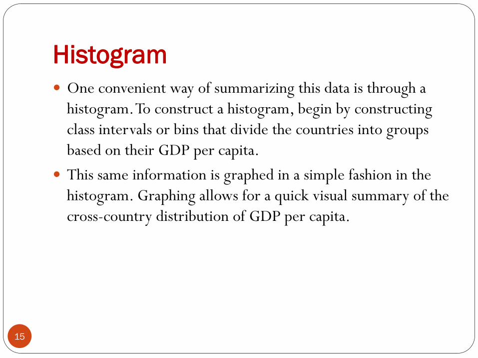
Histogram

One convenient way of summarizing this data is through a

histogram. To construct a histogram, begin by constructing

class intervals or bins that divide the countries into groups

based on their GDP per capita.

This same information is graphed in a simple fashion in the

histogram. Graphing allows for a quick visual summary of the

cross-country distribution of GDP per capita.

15

XY Plots the relationships between two or more variables. For instance:

“Are higher education levels and work experience associated

with higher wages among workers in a given industry?” “Are

changes in the money supply a reliable indicator of inflation

changes?” “Do differences in capital investment explain why

some countries are growing faster than others?”

graphical methods can be used to draw out some simple aspects

of the relationship between two variables. XY-plots (also called

scatter diagrams) are particularly useful.

The XY-plot can be used to give a quick visual impression of the

relationship between deforestation and population density.

16

Mean

The mean is the statistical term for the average. The mathematical

formula for the mean is given by:

N: sample size

∑: summation operator

N

Y

Y

N

i

i 1

17

Standard Deviation

A more common measure of dispersion is the standard

deviation. (Confusingly atisticians refer to the square of the

standard deviation as the variance.) Its mathmatical formula

is given by:

1

)(1

2

N

YYN

i

i

18

Correlation

Correlation is an important way of numerically quantifying

the relationship between two variables:

rxy the correlation between variables X and Y,

N

i

i

N

i

i

N

i

ii

xy

XXYY

XXYY

r

1

2

1

2

1

)()(

))((

19

Properties of correlation 1. r always lies between -1 and 1, which may be written as -1<r <1.

2. Positive values of r indicate a positive correlation between X and Y.

Negative values indicate a negative correlation. r = 0 indicates that X

and Y are uncorrelated.

3. Larger positive values of r indicate stronger positive correlation. r =

1 indicates perfect positive correlation. Larger negative values 1 of r

indicate stronger negative correlation. r =-1 indicates perfect negative

correlation.

4. The correlation between Y and X is the same as the correlation

between X and Y.

5. The correlation between any variable and itself (e.g. the correlation

between Y and Y) is 1

20

One of the most important things in empirical work is

knowing how to interpret your results. The house example

illustrates this difficulty well. It is not enough just to report a

number for a correlation (e.g. rXY = 0.54). Interpretation is

important too.

Interpretation requires a good intuitive knowledge of what a

correlation is in addition to a lot of common sense about the

economic phenomenon under study.

21

Correlation between several variables

For instance, house prices depend on the lot size, number of

bedrooms, number of bathrooms and many other

characteristics of the house.

if we have three variables, X, Y and Z, then there are three

possible correlations (i.e. rXY, rXZ and rYZ). However, if we

add a fourth variable, W, the number increases to six (i.e. rXY,

rXZ, rXW, rYZ, rYW and rZW). In general, for M different

variables there will be M x (M - 1)/2 possible correlations. A

convenient way of ordering all these correlations is to

construct a matrix or table.

22

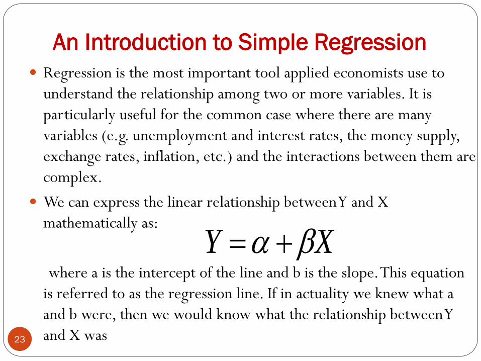
An Introduction to Simple Regression

Regression is the most important tool applied economists use to

understand the relationship among two or more variables. It is

particularly useful for the common case where there are many

variables (e.g. unemployment and interest rates, the money supply,

exchange rates, inflation, etc.) and the interactions between them are

complex.

We can express the linear relationship between Y and X

mathematically as:

where a is the intercept of the line and b is the slope. This equation

is referred to as the regression line. If in actuality we knew what a

and b were, then we would know what the relationship between Y

and X was

XY

23

4-24

4-25

4-26

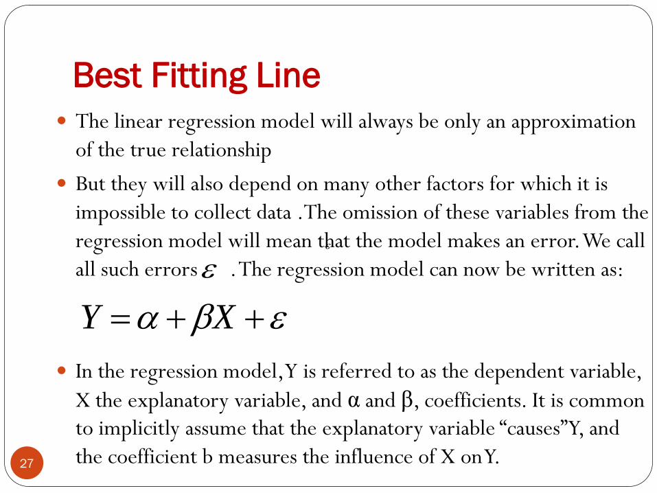
Best Fitting Line

The linear regression model will always be only an approximation

of the true relationship

But they will also depend on many other factors for which it is

impossible to collect data .The omission of these variables from the

regression model will mean that the model makes an error. We call

all such errors . The regression model can now be written as:

In the regression model, Y is referred to as the dependent variable,

X the explanatory variable, and α and β, coefficients. It is common

to implicitly assume that the explanatory variable “causes” Y, and

the coefficient b measures the influence of X on Y.

XY

27

OLS Estimation

The OLS estimator is the most popular estimator of β,

OLS estimator is chosen to minimize:

OLS estimator

2

2

)ˆvar(iX

N

i

iSSE1

2

N

i

i

N

i

ii

X

YX

1

2

1

28

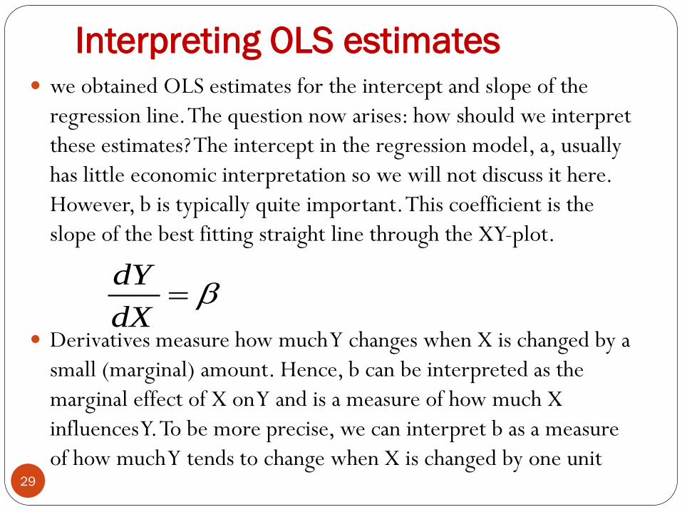
Interpreting OLS estimates we obtained OLS estimates for the intercept and slope of the

regression line. The question now arises: how should we interpret

these estimates? The intercept in the regression model, a, usually

has little economic interpretation so we will not discuss it here.

However, b is typically quite important. This coefficient is the

slope of the best fitting straight line through the XY-plot.

Derivatives measure how much Y changes when X is changed by a

small (marginal) amount. Hence, b can be interpreted as the

marginal effect of X on Y and is a measure of how much X

influences Y. To be more precise, we can interpret b as a measure

of how much Y tends to change when X is changed by one unit

dX

dY

29

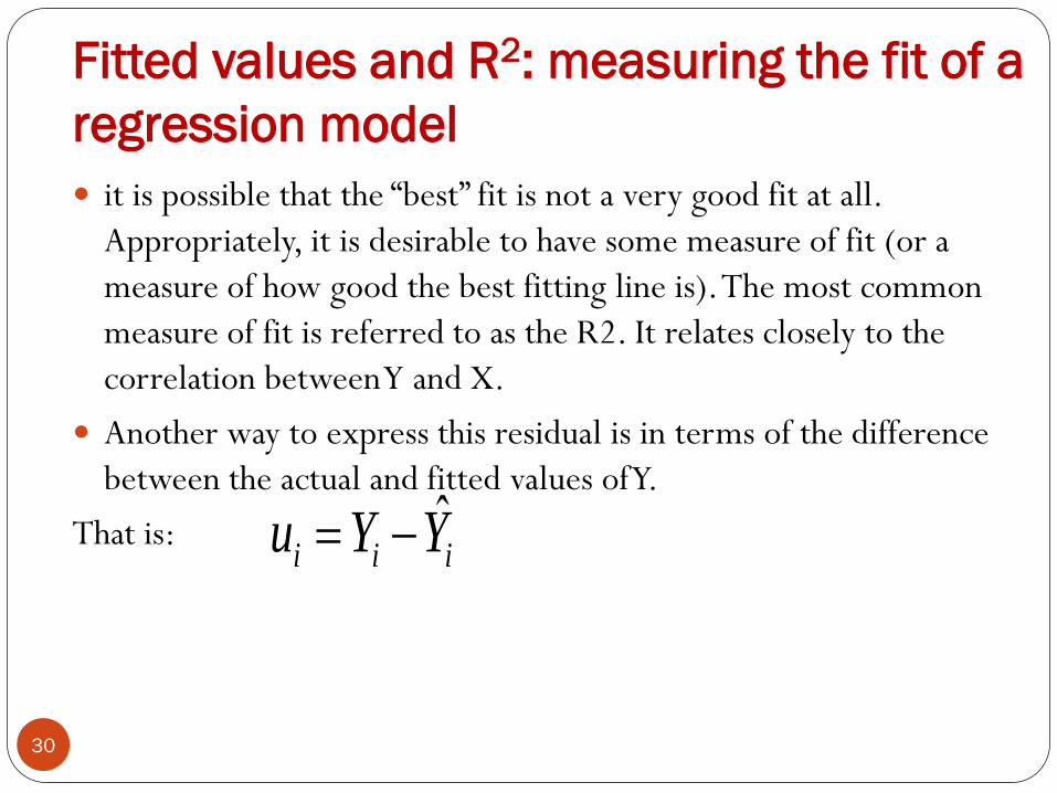
Fitted values and R2: measuring the fit of a

regression model

it is possible that the “best” fit is not a very good fit at all.

Appropriately, it is desirable to have some measure of fit (or a

measure of how good the best fitting line is). The most common

measure of fit is referred to as the R2. It relates closely to the

correlation between Y and X.

Another way to express this residual is in terms of the difference

between the actual and fitted values of Y.

That is: iii YYu ˆ

30

Recall that variance is the measure of dispersion or variability of

the data. Here we define a closely related concept, the total sum

of squares or TSS:

The regression model seeks to explain the variability in Y

through the explanatory variable X. It can be shown that the

total variability in Y can be broken into two parts as:

TSS=RSS + SSR

where RSS is the regression sum of squares, a measure of the

explanation provided by the regression model.

RSS is given by:

2

1

)( YYTSSN

i

i

2

1

)ˆ( YYRSSN

i

i

31

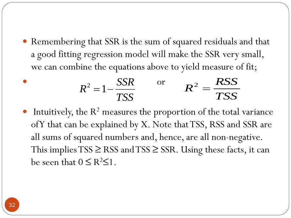
Remembering that SSR is the sum of squared residuals and that

a good fitting regression model will make the SSR very small,

we can combine the equations above to yield measure of fit;

or

Intuitively, the R2 measures the proportion of the total variance

of Y that can be explained by X. Note that TSS, RSS and SSR are

all sums of squared numbers and, hence, are all non-negative.

This implies TSS ≥ RSS and TSS ≥ SSR. Using these facts, it can

be seen that 0 ≤ R2≤1.

TSS

SSRR 12

TSS

RSSR 2

32

Further intuition about this measure of fit can be obtained by

noting that small values of SSR indicate that the regression

model is fitting well. A regression line which fits all the data

points perfectly in the XY-plot will have no errors and hence

SSR = 0 and R2 = 1. Looking at the formula above, you can

see that values of R2 near 1 imply a good fit and that R2 = 1

implies a perfect fit. In sum, high values of R2 imply a good fit

and low values a bad fit.

33

7-34

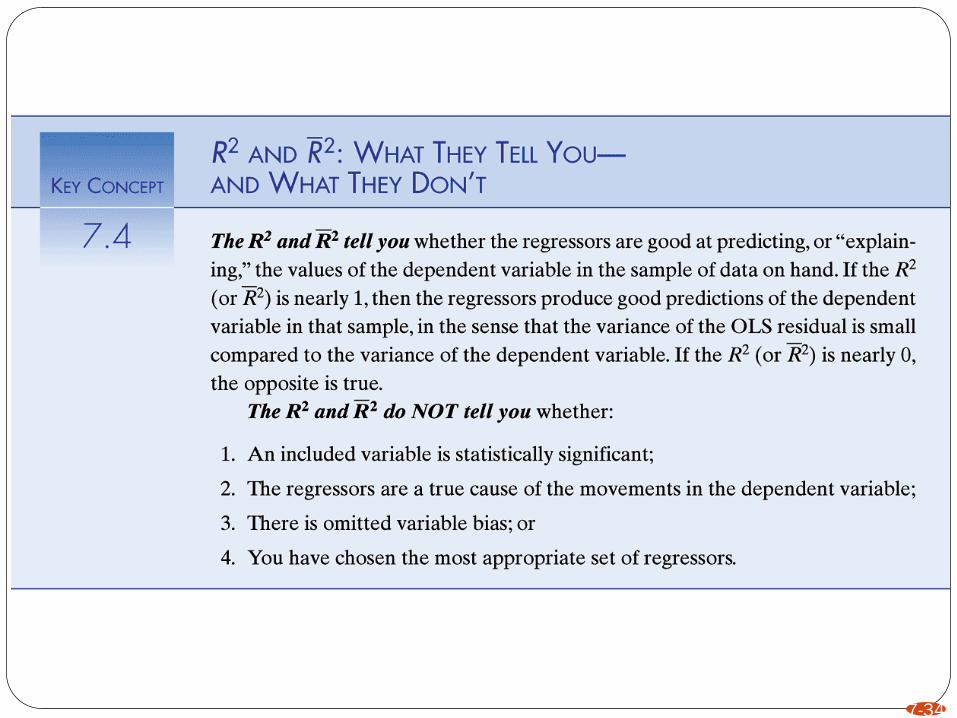
Hypothesis Testing

The other major activity of the empirical researcher is

hypothesis testing. An example of a hypothesis that a

researcher may want to test is β = 0. If the latter hypothesis is

true, then this means that the explanatory variable has no

explanatory power. Hypothesis testing procedures allow us to

carry out such tests

35

Hypothesis Testing

Purpose: make inferences about a population parameter by

analyzing differences between observed sample statistics and the

results one expects to obtain if some underlying assumption is

true.

• Null hypothesis:

• Alternative hypothesis:

If the null hypothesis is rejected then the alternative hypothesis

is accepted.

n

XZ

KbytesH

KbytesH

5.12:

5.12:

1

0

36

Hypothesis Testing

A sample of 50 files from a file system is selected. The sample

mean is 12.3Kbytes. The standard deviation is known to be

0.5 Kbytes.

Confidence: 0.95

KbytesH

KbytesH

5.12:

5.12:

1

0

Critical value =NORMINV(0.05,0,1)= -1.645.

Region of non-rejection: Z ≥ -1.645.

So, do not reject Ho. (Z exceeds critical value)

37

Steps in Hypothesis Testing

1. State the null and alternative hypothesis.

2. Choose the level of significance a.

3. Choose the sample size n. Larger samples allow us to detect

even small differences between sample statistics and true

population parameters. For a given a, increasing n decreases b.

4. Choose the appropriate statistical technique and test statistic

to use (Z or t).

38

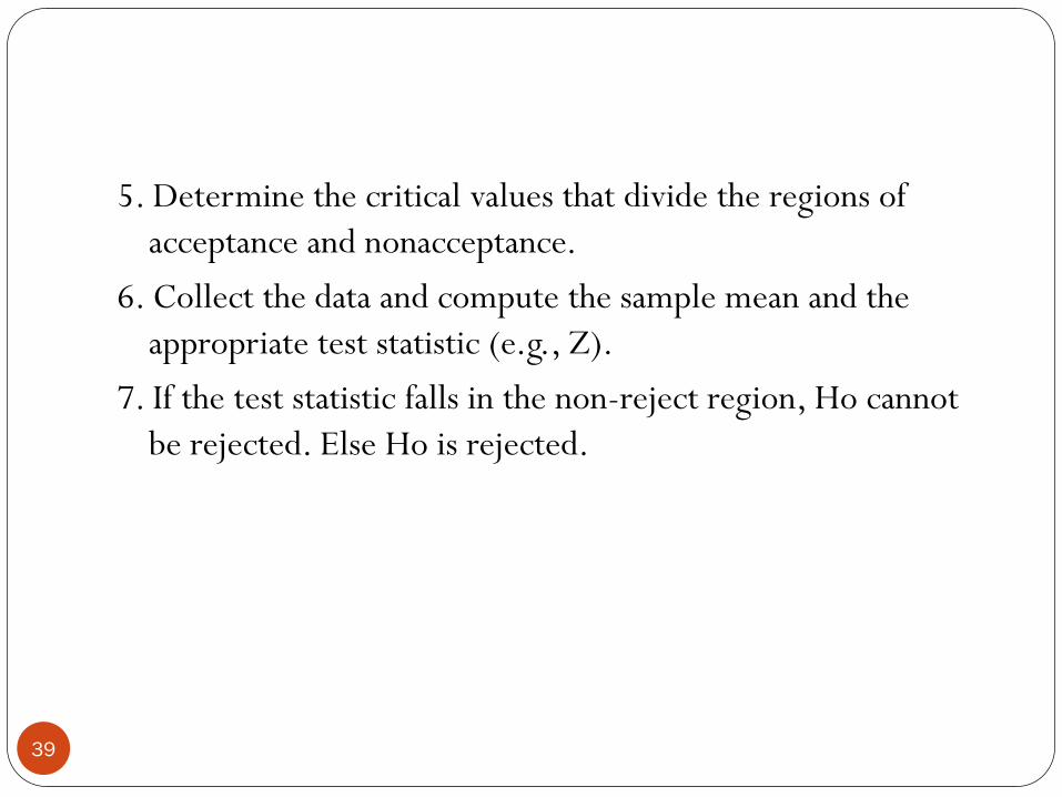
5. Determine the critical values that divide the regions of

acceptance and nonacceptance.

6. Collect the data and compute the sample mean and the

appropriate test statistic (e.g., Z).

7. If the test statistic falls in the non-reject region, Ho cannot

be rejected. Else Ho is rejected.

39

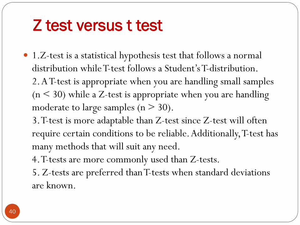
Z test versus t test

1.Z-test is a statistical hypothesis test that follows a normal

distribution while T-test follows a Student’s T-distribution.

2. A T-test is appropriate when you are handling small samples

(n < 30) while a Z-test is appropriate when you are handling

moderate to large samples (n > 30).

3. T-test is more adaptable than Z-test since Z-test will often

require certain conditions to be reliable. Additionally, T-test has

many methods that will suit any need.

4. T-tests are more commonly used than Z-tests.

5. Z-tests are preferred than T-tests when standard deviations

are known.

40

One tail versus two tail

we were only looking at one “tail” of the distribution at a time (either

on the positive side above the mean or the negative side below the

mean). With two-tail tests we will look for unlikely events on both

sides of the mean (above and below) at the same time.

So, we have learned four critical values.

1-tail 2-tail

α = .05 1.64 1.96, -1.96

α = .01 2.33 2.58/-2.58

Notice that you have two critical values for a 2-tail test, both positive

and negative. You will have only one critical value for a one-tail test

(which could be negative).

41

Which factors affect the accuracy of

the estimate 1. Having more data points improves accuracy of

estimation.

2. Having smaller errors improves accuracy of

estimation. Equivalently, if the SSR is small or the

variance of the errors is small, the accuracy of the estimation

will be improved.

3. Having a larger spread of values (i.e. a larger variance) of

the explanatory variable (X) improves accuracy of estimation.

42

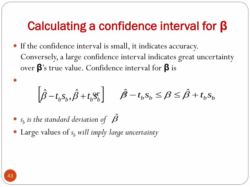
Calculating a confidence interval for β

If the confidence interval is small, it indicates accuracy.

Conversely, a large confidence interval indicates great uncertainty

over β’s true value. Confidence interval for β is

or

sb is the standard deviation of

Large values of sb will imply large uncertainty

bbbb stst ˆ,ˆ bbbb stst ˆˆ

43

Standard Deviation

Standard deviation of :

which measures the variability or uncertainty in ,

1. sb and, hence, the width of the confidence interval, varies

directly with SSR (i.e. more variable errors/residuals imply

less accurate estimation).

2. sb and, hence, the width of the confidence interval, vary

inversely with N (i.e. more data points imply more accurate

estimation).

3. sb and, hence, the width of the confidence interval, vary

inversely with Σ(Xi - X)2 (i.e. more variability in X implies more

accurate estimation).

2)()2( XXN

SSRs

i

b

44

The third number in the formula for the confidence interval is

tb. tb is a value taken from statistical tables for the Student-t

distribution.

1. tb decreases with N (i.e. the more data points you have

the smaller the confidence interval will be).

2. tb increases with the level of confidence you choose.

45

Testing whether β = 0

we say that this is a test of H0: β = 0 against H1: β ≠ 0

Note that, if b = 0 then X does not appear in the regression model; that

is, the explanatory variable fails to provide any explanatory power

whatsoever for the dependent variable.

hypothesis tests come with various levels of significance. If

you use the confidence interval approach to hypothesis testing,

then the level of significance is 100% minus the confidence level.

That is, if a 95% confidence interval does not include zero, then

you may say “I reject the hypothesis that β= 0 at the 5% level of

significance” (i.e. 100% - 95% = 5%). If you had used a 90%

confidence interval (and found it did not contain zero) then you

would say: “I reject the hypothesis that β = 0 at the 10% level of

significance.” 46

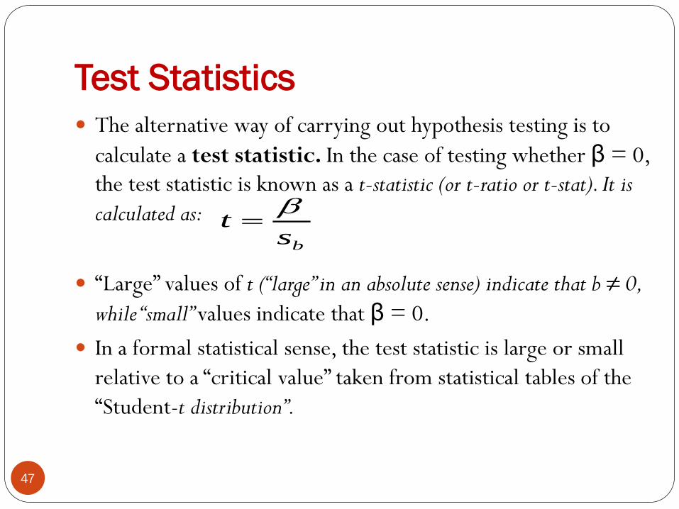
Test Statistics

The alternative way of carrying out hypothesis testing is to

calculate a test statistic. In the case of testing whether β = 0,

the test statistic is known as a t-statistic (or t-ratio or t-stat). It is

calculated as:

“Large” values of t (“large” in an absolute sense) indicate that b ≠ 0,

while “small” values indicate that β = 0.

In a formal statistical sense, the test statistic is large or small

relative to a “critical value” taken from statistical tables of the

“Student-t distribution”.

bst

47

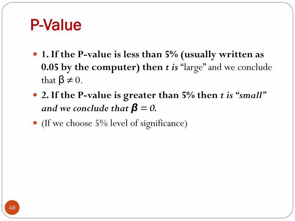
P-Value

1. If the P-value is less than 5% (usually written as

0.05 by the computer) then t is “large” and we conclude

that β ≠ 0.

2. If the P-value is greater than 5% then t is “small”

and we conclude that β = 0.

(If we choose 5% level of significance)

48

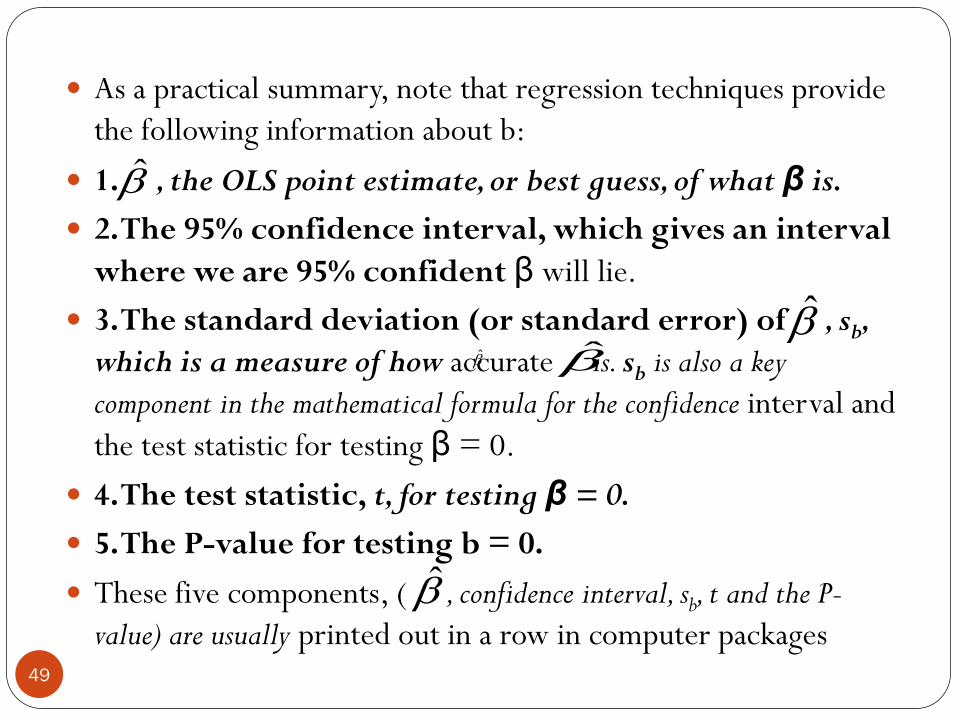
As a practical summary, note that regression techniques provide

the following information about b:

1. , the OLS point estimate, or best guess, of what β is.

2. The 95% confidence interval, which gives an interval

where we are 95% confident β will lie.

3. The standard deviation (or standard error) of , sb,

which is a measure of how accurate is. sb is also a key

component in the mathematical formula for the confidence interval and

the test statistic for testing β = 0.

4. The test statistic, t, for testing β = 0.

5. The P-value for testing b = 0.

These five components, ( , confidence interval, sb, t and the P-

value) are usually printed out in a row in computer packages

49

how regression results are presented and

interpreted?

Table 5.2 The regression of deforestation on population density.

Coefficient St.Er. t-stat. P-value Lower 95% Upper 95%

Intercept 0.599 0.112 5.341 1.15E – 06 0.375 0.824

X variable 0.0008 0.00011 7.227 5.5E – 10 0.00061 0.00107

= 0.000842, indicating that increasing population density by one person

per hectare is associated with an increase in deforestation rates of 0.000842%.

The columns labeled “Lower 95%” and “Upper 95%” give the lower and upper

bounds of the 95% confidence interval. For this data set, and as discussed

previously, the 95% confidence interval for β is [0.00061, 0.001075]. Thus, we

are 95% confident that the marginal effect of population density on

deforestation is between 0.00061% and 0.001075%.

50

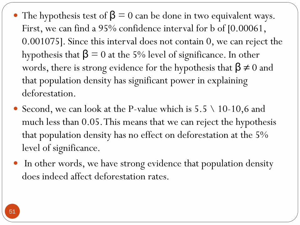
The hypothesis test of β = 0 can be done in two equivalent ways.

First, we can find a 95% confidence interval for b of [0.00061,

0.001075]. Since this interval does not contain 0, we can reject the

hypothesis that β = 0 at the 5% level of significance. In other

words, there is strong evidence for the hypothesis that β ≠ 0 and

that population density has significant power in explaining

deforestation.

Second, we can look at the P-value which is 5.5 \ 10-10,6 and

much less than 0.05. This means that we can reject the hypothesis

that population density has no effect on deforestation at the 5%

level of significance.

In other words, we have strong evidence that population density

does indeed affect deforestation rates.

51

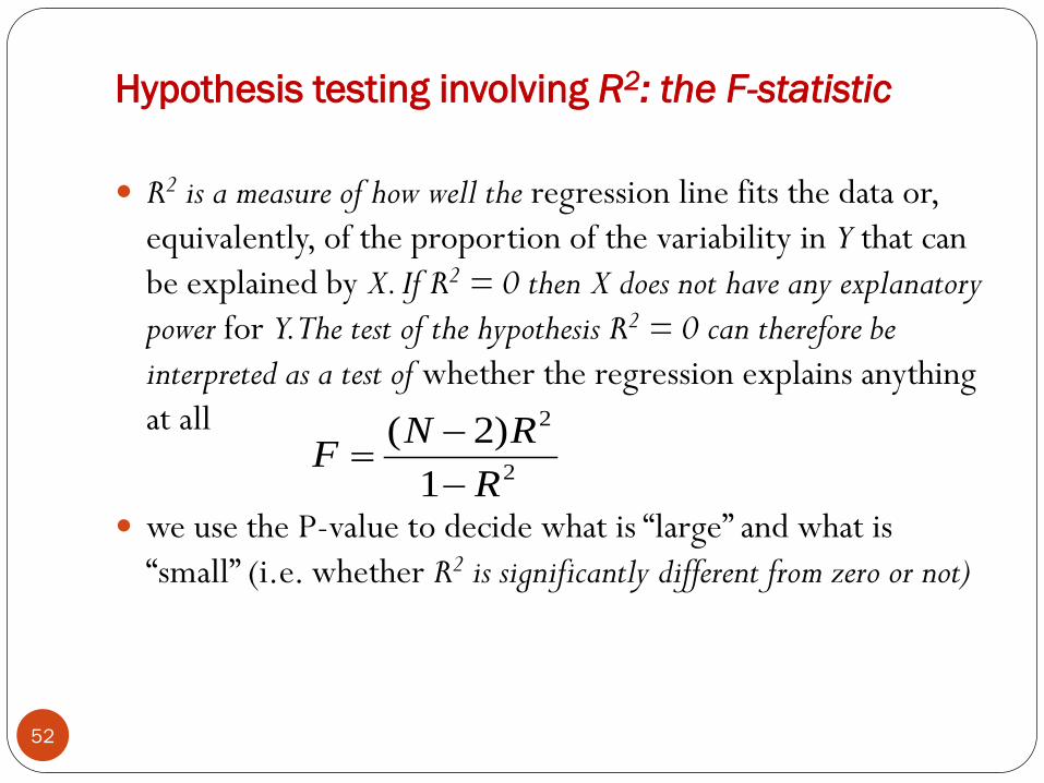
Hypothesis testing involving R2: the F-statistic

R2 is a measure of how well the regression line fits the data or,

equivalently, of the proportion of the variability in Y that can

be explained by X. If R2 = 0 then X does not have any explanatory

power for Y. The test of the hypothesis R2 = 0 can therefore be

interpreted as a test of whether the regression explains anything

at all

we use the P-value to decide what is “large” and what is

“small” (i.e. whether R2 is significantly different from zero or not)

2

2

1

)2(

R

RNF

52

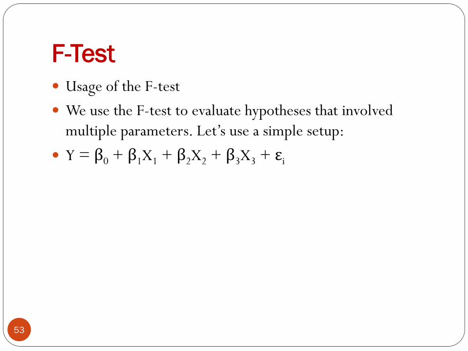
F-Test

Usage of the F-test

We use the F-test to evaluate hypotheses that involved

multiple parameters. Let’s use a simple setup:

Y = β0 + β1X1 + β2X2 + β3X3 + εi

53

F-Test

For example, if we wanted to know how economic policy

affects economic growth, we may include several policy

instruments (balanced budgets, inflation, trade-openness, &c)

and see if all of those policies are jointly significant. After all,

our theories rarely tell

us which variable is important, but rather a broad category of

variables.

54

F-statistic

The test is performed according to the following strategy:

1. If Significance F is less than 5% (i.e. 0.05), we

conclude R2 ≠ 0.

2. If Significance F is greater than 5% (i.e. 0.05), we

conclude R2 = 0.

55

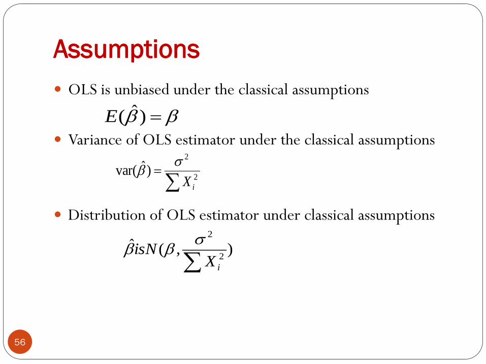
Assumptions

OLS is unbiased under the classical assumptions

Variance of OLS estimator under the classical assumptions

Distribution of OLS estimator under classical assumptions

)ˆ(E

2

2

)ˆvar(iX

),(ˆ2

2

iXisN

56

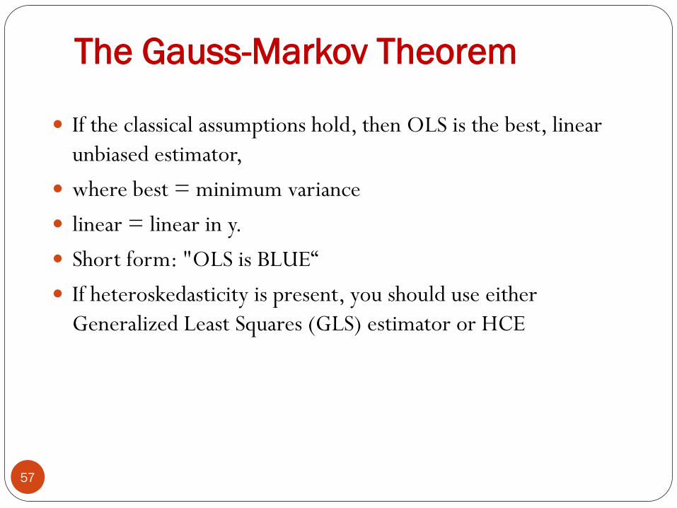
The Gauss-Markov Theorem

If the classical assumptions hold, then OLS is the best, linear

unbiased estimator,

where best = minimum variance

linear = linear in y.

Short form: "OLS is BLUE“

If heteroskedasticity is present, you should use either

Generalized Least Squares (GLS) estimator or HCE

57

Heteroscedasticity Heteroskedasticity occurs when the error variance differs across

observations. :

Errors mis-pricing of houses

If a house sells for much more (or less) than comparable houses, then

it will have a big error

Suppose small houses all very similar, then unlikely to be large pricing

errors

Suppose big houses can be very different than one another, then

possible to have large pricing errors

If this story is true, then expect errors for big houses to have larger

variance than for small houses Statistically: heteroskedasticity is

present and is associated with the size of the house

58

Assumption 2 replaced by for i = 1, ..,N.

Note: wi varies with i so error variance differs across observations

GLS proceeds by transforming model and then using OLS on

transformed model

Transformation comes down to dividing all observations by wi

Problem with GLS: in practice, it can be hard to figure out what wi is

To do GLS need to find answer to questions like:

Is wi proportional to an explanatory variable? If yes, then which one?

Thus HCEs are popular. (Gretl)

Use OLS estimates, but corrects its variance so as to get

correct confidence intervals, hypothesis tests, etc.

Advantages: HCEs are easy to calculate and you do not need to know

the form that the heteroskedasticity takes.

Disadvantages: HCEs are not as e¢ cient as the GLS estimator

(i.e.they will have larger variance).

))ˆ(var(

22)var( ii

))ˆ(var(

59

If heteroskedasticity is NOT present, then OLS is .ne (it is BLUE).

But if it is present, you should use GLS or a HCE

Thus, it is important to know if heteroskedasticity is present.

There are many tests, such as;

White test and the Breusch Pagan test

These are done in Gretl

60

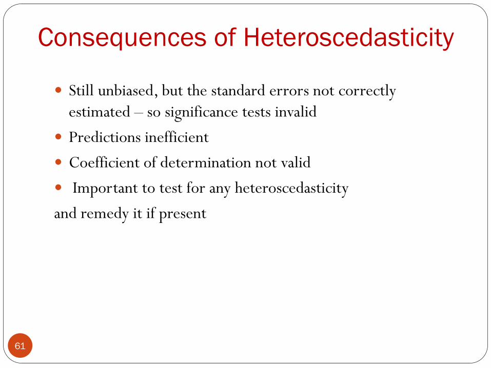
Still unbiased, but the standard errors not correctly

estimated – so significance tests invalid

Predictions inefficient

Coefficient of determination not valid

Important to test for any heteroscedasticity

and remedy it if present

Consequences of Heteroscedasticity

61

Detecting Heteroscedasticity (II)

Number of formal tests:

Koenkar test – linear form of heteroscedasticity assumption

Regress the square of the estimated error term on the explanatory

variables, if these variables are jointly significant, then you reject the

null of homoscedastic errors

White test – most popular, available in Eviews

Same like Koenkar test, but you include also the squares of

explanatory variables and their cross products (do not include cross-

products, if you have many explanatory variables – multicollinearity

likely)

62

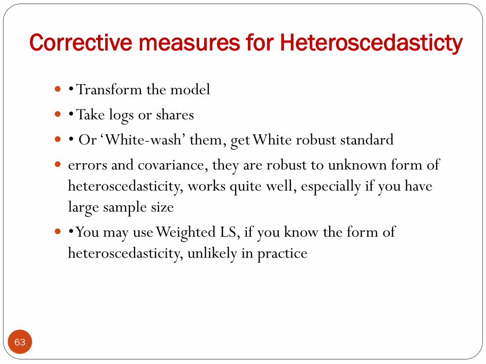
Corrective measures for Heteroscedasticty

• Transform the model

• Take logs or shares

• Or ‘White-wash’ them, get White robust standard

errors and covariance, they are robust to unknown form of

heteroscedasticity, works quite well, especially if you have

large sample size

• You may use Weighted LS, if you know the form of

heteroscedasticity, unlikely in practice

63

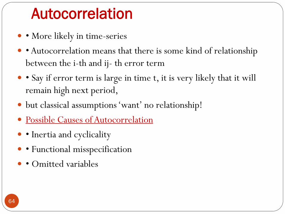
Autocorrelation

• More likely in time-series

• Autocorrelation means that there is some kind of relationship

between the i-th and ij- th error term

• Say if error term is large in time t, it is very likely that it will

remain high next period,

but classical assumptions ‘want’ no relationship!

Possible Causes of Autocorrelation

• Inertia and cyclicality

• Functional misspecification

• Omitted variables

64

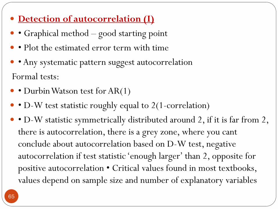
Detection of autocorrelation (I)

• Graphical method – good starting point

• Plot the estimated error term with time

• Any systematic pattern suggest autocorrelation

Formal tests:

• Durbin Watson test for AR(1)

• D-W test statistic roughly equal to 2(1-correlation)

• D-W statistic symmetrically distributed around 2, if it is far from 2,

there is autocorrelation, there is a grey zone, where you cant

conclude about autocorrelation based on D-W test, negative

autocorrelation if test statistic ‘enough larger’ than 2, opposite for

positive autocorrelation • Critical values found in most textbooks,

values depend on sample size and number of explanatory variables

65

Corrective Measures of Autocorrelation

• First differencing

• Quasi differencing

• Or ‘Newey-West wash’, analogy of Whitewashing, it makes

your standard errors and covariance robust to unknown form

of autocorrelation, available for E-views

66

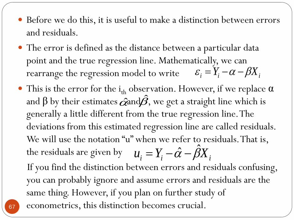
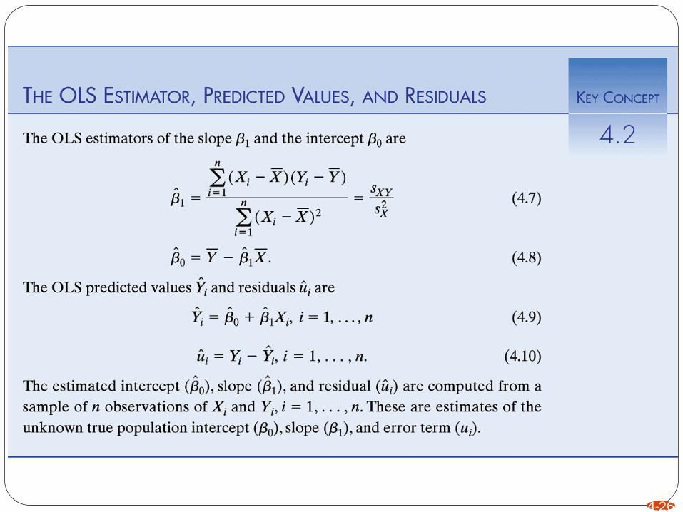
Before we do this, it is useful to make a distinction between errors

and residuals.

The error is defined as the distance between a particular data

point and the true regression line. Mathematically, we can

rearrange the regression model to write

This is the error for the ith observation. However, if we replace α

and β by their estimates and , we get a straight line which is

generally a little different from the true regression line. The

deviations from this estimated regression line are called residuals.

We will use the notation “u” when we refer to residuals. That is,

the residuals are given by

If you find the distinction between errors and residuals confusing,

you can probably ignore and assume errors and residuals are the

same thing. However, if you plan on further study of

econometrics, this distinction becomes crucial.

iii XY

iii XYu ˆˆ

67

The residuals are the vertical difference between a data point

and the line. A good fitting line will have small residuals.

The usual way of measuring the size of the residuals is by

means of the sum of squared residuals (SSR), which is given

by:

We want to find the best fitting line which minimizes the

sum of squared residuals. For this reason, estimates found in

this way are called least squares estimates

N

i

iuSSR1

2

68

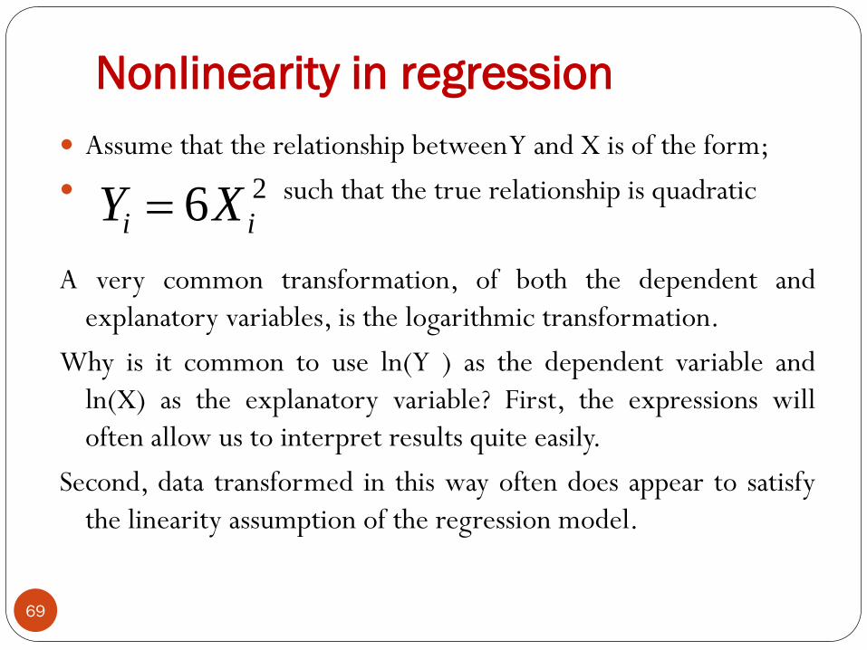
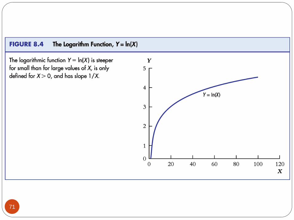
Nonlinearity in regression

Assume that the relationship between Y and X is of the form;

such that the true relationship is quadratic

A very common transformation, of both the dependent and

explanatory variables, is the logarithmic transformation.

Why is it common to use ln(Y ) as the dependent variable and

ln(X) as the explanatory variable? First, the expressions will

often allow us to interpret results quite easily.

Second, data transformed in this way often does appear to satisfy

the linearity assumption of the regression model.

26 ii XY

69

Nonlinearity in regression

β can be interpreted as an elasticity. Recall that, in the basic

regression without logs, we said that “Y tends to change by b

units for a one unit change in X ”. In the regression

containing both logged dependent and explanatory variables,

we can now say that “Y tends to change by β percent for a

one percent change in X ”. That is, instead of having to worry

about units of measurements, regression results using logged

variables are always interpreted as elasticities.

)(ln)ln( XY

70

71

8-72

8-73