
Tutoriel
384
-
Upload
davidusc2008 -
Category
Documents
-
view
202 -
download
8
Transcript of Tutoriel


Part Number: Aspen Plus® 11.1September 2001Copyright (c) 1981-2001 by Aspen Technology, Inc. All rights reserved.
Aspen Plus®, Aspen Properties®, Aspen Engineering Suite, AspenTech®, ModelManager, the aspen leaf logo andPlantelligence are trademarks or registered trademarks of Aspen Technology, Inc., Cambridge, MA.
BATCHFRAC and RATEFRAC are trademarks of Koch Engineering Company, Inc.
All other brand and product names are trademarks or registered trademarks of their respective companies.
This manual is intended as a guide to using AspenTech's software. This documentation contains AspenTechproprietary and confidential information and may not be disclosed, used, or copied without the prior consent ofAspenTech or as set forth in the applicable license agreement. Users are solely responsible for the proper use of thesoftware and the application of the results obtained.
Although AspenTech has tested the software and reviewed the documentation, the sole warranty for the softwaremay be found in the applicable license agreement between AspenTech and the user. ASPENTECH MAKES NOWARRANTY OR REPRESENTATION, EITHER EXPRESSED OR IMPLIED, WITH RESPECT TO THISDOCUMENTATION, ITS QUALITY, PERFORMANCE, MERCHANTABILITY, OR FITNESS FOR APARTICULAR PURPOSE.
CorporateAspen Technology, Inc.Ten Canal ParkCambridge, MA 02141-2201USAPhone: (1) (617) 949-1021Toll Free: (1) (888) 996-7001Fax: (1) (617) 949-1724URL: http://www.aspentech.com
DivisionDesign, Simulation and Optimization SystemsAspen Technology, Inc.Ten Canal ParkCambridge, MA 02141-2201USAPhone: (617) 949-1000Fax: (617) 949-1030

Aspen Plus 11.1 Unit Operation Models Contents •••• iii
Contents
For More Information......................................................................................................... xiTechnical Support ............................................................................................................xiii
Contacting Customer Support ..............................................................................xiiiHours ....................................................................................................................xiiiPhone.................................................................................................................... xivFax......................................................................................................................... xvE-mail .................................................................................................................... xv
Mixers and Splitters 1-1Mixer Reference...............................................................................................................1-2
Flowsheet Connectivity for Mixer .......................................................................1-2Specifying Mixer..................................................................................................1-3EO Usage Notes for Mixer...................................................................................1-4
FSplit Reference...............................................................................................................1-5Flowsheet Connectivity for FSplit .......................................................................1-5Specifying FSplit..................................................................................................1-6EO Usage Notes for FSplit...................................................................................1-7
SSplit Reference...............................................................................................................1-8Flowsheet Connectivity for SSplit .......................................................................1-8Specifying SSplit..................................................................................................1-8
Separators 2-1Flash2 Reference ..............................................................................................................2-2
Flowsheet Connectivity for Flash2 ......................................................................2-2Specifying Flash2.................................................................................................2-3EO Usage Notes for Flash2..................................................................................2-3
Flash3 Reference ..............................................................................................................2-4Flowsheet Connectivity for Flash3 ......................................................................2-4Specifying Flash3.................................................................................................2-5
Decanter Reference ..........................................................................................................2-6Flowsheet Connectivity for Decanter...................................................................2-6Specifying Decanter .............................................................................................2-7EO Usage Notes for Decanter ..............................................................................2-9
Sep Reference.................................................................................................................2-10Flowsheet Connectivity for Sep .........................................................................2-10
iv •••• Contents Aspen Plus 11.1 Unit Operation Models
Specifying Sep....................................................................................................2-10EO Usage Notes for Sep.....................................................................................2-11
Sep2 Reference...............................................................................................................2-12Flowsheet Connectivity for Sep2 .......................................................................2-12Specifying Sep2..................................................................................................2-12EO Usage Notes for Sep2...................................................................................2-13
Heat Exchangers 3-1Heater Reference ..............................................................................................................3-2
Flowsheet Connectivity for Heater ......................................................................3-2Specifying Heater.................................................................................................3-3EO Usage Notes for Heater..................................................................................3-3
HeatX Reference ..............................................................................................................3-4Flowsheet Connectivity for HeatX.......................................................................3-5Specifying HeatX .................................................................................................3-6EO Usage Notes for HeatX ................................................................................3-18
MHeatX Reference.........................................................................................................3-19Flowsheet Connectivity for MHeatX .................................................................3-19Specifying MHeatX............................................................................................3-20
Hetran Reference............................................................................................................3-23Flowsheet Connectivity for Hetran ....................................................................3-23Specifying Hetran...............................................................................................3-24
Aerotran Reference ........................................................................................................3-25Flowsheet Connectivity for Aerotran.................................................................3-25Specifying Aerotran ...........................................................................................3-26
HxFlux Reference ..........................................................................................................3-27Flowsheet Connectivity for HxFlux...................................................................3-27Specifying HxFlux .............................................................................................3-27Convective Heat Transfer...................................................................................3-28Log-Mean Temperature Difference ...................................................................3-28EO Usage Notes for HXFlux .............................................................................3-28
HTRI-Xist Reference .....................................................................................................3-29Flowsheet Connectivity for HTRI-Xist..............................................................3-29Specifying HTRI-Xist ........................................................................................3-30
Columns 4-1DSTWU Reference ..........................................................................................................4-3
Flowsheet Connectivity for DSTWU...................................................................4-4Specifying DSTWU .............................................................................................4-4
Distl Reference.................................................................................................................4-5Flowsheet Connectivity for Distl .........................................................................4-5Specifying Distl....................................................................................................4-6
SCFrac Reference.............................................................................................................4-7Flowsheet Connectivity for SCFrac .....................................................................4-7Specifying SCFrac................................................................................................4-8
RadFrac Reference ...........................................................................................................4-9
Aspen Plus 11.1 Unit Operation Models Contents •••• v
Flowsheet Connectivity for RadFrac..................................................................4-11Specifying RadFrac ............................................................................................4-12EO Usage Notes for RadFrac .............................................................................4-17Free-Water and Rigorous Three-Phase Calculations .........................................4-18Efficiencies.........................................................................................................4-19Algorithms..........................................................................................................4-20Rating Mode.......................................................................................................4-21Design Mode ......................................................................................................4-22Reactive Distillation...........................................................................................4-23Solution Strategies..............................................................................................4-24Physical Properties .............................................................................................4-26Solids Handling..................................................................................................4-26Sizing and Rating of Trays and Packings...........................................................4-27
MultiFrac Reference.......................................................................................................4-28Flowsheet Connectivity for MultiFrac ...............................................................4-30Specifying MultiFrac..........................................................................................4-31Efficiencies.........................................................................................................4-38Algorithms..........................................................................................................4-39Rating Mode.......................................................................................................4-39Design Mode ......................................................................................................4-39Column Convergence.........................................................................................4-40Physical Properties .............................................................................................4-42Free Water Handling ..........................................................................................4-43Solids Handling..................................................................................................4-43Sizing and Rating of Trays and Packings...........................................................4-43
PetroFrac Reference .......................................................................................................4-44Flowsheet Connectivity for PetroFrac................................................................4-46Specifying PetroFrac ..........................................................................................4-48Efficiencies.........................................................................................................4-52Convergence.......................................................................................................4-53Rating Mode.......................................................................................................4-54Design Mode ......................................................................................................4-54Physical Properties .............................................................................................4-55Free Water Handling ..........................................................................................4-55Solids Handling..................................................................................................4-55Sizing and Rating of Trays and Packings...........................................................4-56EO Usage Notes for PetroFrac ...........................................................................4-56
RateFrac Reference ........................................................................................................4-57Flowsheet Connectivity for RateFrac.................................................................4-59The Rate-Based Modeling Concept ...................................................................4-60Specifying RateFrac ...........................................................................................4-62Mass and Heat Transfer Correlations.................................................................4-71References ..........................................................................................................4-77
BatchFrac Reference ......................................................................................................4-78Flowsheet Connectivity for BatchFrac...............................................................4-80Specifying BatchFrac .........................................................................................4-80

vi •••• Contents Aspen Plus 11.1 Unit Operation Models
Column Setup.....................................................................................................4-80Column Operation ..............................................................................................4-81Free-Water and Rigorous Three-Phase Calculations .........................................4-81Reactive Distillation...........................................................................................4-82Physical Property Specifications........................................................................4-82Feed Conventions...............................................................................................4-83
Extract Reference ...........................................................................................................4-84Flowsheet Connectivity for Extract....................................................................4-85Specifying Extract ..............................................................................................4-85EO Usage Notes for Extract ...............................................................................4-86
Reactors 5-1RStoic Reference..............................................................................................................5-3
Flowsheet Connectivity for RStoic ......................................................................5-3Specifying RStoic.................................................................................................5-4EO Usage Notes for RStoic..................................................................................5-6
RYield Reference .............................................................................................................5-7Flowsheet Connectivity for RYield......................................................................5-7Specifying RYield ................................................................................................5-8EO Usage Notes for RYield .................................................................................5-8
REquil Reference .............................................................................................................5-9Flowsheet Connectivity for REquil......................................................................5-9Specifying REquil ..............................................................................................5-10
RGibbs Reference ..........................................................................................................5-11Flowsheet Connectivity for RGibbs...................................................................5-11Specifying RGibbs .............................................................................................5-12References ..........................................................................................................5-15
RCSTR Reference ..........................................................................................................5-16Flowsheet Connectivity for RCSTR ..................................................................5-16Specifying RCSTR.............................................................................................5-17
RPlug Reference.............................................................................................................5-20Flowsheet Connectivity for RPlug .....................................................................5-20Specifying RPlug................................................................................................5-22
RBatch Reference...........................................................................................................5-24Flowsheet Connectivity for RBatch ...................................................................5-24Specifying RBatch..............................................................................................5-25
Pressure Changers 6-1Pump Reference ...............................................................................................................6-2
Flowsheet Connectivity for Pump........................................................................6-3Specifying Pump ..................................................................................................6-3EO Usage Notes for Pump ...................................................................................6-7
Compr Reference..............................................................................................................6-8Flowsheet Connectivity for Compr ......................................................................6-9Specifying Compr ................................................................................................6-9EO Usage Notes for Compr ...............................................................................6-12
Aspen Plus 11.1 Unit Operation Models Contents •••• vii
MCompr Reference ........................................................................................................6-13Flowsheet Connectivity for MCompr ................................................................6-14Specifying MCompr...........................................................................................6-15References ..........................................................................................................6-18
Valve Reference .............................................................................................................6-19Flowsheet Connectivity for Valve......................................................................6-19Specifying Valve ................................................................................................6-19Reference............................................................................................................6-27
Pipe Reference................................................................................................................6-28Flowsheet Connectivity for Pipe ........................................................................6-29Specifying Pipe ..................................................................................................6-29Two-Phase Correlations .....................................................................................6-32
Pipeline Reference..........................................................................................................6-33Flowsheet Connectivity for Pipeline ..................................................................6-34Specifying Pipeline ............................................................................................6-35Two-Phase Correlations .....................................................................................6-39Closed-Form Methods........................................................................................6-41References ..........................................................................................................6-42
Manipulators 7-1Mult Reference.................................................................................................................7-2
Flowsheet Connectivity for Mult .........................................................................7-2Specifying Mult....................................................................................................7-2EO Usage Notes for Mult.....................................................................................7-3
Dupl Reference.................................................................................................................7-4Flowsheet Connectivity for Dupl .........................................................................7-4Specifying Dupl....................................................................................................7-5EO Usage Notes for Dupl.....................................................................................7-5
ClChng Reference ............................................................................................................7-6Flowsheet Connectivity for ClChng.....................................................................7-6Specifying ClChng ...............................................................................................7-6
Analyzer Reference ..........................................................................................................7-7Flowsheet Connectivity for Analyzer ..................................................................7-8Specifying Analyzer.............................................................................................7-8EO Usage Notes for Analyzer..............................................................................7-8
Feedbl Reference..............................................................................................................7-9Selector Reference..........................................................................................................7-10
Flowsheet Connectivity for Selector ..................................................................7-10Specifying Selector ............................................................................................7-10EO Usage Notes for Selector .............................................................................7-11
Qtvec Reference .............................................................................................................7-12Flowsheet Connectivity for Qtvec......................................................................7-12Specifying Qtvec ................................................................................................7-12
Measurement Reference.................................................................................................7-14
viii •••• Contents Aspen Plus 11.1 Unit Operation Models
Solids 8-1Crystallizer Reference ......................................................................................................8-3
Flowsheet Connectivity for Crystallizer ..............................................................8-3Specifying Crystallizer.........................................................................................8-4References ............................................................................................................8-9
Crusher Reference ..........................................................................................................8-10Flowsheet Connectivity for Crusher ..................................................................8-10Specifying Crusher.............................................................................................8-11References ..........................................................................................................8-14
Screen Reference............................................................................................................8-15Flowsheet Connectivity for Screen ....................................................................8-15Specifying Screen...............................................................................................8-15Reference............................................................................................................8-17
FabFl Reference .............................................................................................................8-18Flowsheet Connectivity for FabFl......................................................................8-18Specifying FabFl ................................................................................................8-18References ..........................................................................................................8-21
Cyclone Reference .........................................................................................................8-22Flowsheet Connectivity for Cyclone..................................................................8-22Specifying Cyclone ............................................................................................8-23References ..........................................................................................................8-28
VScrub Reference ..........................................................................................................8-29Flowsheet Connectivity for VScrub...................................................................8-29Specifying VScrub .............................................................................................8-30References ..........................................................................................................8-31
ESP Reference................................................................................................................8-32Flowsheet Connectivity for ESP ........................................................................8-32Specifying ESP...................................................................................................8-33References ..........................................................................................................8-35
HyCyc Reference ...........................................................................................................8-36Flowsheet Connectivity for HyCyc....................................................................8-36Specifying HyCyc ..............................................................................................8-37References ..........................................................................................................8-40
CFuge Reference ............................................................................................................8-42Flowsheet Connectivity for CFuge ....................................................................8-42Specifying CFuge...............................................................................................8-43References ..........................................................................................................8-44
Filter Reference ..............................................................................................................8-45Flowsheet Connectivity for Filter ......................................................................8-45Specifying Filter.................................................................................................8-45References ..........................................................................................................8-47
SWash Reference ...........................................................................................................8-48Flowsheet Connectivity for SWash....................................................................8-48Specifying SWash ..............................................................................................8-49
CCD Reference ..............................................................................................................8-50Flowsheet Connectivity for CCD.......................................................................8-50

Aspen Plus 11.1 Unit Operation Models Contents •••• ix
Specifying CCD .................................................................................................8-51
User Models 9-1User Reference .................................................................................................................9-2
Flowsheet Connectivity for User..........................................................................9-2Specifying User ....................................................................................................9-3
User2 Reference ...............................................................................................................9-4Flowsheet Connectivity for User2........................................................................9-4Specifying User2 ..................................................................................................9-5
User3 Reference ...............................................................................................................9-6Flowsheet Connectivity for User3........................................................................9-6Specifying User3 ..................................................................................................9-7EO Usage Notes for User3 ...................................................................................9-7
ACMUser3 Reference ......................................................................................................9-8Flowsheet Connectivity for ACMUser3 ..............................................................9-8Specifying ACMUser3.........................................................................................9-8
Hierarchy Reference.......................................................................................................9-10Flowsheet Connectivity for Hierarchy ...............................................................9-11Specifying Hierarchy..........................................................................................9-11
Pressure Relief 10-1Pres-Relief Reference.....................................................................................................10-2
Specifying Pres-Relief........................................................................................10-2Scenarios ............................................................................................................10-3Compliance with Codes .....................................................................................10-6Stream and Vessel Compositions and Conditions .............................................10-6Rules to Size the Relief Valve Piping ................................................................10-7Reactions ............................................................................................................10-9Relief System .....................................................................................................10-9Data Tables for Pipes and Relief Devices........................................................10-12Valve Cycling...................................................................................................10-15Vessel Types ....................................................................................................10-16Disengagement Models ....................................................................................10-17Stop Criteria .....................................................................................................10-17Solution Procedure for Dynamic Scenarios .....................................................10-18Flow Equations.................................................................................................10-19Calculation and Convergence Methods............................................................10-22Vessel Insulation Credit Factor ........................................................................10-22Additional Reading ..........................................................................................10-23
Advanced Distillation Features A-1Sizing and Rating for Trays and Packings: Overview ....................................................A-2
Single-Pass and Multi-Pass Trays .......................................................................A-3Modes of Operation for Trays.............................................................................A-7Flooding Calculations for Trays..........................................................................A-8Bubble Cap Tray Layout .....................................................................................A-9
x •••• Contents Aspen Plus 11.1 Unit Operation Models
Pressure Drop Calculations for Trays ...............................................................A-10Foaming Calculations for Trays........................................................................A-10Packed Columns................................................................................................A-11Packing Types and Packing Factors..................................................................A-11Modes of Operation for Packing .......................................................................A-12Maximum Capacity Calculations for Packing ..................................................A-12Pressure Drop Calculations for Packing............................................................A-14Liquid Holdup Calculations for Packing...........................................................A-15Pressure Profile Update.....................................................................................A-15Physical Property Data Requirements...............................................................A-16References .........................................................................................................A-16
Column Targeting .........................................................................................................A-18Column Targeting Thermal Analysis................................................................A-18Column Targeting Hydraulic Analysis .............................................................A-19Specifications for Column Targeting and Hydraulic Analysis .........................A-19Selection of Key Components...........................................................................A-20Using Column Targeting Results ......................................................................A-23

Aspen Plus 11.1 Unit Operation Models About This Manual •••• xi
About This ManualThis manual includes detailed technical reference information forall Aspen Plus unit operation models and the Pres-Relief model.The information in this manual is also available in online help andprompts.
Models are grouped in chapters according to unit operation type.The reference information for each model includes a description ofthe model and its typical usage, a diagram of its flowsheetconnectivity, a discussion of the specifications you must providefor the model, important equations and correlations, and otherrelevant information.
An overview of all Aspen Plus unit operation models, and generalinformation about the steps and procedures in using them is in theAspen Plus User Guide as well as in the online help and promptsin Aspen Plus.
For More InformationOnline Help Aspen Plus has a complete system of online helpand context-sensitive prompts. The help system contains bothcontext-sensitive help and reference information. For moreinformation about using Aspen Plus help, see the Aspen Plus UserGuide, Chapter 3.
Aspen Plus application examples A suite of sample onlineAspen Plus simulations illustrating specific processes is deliveredwith Aspen Plus.
Aspen Engineering Suite Installation Guide This guideprovides instructions on installation of Aspen Plus and other AESproducts.
Aspen Plus Getting Started Guides This set of tutorials includesseveral hands-on sessions to familiarize you with Aspen Plus. Theguides take you step-by-step to learn the full power and scope ofAspen Plus.

xii •••• About This Manual Aspen Plus 11.1 Unit Operation Models
Aspen Plus User Guide The three-volume Aspen Plus UserGuide provides step-by-step procedures for developing and usingan Aspen Plus process simulation model. The guide istask-oriented to help you accomplish the engineering work youneed to do, using the powerful capabilities of Aspen Plus.
Aspen Plus reference manual series Aspen Plus referencemanuals provide detailed technical reference information. Thesemanuals include background information about the unit operationmodels available in Aspen Plus, and a wide range of otherreference information. The set comprises:• Unit Operation Models• User Models• System Management• Summary File Toolkit• Input Language GuideAspen Physical Property System reference manual series Aspen Physical Property System reference manuals providedetailed technical reference information. These manuals includebackground information about the physical properties methods andmodels available in Aspen Plus, tables of Aspen Plus databankparameters, group contribution method functional groups, andother reference information. The set comprises:• Physical Property Methods and Models• Physical Property DataThe Aspen Plus manuals are delivered in Adobe portabledocument format (PDF) on the Aspen Plus Documentation CD.
Aspen Plus 11.1 Unit Operation Models About This Manual •••• xiii
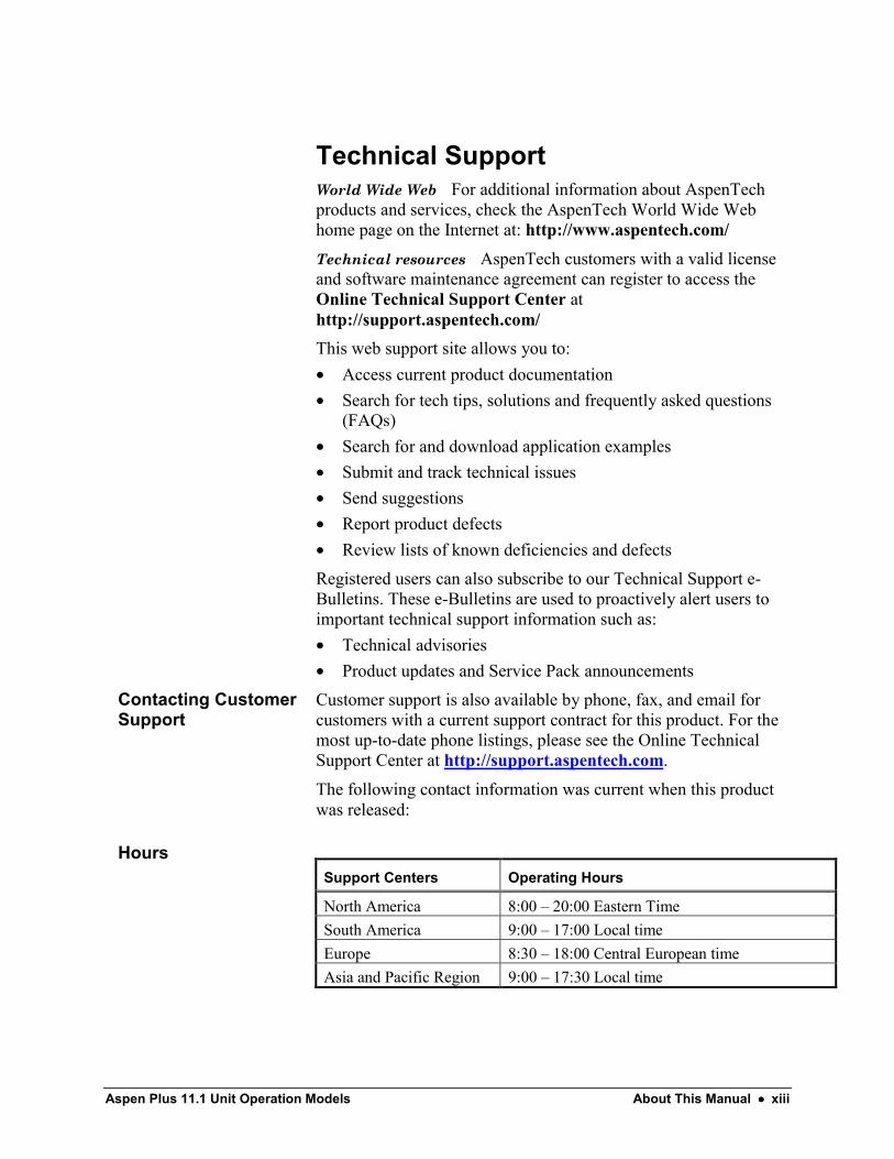
Technical SupportWorld Wide Web For additional information about AspenTechproducts and services, check the AspenTech World Wide Webhome page on the Internet at: http://www.aspentech.com/Technical resources AspenTech customers with a valid licenseand software maintenance agreement can register to access theOnline Technical Support Center athttp://support.aspentech.com/This web support site allows you to:• Access current product documentation• Search for tech tips, solutions and frequently asked questions
(FAQs)• Search for and download application examples• Submit and track technical issues• Send suggestions• Report product defects• Review lists of known deficiencies and defectsRegistered users can also subscribe to our Technical Support e-Bulletins. These e-Bulletins are used to proactively alert users toimportant technical support information such as:• Technical advisories• Product updates and Service Pack announcementsCustomer support is also available by phone, fax, and email forcustomers with a current support contract for this product. For themost up-to-date phone listings, please see the Online TechnicalSupport Center at http://support.aspentech.com.
The following contact information was current when this productwas released:
Support Centers Operating Hours
North America 8:00 – 20:00 Eastern TimeSouth America 9:00 – 17:00 Local timeEurope 8:30 – 18:00 Central European timeAsia and Pacific Region 9:00 – 17:30 Local time
Contacting CustomerSupport
Hours

xiv •••• About This Manual Aspen Plus 11.1 Unit Operation Models
SupportCenters
Phone Numbers
1-888-996-7100 Toll-free from U.S., Canada, Mexico1-281-584-4357 North America Support Center
NorthAmerica
(52) (5) 536-2809 Mexico Support Center(54) (11) 4361-7220 Argentina Support Center(55) (11) 5012-0321 Brazil Support Center(0800) 333-0125 Toll-free to U.S. from Argentina(000) (814) 550-4084 Toll-free to U.S. from Brazil
SouthAmerica
8001-2410 Toll-free to U.S. from Venezuela(32) (2) 701-95-55 European Support CenterCountry specific toll-free numbers:Belgium (0800) 40-687Denmark 8088-3652Finland (0) (800) 1-19127France (0805) 11-0054Ireland (1) (800) 930-024Netherlands (0800) 023-2511Norway (800) 13817Spain (900) 951846Sweden (0200) 895-284Switzerland (0800) 111-470
Europe
UK (0800) 376-7903(65) 395-39-00 SingaporeAsia and
PacificRegion
(81) (3) 3262-1743 Tokyo
Phone

Aspen Plus 11.1 Unit Operation Models About This Manual •••• xv
Support Centers Fax Numbers
North America 1-617-949-1724 (Cambridge, MA)1-281-584-1807 (Houston, TX: both Engineering andManufacturing Suite)1-281-584-5442 (Houston, TX: eSupply Chain Suite)1-281-584-4329 (Houston, TX: Advanced Control Suite)1-301-424-4647 (Rockville, MD)1-908-516-9550 (New Providence, NJ)1-425-492-2388 (Seattle, WA)
South America (54) (11) 4361-7220 (Argentina)(55) (11) 5012-4442 (Brazil)
Europe (32) (2) 701-94-45Asia and PacificRegion
(65) 395-39-50 (Singapore)(81) (3) 3262-1744 (Tokyo)
Support Centers E-mail
North America [email protected] (Engineering Suite)[email protected] (Aspen ICARUS products)[email protected] (Aspen MIMI products)[email protected] (Aspen PIMS products)[email protected] (Aspen Retail products)[email protected] (Advanced Control products)[email protected] (Manufacturing Suite)[email protected] (Mexico)
South America [email protected] (Argentina)[email protected] (Brazil)
Europe [email protected] (Engineering Suite)[email protected] (All other suites)[email protected] (CIMVIEW products)
Asia and PacificRegion
[email protected] (Singapore: Engineering Suite)[email protected] (Singapore: All other suites)[email protected] (Tokyo: Engineering Suite)[email protected] (Tokyo: All other suites)
Fax

xvi •••• About This Manual Aspen Plus 11.1 Unit Operation Models
Aspen Plus 11.1 Unit Operation Models Mixers and Splitters • 1-1
C H A P T E R 1
Mixers and Splitters
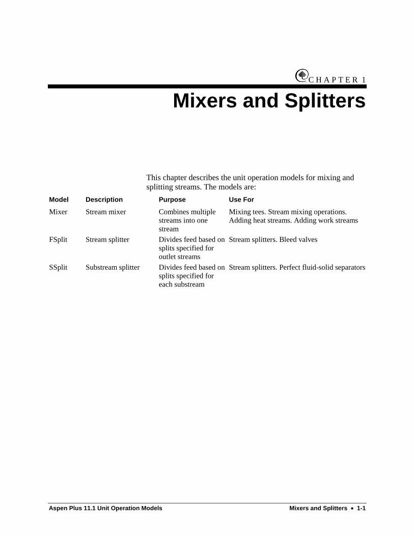
This chapter describes the unit operation models for mixing andsplitting streams. The models are:
Model Description Purpose Use For
Mixer Stream mixer Combines multiplestreams into onestream
Mixing tees. Stream mixing operations.Adding heat streams. Adding work streams
FSplit Stream splitter Divides feed based onsplits specified foroutlet streams
Stream splitters. Bleed valves
SSplit Substream splitter Divides feed based onsplits specified foreach substream
Stream splitters. Perfect fluid-solid separators

1-2 • Mixers and Splitters Aspen Plus 11.1 Unit Operation Models
Mixer ReferenceUse Mixer to combine streams into one stream. Mixer modelsmixing tees or other types of mixing operations.
Mixer combines material streams (or heat streams or workstreams) into one stream. Select the Heat (Q) and Work (W) Mixericons from the Model Library for heat and work streamsrespectively. A single Mixer block cannot mix streams of differenttypes (material, heat, work).
Use the following forms to enter specifications and view results forMixer:
Use this form To do this
Input Enter operating conditions and flash convergenceparameters
Block Options Override global values for physical properties,simulation options, diagnostic message levels, andreport options for this block
Results View Mixer simulation results
Dynamic Specify parameters for dynamic simulations
Material
Water (optional)
Material(2 or more)
Flowsheet for Mixing Material Streams
Material Streams
inlet At least two material streams
outlet One material streamOne water decant stream (optional)
HeatHeat
(2 or more)
Flowsheet for Adding Heat Streams
FlowsheetConnectivity forMixer

Aspen Plus 11.1 Unit Operation Models Mixers and Splitters • 1-3
Heat Streams
inlet At least two heat streams
outlet One heat stream
WorkWork
(2 or more)
Flowsheet for Adding Work Streams
Work Streams
inlet At least two work streams
outlet One work stream
Use the Mixer Input Flash Options sheet to specify operatingconditions.
When mixing heat or work streams, Mixer does not require anyspecifications.
When mixing material streams, you can specify either the outletpressure or pressure drop. If you specify pressure drop, Mixerdetermines the minimum of the inlet stream pressures, and appliesthe pressure drop to the minimum inlet stream pressure to computethe outlet pressure. If you do not specify the outlet pressure orpressure drop, Mixer uses the minimum pressure from the inletstreams for the outlet pressure.
You can select the following valid phases:
Valid Phase Solids? Number ofphases?
FreeWater?
Phase?
Vapor-Only Yes or no 1 No V
Liquid-Only Yes or no 1 No L
Vapor-Liquid Yes or no 2 No –
Vapor-Liquid-Liquid Yes or no 3 No –
Liquid Free-Water † Yes or no 1 Yes –
Vapor-Liquid Free-Water † Yes or no 2 Yes –
Solid-Only Yes 1 No S
† Check the Use Free Water Calculations checkbox on the SetupSpecifications Global sheet.
An optional water decant stream can be used when free-watercalculations are performed.
Specifying Mixer

1-4 • Mixers and Splitters Aspen Plus 11.1 Unit Operation Models
Mixer performs an adiabatic calculation on the product todetermine the outlet temperature, unless Mass Balance OnlyCalculations is specified on the Mixer BlockOptionsSimulationOptions sheet or the Setup SimulationOptionsCalculations sheet.
All features of Mixer are available in the EO formulation, exceptthe features which are globally unsupported.
EO Usage Notes forMixer
Aspen Plus 11.1 Unit Operation Models Mixers and Splitters • 1-5
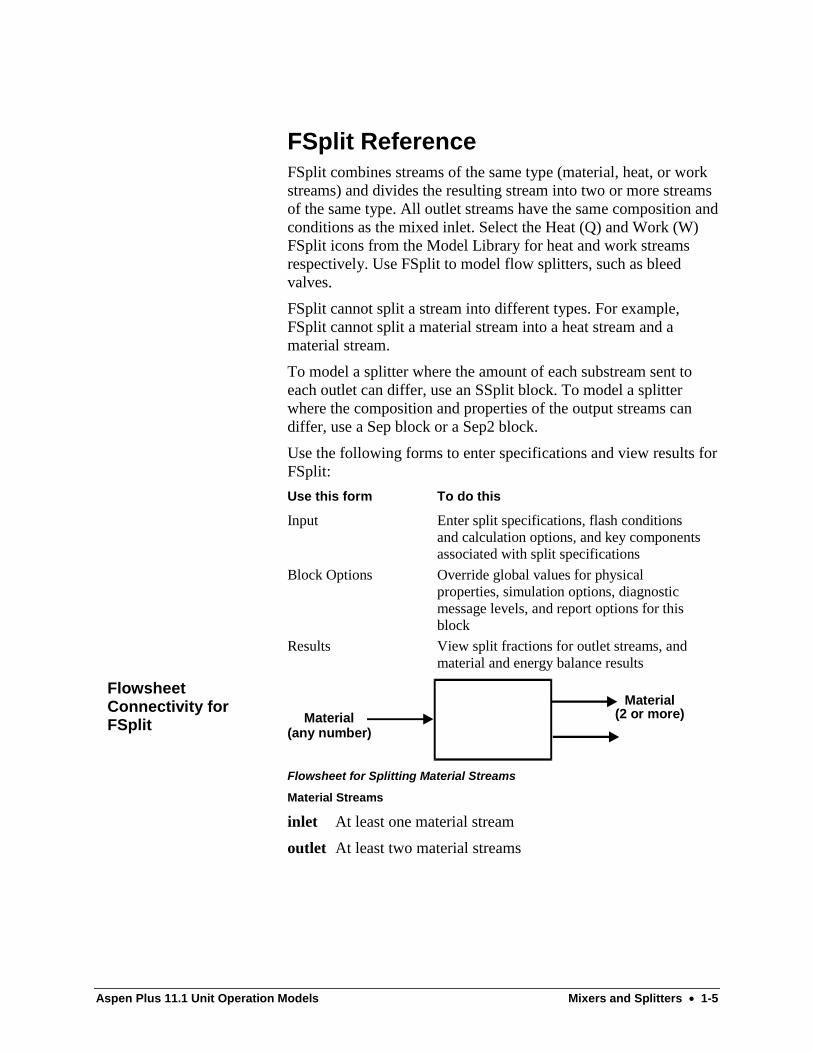
FSplit ReferenceFSplit combines streams of the same type (material, heat, or workstreams) and divides the resulting stream into two or more streamsof the same type. All outlet streams have the same composition andconditions as the mixed inlet. Select the Heat (Q) and Work (W)FSplit icons from the Model Library for heat and work streamsrespectively. Use FSplit to model flow splitters, such as bleedvalves.
FSplit cannot split a stream into different types. For example,FSplit cannot split a material stream into a heat stream and amaterial stream.
To model a splitter where the amount of each substream sent toeach outlet can differ, use an SSplit block. To model a splitterwhere the composition and properties of the output streams candiffer, use a Sep block or a Sep2 block.
Use the following forms to enter specifications and view results forFSplit:
Use this form To do this
Input Enter split specifications, flash conditionsand calculation options, and key componentsassociated with split specifications
Block Options Override global values for physicalproperties, simulation options, diagnosticmessage levels, and report options for thisblock
Results View split fractions for outlet streams, andmaterial and energy balance results
Material(2 or more)Material
(any number)
Flowsheet for Splitting Material Streams
Material Streams
inlet At least one material stream
outlet At least two material streams
FlowsheetConnectivity forFSplit

1-6 • Mixers and Splitters Aspen Plus 11.1 Unit Operation Models
Heat(2 or more)Heat
(any number)
Flowsheet for Splitting Heat Streams
Heat Streams
inlet At least one heat stream
outlet At least two heat streams
Work(2 or more)Work
(any number)
Flowsheet for Splitting Work Streams
Work Streams
inlet At least one work stream
outlet At least two work streams
To split material streams Give one of the following specificationsfor each outlet stream except one:
• Fraction of the combined inlet flow
• Mole flow rate
• Mass flow rate
• Standard liquid volume flow rate
• Actual volume flow rate
• Fraction of the residue remaining after all other specificationsare satisfied
FSplit puts any remaining flow in the unspecified outlet stream tosatisfy material balance. You can specify mole, mass, or standardliquid volume flow rate for one of the following:
• The entire stream
• A subset of key components in the stream
To specify the flow rate of a component or group of components inan outlet stream, specify a group of key components and the totalflow rate for the group (the sum of the component flow rates) onthe Input Specifications sheet, and define the key components inthe group on the Input KeyComponents sheet.
Outlet streams have the same composition as the mixed inletstream. For this reason, when you specify the flow rate of a keycomponent, the total flow rate of the outlet stream is greater thanthe flow rate you specify.
Specifying FSplit

Aspen Plus 11.1 Unit Operation Models Mixers and Splitters • 1-7
When FSplit has more than one inlet, you can do one of thefollowing:
• Enter the outlet pressure on the FSplit Input FlashOptions sheet
• Let the outlet pressure default to the minimum pressure of theinlet streams
To split heat streams or work streams Specify the fraction of thecombined inlet heat or work for each outlet stream except one.FSplit puts any remaining heat or work in the unspecified outletstream to satisfy energy balance.
The features listed below are not supported in equation-orientedformulation. However, the capabilities are still available for the EOsolution strategy via the Perturbation Layer.
• Specifications which result in renormalized split fractionsduring sequential-modular calculations
• Features which are globally unsupported
EO Usage Notes forFSplit

1-8 • Mixers and Splitters Aspen Plus 11.1 Unit Operation Models
SSplit ReferenceSSplit combines material streams and divides the resulting streaminto two or more streams. Use SSplit to model a splitter where thesplit of each substream among the outlet streams can differ.
Substreams in the outlet streams have the same composition,temperature, and pressure as the corresponding substreams in themixed inlet stream. Only the substream flow rates differ. To modela splitter in which the composition and properties of thesubstreams in the output streams can differ, use a Sep block or aSep2 block.
Use the following forms to enter specifications and view results forSSplit:
Use this form To do this
Input Enter split specifications, flash conditions,calculation options, and key components associatedwith split specifications
BlockOptions Override global values for physical properties,simulation options, diagnostic message levels, andreport options for this block
Results View split fractions of each substream in each outletstream, and material and energy balance results
Material(2 or more)Material
(any number)
Material Streams
inlet At least one material stream
outlet At least two material streams
For each substream, specify one of the following for all but oneoutlet stream:
• Fraction of the inlet substream
• Mole flow rate
• Mass flow rate
• Standard liquid volume flow rate
SSplit puts any remaining flow for each substream in theunspecified stream. You cannot specify standard liquid volumeflow rate when the substream is of type CISOLID, and mole andstandard liquid volume flow rates when the substream is of typeNC.
FlowsheetConnectivity forSSplit
Specifying SSplit

Aspen Plus 11.1 Unit Operation Models Mixers and Splitters • 1-9
You can specify mole or mass flow rate for one of the following:
• The entire substream
• A subset of components in the substream
You can specify the flow rate of a component in a substream of anoutlet stream. To do this, define a key component and specify theflow rate for the key component. Similarly, you can specify theflow rate for a group of components in a substream of an outletstream. To do this, define a key group of components and specifythe total flow rate for the group (the sum of the component flowrates).
Substreams in outlet streams have the same composition as thecorresponding substream in the mixed inlet stream. For this reason,when you specify the flow rate of a key, the total flow rate of thesubstream in the outlet stream is greater than the flow rate youspecify.
When SSplit has more than one inlet, you can do one of thefollowing:
• Enter the outlet pressure on the Input FlashOptions sheet.
• Let the outlet pressure default to the minimum pressure of theinlet streams.
The composition, temperature, pressure, and other substreamvariables for all outlet streams have the same values as the mixedinlet. Only the substream flow rates differ.

1-10 • Mixers and Splitters Aspen Plus 11.1 Unit Operation Models

Aspen Plus 11.1 Unit Operation Models Separators • 2-1
C H A P T E R 2
Separators
This chapter describes the unit operation models for componentseparators, flash drums, and liquid-liquid separators. The modelsare:
Model Description Purpose Use For
Flash2 Two-outlet flash Separates feed into twooutlet streams, usingrigorous vapor-liquid orvapor-liquid-liquidequilibrium
Flash drums, evaporators, knock-out drums,single stage separators
Flash3 Three-outlet flash Separates feed into threeoutlet streams, usingrigorous vapor-liquid-liquid equilibrium
Decanters, single-stage separators with twoliquid phases
Decanter Liquid-liquid decanter Separates feed into twoliquid outlet streams
Decanters, single-stage separators with twoliquid phases and no vapor phase
Sep Component separator Separates inlet streamcomponents intomultiple outlet streams,based on specified flowsor split frractions
Component separation operations, such asdistillation and absorption, when the detailsof the separation are unknown orunimportant
Sep2 Two-outlet componentseparator
Separates inlet streamcomponents into twooutlet streams, based onspecified flows, splitfractions, or purities
Component separation operations, such asdistillation and absorption, when the detailsof the separation are unknown orunimportant
You can generate heating or cooling curve tables for Flash2,Flash3, and Decanter models.

2-2 • Separators Aspen Plus 11.1 Unit Operation Models
Flash2 ReferenceUse Flash2 to model flashes, evaporators, knock-out drums, andother single-stage separators. Flash2 performs vapor-liquid orvapor-liquid-liquid equilibrium calculations. When you specify theoutlet conditions, Flash2 determines the thermal and phaseconditions of a mixture of one or more inlet streams.
Use the following forms to enter specifications and view results forFlash2.
Use this form To do this
Input Enter flash specifications, flash convergenceparameters, and entrainment specifications
Hcurves Specify heating or cooling curve tables and viewtabular results
Block Options Override global values for physical properties,simulation options, diagnostic message levels, andreport options for this block
Results View Flash2 simulation results
Dynamic Specify parameters for dynamic simulations
Vapor
Liquid
Water (optional)
Heat (optional)
Heat(optional)
Material(any number)
Material Streams
inlet At least one material stream
outlet One material stream for the vapor phaseOne material stream for the liquid phase. (If three phasesexist, the liquid outlet contains both liquid phases.)One water decant stream (optional)
You can specify liquid and/or solid entrainment in the vaporstream.
FlowsheetConnectivity forFlash2
Aspen Plus 11.1 Unit Operation Models Separators • 2-3
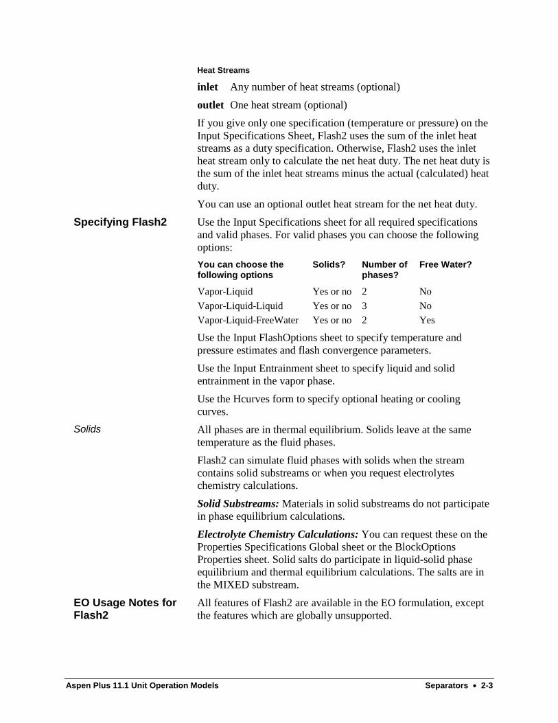
Heat Streams
inlet Any number of heat streams (optional)
outlet One heat stream (optional)
If you give only one specification (temperature or pressure) on theInput Specifications Sheet, Flash2 uses the sum of the inlet heatstreams as a duty specification. Otherwise, Flash2 uses the inletheat stream only to calculate the net heat duty. The net heat duty isthe sum of the inlet heat streams minus the actual (calculated) heatduty.
You can use an optional outlet heat stream for the net heat duty.
Use the Input Specifications sheet for all required specificationsand valid phases. For valid phases you can choose the followingoptions:
You can choose thefollowing options
Solids? Number ofphases?
Free Water?
Vapor-Liquid Yes or no 2 No
Vapor-Liquid-Liquid Yes or no 3 No
Vapor-Liquid-FreeWater Yes or no 2 Yes
Use the Input FlashOptions sheet to specify temperature andpressure estimates and flash convergence parameters.
Use the Input Entrainment sheet to specify liquid and solidentrainment in the vapor phase.
Use the Hcurves form to specify optional heating or coolingcurves.
All phases are in thermal equilibrium. Solids leave at the sametemperature as the fluid phases.
Flash2 can simulate fluid phases with solids when the streamcontains solid substreams or when you request electrolyteschemistry calculations.
Solid Substreams: Materials in solid substreams do not participatein phase equilibrium calculations.
Electrolyte Chemistry Calculations: You can request these on theProperties Specifications Global sheet or the BlockOptionsProperties sheet. Solid salts do participate in liquid-solid phaseequilibrium and thermal equilibrium calculations. The salts are inthe MIXED substream.
All features of Flash2 are available in the EO formulation, exceptthe features which are globally unsupported.
Specifying Flash2
Solids
EO Usage Notes forFlash2

2-4 • Separators Aspen Plus 11.1 Unit Operation Models
Flash3 ReferenceUse Flash3 to model flashes, evaporators, knock-out drums,decanters, and other single-stage separators in which two liquidoutlet streams are produced. Flash3 performs vapor-liquid-liquidequilibrium calculations. When you specify outlet conditions,Flash3 determines the thermal and phase conditions of a mixture ofone or more inlet streams.
Use the following forms to enter specifications and view results forFlash3:
Use this form To do this
Input Enter flash specifications, key components, flashconvergence parameters, and entrainmentspecifications
Hcurves Specify heating or cooling curve tables and viewtabular results
Block Options Override global values for physical properties,simulation options, diagnostic message levels,and report options for this block
Results View Flash3 simulation results
Dynamic Specify parameters for dynamic simulations
Vapor
2nd Liquid
1st Liquid
Heat (optional)
Heat(optional)
Material(any number)
Material Streams
inlet At least one material stream
outlet One material stream for the vapor phaseOne material stream for the first liquid phaseOne material stream for the second liquid phase
FlowsheetConnectivity forFlash3

Aspen Plus 11.1 Unit Operation Models Separators • 2-5
You can specify liquid entrainment of each liquid phase in thevapor stream. You can also specify entrainment for each solidsubstream in the vapor and first liquid phase.
Heat Streams
inlet Any number of heat streams (optional)
outlet One heat stream (optional)
If you give only one specification on the Input Specifications Sheet(temperature or pressure), Flash3 uses the sum of the inlet heatstreams as a duty specification. Otherwise, Flash3 uses the inletheat stream only to calculate the net heat duty. The net heat duty isthe sum of the inlet heat streams minus the actual (calculated) heatduty.
You can use an optional outlet heat stream for the net heat duty.
Use the Input Specifications sheet for all required specifications.
Use the Input Entrainment sheet to specify solid entrainment.
To specify optional heating or cooling curves, use the Hcurvesform.
All phases are in thermal equilibrium. Solids leave at the sametemperature as the fluid phases.
Flash3 can simulate fluid phases with solids when the streamcontains solid substreams, or when you request electrolytechemistry calculations.
Solid Substreams: Materials in solid substreams do not participatein phase equilibrium calculations.
Electrolyte Chemistry Calculations: You can request these on theProperties Specifications Global sheet or on the InputBlockOptions Properties sheet. Solid salts do participate in liquid-solid phase equilibrium and thermal equilibrium calculations. Youcan only specify apparent component calculations (SelectSimulation Approach=Apparent Components on the BlockOptionsProperties sheet). The salts will not appear in the MIXEDsubstream.
Specifying Flash3
Solids

2-6 • Separators Aspen Plus 11.1 Unit Operation Models
Decanter ReferenceDecanter simulates decanters and other single stage separatorswithout a vapor phase. Decanter can perform:
• Liquid-liquid equilibrium calculations
• Liquid-free-water calculations
Use Decanter to model knock-out drums, decanters, and othersingle-stage separators without a vapor phase. When you specifyoutlet conditions, Decanter determines the thermal and phaseconditions of a mixture of one or more inlet streams.
Decanter can calculate liquid-liquid distribution coefficients using:
• An activity coefficient model
• An equation of state capable of representing two liquid phases
• A user-specified Fortran subroutine
• A built-in correlation with user-specified coefficients
You can enter component separation efficiencies, assumingequilibrium stage is present.
Use Flash3 if you suspect any vapor phase formation.
Use the following forms to enter specifications and view results forDecanter:
Use this form To do this
Input Specify operating conditions, key components,calculation options, valid phases, efficiency, andentrainment
Properties Specify and/or override property methods, KLLequation parameters, and/or user subroutine forphase split calculations
Hcurves Specify heating or cooling curve tables and viewtabular results
Block Options Override global values for physical properties,simulation options, diagnostic message levels,and report options for this block
Results Display simulation results
Dynamic Specify parameters for dynamic simulations
Heat(optional)
Heat(optional)
1st Liquid
2nd Liquid
Material(any number)
FlowsheetConnectivity forDecanter

Aspen Plus 11.1 Unit Operation Models Separators • 2-7
Material Streams
inlet At least one material stream
outlet One material stream for the first liquid phaseOne material stream for the second liquid phase
You can specify entrainment for each solid substream in the firstliquid phase.
Heat Streams
inlet Any number of heat streams (optional)
outlet One heat stream (optional)
If you specify only pressure on the Input Specifications sheet,Decanter uses the sum of the inlet heat streams as a dutyspecification. Otherwise, Decanter uses the inlet heat stream onlyto calculate the net heat duty. The net heat duty is the sum of theinlet heat streams minus the actual (calculated) heat duty.
You can use an optional outlet heat stream for the net heat duty.
You can operate Decanter in one of the following ways:
• Adiabatically
• With specified duty
• At a specified temperature
Use the Input Specifications sheet to enter:
• Pressure
• Temperature or duty
If two liquid phases are present at the decanter operating condition,Decanter treats the phase with higher density as the second phase,by default.
When only one liquid phase exists and you want to avoidambiguities, you can override the default by:
• Specifying key components for identifying the second liquidphase on the Input Specifications sheet
• Optionally specifying the threshold key component molefraction on the Input Specifications sheet
When Decanter treats the
Two liquid phases arepresent
Phase with the higher mole fraction of keycomponents as the second liquid phase
One liquid phase ispresent
Liquid phase as the first liquid phase, unless themole fraction of key components exceeds thethreshold value
Specifying Decanter
Defining the SecondLiquid Phase
2-8 • Separators Aspen Plus 11.1 Unit Operation Models
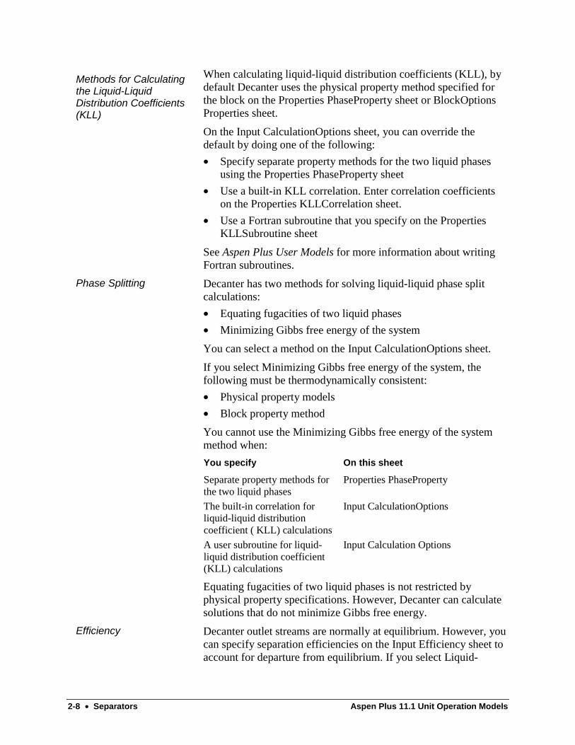
When calculating liquid-liquid distribution coefficients (KLL), bydefault Decanter uses the physical property method specified forthe block on the Properties PhaseProperty sheet or BlockOptionsProperties sheet.
On the Input CalculationOptions sheet, you can override thedefault by doing one of the following:
• Specify separate property methods for the two liquid phasesusing the Properties PhaseProperty sheet
• Use a built-in KLL correlation. Enter correlation coefficientson the Properties KLLCorrelation sheet.
• Use a Fortran subroutine that you specify on the PropertiesKLLSubroutine sheet
See Aspen Plus User Models for more information about writingFortran subroutines.
Decanter has two methods for solving liquid-liquid phase splitcalculations:
• Equating fugacities of two liquid phases
• Minimizing Gibbs free energy of the system
You can select a method on the Input CalculationOptions sheet.
If you select Minimizing Gibbs free energy of the system, thefollowing must be thermodynamically consistent:
• Physical property models
• Block property method
You cannot use the Minimizing Gibbs free energy of the systemmethod when:
You specify On this sheet
Separate property methods forthe two liquid phases
Properties PhaseProperty
The built-in correlation forliquid-liquid distributioncoefficient ( KLL) calculations
Input CalculationOptions
A user subroutine for liquid-liquid distribution coefficient(KLL) calculations
Input Calculation Options
Equating fugacities of two liquid phases is not restricted byphysical property specifications. However, Decanter can calculatesolutions that do not minimize Gibbs free energy.
Decanter outlet streams are normally at equilibrium. However, youcan specify separation efficiencies on the Input Efficiency sheet toaccount for departure from equilibrium. If you select Liquid-
Methods for Calculatingthe Liquid-LiquidDistribution Coefficients(KLL)
Phase Splitting
Efficiency

Aspen Plus 11.1 Unit Operation Models Separators • 2-9
FreeWater for Valid Phases on the Input CalculationOptions sheet,you cannot specify separation efficiencies.
If solids substreams are present, they do not participate in phaseequilibrium calculations, but they do participate in enthalpybalance. You can use the Input Entrainment sheet to specify solidsentrainment in the first liquid outlet stream. Decanter places anyremaining solids in the second liquid outlet stream.
The features listed below are not supported in equation-orientedformulation. However, the capabilities are still available for the EOsolution strategy via the Perturbation Layer.
• User KLL subroutine
• KLL correlation
• Features which are globally unsupported
Solids Entrainment
EO Usage Notes forDecanter

2-10 • Separators Aspen Plus 11.1 Unit Operation Models
Sep ReferenceSep combines streams and separates the result into two or morestreams according to splits specified for each component. Whenthe details of the separation are unknown or unimportant, but thesplits for each component are known, you can use Sep in place of arigorous separation model to save computation time .
If the composition and conditions of all outlet streams of the blockyou are modeling are identical, you can use an FSplit block insteadof Sep.
Use the following forms to enter specifications and view results forSep:
Use this form To do this
Input Enter split specifications, flash specifications, andconvergence parameters for the mixed inlet and eachoutlet stream
Block Options Override global values for physical properties,simulation options, diagnostic message levels, andreport options for this block
Results View Sep simulation results
Heat(optional)
Material(2 or more)
Material(any number)
Material Streams
inlet At least one material stream
outlet At least two material streams
Heat Streams
inlet No inlet heat streams
outlet One stream for the enthalpy difference between inlet andoutlet material streams (optional)
For each substream of each outlet stream except one, use the SepInput Specifications sheet to specify one of the following for eachcomponent present:
• Fraction of the component in the corresponding inlet substream
• Mole flow rate of the component
• Mass flow rate of the component
• Standard liquid volume flow rate of the component
FlowsheetConnectivity for Sep
Specifying Sep
Aspen Plus 11.1 Unit Operation Models Separators • 2-11
Sep puts any remaining flow in the corresponding substream of theunspecified outlet stream.
Use the Sep Input Feed Flash sheet to specify either the pressuredrop or the pressure at the inlet. This is useful when Sep has morethan one inlet stream. The inlet pressure defaults to the minimuminlet stream pressure.
Use the Sep Input Outlet Flash sheet to specify the conditions ofthe outlet streams. If you do not specify the conditions for astream, Sep uses the inlet temperature and pressure.
The features listed below are not supported in equation-orientedformulation. However, the capabilities are still available for the EOsolution strategy via the Perturbation Layer.
• Specifications which result in renormalized split fractionsduring sequential-modular calculations
• Features which are globally unsupported
Inlet Pressure
Outlet Stream Conditions
EO Usage Notes forSep

2-12 • Separators Aspen Plus 11.1 Unit Operation Models
Sep2 ReferenceSep2 separates inlet stream components into two outlet streams.Sep2 is similar to Sep, but offers a wider variety of specifications.Sep2 allows purity (mole-fraction) specifications for components.
You can use Sep2 in place of a rigorous separation model, such asdistillation or absorption. Sep2 saves computation time whendetails of the separation are unknown or unimportant.
If the composition and conditions of all outlet streams of the blockyou are modeling are identical, you can use FSplit instead of Sep2.
Use the following forms to enter specifications and view results forSep2:
Use this form To do this
Input Enter split specifications, flash specifications, andconvergence parameters for the mixed inlet and eachoutlet stream
Block Options Override global values for physical properties,simulation options, diagnostic message levels, andreport options for this block
Results View Sep2 simulation results
Material
Material
Heat(optional)
Material(any number)
Material Streams
inlet At least one material stream
outlet Two material streams
Heat Streams
inlet No inlet heat streams
outlet One stream for the enthalpy difference between inlet andoutlet materialstreams (optional)
Use the Input Specifications sheet to specify stream and/orcomponent fractions and flows. The number of specifications foreach substream must equal the number of components in thatsubstream.
FlowsheetConnectivity for Sep2
Specifying Sep2

Aspen Plus 11.1 Unit Operation Models Separators • 2-13
You can enter these stream specifications:
• Fraction of the total inlet stream going to either outlet stream
• Total mass flow rate of an outlet stream
• Total molar flow rate of an outlet stream (for substreams oftype MIXED or CISOLID)
• Total standard liquid volume flow rate of an outlet stream (forsubstreams of type MIXED)
You can enter these component specifications:
• Fraction of a component in the feed going to either outletstream
• Mass flow rate of a component in an outlet stream
• Molar flow rate of a component in an outlet stream (forsubstreams of type MIXED or CISOLID)
• Standard liquid volume flow rate of a component in an outletstream (for substreams of type MIXED)
• Mass fraction of a component in an outlet stream
• Mole fraction of a component in an outlet stream (forsubstreams of type MIXED or CISOLID)
Sep2 treats each substream separately. Do not:
• Specify the total flow of both outlet streams
• Enter more than one flow or frac specification for eachcomponent
• Enter both a mole-frac and a mass-frac specification for acomponent in a stream
Use the Input Feed Flash sheet to specify either the pressure dropor pressure at the inlet. This information is useful when Sep2 hasmore than one inlet stream. The inlet pressure defaults to theminimum of the inlet stream pressures.
Use the Input Outlet Flash sheet to specify the conditions of theoutlet streams. If you do not specify the conditions for a stream,Sep2 uses the inlet temperature and pressure.
The features listed below are not supported in equation-orientedformulation. However, the capabilities are still available for the EOsolution strategy via the Perturbation Layer.
• Specifications which result in renormalized split fractionsduring sequential-modular calculations
• Features which are globally unsupported
Inlet Pressure
Outlet Stream Conditions
EO Usage Notes forSep2

2-14 • Separators Aspen Plus 11.1 Unit Operation Models
Aspen Plus 11.1 Unit Operation Models Heat Exchangers • 3-1
C H A P T E R 3
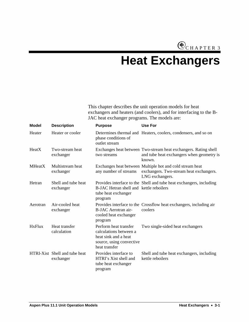
Heat Exchangers
This chapter describes the unit operation models for heatexchangers and heaters (and coolers), and for interfacing to the B-JAC heat exchanger programs. The models are:
Model Description Purpose Use For
Heater Heater or cooler Determines thermal andphase conditions ofoutlet stream
Heaters, coolers, condensers, and so on
HeatX Two-stream heatexchanger
Exchanges heat betweentwo streams
Two-stream heat exchangers. Rating shelland tube heat exchangers when geometry isknown.
MHeatX Multistream heatexchanger
Exchanges heat betweenany number of streams
Multiple hot and cold stream heatexchangers. Two-stream heat exchangers.LNG exchangers.
Hetran Shell and tube heatexchanger
Provides interface to theB-JAC Hetran shell andtube heat exchangerprogram
Shell and tube heat exchangers, includingkettle reboilers
Aerotran Air-cooled heatexchanger
Provides interface to theB-JAC Aerotran air-cooled heat exchangerprogram
Crossflow heat exchangers, including aircoolers
HxFlux Heat transfercalculation
Perform heat transfercalculations between aheat sink and a heatsource, using convectiveheat transfer
Two single-sided heat exchangers
HTRI-Xist Shell and tube heatexchanger
Provides interface toHTRI’s Xist shell andtube heat exchangerprogram
Shell and tube heat exchangers, includingkettle reboilers

3-2 • Heat Exchangers Aspen Plus 11.1 Unit Operation Models
Heater ReferenceYou can use Heater to represent:
• Heaters
• Coolers
• Valves
• Pumps (whenever work-related results are not needed)
• Compressors (whenever work-related results are not needed)
You also can use Heater to set the thermodynamic condition of astream.
When you specify the outlet conditions, Heater determines thethermal and phase conditions of a mixture with one or more inletstreams.
Use the following forms to enter specifications and view results forHeater:
Use this form To do this
Input Enter operating conditions and flash convergenceparameters
Hcurves Specify heating or cooling curve tables and viewtabular results
Block Options Override global values for physical properties,simulation options, diagnostic message levels,and report options for this block
Results View Heater results
Heat (optional)
MaterialMaterial(any number)
Heat(optional)
Water (optional)
Material Streams
inlet At least one material stream
outlet One material streamOne water decant stream (optional)
Heat Streams
inlet Any number of heat streams (optional)
outlet One heat stream (optional)
FlowsheetConnectivity forHeater
Aspen Plus 11.1 Unit Operation Models Heat Exchangers • 3-3
If you give only one specification (temperature or pressure) on theSpecifications sheet, Heater uses the sum of the inlet heat streamsas a duty specification. Otherwise, Heater uses the inlet heat streamonly to calculate the net heat duty. The net heat duty is the sum ofthe inlet heat streams minus the actual (calculated) heat duty.
You can use an optional outlet heat stream for the net heat duty.
Use the Heater Input Specifications sheet for all requiredspecifications and valid phases.
Dew point calculations are two- or three-phase flashes with a vaporfraction of unity.
Bubble point calculations are two- or three-phase flashes with avapor fraction of zero.
Use the Heater Input FlashOptions sheet to specify temperatureand pressure estimates and flash convergence parameters.
Use the Hcurves form to specify optional heating or coolingcurves.
This model has no dynamic features. The pressure drop is fixed atthe steady state value. The outlet flow is determined by the massbalance.
Heater can simulate fluid phases with solids when the streamcontains solid substreams or when you request electrolytechemistry calculations.
All phases are in thermal equilibrium. Solids leave at the sametemperature as fluid phases.
Solid Substreams Materials in solid substreams do not participatein phase equilibrium calculations.
Electrolyte Chemistry Calculations You can request these on theProperties Specifications Global sheet or the Heater BlockOptionsProperties sheet. Solid salts participate in liquid-solid phaseequilibrium and thermal equilibrium calculations. The salts are inthe MIXED substream.
All features of Heater are available in the EO formulation, exceptthe features which are globally unsupported.
Specifying Heater
Solids
EO Usage Notes forHeater

3-4 • Heat Exchangers Aspen Plus 11.1 Unit Operation Models
HeatX ReferenceHeatX can model a wide variety of shell and tube heat exchangertypes including:
• Countercurrent and co-current
• Segmental baffle TEMA E, F, G, H, J, and X shells
• Rod baffle TEMA E and F shells
• Bare and low-finned tubes
HeatX can perform a full zone analysis with heat transfercoefficient and pressure drop estimation for single- and two-phasestreams. For rigorous heat transfer and pressure drop calculations,you must supply the exchanger geometry.
If exchanger geometry is unknown or unimportant, HeatX canperform simplified shortcut rating calculations. For example, youmay want to perform only heat and material balance calculations.
HeatX has correlations to estimate sensible heat, nucleate boiling,and condensation film coefficients.
HeatX can
• Perform design calculations
• Perform mechanical vibration analysis
• Estimate fouling factors
Use the following forms to enter specifications and view results forHeatX:
Use this form To do this
Setup Specify shortcut, detailed or Hetran-rigorouscalculations, flow direction, exchanger pressuredrops, heat transfer coefficient calculation methods,and film coefficients
Options Specify different flash convergence parameters andvalid phases for the hot and cold sides, HeatXconvergence parameters, and block-specific reportoption
Hetran Options Specify the name of the Hetran input file,parameters for calculating the property curves,optional Hetran program inputs.
Hetran Browser Specify data when using the Hetran-Rigorouscalculation type.
Geometry Specify the shell and tube configuration and indicateany tube fins, baffles, or nozzles

Aspen Plus 11.1 Unit Operation Models Heat Exchangers • 3-5
Use this form To do this
Hot-Hcurves Specify hot stream heating or cooling curve tablesand view tabular results
Cold-Hcurves Specify cold stream heating or cooling curve tablesand view tabular results
User Subroutines Specify parameters for user-defined Fortransubroutines to calculate overall heat transfercoefficient, LMTD correction factor, tube-sideliquid holdup, or tube-side pressure drop
Dynamic Specify parameters for dynamic simulations
Block Options Override global values for physical properties,simulation options, diagnostic message levels, andreport options for this block
Thermal Results View a summary of results, mass and energybalances, pressure drops, velocities, and zoneanalysis profiles
Geometry Results View detailed shell and tube results, and informationabout tube fins, baffles, and nozzles
Hetran ThermalResults
View overall results and detailed results for the shellside and tube side when using the Hetran-Rigorouscalculation type.
Cold Outlet
Water (optional)
Hot Outlet
Water(optional)
HotInlet
Cold InletMaterial Streams
inlet One hot inletOne cold inlet
outlet One hot outletOne cold outletOne water decant stream on the hot side (optional)One water decant stream on the cold side (optional)
FlowsheetConnectivity forHeatX
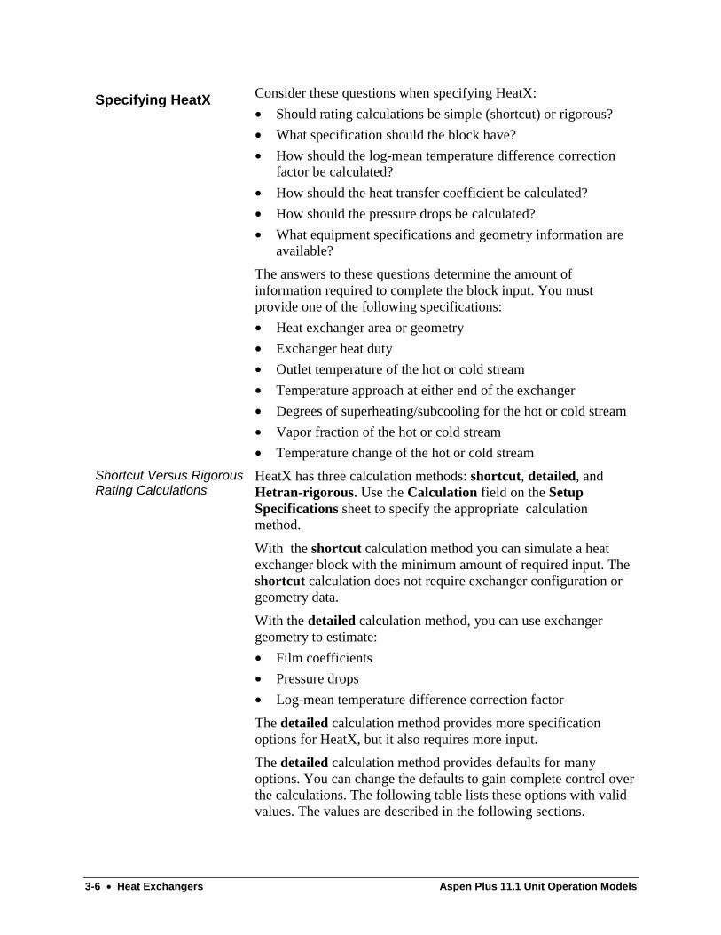
3-6 • Heat Exchangers Aspen Plus 11.1 Unit Operation Models
Consider these questions when specifying HeatX:
• Should rating calculations be simple (shortcut) or rigorous?
• What specification should the block have?
• How should the log-mean temperature difference correctionfactor be calculated?
• How should the heat transfer coefficient be calculated?
• How should the pressure drops be calculated?
• What equipment specifications and geometry information areavailable?
The answers to these questions determine the amount ofinformation required to complete the block input. You mustprovide one of the following specifications:
• Heat exchanger area or geometry
• Exchanger heat duty
• Outlet temperature of the hot or cold stream
• Temperature approach at either end of the exchanger
• Degrees of superheating/subcooling for the hot or cold stream
• Vapor fraction of the hot or cold stream
• Temperature change of the hot or cold stream
HeatX has three calculation methods: shortcut, detailed, andHetran-rigorous. Use the Calculation field on the SetupSpecifications sheet to specify the appropriate calculationmethod.
With the shortcut calculation method you can simulate a heatexchanger block with the minimum amount of required input. Theshortcut calculation does not require exchanger configuration orgeometry data.
With the detailed calculation method, you can use exchangergeometry to estimate:
• Film coefficients
• Pressure drops
• Log-mean temperature difference correction factor
The detailed calculation method provides more specificationoptions for HeatX, but it also requires more input.
The detailed calculation method provides defaults for manyoptions. You can change the defaults to gain complete control overthe calculations. The following table lists these options with validvalues. The values are described in the following sections.
Specifying HeatX
Shortcut Versus RigorousRating Calculations

Aspen Plus 11.1 Unit Operation Models Heat Exchangers • 3-7
The Hetran-rigorous method allows you to design newequipment, and to rate or simulate the performance of existingequipment. In addition to the more rigorous heat transfer andhydraulic analyses, the program will also determine possibleoperational problems such as vibration or excessive velocities. Youcan use the Hetran-rigorous method to estimate the cost for theequipment. The modules used in the Hetran-rigorous method arethe same as those used in the Aspen Hetran standalone product forshell and tube heat exchanger analysis.
Variable Calculation MethodAvailable inShortcut Mode
Available inDetailed Mode
Available inHetran-rigorous mode
LMTDCorrectionFactor
ConstantGeometryUser subroutineCalculated
Single tube pass †NoNoMultiple tube pass †
YesDefaultYesNo
NoNoNoNo
Heat TransferCoefficient
Constant valuePhase-specific valuesPower law expressionFilm coefficientsExchanger geometryUser subroutine
YesDefaultYesNoNoNo
YesYesYesYesDefaultYes
NoNoNoNoNoNo
FilmCoefficient
Constant valuePhase-specific valuesPower law expressionCalculate from geometry
NoNoNoNo
YesYesYesDefault
NoNoNoNo
Pressure Drop Outlet pressureCalculate from geometry
DefaultNo
YesDefault
NoNo
† In shortcut mode, a constant LMTD must be supplied forexchangers with a single tube pass. For exchangers with multipletube passes, the LMTD correction factor will be calculated.
The standard equation for a heat exchanger is:
Q U A LMTD= ⋅ ⋅
where LMTD is the log-mean temperature difference. Thisequation applies for exchangers with pure countercurrent flow.
The more general equation is:
Q U A F LMTD= ⋅ ⋅ ⋅
where the LMTD correction factor, F, accounts for deviation fromcountercurrent flow.
Use the LMTD Correction Factor field on the Setup Specificationssheet to enter the LMTD correction factor.
In shortcut rating mode, the LMTD correction factor is constant fora cocurrent or countercurrent exchanger. For a multipass
Calculating the Log-MeanTemperature DifferenceCorrection Factor
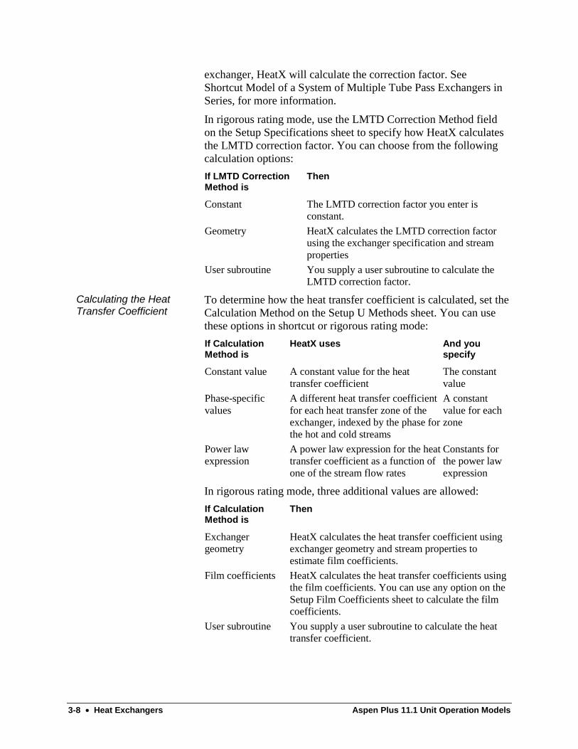
3-8 • Heat Exchangers Aspen Plus 11.1 Unit Operation Models
exchanger, HeatX will calculate the correction factor. SeeShortcut Model of a System of Multiple Tube Pass Exchangers inSeries, for more information.
In rigorous rating mode, use the LMTD Correction Method fieldon the Setup Specifications sheet to specify how HeatX calculatesthe LMTD correction factor. You can choose from the followingcalculation options:
If LMTD CorrectionMethod is
Then
Constant The LMTD correction factor you enter isconstant.
Geometry HeatX calculates the LMTD correction factorusing the exchanger specification and streamproperties
User subroutine You supply a user subroutine to calculate theLMTD correction factor.
To determine how the heat transfer coefficient is calculated, set theCalculation Method on the Setup U Methods sheet. You can usethese options in shortcut or rigorous rating mode:
If CalculationMethod is
HeatX uses And youspecify
Constant value A constant value for the heattransfer coefficient
The constantvalue
Phase-specificvalues
A different heat transfer coefficientfor each heat transfer zone of theexchanger, indexed by the phase forthe hot and cold streams
A constantvalue for eachzone
Power lawexpression
A power law expression for the heattransfer coefficient as a function ofone of the stream flow rates
Constants forthe power lawexpression
In rigorous rating mode, three additional values are allowed:
If CalculationMethod is
Then
Exchangergeometry
HeatX calculates the heat transfer coefficient usingexchanger geometry and stream properties toestimate film coefficients.
Film coefficients HeatX calculates the heat transfer coefficients usingthe film coefficients. You can use any option on theSetup Film Coefficients sheet to calculate the filmcoefficients.
User subroutine You supply a user subroutine to calculate the heattransfer coefficient.
Calculating the HeatTransfer Coefficient

Aspen Plus 11.1 Unit Operation Models Heat Exchangers • 3-9
HeatX does not calculate film coefficients in shortcut rating mode.In rigorous rating mode, if you use film coefficients or exchangergeometry for the heat transfer coefficient calculation method,HeatX calculates the heat transfer coefficient using:
1 1 1
U h hc h
= +
Where:
hc = Cold stream film coefficient
hh = Hot stream film coefficient
To choose an option for calculating film coefficients, set theCalculation Method on the Setup Film Coefficients sheet. Thefollowing are available:
If Calculation Method is HeatX uses And youspecify
Constant value A constant value for thefilm coefficient
A constantvalue to be usedthroughout theexchanger
Phase-specific values A different film coefficientfor each heat transfer zone(phase) of the exchanger,indexed by the phase of thestream
A constantvalue for eachphase
Power law expression A power law expression forthe film coefficient as afunction of the stream flowrate
Constants forthe power lawexpression
Calculate from geometry The exchanger geometryand stream properties tocalculate the filmcoefficient
The hot stream and cold stream film coefficient calculationmethods are independent of each other. You can use anycombination that is appropriate for your exchanger.
To enter exchanger pressure or pressure drop for the hot and coldsides, use the Outlet Pressure fields on the Setup Pressure Dropsheet. In shortcut rating mode the pressure drop is constant.
In rigorous rating mode, you can choose how pressure drops arecalculated by setting the pressure options on the SetupPressureDrop sheet. The following pressure drop options areavailable:
Film Coefficients
Pressure DropCalculations

3-10 • Heat Exchangers Aspen Plus 11.1 Unit Operation Models
If Pressure Option is Then
Outlet Pressure You must enter the outlet pressure or pressuredrop for the stream.
Calculate from geometry HeatX calculates the pressure drop using theexchanger geometry and stream properties
HeatX calls the Pipeline model to calculate tube-side pressuredrop. You can set the correlations for pressure drop and liquidholdup that the Pipeline model uses on the Setup PressureDropsheet.
Exchanger configuration refers to the overall patterns of flow inthe heat exchanger. If you choose Calculate From Geometry forany of the heat transfer coefficients, film coefficients, or pressuredrop calculation methods, you may be required to enter someinformation about the exchanger configuration on the GeometryShell sheet. This sheet includes fields for:
• TEMA shell type (see the next figure, TEMA Shell Types)
• Number of tube passes
• Exchanger orientation
• Tubes in baffle window
• Number of sealing strips
• Tube flow for vertical exchangers
Exchanger Configuration
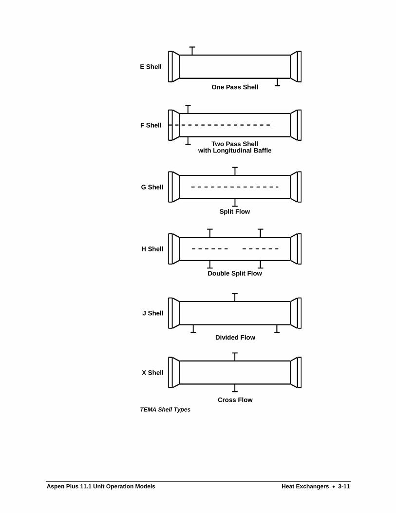
Aspen Plus 11.1 Unit Operation Models Heat Exchangers • 3-11
Two Pass Shellwith Longitudinal Baffle
One Pass Shell
E Shell
F Shell
G Shell
H Shell
J Shell
X Shell
Split Flow
Double Split Flow
Divided Flow
Cross FlowTEMA Shell Types
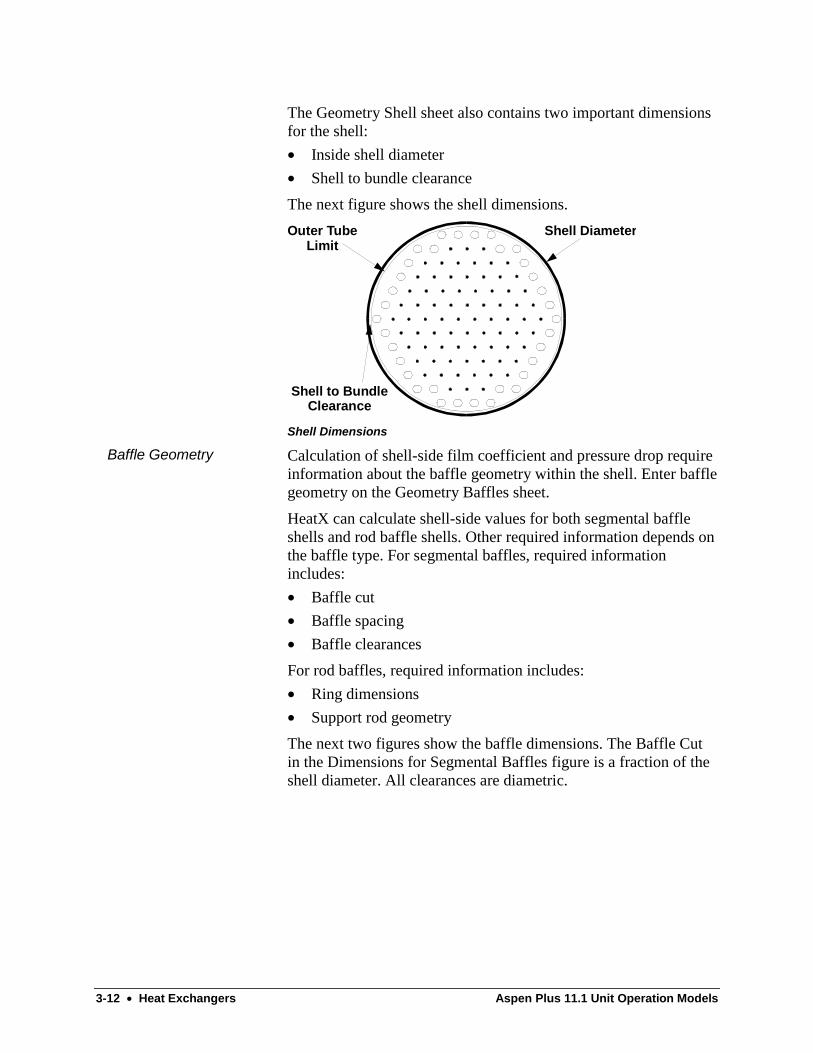
3-12 • Heat Exchangers Aspen Plus 11.1 Unit Operation Models
The Geometry Shell sheet also contains two important dimensionsfor the shell:
• Inside shell diameter
• Shell to bundle clearance
The next figure shows the shell dimensions.
Outer TubeLimit
Shell to BundleClearance
Shell Diameter
Shell Dimensions
Calculation of shell-side film coefficient and pressure drop requireinformation about the baffle geometry within the shell. Enter bafflegeometry on the Geometry Baffles sheet.
HeatX can calculate shell-side values for both segmental baffleshells and rod baffle shells. Other required information depends onthe baffle type. For segmental baffles, required informationincludes:
• Baffle cut
• Baffle spacing
• Baffle clearances
For rod baffles, required information includes:
• Ring dimensions
• Support rod geometry
The next two figures show the baffle dimensions. The Baffle Cutin the Dimensions for Segmental Baffles figure is a fraction of theshell diameter. All clearances are diametric.
Baffle Geometry

Aspen Plus 11.1 Unit Operation Models Heat Exchangers • 3-13
Baffle Cut
Tube Hole Shell to BaffleClearance
Dimensions for Segmental Baffles
Ring OutsideDiameter
Ring InsideDiameter
Rod Diameter
Dimensions for Rod Baffles
Calculation of the tube-side film coefficient and pressure droprequire information about the geometry of the tubebank. HeatXalso uses this information to calculate the heat transfer coefficientfrom the film coefficients. Enter tube geometry on the GeometryTubes sheet.
You can select a heat exchanger with either bare or low-finnedtubes. The sheet also includes fields for:
• Total number of tubes
• Tube length
• Tube diameters
• Tube layout
• Tube material of construction
The next two figures show tube layout patterns and fin dimensions.
Tube Geometry

3-14 • Heat Exchangers Aspen Plus 11.1 Unit Operation Models
TubePitch
30o
Triangle
45o
TubePitch
RotatedSquare
60o
TubePitch
RotatedTriangle
90o
TubePitch
Square
Direction of Flow
Tube Layout Patterns
OutsideDiameter
Fin Thickness
Root MeanDiameter
Fin Height
Fin Dimensions
Calculations for pressure drop include the calculation of pressuredrop in the exchanger nozzles. Enter nozzle geometry on theGeometry Nozzles sheet.
HeatX uses open literature correlations for calculating filmcoefficients and pressure drops. The next four tables list the modelcorrelations.
Tube-side Heat Transfer Coefficient Correlations
Mechanism Flow Regime Correlation References
Single-phase LaminarTurbulent
SchlunderGnielinski
[1][1]
Boiling -vertical tubes
Steiner/Taborek [2]
Boiling -horizontal tubes
Shah [3, 4]
Condensation -vertical tubes
LaminarLaminar wavyTurbulentShear-dominated
NusseltKutateladzeLabuntsovRohsenow
[5][6][7][8]
Condensation -horizontal tubes
AnnularStratifying
RohsenowJaster/Kosky method
[8][9]
Nozzle Geometry
Model Correlations

Aspen Plus 11.1 Unit Operation Models Heat Exchangers • 3-15
Shell-side Heat Transfer Coefficient Correlations
Mechanism Flow Regime Correlation References
Single-phasesegmental
Bell-Delaware [10, 11]
Single-phaseROD
Gentry [12]
Boiling Jensen [13]
Condensation -vertical
LaminarLaminar wavyTurbulentShear-dominated
NusseltKutateladzeLabuntsovRohsenow
[5][6][7][8]
Condensation -horizontal
Kern [9]
Tube-side Pressure Drop Correlations
Mechanism Correlation
Single-phase Darcy’s Law
Two-phase See Pipeline
Shell-side Pressure Drop Correlations
Mechanism Correlation References
Single-phase segmental Bell-Delaware [10, 11]
Single-phase ROD Gentry [12]
Two-phase segmental Bell-Delaware method withGrant’s correction for two-phaseflow
[10, 11], [14]
Two-phase ROD Gentry [12]
References
1 Gnielinski, V., "Forced Convection in Ducts." In: HeatExchanger Design Handbook. New York:HemispherePublishing Corporation, 1983.
2 Steiner, D. and Taborek, J., "Flow Boiling Heat Transfer inVertical Tubes Correlated by an Asymptotic Model." In: HeatTransfer Engineering, 13(2):43-69, 1992.
3 Shah, M.M., "A New Correlation for Heat Transfer DuringBoiling Flow Through Pipes." In: ASHRAE Transactions,82(2):66-86, 1976.
4 Shah, M.M., "Chart Correlation for Saturated Boiling HeatTransfer: Equations and Further Study." In: ASHRAETransactions, 87(1):185-196, 1981.
5 Nusselt, W., "Surface Condensation of Water Vapor." Z. Ver.Dtsch, Ing., 60(27):541-546, 1916.
6 Kutateladze, S.S., Fundamentals of Heat Transfer. New York:Academic Press, 1963.
3-16 • Heat Exchangers Aspen Plus 11.1 Unit Operation Models
7 Labuntsov, D.A., "Heat Transfer in Film Condensation of PureSteam on Vertical Surfaces and Horizontal Tubes." In:Teploenergetika, 4(7):72-80, 1957.
8 Rohsenow, W.M., Webber, J.H., and Ling, A.T., "Effect ofVapor Velocity on Laminar and Turbulent FilmCondensation." In: Transactions of the ASME, 78:1637-1643,1956.
9 Jaster, H. and Kosky, P.G., "Condensation Heat Transfer in aMixed Flow Regime." In: International Journal of Heat andMass Transfer, 19:95-99, 1976.
10 Taborek, J., "Shell-and-Tube Heat Exchangers: Single PhaseFlow." In: Heat Exchanger Design Handbook. New York:Hemisphere Publishing Corporation, 1983.
11 Bell, K.J., "Delaware Method for Shell Side Design." In:Kakac, S., Bergles, A.E., and Mayinger, F., editors, HeatExchangers: Thermal-Hydraulic Fundamentals and Design.New York: Hemisphere Publishing Corporation, 1981.
12 Gentry, C.C., "RODBaffle Heat Exchanger Technology." In:Chemical Engineering Progress 86(7):48-57, July 1990.
13 Jensen, M.K. and Hsu, J.T., "A Parametric Study of BoilingHeat Transfer in a Tube Bundle." In: 1987 ASME-JSMEThermal Engineering Joint Conference, pages 133-140,Honolulu, Hawaii, 1987.
14 Grant, I.D.R. and Chisholm, D., "Two-Phase Flow on the ShellSide of a Segmentally Baffled Shell-and-Tube HeatExchanger." In: Journal of Heat Transfer, 101(1):38-42, 1979.
Use the Options Flash Options sheet to enter flash specifications.
If you want to performthese calculations Solids? Set Valid Phases to
Vapor phase Yes or no Vapor-only
Liquid phase Yes or no Liquid-only
2-fluid flash phase Yes or no Vapor-Liquid
3-fluid flash phase Yes or no Vapor-Liquid-Liquid
3-fluid phase free-water flash Yes or no Vapor-Liquid-FreeWater
Solids only Yes Solid-only
To override global or flowsheet section property specifications, usethe BlockOptions Properties sheet. You can use different physicalproperty options for the hot side and cold side of the heatexchanger. If you supply only one set of property specifications,HeatX uses that set for both hot and cold side calculations.
All phases are in thermal equilibrium. Solids leave at the sametemperature as the fluid phases.
Flash Specifications
Physical Properties
Solids
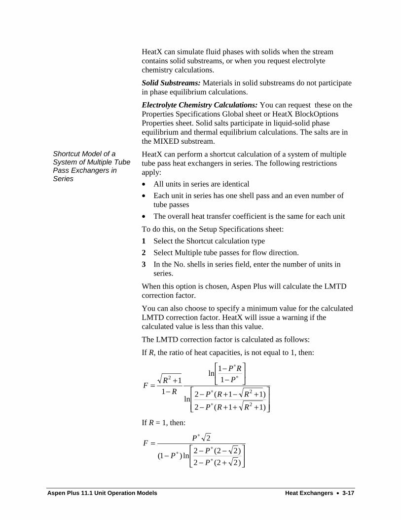
Aspen Plus 11.1 Unit Operation Models Heat Exchangers • 3-17
HeatX can simulate fluid phases with solids when the streamcontains solid substreams, or when you request electrolytechemistry calculations.
Solid Substreams: Materials in solid substreams do not participatein phase equilibrium calculations.
Electrolyte Chemistry Calculations: You can request these on theProperties Specifications Global sheet or HeatX BlockOptionsProperties sheet. Solid salts participate in liquid-solid phaseequilibrium and thermal equilibrium calculations. The salts are inthe MIXED substream.
HeatX can perform a shortcut calculation of a system of multipletube pass heat exchangers in series. The following restrictionsapply:
• All units in series are identical
• Each unit in series has one shell pass and an even number oftube passes
• The overall heat transfer coefficient is the same for each unit
To do this, on the Setup Specifications sheet:
1 Select the Shortcut calculation type
2 Select Multiple tube passes for flow direction.
3 In the No. shells in series field, enter the number of units inseries.
When this option is chosen, Aspen Plus will calculate the LMTDcorrection factor.
You can also choose to specify a minimum value for the calculatedLMTD correction factor. HeatX will issue a warning if thecalculated value is less than this value.
The LMTD correction factor is calculated as follows:
If R, the ratio of heat capacities, is not equal to 1, then:
+++−
+−+−
−−
−+=
∗
∗
∗
∗
)11(2
)11(2ln
1
1ln
1
1
2
2
2
RRP
RRP
P
RP
R
RF
If R = 1, then:
+−−−−
=
∗
∗∗
∗
)22(2
)22(2ln)1(
2
P
PP
PF
Shortcut Model of aSystem of Multiple TubePass Exchangers inSeries
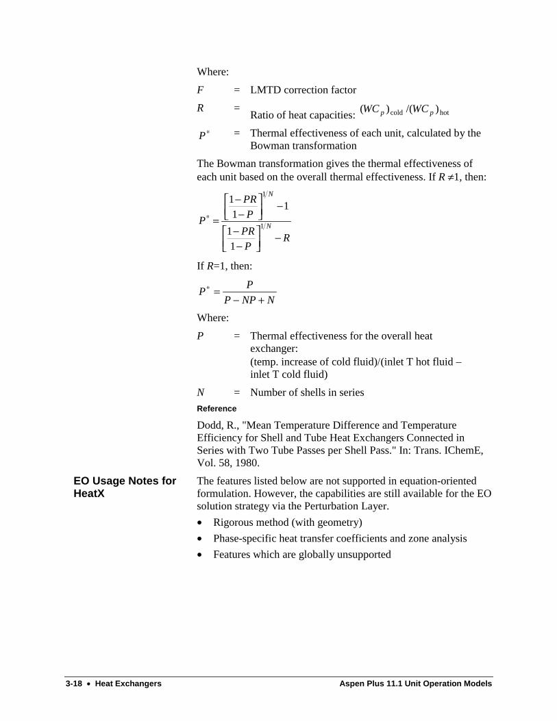
3-18 • Heat Exchangers Aspen Plus 11.1 Unit Operation Models
Where:
F = LMTD correction factor
R =Ratio of heat capacities: hotcold )/()( pp WCWC
∗P = Thermal effectiveness of each unit, calculated by theBowman transformation
The Bowman transformation gives the thermal effectiveness ofeach unit based on the overall thermal effectiveness. If R ≠1, then:
RP
PR
P
PR
PN
N
−
−−
−
−−
=∗1
1
11
11
1
If R=1, then:
NNPP
PP
+−=∗
Where:
P = Thermal effectiveness for the overall heatexchanger:(temp. increase of cold fluid)/(inlet T hot fluid –inlet T cold fluid)
N = Number of shells in series
Reference
Dodd, R., "Mean Temperature Difference and TemperatureEfficiency for Shell and Tube Heat Exchangers Connected inSeries with Two Tube Passes per Shell Pass." In: Trans. IChemE,Vol. 58, 1980.
The features listed below are not supported in equation-orientedformulation. However, the capabilities are still available for the EOsolution strategy via the Perturbation Layer.
• Rigorous method (with geometry)
• Phase-specific heat transfer coefficients and zone analysis
• Features which are globally unsupported
EO Usage Notes forHeatX
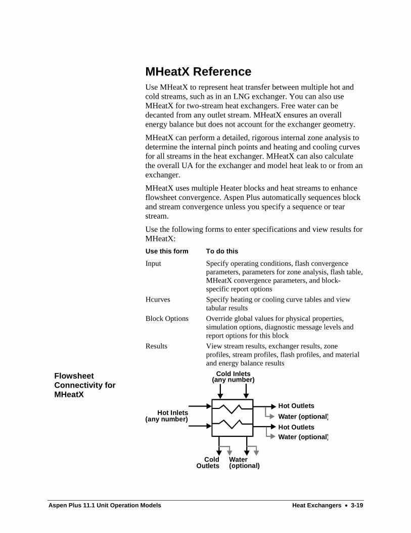
Aspen Plus 11.1 Unit Operation Models Heat Exchangers • 3-19
MHeatX ReferenceUse MHeatX to represent heat transfer between multiple hot andcold streams, such as in an LNG exchanger. You can also useMHeatX for two-stream heat exchangers. Free water can bedecanted from any outlet stream. MHeatX ensures an overallenergy balance but does not account for the exchanger geometry.
MHeatX can perform a detailed, rigorous internal zone analysis todetermine the internal pinch points and heating and cooling curvesfor all streams in the heat exchanger. MHeatX can also calculatethe overall UA for the exchanger and model heat leak to or from anexchanger.
MHeatX uses multiple Heater blocks and heat streams to enhanceflowsheet convergence. Aspen Plus automatically sequences blockand stream convergence unless you specify a sequence or tearstream.
Use the following forms to enter specifications and view results forMHeatX:
Use this form To do this
Input Specify operating conditions, flash convergenceparameters, parameters for zone analysis, flash table,MHeatX convergence parameters, and block-specific report options
Hcurves Specify heating or cooling curve tables and viewtabular results
Block Options Override global values for physical properties,simulation options, diagnostic message levels andreport options for this block
Results View stream results, exchanger results, zoneprofiles, stream profiles, flash profiles, and materialand energy balance results
Hot Inlets(any number)
Hot OutletsWater (optional)
Hot OutletsWater (optional)
Water(optional)
ColdOutlets
Cold Inlets(any number)Flowsheet
Connectivity forMHeatX

3-20 • Heat Exchangers Aspen Plus 11.1 Unit Operation Models
Material Streams
inlet At least one material stream on the hot side, unless a loadstream is used.At least one material stream on the cold side, unless a loadstream is used.
outlet One outlet stream for each inlet stream.One water decant stream for each outlet stream (optional).
Load Streams
inlet Any number of load streams on either or both sides.
outlet One outlet load stream for each inlet load stream.
The inlet stream sides are non-contacting.
You must give outlet specifications for each stream on one side ofthe heat exchanger. On the other side you can specify any of theoutlet streams, but you must leave at least one unspecified stream.
Different streams can have different types of specifications.MHeatX assumes that all unspecified streams have the same outlettemperature. An overall energy balance determines the temperatureof any unspecified stream(s).
You can use a different property method for each stream inMHeatX. Specify the property methods on the BlockOptionsProperties sheet.
MHeatX can perform a detailed, rigorous internal zone analysis todetermine:
• Internal pinch points
• UA and LMTD of each zone
• Total UA of the exchanger
• Overall average LMTD
To obtain a zone analysis, specify Number of zones greater than 0on the MHeatX Input Zone Analysis sheet. During zone analysisMHeatX can add:
• Stream entry points (if all feed streams are not at the sametemperature)
• Stream exit points (if all product streams are not at the sametemperature)
• Phase change points (if a phase change occurs internally)
MHeatX can also account for the nonlinearities of zone profiles byadding zones adaptively. MHeatX can perform zone analysis forboth countercurrent and co-current heat exchangers.
Specifying MHeatX
Zone Analysis
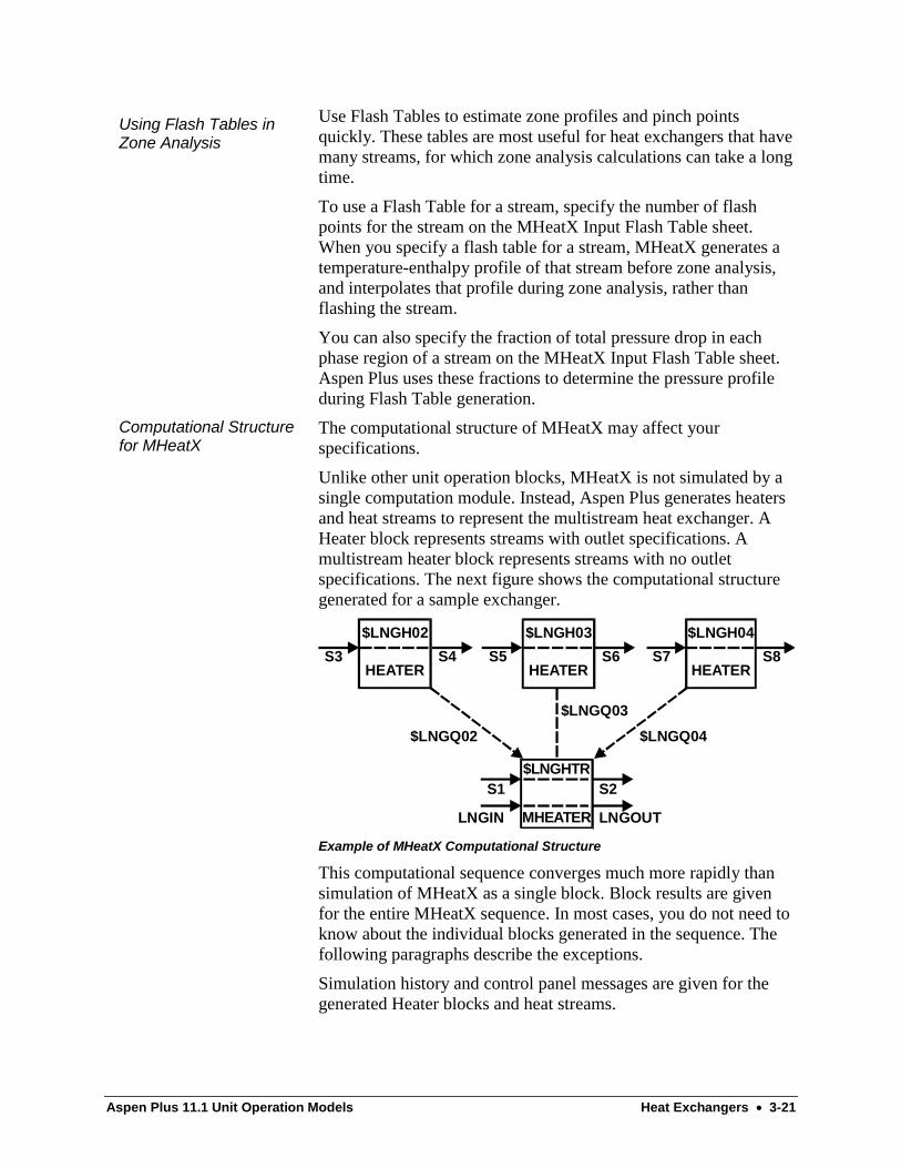
Aspen Plus 11.1 Unit Operation Models Heat Exchangers • 3-21
Use Flash Tables to estimate zone profiles and pinch pointsquickly. These tables are most useful for heat exchangers that havemany streams, for which zone analysis calculations can take a longtime.
To use a Flash Table for a stream, specify the number of flashpoints for the stream on the MHeatX Input Flash Table sheet.When you specify a flash table for a stream, MHeatX generates atemperature-enthalpy profile of that stream before zone analysis,and interpolates that profile during zone analysis, rather thanflashing the stream.
You can also specify the fraction of total pressure drop in eachphase region of a stream on the MHeatX Input Flash Table sheet.Aspen Plus uses these fractions to determine the pressure profileduring Flash Table generation.
The computational structure of MHeatX may affect yourspecifications.
Unlike other unit operation blocks, MHeatX is not simulated by asingle computation module. Instead, Aspen Plus generates heatersand heat streams to represent the multistream heat exchanger. AHeater block represents streams with outlet specifications. Amultistream heater block represents streams with no outletspecifications. The next figure shows the computational structuregenerated for a sample exchanger.
S3 S4 S5 S6 S7 S8
S1 S2
LNGIN LNGOUT
$LNGH03
$LNGQ03
$LNGQ02
HEATER HEATER
$LNGH02
$LNGQ04
HEATER
$LNGH04
$LNGHTR
MHEATER
Example of MHeatX Computational Structure
This computational sequence converges much more rapidly thansimulation of MHeatX as a single block. Block results are givenfor the entire MHeatX sequence. In most cases, you do not need toknow about the individual blocks generated in the sequence. Thefollowing paragraphs describe the exceptions.
Simulation history and control panel messages are given for thegenerated Heater blocks and heat streams.
Using Flash Tables inZone Analysis
Computational Structurefor MHeatX

3-22 • Heat Exchangers Aspen Plus 11.1 Unit Operation Models
You can provide an estimate for duty of the internally generatedheat stream. If the heat stream is a tear stream in the flowsheet,Aspen Plus uses this estimate as an initial value.
You can give convergence specifications for the flowsheetresulting when MHeatX blocks are replaced by their generatednetworks. The generated Heater block and heat stream IDs must beused on the Convergence SequenceSpecifications andConvergence TearSpecifications sheets.
Automatic flowsheet analysis is based on the flowsheet resultingwhen MHeatX blocks are replaced by generated Heater blocks.The generated Heater blocks, instead of the MHeatX block, appearin the calculation sequence. You can select generated heat streamsas tear streams.
MHeatX can simulate fluid phases with solids when the streamcontains solid substreams, or when you request electrolytechemistry calculations.
All phases are in thermal equilibrium. Solids leave at the sametemperature as the fluid phases.
Solid Substreams: Materials in solid substreams do not participatein phase equilibrium calculations.
Electrolyte Chemistry Calculations: You can request these on theProperties Specifications Global sheet or the MHeatXBlockOptions Properties sheet. Solid salts participate in liquid-solid phase equilibrium and thermal equilibrium calculations. Thesalts are in the MIXED substream.
Solids

Aspen Plus 11.1 Unit Operation Models Heat Exchangers • 3-23
Hetran ReferenceHetran is the interface to the B-JAC Hetran program for designingand simulating shell and tube heat exchangers. Hetran can be usedto simulate shell and tube heat exchangers with a wide variety ofconfigurations. To use Hetran, place the block in the flowsheet,connect inlet and outlet streams, and specify a small number ofblock inputs, including the name of the B-JAC input file for thatexchanger.
You enter information related to the heat exchanger configurationand geometry through the Hetran standalone program interface.The exchanger specification is saved as a B-JAC input file. You donot have to enter information about the exchanger’s physicalcharacteristics through the Aspen Plus user interface or throughinput language.
Use the following forms to enter specifications and view results forHetran:
Use this form To do this
Input Specify the name of the B-JAC input file,parameters for calculating the property curves,optional Hetran program inputs, flashconvergence parameters, and valid phases
Block Options Override global values for physical properties,simulation options, diagnostic message levels,and report options for this block
Results View inlet and outlet stream conditions andmaterial and energy balance results
Detailed Results View overall results and detailed results for theshell side and tube side
Cold InletHot Inlet
Hot Water (optional)
Hot OutletCold Outlet
Cold Water (optional)
Material Streams
inlet One hot inletOne cold inlet
FlowsheetConnectivity forHetran

3-24 • Heat Exchangers Aspen Plus 11.1 Unit Operation Models
outlet One hot outletOne cold outletOne water decant stream on the hot side (optional)One water decant stream on the cold side (optional)
Enter the input for the shell and tube heat exchanger through theHetran program’s graphical user interface. The input for Hetran inAspen Plus is limited to:
• The B-JAC input file name that contains the heat exchangerspecification
• A set of parameters to control how property curves aregenerated
• A set of Hetran program inputs that you can change fromwithinAspen Plus (for example, fouling factors and film coefficients)
Use the Flash Options sheet to enter flash specifications.
If you want to perform thesecalculations
Solids? Set Valid Phases to
Vapor phase Yes or no Vapor-only
Liquid phase Yes or no Liquid-only
2-fluid flash phase Yes or no Vapor-Liquid
3-fluid flash phase Yes or no Vapor-Liquid-Liquid
3-fluid phase free-water flash Yes or no Vapor-Liquid-FreeWater
Solids only Yes Solid-only
To override global or flowsheet section property specifications, usethe Flash Options sheet. You can use different physical propertymethods for the hot side and cold side of the heat exchanger. If yousupply only one set of property specifications, Hetran uses that setfor both hot- and cold-side calculations.
Hetran cannot currently handle streams with solids substreams.
Specifying Hetran
Flash Specifications
Physical Properties
Solids

Aspen Plus 11.1 Unit Operation Models Heat Exchangers • 3-25
Aerotran ReferenceAerotran is the interface to the B-JAC Aerotran program fordesigning and simulating air-cooled heat exchangers. Aerotran canbe used to simulate air-cooled heat exchangers with a wide varietyof configurations. It can also be used to model economizers and theconvection section of fired heaters. To use Aerotran, place theblock in the flowsheet, connect inlet and outlet streams, andspecify a small number of block inputs, including the name of theB-JAC input file for that exchanger.
You enter information related to the air cooler configuration andgeometry through the Aerotran standalone program interface. Theair cooler specification is saved as a B-JAC input file. You do nothave to enter information about the air cooler’s physicalcharacteristics through the Aspen Plus user interface or throughinput language.
Use the following forms to enter specifications and view results forAerotran:
Use this form To do this
Input Specify the name of the B-JAC input file,parameters for calculating the property curves,optional Aerotran program inputs, flashconvergence parameters, and valid phases
Block Options Override global values for physical properties,simulation options, diagnostic message levels,and report options for this block
Results View inlet and outlet stream conditions andmaterial and energy balance results
Detailed Results View overall results, detailed results for theoutside and tube side, and fan results
Cold (Air) Inlet
Cold (Air) Outlet
Hot Outlet
Hot Inlet
Hot Water (optional)
Cold Water (optional)FlowsheetConnectivity forAerotran
3-26 • Heat Exchangers Aspen Plus 11.1 Unit Operation Models
Material Streams
inlet One hot inletOne cold (air) inlet
outlet One hot outletOne cold (air) outletOne water decant stream on the hot side (optional)One water decant stream on the cold side (optional)
Enter the input for the air-cooled heat exchanger through theAerotran program’s graphical user interface. The input for Aerotranin Aspen Plus is limited to:
• The B-JAC input file name that contains the heat exchangerspecification
• A set of parameters to control how property curves aregenerated
• A set of Aerotran program inputs that you can change fromwithin Aspen Plus (for example, fouling factors and filmcoefficients)
Use the FlashOptions sheet to enter flash specifications.
If you want to perform thesecalculations
Solids? Set Valid Phases to
Vapor phase Yes or no Vapor-only
Liquid phase Yes or no Liquid-only
2-fluid flash phase Yes or no Vapor-Liquid
3-fluid flash phase Yes or no Vapor-Liquid-Liquid
3-fluid phase free-water flash Yes or no Vapor-Liquid-FreeWater
Solids only Yes Solid-only
To override global or flowsheet section property specifications, usethe FlashOptions sheet. You can use different physical propertymethods for the hot side and cold side of the air cooler. If yousupply only one set of property specifications, Aerotran uses thatset for both hot- and cold-side calculations.
Aerotran blocks cannot currently handle streams with solidssubstreams.
Specifying Aerotran
Flash Specifications
Physical Properties
Solids

Aspen Plus 11.1 Unit Operation Models Heat Exchangers • 3-27
HxFlux ReferenceHxFlux is used to perform heat transfer calculations between a heatsink and a heat source, using convective heat transfer. The drivingforce for the convective heat transfer is calculated as a function oflog-mean temperature difference (LMTD).
Specify variables among inlet and outlet stream temperatures, duty,heat transfer coefficient, and heat transfer area. HxFlux calculatesthe unknown variable and determines the log-mean temperaturedifference, using either the rigorous or the approximate method.
Use the following forms to enter specifications and view results forHxFlux:
Use this form To do this
Input Specify required and optional variables for heat transfercalculations
Results View a summary of results and mass and energybalances.
Heat (optional)
Heat(optional)
inlet Inlet heat stream (optional)
outlet Outlet heat stream (optional)
You have to specify inlet hot stream temperature or temperaturefrom a reference stream, and inlet cold stream temperature ortemperature from a reference stream. You also have to specify fourof the following variables:
• Outlet hot stream (temperature or temperature from a referencestream)
• Outlet cold stream (temperature or temperature from areference stream)
• Duty, duty from a reference heat stream, or inlet heat stream
• Overall heat transfer coefficient
• Heat transfer area
You can select the flow direction for either counter-current or co-current flow. When there is an inlet heat stream or when the duty is
FlowsheetConnectivity forHxFlux
Specifying HxFlux
3-28 • Heat Exchangers Aspen Plus 11.1 Unit Operation Models
from a reference heat stream, you can select the heat streamdirection to indicate whether the duty value is positive or negative.
You can also select the calculation method in determining the log-mean temperature difference.
The standard equation for convective heat transfer is:
LMTDUAQ ⋅=
Where:
Q = Heat duty
U = Overall heat transfer coefficient
A = Heat transfer area
LMTD = Log-mean temperature difference
This equation applies for heat transfer with either counter-currentor co-current flow.
Two methods are used in determining log-mean temperaturedifference (LMTD). For the rigorous method:
∆∆∆−∆
=
2
1
21
lnT
T
TTLMTD
For the approximate method:
321
31
31
2
∆+∆= TT
LMTD
where 1T∆ and 2T∆ are the approach temperatures.
The approximate method is used even if the rigorous method isspecified when:
• Either of the approach temperatures is zero.
• There is no difference in the approach temperatures.
All features of HXFlux are available in the EO formulation, exceptthe features which are globally unsupported.
Convective HeatTransfer
Log-MeanTemperatureDifference
EO Usage Notes forHXFlux
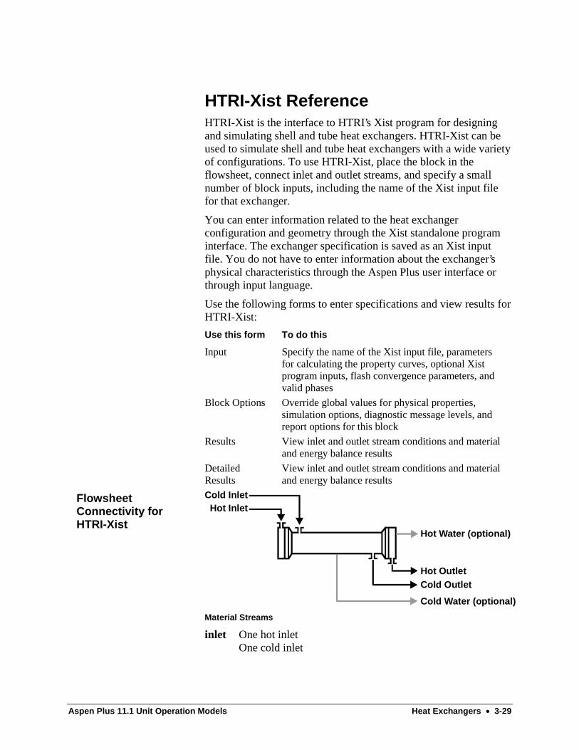
Aspen Plus 11.1 Unit Operation Models Heat Exchangers • 3-29
HTRI-Xist ReferenceHTRI-Xist is the interface to HTRI’s Xist program for designingand simulating shell and tube heat exchangers. HTRI-Xist can beused to simulate shell and tube heat exchangers with a wide varietyof configurations. To use HTRI-Xist, place the block in theflowsheet, connect inlet and outlet streams, and specify a smallnumber of block inputs, including the name of the Xist input filefor that exchanger.
You can enter information related to the heat exchangerconfiguration and geometry through the Xist standalone programinterface. The exchanger specification is saved as an Xist inputfile. You do not have to enter information about the exchanger’sphysical characteristics through the Aspen Plus user interface orthrough input language.
Use the following forms to enter specifications and view results forHTRI-Xist:
Use this form To do this
Input Specify the name of the Xist input file, parametersfor calculating the property curves, optional Xistprogram inputs, flash convergence parameters, andvalid phases
Block Options Override global values for physical properties,simulation options, diagnostic message levels, andreport options for this block
Results View inlet and outlet stream conditions and materialand energy balance results
DetailedResults
View inlet and outlet stream conditions and materialand energy balance results
Cold InletHot Inlet
Hot Water (optional)
Hot OutletCold Outlet
Cold Water (optional)
Material Streams
inlet One hot inletOne cold inlet
FlowsheetConnectivity forHTRI-Xist
3-30 • Heat Exchangers Aspen Plus 11.1 Unit Operation Models
outlet One hot outletOne cold outletOne water decant stream on the hot side (optional)One water decant stream on the cold side (optional)
Enter the input for the shell and tube heat exchanger through theXist program’s graphical user interface. The input for HTRI-Xist inAspen Plus is limited to:
• The Xist input file name that contains the heat exchangerspecification
• A set of parameters to control how property curves aregenerated
• A set of Xist program inputs that you can change from withinAspen Plus (for example, fouling factors and film coefficients)
Use the FlashOptions sheet to enter flash specifications.
If you want to perform thesecalculations
Solids? Set Valid Phases to
Vapor phase Yes or no Vapor-only
Liquid phase Yes or no Liquid-only
2-fluid flash phase Yes or no Vapor-Liquid
3-fluid flash phase Yes or no Vapor-Liquid-Liquid
3-fluid phase free-water flash Yes or no Vapor-Liquid-FreeWater
Solids only Yes Solid-only
To override global or flowsheet section property specifications, usethe FlashOptions sheet. You can use different physical propertymethods for the hot side and cold side of the heat exchanger. If yousupply only one set of property specifications, HTRI-Xist uses thatset for both hot- and cold-side calculations.
HTRI-Xist cannot currently handle streams with solids substreams.
Specifying HTRI-Xist
Flash Specifications
Physical Properties
Solids

Aspen Plus 11.1 Unit Operation Models Columns • 4-1
C H A P T E R 4
Columns
This chapter describes the unit operation models for distillationcolumns using shortcut and rigorous calculations, and for liquid-liquid extraction. The models are:
Model Description Purpose Use For
DSTWU Shortcutdistillation designusing the Winn-Underwood-Gilliland method
Determines minimumreflux ratio, minimumnumber of stages, andeither actual reflux ratio oractual number of stages
Columns with one feed and two productstreams
Distl Shortcutdistillation ratingusing theEdmister method
Determines separationbased on reflux ratio,number of stages, anddistillate-to-feed ratio
Columns with one feed and two productstreams
SCFrac Shortcutdistillation forcomplexpetroleumfractionationunits
Determines productcomposition and flow,number of stages persection, and heat dutyusing fractionation indices
Complex columns, such as crude units andvacuum towers
RadFrac Rigorousfractionation
Performs rigorous ratingand design calculations forsingle columns
Ordinary distillation, absorbers, strippers,extractive and azeotropic distillation, three-phase distillation, reactive distillation
MultiFrac Rigorousfractionation forcomplex columns
Performs rigorous ratingand design calculations formultiple columns of anycomplexity
Heat integrated columns, air separationcolumns, absorber/stripper combinationsethylene plant primary fractionator quenchtower combinations, petroleum refiningapplications
PetroFrac Petroleumrefiningfractionation
Performs rigorous ratingand design calculations forcomplex columns inpetroleum refiningapplications
Preflash tower, atmospheric crude unit, vacuumunit, catalytic cracker main fractionator,delayed coker main fractionator, vacuum lubefractionator, ethylene plant primary fractionatorand quench tower combinations

4-2 • Columns Aspen Plus 11.1 Unit Operation Models
Model Description Purpose Use For
RateFrac† Rate-baseddistillation
Performs rigorous ratingand design for single andmultiple columns. Basedon nonequilibriumcalculations. Does notrequire efficiencies andHETPs.
Distillation columns, absorbers, strippers,reactive systems, heat integrated units,petroleum applications, such as crude andvacuum units, absorber-stripper combination
BatchFrac† Batch distillation Performs rigorouscalculations for batchdistillation
Batch distillation
Extract Rigorous liquid-liquid extraction
Models countercurrentextraction of a liquidstream using a solvent
Liquid-liquid extractors
† RateFrac and BatchFrac require a separate license and can beused only by customers who have purchased it through a specificlicense agreement with Aspen Technology, Inc.
This chapter is organized into the following sections:
Section Models
Shortcut Distillation DSTWU, Distl, SCFrac
Rigorous Distillation RadFrac, MultiFrac, PetroFrac, RateFrac,BatchFrac
Liquid-Liquid Extraction Extract
Aspen Plus 11.1 Unit Operation Models Columns • 4-3
DSTWU ReferenceDSTWU performs shortcut design calculations for single-feed,two-product distillation columns with a partial or total condenser.
DSTWU assumes constant molal overflow and constant relativevolatilities.
DSTWU uses thismethod/correlation
To estimate
Winn Minimum number of stages
Underwood Minimum reflux ratio
Gilliland Required reflux ratio for a specifiednumber of stages or the required numberof stages for a specified reflux ratio
For the specified recovery of light and heavy key components,DSTWU estimates:
• Minimum reflux ratio
• Minimum number of theoretical stages
DSTWU then estimates one of the following:
• Required reflux ratio for the specified number of theoreticalstages
• Required number of theoretical stages for the specified refluxratio
DSTWU also estimates the optimum feed stage location and thecondenser and reboiler duties. DSTWU can produce tables andplots of reflux ratio versus number of stages.
Use the following forms to enter specifications and view results forDSTWU:
Use this form To do this
Input Specify configuration and calculation options,block-specific report options, flash convergenceparameters, valid phases, and DSTWUconvergence parameters
BlockOptions Override global values for physical properties,simulation options, diagnostic message levels, andreport options for this block
Results View summary results, material and energybalance results, and reflux ratio profile
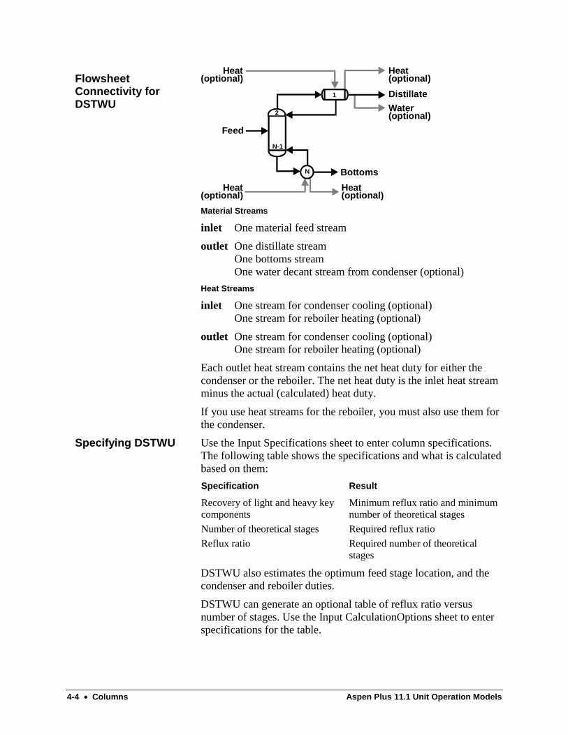
4-4 • Columns Aspen Plus 11.1 Unit Operation Models
Heat(optional)
Heat(optional)
Heat(optional)
Heat(optional)
Water(optional)
Distillate
Feed
Bottoms
1
2
N-1
N
Material Streams
inlet One material feed stream
outlet One distillate streamOne bottoms streamOne water decant stream from condenser (optional)
Heat Streams
inlet One stream for condenser cooling (optional)One stream for reboiler heating (optional)
outlet One stream for condenser cooling (optional)One stream for reboiler heating (optional)
Each outlet heat stream contains the net heat duty for either thecondenser or the reboiler. The net heat duty is the inlet heat streamminus the actual (calculated) heat duty.
If you use heat streams for the reboiler, you must also use them forthe condenser.
Use the Input Specifications sheet to enter column specifications.The following table shows the specifications and what is calculatedbased on them:
Specification Result
Recovery of light and heavy keycomponents
Minimum reflux ratio and minimumnumber of theoretical stages
Number of theoretical stages Required reflux ratio
Reflux ratio Required number of theoreticalstages
DSTWU also estimates the optimum feed stage location, and thecondenser and reboiler duties.
DSTWU can generate an optional table of reflux ratio versusnumber of stages. Use the Input CalculationOptions sheet to enterspecifications for the table.
FlowsheetConnectivity forDSTWU
Specifying DSTWU

Aspen Plus 11.1 Unit Operation Models Columns • 4-5
Distl ReferenceDistl simulates multistage multicomponent columns with a feedstream and two product streams.
Distl performs shortcut distillation rating calculations for a single-feed, two-product distillation column. The column can have eithera partial or total condenser. Distl calculates product compositionusing the Edmister approach. Distl assumes constant moleoverflow and constant relative volatilities.
Use the following forms to enter specifications and view results forDistl:
Use this form To do this
Input Specify basic column configuration, operatingconditions, Distl convergence parameters, and flashconvergence parameters
BlockOptions Override global values for physical properties,simulation options, diagnostic message levels, andreport options for this block
Results View summary of column results and material andenergy balance results
Dynamic Specify parameters for dynamic simulation
Heat(optional)
Heat(optional)
Heat(optional)
Heat(optional)
Water(optional)
Distillate
Feed
Bottoms
1
2
N-1
N
Material Streams
inlet One material feed stream
outlet One distillate streamOne bottoms streamOne water decant stream from condenser (optional)
Heat Streams
inlet One stream for condenser cooling (optional)One stream for reboiler heating (optional)
FlowsheetConnectivity for Distl
4-6 • Columns Aspen Plus 11.1 Unit Operation Models
outlet One stream for condenser cooling (optional)One stream for reboiler heating (optional)
Each outlet heat stream contains the net heat duty for either thecondenser or the reboiler. The net heat duty is the inlet heat streamminus the actual (calculated) heat duty.
If you use heat streams for the reboiler, you must also use them forthe condenser.
Use the Input Specifications sheet to enter the number of stages,reflux ratio, distillate to feed ratio, and other column specifications.
Use the Input Convergence sheet to override default valid phasesfor condenser, convergence parameters for flash calculations, andmodel convergence parameters.
Specifying Distl

Aspen Plus 11.1 Unit Operation Models Columns • 4-7
SCFrac ReferenceUse SCFrac to simulate complex distillation columns with a singlefeed, optional stripping steam, and any number of products.SCFrac also estimates the number of theoretical stages and theheating/cooling duty for each section.
SCFrac can model complex columns, such as crude units andvacuum towers. SCFrac performs shortcut distillation calculationsfor columns with a single feed, one optional stripping steamstream, and any number of products. SCFrac divides a column withn products into n – 1 sections. These sections are numbered fromthe top down. SCFrac assumes:
• Relative volatilities are constant for each section
• The flow of liquid from section to section is negligible
SCFrac does not handle solids. SCFrac can perform free-watercalculations in the condenser.
Use the following forms to enter specifications and view results forSCFrac:
Use this form To do this
Input Specify operating parameters, valid phases, SCFracconvergence parameters, and flash convergenceparameters
Block Options Override global values for physical properties,simulation options, diagnostic message levels, andreport options for this block
Results View condenser results, material and energybalance results, design specification results, sectionprofiles, and product summary
Steam(optional)
Distillate
Bottoms
Side Products(any number)
Feed
Material Streams
inlet One material feed streamOne optional stripping steam stream (used for all sections)
FlowsheetConnectivity forSCFrac
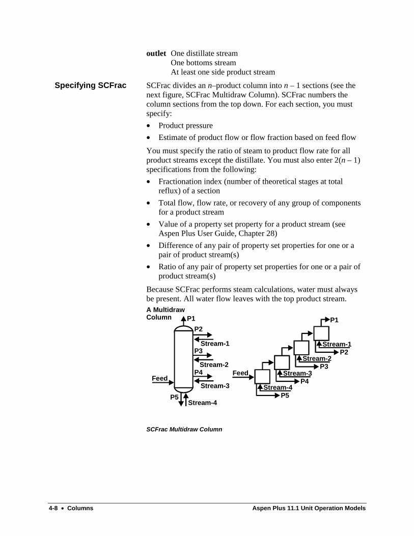
4-8 • Columns Aspen Plus 11.1 Unit Operation Models
outlet One distillate streamOne bottoms streamAt least one side product stream
SCFrac divides an n–product column into n – 1 sections (see thenext figure, SCFrac Multidraw Column). SCFrac numbers thecolumn sections from the top down. For each section, you mustspecify:
• Product pressure
• Estimate of product flow or flow fraction based on feed flow
You must specify the ratio of steam to product flow rate for allproduct streams except the distillate. You must also enter 2(n – 1)specifications from the following:
• Fractionation index (number of theoretical stages at totalreflux) of a section
• Total flow, flow rate, or recovery of any group of componentsfor a product stream
• Value of a property set property for a product stream (seeAspen Plus User Guide, Chapter 28)
• Difference of any pair of property set properties for one or apair of product stream(s)
• Ratio of any pair of property set properties for one or a pair ofproduct stream(s)
Because SCFrac performs steam calculations, water must alwaysbe present. All water flow leaves with the top product stream.A MultidrawColumn P1
P2
P3
P4
P5
Stream-1
P1
P2Stream-1
P3Stream-2
P4
P5
Stream-3
Stream-4
Stream-2
Stream-3
Stream-4
FeedFeed
SCFrac Multidraw Column
Specifying SCFrac

Aspen Plus 11.1 Unit Operation Models Columns • 4-9
RadFrac ReferenceRadFrac is a rigorous model for simulating all types of multistagevapor-liquid fractionation operations. These operations include:
• Ordinary distillation
• Absorption
• Reboiled absorption
• Stripping
• Reboiled stripping
• Extractive and azeotropic distillation
RadFrac is suitable for:
• Two-phase systems
• Three-phase systems
• Narrow and wide-boiling systems
• Systems exhibiting strong liquid phase nonideality
RadFrac can detect and handle a free-water phase or other secondliquid phase anywhere in the column. RadFrac can handle solidson every stage.
RadFrac can handle pumparounds leaving any stage and returningto the same stage or to a different stage.
RadFrac can model columns in which chemical reactions areoccurring. Reactions can have fixed conversions, or they can be:
• Equilibrium
• Rate-controlled
• Electrolytic
RadFrac can also model columns in which two liquid phases andchemical reactions occur simultaneously, using different reactionkinetics for the two liquid phases. In addition, RadFrac can modelsalt precipitation.
Although RadFrac assumes equilibrium stages, you can specifyeither Murphree or vaporization efficiencies. You can manipulateMurphree efficiencies to match plant performance.
You can use RadFrac to size and rate columns consisting of traysand/or packings. RadFrac can model both random and structuredpackings.
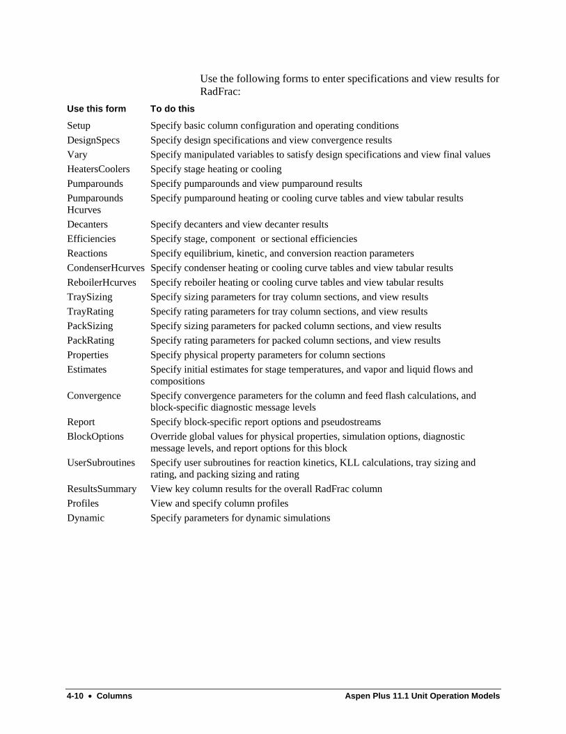
4-10 • Columns Aspen Plus 11.1 Unit Operation Models
Use the following forms to enter specifications and view results forRadFrac:
Use this form To do this
Setup Specify basic column configuration and operating conditions
DesignSpecs Specify design specifications and view convergence results
Vary Specify manipulated variables to satisfy design specifications and view final values
HeatersCoolers Specify stage heating or cooling
Pumparounds Specify pumparounds and view pumparound results
PumparoundsHcurves
Specify pumparound heating or cooling curve tables and view tabular results
Decanters Specify decanters and view decanter results
Efficiencies Specify stage, component or sectional efficiencies
Reactions Specify equilibrium, kinetic, and conversion reaction parameters
CondenserHcurves Specify condenser heating or cooling curve tables and view tabular results
ReboilerHcurves Specify reboiler heating or cooling curve tables and view tabular results
TraySizing Specify sizing parameters for tray column sections, and view results
TrayRating Specify rating parameters for tray column sections, and view results
PackSizing Specify sizing parameters for packed column sections, and view results
PackRating Specify rating parameters for packed column sections, and view results
Properties Specify physical property parameters for column sections
Estimates Specify initial estimates for stage temperatures, and vapor and liquid flows andcompositions
Convergence Specify convergence parameters for the column and feed flash calculations, andblock-specific diagnostic message levels
Report Specify block-specific report options and pseudostreams
BlockOptions Override global values for physical properties, simulation options, diagnosticmessage levels, and report options for this block
UserSubroutines Specify user subroutines for reaction kinetics, KLL calculations, tray sizing andrating, and packing sizing and rating
ResultsSummary View key column results for the overall RadFrac column
Profiles View and specify column profiles
Dynamic Specify parameters for dynamic simulations

Aspen Plus 11.1 Unit Operation Models Columns • 4-11
RadFrac can have any number of:
• Stages
• Interstage heaters/coolers
• Decanters
• Pumparounds
Material Streams
inlet At least one inlet material stream
outlet One vapor or liquid distillate product stream, or bothOne water distillate product stream (optional)One bottoms liquid product streamUp to three side product streams per stage (optional)Any number of pseudo-product streams (optional)
Each stage can have:
• Any number of inlet streams
• Up to three outlet streams (one vapor and two liquid)
Outlet streams can be partial or total drawoffs of the stage flows.
Decanter outlet streams can return to the stage immediately below.Or they can be split into any number of streams, each returning to adifferent user-specified stage. Pumparounds can go between anytwo stages, or to the same stage.
Any number of pseudoproduct streams can represent columninternal flows, pumparound flows, and thermosyphon reboilerflows. A pseudoproduct stream does not affect column results.
Heat Streams
inlet One inlet heat stream per stage (optional)One heat stream per pumparound (optional)
outlet One outlet heat stream per stage (optional)One heat stream per pumparound (optional)
FlowsheetConnectivity forRadFrac

4-12 • Columns Aspen Plus 11.1 Unit Operation Models
RadFrac uses an inlet heat stream as a duty specification for allstages except the condenser, reboiler, and pumparounds. If you donot give two column operating specifications on the SetupConfiguration sheet, RadFrac uses a heat stream as a specificationfor the condenser and reboiler. If you do not give twospecifications on the Pumparounds Specifications sheet, RadFracuses a heat stream as a specification for pumparounds.
If you give two specifications on the Setup Configuration sheet orPumparounds Specifications sheet, RadFrac does not use the inletheat stream as a specification. The inlet heat stream supplies therequired heating or cooling.
Use optional outlet streams for the net heat duty of the condenser,reboiler, and pumparounds. The value of the outlet heat streamequals the value of the inlet heat stream (if any) minus the actual(calculated) heat duty.
This section describes the following topics on RadFrac columnconfiguration:
• Stage Numbering
• Feed Stream Conventions
• Columns Without Condensers or Reboilers
• Reboiler Handling
• Heater and Cooler Specifications
• Decanters
• Pumparounds
RadFrac numbers stages from the top down, starting with thecondenser (or starting with the top stage if there is no condenser).
Use the Setup Streams sheet to specify the feed and product stages.
RadFrac provides three conventions for handling feed streams:
• Above-Stage
• On-Stage
• Decanter (for three phase calculations only)
(See the following figures, RadFrac Feed Convention Above-Stageand RadFrac Feed Convention On-Stage.)
When the feed convention is Above-Stage, RadFrac introduces amaterial stream between adjacent stages. The liquid portion flowsto the stage you specify. The vapor portion flows to the stageabove. You can introduce a liquid feed to the top stage (orcondenser) by specifying Stage=1. You can introduce a vapor feedto the bottom stage (or reboiler) by specifying Stage= the numberof equilibrium stages + 1. Feed convention Decanter is used only
Specifying RadFrac
Stage Numbering
Feed StreamConventions

Aspen Plus 11.1 Unit Operation Models Columns • 4-13
in three-phase calculations (Valid Phases=Vapor-Liquid-Liquid onthe Setup Configuration sheet) involving decanters. You canintroduce a feed directly to a decanter attached to a stage using thisconvention.
Vapor
Liquid
Mixed feed tostage n
n - 1
n
RadFrac Feed Convention Above-Stage
Mixed feed tostage n
n - 1
n
RadFrac Feed Convention On-Stage
When the Feed Convention is On-Stage, both the liquid and vaporportions of a feed flow to the stage you specify.
You can specify the column configuration on the SetupConfiguration sheet.
If the column has no Then specify On sheet
Condenser None forCondenser
Setup Configuration
Reboiler None forReboiler
Setup Configuration
RadFrac can model two reboiler types:
• Kettle
• Thermosyphon
A kettle reboiler is modeled as the last stage in the column on theSetup Configuration sheet. Select Kettle for reboiler. By default,RadFrac uses a kettle reboiler. To specify the reboiler duty, enter
Columns WithoutCondensers or Reboilers
Reboiler Handling
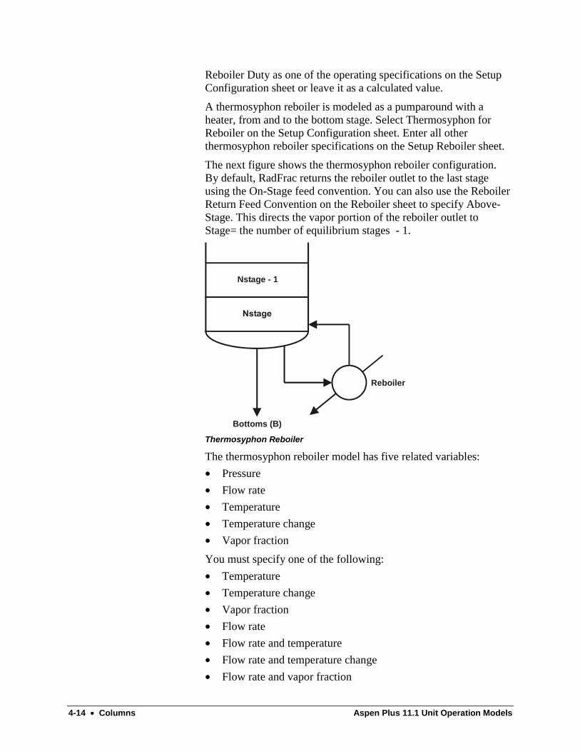
4-14 • Columns Aspen Plus 11.1 Unit Operation Models
Reboiler Duty as one of the operating specifications on the SetupConfiguration sheet or leave it as a calculated value.
A thermosyphon reboiler is modeled as a pumparound with aheater, from and to the bottom stage. Select Thermosyphon forReboiler on the Setup Configuration sheet. Enter all otherthermosyphon reboiler specifications on the Setup Reboiler sheet.
The next figure shows the thermosyphon reboiler configuration.By default, RadFrac returns the reboiler outlet to the last stageusing the On-Stage feed convention. You can also use the ReboilerReturn Feed Convention on the Reboiler sheet to specify Above-Stage. This directs the vapor portion of the reboiler outlet toStage= the number of equilibrium stages - 1.
Reboiler
Nstage - 1
Bottoms (B)
Thermosyphon Reboiler
The thermosyphon reboiler model has five related variables:
• Pressure
• Flow rate
• Temperature
• Temperature change
• Vapor fraction
You must specify one of the following:
• Temperature
• Temperature change
• Vapor fraction
• Flow rate
• Flow rate and temperature
• Flow rate and temperature change
• Flow rate and vapor fraction

Aspen Plus 11.1 Unit Operation Models Columns • 4-15
If you choose an option consisting of two variables, you mustspecify the reboiler heat duty on the Setup Configuration sheet.RadFrac treats the value you enter for the reboiler heat duty as aninitial estimate.
The reboiler pressure is optional. If you do not enter a value,RadFrac uses the bottom stage pressure.
You can specify interstage heaters and coolers in one of two ways:
• Specifying the duty directly on the HeatersCoolers SideDutiessheet
• Requesting UA calculations on the HeatersCoolersUtilityExchangers sheet
If you specify the duty directly on the HeatersCoolers SideDutiessheet, enter a positive duty for heating and a negative duty forcooling.
If you request UA calculations on the HeatersCoolersUtilityExchangers sheet, RadFrac calculates the duty and outlettemperature of the heating/cooling fluid simultaneously with thecolumn. The UA calculations:
• Assume the stage temperature is constant
• Use an arithmetic average temperature difference
• Assume the heating or cooling fluid does not experience anyphase change
To request UA calculations, specify the:
• UA
• Heating or cooling fluid component
• Flow and inlet temperature of the fluid
You can specify the heat capacity of the fluid directly on theHeatersCoolers UtilityExchangers sheet or RadFrac can compute itfrom a property method. If RadFrac computes the heat capacity,you must also enter the pressure and phase of the heating orcooling fluid. By default, RadFrac calculates the heat capacityusing the block property method. But you can also use a differentproperty method.
You can also specify the heat loss for sections of the column on theHeatersCoolers HeatLoss sheet.
For three-phase calculations (Valid Phases=Vapor-Liquid-Liquidon the Setup Configuration sheet), you can define any number ofdecanters. Enter decanter specifications on the Decanters form.
For the decanter on the top stage, you must enter the return fractionof at least one of the two liquid phases (Fraction of 1st Liquid
Heater and CoolerSpecifications
Decanters

4-16 • Columns Aspen Plus 11.1 Unit Operation Models
Returned, Fraction of 2nd Liquid Returned on the DecantersSpecifications sheet). For decanters on other stages, you mustalways specify both Fraction of 1st Liquid Returned and Fractionof 2nd Liquid Returned.
You can enter Temperature and Degrees Subcooling on theDecanters Options sheet to model subcooled decanters. If you donot specify Temperature and Degrees Subcooling, the decanter isoperated at the temperature of the stage to which the decanter isattached. If side product streams are decanter products, you cannotspecify their flow rates. RadFrac calculates their flow rates fromthe Fraction of 1st Liquid Returned and Fraction of 2nd LiquidReturned.
By default RadFrac returns decanter streams to the stageimmediately below. You can return the decanter streams to anyother stage by entering a different Return Stage number on theDecanters Specifications sheet. You can split a return stream intoany number of streams by giving a split fraction (Split Fraction ofTotal Return for the 1st Liquid and 2nd Liquid). Each resultingstream may go to a different return stage.
When return streams do not go to the next stage, a feed orpumparound must go to the next stage. This prevents dry stages.
RadFrac can handle pumparounds from any stage to the same orany other stage. Use the Pumparounds form to enter allpumparound specifications.
You must enter the source and destination stage locations forpumparounds. A pumparound can be either a partial or totaldrawoff of the:
• Stage liquid
• First liquid phase
• Second liquid phase
• Vapor phase
You can associate a heater or cooler with a pumparound. If thepumparound is a partial drawoff of the stage flow, you must entertwo of the following specifications:
• Flow rate
• Temperature
• Temperature change
• Vapor fraction
• Heat Duty
Pumparounds

Aspen Plus 11.1 Unit Operation Models Columns • 4-17
If the pumparound is a total drawoff, you must enter one of thefollowing specifications:
• Temperature
• Temperature change
• Vapor fraction
• Heat Duty
Vapor fraction is allowed only when Valid Phases=Vapor-Liquidor Vapor-Liquid-Liquid.
Use the Pumparounds Specifications sheet to enter these operatingspecifications.
Pressure specification is optional. The default pumparoundpressure is the same as the source stage pressure. RadFrac assumesthat the pumparound at the heater/cooler outlet has the same phasecondition as the pumparound at the inlet. You can override thephase condition using the Valid phases field on PumparoundSpecifications sheet.
RadFrac can return the pumparound to a stage using either the:
• On-stage option
• Above-stage option (returns the pumparound to the columnbetween two stages)
In three-phase columns, RadFrac can also return the pumparoundto a decanter associated with a stage. You can select above-stageusing the Return option field.
RadFrac assumes the pumparound at the heater/cooler outlet hasthe same phase condition as the inlet.
You can use Return-Phase on the Pumparounds Specificationssheet to assign a different phase at the heater/cooler outlet. Or youcan specify Valid Phases=VaporLiquid or Vapor-Liquid-Liquidand let RadFrac determine the return phase condition from theheater/cooler specifications.
The features listed below are not supported in equation-orientedformulation. However, the capabilities are still available for the EOsolution strategy via the Perturbation Layer.
• Thermosyphon Reboiler *
• TPSAR with pressure update
• Features which are globally unsupported
* Thermosyphon reboiler is supported in the EO formulation whenvfrac is one of the specifications.
EO Usage Notes forRadFrac

4-18 • Columns Aspen Plus 11.1 Unit Operation Models
RadFrac is capable of performing three-phase calculations in theequation-oriented formulation. By default, the EO formulationassumes the same stages will have three-phase separation as in thesequential-modular solution. You can force the EO formulation tocheck for three-phase separation on all stages specified on theRadFrac | Setup | 3-Phase sheet by selecting the checkbox for thePhase splitting on all specified trays option on the RadFrac |Block Options | EO Options | Additional Variables dialog box..
When three-phase calculations are specified, RadFrac checks thefinal EO solution for missed three-phase separation (on stagesmodeled as two-phase) using Gibbs free energy minimization. Ifsuch three-phase separation is found, RadFrac issues an error. Youcan either reconcile results with SM and run again, or use thePhase splitting on all specified trays option to specify the stageswhere RadFrac should look for three-phase separation.
RadFrac can perform both free-water and rigorous three-phasecalculations. (See Aspen Plus Physical Property Methods andModels, Chapter 6.) These calculations are controlled by optionsyou specify on the Setup Configuration sheet.
You can select from three types of calculations:
• Free water in the condenser only
• Free water on any or all stages
• Rigorous three-phase calculations
When you choose free-water calculations in the condenser, onlyfree water can be decanted from the condenser. You cannot usenonideal for the Overall Loop convergence method.
Specify one of the following on the Setup Configuration sheet:
Valid Phases= On Sheet For
Vapor-Liquid-FreeWaterCondenser
SetupConfiguration
Free water in thecondenser only
Vapor-Liquid-FreeWaterAnyStage
SetupConfiguration
Free water on allstages
Vapor-Liquid-Liquid SetupConfiguration
Rigorous three-phasecalculations
For RadFrac calculations, you must also specify which stages totest for two liquid phases on the Setup 3-Phase sheet.
When you choose completely rigorous three-phase calculations onall stages selected, RadFrac makes no assumptions about the natureof the two liquid phases. You can associate a decanter with anystage. You cannot use Sum-Rates for the Overall Loopconvergence method.
Free-Water andRigorous Three-Phase Calculations
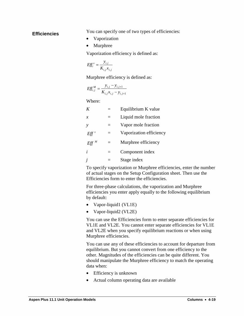
Aspen Plus 11.1 Unit Operation Models Columns • 4-19
You can specify one of two types of efficiencies:
• Vaporization
• Murphree
Vaporization efficiency is defined as:
Effy
K xiv i j
i j i j
= ,
, ,
Murphree efficiency is defined as:
Effy y
K x yi jM i j i j
i j i j i j,
, ,
, , ,
=−−
+
+
1
1
Where:
K = Equilibrium K value
x = Liquid mole fraction
y = Vapor mole fraction
Eff v = Vaporization efficiency
Eff M = Murphree efficiency
i = Component index
j = Stage index
To specify vaporization or Murphree efficiencies, enter the numberof actual stages on the Setup Configuration sheet. Then use theEfficiencies form to enter the efficiencies.
For three-phase calculations, the vaporization and Murphreeefficiencies you enter apply equally to the following equilibriumby default:
• Vapor-liquid1 (VL1E)
• Vapor-liquid2 (VL2E)
You can use the Efficiencies form to enter separate efficiencies forVL1E and VL2E. You cannot enter separate efficiencies for VL1Eand VL2E when you specify equilibrium reactions or when usingMurphree efficiencies.
You can use any of these efficiencies to account for departure fromequilibrium. But you cannot convert from one efficiency to theother. Magnitudes of the efficiencies can be quite different. Youshould manipulate the Murphree efficiency to match the operatingdata when:
• Efficiency is unknown
• Actual column operating data are available
Efficiencies
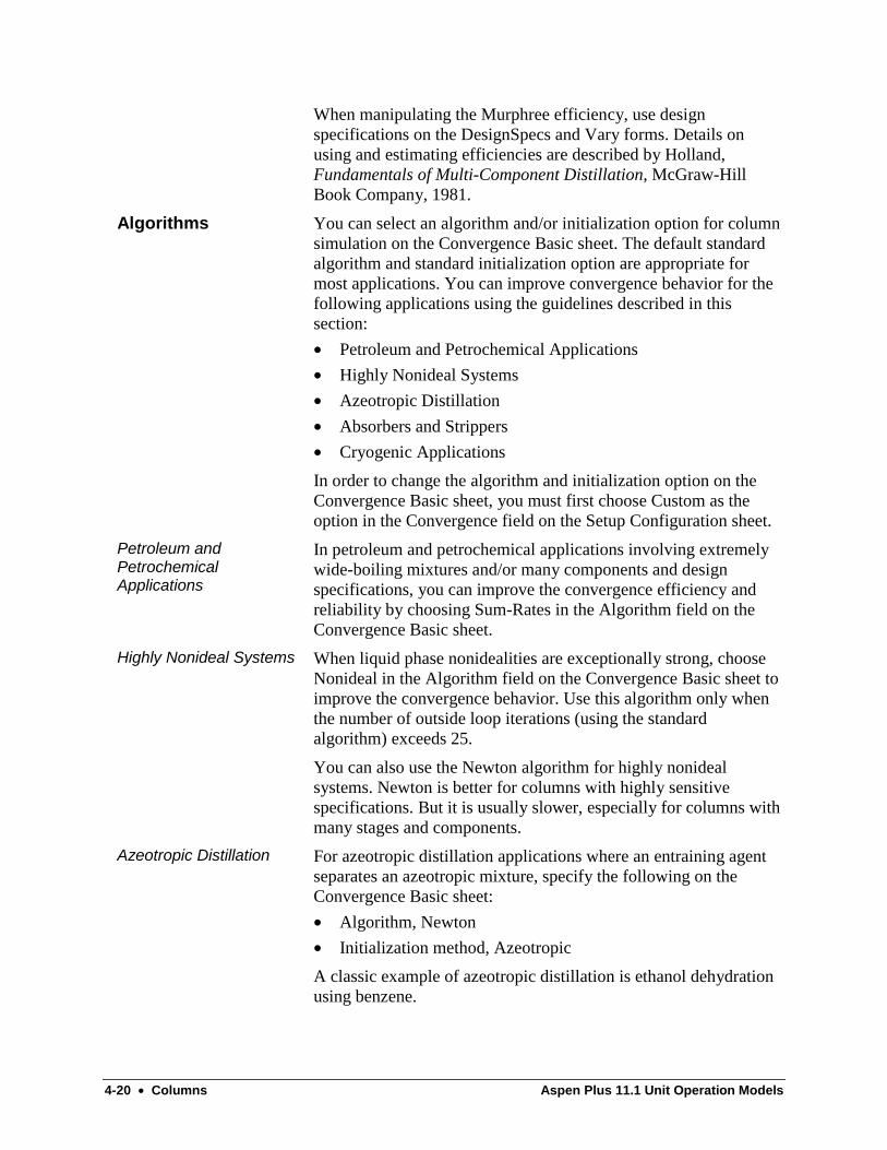
4-20 • Columns Aspen Plus 11.1 Unit Operation Models
When manipulating the Murphree efficiency, use designspecifications on the DesignSpecs and Vary forms. Details onusing and estimating efficiencies are described by Holland,Fundamentals of Multi-Component Distillation, McGraw-HillBook Company, 1981.
You can select an algorithm and/or initialization option for columnsimulation on the Convergence Basic sheet. The default standardalgorithm and standard initialization option are appropriate formost applications. You can improve convergence behavior for thefollowing applications using the guidelines described in thissection:
• Petroleum and Petrochemical Applications
• Highly Nonideal Systems
• Azeotropic Distillation
• Absorbers and Strippers
• Cryogenic Applications
In order to change the algorithm and initialization option on theConvergence Basic sheet, you must first choose Custom as theoption in the Convergence field on the Setup Configuration sheet.
In petroleum and petrochemical applications involving extremelywide-boiling mixtures and/or many components and designspecifications, you can improve the convergence efficiency andreliability by choosing Sum-Rates in the Algorithm field on theConvergence Basic sheet.
When liquid phase nonidealities are exceptionally strong, chooseNonideal in the Algorithm field on the Convergence Basic sheet toimprove the convergence behavior. Use this algorithm only whenthe number of outside loop iterations (using the standardalgorithm) exceeds 25.
You can also use the Newton algorithm for highly nonidealsystems. Newton is better for columns with highly sensitivespecifications. But it is usually slower, especially for columns withmany stages and components.
For azeotropic distillation applications where an entraining agentseparates an azeotropic mixture, specify the following on theConvergence Basic sheet:
• Algorithm, Newton
• Initialization method, Azeotropic
A classic example of azeotropic distillation is ethanol dehydrationusing benzene.
Algorithms
Petroleum andPetrochemicalApplications
Highly Nonideal Systems
Azeotropic Distillation

Aspen Plus 11.1 Unit Operation Models Columns • 4-21
To model absorbers and strippers specify Condenser=None andReboiler=None on the Setup Configuration sheet. The heat duty iszero for adiabatic operation. For extremely wide-boiling mixtures,specify one of the following:
• Algorithm=Sum-Rates on the Convergence Basic sheet
• Convergence=Standard on the Setup Configuration sheet andchoose Absorber=Yes on the Convergence Basic sheet
For cryogenic applications such as air separation, the standardalgorithm is recommended. To invoke a special initializationprocedure designed for cryogenic systems, specify Cryogenic forInitialization on the Convergence Basic sheet.
RadFrac allows the column to be operated in a rating mode or adesign mode. Rating mode requires different column specificationsfor two- and three-phase calculations.
For two-phase calculations, you must enter the following on theSetup Form:
• Valid Phases=Vapor-Liquid or Vapor-Liquid-FreeWaterCondenser for handling free water in condenser
• A Total, Subcooled, or Partial-Vapor condenser
• Two additional column operating variables
If the condenser or reflux is subcooled, you can also specify thedegrees subcooling or the subcooled temperature.
For three-phase calculations, you must specify Valid Phases=Vapor-Liquid-Liquid or Vapor-Liquid-FreeWaterAnyStage (forfree water calculations) on the Setup Configuration sheet. Therequired specifications depend on what you specify for the returnfractions of the two liquid phases (Fraction of 1st Liquid Returnedand Fraction of 2nd Liquid Returned) in the top stage decanter.The following table lists the three specification options:
If you specified this onDecanters Specifications Enter on Setup Configuration
Fraction of 1st Liquid Returnedor Fraction of 2nd LiquidReturned, or no top decanter
A Total, Subcooled, or Partial-Vaporcondenser and two operatingspecifications
Fraction of 1st Liquid Returnedand Fraction of 2nd LiquidReturned
A Total, Subcooled, or Partial-Vaporcondenser and one operatingspecification
Fraction of 1st Liquid Returnedand Fraction of 2nd LiquidReturned
Two operating specifications, and anestimate for the amount of vapor in thedistillate on the Estimates VaporComposition sheet. RadFrac assumes apartial condenser with both vapor andliquid distillates.
Absorbers and Strippers
Cryogenic Applications
Rating Mode
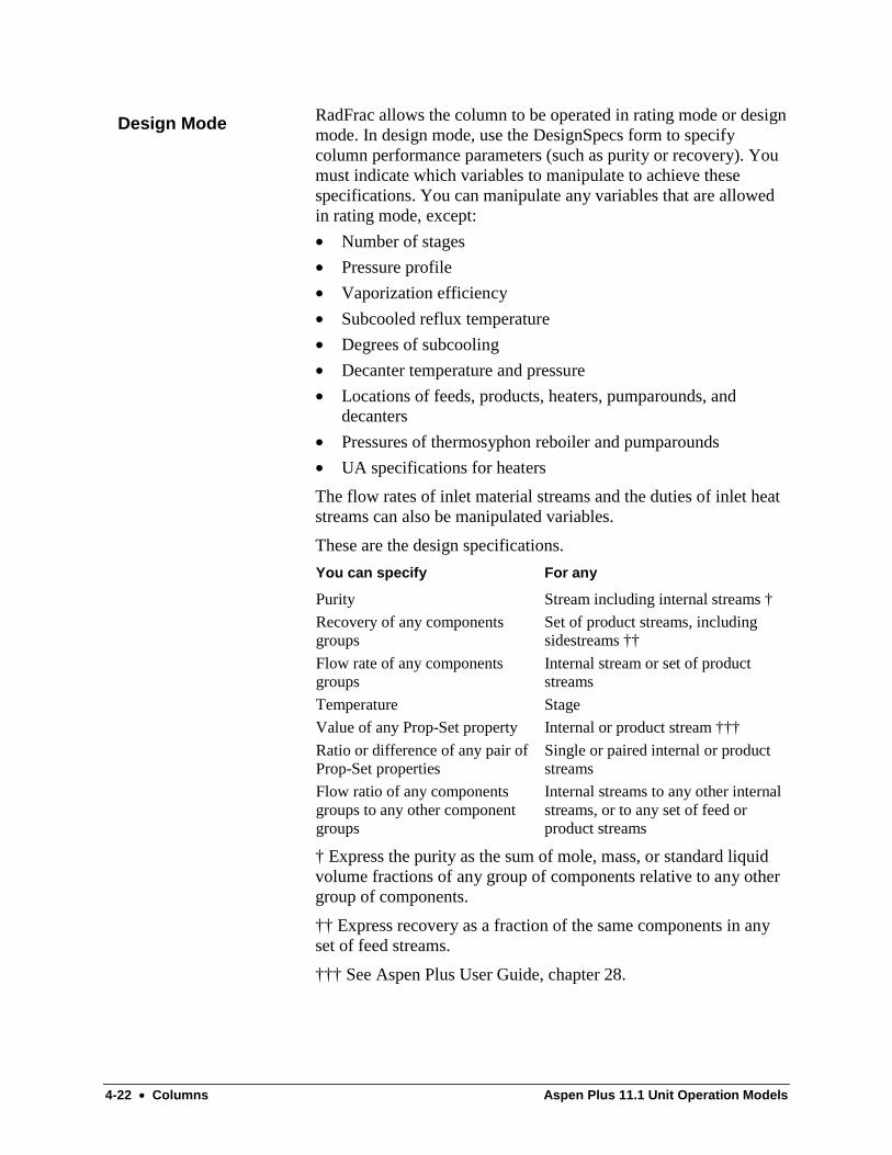
4-22 • Columns Aspen Plus 11.1 Unit Operation Models
RadFrac allows the column to be operated in rating mode or designmode. In design mode, use the DesignSpecs form to specifycolumn performance parameters (such as purity or recovery). Youmust indicate which variables to manipulate to achieve thesespecifications. You can manipulate any variables that are allowedin rating mode, except:
• Number of stages
• Pressure profile
• Vaporization efficiency
• Subcooled reflux temperature
• Degrees of subcooling
• Decanter temperature and pressure
• Locations of feeds, products, heaters, pumparounds, anddecanters
• Pressures of thermosyphon reboiler and pumparounds
• UA specifications for heaters
The flow rates of inlet material streams and the duties of inlet heatstreams can also be manipulated variables.
These are the design specifications.
You can specify For any
Purity Stream including internal streams †
Recovery of any componentsgroups
Set of product streams, includingsidestreams ††
Flow rate of any componentsgroups
Internal stream or set of productstreams
Temperature Stage
Value of any Prop-Set property Internal or product stream †††
Ratio or difference of any pair ofProp-Set properties
Single or paired internal or productstreams
Flow ratio of any componentsgroups to any other componentgroups
Internal streams to any other internalstreams, or to any set of feed orproduct streams
† Express the purity as the sum of mole, mass, or standard liquidvolume fractions of any group of components relative to any othergroup of components.
†† Express recovery as a fraction of the same components in anyset of feed streams.
††† See Aspen Plus User Guide, chapter 28.
Design Mode

Aspen Plus 11.1 Unit Operation Models Columns • 4-23
RadFrac can handle chemical reactions. These reactions can occurin the liquid and/or vapor phase. The details about the reactions areentered on a generic Reactions form outside RadFrac. RadFracallows two different reaction model types: REAC-DIST or USER.RadFrac can model the following types of reactions:
• Equilibrium-controlled
• Rate-controlled
• Conversion
• Electrolytic
RadFrac can also model salt precipitation, especially in the case ofelectrolytic systems. You can request reaction calculations for theentire column, or you can restrict reactions to a certain columnsegment (for example, to model the presence of catalyst). Forthree-phase calculations, you can restrict reactions to one of thetwo liquid phases, or use separate reaction kinetics for the twoliquid phases.
To include reactions in RadFrac you must enter the followinginformation on the Reactions Specifications sheet:
• Reaction type and Reaction/Chemistry ID
• Column section in which the reactions occur
Depending on the reaction type, you must enter equilibriumconstant, kinetic, or conversion parameters on the genericReactions form outside RadFrac. For electrolytic reactions, youcan also enter the reaction data on the Reactions Chemistry formoutside RadFrac. To consider salt precipitation, enter the saltprecipitation parameters on the Reactions Salt sheet or theReactions Chemistry form outside RadFrac.
To associate reactions and salt precipitation with a columnsegment, enter the corresponding Reactions ID (or Chemistry ID)on the Reactions Specifications sheet.
For rate-controlled reactions, you must enter holdup or residencetime data in the phase where the reactions occur. Use the ReactionsHoldups or Residence Times sheets. For conversion reactions, usethe Reactions Conversion sheet to override the conversionparameters specified on the Reactions Conversion form. RadFracalso supports User Reaction Subroutine. The name and otherdetails of the reaction subroutine are entered on theUserSubroutines form.
Reactive Distillation
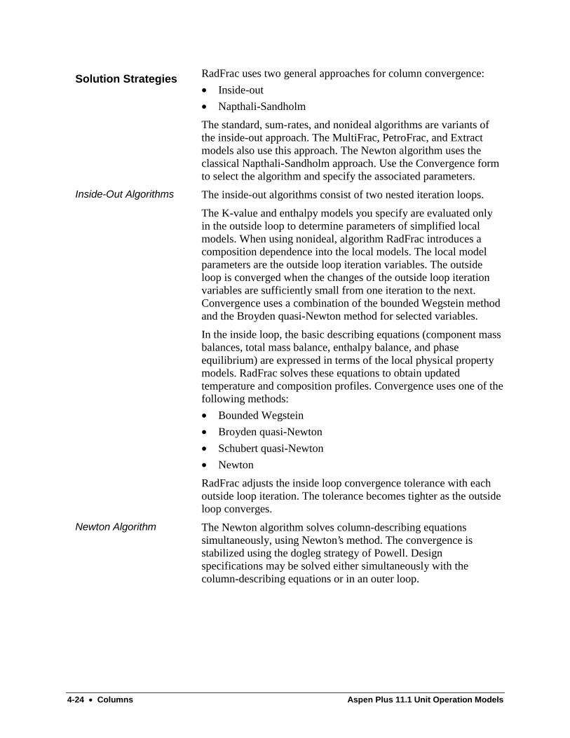
4-24 • Columns Aspen Plus 11.1 Unit Operation Models
RadFrac uses two general approaches for column convergence:
• Inside-out
• Napthali-Sandholm
The standard, sum-rates, and nonideal algorithms are variants ofthe inside-out approach. The MultiFrac, PetroFrac, and Extractmodels also use this approach. The Newton algorithm uses theclassical Napthali-Sandholm approach. Use the Convergence formto select the algorithm and specify the associated parameters.
The inside-out algorithms consist of two nested iteration loops.
The K-value and enthalpy models you specify are evaluated onlyin the outside loop to determine parameters of simplified localmodels. When using nonideal, algorithm RadFrac introduces acomposition dependence into the local models. The local modelparameters are the outside loop iteration variables. The outsideloop is converged when the changes of the outside loop iterationvariables are sufficiently small from one iteration to the next.Convergence uses a combination of the bounded Wegstein methodand the Broyden quasi-Newton method for selected variables.
In the inside loop, the basic describing equations (component massbalances, total mass balance, enthalpy balance, and phaseequilibrium) are expressed in terms of the local physical propertymodels. RadFrac solves these equations to obtain updatedtemperature and composition profiles. Convergence uses one of thefollowing methods:
• Bounded Wegstein
• Broyden quasi-Newton
• Schubert quasi-Newton
• Newton
RadFrac adjusts the inside loop convergence tolerance with eachoutside loop iteration. The tolerance becomes tighter as the outsideloop converges.
The Newton algorithm solves column-describing equationssimultaneously, using Newton’s method. The convergence isstabilized using the dogleg strategy of Powell. Designspecifications may be solved either simultaneously with thecolumn-describing equations or in an outer loop.
Solution Strategies
Inside-Out Algorithms
Newton Algorithm

Aspen Plus 11.1 Unit Operation Models Columns • 4-25
RadFrac provides two methods for handling design specificationconvergence:
• Nested convergence
• Simultaneous convergence
The Nested Middle Loop convergence method attempts to satisfythe design specifications by determining the values of themanipulated variables (within their bounds) that minimize theweighted sum of squares function:
Φ = −
∑∧
WmG m GM
Gm m*
2
Where:
m = Design specification number
G∧ = Calculated value
G = Desired value
G* = Scaling factor
w = Weighting factor
The algorithm that manipulates the variables to minimizeΦdoesnot depend on matching particular variables with correspondingdesign specifications. You should carefully select the manipulatedvariables and design specifications. Make sure that eachmanipulated variable has a significant effect on at least one designspecification.
The number of design specifications must be equal to or greaterthan the number of manipulated variables. If there are more designspecifications than manipulated variables, assign weighting factorsto reflect the relative importance of the specifications. The largerthe weighting factor, the more nearly a specification will besatisfied. Scale factors normalize the errors, so that differentspecification types are compared on a consistent basis.
When a value of a manipulated variable reaches a bound, thatbound is active. If a problem has no active bounds and the samenumber of manipulated variables as design specifications, thenΦwill approach zero (within some tolerance) when all specificationsare satisfied.
If there are active bounds or more design specifications thanmanipulated variables, RadFrac minimizesΦ . The weightingfactors determine the relative degree to which the designspecifications are satisfied.
Design ModeConvergence
Nested Design SpecConvergence (for allalgorithms except SUM-RATES)

4-26 • Columns Aspen Plus 11.1 Unit Operation Models
The Simultaneous Middle Loop convergence method algorithmsolves the design specification functions simultaneously with thecolumn-describing equations:
FmG m GM
Gm
=−
=
∧
* 0
Because the Simultaneous Middle Loop convergence method usesan equation-solving approach, there must be an equal number ofdesign specifications and manipulated variables. In the nestedmethod, no coupling is assumed between design specifications andmanipulated variables. However, each design specification must besignificantly affected by at least one manipulated variable. Boundsand weighting factors are not used. In general, the Simultaneousmethod gives better performance if all the specifications arefeasible.
To override the global physical property method, use the PropertiesPropertySections sheet. You can specify different physicalproperties for different parts of the column.
For three-phase calculations, you can specify separate calculationmethods for Vapor-Liquid1 Equilibrium (VL1E) and Liquid1-Liquid2 Equilibrium (LLE). Use one of the following methods:
• Associate separate property methods with VL1E and LLEusing the Phase Equilibrium list box
• Calculate VL1E using a property method. Specify LLE usingliquid-liquid distribution (KLL) coefficients
You can use the Properties KLLSections sheet to enter the KLLcoefficients using a built-in temperature polynomial, and associatethe coefficients with one or more column segments. Or you can usethe Properties KLLCorrelations sheet to associate a user-KLLsubroutine with one or more column segments.
RadFrac has two methods for handling inert solids:
• Overall-balance
• Stage-by-stage
Use the Solids handling option on the Convergence Basic sheet toselect either an overall balance or stage-by-stage. The two methodsdiffer in how they treat solids in the mass and energy balances.Neither method considers inert solids in the phase equilibriumcalculations. However, salts formed by salt precipitation reactions(see Reactive Distillation) are considered in phase equilibriumcalculations.
Simultaneous DesignSpec Convergence (forAlgorithm=SUM-RATES,NEWTON)
Physical Properties
Solids Handling
Aspen Plus 11.1 Unit Operation Models Columns • 4-27
The overall-balance method:
• Temporarily removes all solids from inlet streams
• Performs column calculations without solids
• Adiabatically mixes solids removed from inlet streams withliquid product from the bottom stage
The overall-balance method maintains an overall mass and energybalance around the column. But it does not satisfy individual stagebalances. This is the default method.
The stage-by-stage method treats solids rigorously in all stagemass and energy balances. The ratio of liquids to solids on a stageis maintained in the product streams withdrawn from that stage.The specified product flow is the total flow rate of the stream,including the solids. If a nonconventional (NC) solids substream ispresent in the column feeds, you must give all column flow andflow ratio specifications on a mass basis.
When you specify a decanter, RadFrac can decant the solidspartially or totally. By default, RadFrac decants the solids partiallyalong with the second liquid phase. RadFrac uses the returnfraction you specify for the second liquid phase (Fraction of 2ndLiquid Returned on the Decanters Specifications sheet) to decantthe solids. If there is no second liquid phase in the decanter,RadFrac decants the solids partially along with the first liquidphase. RadFrac uses the return fraction you specify for the firstliquid phase (Fraction of 2nd Liquid Returned on the DecantersSpecifications sheet) in this case. You can request completedecanting of the solids by selecting Decant Solids Totally on theDecanters Options sheet.
RadFrac has extensive capability to size, rate and perform pressuredrop calculations for trayed and packed columns. Use thefollowing forms to enter specifications:
• TraySizing
• TrayRating
• PackSizing
• PackRating
See Appendix A of the Unit Operation Models Reference Manualfor details on tray and packing types and correlations.
Sizing and Rating ofTrays and Packings

4-28 • Columns Aspen Plus 11.1 Unit Operation Models
MultiFrac ReferenceMultiFrac is a rigorous model for simulating general systems ofinterlinked multistage fractionation units. MultiFrac models canhandle a complex configuration consisting of:
• Any number of columns, each with any number of stages
• Any number of connections between columns or within eachcolumn
• Arbitrary flow splitting and mixing of connecting streams
MultiFrac can handle operations with:
• Side strippers
• Pumparounds
• External heat exchangers
• Single-stage flashes
• Feed furnace
Typical MultiFrac applications include:
• Heat-interstaged columns, such as Petlyuk towers
• Air separation column systems
• Absorber/stripper combinations
• Ethylene plant primary fractionator/quench tower combinations
You can also use MultiFrac for petroleum refining fractionationunits such as atmospheric crude units and vacuum units. But forthese applications, PetroFrac is more convenient to use. UseMultiFrac only when the configuration is beyond the capabilitiesof PetroFrac.
MultiFrac can detect a free-water phase in the condenser oranywhere in the column. It can decant the free-water phase on anystage.
Although MultiFrac assumes equilibrium stage calculations, youcan specify either Murphree or vaporization efficiencies.
You can use MultiFrac for both sizing and rating trays andpackings. MultiFrac can model both random and structuredpackings.

Aspen Plus 11.1 Unit Operation Models Columns • 4-29
Use the following forms to enter specifications and view results forMultiFrac:
Use this form To do this
Columns Specify parameters and view results for columns
Inlets Outlets Specify inlet and outlet material and heat streamlocations
ConnectStreams Specify sources and destinations of connectingmaterial and heat streams, view connecting streamresults
FlowRatios Specify stream flow ratios
DesignSpecs Specify design specifications, and viewconvergence results
Vary Specify manipulated variables to satisfy designspecifications and view final values
Condenser Hcurves Specify condenser heating or cooling curve tablesand view tabular results
Reboiler HCurves Specify reboiler heating or cooling curve tablesand view tabular results
Connect StreamHCurves
Specify connecting stream heating or coolingcurve tables and view tabular results
Tray Sizing Specify sizing parameters for tray columnsections, and view results
Tray Rating Specify rating parameters for tray columnsections, and view results
Pack Sizing Specify sizing parameters for packed columnsections, and view results
Pack Rating Specify rating parameters for packed columnsections, and view results
Convergence Specify convergence parameters for columncalculations, and block-specific diagnosticmessage levels
Report Specify block-specific report options andpseudostream information
UserSubroutines Specify user subroutine parameters for tray sizingand rating, and packing sizing and rating
BlockOptions Override global values for physical properties,simulation options, diagnostic message levels, andreport options for this block
ResultsSummary View results of balances and splits

4-30 • Columns Aspen Plus 11.1 Unit Operation Models
Nstage
Top Stage or Condenser
Heat Duty (optional)
Feeds
Heat
Heat
Heat (optional)
Vapor Distillate
Side Products (optional)
Interconnecting Streams (Heater Optional)
Bottoms (or InterconnectingStream)
Liquid Distillate (optional)
Water Distillate (optional)
Pumparoundsand Bypasses
(Heater Optional)
Bottom Stage or Reboiler Heat Duty
(optional)
Interconnecting Streams (Heater Optional)
Heat (optional)
Top Stage or Condenser
Heat Duty (optional)
Feeds
Heat
Heat
Heat (optional)
Vapor Distilate
Side Products (optional)
Interconnecting Streams (Heater Optional)
Bottoms (or InterconnectingStream)
Liquid Distillate (optional)
Water Distillate (optional)
Pumparoundsand Bypasses
(Heater Optional)
Bottom Stage or Reboiler Heat Duty
(optional)
Interconnecting Streams (Heater Optional)
Heat (optional)
Reflux
1
1
Nstage
Nstage
Material Streams
inlet At least one inlet material stream
FlowsheetConnectivity forMultiFrac

Aspen Plus 11.1 Unit Operation Models Columns • 4-31
outlet Any number of optional pseudo-product streamsUp to three optional outlet material streams per stage (onevapor, one liquid, and one free water)
You can connect any number of columns by any number ofconnecting streams. For each column, any number of connectingstreams can represent pumparounds and bypasses. These streamscan flow between any two stages, or to the same stage. Eachconnecting stream can have an associated heater.
Each column must have one liquid product or connecting streamleaving the bottom stage. The top stage of the main column(column 1) must have a product stream, which cannot be aconnecting stream. The top stage of the other columns (column 2,3, ...) must have a vapor product or a vapor connecting stream.
The pseudoproduct streams represent column internal flows andconnecting stream flows.
Heat Streams
inlet One inlet heat stream per stage (optional)One inlet heat stream per connecting stream (optional)
outlet One outlet heat stream per connecting stream (optional)
MultiFrac uses an inlet heat stream as a duty specification for allstages except the condenser, reboiler, and connecting streams. Ifyou do not provide two column operating specifications on theColumns Setup Configuration sheet, MultiFrac uses a heat streamas a specification for the condenser and reboiler.
If you do not provide two specifications on the ConnectStreamsform, MultiFrac uses a heat stream as a specification forconnecting streams.
If you provide two specifications on the Columns SetupConfiguration sheet or ConnectStreams form, MultiFrac does notuse the inlet heat stream as a specification. The inlet heat streamsupplies the required heating or cooling.
You can use optional outlet heat streams for the net heat duty ofthe condenser, reboiler, and connecting streams. The value of theoutlet heat stream equals the value of the inlet heat stream (if any),minus the actual (calculated) heat duty.
Individual columns are identified by column numbers. Thenumbering order does not affect algorithm performance. Column 1has different specifications from the other columns. Within eachcolumn, the stages are numbered from the top down, starting withthe condenser.
Specifying MultiFrac
4-32 • Columns Aspen Plus 11.1 Unit Operation Models
MultiFrac uses four types of streams:
• External streams
• Connecting streams
• Internal streams
• Pseudostreams
External streams are standard MultiFrac inlet and outlet streams.They are identified by stream IDs.
Connecting streams are within MultiFrac but external to individualcolumns. They can connect two columns, or stages of the samecolumn (bypasses and pumparounds). You can associate a heaterwith any connecting stream. Connecting stream heaters areidentified by connecting stream numbers.
Internal streams are liquid or vapor flows between adjacent stagesof the same column. An internal stream is identified by a sourcestage number and a column number.
Pseudostreams store the results of internal and connecting streams.They are a subset of external outlet streams. Unlike normal outletstreams, pseudostreams do not participate in block mass balancecalculations.
Follow these guidelines when entering specifications for column 1:
• The number of stages must be greater than 1
• Two additional operating specifications are required
• The distillate flow may not be a connecting stream
You must specify:
• Bottoms rate or distillate rate. The distillate rate includes boththe vapor and liquid distillate flows
• Either condenser duty, reboiler duty, reflux ratio or reflux rate
• Distillate vapor fraction or condenser temperature
If you specify the condenser stage temperature:
• Both liquid and vapor distillate products must be present(distillate vapor fraction is greater than 0 or less than 1)
• You must also specify an estimate for the distillate vaporfraction
Follow these guidelines when entering specifications for othercolumns:
• The number of stages can be 1 (for example, to model a single-stage flash or feed furnace)
• The distillate can be a connecting stream
• MultiFrac calculates the distillate vapor fraction
Stream Definitions
Required Specifications

Aspen Plus 11.1 Unit Operation Models Columns • 4-33
• The distillate rate includes only the vapor distillate flow andmust be greater than zero. If a liquid distillate is present,specify flow on the InletsOutlets form.
For columns with more than one stage, you may specify condenserduty, reboiler duty, bottoms rate, distillate rate, and reflux rate.
For columns with one stage, you must specify either:
• Bottoms rate
• Distillate rate (includes only the vapor distillate)
• Condenser duty
MultiFrac provides two conventions for handling feed streams (seeMultiFrac Feed Convention Above-Stage and MultiFrac FeedConvention On-Stage in the following figures):
• Above-Stage
• On-Stage
When Feed-Convention is Above-Stage, MultiFrac introduces amaterial stream between adjacent stages. The liquid portion flowsto the stage (n) you specify. The vapor portion flows to the stageabove (n – 1). You can introduce a liquid feed to the top stage (orcondenser) by specifying Stage=1. You can introduce a vapor feedto the bottom stage (or reboiler) by specifying Stage=Number ofstages + 1.
Vapor
Liquid
n - 1
Mixed feedto stage n
MultiFrac Feed Convention Above-Stage
Feed StreamConventions

4-34 • Columns Aspen Plus 11.1 Unit Operation Models
n - 1
n + 1
nMixed feed to stage n
MultiFrac Feed Convention On-Stage
When Feed-Convention is On-Stage, both the liquid and vaporportions of a feed flow to the stage (n) you specify.
MultiFrac allows any number of connecting streams. Any numberof these streams can have the same:
• Source column, stage, and phase
• Destination column and stage
MultiFrac introduces connecting streams on the destination stageregardless of their phase (that is, Feed Convention=On-Stage). Allconnecting streams can have a heater with heat duty, temperature,or temperature change specified. Use the ConnectStreams form toenter all specifications for connecting streams.
Each terminal stream can be the source of a product stream andany number of connecting streams. If there is no product stream, atleast one connecting stream must have an unspecified flow.
For a connecting stream, required specifications depend onwhether the stream:
• Has a flow rate that is fixed indirectly on the FlowRatios orColumns FlowSpecs form
• Is a terminal stream
• Is a pumparound to the top stage of column 1
For this type of connectingstream
You must specify
One that does not satisfy theabove conditions
Two of the following: flow, temperature(or temperature change), and duty †
One whose flow is fixedindirectly on the FlowRatios orColumns FlowSpecs form
Either temperature (or temperaturechange), or duty †
A terminal stream (vapordistillate or liquid bottoms)
Either temperature (or temperaturechange) or duty †
† Duty can default to 0 if necessary.
Connecting Streams
Aspen Plus 11.1 Unit Operation Models Columns • 4-35
You can enter a second specification. If this specification ismissing, MultiFrac uses the net flow from the stage excluding anyother connecting stream with flow specifications.
For a connecting stream that is the liquid pumparound to the topstage of column 1, enter two of the following:
• Flow
• Temperature (or temperature change)
• Duty (specify 0 if there is no associated heater or cooler)
If you enter only one of flow, temperature, or temperature change,MultiFrac uses the top stage duty for the missing requirement.
When a stage is the destination of a connecting stream, MultiFracuses the heat duty associated with the stage to determine thetemperature of the connecting stream. When you enter the duty,temperature, or temperature change of the connecting stream, thestage duty does not affect the connecting stream temperature. Stageduty is properly accounted for in the stage enthalpy calculations.
When a pumparound, bypass, or other connecting stream has aspecified temperature change or outlet temperature, MultiFracassumes that the specific value does not result in a phase change ofany fraction of the stream. When you specify heat duty, a phasechange may occur.
Connecting streams can be either a total or partial drawoff of thestage flow. MultiFrac determines the drawoff type based on thenumber of specifications you give.
If the drawoff type is You enter
Partial Two of the following: flow, temperature,temperature change, and heat duty †
Total One of the following: temperature, temperaturechange, and heat duty ††
† Enter zero for heat duty if heater is absent.
†† Enter zero for heat duty if heater is absent. Flow rate is taken asthe net flow of the stage, excluding any product flow and any otherconnecting stream flow.
MultiFrac allows total drawoff only for the top vapor stream andbottom liquid stream. For partial drawoffs you can specify the flowrate. Or MultiFrac can determine the flow rate based on one of thefollowing:
• Another flow specification (Columns FlowSpecs form)
• A flow ratio specification (FlowRatios form)

4-36 • Columns Aspen Plus 11.1 Unit Operation Models
If you enter only one specification for pumparounds to the topstage of the main column, MultiFrac uses the top stage heat duty asthe second specification.
When a connecting stream has a specified temperature ortemperature change, MultiFrac assumes the specified value doesnot result in a phase change of any fraction of the stream. Whenyou specify the heat duty, a phase change can occur.
Use the Columns HeatersCoolers form to enter heater stagelocations and duties. You can specify heaters indirectly bychoosing a heater duty as the adjusted variable in one of thefollowing forms:
Form Used to specify
Columns FlowSpecs Stage liquid or vapor flow rate
FlowRatios Vapor-to-liquid flow ratio
You can use the Columns FlowSpecs form to specify any stageliquid and vapor flow rates. The value you specify refers to the netflow of the stage liquid or vapor flow. This value excludes anyportions withdrawn by side products and other connecting streamswith flow specifications. This feature is typically used forspecifying:
• Internal reflux rate or total internal drawoff
• Overflash in refining applications
• Boilup rate
For a terminal stream, flow specifications refer to the net flow ofthe stream excluding any portion withdrawn by connecting streamswith flow specifications. Flow specifications include:
• Specifications provided on the ConnectStreams form
• Specifications fixed by the associated heater specifications
• Another FlowSpecs or FlowRatios specification
For an internal stream, flow specifications refer to the net flow ofthe stream excluding any portions withdrawn as products orconnecting streams.
When you enter a flow specification, MultiFrac adjusts the flowrate of a connecting stream or the duty of a heater.
If the adjusted variableis
You enter the
A connecting stream flowConnecting stream number in the IC-Streamfield
A heater duty Heater column and stage numbers
Heaters
Flow Rate Specifications

Aspen Plus 11.1 Unit Operation Models Columns • 4-37
You can place the calculated heat duty in an outlet heat streamusing the InletsOutlets form. Initial estimates for adjusted variablesare not required.
If a product or connecting stream of the same phase is leaving thestage, a specified value may be zero to model a total drawoff .
MultiFrac will vary the heat duty associated with the heater of thesame stage or another stage or the flow rate of an associatedconnecting stream to satisfy enthalpy and mass balances.
If this will be varied You must specify
Heat duty Q-Column and Stage
Flow rate of a connecting stream Stream number (IC-Stream)
Be cautious when selecting the:
• Associated stage with varied heat duty
• Connecting stream with varied flow rate
An initial guess for the associated heat duty is not required.
Use the FlowRatios form to specify the ratio of two flow rates. Theflows can be of different phases, and come from any stage of anycolumn. This feature is typically used for specifying the:
• Internal reflux ratio
• Overflash in refining applications
• Boilup ratio
For a terminal stream, the flows refer to the net flow of a stream,excluding any portion withdrawn by connecting streams with flowspecifications. Flow specifications include those:
• Specified on the ConnectStreams form
• Fixed by either the associated heater specification, anotherColumns FlowSpecs sheet, or a FlowRatios Specificationssheet)
For an internal stream, the flows refer to the net flow of the stream,excluding any portion withdrawn as products or connectingstreams. When you specify a flow ratio, these will be varied tosatisfy enthalpy and mass balances:
• Heat duty of the same stage or another stage
• Flow rate of an associated connecting stream
Flow Ratio Specifications
4-38 • Columns Aspen Plus 11.1 Unit Operation Models
When you enter a flow ratio specification, MultiFrac adjusts theflow rate of a connecting stream or the duty of a heater.
If the adjusted variableis
You enter the
A connecting stream flowConnecting stream number in the IC-Streamfield
A heater duty Heater column and stage numbers
You can place the calculated heat duty in an outlet heat streamusing the InletsOutlets form. Initial estimates for these adjustedvariables are not required.
Be cautious when selecting the:
• Associated stage with varied heat duty
• Connecting stream with varied flow rate
You can specify one of two types of efficiencies:
• Vaporization
• Murphree
Vaporization efficiency is defined as:
Effy
K xiv i j
i j i j
= ,
, ,
Murphree efficiency is defined as:
Effy y
K x yi jM i j i j
i j i j i j,
, ,
, , ,
=−−
+
+
1
1
Where:
K = Equilibrium K value
x = Liquid mole fraction
y = Vapor mole fraction
Eff v = Vaporization efficiency
Eff M = Murphree efficiency
i = Component index
j = Stage index
To specify vaporization or Murphree efficiencies, enter the numberof actual stages on the Columns Setup Configuration sheet. Thenuse the Columns Efficiencies form to enter the efficiencies.
You can use any of these efficiencies to account for departure fromequilibrium. But you cannot convert from one efficiency to theother. Magnitudes of the efficiencies can be quite different. Details
Efficiencies
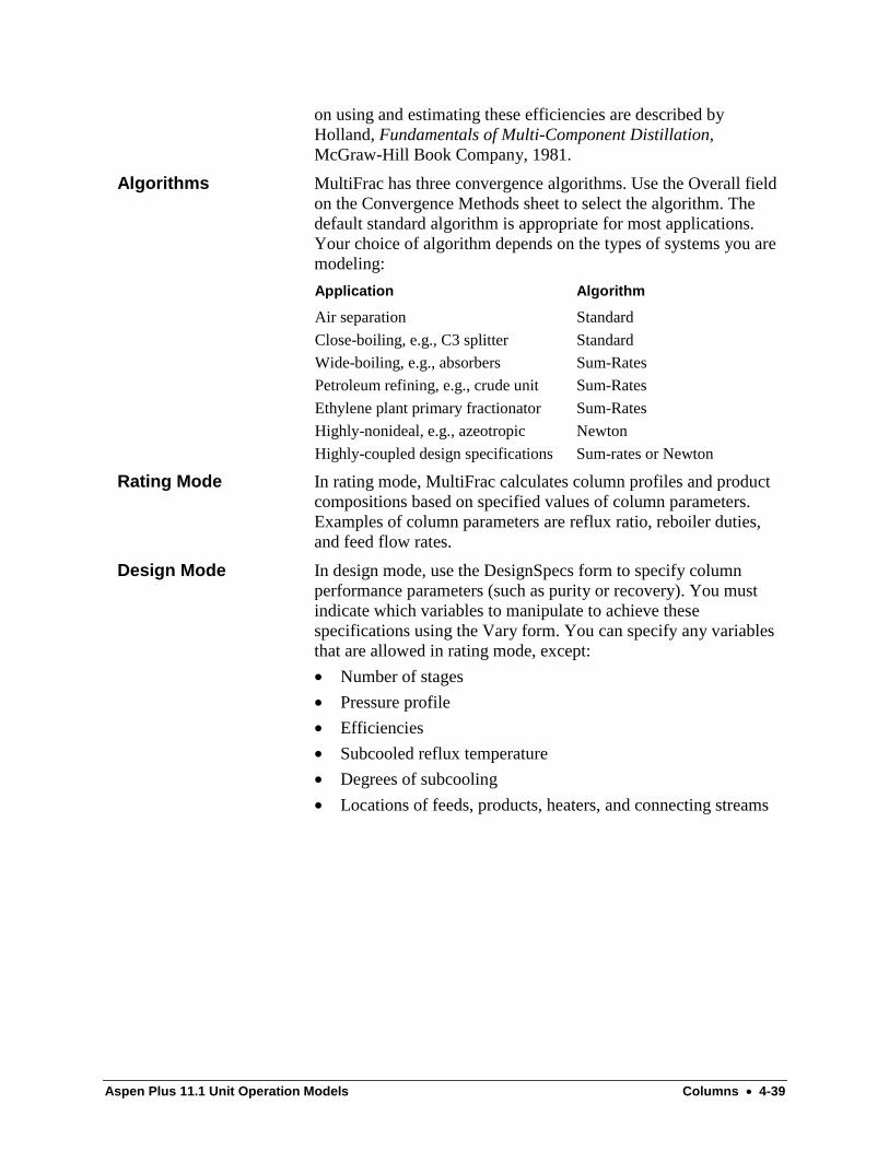
Aspen Plus 11.1 Unit Operation Models Columns • 4-39
on using and estimating these efficiencies are described byHolland, Fundamentals of Multi-Component Distillation,McGraw-Hill Book Company, 1981.
MultiFrac has three convergence algorithms. Use the Overall fieldon the Convergence Methods sheet to select the algorithm. Thedefault standard algorithm is appropriate for most applications.Your choice of algorithm depends on the types of systems you aremodeling:
Application Algorithm
Air separation Standard
Close-boiling, e.g., C3 splitter Standard
Wide-boiling, e.g., absorbers Sum-Rates
Petroleum refining, e.g., crude unit Sum-Rates
Ethylene plant primary fractionator Sum-Rates
Highly-nonideal, e.g., azeotropic Newton
Highly-coupled design specifications Sum-rates or Newton
In rating mode, MultiFrac calculates column profiles and productcompositions based on specified values of column parameters.Examples of column parameters are reflux ratio, reboiler duties,and feed flow rates.
In design mode, use the DesignSpecs form to specify columnperformance parameters (such as purity or recovery). You mustindicate which variables to manipulate to achieve thesespecifications using the Vary form. You can specify any variablesthat are allowed in rating mode, except:
• Number of stages
• Pressure profile
• Efficiencies
• Subcooled reflux temperature
• Degrees of subcooling
• Locations of feeds, products, heaters, and connecting streams
Algorithms
Rating Mode
Design Mode

4-40 • Columns Aspen Plus 11.1 Unit Operation Models
The flow rates of inlet material streams and the duties of inlet heatstreams can also be manipulated variables.
You can specify For any
Purity Stream, including an internalstream †
Recovery of any component groups Set of product streams ††
Flow rate of any component groups Internal stream or set of productstreams
Temperature Stage
Heat duty Stage or connecting stream
Heat duty ratio Stage or connecting stream to anyother stage or connecting stream
Value of any Prop-Set property Internal or product stream †††
Ratio or difference of any pair ofproperties in a Prop-Set
Single or paired internal orproduct stream
Flow ratio of any component groupsto any other component groups
First group can be in any internalstreams ‡
† Express the purity as the sum of mole, mass, or standard liquidvolume fractions of any group of components, relative to any othergroup of components.
†† You can express recovery as a fraction of the same componentsin a subset of the feed stream.
††† See Aspen Plus User Guide, chapter 28.
‡ The second group can be in any other internal streams, or set offeed or product streams.
MultiFrac uses the inside-out approach for column convergence.You can choose from two algorithm variants of this approach:
• Standard
• Sum-rates
To select an algorithm, use the Overall field on the ConvergenceMethods sheet.
The standard algorithm uses the standard inside-out formulationfor the inside loop. It uses either the nested or simultaneousapproach (specified as the Middle loop method on theConvergence Methods sheet) to converge the design specifications.This algorithm is appropriate for most systems.
The sum-rates algorithm uses:
• A sum-rates variant formulation for the inside loop
• The simultaneous approach to converge the designspecifications
Column Convergence

Aspen Plus 11.1 Unit Operation Models Columns • 4-41
Sum-rates is well suited for:
• Wide-boiling systems
• Columns with steep flow gradients
MultiFrac also has the Newton algorithm, which uses a Napthali-Sandholm formulation. It solves the column-describing equationsand design specifications simultaneously, using Newton’s method.This method can enhance convergence for highly-nonidealsystems, such as azeotropic distillation. The Newton algorithm isgenerally slower than the other algorithms.
MultiFrac provides two methods for handling design specificationconvergence:
• Nested middle loop
• Simult middle loop
When you use the nested middle loop method, the algorithmattempts to satisfy the design specifications by determining thevalues of the manipulated variables (within their bounds) thatminimize the weighted sum of squares function:
Φ = −
∑
mmw
G G
G
^
**
2
Where:
m = Design specification number
�G = Calculated value
G = Desired value
G** = Scaling factor
w = Weighting factor
For purity and recovery, �G and G are transformed by taking the
logarithm, and G** is taken as unity.
When you use the simult middle loop method, the followingalgorithm solves the design specification functions simultaneouslywith the column describing equations:
( )F G G Gm m m m= − =� / ** 0
The weighting factor is not available for this method.
You can handle design specification convergence by using eitherscaling factors or weighting factors. The following algorithmattempts to satisfy design specifications by determining the values
Design SpecificationConvergence

4-42 • Columns Aspen Plus 11.1 Unit Operation Models
of the manipulated variables (within their bounds) that minimizethe weighted sum of squares function:
Φ = −
∑
mmw
G G
G
�**
2
Where:
m = Design specification number
�G = Calculated value
G = Desired value
G** = Scaling factor
w = Weighting factor
Use Initialization Method on the Convergence Methods sheet tochoose the initialization method.
MultiFrac has two initialization procedures:
• Standard
• Crude
Standard is appropriate for most systems. You must enter at leastthe top and bottom temperature estimates for each column.
Crude invokes a special initialization procedure designed forpetroleum refining and ethylene plant primary fractionator/quenchtower applications. This procedure is designed for systemsconsisting of a main column connected to any number ofsidestrippers. If you specify the following information on theColumns Setup and/or Columns FlowSpecs forms, you do not needto provide estimates:
• All stripper bottoms flow rates
• Either the distillate or bottoms flow rate of the main column
Otherwise, you must enter at least the top and bottom temperatureestimates for each column. You may enter profile estimates on theColumns Estimates form to enhance convergence. Temperatureestimates are usually adequate. Highly nonideal systems mayrequire composition estimates.
Use the BlockOptions form to override the global physicalproperty method. You can specify a single property method on theBlockOptions form. MultiFrac uses this property method for allstages in all columns.
Use the Columns Properties form to specify physical propertymethods when you use a separate property method for an
Initialization
Physical Properties
Aspen Plus 11.1 Unit Operation Models Columns • 4-43
individual column. You can also split a column into any number ofsegments, each using a different property methods.
MultiFrac can perform free-water calculations. By default,MultiFrac performs free-water calculations for the main columncondenser. The free-water phase, if present, is decanted.
Use the Columns Properties form to request free-water calculationsfor additional stages in any column. You can define additionalwater decant product streams on the InletsOutlets form. You canuse this capability to simulate the primary fractionator/quenchtower combination of an ethylene plant.
MultiFrac handles solids by:
• Temporarily removing all solids from inlet streams
• Performing calculations without solids
• Adiabatically mixing solids removed from inlet streams withmain column liquid bottoms
This calculation approach maintains an overall mass and energybalance around the MultiFrac block. But the bottom stage liquidproduct will not be in exact thermal or phase equilibrium withother bottom stage flows (for example, the bottom stage vaporflow).
MultiFrac has extensive capability to size, rate and performpressure drop calculations for trayed and packed columns. Use thefollowing forms to enter specifications:
• TraySizing
• TrayRating
• PackSizing
• PackRating
See Appendix A of the Unit Operation Models Reference Manualfor details on tray and packing types and correlations.
Free Water Handling
Solids Handling
Sizing and Rating ofTrays and Packings

4-44 • Columns Aspen Plus 11.1 Unit Operation Models
PetroFrac ReferencePetroFrac is a rigorous model designed for simulating all types ofcomplex vapor-liquid fractionation operations in the petroleumrefining industry. Typical operations include:
• Preflash tower
• Atmospheric crude unit
• Vacuum unit
• Catalytic cracker main fractionator
• Delayed coker main fractionator
• Vacuum lube fractionator
You also can use PetroFrac to model the primaryfractionator/quench tower combination in the quench section of anethylene plant. PetroFrac can detect a free-water phase in thecondenser or anywhere in the column. It can decant the free-waterphase on any stage. Although PetroFrac assumes equilibrium stagecalculations, you can specify either Murphree or vaporizationefficiencies. You can use PetroFrac to size and rate columnsconsisting of trays and/or packings. PetroFrac can model bothrandom and structured packings.
Use the following forms to enter specifications and view results ofPetroFrac:
Use this form To do this
Setup Specify basic column configuration andoperating conditions
Pumparounds Specify pumparound specifications and viewresults
Pumparounds Hcurves Specify pumparound heating or cooling curvetables and view tabular results
Strippers Specify parameters and view results of sidestrippers
HeatersCoolers Specify stage heating or cooling specifications
RunbackSpecs Specify runback specification parameters
Efficiencies Specify stage or component efficiencies
DesignSpecs Specify design specifications, manipulatedvariables, and view convergence results
CondenserHcurves Specify condenser heating or cooling curvetables and view tabular results
ReboilerHcurves Specify reboiler heating or cooling curve tablesand view tabular results
Aspen Plus 11.1 Unit Operation Models Columns • 4-45
Use this form To do this
TraySizing Specify sizing calculation parameters for traycolumn sections, and view results
TrayRating Specify rating calculation parameters for traycolumn sections, and view results
PackSizing Specify sizing calculation parameters for packedcolumn sections, and view results
PackRating Specify rating calculation parameters for packedcolumn sections, and view results
Properties Specify physical property parameters forcolumn sections
Estimates Specify estimates for column temperatures andflows
Convergence Specify convergence parameters
Report Specify block-specific report options andpseudostreams
BlockOptions Override global values for physical properties,simulation options, diagnostic message levels,and report options for this block
UserSubroutines Specify user subroutines for tray and packingrating and sizing
Connectivity View stream connectivity for the PetroFracblock
ResultsSummary View key column results for the overallPetroFrac column
Profiles View column profiles
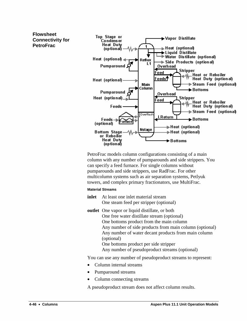
4-46 • Columns Aspen Plus 11.1 Unit Operation Models
PetroFrac models column configurations consisting of a maincolumn with any number of pumparounds and side strippers. Youcan specify a feed furnace. For single columns withoutpumparounds and side strippers, use RadFrac. For othermulticolumn systems such as air separation systems, Petlyuktowers, and complex primary fractionators, use MultiFrac.
Material Streams
inlet At least one inlet material streamOne steam feed per stripper (optional)
outlet One vapor or liquid distillate, or bothOne free water distillate stream (optional)One bottoms product from the main columnAny number of side products from main column (optional)Any number of water decant products from main column(optional)One bottoms product per side stripperAny number of pseudoproduct streams (optional)
You can use any number of pseudoproduct streams to represent:
• Column internal streams
• Pumparound streams
• Column connecting streams
A pseudoproduct stream does not affect column results.
FlowsheetConnectivity forPetroFrac

Aspen Plus 11.1 Unit Operation Models Columns • 4-47
Heat Streams
inlet One heat stream per stage for the main column (optional)One heat stream per pumparound heater/cooler (optional)One heat stream per stripper reboiler (optional)One heat stream per stripper bottom liquid return (optional)
outlet One heat stream per stage for the main column (optional)One heat stream per pumparound heaters/cooler (optional)One heat stream per stripper reboiler (optional)One heat stream per stripper bottom liquid return (optional)
PetroFrac uses an inlet heat stream as a duty specification for allstages except the condenser, reboiler, pumparounds, and stripperbottom liquid return.
If you do not give sufficient operating column specifications on theSetup Configuration sheet, PetroFrac uses a heat stream as aspecification for the condenser and reboiler.
If you do not give two specifications on the PumparoundsSpecifications sheet, PetroFrac uses a heat stream as a specificationfor pumparounds.
If you do not give two specifications for the bottom liquid returnon the Strippers Setup LiquidReturn sheet, PetroFrac uses a heatstream as a specification.
If you give two specifications on the Setup Configuration sheet orPumparounds Specifications sheet, PetroFrac does not use the inletheat stream as a specification. The heat stream supplies therequired heating or cooling.
Use optional outlet streams for the net heat duty of the condenser,reboiler, and pumparounds. The value of the outlet heat streamequals the value of the inlet heat stream (if any) minus the actual(calculated) heat duty.
The main column can have any number of inlet streams. It can alsohave up to three product streams per stage (one vapor, onehydrocarbon liquid, and one free water).
The side strippers can have a steam feed. They must have a liquidbottoms product. You can use a heat stream as the heat source forthe reboiler. If you do not specify the reboiler duty, bottoms flowrate, and steam feed, PetroFrac uses the heat stream as a dutyspecification.
Optionally, the stripper liquid bottoms may be partially returned tothe main column. To specify a bottom liquid return, you must entertwo specifications on the Strippers Setup LiquidReturn sheet.
Main Column
Side Strippers

4-48 • Columns Aspen Plus 11.1 Unit Operation Models
You can specify a feed furnace. A feed furnace can have anynumber of feeds. The vapor and liquid streams from the furnaceare fed to the stage where the furnace is attached.
Within each column or stripper, stages are numbered from the topdown. If present, the main column condenser is stage 1.
You define the main column configuration using Condenser andReboiler on the Setup Configuration sheet. PetroFrac allows sixcondenser types:
• Subcooled
• Total
• Partial with vapor distillate product only
• Partial with both vapor and liquid distillate products
• No condenser, with pumparound to top stage
• No condenser, with external feed to top stage
You can specify one of three reboiler types:
• Kettle reboiler
• No reboiler, with pumparound to bottom stage
• No reboiler, with external feed to bottom stage
The types and number of required operating specifications dependon the column configuration. Normally, you must enter twocolumn operating specifications. If either a condenser or a reboileris absent, you must enter one specification. If both the condenserand reboiler are absent, do not enter any specification.
Use the Setup Streams sheet to specify the feed and product stagelocations. You may also identify a feed as the stripping steam, andoverride its flow by specifying a steam-to-product ratio.
PetroFrac provides three conventions for handling feed streams(see PetroFrac Feed Convention Above-Stage and PetroFrac FeedConvention On-Stage in the following figures):
• Above-Stage
• On-Stage
• Furnace
When Feed-Convention is Above-Stage, PetroFrac introduces amaterial stream between adjacent stages. The liquid portion flowsto the stage (n) you specify. The vapor portion flows to the stageabove (n – 1). You can introduce a liquid feed to the top stage (orcondenser) by specifying Stage=1. You can introduce a vapor feedto the bottom stage (or reboiler) by specifying Stage=Number ofstages+1.
Feed Furnace
Specifying PetroFrac
Main Column
Feed Stream Handling
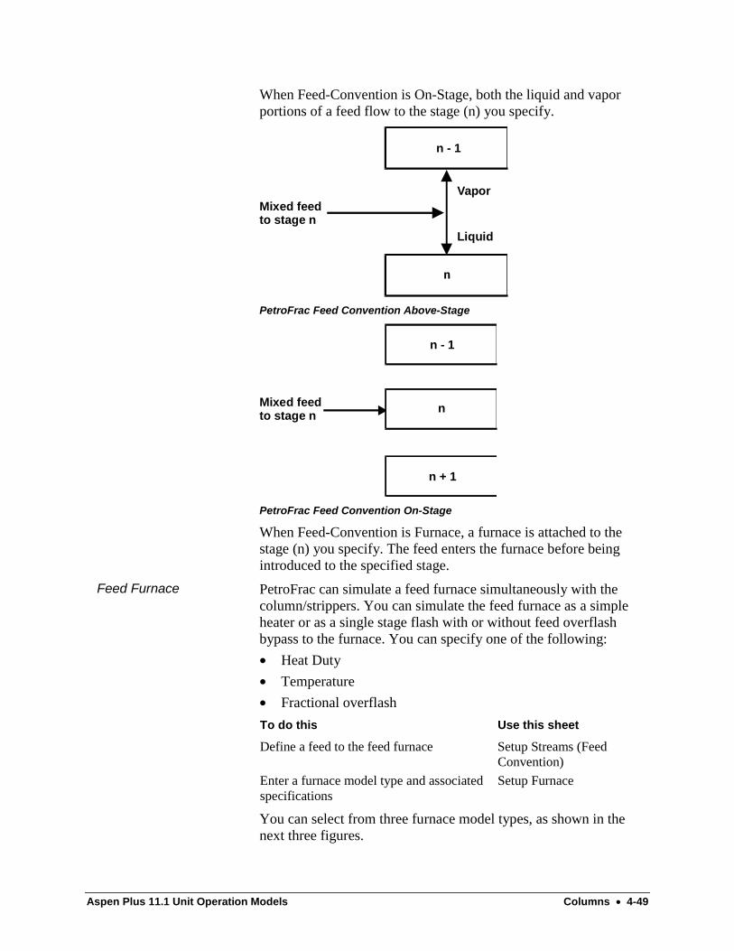
Aspen Plus 11.1 Unit Operation Models Columns • 4-49
When Feed-Convention is On-Stage, both the liquid and vaporportions of a feed flow to the stage (n) you specify.
Vapor
Liquid
n - 1
Mixed feedto stage n
PetroFrac Feed Convention Above-Stage
n - 1
n + 1
nMixed feed to stage n
PetroFrac Feed Convention On-Stage
When Feed-Convention is Furnace, a furnace is attached to thestage (n) you specify. The feed enters the furnace before beingintroduced to the specified stage.
PetroFrac can simulate a feed furnace simultaneously with thecolumn/strippers. You can simulate the feed furnace as a simpleheater or as a single stage flash with or without feed overflashbypass to the furnace. You can specify one of the following:
• Heat Duty
• Temperature
• Fractional overflash
To do this Use this sheet
Define a feed to the feed furnace Setup Streams (FeedConvention)
Enter a furnace model type and associatedspecifications
Setup Furnace
You can select from three furnace model types, as shown in thenext three figures.
Feed Furnace
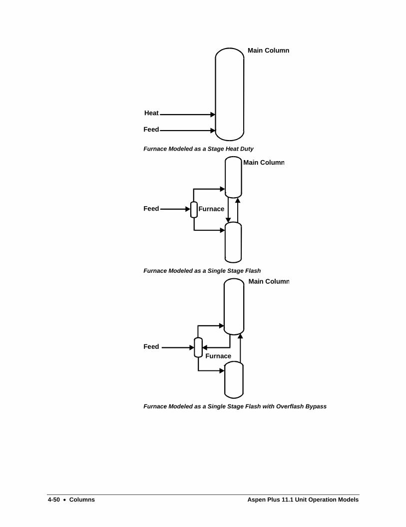
4-50 • Columns Aspen Plus 11.1 Unit Operation Models
Heat
Feed
Main Column
Furnace Modeled as a Stage Heat Duty
Feed Furnace
Main Column
Furnace Modeled as a Single Stage Flash
FeedFurnace
Main Column
Furnace Modeled as a Single Stage Flash with Overflash Bypass
Aspen Plus 11.1 Unit Operation Models Columns • 4-51
If Model= PetroFrac models thefurnace as
And calculates
Heater Stage heat duty on thefeed stage
—
Flash Single-stage flash Furnace temperature, degree ofvaporization, vapor/liquidcompositions
Flash-Bypass Single-stage flash withthe overflash bypassedback to the furnace
Furnace temperature, degree ofvaporization, vapor/liquidcompositions
Use the RunbackSpecs form to specify the flow rate of liquidrunback from any stage. When you enter a liquid runbackspecification, you must allow PetroFrac to adjust one of thefollowing:
• Flow rate of a pumparound
• Duty of an interstage heater/cooler
Use the following sheets to enter specifications for pumparounds.
Use this sheet To enter
PumparoundsSpecifications
Pumparound connectivity and cooler/heaterspecifications
Report PseudoStreams Pseudostream assignment for the pumparound
Hcurves Specifications Heating/cooling curve specifications
Pumparounds are associated with the maincolumn. They can betotal or partial drawoffs of the stage liquid flow. You must specifythe draw and return stage locations for each pumparound. Forpartial drawoffs, you must specify two of the following:
• Flow rate
• Temperature
• Temperature change
• Heat Duty
For total drawoffs, you must specify one of the following:
• Temperature
• Temperature change
• Heat Duty
Use the Stripper forms and sheets to enter specifications for sidestrippers.
Side strippers may be either steam-stripped or reboiled. For steamstrippers, you must enter a steam stream. You can override its flow
Liquid Runbacks
Pumparounds
Side Strippers
4-52 • Columns Aspen Plus 11.1 Unit Operation Models
rate by specifying a steam-to-product ratio. For reboiled strippers,you must specify a reboiler duty.
PetroFrac assumes:
• A liquid draw goes from the main column to the top of thestripper.
• The stripper overhead is returned to the main column.
You must specify the draw and return stage locations. You canalso:
• Return a fraction of the stripper bottoms to the main column
• Specify additional liquid draws from other stages of the maincolumn as feeds to the strippers
PetroFrac supports two kinds of efficiencies: vapor-liquid-equilibrium efficiencies and thermal efficiencies.
Vapor-Liquid-Equilibrium Efficiencies
You can specify one of two types of vapor-liquid-equilibriumefficiencies:
• Vaporization
• Murphree
Vaporization efficiency is defined as:
Effy
K xiv i j
i j i j
= ,
, ,
Murphree efficiency is defined as:
Effy y
k x yi jM i j i j
i j i j i j,
, ,
, , ,
=−−
+
+
1
1
Where:
K = Equilibrium K value
x = Liquid mole fraction
y = Vapor mole fraction
Eff v = Vaporization efficiency
Eff M = Murphree efficiency
i = Component index
j = Stage index
To specify vaporization or Murphree efficiencies, enter the numberof actual stages on the Setup Configuration sheet and StrippersSetup Configuration sheet as Number of stages. Then use the
Efficiencies

Aspen Plus 11.1 Unit Operation Models Columns • 4-53
Efficiencies and Strippers Efficiencies forms to enter theefficiencies.
You can use any of these efficiencies to account for departure fromequilibrium. But you cannot convert from one efficiency to theother. Magnitudes of the efficiencies can be quite different. Detailson using and estimating these efficiencies are described byHolland, Fundamentals of Multi-Component Distillation,McGraw-Hill Book Company, 1981.
Thermal efficiencies
Thermal tray efficiencies are an AspenTech proprietary type ofefficiency used to model the thermal non-equilibrium effects foundin large refinery columns such as crude columns and mainfractionators.
Vapor thermal efficiencies are designed for columns that have highvapor loads such as crude columns, cat cracker, and coker mainfractionators. These columns typically have superheated vaporfeeds and are characterized by high vapor-to-liquid ratios,especially near the bottom of the column. The thermal trayefficiency allows the vapor and liquid temperatures to be different(not at equilibrium), thus allowing for the calculation of both acompositional and a thermal deviation from equilibrium. Incontrast, Murphree tray efficiencies assume thermal equilibriumbetween the vapor and liquid phases.
Thermal tray efficiencies are defined strictly over the range 0.0 to1.0 with 1.0 corresponding to an ideal stage at thermal equilibrium.
Vapor thermal tray efficiencies should be used where high and/orsuperheated vapor flows dominate the column profile. Liquidthermal tray efficiencies should be used in the opposite situationwhere high and/or sub-cooled liquid flows dominate the columnprofile. Only one of these two types of thermal efficiency may beused on any given section of the column.
Thermal tray efficiencies are defined analogously to Murphree trayefficiencies. Murphree tray efficiencies can be used with vapor ofliquid tray efficiencies, but care must be taken to understand therelative effects of the two efficiencies and to ensure thatindependent measurements are used to tune them.
For convergence PetroFrac uses:
• The sum-rates variant of the inside-out algorithm
• A special initialization procedure designed for petroleumrefining applications
Convergence
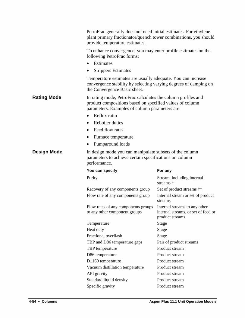
4-54 • Columns Aspen Plus 11.1 Unit Operation Models
PetroFrac generally does not need initial estimates. For ethyleneplant primary fractionator/quench tower combinations, you shouldprovide temperature estimates.
To enhance convergence, you may enter profile estimates on thefollowing PetroFrac forms:
• Estimates
• Strippers Estimates
Temperature estimates are usually adequate. You can increaseconvergence stability by selecting varying degrees of damping onthe Convergence Basic sheet.
In rating mode, PetroFrac calculates the column profiles andproduct compositions based on specified values of columnparameters. Examples of column parameters are:
• Reflux ratio
• Reboiler duties
• Feed flow rates
• Furnace temperature
• Pumparound loads
In design mode you can manipulate subsets of the columnparameters to achieve certain specifications on columnperformance.
You can specify For any
Purity Stream, including internalstreams †
Recovery of any components group Set of product streams ††
Flow rate of any components group Internal stream or set of productstreams
Flow rates of any components groupsto any other component groups
Internal streams to any otherinternal streams, or set of feed orproduct streams
Temperature Stage
Heat duty Stage
Fractional overflash Stage
TBP and D86 temperature gaps Pair of product streams
TBP temperature Product stream
D86 temperature Product stream
D1160 temperature Product stream
Vacuum distillation temperature Product stream
API gravity Product stream
Standard liquid density Product stream
Specific gravity Product stream
Rating Mode
Design Mode

Aspen Plus 11.1 Unit Operation Models Columns • 4-55
You can specify For any
Flash point Product stream
Pour point Product stream
Refractive index Product stream
Reid vapor pressure Product stream
Value of any Prop-Set property Internal or product stream †††
Difference of any pair of Prop-Setproperties
Pair of product streams
Watson UOP K factor Product stream
† Express the purity as the sum of mole, mass, or standard liquidvolume fraction of any group of components relative to any othergroup of components.
†† Express recovery as a fraction of the same components in asubset of feed streams.
††† See Aspen Plus User Guide, Chapter 28.
You can also specify overflash for a furnace feed stream.
Use the BlockOptions form to override the global physicalproperty method. You can specify one method on this form, whichPetroFrac uses for all stages in the main column and strippers.
You can also split the main column or a stripper into any numberof segments, each using a different property method.
Use this sheet When you use different properties for
Properties Property Sections The main column
Strippers Properties PropertySections
A stripper
PetroFrac can perform free-water calculations in the main columnand side strippers. By default, PetroFrac performs free-watercalculations for the main column condenser. The free-water phase,if present, is decanted.
To do this Use these sheets
Request free-water calculationsfor additional stages in the maincolumns and strippers
Properties Freewater StagesStrippers Properties Freewater Stages
Define additional water decantproduct streams for the maincolumn
Setup Streams
PetroFrac handles solids by:
• Temporarily removing all solids from inlet streams
• Performing calculations without solids
Physical Properties
Free Water Handling
Solids Handling
4-56 • Columns Aspen Plus 11.1 Unit Operation Models
• Adiabatically mixing solids removed from inlet streams withmain column liquid bottoms
This calculation approach maintains an overall mass and energybalance around the PetroFrac block. But the bottom stage liquidproduct will not be in exact thermal or phase equilibrium withother bottom stage flows (for example, the bottom stage vaporflow).
PetroFrac has extensive capabilities to size, rate, and performpressure drop calculations for trayed and packed columns. Use thefollowing PetroFrac forms to enter specifications:
• TraySizing, TrayRating, PackSizing, PackRating
• Strippers TraySizing, Strippers TrayRating, StrippersPackSizing, Strippers PackRating
See Appendix A of the Unit Operation Models Reference Manualfor details on tray and packing types and correlations.
The features listed below are not supported in equation-orientedformulation. However, the capabilities are still available for the EOsolution strategy via the Perturbation Layer.
• Feed conventions FURNACE and ABOVE-STAGE
• Multiple feeds to trays
• All Furnace specifications
• Ratio of steam to products specifications
• Additional feed from main column to strippers
• Stage pseudostreams for main shell and strippers with totalliquid/total vapor phase
• Liquid return from strippers to main column
• Free-water stage specifications in the main column or strippers
• TPSAR with pressure update
• Prop-sections
• Features which are globally unsupported
Some features in Petrofrac are not supported in the EOformulation. When these features appear in Petrofrac blocksrunning in EO mode, they are dropped from the problemspecifications with a warning.
• Design specs involving property differences
• Design specs and manipulated variables spanning differentcolumns
Sizing and Rating ofTrays and Packings
EO Usage Notes forPetroFrac
Aspen Plus 11.1 Unit Operation Models Columns • 4-57
RateFrac ReferenceRateFrac is a rate-based nonequilibrium model for simulating alltypes of multistage vapor-liquid fractionation operations. RateFracsimulates actual tray and packed columns, rather than the idealizedrepresentation of equilibrium stages. RateFrac explicitly accountsfor the underlying interphase mass and heat transfer processes todetermine the degree of separation. RateFrac does not useempirical factors such as efficiencies and the Height Equivalent toa Theoretical Plate (HETP).
RateFrac is applicable for:
• Ordinary distillation
• Absorption
• Reboiled absorption
• Stripping
• Reboiled stripping
• Extractive and azeotropic distillation
RateFrac is suitable for:
• Two-phase systems
• Narrow and wide-boiling systems
• Systems exhibiting strong liquid phase nonideality
RateFrac can also detect and handle a free water phase in thecondenser.
RateFrac can model columns with chemical reactions. Reactionsinclude:
• Equilibrium
• Rate-controlled
• Electrolytic
RateFrac models a complex configuration consisting of a singlecolumn or interlinked columns. The configuration may have:
• Any number of columns, each with any number of RateFracSegments
• Any number of connections between columns or within eachcolumn
• Arbitrary flow splitting and mixing of connecting streams
RateFrac can handle operations with:
• Side strippers
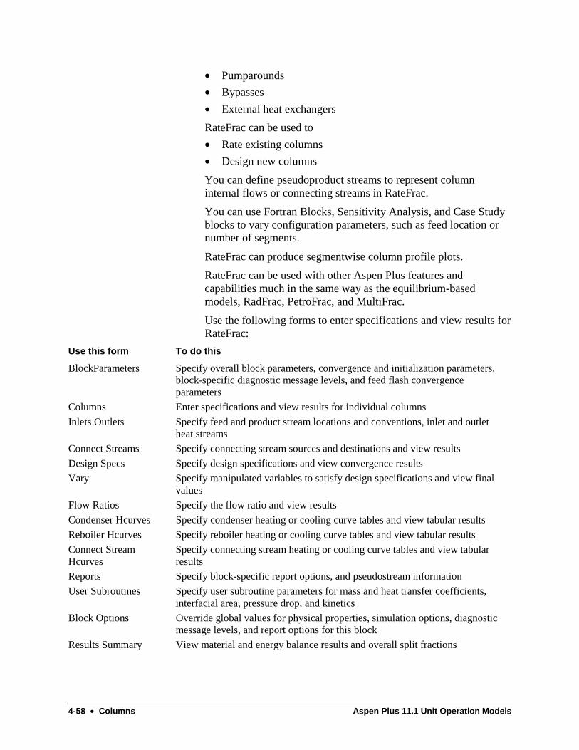
4-58 • Columns Aspen Plus 11.1 Unit Operation Models
• Pumparounds
• Bypasses
• External heat exchangers
RateFrac can be used to
• Rate existing columns
• Design new columns
You can define pseudoproduct streams to represent columninternal flows or connecting streams in RateFrac.
You can use Fortran Blocks, Sensitivity Analysis, and Case Studyblocks to vary configuration parameters, such as feed location ornumber of segments.
RateFrac can produce segmentwise column profile plots.
RateFrac can be used with other Aspen Plus features andcapabilities much in the same way as the equilibrium-basedmodels, RadFrac, PetroFrac, and MultiFrac.
Use the following forms to enter specifications and view results forRateFrac:
Use this form To do this
BlockParameters Specify overall block parameters, convergence and initialization parameters,block-specific diagnostic message levels, and feed flash convergenceparameters
Columns Enter specifications and view results for individual columns
Inlets Outlets Specify feed and product stream locations and conventions, inlet and outletheat streams
Connect Streams Specify connecting stream sources and destinations and view results
Design Specs Specify design specifications and view convergence results
Vary Specify manipulated variables to satisfy design specifications and view finalvalues
Flow Ratios Specify the flow ratio and view results
Condenser Hcurves Specify condenser heating or cooling curve tables and view tabular results
Reboiler Hcurves Specify reboiler heating or cooling curve tables and view tabular results
Connect StreamHcurves
Specify connecting stream heating or cooling curve tables and view tabularresults
Reports Specify block-specific report options, and pseudostream information
User Subroutines Specify user subroutine parameters for mass and heat transfer coefficients,interfacial area, pressure drop, and kinetics
Block Options Override global values for physical properties, simulation options, diagnosticmessage levels, and report options for this block
Results Summary View material and energy balance results and overall split fractions
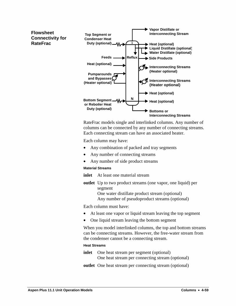
Aspen Plus 11.1 Unit Operation Models Columns • 4-59
1
Vapor Distillate orInterconnecting Stream
Heat (optional)
Heat (optional)
Heat (optional)
Heat (optional)
Liquid Distillate (optional)Water Distillate (optional)
Side Products
Interconnecting Streams (Heater optional)
Bottoms orInterconnecting Streams
Interconnecting Streams (Heater optional)
Reflux
NBottom Segment or Reboiler Heat
Duty (optional)
Top Segment or Condenser Heat
Duty (optional)
Feeds
Pumparoundsand Bypasses
(Heater optional)
RateFrac models single and interlinked columns. Any number ofcolumns can be connected by any number of connecting streams.Each connecting stream can have an associated heater.
Each column may have:
• Any combination of packed and tray segments
• Any number of connecting streams
• Any number of side product streams
Material Streams
inlet At least one material stream
outlet Up to two product streams (one vapor, one liquid) persegmentOne water distillate product stream (optional)Any number of pseudoproduct streams (optional)
Each column must have:
• At least one vapor or liquid stream leaving the top segment
• One liquid stream leaving the bottom segment
When you model interlinked columns, the top and bottom streamscan be connecting streams. However, the free-water stream fromthe condenser cannot be a connecting stream.
Heat Streams
inlet One heat stream per segment (optional)One heat stream per connecting stream (optional)
outlet One heat stream per connecting stream (optional)
FlowsheetConnectivity forRateFrac
4-60 • Columns Aspen Plus 11.1 Unit Operation Models
RateFrac uses an inlet heat stream as a duty specification for allsegments except the condenser, reboiler, and connecting streams.If you do not provide two column operating specifications on theColumns Setup Configuration sheet, RateFrac uses a heat stream asa specification for the condenser and reboiler.
If you do not provide two specifications on the ConnectStreamsInput sheet, RateFrac uses a heat stream as a specification forconnecting streams.
If you provide two specifications on the Columns SetupConfiguration sheet or ConnectStreams Input sheet, RateFrac doesnot use the inlet heat stream as a specification. The inlet heatstream supplies the required heating or cooling.
You can use optional outlet heat streams for the net heat duty ofthe condenser, reboiler, and connecting streams. The value of theoutlet heat stream equals the value of the inlet heat stream (if any),minus the actual (calculated) heat duty.
Most models available for simulating and designingmulticomponent, multistage separation processes are based on theidealized concept of equilibrium or theoretical stages. Thisapproach assumes that the liquid and vapor phases leaving anystage are in thermodynamic equilibrium with each other. The phasecompositions, temperature, and vapor and liquid flow profiles arecalculated by solving the governing material balances, energybalances, and equilibrium relations for each stage.
In practice, columns rarely operate under thermodynamicequilibrium conditions. Vapor-liquid equilibrium prevails only atthe interface separating vapor and liquid phases. The separationachieved in a multistage column depends on the interphase massand heat transfer rate processes. Multicomponent mass transferinteractions can also have pronounced effects on the separation.
When the equilibrium approach is used to model a tray column, acorrection factor (referred to as an efficiency) attempts to accountfor the departure from equilibrium. Many definitions for efficiencyexist, with wide variations in complexity and accuracy. In general,efficiencies depend on:
• Physical characteristics of the equipment, such as columnconfiguration
• Hydrodynamics of the column
• Fluid properties of the system
Murphree vapor efficiencies are the most widely used. Theseefficiencies generally vary from stage to stage within a column,and from component to component. For multicomponent systems,
The Rate-BasedModeling Concept

Aspen Plus 11.1 Unit Operation Models Columns • 4-61
there are no theoretical limitations on Murphree efficiencies.Experimental evidence shows that component efficiencies:
• May vary strongly from component to component
• Can take any value including negative values
Methods used to calculate component efficiencies generally do notinclude the effect of the departure from thermal equilibrium.
Packed columns are also designed using the equilibrium stageconcept. However, HETP is commonly used in place ofefficiencies. HETP varies with:
• Type and size of the packing
• Hydrodynamics of the column
• Fluid properties of the system
Like efficiencies, HETPs may vary strongly from point to pointwithin a column and from system to system.
RateFrac is based on a fundamental and rigorous approach. Thisapproach avoids uncertainties that result when the equilibriumapproach is used with estimated efficiencies or HETP. RateFracdirectly includes mass and heat transfer rate processes in thesystem of equations representing the operation of separationprocess units. RateFrac:
• Describes the simultaneous mass and heat transfer ratephenomena
• Accounts for the multicomponent interactions betweensimultaneously diffusing species
For nonreactive systems, RateFrac comprises:
• Mass and heat balances around vapor and liquid phases
• Mass and heat transfer rate models to determine interphasetransfer rates
• Vapor-liquid equilibrium relations applied at interfacialconditions
• Correlations to estimate mass and heat transfer coefficients andinterfacial areas
For chemically reactive systems, RateFrac includes equations toaccount for the influence of chemical reactions on heat and masstransfer rate processes. For systems involving equilibriumreactions, RateFrac includes equations to represent the chemicalequilibrium conditions.
RateFrac completely avoids the need for efficiencies in traycolumns or HETPs in packed columns. RateFrac has far greaterpredictive capabilities than the conventional equilibrium model.
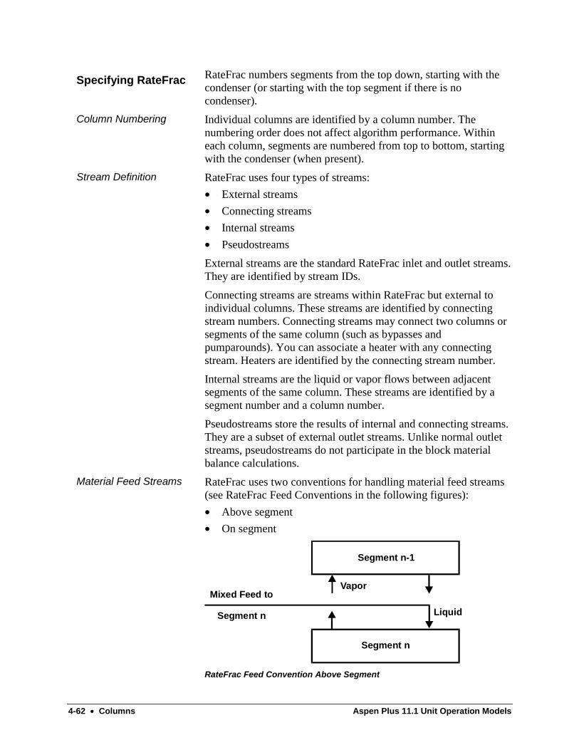
4-62 • Columns Aspen Plus 11.1 Unit Operation Models
RateFrac numbers segments from the top down, starting with thecondenser (or starting with the top segment if there is nocondenser).
Individual columns are identified by a column number. Thenumbering order does not affect algorithm performance. Withineach column, segments are numbered from top to bottom, startingwith the condenser (when present).
RateFrac uses four types of streams:
• External streams
• Connecting streams
• Internal streams
• Pseudostreams
External streams are the standard RateFrac inlet and outlet streams.They are identified by stream IDs.
Connecting streams are streams within RateFrac but external toindividual columns. These streams are identified by connectingstream numbers. Connecting streams may connect two columns orsegments of the same column (such as bypasses andpumparounds). You can associate a heater with any connectingstream. Heaters are identified by the connecting stream number.
Internal streams are the liquid or vapor flows between adjacentsegments of the same column. These streams are identified by asegment number and a column number.
Pseudostreams store the results of internal and connecting streams.They are a subset of external outlet streams. Unlike normal outletstreams, pseudostreams do not participate in the block materialbalance calculations.
RateFrac uses two conventions for handling material feed streams(see RateFrac Feed Conventions in the following figures):
• Above segment
• On segment
Segment n-1
Mixed Feed to
Segment n
Segment n
Vapor
Liquid
RateFrac Feed Convention Above Segment
Specifying RateFrac
Column Numbering
Stream Definition
Material Feed Streams

Aspen Plus 11.1 Unit Operation Models Columns • 4-63
Segment n-1
Mixed Feed to
Segment nSegment n
Segment n + 1
Vapor
Liquid
RateFrac Feed Convention On Segment
When the feed convention is defined as Above segment, RateFracintroduces a material stream between adjacent segments. Theliquid portion flows to segment n, specified as the feed segment.The vapor portion flows to the segment above (segment n-1 in thefigure RateFrac Feed Convention Above segment). You canintroduce a liquid to the top segment (or condenser) by specifyingSegment=1. You can introduce a vapor feed to the bottom segment(or reboiler), by specifying the segment equal to the last segment inthe column +1. When a two-phase feed stream is fed to segment 1,the vapor phase is combined directly with the vapor distillate.Similarly, when a two-phase feed stream is fed to the last segmentof that column + 1, the liquid phase is combined directly with theliquid bottoms product.
When the feed convention is defined as On segment, both theliquid and vapor portions of the feed flow to segment specified(segment n in the previous figure RateFrac Feed Convention Onsegment).
RateFrac assumes that a vapor feed (or the vapor portion of amixed feed) combines with the vapor phase in the segment itenters. RateFrac also assumes that a liquid feed (or the liquidportion of a mixed feed) combines with the liquid phase in thesegment it enters.
Specify the column configuration by indicating the following onthe Columns Configuration sheet:
• Number of segments
• Presence or absence of condensers and reboilers
• Equilibrium and nonequilibrium segments
Column Configuration

4-64 • Columns Aspen Plus 11.1 Unit Operation Models
RateFrac allows any number of connecting streams. Any numberof these streams can have the same:
• Source column, segment, and phase
• Destination column and segment
RateFrac introduces connecting streams on the destination segmentregardless of their phase (Convention = On Segment). Allconnecting streams can have a heater. Enter all specifications forconnecting streams on the ConnectStreams Input sheet. RateFracdoes not allow phase change for connecting streams.
Connecting streams can be either a total or a partial drawoff of thesegment flow. Enter the required specifications as follows:
If the drawoff type is You enter
Partial Two of the following: flow, temperature ortemperature change and heat duty †
Total One of the following: temperature or temperaturechange and heat duty ††
† Enter zero for heat duty if heater is absent.
†† Enter zero for heat duty if heater is absent. Flow is taken as thenet flow of the segment, excluding any product flow and any otherconnecting stream flow.
You must specify the total number of columns and connectingstreams.
Use this form To enter Such as
ColumnsTraySpecs
Tray specifications Number of trays orNumber of trays per segmentTray typeTray characteristics
ColumnsPackSpecs
Packingspecifications
Total height of packing orHeight of packing per segmentPacking typePacking characteristics
You must also specify:
• Inlet stream locations
• Heat stream locations, heat duty, and phase
• Pressure profile for each column
• Condenser type
• Two operating specifications for multisegment columns andone for single-segment columns
• Source and destination of any connecting stream and associatedheater specifications
Connecting Streams
Required Specifications
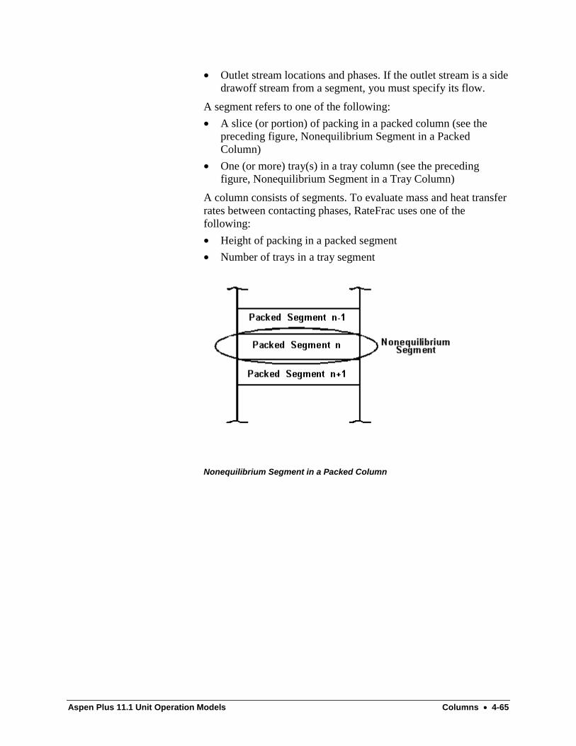
Aspen Plus 11.1 Unit Operation Models Columns • 4-65
• Outlet stream locations and phases. If the outlet stream is a sidedrawoff stream from a segment, you must specify its flow.
A segment refers to one of the following:
• A slice (or portion) of packing in a packed column (see thepreceding figure, Nonequilibrium Segment in a PackedColumn)
• One (or more) tray(s) in a tray column (see the precedingfigure, Nonequilibrium Segment in a Tray Column)
A column consists of segments. To evaluate mass and heat transferrates between contacting phases, RateFrac uses one of thefollowing:
• Height of packing in a packed segment
• Number of trays in a tray segment
Nonequilibrium Segment in a Packed Column
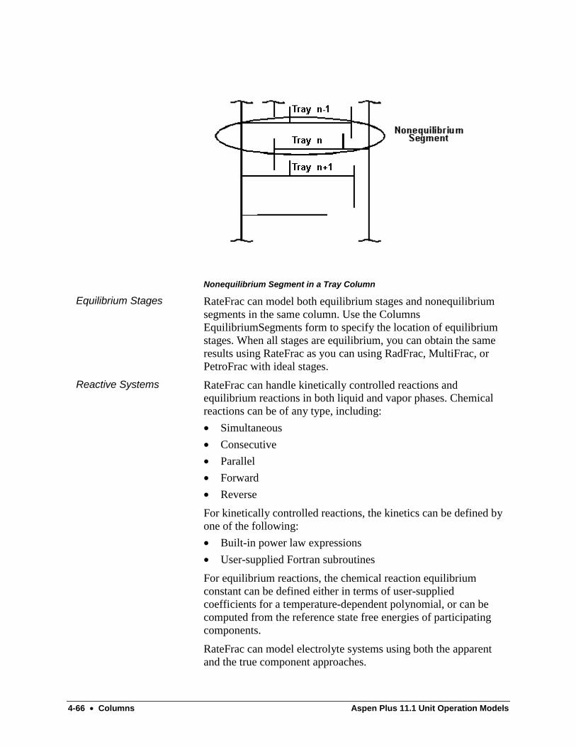
4-66 • Columns Aspen Plus 11.1 Unit Operation Models
Nonequilibrium Segment in a Tray Column
RateFrac can model both equilibrium stages and nonequilibriumsegments in the same column. Use the ColumnsEquilibriumSegments form to specify the location of equilibriumstages. When all stages are equilibrium, you can obtain the sameresults using RateFrac as you can using RadFrac, MultiFrac, orPetroFrac with ideal stages.
RateFrac can handle kinetically controlled reactions andequilibrium reactions in both liquid and vapor phases. Chemicalreactions can be of any type, including:
• Simultaneous
• Consecutive
• Parallel
• Forward
• Reverse
For kinetically controlled reactions, the kinetics can be defined byone of the following:
• Built-in power law expressions
• User-supplied Fortran subroutines
For equilibrium reactions, the chemical reaction equilibriumconstant can be defined either in terms of user-suppliedcoefficients for a temperature-dependent polynomial, or can becomputed from the reference state free energies of participatingcomponents.
RateFrac can model electrolyte systems using both the apparentand the true component approaches.
Equilibrium Stages
Reactive Systems

Aspen Plus 11.1 Unit Operation Models Columns • 4-67
Enter the following information on the Reactions form:
• Reaction stoichiometry
• Reaction type
• Phase in which reactions occur
Depending on the reaction type, you must enter either theequilibrium constant or kinetic parameters. For electrolyticreactions, you can also enter the reaction data on the Chemistryform.
To associate reactions with a column segment, enter thecorresponding Reactions ID (or Chemistry ID or User ReactionsID) on the Columns Reactions Specifications sheet.
For rate-controlled reactions, you must enter holdup data for thephase where reactions occur.
For thesesegments
Use this form to enter holdup information
Equilibrium Columns Reactions
Tray Columns TraySpecs
Packed Columns PackSpecs
Use the Columns HeatersCoolers Side Duties sheet to specify:
• Heat duty for a segment
• Heater segment location (column and segment)
• Phase
Use the Columns HeatersCoolers Utility Exchangers sheet tospecify cooling (or heating) of any segment using a coolant (orheating fluid).
You can use a heat stream to provide heat integration. Heatintegration occurs when the duty recovered from another block isused as the heat source of heaters and coolers. Enter heat streamdata on the InletsOutlets Heat Streams sheet.
Use the RateFrac BlockOptions form to override the globalphysical property property method. You can specify only oneproperty method on the BlockOptions form. RateFrac uses thisproperty method for the whole column. RateFrac does not allowmultiple physical property methods.
RateFrac can perform free-water calculations only in condensers.
In rating mode, RateFrac calculates temperatures, flows, and molefraction profiles based on specified values of column parameterssuch as:
• Reflux ratio
• Product flows
Heaters and Coolers
Physical PropertySpecifications
Handling Free Water
Rating Mode
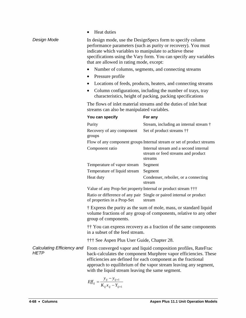
4-68 • Columns Aspen Plus 11.1 Unit Operation Models
• Heat duties
In design mode, use the DesignSpecs form to specify columnperformance parameters (such as purity or recovery). You mustindicate which variables to manipulate to achieve thesespecifications using the Vary form. You can specify any variablesthat are allowed in rating mode, except:
• Number of columns, segments, and connecting streams
• Pressure profile
• Locations of feeds, products, heaters, and connecting streams
• Column configurations, including the number of trays, traycharacteristics, height of packing, packing specifications
The flows of inlet material streams and the duties of inlet heatstreams can also be manipulated variables.
You can specify For any
Purity Stream, including an internal stream †
Recovery of any componentgroups
Set of product streams ††
Flow of any component groups Internal stream or set of product streams
Component ratio Internal stream and a second internalstream or feed streams and productstreams
Temperature of vapor stream Segment
Temperature of liquid stream Segment
Heat duty Condenser, reboiler, or a connectingstream
Value of any Prop-Set property Internal or product stream †††
Ratio or difference of any pairof properties in a Prop-Set
Single or paired internal or productstream
† Express the purity as the sum of mole, mass, or standard liquidvolume fractions of any group of components, relative to any othergroup of components.
†† You can express recovery as a fraction of the same componentsin a subset of the feed stream.
††† See Aspen Plus User Guide, Chapter 28.
From converged vapor and liquid composition profiles, RateFracback-calculates the component Murphree vapor efficiencies. Theseefficiencies are defined for each component as the fractionalapproach to equilibrium of the vapor stream leaving any segment,with the liquid stream leaving the same segment.
Effy y
K x Yijij ij
ij ij ij
=−−
+
+
1
1
Design Mode
Calculating Efficiency andHETP

Aspen Plus 11.1 Unit Operation Models Columns • 4-69
Where:
Eff = Murphree vapor efficiency
K = Vapor-liquid equilibrium K value
x = Liquid mole fraction
y = Vapor mole fraction
i = Component index
j = Segment index
For each segment of packed columns, RateFrac calculates thefractional approach to equilibrium using the same definition asused for Murphree vapor efficiency. RateFrac reports the height ofpacking required to achieve equilibrium as the HETP for thatsegment.
RateFrac must solve many more equations for a given column thanan equilibrium model. Computing times for RateFrac are greaterthan they are for equilibrium models, particularly for problemscontaining many components. The solution algorithm RateFracuses is an efficient, Newton-based simultaneous correctionapproach. RateFrac solution times increase with the square of thenumber of components. Solution times can be an order ofmagnitude greater than RadFrac, MultiFrac, or PetroFrac solutiontimes for the same problems.
RateFrac uses well-known and accepted correlations to calculate:
• Binary mass transfer coefficients for the vapor and liquid phase
• Interfacial areas
In general, these quantities depend on column diameter andoperating parameters such as:
• Vapor and liquid flow
• Densities
• Viscosities
• Surface tension of liquid
• Vapor and liquid phase binary diffusion coefficients
Mass transfer coefficients and interfacial areas depend on:
Packing characteristics Tray characteristics
Type (random or structured) Type (sieve, valve, or bubble-cap)
Size Weir and flow path length
Specific surface area Downcomer area
Material of construction Weir height
Convergence andComputing Time
References for Built-InCorrelations
4-70 • Columns Aspen Plus 11.1 Unit Operation Models
The correlations involve well-defined dimensionless groups, suchas the Reynolds, Froude, Weber, Schmidt, and Sherwood numbers.The correlations have been fitted to experimental measurementsfrom laboratory and pilot plant absorption and distillation columns.
The correlations RateFrac uses for mass transfer coefficients andinterfacial areas are:
Column type Correlation used
Packed Columns (random packing) Onda et al. (1968)
Packed Columns (structured) Bravo et al. (1985, 1992)
Sieve Trays † Chan and Fair (1984)
Valve Trays Scheffe and Weiland (1987)
Bubble-Cap Trays † Grester et al. (1958)
† These correlations do not provide the mass transfer coefficientsand interfacial areas separately.
RateFrac allows you to write Fortran subroutines to calculate:
• Binary mass transfer coefficients
• Heat transfer coefficients
• Interfacial areas
The subroutines are described in the Aspen Plus User Modelsreference manual.
By applying a rigorous multicomponent mass transfer theory(Krishna and Standart, 1976), RateFrac uses binary mass transfercoefficients to evaluate:
• Multicomponent binary mass transfer coefficients
• Component mass transfer rates between vapor and liquidphases
RateFrac calculates the vapor phase and liquid phase heat transfercoefficients using the Chilton-Colburn analogy (King, 1980). Thisanalogy relates:
• Mass transfer coefficients
• Heat transfer coefficients
• Schmidt number
• Prandtl number

Aspen Plus 11.1 Unit Operation Models Columns • 4-71
RateFrac uses several mass and heat transfer correlations:
• Packed column mass transfer coefficients
• Valve Tray column mass transfer coefficients
• Bubble-Cap Tray column mass transfer coefficients
• Sieve Tray column mass transfer coefficients
• Heat transfer coefficients
RateFrac calculates the mass transfer coefficients and theinterfacial area available for mass transfer using the correlationsdeveloped by Onda et al., 1968.
The correlation for the liquid phase binary mass transfercoefficients is:
( ) ( )kg
L
aSc a dL
in
L
L LinL
p p
ρµ µω
=
−1 3 2 3
1 2 0 4
0 0051
/ // .
.
The correlation for the gas phase binary mass transfer coefficientis:
( ) ( )kRT
a D
G
a uSc a dg
in
g
p in p ging
p p
=
−5 23
0 7
1 3 2
.
.
/
The interfacial area available for mass transfer is given by thecorrelation:
( )[ ]{ }a a Re Fr Wep L L L cω σ σ= − − − −1 145
0 1 0 05 0 2 0 75exp .
. . . .
Where:
ReL
aLp L
=µ
, Fr
a L
gLL
= ρ
ρ
2
2
, We
L
aLp L
=2
σρ
and:
k L
in
= Binary mass transfer coefficient for the binarypair i and n in the liquid phase (m/sec)
ρL = Density of liquid (kg/m3)
g = Acceleration due to gravity (m/sec2
)
µ L = Viscosity of liquid (Newton-sec/m2
)
L = Liquid superficial mass velocity (kg/m2
/sec)
aw = Wetted interfacial area (m2
interfacial area/m3
packing volume)
Mass and HeatTransfer Correlations
Packed Column

4-72 • Columns Aspen Plus 11.1 Unit Operation Models
Sc L
in
= Schmidt number for the binary pair i and n in
the liquid phase = ( )µ ρL L inLD
D L
in
= Binary Maxwell-Stefan diffusion coefficient
for the binary pair i and n (m2
/sec)
ap = Specific surface area of the packing
dp = Nominal diameter of packing or packing size(m)
k g
in
= Binary mass transfer coefficient for the binarypair i and n in the vapor phase (kg
mole/atm/m2
/sec)
R = Universal gas constant (m3atm/kg mole/K)
Tg = Gas phase temperature (K)
G = Gas superficial mass velocity (kg/m2
/sec)
µ g = Viscosity of gas mixture (Newton-sec/m2
)
Sc g
in
= Gas phase Schmidt number for the binary pair
i and n = ( )µ ρg g in
gD
ρg = Density of gas mixture (kg/m3)
D g
in
= Gas-phase binary Maxwell-Stefan diffusion
coefficient for the binary pair i and n (m2
/sec)
σ = Surface tension (Newton/m)
σ c = Critical surface tension of the packing material(Newton/m)
RateFrac calculates the mass transfer coefficients and theinterfacial area available for mass transfer using the correlationsdeveloped by Scheffe and Weiland, 1987.
The correlation for the liquid phase binary mass transfercoefficient is:
( ) ( ) ( ) ( )Sh Re Re v ScinL
g L inL= 1254
0 68 0 09 0 05 0 5.
. . . .
The correlation for the gas phase binary mass transfer coefficientsis:
( ) ( ) ( ) ( )Sh Re Re Scing
g L ing= 9 93
0 87 0 13 0 39 0 5.
. . . .ϖ
Valve Tray Column

Aspen Plus 11.1 Unit Operation Models Columns • 4-73
The interfacial area available for mass transfer is given by thecorrelation:
( ) ( ) ( )a Reg L= 0 270 37 0 25 0 52.
. . .Re ϖ
Where:
Shk ad
DinL
L
in
L
L
in
=ρ
,
Shk ad
Ding
g
in
g
g
in
=ρ
,
ScD
inL L
LL
in
=µ
ρ,
ScD
ing g
gg
in
=µ
ρ,
ReLd
LL
=µ ,
ReGd
gg
=µ
, ϖ =
W
d
and:
L = Liquid mass velocity (kg/m2
/sec) (Velocity isbased on tower active area.)
d = Geometric parameter of unit length (m)
µ L = Viscosity of liquid mixture (Newton-sec/m2
)
G = Gas mass velocity (kg/m2
/sec) (Velocity isbased on tower active area.)
µ g = Viscosity of gas mixture (Newton-sec/m2
)
k L
in
= Binary mass transfer coefficient for the binary
pair i and n in the liquid phase (kg mole/m2
/sec)
a = Interfacial area (m2
interfacial area/m2
toweractive area)
ρL
= Molar density of liquid (kg mole/m3)
D L
in
= Binary Maxwell-Stefan diffusion coefficient
for the binary pair i and n (m2
/sec)
k g
in
= Binary mass transfer coefficient for the binary
pair i and n in the vapor phase (kg mole/m2
/sec)
ρg
= Molar density of gas mixture (kg mole/m3)
D g
in
= Gas-phase binary Maxwell-Stefan diffusion
coefficient for the binary pair i and n (m2
/sec)
ρL = Density of liquid mixture (kg/m3)

4-74 • Columns Aspen Plus 11.1 Unit Operation Models
ρg = Density of gas mixture (kg/m3)
W = Weir height (m)
RateFrac calculates the product of the binary mass transfercoefficients and interfacial areas using the correlations developedby Grester et al., 1958.
The product of liquid phase binary mass transfer coefficients andinterfacial area is given by the correlation:
( ) )k a D F LtL
in inL
L= × +4127 10 0 21313 0158 0 5. ( . .
.
The product of gas phase binary mass transfer coefficient andinterfacial area is given by the correlation:
( )( )k a
h F Q
ScGg
in
w L
ing
=+ − +0 776 4 567 0 2377 104 85
0 5
. . . ..
Where:
k L
in
= Binary mass transfer coefficient for the binary
pair i and n in the liquid phase (kg mole/m2
/sec)
a = Interfacial area (m2
interfacial area/m2
toweractive area)
D L
in
= Binary Maxwell-Stefan diffusion coefficient
for the binary pair i and n (m2
/sec)
F =F-Factor =
µ ρg g1 2/ kg / sec / m1/2 1/2
µ g = Gas volumetric flow per unit active area (m3
/sec/m2
)
ρg = Density of gas mixture (kg/m3)
L = Liquid molar velocity (kg mole/m2
/sec)(Velocity is based on active area.)
tL = Liquid residence time = 0 9998. / (sec)h Z QL L L
hL = Liquid holdup =0 04191 0 19 2 0 0135. . .4545 . ( )+ + −h Q F mw L
ZL = Liquid flow path length (m)
QL = Liquid flow per average path width (m3
/sec/m)
Bubble-Cap Tray Column
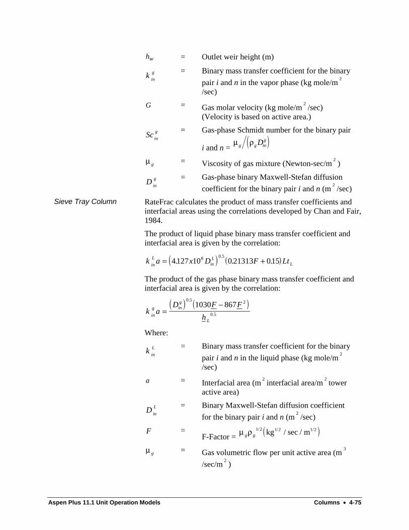
Aspen Plus 11.1 Unit Operation Models Columns • 4-75
hw = Outlet weir height (m)
k g
in
= Binary mass transfer coefficient for the binary
pair i and n in the vapor phase (kg mole/m2
/sec)
G = Gas molar velocity (kg mole/m2
/sec)(Velocity is based on active area.)
Sc g
in
= Gas-phase Schmidt number for the binary pair
i and n = ( )µ ρg g in
gD
µ g = Viscosity of gas mixture (Newton-sec/m2
)
D g
in
= Gas-phase binary Maxwell-Stefan diffusion
coefficient for the binary pair i and n (m2
/sec)
RateFrac calculates the product of mass transfer coefficients andinterfacial areas using the correlations developed by Chan and Fair,1984.
The product of liquid phase binary mass transfer coefficient andinterfacial area is given by the correlation:
( ) ( )k a x D F LtL
in inL
L= +4127 10 0 21313 0158 0 5. . .
.
The product of the gas phase binary mass transfer coefficient andinterfacial area is given by the correlation:
( ) ( )k a
D F F
hg
in
ing
L
=−
0 5 2
0 5
1030 867.
.
Where:
k L
in
= Binary mass transfer coefficient for the binary
pair i and n in the liquid phase (kg mole/m2
/sec)
a = Interfacial area (m2
interfacial area/m2
toweractive area)
D L
in
= Binary Maxwell-Stefan diffusion coefficient
for the binary pair i and n (m2
/sec)
F =F-Factor =
( )µ ρg g1 2 1 2 1 2/ / // /kg sec m
µ g = Gas volumetric flow per unit active area (m3
/sec/m2
)
Sieve Tray Column

4-76 • Columns Aspen Plus 11.1 Unit Operation Models
ρg = Density of gas mixture (kg/m3)
L = Liquid molar velocity (kg mole/m2
/sec)(Velocity is based on active area.)
t L = Liquid residence time = 0 9998. / (sec)h Z QL L L
hL = 0 04191 0 19 2 0 0135. . .4545 . ( )+ + −h Q F mw L
ZL = Liquid flow path length (m)
QL = Liquid flow per average path width
(m3/sec/m)
hw = Outlet weir height (m)
k g
in
= Binary mass transfer coefficient for the binarypair i and n in the vapor phase (m/sec)
D g
in
= Binary Maxwell-Stefan diffusion coefficient
for the binary pair i and n (m2
/sec)
F = Fractional approach to flooding gas velocity =µ µg g F/
µ g F = Gas velocity through active area at flooding(m/sec)
h L = Liquid height =
( ) ( )Γ Γ Γe w e L eh B Q+ 15332 3
//
m
Γe = ( )exp . .− 12 55 0 91Ks
B = ( )0 0327 0 0286 137 8. . exp .+ − hω
Ks = ( ) ( )µ ρ ρ ρg g L g( ) / sec.
−0 5
m
ρL = Density of liquid mixture (kg/m3)
RateFrac calculates the heat transfer coefficients, using theChilton-Colburn analogy (King, 1980).
The heat transfer coefficient is given by:
( )k Sch
Cpavtc
mix
2 3/ =
Where:
k av = Average binary mass transfer coefficients(kg mole/sec)
Sc = Schmidt number
Heat TransferCoefficients
Aspen Plus 11.1 Unit Operation Models Columns • 4-77
htc = Heat transfer coefficient (Watts/K)
Cpmix = Molar heat capacity (Joules/kg mole/K)
Pr = Prandtl number
Bravo, J.L., Rocha, J.A., and Fair, J.R., "Mass Transfer in GauzePackings", Hydrocarbon Processing, January, 91 (1985).
Bravo, J.L., Rocha, J.A., and Fair, J.R., "A Comprehensive Modelfor the Performance of Columns Containing Structured Packings",ICHEME Symposium Series, 128, A439 (1992).
Chan, H. and Fair, J.R., "Prediction of Point Efficiencies in SieveTrays: 1. Binary Systems, 2. Multicomponent Systems," Ind. Eng.Chem. Process Des. Dev., 23, (1984) p. 814.
Grester, J.A., Hill, A.B., Hochgraf, N.N., and Robinson, D.G.,"Tray Efficiencies in Distillation Columns," AIChE Report,(1958).
King, C.J., Separation Processes, Second Edition, McGraw-HillCompany, (1980).
Krishna, R. and Standart, G.L., "A Multicomponent Film ModelIncorporating a General Matrix Method of Solution to theMaxwell-Stefan Equations," AIChE J., 22, (1976) p. 383.
Onda, K., Takeuchi, H., and Okumoto, Y., "Mass TransferCoefficients between Gas and Liquid Phases in Packed Columns,"J. Chem. Eng., Japan, 1, (1968) p. 56.
Perry, R.H. and Chilton, C.H., "Chemical Engineers’ Handbook,"Fifth Edition, McGraw-Hill Book Company, Section 18 (1973).
Scheffe, R.D. and Weiland, R.H., "Mass Transfer Characteristicsof Valve Trays," Ind. Eng. Chem. Res., 26, (1987) p. 228.
References
4-78 • Columns Aspen Plus 11.1 Unit Operation Models
BatchFrac ReferenceBatchFrac is a batch distillation model that solves unsteady-stateheat and material balance equations. These equations describe thebehavior of a multi-stage batch distillation column. BatchFracapplies rigorous heat balances, material balances, and equilibriumrelationships at each stage. BatchFrac calculates the profiles ofcolumn composition, temperature, pressure, and vapor and liquidflows as a function of time.
BatchFrac can model the following systems:
• Narrow-boiling
• Wide-boiling
• Strong liquid phase nonideality
• Three-phase
• Reactive
BatchFrac assumes:
• Equilibrium stages
• Constant liquid holdup and zero vapor holdup
BatchFrac can handle:
• Continuous feeds to the column
• Continuous sideproduct withdrawal
• Nonadiabatic column operation
• Interstage heaters and coolers
• Vaporization efficiencies for modeling nonequilibrium stages
BatchFrac can also handle the presence of:
• A free-water phase in the condenser
• Two liquid phases in the condenser
BatchFrac does not model column hydraulics.
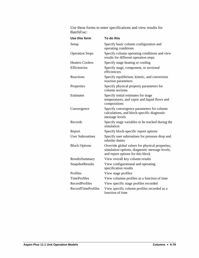
Aspen Plus 11.1 Unit Operation Models Columns • 4-79
Use these forms to enter specifications and view results forBatchFrac:
Use this form To do this
Setup Specify basic column configuration andoperating conditions
Operation Steps Specify column operating conditions and viewresults for different operation steps
Heaters Coolers Specify stage heating or cooling
Efficiencies Specify stage, component, or sectionalefficiencies
Reactions Specify equilibrium, kinetic, and conversionreaction parameters
Properties Specify physical property parameters forcolumn sections
Estimates Specify initial estimates for stagetemperatures, and vapor and liquid flows andcompositions
Convergence Specify convergence parameters for columncalculations, and block-specific diagnosticmessage levels
Records Specify stage variables to be tracked during thesimulation
Report Specify block-specific report options
User Subroutines Specify user subroutines for pressure drop andreboiler duties
Block Options Override global values for physical properties,simulation options, diagnostic message levels,and report options for this block
ResultsSummary View overall key column results
SnapshotResults View configurational and operatingspecification results
Profiles View stage profiles
TimeProfiles View columnn profiles as a function of time
RecordProfiles View specific stage profiles recorded
RecordTimeProfiles View specific column profiles recorded as afunction of time
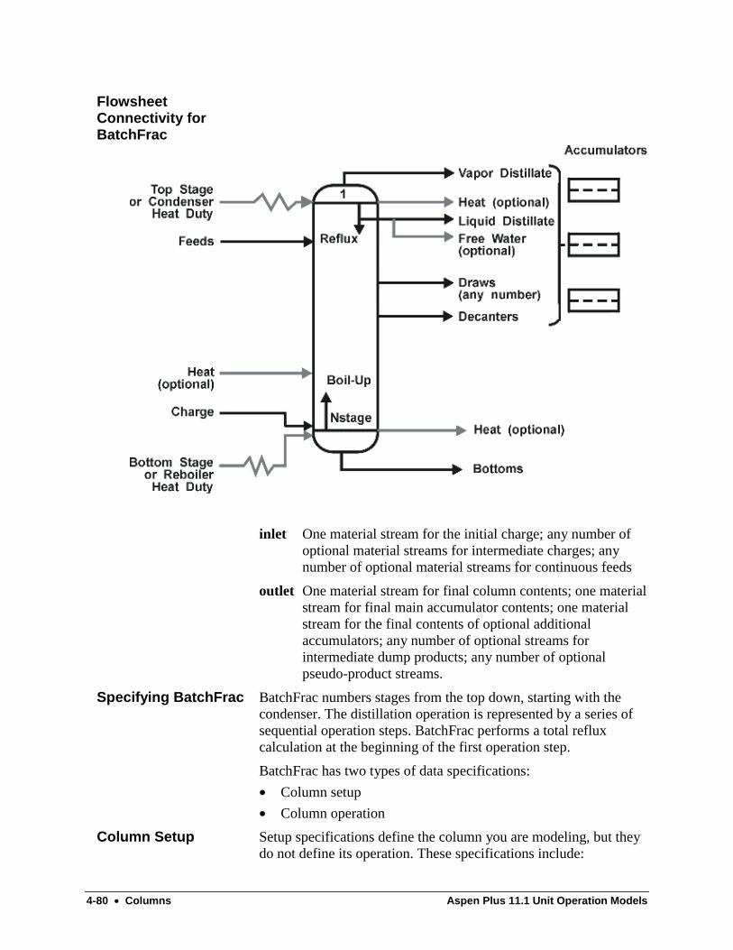
4-80 • Columns Aspen Plus 11.1 Unit Operation Models
inlet One material stream for the initial charge; any number ofoptional material streams for intermediate charges; anynumber of optional material streams for continuous feeds
outlet One material stream for final column contents; one materialstream for final main accumulator contents; one materialstream for the final contents of optional additionalaccumulators; any number of optional streams forintermediate dump products; any number of optionalpseudo-product streams.
BatchFrac numbers stages from the top down, starting with thecondenser. The distillation operation is represented by a series ofsequential operation steps. BatchFrac performs a total refluxcalculation at the beginning of the first operation step.
BatchFrac has two types of data specifications:
• Column setup
• Column operation
Setup specifications define the column you are modeling, but theydo not define its operation. These specifications include:
FlowsheetConnectivity forBatchFrac
Specifying BatchFrac
Column Setup
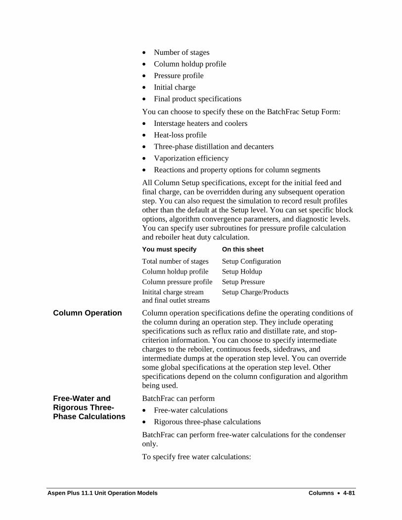
Aspen Plus 11.1 Unit Operation Models Columns • 4-81
• Number of stages
• Column holdup profile
• Pressure profile
• Initial charge
• Final product specifications
You can choose to specify these on the BatchFrac Setup Form:
• Interstage heaters and coolers
• Heat-loss profile
• Three-phase distillation and decanters
• Vaporization efficiency
• Reactions and property options for column segments
All Column Setup specifications, except for the initial feed andfinal charge, can be overridden during any subsequent operationstep. You can also request the simulation to record result profilesother than the default at the Setup level. You can set specific blockoptions, algorithm convergence parameters, and diagnostic levels.You can specify user subroutines for pressure profile calculationand reboiler heat duty calculation.
You must specify On this sheet
Total number of stages Setup Configuration
Column holdup profile Setup Holdup
Column pressure profile Setup Pressure
Initital charge streamand final outlet streams
Setup Charge/Products
Column operation specifications define the operating conditions ofthe column during an operation step. They include operatingspecifications such as reflux ratio and distillate rate, and stop-criterion information. You can choose to specify intermediatecharges to the reboiler, continuous feeds, sidedraws, andintermediate dumps at the operation step level. You can overridesome global specifications at the operation step level. Otherspecifications depend on the column configuration and algorithmbeing used.
BatchFrac can perform
• Free-water calculations
• Rigorous three-phase calculations
BatchFrac can perform free-water calculations for the condenseronly.
To specify free water calculations:
Column Operation
Free-Water andRigorous Three-Phase Calculations
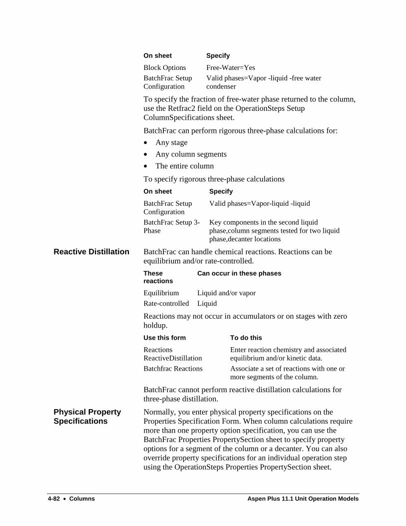
4-82 • Columns Aspen Plus 11.1 Unit Operation Models
On sheet Specify
Block Options Free-Water=Yes
BatchFrac SetupConfiguration
Valid phases=Vapor -liquid -free watercondenser
To specify the fraction of free-water phase returned to the column,use the Retfrac2 field on the OperationSteps SetupColumnSpecifications sheet.
BatchFrac can perform rigorous three-phase calculations for:
• Any stage
• Any column segments
• The entire column
To specify rigorous three-phase calculations
On sheet Specify
BatchFrac SetupConfiguration
Valid phases=Vapor-liquid -liquid
BatchFrac Setup 3-Phase
Key components in the second liquidphase,column segments tested for two liquidphase,decanter locations
BatchFrac can handle chemical reactions. Reactions can beequilibrium and/or rate-controlled.
Thesereactions
Can occur in these phases
Equilibrium Liquid and/or vapor
Rate-controlled Liquid
Reactions may not occur in accumulators or on stages with zeroholdup.
Use this form To do this
ReactionsReactiveDistillation
Enter reaction chemistry and associatedequilibrium and/or kinetic data.
Batchfrac Reactions Associate a set of reactions with one ormore segments of the column.
BatchFrac cannot perform reactive distillation calculations forthree-phase distillation.
Normally, you enter physical property specifications on theProperties Specification Form. When column calculations requiremore than one property option specification, you can use theBatchFrac Properties PropertySection sheet to specify propertyoptions for a segment of the column or a decanter. You can alsooverride property specifications for an individual operation stepusing the OperationSteps Properties PropertySection sheet.
Reactive Distillation
Physical PropertySpecifications

Aspen Plus 11.1 Unit Operation Models Columns • 4-83
When Feed-Convention=Above-Stage, a material stream isintroduced between adjacent stages. The liquid portion of thestream flows to the stage specified in the feed location Stage field.The vapor portion of the stream goes to the stage above (Stage 1).
You can introduce a By specifying
Liquid feed to the top stage (orcondenser
Stage=1
Vapor feed to the bottom stage (orreboiler)
Stage=Number Of Stages(Setup Configuration sheet) + 1
When Feed-Convention=On-Stage, both the liquid and vaporportions of a feed flow to the stage specified in the feed locationStage field.
Feed Conventions

4-84 • Columns Aspen Plus 11.1 Unit Operation Models
Extract ReferenceExtract is a rigorous model for simulating liquid-liquid extractors.It can have multiple feeds, heater/coolers, and side streams. Extractcan calculate distribution coefficients using:
• An activity coefficient model or equation of state capable ofrepresenting two liquid phases
• A built-in temperature-dependent correlation (KLL Correlationsheet)
• A Fortran subroutine (KLL Subroutine sheet)
Although equilibrium stages are assumed, you can specifycomponent or stage separation efficiencies. Extract can be usedonly for rating calculations.
You can define pseudoproduct streams (Report PseudoStreamssheet) to represent extractor internal flows. You can use Fortranand sensitivity blocks to vary configuration parameters, such asfeed location or number of stages.
Use the following forms to enter specifications and view results forExtract:
Use this form To do this
Setup Specify basic column configuration andoperating conditions
Efficiencies Specify stage or component efficiencies
Properties Specify parameters for KLL correlations andKLL subroutines
Estimates Specify initial estimates for stage temperaturesand compositions
Convergence Specify convergence parameters and block-specific diagnostic message levels
Report Specify block-specific report options andpseudostream information
Block Options Override global values for physical properties,simulation options, diagnostic message levels,and report options for this block
Results View column performance summary, materialand energy balance results, and split fractions
Profiles View extractor profiles
Dynamic Specify parameters for dynamic simulations

Aspen Plus 11.1 Unit Operation Models Columns • 4-85
L1 Phase
L1 Phase
L2 Phase
Side products(any number)(any number)
Side feeds
L2 Phase
Nstage
1
Material Streams
inlet One material stream to the first (top) stage, rich in the firstliquid phase (L1)One material stream to the last (bottom) stage, rich in thesecond liquid phase (L2)One material stream per intermediate stage (optional)
outlet One material stream for L1 from the last stageOne material stream for L2 from the first stageUp to two side product streams per stage, one for L1 andone for L2 (optional)
Extract can operate in one of the following ways:
• Adiabatically (default)
• At a specified temperature
• With specified stage heater or cooler duties
You must specify:
• Number of stages
• Feed and product stream stage locations
• Side product stream phase and mole flow rate
• Pressure profile
The first liquid phase (L1) flows from the first stage to the laststage. The second (L2) flows in the opposite direction. You mustidentify the key components in each phase using L1-Comps andL2-Comps on the Setup form. Extract can treat phase L1 as thesolvent/extract phase or the feed/raffinate phase.
FlowsheetConnectivity forExtract
Specifying Extract
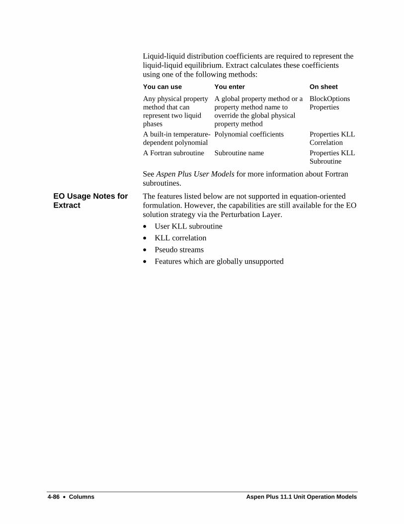
4-86 • Columns Aspen Plus 11.1 Unit Operation Models
Liquid-liquid distribution coefficients are required to represent theliquid-liquid equilibrium. Extract calculates these coefficientsusing one of the following methods:
You can use You enter On sheet
Any physical propertymethod that canrepresent two liquidphases
A global property method or aproperty method name tooverride the global physicalproperty method
BlockOptionsProperties
A built-in temperature-dependent polynomial
Polynomial coefficients Properties KLLCorrelation
A Fortran subroutine Subroutine name Properties KLLSubroutine
See Aspen Plus User Models for more information about Fortransubroutines.
The features listed below are not supported in equation-orientedformulation. However, the capabilities are still available for the EOsolution strategy via the Perturbation Layer.
• User KLL subroutine
• KLL correlation
• Pseudo streams
• Features which are globally unsupported
EO Usage Notes forExtract
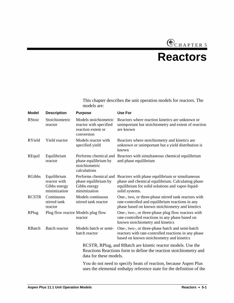
Aspen Plus 11.1 Unit Operation Models Reactors • 5-1
C H A P T E R 5
Reactors
This chapter describes the unit operation models for reactors. Themodels are:
Model Description Purpose Use For
RStoic Stoichiometricreactor
Models stoichiometricreactor with specifiedreaction extent orconversion
Reactors where reaction kinetics are unknown orunimportant but stoichiometry and extent of reactionare known
RYield Yield reactor Models reactor withspecified yield
Reactors where stoichiometry and kinetics areunknown or unimportant but a yield distribution isknown
REquil Equilibriumreactor
Performs chemical andphase equilibrium bystoichiometriccalculations
Reactors with simultaneous chemical equilibriumand phase equilibrium
RGibbs Equilibriumreactor withGibbs energyminimization
Performs chemical andphase equilibrium byGibbs energyminimization
Reactors with phase equilibrium or simultaneousphase and chemical equilibrium. Calculating phaseequilibrium for solid solutions and vapor-liquid-solid systems.
RCSTR Continuousstirred tankreactor
Models continuousstirred tank reactor
One-, two, or three-phase stirred tank reactors withrate-controlled and equilibrium reactions in anyphase based on known stoichiometry and kinetics
RPlug Plug flow reactor Models plug flowreactor
One-, two-, or three-phase plug flow reactors withrate-controlled reactions in any phase based onknown stoichiometry and kinetics
RBatch Batch reactor Models batch or semi-batch reactor
One-, two-, or three-phase batch and semi-batchreactors with rate-controlled reactions in any phasebased on known stoichiometry and kinetics
RCSTR, RPlug, and RBatch are kinetic reactor models. Use theReactions Reactions form to define the reaction stoichiometry anddata for these models.
You do not need to specify heats of reaction, because Aspen Plususes the elemental enthalpy reference state for the definition of the

5-2 • Reactors Aspen Plus 11.1 Unit Operation Models
component heat of formation. Therefore, heats of reaction areaccounted for in the mixture enthalpy calculations for the reactantsversus the products.

Aspen Plus 11.1 Unit Operation Models Reactors • 5-3
RStoic ReferenceUse RStoic to model a reactor when:
• Reaction kinetics are unknown or unimportant and
• Stoichiometry and the molar extent or conversion is known foreach reaction
RStoic can model reactions occurring simultaneously orsequentially. In addition, RStoic can perform product selectivityand heat of reaction calculations.
Use the following forms to enter specifications and view results forRStoic:
Use this form To do this
Setup Specify operating conditions, reactions, referenceconditions for heat of reaction calculations, productand reactant components for selectivity calculations,particle size distribution, and component attributes
Convergence Specify estimates and convergence parameters forflash calculations
BlockOptions Override global values for physical properties,simulation options, diagnostic message levels, andreport options for this block
Results View summary of operating results, mass andenergy balances, heats of reaction, productselectivities, reaction extents, and phase equilibriumresults for the outlet stream
Dynamic Specify parameters for dynamic simulations
Material
Water (optional)
Heat (optional)
Material(any number)
Heat(optional)
Material Streams
inlet At least one material stream
outlet One product streamOne water decant stream (optional)
FlowsheetConnectivity forRStoic
5-4 • Reactors Aspen Plus 11.1 Unit Operation Models
Heat Stream
inlet Any number of heat streams (optional)
RStoic uses the sum of the inlet heat streams as the heat dutyspecification, if you do not specify an outlet heat stream.
outlet One heat stream (optional)
The value of the outlet heat stream is the net heat duty (sum of theinlet heat streams minus the calculated heat duty) for the reactor.
Use the Setup Specifications sheet to specify the reactor operatingconditions and to select the phases to consider in flash calculationsin the reactor.
Use the Setup Reactions sheet to define the reactions occurring inthe reactor. You must specify the stoichiometry for each reaction.In addition, you must specify either the molar extent or thefractional conversion for all reactions. Alternatively, you can usethe Setup Combustion sheet to have RStoic generate combustionreactions.
When solids are created or changed by the reactions, you mayspecify the component attributes and the particle size distributionin the outlet stream using the Setup Component Attr. sheet and theSetup PSD sheet respectively.
If you wish to calculate the heats of reaction, use the Setup Heat ofReaction sheet to specify the reference component for eachreaction defined in the Setup Reactions sheet. You may alsochoose to specify the heats of reaction, and RStoic adjusts thecalculated reactor duty, if needed.
If you wish to calculate product selectivities use the SetupSelectivity sheet to specify the selected product component and thereference reactant component.
RStoic calculates the heat of reaction from the heats of formationin the databanks when you select the Calculate Heat of Reactionoption on the Setup Heat of Reaction sheet. The heats of reactionare calculated at the specified reference conditions based onconsumption of a unit mole or mass of the reference reactantselected for each reaction. The following reference conditions areused by default:
Specification Default
Reference temperature 25 degrees C
Reference pressure 1 atm
Reference fluid phase Vapor phase
You can also use the Setup Heat of Reaction sheet to specify theheats of reaction. The specified heat of reaction may differ from
Specifying RStoic
Heat of Reaction
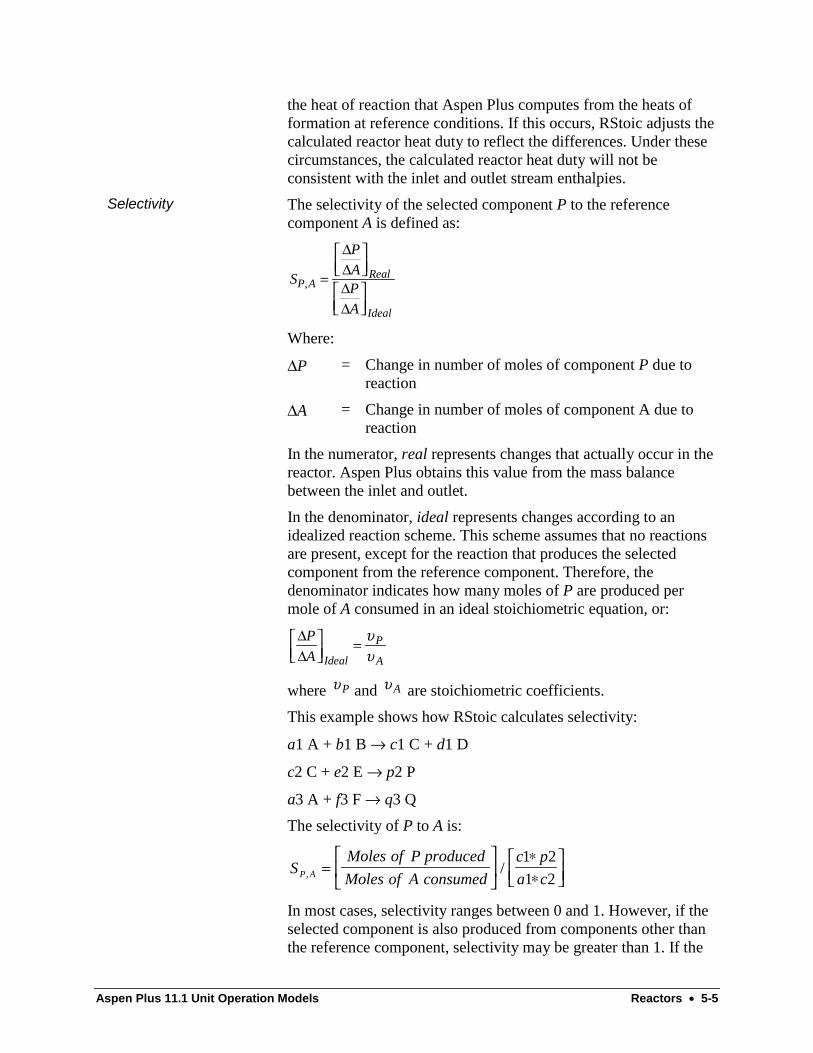
Aspen Plus 11.1 Unit Operation Models Reactors • 5-5
the heat of reaction that Aspen Plus computes from the heats offormation at reference conditions. If this occurs, RStoic adjusts thecalculated reactor heat duty to reflect the differences. Under thesecircumstances, the calculated reactor heat duty will not beconsistent with the inlet and outlet stream enthalpies.
The selectivity of the selected component P to the referencecomponent A is defined as:
S
P
AP
A
P A, =
∆∆∆∆
Real
Ideal
Where:
∆P = Change in number of moles of component P due toreaction
∆A = Change in number of moles of component A due toreaction
In the numerator, real represents changes that actually occur in thereactor. Aspen Plus obtains this value from the mass balancebetween the inlet and outlet.
In the denominator, ideal represents changes according to anidealized reaction scheme. This scheme assumes that no reactionsare present, except for the reaction that produces the selectedcomponent from the reference component. Therefore, thedenominator indicates how many moles of P are produced permole of A consumed in an ideal stoichiometric equation, or:
∆∆
P
A Ideal
P
A
= υυ
where υP and υ A are stoichiometric coefficients.
This example shows how RStoic calculates selectivity:
a1 A + b1 B → c1 C + d1 D
c2 C + e2 E → p2 P
a3 A + f3 F → q3 Q
The selectivity of P to A is:
SMoles of P produced
Moles of A consumed
c p
a cP A, /=
∗∗
1 2
1 2
In most cases, selectivity ranges between 0 and 1. However, if theselected component is also produced from components other thanthe reference component, selectivity may be greater than 1. If the
Selectivity

5-6 • Reactors Aspen Plus 11.1 Unit Operation Models
selected component is consumed in other reactions, selectivity maybe less than 0.
The features listed below are not supported in equation-orientedformulation. However, the capabilities are still available for the EOsolution strategy via the Perturbation Layer.
• Reactions in series
• Specifications which result in modified conversions duringsequential-modular calculations
• Features which are globally unsupported
EO Usage Notes forRStoic

Aspen Plus 11.1 Unit Operation Models Reactors • 5-7
RYield ReferenceUse RYield to model a reactor when:
• Reaction stoichiometry is unknown or unimportant
• Reaction kinetics are unknown or unimportant
• Yield distribution is known
You must specify the yields (per mass of total feed, excluding anyinert components) for the products or calculate them in a user-supplied Fortran subroutine. RYield normalizes the yields tomaintain a mass balance. RYield can model one-, two-, and three-phase reactors.
Use the following forms to enter specifications and view results forRYield:
Use this form To do this
Setup Specify reactor operating conditions, componentyields, inert components, flash convergenceparameters, and PSD and component attributes forthe outlet stream
Assay Analysis Specify distillation, gravity, molecular weight,petroleum properties, and viscosity data forpetroleum characterization and petroleum propertiescalculation
UserSubroutine Specify subroutine name and parameters for theuser-supplied yield subroutine
Dynamic Specify parameters for dynamic simulations
BlockOptions Override global values for physical properties,simulation options, diagnostic message levels, andreport options for this block
Results View summary of operating results, mass andenergy balances for the reactor and phaseequilibrium results for the outlet stream
Material
Water (optional)
Heat (optional)
Material(any number)
Heat(optional)
FlowsheetConnectivity forRYield

5-8 • Reactors Aspen Plus 11.1 Unit Operation Models
Material Streams
inlet At least one material stream
outlet One product streamOne water decant stream (optional)
Heat Streams
inlet Any number of heat streams (optional)
outlet One heat stream (optional)
If you give only one specification on the Setup Specifications sheet(temperature or pressure), RYield uses the sum of the inlet heatstreams as a duty specification. Otherwise, RYield uses the inletheat stream(s) only to calculate the net heat duty. The net heat dutyis the sum of the inlet heat streams minus the actual (calculated)heat duty.
You can use an outlet heat stream for the net heat duty.
Use the Setup Specifications and Setup Yield sheets to specify thereactor conditions and the component yields. For each reactionproduct, specify the yield as either moles or mass of a componentper unit mass of feed. If you specify inert components on the SetupYield sheet, the yields will be based on unit mass of non-inert feed.
Calculated yields are normalized to maintain an overall materialbalance. For this reason, yield specifications establish a yielddistribution, rather than absolute yields. RYield does not maintainatom balances because you enter the fixed yield distribution.
You can also use Ryield to re-characterize an assay or a blenddefined on the Components Assay/Blend Form.
You can request one-, two-, or three-phase calculation.
When solids are created or changed by the reactions, you canspecify their component attributes and/or particle size distributionin the outlet stream using the Setup Component Attr. and SetupPSD sheets, respectively.
The features listed below are not supported in equation-orientedformulation. However, the capabilities are still available for the EOsolution strategy via the Perturbation Layer.
• User yield subroutines
• Specifications which result in renormalized yields duringsequential-modular calculations
• Petroleum characterization option for specifying yield
• Features which are globally unsupported
Specifying RYield
EO Usage Notes forRYield
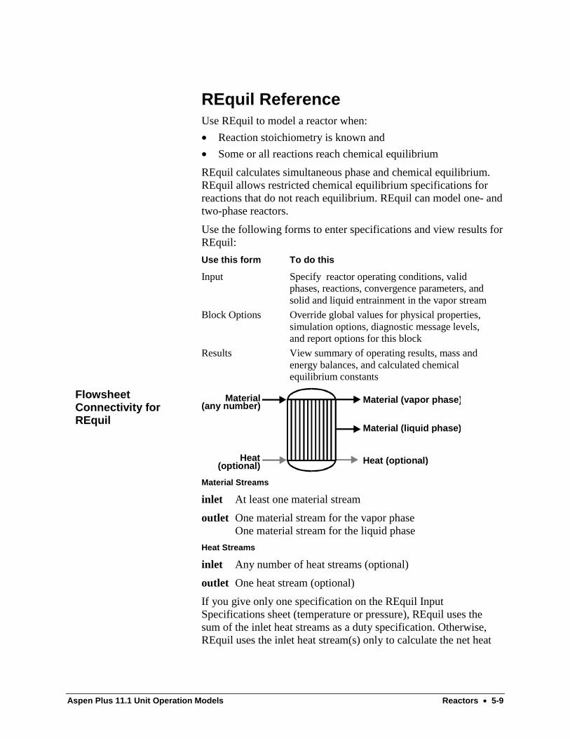
Aspen Plus 11.1 Unit Operation Models Reactors • 5-9
REquil ReferenceUse REquil to model a reactor when:
• Reaction stoichiometry is known and
• Some or all reactions reach chemical equilibrium
REquil calculates simultaneous phase and chemical equilibrium.REquil allows restricted chemical equilibrium specifications forreactions that do not reach equilibrium. REquil can model one- andtwo-phase reactors.
Use the following forms to enter specifications and view results forREquil:
Use this form To do this
Input Specify reactor operating conditions, validphases, reactions, convergence parameters, andsolid and liquid entrainment in the vapor stream
Block Options Override global values for physical properties,simulation options, diagnostic message levels,and report options for this block
Results View summary of operating results, mass andenergy balances, and calculated chemicalequilibrium constants
Heat (optional)
Material (vapor phase)
Material (liquid phase)
Material(any number)
Heat(optional)
Material Streams
inlet At least one material stream
outlet One material stream for the vapor phaseOne material stream for the liquid phase
Heat Streams
inlet Any number of heat streams (optional)
outlet One heat stream (optional)
If you give only one specification on the REquil InputSpecifications sheet (temperature or pressure), REquil uses thesum of the inlet heat streams as a duty specification. Otherwise,REquil uses the inlet heat stream(s) only to calculate the net heat
FlowsheetConnectivity forREquil

5-10 • Reactors Aspen Plus 11.1 Unit Operation Models
duty. The net heat duty is the sum of the inlet heat streams minusthe actual (calculated) heat duty.
You can use an outlet heat stream for the net heat duty.
You must specify the reaction stoichiometry and the reactorconditions. If no additional specifications are given, REquilassumes that the reactions will reach equilibrium.
REquil calculates equilibrium constants from the Gibbs energy.You can restrict the equilibrium by specifying one of thefollowing:
• The molar extent for any reaction
• A temperature approach to chemical equilibrium (for anyreaction)
If you specify temperature approach, ∆T, REquil evaluates thechemical equilibrium constant at T + ∆T, where T is the reactortemperature (specified or calculated).
REquil performs single-phase property calculations or two-phaseflash calculations nested inside a chemical equilibrium loop.REquil cannot perform three-phase calculations.
Reactions can include conventional solids. REquil treats eachparticipating solid component as a separate pure solid phase, not asa component in a solid solution. Any participating solids must havea free energy formation (DGSFRM) and enthalpy of formation(DHSFRM), or heat capacity parameters (CPSXP1).
Solids not participating in reactions, including anynonconventional components, are treated as inert. These solidshave no effect on the equilibrium calculations except on the energybalance.
Specifying REquil
Solids
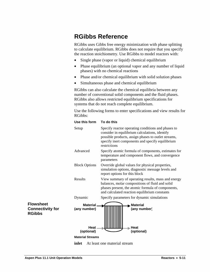
Aspen Plus 11.1 Unit Operation Models Reactors • 5-11
RGibbs ReferenceRGibbs uses Gibbs free energy minimization with phase splittingto calculate equilibrium. RGibbs does not require that you specifythe reaction stoichiometry. Use RGibbs to model reactors with:
• Single phase (vapor or liquid) chemical equilibrium
• Phase equilibrium (an optional vapor and any number of liquidphases) with no chemical reactions
• Phase and/or chemical equilibrium with solid solution phases
• Simultaneous phase and chemical equilibrium
RGibbs can also calculate the chemical equilibria between anynumber of conventional solid components and the fluid phases.RGibbs also allows restricted equilibrium specifications forsystems that do not reach complete equilibrium.
Use the following forms to enter specifications and view results forRGibbs:
Use this form To do this
Setup Specify reactor operating conditions and phases toconsider in equilibrium calculations, identifypossible products, assign phases to outlet streams,specify inert components and specify equilibriumrestrictions
Advanced Specify atomic formula of components, estimates fortemperature and component flows, and convergenceparameters
Block Options Override global values for physical properties,simulation options, diagnostic message levels andreport options for this block
Results View summary of operating results, mass and energybalances, molar compositions of fluid and solidphases present, the atomic formula of components,and calculated reaction equilibrium constants
Dynamic Specify parameters for dynamic simulations
Material(any number)
Material(any number)
Heat(optional)
Heat(optional)
Material Streams
inlet At least one material stream
FlowsheetConnectivity forRGibbs
5-12 • Reactors Aspen Plus 11.1 Unit Operation Models
outlet At least one material stream
If you specify as many outlet streams as the number of phases thatRGibbs calculates, RGibbs assigns each phase to an outlet stream.If you specify fewer outlet streams, RGibbs assigns the additionalphases to the last outlet stream.
Heat Streams
inlet Any number of heat streams (optional)
outlet One heat stream (optional)
If you specify only pressure on the Setup Specifications sheet,RGibbs uses the sum of the inlet heat streams as a dutyspecification. Otherwise, RGibbs uses the inlet heat stream(s) onlyto calculate the net heat duty. The net heat duty is the sum of theinlet heat streams minus the actual (calculated) heat duty.
You can use an outlet heat stream for the net heat duty.
This section describes how to specify:
• Phase equilibrium only
• Phase and chemical equilibrium
• Restricted chemical equilibrium
• Reactions
• Solids
To specify Use this option On
Phase equilibrium calculationsonly
Phase Equilibrium Only Setup Specifications sheet
Maximum number of fluidphases that RGibbs shouldconsider
Maximum Number of FluidPhases
Setup Specifications sheet
Maximum number of solidsolution phases
Maximum Number of SolidSolution Phases
Solid Phases dialog box from the SetupSpecifications sheet
RGibbs distributes all species among all solution phases by default.You can use the Setup Products sheet to assign different sets ofspecies to each solution phase. You can also assign differentthermodynamic property methods to each phase.
If there is a possibility that a solid solution phase may exist, use theSetup Products sheet to identify the species that will exist in thatphase.
Specifying RGibbs
Phase Equilibrium Only
Aspen Plus 11.1 Unit Operation Models Reactors • 5-13
To specify Use this option On
Chemical equilibriumcalculations (with or withoutphase equilibrium)
Phase Equilibrium andChemical Equilibrium
Setup Specifications sheet
Maximum number of fluidphases that RGibbs shouldconsider
Maximum Number of FluidPhases
Setup Specifications sheet
Maximum number of solidsolution phases
Maximum Number of SolidSolution Phases
Solid Phases dialog box from the SetupSpecifications sheet
By default, RGibbs considers all components entered on theComponents Specifications Selection sheet as possible fluid phaseor solid products. You can specify an alternate list of products onthe Setup Products sheet.
RGibbs distributes all solution species among all solution phasesby default. You can use the Setup Products sheet to assign differentsets of species to each solution phase. You can also assign differentthermodynamic property methods to each phase.
RGibbs needs the molecular formula for each component that ispresent in a feed or product stream. RGibbs retrieves thisinformation from the component databanks. For non-databankcomponents, use the Properties Molec-Struct Formula sheet toenter:
• Atom (the atom type)
• Number of occurrences (the number of atoms of each type)
Alternatively, you can enter the atom matrix on the AdvancedAtom Matrix sheet. The atom matrix defines the number of eachatom in each component. If you enter the atom matrix, you mustenter it for all components and atoms, including databankcomponents.
If there is a possibility that a solid solution phase may exist, use theSetup Products sheet to identify the species which will exist in thatphase.
Phase Equilibrium andChemical Equilibrium

5-14 • Reactors Aspen Plus 11.1 Unit Operation Models
To restrict chemical equilibrium:
Specify On
The molar extent of the reaction Edit Reactions dialog box (from theSetup RestrictedEquilibrium sheet)
A temperature approach toequilibrium for individualreactions
Edit Reactions dialog box (from theSetup RestrictedEquilibrium sheet)
A temperature approach tochemical equilibrium for theentire system
Edit Reactions dialog box (from theSetup RestrictedEquilibrium sheet)
The outlet amount of anycomponent as total mole flow oras a fraction of the feed of thatcomponent
Setup Inerts sheet †
† You can specify inert components by setting the fraction to 1.
For temperature approach specifications, RGibbs evaluates thechemical equilibrium constant at T + ∆T, where T is the actualreactor temperature (specified or calculated) and ∆T is the desiredtemperature approach.
You can enter one of the following restricted equilibriumspecifications for individual reactions:
• The molar extent of a reaction
• The temperature approach for an individual reaction
Use the Setup RestrictedEquilibrium sheet to supply the reactionstoichiometry.
If you enter one of the preceding specifications, you must alsosupply the stoichiometry for a set of linearly independent reactionsinvolving all components in the system.
You can have RGibbs consider only a specific set of reactions.You can restrict the chemical equilibrium by specifyingtemperature approach or molar extent for the reactions. You mustspecify the stoichiometric coefficients for a complete set oflinearly independent chemical reactions, even if only one reactionis restricted.
The number of linearly independent reactions required equals thetotal number of products in the product list, including solids (seethe Setup Products sheet), minus the number of atoms present inthe system. The reactions must involve all participatingcomponents. A component is participating if it satisfies thesecriteria:
• It is in the product list.
Restricted ChemicalEquilibrium
Reactions

Aspen Plus 11.1 Unit Operation Models Reactors • 5-15
• It is not inert. A component is inert if it consists entirely ofatoms not present in any other product components.
• It has not been dropped. A component listed on the SetupProducts sheet is dropped if it contains an atom not present inthe feed.
RGibbs can calculate the chemical equilibria between any numberof conventional solid components and the fluid phases. RGibbsdetects whether the solid is present at equilibrium, and if so,calculates the amount. RGibbs treats each solid component as apure solid phase, unless it is specified as a component in a solidsolution. Any solid that RGibbs considers a product must haveboth:
• Free energy of formation (DGSFRM or CPSXP1)
• Heat of formation (DHSFRM or CPSXP1)
Nonconventional solids are treated as inert and have no effect onequilibrium calculations. If chemical equilibrium is not considered,RGibbs treats all solids as inert. RGibbs cannot perform solids-phase-only calculations.
RGibbs places all pure solids in the last outlet stream unless youspecify otherwise on the Setup AssignStreams sheet. RGibbs canhandle only a single CISOLID substream, which contains allconventional solids products defined as pure solid phases. RGibbsplaces the solid solution phases in the MIXED substream of theoutlet stream(s).
RGibbs cannot directly handle phase equilibrium between solidsand fluid phases (for example, water-ice equilibrium). To workaround this, you can list the same component twice on theComponents Specifications Selection sheet, with differentcomponent IDs. If you want RGibbs to calculate the chemicalequilibrium between these components:
• Specify both component IDs on the Setup Products sheet.
• Designate one ID as a solids phase component, the other as afluid phase component.
Gautam, R. and Seider, W.D., "Computation of Phase andChemical Equilibrium," Parts I, II, and III, AIChE J. 25, 6,November, 1979, pp. 991-1015.
White, C.W. and Seider, W.D., "Computation of Phase andChemical Equilibrium: Approach to Chemical Equilibrium,"AIChE J., 27, 3, May, 1981, pp.446-471.
Schott, G. L., "Computation of Restricted Equilibria by GeneralMethods," J. Chem. Phys., 40, 1964.
Solids
References

5-16 • Reactors Aspen Plus 11.1 Unit Operation Models
RCSTR ReferenceRCSTR rigorously models continuous stirred tank reactors.RCSTR can model one-, two-, or three-phase reactors. RCSTRassumes perfect mixing in the reactor, that is, the reactor contentshave the same properties and composition as the outlet stream.
RCSTR handles kinetic and equilibrium reactions as well asreactions involving solids. You can provide the reaction kineticsthrough the built-in Reactions models or through a user-definedFortran subroutine.
Use the following forms to enter specifications and view results forRCSTR:
Use this form To do this
Setup Specify reactor operating conditions and holdup,select the reaction sets to be included, andspecify PSD and component attributes in theoutlet stream
Convergence Provide estimates for component flow rates,reactor temperature and volume, and specifyflash convergence parameters, RCSTRconvergence methods and parameters, andinitialization options
UserSubroutine Specify parameters for the user-supplied kineticssubroutine and block-specific report option forthe kinetics subroutine
BlockOptions Override global values for physical properties,simulation options, diagnostic message levels,and report options for this block
Results View summary of operating results and mass andenergy balances for the block
Dynamic Specify parameters for dynamic simulations
Material
Heat (optional)
Material(any number)
Heat(optional)
FlowsheetConnectivity forRCSTR

Aspen Plus 11.1 Unit Operation Models Reactors • 5-17
Material Streams
inlet At least one material stream
outlet One material stream
Heat Streams
inlet Any number of heat streams (optional)
outlet One heat stream (optional)
If you specify only pressure on the Setup Specifications sheet,RCSTR uses the sum of the inlet heat streams as a dutyspecification. Otherwise, RCSTR uses the inlet heat stream only tocalculate the net heat duty. The net heat duty is the sum of the inletheat streams minus the actual (calculated) heat duty.
You can use an outlet heat stream for the net heat duty.
You must specify the reactor operating conditions, which arepressure and either temperature or heat duty. You must also enterthe reactor volume or residence time (overall or phase).
You must specify reaction kinetics on the Reactions Reactionsforms and select the Reaction Set ID on the Setup Reactions sheet.
You can specify one-, two-, or three-phase calculations. You canspecify the phase for each reaction on the Reactions Reactionsforms. RCSTR can handle the kinetic and equilibrium typereactions.
In a multi-phase reactor, by default, Aspen Plus calculates thevolume of each phase, using phase equilibrium results, as:
V VV f
V fPi Ri i
j j
=Σ
Where:
VPi = Volume of phase i
VR = Reactor volume
Vi = Molar volume of phase i
f i = Molar fraction of phase i
You can override the default calculation by specifying the volumeof a phase directly (Phase Volume) or as a fraction of the reactorvolume (Phase Volume Frac) on the Setup Specifications sheet.
Alternatively, when you specify the residence time of a phase inthe reactor, Aspen Plus calculates the phase volume iteratively.
Specifying RCSTR
Reactions
Phase Volume
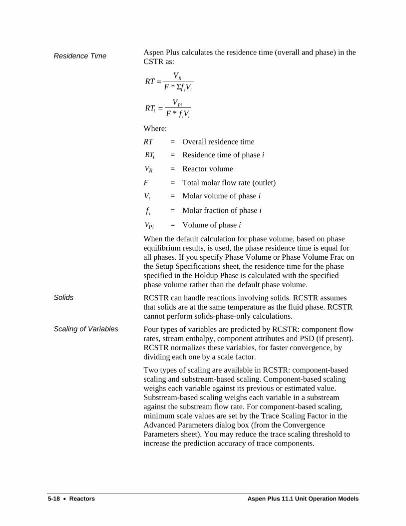
5-18 • Reactors Aspen Plus 11.1 Unit Operation Models
Aspen Plus calculates the residence time (overall and phase) in theCSTR as:
RTV
F f VR
i i
=*Σ
RTV
F f ViPi
i i
=*
Where:
RT = Overall residence time
RTi = Residence time of phase i
VR = Reactor volume
F = Total molar flow rate (outlet)
Vi = Molar volume of phase i
f i = Molar fraction of phase i
VPi = Volume of phase i
When the default calculation for phase volume, based on phaseequilibrium results, is used, the phase residence time is equal forall phases. If you specify Phase Volume or Phase Volume Frac onthe Setup Specifications sheet, the residence time for the phasespecified in the Holdup Phase is calculated with the specifiedphase volume rather than the default phase volume.
RCSTR can handle reactions involving solids. RCSTR assumesthat solids are at the same temperature as the fluid phase. RCSTRcannot perform solids-phase-only calculations.
Four types of variables are predicted by RCSTR: component flowrates, stream enthalpy, component attributes and PSD (if present).RCSTR normalizes these variables, for faster convergence, bydividing each one by a scale factor.
Two types of scaling are available in RCSTR: component-basedscaling and substream-based scaling. Component-based scalingweighs each variable against its previous or estimated value.Substream-based scaling weighs each variable in a substreamagainst the substream flow rate. For component-based scaling,minimum scale values are set by the Trace Scaling Factor in theAdvanced Parameters dialog box (from the ConvergenceParameters sheet). You may reduce the trace scaling threshold toincrease the prediction accuracy of trace components.
Residence Time
Solids
Scaling of Variables

Aspen Plus 11.1 Unit Operation Models Reactors • 5-19
Component-based scaling generally provides more accuracy thansubstream-based scaling, especially for trace components. Usecomponent-based scaling when:
• The reaction network involves trace intermediates
• The reaction rates are very sensitive to trace reactants (such ascatalysts and initiators which participate in degradationreactions)
The following tables summarize the scale factors used by eachmethod.
Substream-based Scaling Method
Variable Type Variable Initial Scale Factor
Component Flows Component mole flow in outlet stream Estimated outlet substream mole flowrate
Stream Enthalpy Net enthalpy flow of outlet stream Net enthalpy flow of inlet stream
ComponentAttributes (attr/kg)
Product of component mass flow (withattributes) and attribute value in outlet stream
Default attribute scale factor
PSD Product of substream mass flow rate (withPSD) and PSD value in outlet stream
Default attribute scale factor
Note: If any substream-based scaling factor is equal to zero, thedefault scaling factor is used instead (the default factor is 1.0 forcomponent flow rates and 1.0E5 for stream enthalpy).
Component-based Scaling Method
Variable Type Variable Initial Scale Factor
Component Flows Component mole flow in outletstream
Larger of:
- Estimated component mole flow in outletstream
- Product of Trace threshold and estimatedoutlet substream mole flow
Stream Enthalpy Net enthalpy flow of outlet stream Net enthalpy flow of inlet stream
ComponentAttributes (attr/kg)
Product of component mass flowwith attributes and attribute value inoutlet stream
Larger of:
- Product of estimated attributed componentmass flow and estimated attribute value in outletstream
- Product of Trace threshold and estimatedoutlet substream mole flow
PSD Product of substream mass flow rateand PSD value in outlet stream
Larger of:
- Product of estimated substream mass flow withPSDs and estimated PSD value in outlet stream
- Product of Trace threshold and defaultattribute scale factor
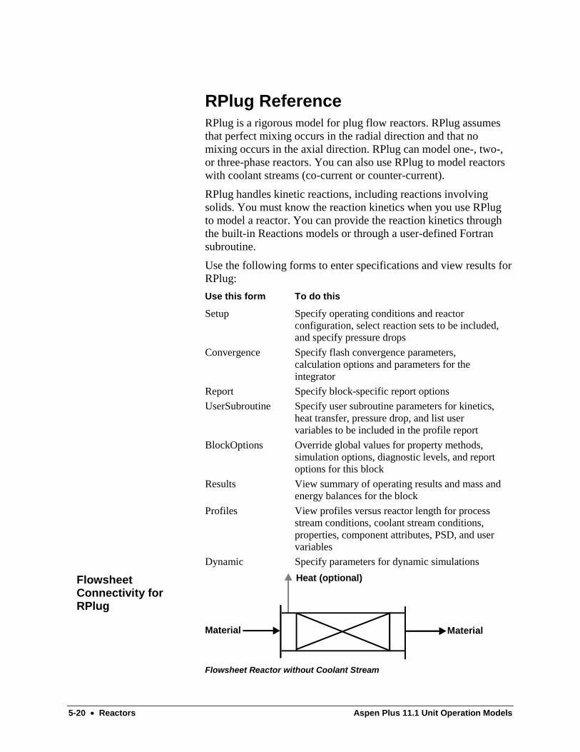
5-20 • Reactors Aspen Plus 11.1 Unit Operation Models
RPlug ReferenceRPlug is a rigorous model for plug flow reactors. RPlug assumesthat perfect mixing occurs in the radial direction and that nomixing occurs in the axial direction. RPlug can model one-, two-,or three-phase reactors. You can also use RPlug to model reactorswith coolant streams (co-current or counter-current).
RPlug handles kinetic reactions, including reactions involvingsolids. You must know the reaction kinetics when you use RPlugto model a reactor. You can provide the reaction kinetics throughthe built-in Reactions models or through a user-defined Fortransubroutine.
Use the following forms to enter specifications and view results forRPlug:
Use this form To do this
Setup Specify operating conditions and reactorconfiguration, select reaction sets to be included,and specify pressure drops
Convergence Specify flash convergence parameters,calculation options and parameters for theintegrator
Report Specify block-specific report options
UserSubroutine Specify user subroutine parameters for kinetics,heat transfer, pressure drop, and list uservariables to be included in the profile report
BlockOptions Override global values for property methods,simulation options, diagnostic levels, and reportoptions for this block
Results View summary of operating results and mass andenergy balances for the block
Profiles View profiles versus reactor length for processstream conditions, coolant stream conditions,properties, component attributes, PSD, and uservariables
Dynamic Specify parameters for dynamic simulations
Material Material
Heat (optional)
Flowsheet Reactor without Coolant Stream
FlowsheetConnectivity forRPlug

Aspen Plus 11.1 Unit Operation Models Reactors • 5-21
Material Material
Material Coolant(optional)
Material Coolant(optional)
Flowsheet Reactor with Coolant Stream
Material Streams
inlet One material feed streamOne coolant stream (optional)
outlet One material product streamOne coolant stream (optional)
Heat Streams
inlet No inlet heat streams
outlet One heat stream (optional) for the reactor heat duty. Usethe heat outlet stream only for reactors without a coolantstream.
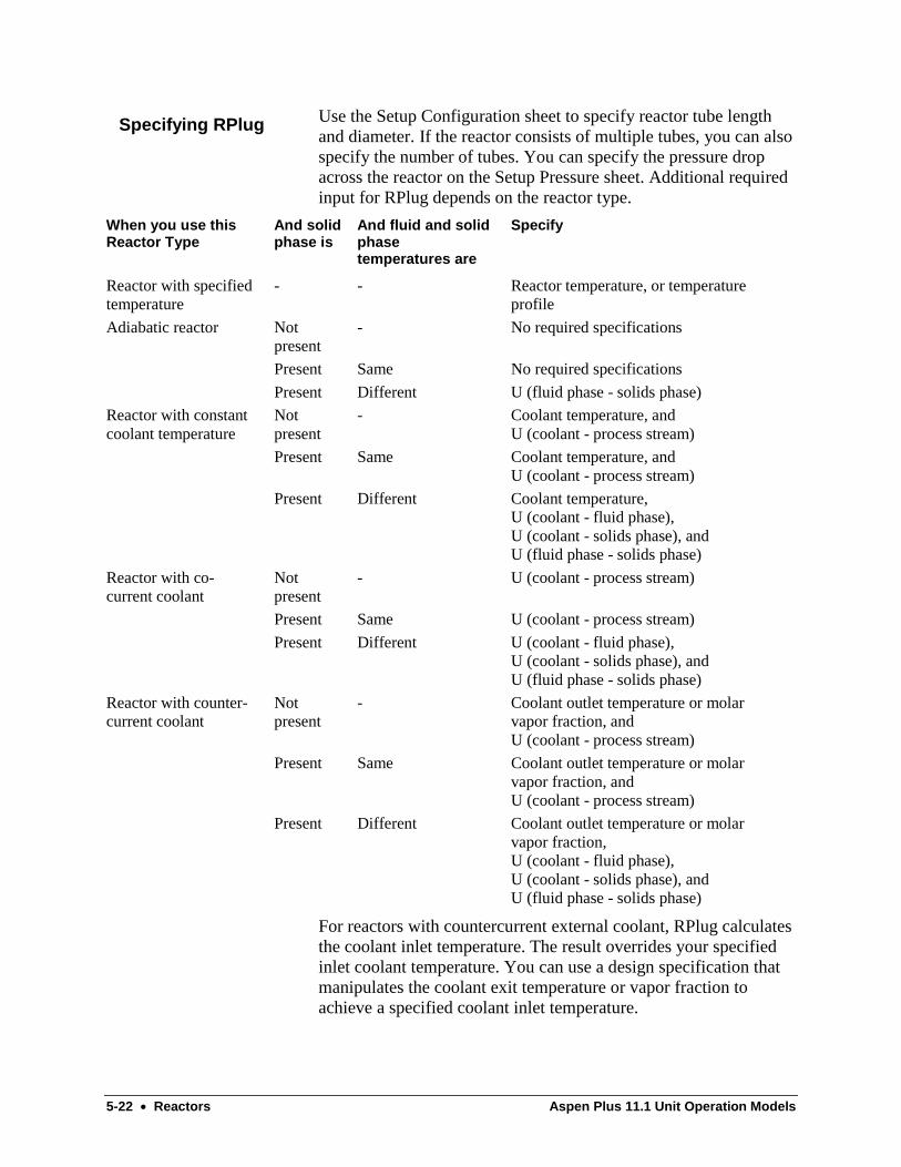
5-22 • Reactors Aspen Plus 11.1 Unit Operation Models
Use the Setup Configuration sheet to specify reactor tube lengthand diameter. If the reactor consists of multiple tubes, you can alsospecify the number of tubes. You can specify the pressure dropacross the reactor on the Setup Pressure sheet. Additional requiredinput for RPlug depends on the reactor type.
When you use thisReactor Type
And solidphase is
And fluid and solidphasetemperatures are
Specify
Reactor with specifiedtemperature
- - Reactor temperature, or temperatureprofile
Adiabatic reactor Notpresent
- No required specifications
Present Same No required specifications
Present Different U (fluid phase - solids phase)
Reactor with constantcoolant temperature
Notpresent
- Coolant temperature, andU (coolant - process stream)
Present Same Coolant temperature, andU (coolant - process stream)
Present Different Coolant temperature,U (coolant - fluid phase),U (coolant - solids phase), andU (fluid phase - solids phase)
Reactor with co-current coolant
Notpresent
- U (coolant - process stream)
Present Same U (coolant - process stream)
Present Different U (coolant - fluid phase),U (coolant - solids phase), andU (fluid phase - solids phase)
Reactor with counter-current coolant
Notpresent
- Coolant outlet temperature or molarvapor fraction, andU (coolant - process stream)
Present Same Coolant outlet temperature or molarvapor fraction, andU (coolant - process stream)
Present Different Coolant outlet temperature or molarvapor fraction,U (coolant - fluid phase),U (coolant - solids phase), andU (fluid phase - solids phase)
For reactors with countercurrent external coolant, RPlug calculatesthe coolant inlet temperature. The result overrides your specifiedinlet coolant temperature. You can use a design specification thatmanipulates the coolant exit temperature or vapor fraction toachieve a specified coolant inlet temperature.
Specifying RPlug

Aspen Plus 11.1 Unit Operation Models Reactors • 5-23
For reactors with an external coolant stream, you can use differentphysical property methods and options (BlockOptions Propertiessheet) for the process stream and the coolant stream.
You must specify reaction kinetics on the Setup Reactions sheet,by referring to Reaction IDs that you select. You can specify one-,two-, or three-phase calculations. Specify the reaction phases onthe Reactions Reactions forms. RPlug can handle only kinetic typereactions.
Reactions can involve solids. Solids can be:
• At the same temperature as the fluid phases
• At a different temperature from the fluid phases (only forReactor Types other than the reactor with specifiedtemperature)
In the latter case, you must specify the heat transfer coefficients onthe Setup Specifications sheet.
Reactions
Solids

5-24 • Reactors Aspen Plus 11.1 Unit Operation Models
RBatch ReferenceRBatch is a rigorous model for batch or semi-batch reactors. UseRBatch when you know the kinetics of the reactions taking place.You can specify any number of continuous feed streams. Acontinuous vent is optional. The reaction runs until it reaches astop criterion that you specify.
Batch operations are unsteady-state processes. RBatch usesholding tanks and your specified cycle times to provide aninterface between the discrete operations of the batch reactor andthe continuous streams used by other models.
RBatch can model one-, two-, or three-phase reactors.
Use the following forms to enter specifications and view results forRBatch:
Use this form To do this
Setup Specify operating conditions, select reaction sets tobe included, specify operation stop criteria, operationtimes, continuous feeds, and controller parameters
Convergence Specify convergence parameters for flashcalculations, integration, and pressure calculations
Report Specify block-specific report options for profiles andreactor, vent, and vent accumulator property profiles
UserSubroutine Specify parameters for the user kinetics subroutine,name and parameters for the user heat transfersubroutine, and user variables for the profile report
Block Options Override global values for physical properties,simulation options, diagnostic message levels, andreport options for this block
Results View summary of block operating results and massand energy balances
Profiles View time profiles of reactor conditions,compositions, continuous feed stream flows,properties, component attributes, and user variables
Vent(optional)
Heat (optional)
Continuous feeds(optional)
Product
Batch chargeFlowsheetConnectivity forRBatch
Aspen Plus 11.1 Unit Operation Models Reactors • 5-25
Material Streams
inlet One batch charge stream (required)One or more continuous feed streams for semi-batchreactors (optional)
outlet One product stream (required)One vent stream for semi-batch reactors (optional)
Heat Streams
inlet No inlet heat streams
outlet One heat stream (optional)
Use the Setup Specifications sheet to specify the reactorconditions.
Use the Setup Operations sheet to specify:
• One or more stop criteria
• Either a feed time or a batch cycle time
Other required input for RBatch depends on reactor type.
To establish the pressure of the vessel, enter one of the followingspecifications on the Setup Specifications sheet:
• Constant pressure
• Pressure profile
• Reactor volume
Use the Setup ContinuousFeeds sheet to enter mass flow rates forthe continuous feeds at any number of points in time. You can thussimulate delayed feeds and step changes in feeds.
For specified duty reactors, you can specify either a constant heatduty or a heat duty profile. For a reactor with constant duty,RBatch assumes adiabatic operation if you do not specify a heatduty.
For reactors with specified coolant temperature, you must specify:
• Coolant temperature
• An over-all heat transfer coefficient
• Total heat transfer area
For constant temperature and specified temperature reactors,RBatch handles the temperature specification in one of thefollowing ways:
• By assuming perfect control
• By interpreting the specified temperature(s) as the setpoint(s)of a PID controller
Specifying RBatch

5-26 • Reactors Aspen Plus 11.1 Unit Operation Models
RBatch assumes perfect control when one of these conditionsexists:
• Pressure in the reactor is converged upon (that is, reactorvolume is specified)
• A single-phase batch reactor is used with no continuous feedstreams
If RBatch cannot assume perfect control, it interprets the specifiedtemperature(s) as the setpoint(s) of a PID controller. Thisinterpretation occurs when:
• A two-phase reactor is used.
• RBatch does not calculate reactor pressure (that is, pressure orpressure profile is specified).
• Continuous feeds are present during semi-batch operation.
Use the Setup Controllers sheet to specify the controller tuningparameters.
The controller equation is:
Q M K T T K I T T dt KDd T T
dtcs s
st
= − + − +−
∫( ) ( / ) ( )
( )
0
Where:
Q = Reactor heat duty (J/sec)
Mc = Reactor charge (kg)
K = Proportional gain (J/kg/K)
T = Reactor temperature (K)
T s = Temperature set point (K)
I = Integral time (sec)
D = Derivative time (sec)
t = Time (sec)
The gain factor is a specific gain per unit mass.
Reactions may or may not be present in RBatch. If they are, youmust include the Reaction Set IDs on the Setup Reactions sheet.You can specify one-, two-, or three-phase calculations. Youspecify the reaction phases on the Reactions Reactions forms.RBatch can only handle kinetic type reactions.
Controller
Reactions

Aspen Plus 11.1 Unit Operation Models Reactors • 5-27
A reaction runs until one of your specified stop criteria reached. Astop criterion can be one of the following:
• Reaction time
• Reactor composition
• Vent accumulator or continuous vent composition
• Conversion of a component
• Amount of material in the reactor or vent accumulator
• Vent flow rate
• Temperature in the reactor
• Vapor fraction in the reactor
• Any property specified on the Properties Prop-Sets Propertiessheet
As the stop criterion variable approaches its cut-off from above orbelow, you can specify whether or not RBatch should halt thereaction. If you specify more than one stop criterion, RBatch haltsthe reaction as soon as one of the criteria is reached. In addition,you must specify a halt time for the reaction. If the reaction doesnot reach the specified stop criteria by this time, RBatch halts thereaction.
You can specify a reactor cycle time. Or, you can let RBatchcalculate it from your specified reaction and down times fordraining, cleaning, and charging the reactor. If you do not specifyreactor cycle time, then specify a feed cycle time. RBatch uses thistime to determine the batch charge, because the reaction time is notknown at the beginning of block execution.
Note: If the reactor batch charge stream is in a recycle loop, youmust specify the reactor cycle time.
Because RBatch uses different cycle times to calculate time-averaged flows, RBatch may not maintain a mass balance aroundthe block. For example, suppose you specify a feed time of 30minutes, but the down time plus the calculated value reaction timeequals 45 minutes. The resulting net mass flow from the reactor isless than the charge flow by a factor of 45/30=1.5.
Remember that the mass balance pertains to the time-averagedinlet and outlet continuous streams. RBatch always satisfies a massbalance for its own internal batch computations. If there is nocontinuous feed stream, the mass balance around RBatch closesonly if the cycle time is specified. This ensures that the same timeis used for averaging the batch change and product streams. Ifthere is a continuous feed stream, and it is not time-varying, themass balance closes only if the cycle time is specified, and thespecified value is equal to the calculated reaction time. In all other
Specifying Stop Criteria
Cycle Time
Mass Balances

5-28 • Reactors Aspen Plus 11.1 Unit Operation Models
cases, the mass balance around RBatch does not close, althoughthe compositions, temperature, and so on are correct.
RBatch can operate in a batch or in semi-batch mode. The reactormode is determined by the streams you enter on the flowsheet. Asemi-batch reactor can have a vent product stream, one or morecontinuous feed streams, or both. The vent product stream exits avent accumulator. It does not exit the reactor itself. The ventaccumulator is for the continuous (but time-varying) vapor ventleaving the reactor. The composition and temperature of eachcontinuous feed stream remain constant throughout the reaction.The flow rate also remains constant, unless you specify a timeprofile for the flow rate of a continuous stream.
Batch operations are unsteady-state processes. Variables liketemperature, composition, and flow rate change with time, incontrast to steady-state processes. To interface RBatch with asteady-state flowsheet, it is necessary to use time-averagedstreams.
Four types of streams are associated with RBatch, as follows:
Batch Charge: The material transferred to the reactor at the start ofthe reactor cycle. The mass of the batch charge equals the flow rateof the batch charge stream, multiplied by the feed cycle time. Themass of the batch charge is equivalent to accumulating the batchcharge stream in a holding tank during a reactor cycle. Thecontents of the holding tank are transferred to the reactor at thebeginning of the next cycle . (See figure RBatch ReactorConfiguration - No Vent Case.)
To compute the amount of the batch charge, RBatch multiplies theflowsheet stream representing the batch charge by a cycle time youenter (either Cycle Time or Batch Feed Time). Batch Feed Time isnot the time required to charge the reactor; it is a total cycle timeused only to compute the amount of the charge. Batch Feed Timeis required when Cycle Time is unknown.
If Batch Feed Time differs from the actual computed cycle time,the RBatch flowsheet inlet and outlet streams are not in massbalance. However, all internal RBatch calculations and reports willbe correct for the computed batch charge.
Continuous Feed: A steady-state flowsheet stream fedcontinuously to the reactor during reaction. Its composition andtemperature remain constant throughout the reaction. Its flow rateeither remains constant or follows a specified time profile.
Reactor Product: The material left in the reactor at the end of thereactor cycle. The flow rate of the reactor product stream equalsthe total mass in the reactor, divided by the reactor cycle time. You
Batch Operation
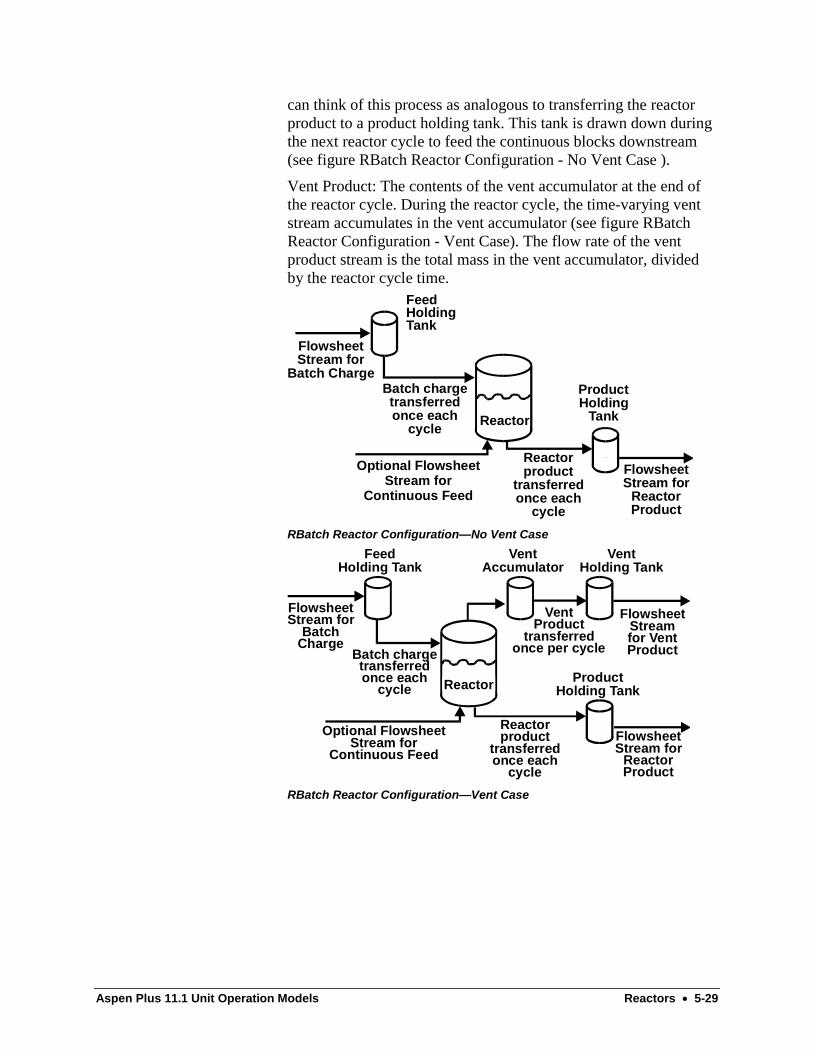
Aspen Plus 11.1 Unit Operation Models Reactors • 5-29
can think of this process as analogous to transferring the reactorproduct to a product holding tank. This tank is drawn down duringthe next reactor cycle to feed the continuous blocks downstream(see figure RBatch Reactor Configuration - No Vent Case ).
Vent Product: The contents of the vent accumulator at the end ofthe reactor cycle. During the reactor cycle, the time-varying ventstream accumulates in the vent accumulator (see figure RBatchReactor Configuration - Vent Case). The flow rate of the ventproduct stream is the total mass in the vent accumulator, dividedby the reactor cycle time.
FeedHoldingTank
FlowsheetStream for
Batch ChargeBatch chargetransferredonce each
cycle
ProductHolding
Tank
Reactorproduct
transferredonce each
cycle
FlowsheetStream for
ReactorProduct
Reactor
Optional FlowsheetStream for
Continuous Feed
RBatch Reactor Configuration—No Vent Case
FeedHolding Tank
FlowsheetStream for
BatchCharge
Batch chargetransferredonce each
cycleProduct
Holding Tank
Reactorproduct
transferredonce each
cycle
FlowsheetStream for
ReactorProduct
VentHolding Tank
VentAccumulator
VentProduct
transferredonce per cycle
FlowsheetStreamfor VentProduct
Reactor
Optional FlowsheetStream for
Continuous Feed
RBatch Reactor Configuration—Vent Case

5-30 • Reactors Aspen Plus 11.1 Unit Operation Models
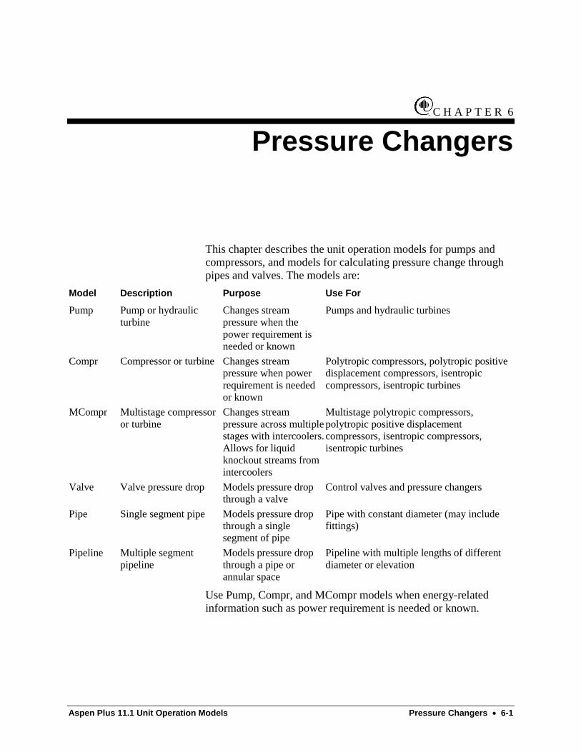
Aspen Plus 11.1 Unit Operation Models Pressure Changers • 6-1
C H A P T E R 6
Pressure Changers
This chapter describes the unit operation models for pumps andcompressors, and models for calculating pressure change throughpipes and valves. The models are:
Model Description Purpose Use For
Pump Pump or hydraulicturbine
Changes streampressure when thepower requirement isneeded or known
Pumps and hydraulic turbines
Compr Compressor or turbine Changes streampressure when powerrequirement is neededor known
Polytropic compressors, polytropic positivedisplacement compressors, isentropiccompressors, isentropic turbines
MCompr Multistage compressoror turbine
Changes streampressure across multiplestages with intercoolers.Allows for liquidknockout streams fromintercoolers
Multistage polytropic compressors,polytropic positive displacementcompressors, isentropic compressors,isentropic turbines
Valve Valve pressure drop Models pressure dropthrough a valve
Control valves and pressure changers
Pipe Single segment pipe Models pressure dropthrough a singlesegment of pipe
Pipe with constant diameter (may includefittings)
Pipeline Multiple segmentpipeline
Models pressure dropthrough a pipe orannular space
Pipeline with multiple lengths of differentdiameter or elevation
Use Pump, Compr, and MCompr models when energy-relatedinformation such as power requirement is needed or known.

6-2 • Pressure Changers Aspen Plus 11.1 Unit Operation Models
Pump ReferenceUse Pump to model a pump or a hydraulic turbine.
Pump is designed to handle a single liquid phase. For special cases,you can specify two- or three-phase calculations to determine theoutlet stream conditions and to compute the fluid density used inthe pump equations. The accuracy of the results depends on anumber of factors, such as the relative amounts of the phasespresent, the compressibility of the fluid, and the efficiencyspecified.
Use Pump to change pressure when the power requirement isneeded or known. For pressure change only, you can use othermodels such as Heater.
Pump can model pumps and hydraulic turbines.
Use the Pump block to rate a pump or a turbine by specifyingscalar parameters or by specifying the related performance curves.To use the performance curves, you can specify either:
• Dimensional curves such as head versus flow or power versusflow
• Dimensionless curves such as head coefficient versus flowcoefficient
Use the following forms to enter specifications and view results forPump:
Use this form To do this
Setup Specify operating conditions, efficiencies, netpositive suction head parameters, specific speedparameters, valid phases, and flash convergenceparameters
PerformanceCurves
Specify parameters and enter data for theperformance curves
UserSubroutine Specify name and parameters for the userperformance curve subroutine
BlockOptions Override global values for physical properties,simulation options, diagnostic message levels,and report options for this block
Results View summary of Pump results, material andenergy balance results, and performance curvesummary
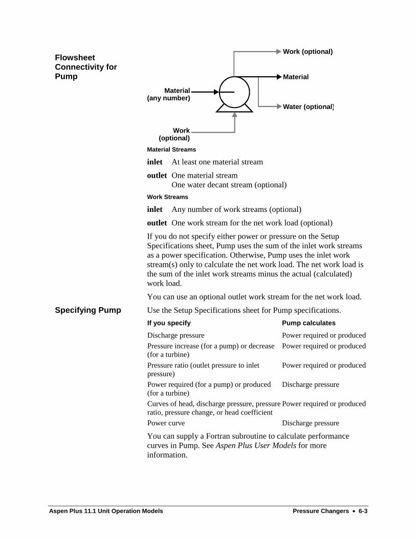
Aspen Plus 11.1 Unit Operation Models Pressure Changers • 6-3
Work(optional)
Material
Work (optional)
Water (optional)
Material(any number)
Material Streams
inlet At least one material stream
outlet One material streamOne water decant stream (optional)
Work Streams
inlet Any number of work streams (optional)
outlet One work stream for the net work load (optional)
If you do not specify either power or pressure on the SetupSpecifications sheet, Pump uses the sum of the inlet work streamsas a power specification. Otherwise, Pump uses the inlet workstream(s) only to calculate the net work load. The net work load isthe sum of the inlet work streams minus the actual (calculated)work load.
You can use an optional outlet work stream for the net work load.
Use the Setup Specifications sheet for Pump specifications.
If you specify Pump calculates
Discharge pressure Power required or produced
Pressure increase (for a pump) or decrease(for a turbine)
Power required or produced
Pressure ratio (outlet pressure to inletpressure)
Power required or produced
Power required (for a pump) or produced(for a turbine)
Discharge pressure
Curves of head, discharge pressure, pressureratio, pressure change, or head coefficient
Power required or produced
Power curve Discharge pressure
You can supply a Fortran subroutine to calculate performancecurves in Pump. See Aspen Plus User Models for moreinformation.
FlowsheetConnectivity forPump
Specifying Pump
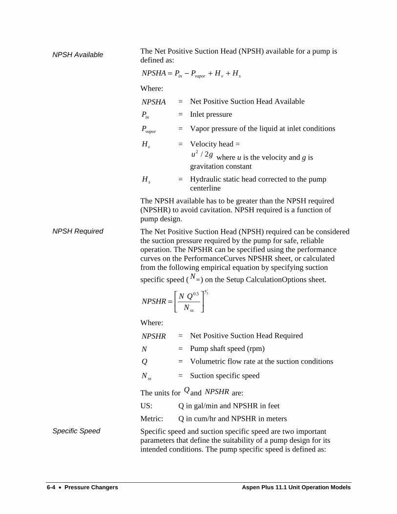
6-4 • Pressure Changers Aspen Plus 11.1 Unit Operation Models
The Net Positive Suction Head (NPSH) available for a pump isdefined as:
NPSHA P P H Hin vapor v s= − + +
Where:
NPSHA = Net Positive Suction Head Available
Pin = Inlet pressure
Pvapor = Vapor pressure of the liquid at inlet conditions
Hv = Velocity head =u g2 2/ where u is the velocity and g isgravitation constant
H s = Hydraulic static head corrected to the pumpcenterline
The NPSH available has to be greater than the NPSH required(NPSHR) to avoid cavitation. NPSH required is a function ofpump design.
The Net Positive Suction Head (NPSH) required can be consideredthe suction pressure required by the pump for safe, reliableoperation. The NPSHR can be specified using the performancecurves on the PerformanceCurves NPSHR sheet, or calculatedfrom the following empirical equation by specifying suction
specific speed ( N ss) on the Setup CalculationOptions sheet.
NPSHRN Q
N ss
=
0 54
3.
Where:
NPSHR = Net Positive Suction Head Required
N = Pump shaft speed (rpm)
Q = Volumetric flow rate at the suction conditions
N ss = Suction specific speed
The units for Qand NPSHR are:
US: Q in gal/min and NPSHR in feet
Metric: Q in cum/hr and NPSHR in meters
Specific speed and suction specific speed are two importantparameters that define the suitability of a pump design for itsintended conditions. The pump specific speed is defined as:
NPSH Available
NPSH Required
Specific Speed
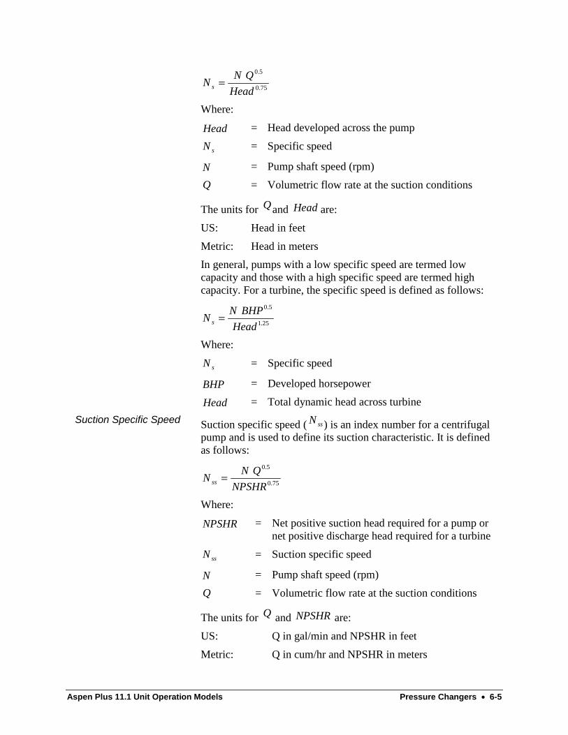
Aspen Plus 11.1 Unit Operation Models Pressure Changers • 6-5
NN Q
Heads =0 5
0 75
.
.
Where:
Head = Head developed across the pump
N s = Specific speed
N = Pump shaft speed (rpm)
Q = Volumetric flow rate at the suction conditions
The units for Qand Head are:
US: Head in feet
Metric: Head in meters
In general, pumps with a low specific speed are termed lowcapacity and those with a high specific speed are termed highcapacity. For a turbine, the specific speed is defined as follows:
NN BHP
Heads =0 5
1 25
.
.
Where:
N s = Specific speed
BHP = Developed horsepower
Head = Total dynamic head across turbine
Suction specific speed ( N ss) is an index number for a centrifugalpump and is used to define its suction characteristic. It is definedas follows:
NN Q
NPSHRss =0 5
0 75
.
.
Where:
NPSHR = Net positive suction head required for a pump ornet positive discharge head required for a turbine
N ss = Suction specific speed
N = Pump shaft speed (rpm)
Q = Volumetric flow rate at the suction conditions
The units for Q and NPSHR are:
US: Q in gal/min and NPSHR in feet
Metric: Q in cum/hr and NPSHR in meters
Suction Specific Speed
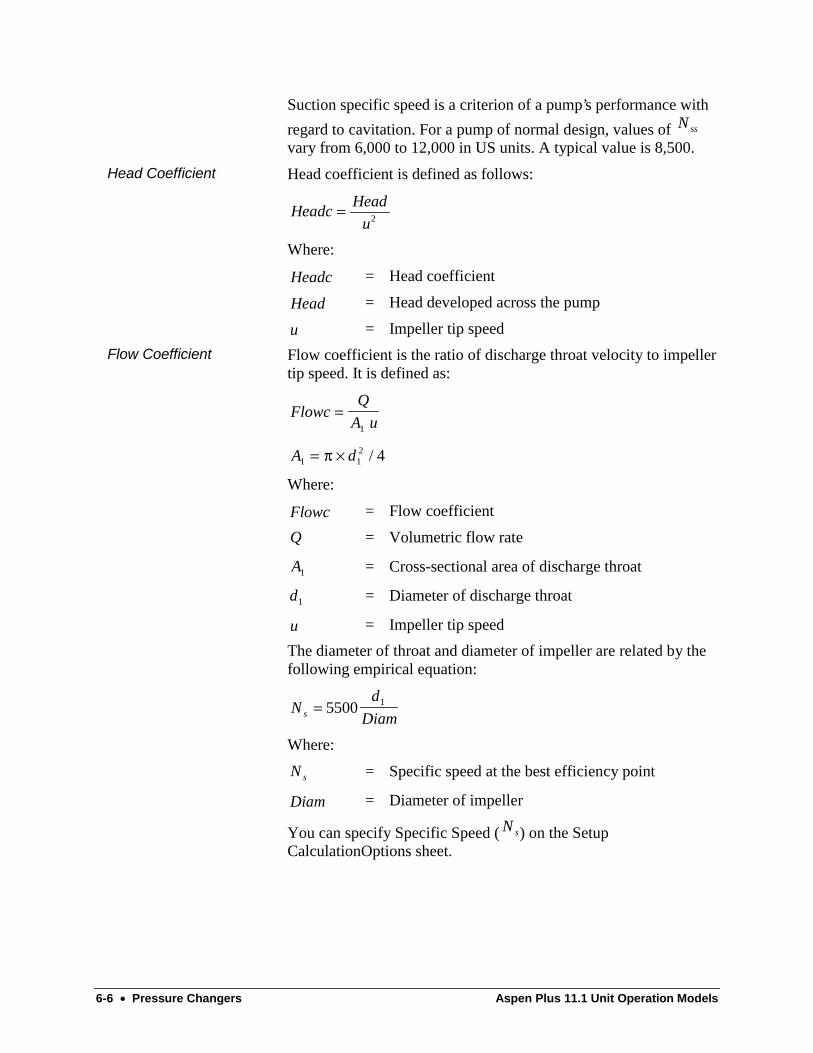
6-6 • Pressure Changers Aspen Plus 11.1 Unit Operation Models
Suction specific speed is a criterion of a pump’s performance with
regard to cavitation. For a pump of normal design, values of N ss
vary from 6,000 to 12,000 in US units. A typical value is 8,500.
Head coefficient is defined as follows:
HeadcHead
u=
2
Where:
Headc = Head coefficient
Head = Head developed across the pump
u = Impeller tip speed
Flow coefficient is the ratio of discharge throat velocity to impellertip speed. It is defined as:
FlowcQ
A u=
1
A d1 12 4= ×π /
Where:
Flowc = Flow coefficient
Q = Volumetric flow rate
A1 = Cross-sectional area of discharge throat
d1 = Diameter of discharge throat
u = Impeller tip speed
The diameter of throat and diameter of impeller are related by thefollowing empirical equation:
Nd
Diams = 5500 1
Where:
N s = Specific speed at the best efficiency point
Diam = Diameter of impeller
You can specify Specific Speed ( N s) on the SetupCalculationOptions sheet.
Head Coefficient
Flow Coefficient

Aspen Plus 11.1 Unit Operation Models Pressure Changers • 6-7
The performance curves can be entered in one of the followingcurve formats:
• Tabular data
• Polynomials
• User subroutine
You can select one of the following performance curves (thedependent variable) for the pump type you specified on the PumpSetup Specifications sheet:
Performance CurveType
Data for a pump Data for a turbine
Head Head required Head produced
Head-Coeff Head coefficient Head coefficient
Power Power required Power produced
Dis-Pressure Outlet pressure Outlet pressure
Pres-Ratio Pressure ratio Pressure ratio
Pres-Change Pressure increase Pressure decrease
The flow variable (the independent variable) can be one of thefollowing:
• Volume flow rate at suction conditions
• Mass flow rate at suction conditions
• Specific volumetric flow rate (for head coefficient only)
• Flow coefficient (for head coefficient only)
You can select one of the following options for specifying curves:
• A single curve at the operating shaft speed
• A single curve; use affinity laws to scale the performance froma reference speed
• Multiple curves at multiple shaft speeds
The features listed below are not supported in equation-orientedformulation. However, the capabilities are still available for the EOsolution strategy via the Perturbation Layer.
• Power, discharge pressure, and pressure-ratio performancecurves
• Multiple performance curves of other types
• Features which are globally unsupported
Single performance curves for head, head coefficient, and pressurechange are supported.
Performance Curves
EO Usage Notes forPump

6-8 • Pressure Changers Aspen Plus 11.1 Unit Operation Models
Compr ReferenceUse Compr to model:
• A polytropic centrifugal compressor
• A polytropic positive displacement compressor
• An isentropic compressor
• An isentropic turbine
Use Compr to change stream pressure when energy-relatedinformation, such as power requirement, is needed or known.
Compr can handle single-phase as well as two- and three-phasecalculations.
You can use Compr to rate a single stage of a compressor or asingle wheel of a compressor, by specifying the relatedperformance curves. Compr allows you to specify either:
• Dimensional curves, such as head versus flow or power versusflow
• Dimensionless curves, such as head coefficient versus flowcoefficient
Compr can also calculate compressor shaft speed.
Compr cannot handle performance curves for a turbine.
Use the following forms to enter specifications and view results forCompr:
Use this form To do this
Setup Identify compressor specifications, calculationoptions, convergence parameters, and validphases
PerformanceCurves
Specify parameters and enter data for theperformance curves
User Subroutine Enter performance curve subroutine parametersand name
Block Options Override global values for physical properties,simulation options, diagnostic message levels,and report options for this block
Results View summary of Compr results, material andenergy balance results, and performance curvesummary
Dynamic Specify parameters for dynamic simulations

Aspen Plus 11.1 Unit Operation Models Pressure Changers • 6-9
Material(any number)
Material
Water (optional)
Work(optional)
Work (optional)
Material Streams
inlet At least one material stream
outlet One material streamOne water decant stream (optional)
Work Streams
inlet Any number of work streams (optional)
outlet One work stream for net work load (optional)
If you do not specify either power or pressure on the Compr SetupSpecifications sheet, Compr uses the sum of the inlet work streamsas a power specification. Otherwise, Compr uses the inlet workstream(s) only to calculate the net work load. The net work load isthe sum of the inlet work streams minus the actual (calculated)work load.
You can use an optional outlet work stream for the net work load.
If you specify Compr calculates
Discharge pressure Power required or produced
Power required (for a compressor) orproduced (for a turbine)
Discharge pressure
Curves of head, power, dischargepressure, pressure ratio, pressurechange, or head coefficient
Power required and dischargepressure
Discharge pressure and curves of heador power or head coefficient
Power required, dischargepressure, and shaft speed
Power required and curves of dischargepressure, pressure ratio, or pressurechange
Discharge pressure, and shaftspeed
When you use performance curves, you can specify either a scalarvalue of efficiency or efficiency curves.
You can supply a Fortran subroutine to calculate performancecurves in Compr. See Aspen Plus User Models for moreinformation.
FlowsheetConnectivity forCompr
Specifying Compr

6-10 • Pressure Changers Aspen Plus 11.1 Unit Operation Models
Some required specifications depend on the compressor type.Specify the compressor type on the Setup Specifications sheet.
You can model a polytropic compressor using either the GPSA orASME method. You can model an isentropic compressor usingeither the GPSA, ASME, or Mollier-based methods. To model aturbine, you must use the Mollier-based method.
The GPSA method can be based on either:
• Suction conditions
• Average of suction and discharge conditions
The ASME method is more rigorous than the GPSA method forpolytropic or isentropic compressor calculations. The Molliermethod is the most rigorous for isentropic calculations.
The polytropic efficiency pη is used in the equation for the
polytropic compression ratio:
pk
k
n
n η
−=− 11
The basic compressor relation is:
−
−
=∆
−
11
1
n
n
in
out
p
inin
P
P
n
n
VPh
η
Where:
n = Polytropic coefficient
k = Heat capacity ratio Cp/Cv
pη = Polytropic efficiency
∆h = Enthalpy change per mole
P = Pressure
V = Molar volume
There are two equations for the isentropic efficiency sη
For compression:
inout
insout
s hh
hh
−−
=η
Polytropic Efficiency
Isentropic Efficiency

Aspen Plus 11.1 Unit Operation Models Pressure Changers • 6-11
For expansion:
insout
inouts
hh
hh
−−
=η
Where :
h = Molar enthalpy
houts = Outlet molar enthalpy assuming isentropic
compression or expansion to the specified outletpressure
Mechanical efficiency mη is used to calculate the brakehorsepower:
IHP F h= ∆
mIHPBHP η/=
Where:
IHP = Indicated horsepower
F = Mole flow rate
∆h = Enthalpy change per mole
BHP = Brake horsepower
mη = Mechanical efficiency
The head developed for a compressor to change the pressure of astream from the inlet pressure P1 to the outlet pressure P2 is givenby:
∫=2
1
p
pVdPHEAD
where V is the molar volume and subscripts 1 and 2 refer to inletand outlet conditions, respectively. Two integration methods areprovided for the polytropic and positive displacement modelcalculations using piecewise integration:
Direct method
Applying the gas law PV = ZRT and using the average point foreach interval, given the number of intervals between P1 and P2,subpath i for head developed can be written as:
=
i
i
avi
P
PZTRHEAD
1
2ln)(
Mechanical Efficiency
Integration Method
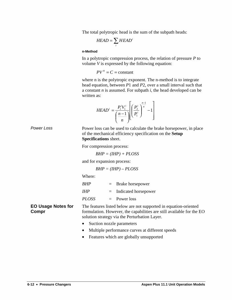
6-12 • Pressure Changers Aspen Plus 11.1 Unit Operation Models
The total polytropic head is the sum of the subpath heads:i
i
EADHHEAD ∑=
n-Method
In a polytropic compression process, the relation of pressure P tovolume V is expressed by the following equation:
constant== CPV n
where n is the polytropic exponent. The n-method is to integratehead equation, between P1 and P2, over a small interval such thata constant n is assumed. For subpath i, the head developed can bewritten as:
−
−
=
−
11
1
1
211n
n
i
iiii
P
P
n
n
VPHEAD
Power loss can be used to calculate the brake horsepower, in placeof the mechanical efficiency specification on the SetupSpecifications sheet.
For compression process:
BHP = (IHP) + PLOSS
and for expansion process:
BHP = (IHP) – PLOSS
Where:
BHP = Brake horsepower
IHP = Indicated horsepower
PLOSS = Power loss
The features listed below are not supported in equation-orientedformulation. However, the capabilities are still available for the EOsolution strategy via the Perturbation Layer.
• Suction nozzle parameters
• Multiple performance curves at different speeds
• Features which are globally unsupported
Power Loss
EO Usage Notes forCompr

Aspen Plus 11.1 Unit Operation Models Pressure Changers • 6-13
MCompr ReferenceUse MCompr to model:
• A multi-stage polytropic compressor
• A multi-stage polytropic positive displacement compressor
• A multi-stage isentropic compressor
• A multi-stage isentropic turbine
For polytropic compressors, MCompr can handle a single,compressible phase. For special cases you can specify two- orthree-phase calculations. These calculations determine the outletstream conditions and the properties used in the compressorequations. The accuracy of results depends primarily on therelative amounts of the phases present and the efficiency specified.The rigorous polytropic compressor uses real fluid propertiescalculated from the property method you specify. It does notassume ideal gas behavior.
MCompr handles single-phase isentropic compressors andturbines. MCompr can also handle two- and three-phase mixtures.
You can use MCompr to rate a multi-stage compressor, by usingeither:
• Stage-by-stage dimensional performance curves, such as headversus flow or power versus flow
• Wheel-by-wheel dimensionless performance curves, such ashead coefficient versus flow coefficient
MCompr can also calculate shaft speed.
MCompr cannot handle performance curves for a turbine.

6-14 • Pressure Changers Aspen Plus 11.1 Unit Operation Models
Use the following forms to enter specifications and view results forMCompr:
Use this form To do this
Setup Identify multi-stage compressor specifications, stagespecifications, cooler specifications, convergenceparameters, and valid phases
PerformanceCurves
Specify parameters and enter data for theperformance curves
User Subroutine Specify performance curve user subroutineparameters and name
Hcurves Specify heating or cooling curve tables and viewtabular results
Block Options Override global values for physical properties,simulation options, diagnostic message levels, andreport options for this block
Results View summary of operating results, material andenergy balance results, compressor and coolerprofiles, and performance profiles
Dynamic Specify parameters for dynamic simulations
Heat(optional)
Work(optional)
Work(any number)
ToStageK + 1
FromStageK - 1
Feed toStageK + 1(any number)
Heat(any number)
Water(optional)
KnockoutStage K
Cooler
Stage KCompressor
Stage K
Material Streams
inlet At least one material stream for the first compressor stageOne or more material streams for stages after the first(optional). These streams enter the intercooler before thestages you specify.
outlet One material stream leaving the last compressor stageEither one optional knockout material stream for eachintercooler for the liquid formed, or one optional globalknockout for the liquid formed in all intercoolersEither one optional water decant stream for eachintercooler, or one optional global water decant stream
FlowsheetConnectivity forMCompr

Aspen Plus 11.1 Unit Operation Models Pressure Changers • 6-15
If you use liquid knockout outlet streams from one stage, you mustuse them for all stages. The last stage cannot have a liquidknockout material stream or a water decant stream.
Heat Streams
inlet Any number of heat streams to each intercooler (optional)
outlet Either one optional heat stream for the net heat load of eachintercooler, or one global heat outlet stream for the net heatduty for all intercoolers
If you do not specify cooler conditions on the Setup Cooler sheet,MCompr adds the heat streams together and uses the total as a dutyspecification for the cooler.
The net heat load equals the heat in the inlet heat streams minusthe actual (calculated) heat duty.
If you use a heat outlet from one stage, you must use one for allstages.
Work Streams
inlet Any number of work streams to each compressor stage(optional)
outlet Either one optional work stream for net work load, or oneglobal work stream for the net power for all compressorstages
MCompr adds all work inlet streams together to provide the powerrequirement. If you do not specify power or pressure on the SetupSpecs sheet, MCompr uses the total power as a power specificationfor the stage.
The power in the outlet work stream equals the power in the inletwork streams minus the actual (calculated) power required.
If you use a work outlet from one stage, you must use one for allstages.
If you specify MCompr calculates
Discharge pressure Power required or produced
Power required (for a compressor) orproduced (for a turbine)
Discharge pressure
Curves of head, power, dischargepressure, pressure ratio, pressurechange, or head coefficient
Power required and dischargepressure
Discharge pressure and curves of heador power or head coefficient
Power required, and shaft speed
When you use performance curves, you can specify either a scalarvalue for efficiency or efficiency curves.
Specifying MCompr
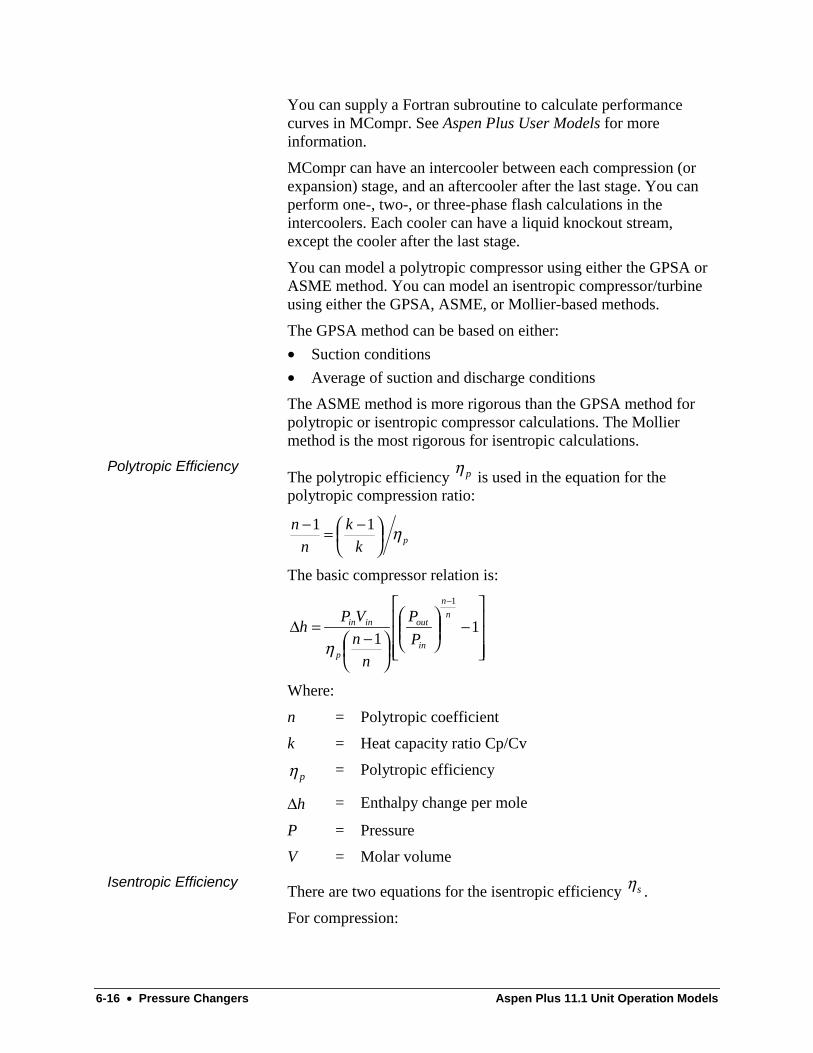
6-16 • Pressure Changers Aspen Plus 11.1 Unit Operation Models
You can supply a Fortran subroutine to calculate performancecurves in MCompr. See Aspen Plus User Models for moreinformation.
MCompr can have an intercooler between each compression (orexpansion) stage, and an aftercooler after the last stage. You canperform one-, two-, or three-phase flash calculations in theintercoolers. Each cooler can have a liquid knockout stream,except the cooler after the last stage.
You can model a polytropic compressor using either the GPSA orASME method. You can model an isentropic compressor/turbineusing either the GPSA, ASME, or Mollier-based methods.
The GPSA method can be based on either:
• Suction conditions
• Average of suction and discharge conditions
The ASME method is more rigorous than the GPSA method forpolytropic or isentropic compressor calculations. The Molliermethod is the most rigorous for isentropic calculations.
The polytropic efficiency pη is used in the equation for the
polytropic compression ratio:
pk
k
n
n η
−=− 11
The basic compressor relation is:
−
−
=∆
−
11
1
n
n
in
out
p
inin
P
P
n
n
VPh
η
Where:
n = Polytropic coefficient
k = Heat capacity ratio Cp/Cv
pη = Polytropic efficiency
∆h = Enthalpy change per mole
P = Pressure
V = Molar volume
There are two equations for the isentropic efficiency sη .
For compression:
Polytropic Efficiency
Isentropic Efficiency

Aspen Plus 11.1 Unit Operation Models Pressure Changers • 6-17
inout
insout
s hh
hh
−−
=η
For expansion:
insout
inouts hh
hh
−−
=η
Where :
h = Molar enthalpy
houts = Outlet molar enthalpy assuming isentropic
compression or expansion to the specified outletpressure
Mechanical efficiency mη is used to calculate the brakehorsepower:
IHP F h= ∆
mIHPBHP η/=
Where:
IHP = Indicated horsepower
F = Mole flow rate
∆h = Enthalpy change per mole
BHP = Brake horsepower
mη = Mechanical efficiency
The parasitic pressure loss at the suction of a stage is calculatedusing the equation:
∆P KV
= ρ2
2
Where:
∆P = Parasitic pressure loss
K = Velocity head multiplier
ρ = Density
V = Linear velocity of process gas at suction conditions
The specific speed is defined as:
SpSpd = ShSpd (VflIn)
(Head)
0.5
0.75
Mechanical Efficiency
Parasitic Pressure Loss
Specific Speed

6-18 • Pressure Changers Aspen Plus 11.1 Unit Operation Models
Where:
ShSpd = Shaft speed
VflIn = Suction volumetric flow rate
Head = Head developed
The specific diameter is defined as:
SpDiam = ImpDiam (Head)
(VflIn)
0.25
0.5
Where:
ImpDiam = Impeller diameter of compressor wheel
Head = Head developed
VflIn = Volumetric flow rate at suction conditions
The head coefficient is defined as:
Hc = Head
( ShSpd ImpDiam)
2π
Where:
Head = Head developed
π = 3.1416
ShSpd = Shaft speed
ImpDiam = Impeller diameter of compressor wheel
The flow coefficient is defined as:
FcVflIn
ShSpd (ImpDiam=
)3
Where:
VflIn = Volumetric flow rate at suction conditions
ShSpd = Shaft speed
ImpDiam = Impeller diameter of compressor wheel
GPSA Engineering Data Book, 1979, Chapter 4, pp. 5-6 to 5-10.
ASME Power Test Code 10, 1965, pp. 31-32.
Specific Diameter
Head Coefficient
Flow Coefficient
References

Aspen Plus 11.1 Unit Operation Models Pressure Changers • 6-19
Valve ReferenceValve models control valves and pressure changers. Valve relatesthe pressure drop across a valve to the valve flow coefficient.Valve assumes the flow is adiabatic, and determines the thermaland phase condition of the stream at the valve outlet. Valve canperform one-, two-, or three-phase calculations.
Use the following forms to enter specifications and view results forValve:
Use this form To do this
Input Specify valve operating conditions, flashconvergence parameters, valid phases, valveparameters, sizes for pipe fittings, calculationoptions, and Valve convergence parameters
Block Options Override global values for physical properties,simulation options, diagnostic message levels,and report options for this block
Results View summary of operating results and mass andenergy balances
Material Material
Material Streams
inlet One material stream
outlet One material stream
Use the Input Operation sheet to select the calculation type.
If you select the Pressure changer option or the Design option forthe calculation type, you must specify, on the same sheet, one ofthe following:
• Outlet pressure
• Pressure drop
If you select the Pressure changer option, the specification iscomplete and Valve performs an adiabatic flash to calculate thethermal and phase condition of the outlet stream.
FlowsheetConnectivity forValve
Specifying Valve
6-20 • Pressure Changers Aspen Plus 11.1 Unit Operation Models
If you select the Rating option for the calculation type, you mustspecify, on the same sheet, one of the following:
• Flow coefficient at operating valve position
• Valve operating position (% Opening)
If you specify the valve operating position, you must also specifyone of the following on the Input ValveParameters sheet:
• Characteristic equation type and flow coefficient at maximumvalve opening
• Data for flow coefficient (Cv) versus valve opening in theValve Parameters Table
• A valve from the built-in library based on valve type,manufacturer, series/style, and size
On the Input CalculationOptions sheet, you can specify that Valve:
• Check for choked flow
• Calculate cavitation index
For vapor-containing streams, you must specify the pressure dropratio factor (Xt) for the valve. For liquid-containing streams, if youspecify that Valve check for choked flow, you must also specifythe pressure recovery factor (Fl) for the valve. You can specify thepressure drop ratio factor and the pressure recovery factor for thevalve in one of the following ways on the Input ValveParameterssheet:
Specify
• Value at the operating valve position (Pres Drop Ratio Factor,Pres Recovery Factor)
• Data for pressure drop ratio factor (Xt) and for pressurerecovery factor (Fl) versus valve opening (% Opening) in theValve Parameters Table
• A valve from the built-in library based on Valve Type,Manufacturer, Series/Style, and Size
If you want to include the effect of head loss from pipe fittings onthe valve flow capacity, you must specify the diameters of thevalve and pipe fittings on the Input PipeFittings sheet. Valve usesthe valve and pipe diameters, and estimates the piping geometryfactor to account for the reduction in flow capacity.
The pressure drop ratio factor ( Xt ) accounts for the effect of theinternal geometry of the valve on the change in fluid density as itpasses through the valve.
The pressure drop ratio factor is the limiting value (under chokedconditions) of the pressure drop ratio and is given by:
Pressure Drop RatioFactor
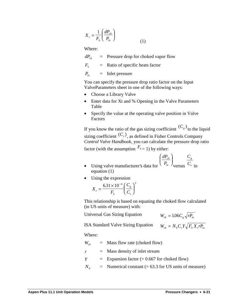
Aspen Plus 11.1 Unit Operation Models Pressure Changers • 6-21
XF
dP
Ptk
ch
in
=
1
(1)
Where:
dPch = Pressure drop for choked vapor flow
Fk = Ratio of specific heats factor
Pin = Inlet pressure
You can specify the pressure drop ratio factor on the InputValveParameters sheet in one of the following ways:
• Choose a Library Valve
• Enter data for Xt and % Opening in the Valve ParametersTable
• Specify the value at the operating valve position in ValveFactors
If you know the ratio of the gas sizing coefficient ( )Cg to the liquid
sizing coefficient ( )Cv , as defined in Fisher Controls CompanyControl Valve Handbook, you can calculate the pressure drop ratio
factor (with the assumption Fk = 1) by either:
• Using valve manufacturer’s data for
dP
Pch
in
versus
C
Cg
v inequation (1)
• Using the expression
XF
C
Ctk
g
v
=×
−6 31 10 4 2.
This relationship is based on equating the choked flow calculated(in US units of measure) with:
Universal Gas Sizing Equation W C rPch g in= 106.
ISA Standard Valve Sizing Equation W N C Y F X rPch v k t in= 6
Where:
Wch = Mass flow rate (choked flow)
r = Mass density of inlet stream
Y = Expansion factor (= 0.667 for choked flow)
N 6 = Numerical constant (= 63.3 for US units of measure)
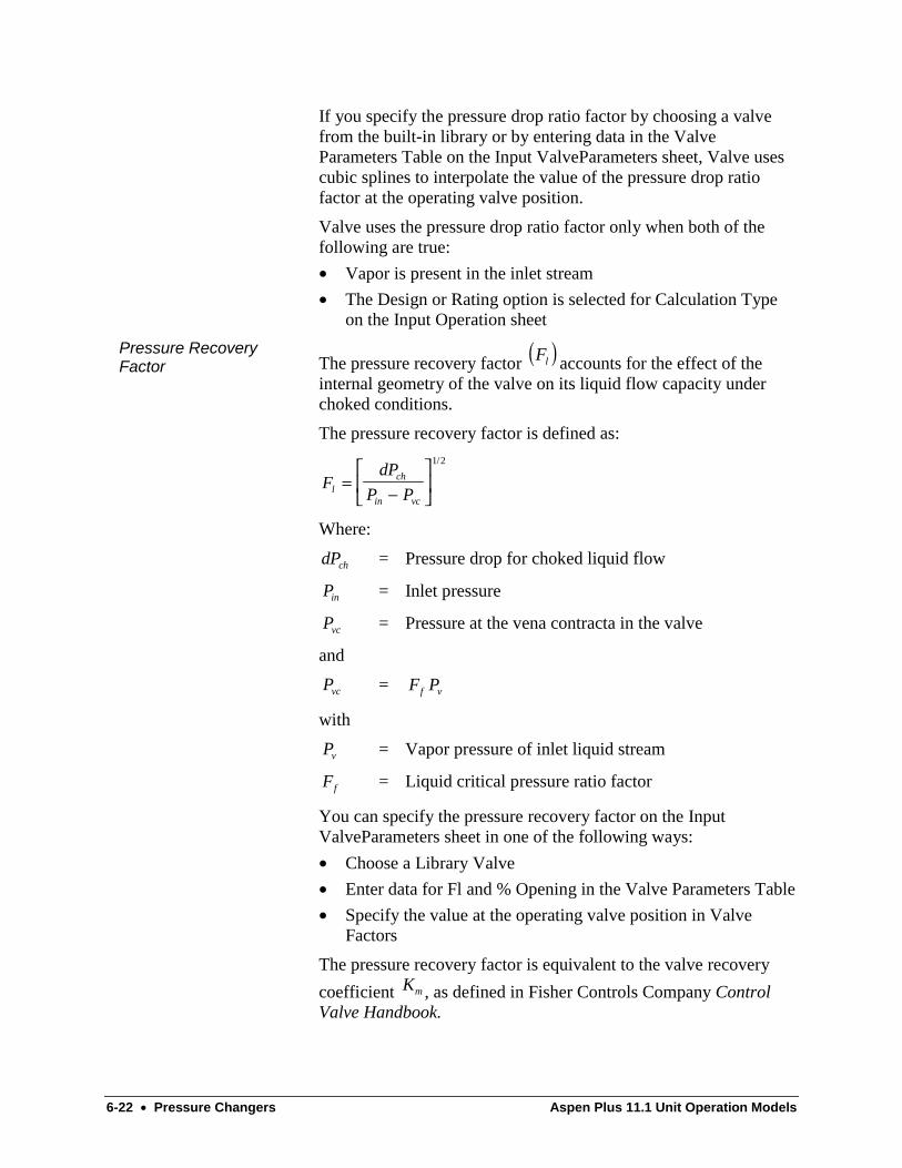
6-22 • Pressure Changers Aspen Plus 11.1 Unit Operation Models
If you specify the pressure drop ratio factor by choosing a valvefrom the built-in library or by entering data in the ValveParameters Table on the Input ValveParameters sheet, Valve usescubic splines to interpolate the value of the pressure drop ratiofactor at the operating valve position.
Valve uses the pressure drop ratio factor only when both of thefollowing are true:
• Vapor is present in the inlet stream
• The Design or Rating option is selected for Calculation Typeon the Input Operation sheet
The pressure recovery factor ( )Fl accounts for the effect of theinternal geometry of the valve on its liquid flow capacity underchoked conditions.
The pressure recovery factor is defined as:
FdP
P Plch
in vc
=−
1 2/
Where:
dPch = Pressure drop for choked liquid flow
Pin = Inlet pressure
Pvc = Pressure at the vena contracta in the valve
and
Pvc = F Pf v
with
Pv = Vapor pressure of inlet liquid stream
Ff = Liquid critical pressure ratio factor
You can specify the pressure recovery factor on the InputValveParameters sheet in one of the following ways:
• Choose a Library Valve
• Enter data for Fl and % Opening in the Valve Parameters Table
• Specify the value at the operating valve position in ValveFactors
The pressure recovery factor is equivalent to the valve recovery
coefficient Km , as defined in Fisher Controls Company ControlValve Handbook.
Pressure RecoveryFactor
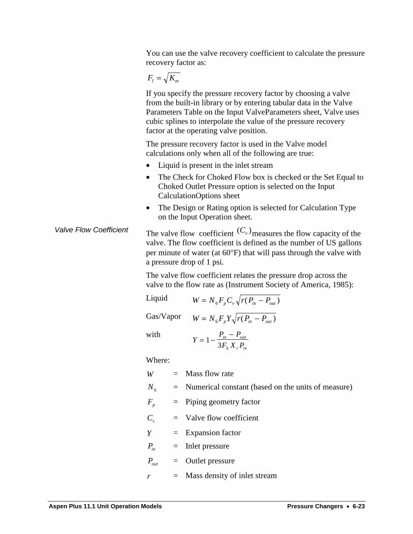
Aspen Plus 11.1 Unit Operation Models Pressure Changers • 6-23
You can use the valve recovery coefficient to calculate the pressurerecovery factor as:
F Kl m=
If you specify the pressure recovery factor by choosing a valvefrom the built-in library or by entering tabular data in the ValveParameters Table on the Input ValveParameters sheet, Valve usescubic splines to interpolate the value of the pressure recoveryfactor at the operating valve position.
The pressure recovery factor is used in the Valve modelcalculations only when all of the following are true:
• Liquid is present in the inlet stream
• The Check for Choked Flow box is checked or the Set Equal toChoked Outlet Pressure option is selected on the InputCalculationOptions sheet
• The Design or Rating option is selected for Calculation Typeon the Input Operation sheet.
The valve flow coefficient ( )Cv measures the flow capacity of thevalve. The flow coefficient is defined as the number of US gallonsper minute of water (at 60°F) that will pass through the valve witha pressure drop of 1 psi.
The valve flow coefficient relates the pressure drop across thevalve to the flow rate as (Instrument Society of America, 1985):
Liquid W N F C r P Pp v in out= −6 ( )
Gas/Vapor W N F Y r P Pp in out= −6 ( )
withY
P P
F X Pin out
k t in
= −−
13
Where:
W = Mass flow rate
N 6 = Numerical constant (based on the units of measure)
Fp = Piping geometry factor
Cv = Valve flow coefficient
Y = Expansion factor
Pin = Inlet pressure
Pout = Outlet pressure
r = Mass density of inlet stream
Valve Flow Coefficient

6-24 • Pressure Changers Aspen Plus 11.1 Unit Operation Models
Fk = Ratio of specific heats factor
X t = Pressure drop ratio factor
You can specify the flow coefficient in one of the following ways:
• Use Flow Coef on the Input Operation sheet to specify thevalue at the operating valve position
• Choose a Library Valve on the Input ValveParameters sheet
• Enter data for Cv and % Opening in the Valve ParametersTable on the Input ValveParameters sheet
• Specify Valve Characteristics in the Input ValveParameterssheet
If you specify the flow coefficient by choosing a valve from thebuilt-in library or by entering data in the Valve Parameters Table,Valve uses cubic splines to interpolate the value of the flowcoefficient at the operating valve position.
The characteristic equation for the valve relates the flowcoefficient to the valve opening. Use the Input ValveParameterssheet to specify the characteristic equation type. The six built-incharacteristic equations are:
Type Equation
Linear V P=Parabolic V P= 0 01 2.Square Root
V P= 10 0.Quick Opening
( )V
P
P=
+ × −
10 0
10 9 9 10 3 2
.
. .
Equal PercentageV
P
P=
− × −
0 01
2 0 10 10
2
8 4
.
. .Hyperbolic
( )V
P
P=
− × −
01
10 9 9 10 5 2
.
. .
Where:
P = Valve opening as a percentage of maximum opening
V = Flow coefficient as a percentage of flow coefficient atmaximum opening
The piping geometry factor is defined as:
FC
Cpp= υ
υ
Characteristic EquationType
Piping Geometry Factor

Aspen Plus 11.1 Unit Operation Models Pressure Changers • 6-25
Where:
C pυ = Flow coefficient of the valve with attached fittings
Cυ = Flow coefficient of the valve installed in a straightpipe of the same size
The piping geometry factor accounts for the reduction in the flowcapacity of a valve due to the head loss from the pipe fittings. Thepiping geometry factor has a default value of 1.0 if the valve andpipe fittings have the same diameter.
Aspen Plus calculates the piping geometry factor as (InstrumentSociety of America, 1985):
FKC
N dp = +
−
Σ 2
24
0 5
1υ
.
with ΣK K K K KB B= + + −1 2 1 2
Where:
Kd
D1
2
12
2
05 1= −
.
, K
d
D2
2
22
2
10 1= −
.
, K
d
DB11
4
1= −
,
Kd
DB22
4
1= −
and:
Fp = Piping geometry factor
Cυ = Valve flow coefficient
N2 = Numerical constant (based on the units ofmeasure)
d = Valve diameter
K K1 2, = Resistance coefficients of the inlet and outletfittings
K KB B1 2, = Bernoulli coefficients for the inlet and outletfittings
D1 = Inlet pipe diameter
D2 = Outlet pipe diameter
If the valve and pipe fittings diameters are different and you wishto include the effect of the additional head loss on the valve flow
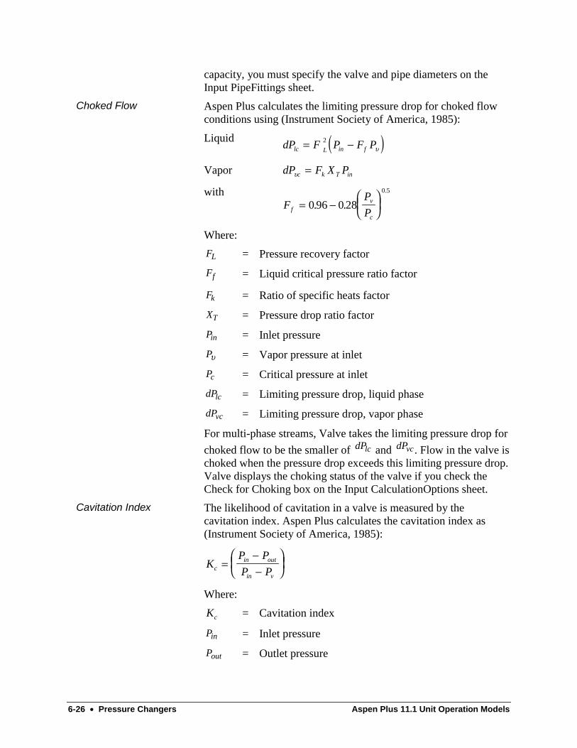
6-26 • Pressure Changers Aspen Plus 11.1 Unit Operation Models
capacity, you must specify the valve and pipe diameters on theInput PipeFittings sheet.
Aspen Plus calculates the limiting pressure drop for choked flowconditions using (Instrument Society of America, 1985):
Liquid ( )dP F P F Plc L in f= −2υ
Vapor dP F X Pc k T inυ =
withF
P
Pfv
c
= −
0 96 0 28
0 5
. .
.
Where:
FL = Pressure recovery factor
Ff = Liquid critical pressure ratio factor
Fk = Ratio of specific heats factor
XT = Pressure drop ratio factor
Pin = Inlet pressure
Pυ = Vapor pressure at inlet
Pc = Critical pressure at inlet
dPlc = Limiting pressure drop, liquid phase
dPvc = Limiting pressure drop, vapor phase
For multi-phase streams, Valve takes the limiting pressure drop for
choked flow to be the smaller of dPlc and dPvc . Flow in the valve ischoked when the pressure drop exceeds this limiting pressure drop.Valve displays the choking status of the valve if you check theCheck for Choking box on the Input CalculationOptions sheet.
The likelihood of cavitation in a valve is measured by thecavitation index. Aspen Plus calculates the cavitation index as(Instrument Society of America, 1985):
KP P
P Pcin out
in v
=−−
Where:
Kc = Cavitation index
Pin = Inlet pressure
Pout = Outlet pressure
Choked Flow
Cavitation Index

Aspen Plus 11.1 Unit Operation Models Pressure Changers • 6-27
Pv = Vapor pressure at inlet
The cavitation index definition is valid only for all-liquid streams.Valve calculates the cavitation index if you check the CalculateCavitation Index box on the Input CalculationOptions sheet.
Flow Equations for Sizing Control Valves, ISA-S75.01-1985,Instrument Society of America, 1985.
Reference
6-28 • Pressure Changers Aspen Plus 11.1 Unit Operation Models
Pipe ReferencePipe calculates the pressure drop and heat transfer in a singlesegment pipe. You can also use Pipe to model the pressure dropdue to fittings.
Pipe handles a single inlet and outlet material stream. Pipe assumesthe flow is one-dimensional, steady-state, and fully developed (thatis, no entrance effects are modeled). Pipe can perform one-, two-,or three-phase calculations. Flow direction and elevation angle arearbitrary.
To model multiple pipe segments of different diameters orelevations, use Pipeline instead of Pipe.
If the inlet pressure is known, Pipe calculates the outlet pressure. Ifthe outlet pressure is known, Pipe calculates the inlet pressure andupdates the state variables of the inlet stream.
Use Pipe to:
• Calculate inlet or discharge conditions
• Calculate pressure drops for one-, two-, or three-phase vaporand liquid flows
Use the following forms to enter specifications and view results forPipe:
Use this form To do this
Setup Specify pipe parameters, thermal specifications,fittings, flash convergence parameters andproperty profiles to be reported
Advanced Specify calculation options, solution methods,property grid, integration parameters and Beggsand Brill coefficients
UserSubroutine Specify pressure drop and/or holdup and/ordiameter calculation user subroutine name andparameters
Dynamic Specify parameters for dynamic simulations
BlockOptions Override global values for physical properties,simulation options, diagnostic message levels,and report options for this block
Results View summary of Pipe results, inlet and outletstream results, material and energy balanceresults, and profiles

Aspen Plus 11.1 Unit Operation Models Pressure Changers • 6-29
Material
MaterialMaterial Streams
inlet One material stream
outlet One material stream
You must specify the following for Pipe:
• Pipe length, diameter, roughness, and angle on the SetupPipeParameters sheet
• Thermal specification type on the Setup ThermalSpecificationsheet to determine whether Pipe operates with a temperatureprofile or temperature is calculated
• Whether to integrate, assume constant dP/dL, or use a closedform equation on the Advanced Methods sheet
• Frictional and holdup correlation when a closed form equationis not used on the Advanced Methods sheet
• Pressure and temperature grid for fluid property calculations onthe Advanced PropertyGrid sheet, if you request a pressure-temperature grid on the AdvancedCalculation Options sheet
• Integration direction in which calculations proceed with respectto flow on the Advanced CalculationOptions sheet
If the option selectedis
Pipe needs the And the integrationdirection is
Calculate pipe outletpressure(default)
Inlet pressure Downstream
Calculate pipe inletpressure
Outlet pressure Upstream
Pipe uses the inlet or outlet stream pressure to start thecalculations. If the stream is an external feed to your flowsheet, orthe outlet of a block that will execute after Pipe, use the StreamSpecifications sheet to specify the stream pressure. If theintegration direction is upstream, you can also specify the initialpressure for Pipe on the Advanced CalculationOptions sheet, byentering the outlet pressure. This pressure value will override thestream pressure entered on the Stream Specifications sheet.
FlowsheetConnectivity for Pipe
Specifying Pipe
6-30 • Pressure Changers Aspen Plus 11.1 Unit Operation Models
Select the flow calculation option on the AdvancedCalculationOptions sheet to specify whether Pipe is to calculate theoutlet or inlet stream flow and composition.
If the option selected is Pipe needs the
Reference inlet stream (default) Inlet flow and composition
Use outlet stream flow Outlet flow and composition
You must initialize the inlet stream to Pipe whenever the option toreference inlet stream is selected, even if the inlet pressure is beingcalculated. Similarly, you must initialize the outlet streamwhenever the option to use the outlet stream flow is selected. Theinitialized stream must be one of the following:
• Entered on a Stream Specifications sheet
• An outlet stream from part of the flowsheet executed (if optionto use outlet stream flow is selected)
• Transferred from another part of a flowsheet using a Transferblock
You can specify that a rigorous flash is to be performed each timeproperties are calculated, by selecting the option to do Flash atEach Integration Step on the Advanced CalculationOptions sheet.If you select the option to Interpolate from Property Grid, Pipe willdetermine properties by interpolating in a table of property valuesat various temperatures and pressures. Specify one of the followingif you use the Property Grid:
• A range of temperatures and pressures on the AdvancedProperty Grid sheet. Pipe will calculate properties at theseconditions and interpolate
• The block ID of a Pipe block for which the option tointerpolate from property grid was also selected, and whichwill be executed before the current block in the flowsheet
Pipe can calculate pressure drop for either one-, two-, or three-phase vapor and liquid flows. If vapor-liquid flow exists, Pipe alsocalculates liquid holdup and flow regime (pattern). You mayspecify a flowing fluid temperature profile, or Pipe can determineit from heat transfer calculations. Pipe treats multiple liquid phases(for example, oil and water) as a single homogeneous liquid phasefor pressure-drop and holdup calculations. Pipe automaticallydetects the special case of a single component fluid (for example,steam) and treats it appropriately.
For downstream and upstream integration, the combination ofoptions selected for pressure and flow calculation on the AdvancedCalculationOptions sheet determine which stream Pipe will update.The following table describes the available combinations. The next
Stream Specification
Physical PropertyCalculations
Pressure DropCalculations
Downstream andUpstream Integration

Aspen Plus 11.1 Unit Operation Models Pressure Changers • 6-31
figure, Downstream and Upstream Integration, defines the inletand outlet stream and pressure variables:
If the pressurecalculation option is
And the flowcalculation option is
Then Pipe updates the
Calculate pipe outletpressure
Calculate outletstream flow
Outlet stream only
Calculate pipe outletpressure
Calculate inlet streamflow
Outlet streamthermodynamic conditions
Inlet stream compositionand flow
Calculate pipe inletpressure
Calculate inlet streamflow
Inlet stream only
Calculate pipe inletpressure
Calculate outletstream flow
Inlet stream thermodynamicconditions
Outlet stream compositionand flow
Inlet Stream
Inlet Pressure Outlet Pressure
Outlet Stream
Downstream and Upstream Integration
Use caution when using Pipe inside a Design-Spec convergenceloop. For example, you can manipulate the flow rate to a pipe toachieve a desired pipe outlet pressure. During the designspecification convergence, the flow rate variables may becomeunreasonable in an intermediate iteration, causing Pipe to predict anegative pressure. Convergence difficulties occur as a result. Youcan avoid this situation by doing one of the following:
• Keep the upper limit of the flow rate sufficiently low inDesign-Spec
• Perform an upstream integration from the known outletpressure. Select option to calculate pipe inlet pressure on theAdvanced CalculationOptions sheet for this purpose. Define aDesign-Spec to manipulate the flow rate to achieve thespecified inlet pressure.
Erosional velocity is the velocity of the fluid in the pipe, abovewhich the pipe material will start to break off. The fluid istraveling so fast that it starts to strip material from the walls of thepipe. In general use, the flow rate should be below this value.
You can specify the erosional velocity coefficient on the SetupPipe Parameters sheet.
Design-SpecConvergence Loop
Erosional Velocity
6-32 • Pressure Changers Aspen Plus 11.1 Unit Operation Models
The erosional velocity is related to the erosional velocitycoefficient by the following equation:
ρυ c
c =
Where:
υc = Erosional velocity in ft/second
c = Erosional velocity coefficient(default=100)
ρ = Density in lbs/cubic ft
Gas systems consisting mostly of methane occur frequently in thedense-phase region of wellbores and flowlines. In the dense-phaseregion, definable vapor and liquid phases do not exist. Equation-of-state methods classify the dense-phase material as either allvapor or all liquid. Significant differences in the predicted fluidtransport properties may occur, depending on whether you choosethe vapor or liquid state.
Experience has shown that gas system flow in the dense-phaseregion is best modeled by using vapor-phase properties. Forsystems consisting of mostly methane, where the pipe conditionslie above the cricondenbar of the phase envelope, specify vapor-only valid phase on the Setup FlashOptions sheet.
Pipe assumes that the pressure drop due to valves and fittings isdistributed evenly along the specified length of the pipe. The totallength Pipe uses in calculations corresponds to the specified pipelength, plus any equivalent pipe length due to valves, fittings, andmiscellaneous L/D.
If the pipe is not horizontal, Pipe adjusts the angle from thehorizontal to achieve the same vertical rise or fall for the totallength used in the calculations. This adjustment ensures the correctpressure drop due to elevation.
If the order and position of the valves and fittings are important,you need to model each valve and fitting separately with a Pipemodel, specifying zero length of pipe.
See Pipeline reference for information on Two-Phase Friction-Factor and Liquid-Holdup Correlations and Closed Form Methods.
Methane Gas Systems
Modeling Valves andFittings
Two-PhaseCorrelations
Aspen Plus 11.1 Unit Operation Models Pressure Changers • 6-33
Pipeline ReferenceUse Pipeline to calculate the pressure drop in a straight pipe orannular space. Pipeline can:
• Simulate a piping network with successive blocks, includingwellbores and flowlines
• Contain any number of segments within each block to describepipe geometry
• Calculate inlet or discharge conditions
• Calculate pressure drops for one-, two-, or three-phase vaporand liquid flows. Pipeline treats multiple liquid phases (forexample, oil and water) as a single homogeneous liquid phasefor pressure-drop and holdup calculations. If vapor-liquid flowexists, Pipeline calculates liquid holdup and flow regime(pattern).
You may specify a flowing fluid temperature profile, or Pipelinecan calculate it from heat transfer calculations. Flow is assumed tobe one-dimensional, steady-state, and fully developed (no entranceeffects are modeled). Flow direction and elevation angle arearbitrary. To model a single pipe segment with constant diameterand elevation, you can also use Pipe.
Use the following forms to enter specifications and view results forPipeline:
Use this form To do this
Setup Specify pipeline configuration, segment connectivityand characteristics, calculation methods, propertygrid parameters, flash convergence parameters, validphases, and block-specific diagnostic message level
Convergence Override default values for integration parameters,downhill flow options, correlation parameters andBeggs and Brill coefficients (optional input)
BlockOptions Override global values for physical properties,simulation options, diagnostic message levels, andreport options for this block
UserSubroutines Specify name and parameters for pressure drop andliquid holdup user subroutines
Results View summary of Pipeline results, inlet and outletstream results, profiles, and material and energybalance results

6-34 • Pressure Changers Aspen Plus 11.1 Unit Operation Models
For Pipeline you must specify:
• Integration direction in which calculations proceed with respectto flow
• Thermal calculation option to specify whether pipeline nodetemperatures are calculated or specified
• Specifications for at least one pipeline segment
• Pressure and Temperature grid for the fluid propertycalculations, if you request a pressure-temperature grid
When using a Pipeline block inside a Design-Spec convergenceloop (for example, obtaining an outlet pressure by varying the inletflow rate) it is possible that the flow rate variable could causePipeline to predict negative pressures or fail to converge, whichwill result in convergence problems. Avoid this by keeping theupper limit of the flow rate low in the Design-Spec block, or byperforming an upstream integration from the known outlet pressure(Select Calculate Inlet Pressure for Calculation Direction on theSetup Configuration sheet for this purpose. Your Design-Spec willthen need to manipulate the flow rate to achieve the specified inletpressure).
Pipeline handles a single inlet and outlet material stream. If theinlet pressure is known, Pipeline calculates the outlet pressure. Ifthe outlet pressure is known, Pipeline calculates the inlet pressureand updates the state variables of the inlet stream.Material
MaterialPipeline Streams
Material Streams
inlet One material stream
outlet One material stream
FlowsheetConnectivity forPipeline
Aspen Plus 11.1 Unit Operation Models Pressure Changers • 6-35
Use the Calculation Direction option on the Setup Configurationsheet to specify whether Pipeline is to calculate the outlet or inletpressure.
If Calculation Direction = Pipeline will needthe
And the integrationdirection is
Calculate outlet pressure(default)
Inlet pressure Downstream
Calculate inlet pressure Outlet pressure Upstream
Pipeline uses the inlet or outlet stream pressure to start thecalculations. If the stream is an external feed to your flowsheet, orthe outlet of a block that will execute after Pipeline, use theStreams Specifications sheet to specify the stream pressure. Youcan also specify the initial pressure for Pipeline on the SetupConfiguration sheet by entering the pressure value at the inlet oroutlet. This pressure value overrides the stream pressure.
Use the Pipeline flow basis option on the Setup Configurationsheet to specify whether Pipeline is to calculate the outlet or inletstream flow and composition.
If Pipeline flow basis= Pipeline will need the
Use inlet stream flow (default) Inlet flow and composition
Reference outlet stream flow Outlet flow and composition
Use Thermal Options on the Setup Configuration sheet to specifywhether or not the node temperatures are to be calculated byPipeline using an energy balance. When you select the SpecifyTemperature Profile option, the temperature at each node can bespecified. When you choose the Constant Temperature option, thetemperature will be same at every node. You can define thistemperature by specifying the inlet temperature (for downstreamintegrations) or the outlet temperature (for upstream integrations).If neither the inlet nor the outlet temperatures are specified, thetemperature of the referenced stream will be used. When youchoose the linear temperature profile option, you can specify thetemperature at one or more nodes. Pipeline will do a linearinterpolation between the temperatures specified to calculate thefluid temperature in each segment.
Specifying Pipeline

6-36 • Pressure Changers Aspen Plus 11.1 Unit Operation Models
You must initialize the inlet stream to Pipeline whenever the UseInlet Flow option is selected for Pipeline Flow Basis, even if theinlet pressure is being calculated. Similarly, you must initialize theoutlet stream whenever you select the Reference Outlet StreamFlow option. The initialized stream must be one of the following:
• On a stream form
• An outlet stream from part of the flowsheet executedpreviously
• Transferred from another part of a flowsheet using a Transferblock
Create at least one segment using the New button on the PipelineSetup Connectivity sheet.
Enter specifications for each segment on the Setup ConnectivitySegment Data dialog box . For each segment, enter the inlet andoutlet node names (maximum 4 characters). The required datadepends on the options selected on the Setup Configuration sheet.If you select Do Energy Balance with Surroundings, you mustspecify a heat transfer coefficient (U-Value) and the ambienttemperature. If you select the Linear Temperature Profile option,Pipeline uses the temperatures specified for the nodes to overridethe stream values. If specifications are not made for the nodes, thenPipeline uses the stream values.
If you select Enter Node Coordinate, you must enter nodecoordinates (X, Y, and Elevation) for each segment node. Youmust enter Length and Angle for each segment if you select EnterSegment Length and Angle.
You can specify a rigorous flash each time properties arecalculated by selecting Do Flash at Each Step on the SetupConfiguration sheet. If Interpolate from Property Grid is selected,Pipeline will determine properties by interpolating in a table ofproperty values at various temperatures and pressures. Specify oneof the following if you use the Property Grid:
• A range of temperatures and pressures grid on the SetupPropertyGrid sheet. Pipeline calculates properties under theseconditions and interpolates them.
• The block ID of a Pipeline block for which you selectedInterpolate from the Property Grid, and which will be executedbefore the current block in the flowsheet.
Pipeline can calculate pressure drop for either one-, two-, or three-phase vapor and liquid flows. If vapor-liquid flow exists, Pipelinealso calculates liquid holdup and flow regime (pattern). You mayspecify a flowing fluid temperature profile, or Pipeline cancalculate it from heat transfer calculations. Pipeline treats multiple
Stream Specification
Nodes and Segments
Physical PropertyCalculations
Pressure DropCalculations

Aspen Plus 11.1 Unit Operation Models Pressure Changers • 6-37
liquid phases (for example, oil and water) as a single homogeneousliquid phase for pressure-drop and holdup calculations. Pipelineautomatically detects the special case of a single component fluid(for example, steam) and treats it appropriately.
For downstream and upstream integration, the combination of theselections made for Calculation Direction and Pipeline Flow Basison the Setup Configuration sheet determine which stream Pipelinewill update. The following table describes the availablecombinations. The next figure, Downstream and UpstreamIntegration, defines the inlet and outlet stream and pressurevariables.
If you specifyCalculation Direction=
And Pipeline FlowBasis=
Then Pipeline updates the
Calculate OutletPressure
Reference inletstream flow
Outlet stream only
Calculate OutletPressure
Use outlet streamflow
Outlet streamthermodynamic conditions
Inlet stream compositionand flow
Calculate Inlet Pressure Reference outletstream flow
Inlet stream only
Calculate Inlet Pressure Use inlet streamflow
Inlet stream thermodynamicconditions
Outlet stream compositionand flow
Inlet Stream
Inlet Pressure Outlet Pressure
Outlet Stream
Downstream and Upstream Integration
Use caution when using Pipeline inside a Design-Specconvergence loop. For example, suppose you achieve a desiredpipeline outlet pressure by varying the flow rate to the pipeline. Inthis case, the flow rate variable might cause Pipeline to predictnegative pressures, resulting in convergence problems. You canavoid this situation by doing one of the following:
• Keep the upper limit of the flow rate sufficiently low in theDesign-Spec
• Perform an upstream integration from the known outletpressure. Use Calculate Inlet Pressure on the SetupConfiguration sheet for this purpose. Your Design-Spec willthen need to manipulate the flow rate to achieve the specifiedinlet pressure.
Downstream andUpstream Integration
Design SpecConvergence Loop

6-38 • Pressure Changers Aspen Plus 11.1 Unit Operation Models
Erosional velocity is the velocity of the fluid in the pipe overwhich the pipe material will start to break off. The fluid istraveling so fast that it starts to strip material from the walls of thepipe. In general usage, the flow rate should be below this value.
You can specify the erosional velocity coefficient in the C-Erosionfield on the Segment Data dialog box on the Setup Connectivitysheet.
The erosional velocity is related to the erosional velocitycoefficient by the following equation:
ρυ c
c =
Where:
υc = Erosional velocity in ft/sec
c = Erosional velocity coefficient (default=100)
ρ = Density in lb/cubic ft
Gas systems consisting mostly of methane occur frequently in thedense-phase region of wellbores and flowlines. In the dense-phaseregion, definable vapor and liquid phases do not exist. Equation-of-state methods classify the dense-phase material as either allvapor or all liquid. Significant differences in the predicted fluidtransport properties may occur, depending on whether you choosethe vapor or liquid state.
Experience has shown that gas system flow in the dense-phaseregion is best modeled by using vapor-phase properties. Forsystems consisting of mostly methane, where the pipelineconditions lie above the cricondenbar of the phase envelope,specify Valid Phases = Vapor only on the Setup FlashOptionssheet.
Erosional Velocity
Methane Gas Systems

Aspen Plus 11.1 Unit Operation Models Pressure Changers • 6-39
The following tables list the two-phase frictional pressure drop andholdup correlations available.
Two-Phase Friction Factor Correlations
Pipe orientation Inclination Friction factor correlations
Horizontal -2 deg to +2 deg Beggs and Brill (BEGGS-BRILL)Dukler (DUKLER)Lockhart-Martinelli (LOCK-MART)Darcy (DARCY)User subroutine (USER-SUBR) †
Vertical +45 deg to +90 deg Beggs and Brill (BEGGS-BRILL)Orkiszewski (ORKI)Angel-Welchon-Ros (AWR)Hagedorn-Brown (H-BROWN)Darcy (DARCY)User subroutine (USER-SUBR)
Downhill -2 deg to -90 deg Beggs and Brill (BEGGS-BRILL)Slack (SLACK)Darcy (DARCY)User subroutine (USER-SUBR)
Inclined +2 deg to +45 deg Beggs and Brill (BEGGS-BRILL)Dukler (DUKLER)Orkiszewski (ORKI)Angel-Welchon-Ros (AWR)Hagedorn-Brown (H-BROWN)Darcy (DARCY)User subroutine (USER-SUBR)
Two-Phase Liquid Holdup Correlations
Pipe orientation Inclination Liquid holdup correlations
Horizontal -2 deg to +2 deg Beggs and Brill (BEGGS-BRILL)Eaton (EATON)Lockhart-Martinelli (LOCK-MART)Hoogendorn (HOOG)Hughmark (HUGH)User subroutine (USER-SUBR) †
Vertical +45 deg to +90 deg Beggs and Brill (BEGGS-BRILL)Orkiszewski (ORKI)Angel-Welchon-Ros (AWR)Hagedorn-Brown (H-BROWN)User subroutine (USER-SUBR)
Downhill -2 deg to -90 deg Beggs and Brill (BEGGS-BRILL)Slack (SLACK)User subroutine (USER-SUBR)
Two-PhaseCorrelations
6-40 • Pressure Changers Aspen Plus 11.1 Unit Operation Models
Pipe orientation Inclination Liquid holdup correlations
Inclined +2 deg to +45 deg Beggs and Brill (BEGGS-BRILL)Flanigan (FLANIGAN)Orkiszewski (ORKI)Angel-Welchon-Ros (AWR)Hagedorn-Brown (H-BROWN)User subroutine (USER-SUBR)
† See Aspen Plus User Models.
Note: Some of the related information for the two-phase frictionfactor and liquid holdup correlations was taken from "Two-PhaseFlow in Pipes" by James P. Brill and H. Dale Beggs, Sixth Edition,Third Printing, January, 1991.
Slip and flow regimes are considered with this method. Frictionfactor and holdup correlations depend upon flow regime and pipeinclination. It is suitable for all inclinations, including vertical flowdownward.
The Hughmark holdup method should be used with this pressuredrop method. The Dukler method was developed from field datausing air-water mixtures in 1-inch pipes. It tends to over-predictfrictional pressure drop. It is recommended in a design manualpublished jointly by the AGA and API.
The Hagedorn-Brown correlation considers slip between phases,but flow regime is not considered. It uses the same correlations forliquid holdup and friction factor for all flow regimes. It is an oldmethod that works well for conventional oil wells. It is suitable forvertical upward flow, but not downward. It is generallyrecommended for gas wells, and is based on data obtained fromU.S. Gulf Coast oil wells with 2-3/8 inch and 2-7/8 inch tubing.
The Lockhart-Martinelli correlation is one of the oldest pressuredrop correlations. It does not consider pressure drop due toacceleration. The method treats the vapor and liquid phasesseparately and uses a correction factor to find the 2-phase pressuregradient. Our implementation assumes turbulent gas and liquidphase flow.
The Orkiszewski correlation considers slip and flow regimes. Thefriction factor and holdup correlation depend on the flow regime. Itis suitable for vertical flow upward, but not downward. It isgenerally reliable for oil wells. It may exhibit problems for oilwells with high water cuts or high total gas to liquid ratios. It cansignificantly underpredict pressure drop for higher rate and higherpressure wells (Beggs and Brill/1984).
Beggs and BrillCorrelation
Dukler Correlation
Hagedorn-BrownCorrelation
Lockhart-MartinelliCorrelation
Orkiszewski Correlation

Aspen Plus 11.1 Unit Operation Models Pressure Changers • 6-41
This Angel-Welchon-Ros method was developed for low gas-to-liquid ratio water wells. It assumes no slip between the vapor andliquid phases when calculating liquid holdup.
This method assumes a stratified flow regime, and should be usedonly for downhill flow.
The Eaton correlation holdup method was developed from data on2- and 4-inch pipes with a gas-water-crude mixture, and a 17-inchpipe with a gas-oil mixture. It is often used with the Duklerfrictional pressure drop correlation.
The Flanigan correlation holdup method was developed from datataken in a 16-inch pipe. It calculates liquid holdup as a function ofsuperficial gas velocity. It is suitable for inclined flow.
The following table lists the Beggs and Brill liquid holdupcorrelation parameters.
Flow Regime Name Description
Segregated BB1BB2BB3
Leading coefficient, A (default = 0.98)Liquid volume fraction exponent, alpha (default = 0.4846)Froude no. exp., beta (default = 0.0868)
Intermittent BB4BB5BB6
Leading coefficient, A (default = 0.845)Liquid volume fraction exponent, alpha (default = 0.5351)Froude no. exp., beta (default = 0.0173)
Distributed BB7BB8BB9
Leading coefficient, A (default = 1.065)Liquid volume fraction exponent, alpha (default = 0.5824)Froude no. exp., beta (default = 0.0609)
In addition, you can change the Beggs and Brill two-phase FrictionFactor modifier, BB10 (default = 1.0).
The following are closed-form methods:
• Smith
• Weymouth
• AGA
• Oliphant
• Panhandle A
• Panhandle B
• Hazen-Williams
The Smith method may be used for vertical dry gas flow. It shouldbe considered for gas wells with condensate-gas ratios less than 50bbls/mcf, water-gas ratios less than 3.5 bbls/mcf, and flow ratesabove the Turner predicted critical rate. Smith does not model gaswell loadup, and will significantly underpredict wellbore pressuredrop if loadup is actually occurring. Smith results must be cross-checked against the Turner predicted critical rates to verify that the
Angel-Welchon-RosCorrelation
Slack Correlation
Eaton Correlation
Flanigan Correlation
Beggs and BrillCorrelation Parameters
Closed-FormMethods
Smith
6-42 • Pressure Changers Aspen Plus 11.1 Unit Operation Models
well is unloaded. Smith also does not model condensation of watervapor in the wellbore.
The Weymouth horizontal gas flow equation was first published in1912. It is based on data taken on pipes with diameters from 0.8inches to 11.8 inches. As a result, it is most accurate for smallerpipes having a diameter less than 12 inches.
The AGA method may be used for horizontal gas applications.
The Oliphant method may be used for horizontal gas applicationswith pressures between vacuum and 100 PSI.
The Panhandle A method was developed by Panhandle Eastern forhorizontal gas flow in large diameter cross country gastransmission lines. As a result, it is best used on lines havingdiameters larger than 12 inches. However, it does not account forgas compressibility (Z-factor), and assumes completely turbulentflow.
The Panhandle B method is a revised version of the Panhandle Amethod for horizontal gas flow and was developed by PanhandleEastern. It is also called the "Panhandle Eastern Revised Equation".It accounts for the gas compressibility factor, and has revisedexponents. This equation is not quite so Reynolds-Numberdependent as the Panhandle A equation, although it, too, is best forpipe diameters of 12 inches or more.
The Hazen-Williams method was developed for the horizontalflow of water. When this method is used, the Hazen-WilliamsCoefficient must be specified in place of the Segment Efficiencyon the Connectivity Edit Dialog Box.
Beggs, H.D., and Brill, J.P., "A Study of Two-Phase Flow inInclined Pipes," Journal of Petroleum Technology, May 1973, pp.607-617.
Dukler, A.E., Wicks, M., and Cleveland, R.G, "Frictional PressureDrop in Two-Phase Flow: An Approach Through SimilarityAnalysis," AIChE Journal, Vol. 10, No. 1, January 1964, pp. 44-51.
Lockhart, R.W. and Martinelli, R.C. "Proposed Correlation of Datafor Isothermal Two-Phase, Two-Component Flow in Pipes,"Chemical Engineering Progress, Vol. 45, 1949, pp. 39-48.
Orkiszewski, J., "Predicting Two-Phase Pressure Drops in VerticalPipe," Journal of Petroleum Technology, June 1967, pp. 829-838.
Beggs, H.D., and Brill, J.P., "Two-Phase Flow in Pipes,"University of Tulsa Short Course Notes, Third Printing, February1984.
Weymouth
AGA
Oliphant
Panhandle A
Panhandle B
Hazen-Williams
References

Aspen Plus 11.1 Unit Operation Models Pressure Changers • 6-43
Angel, R.R., and Welchon, J.K., "Low-Ratio Gas-Lift Correlationfor Casing-Tubing Annuli and Large Diameter Tubing," APIDrilling and Production Practice, 1964, pp. 100-114.
Ros, N.C.J., "Simultaneous Flow of Gas and Liquid asEncountered in Well Tubing," Journal of Petroleum Technology,October 1961, pp. 1037-1049.
Eaton, B.A. et al., "The Prediction of Flow Patterns, LiquidHoldup, and Pressure Losses Occurring During Continuous Two-Phase Flow in Horizontal Pipelines," "Trans. AIME, June 1967,pp. 815-828.
Flanigan, Orin, "Effect of Uphill Flow on Pressure Drop in Designof Two-Phase Gathering Systems," Oil and Gas Journal, March 10,1958, pp. 132-141.
Smith, R.V., "Determining Friction Factors for MeasuringProductivity of Gas Wells," AIME Petroleum Transactions,Volume 189, 1950, pp. 73-82.
Weymouth, T.R., Transactions of the American Society ofMechanical Engineers, Vol. 34, 1912.
"Steady Flow in Gas Pipes," American Gas Association, IGTTechnical Report 10, Chicago, 1965.
Oliphant, F.N., "Production of Natural Gas," Report of USGS,1902.
Engineering Data Book, Volume II, Gas Processors SuppliersAssociation, Tulsa, Oklahoma, Revised Tenth Edition, 1994.

6-44 • Pressure Changers Aspen Plus 11.1 Unit Operation Models
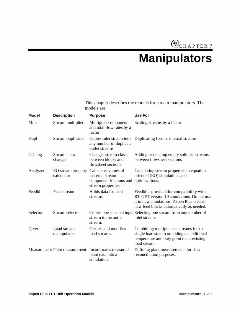
Aspen Plus 11.1 Unit Operation Models Manipulators • 7-1
C H A P T E R 7
Manipulators
This chapter describes the models for stream manipulators. Themodels are:
Model Description Purpose Use For
Mult Stream multiplier Multiplies componentand total flow rates by afactor
Scaling streams by a factor
Dupl Stream duplicator Copies inlet stream intoany number of duplicateoutlet streams
Duplicating feed or internal streams
ClChng Stream classchanger
Changes stream classbetween blocks andflowsheet sections
Adding or deleting empty solid substreamsbetween flowsheet sections
Analyzer EO stream propertycalculator
Calculates values ofmaterial streamcomponent fractions andstream properties.
Calculating stream properties in equation-oriented (EO) simulations andoptimizations.
Feedbl Feed stream Holds data for feedstreams.
Feedbl is provided for compatibility withRT-OPT version 10 simulations. Do not useit in new simulations. Aspen Plus createsnew feed blocks automatically as needed.
Selector Stream selector Copies one selected inputstream to the outletstream.
Selecting one stream from any number ofinlet streams.
Qtvec Load streammanipulator
Creates and modifiesload streams.
Combining multiple heat streams into asingle load stream or adding an additionaltemperature and duty point to an existingload stream.
Measurement Plant measurement Incorporates measuredplant data into asimulation.
Defining plant measurements for datareconciliation purposes.
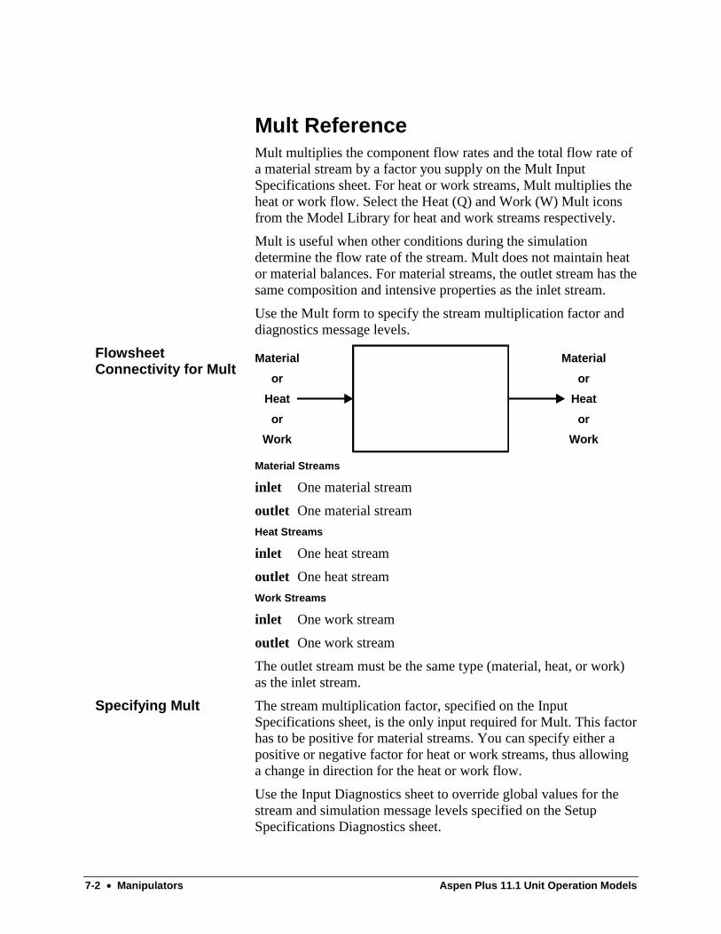
7-2 • Manipulators Aspen Plus 11.1 Unit Operation Models
Mult ReferenceMult multiplies the component flow rates and the total flow rate ofa material stream by a factor you supply on the Mult InputSpecifications sheet. For heat or work streams, Mult multiplies theheat or work flow. Select the Heat (Q) and Work (W) Mult iconsfrom the Model Library for heat and work streams respectively.
Mult is useful when other conditions during the simulationdetermine the flow rate of the stream. Mult does not maintain heator material balances. For material streams, the outlet stream has thesame composition and intensive properties as the inlet stream.
Use the Mult form to specify the stream multiplication factor anddiagnostics message levels.
Material
or
Heat
or
Work
Material
or
Heat
or
Work
Material Streams
inlet One material stream
outlet One material stream
Heat Streams
inlet One heat stream
outlet One heat stream
Work Streams
inlet One work stream
outlet One work stream
The outlet stream must be the same type (material, heat, or work)as the inlet stream.
The stream multiplication factor, specified on the InputSpecifications sheet, is the only input required for Mult. This factorhas to be positive for material streams. You can specify either apositive or negative factor for heat or work streams, thus allowinga change in direction for the heat or work flow.
Use the Input Diagnostics sheet to override global values for thestream and simulation message levels specified on the SetupSpecifications Diagnostics sheet.
FlowsheetConnectivity for Mult
Specifying Mult

Aspen Plus 11.1 Unit Operation Models Manipulators • 7-3
This model has no dynamic features. For material streammultipliers the pressure of each outlet stream is equal to thepressure of the inlet stream. The flow rate of each outlet stream isequal to the flow rate of the inlet stream multiplied by the factor asspecified in the steady-state simulation.
All features of Mult are available in the EO formulation, except thefeatures which are globally unsupported.
EO Usage Notes forMult

7-4 • Manipulators Aspen Plus 11.1 Unit Operation Models
Dupl ReferenceDupl copies an inlet stream (material, heat, or work) to any numberof duplicate outlet streams. It is useful for simultaneouslyprocessing a stream in different types of units. Select the Heat (Q)and Work (W) Dupl icons from the Model Library for heat andwork streams respectively. Dupl does not maintain heat or materialbalances.
Use the Dupl form to specify diagnostics message levels.
Material Material(any number)
Flowsheet for Duplicating Material Streams
Material Streams
inlet One material stream
outlet At least one material stream, which is a copy of the inletstream
Heat Heat(any number)
Flowsheet for Duplicating Heat Streams
Heat Streams
inlet One heat stream
outlet At least one heat stream, which is a copy of the inlet stream
Work Work(any number)
Flowsheet for Duplicating Work Streams
FlowsheetConnectivity for Dupl
Aspen Plus 11.1 Unit Operation Models Manipulators • 7-5
Work Streams
inlet One work stream
outlet At least one work stream, which is a copy of the inletstream
Dupl requires no input parameters. Use the Input Diagnostics sheetto override global values for the stream and simulation messagelevels specified on the Setup Specifications Diagnostics sheet.
This model has no dynamic features. For material streamduplicators the pressure of each outlet stream is equal to thepressure of the inlet stream. The flow rate of each outlet stream isequal to the flow rate of the inlet stream.
All features of Dupl are available in the EO formulation, except thefeatures which are globally unsupported.
Specifying Dupl
EO Usage Notes forDupl
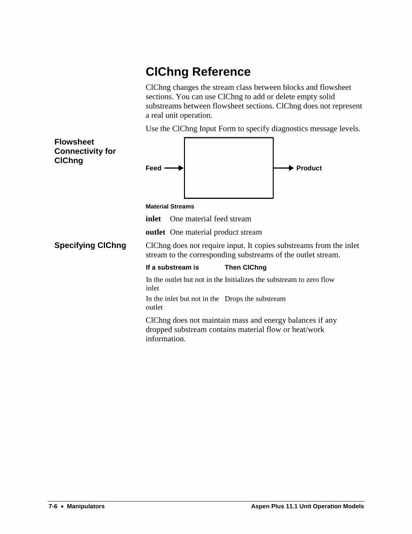
7-6 • Manipulators Aspen Plus 11.1 Unit Operation Models
ClChng ReferenceClChng changes the stream class between blocks and flowsheetsections. You can use ClChng to add or delete empty solidsubstreams between flowsheet sections. ClChng does not representa real unit operation.
Use the ClChng Input Form to specify diagnostics message levels.
Feed Product
Material Streams
inlet One material feed stream
outlet One material product stream
ClChng does not require input. It copies substreams from the inletstream to the corresponding substreams of the outlet stream.
If a substream is Then ClChng
In the outlet but not in theinlet
Initializes the substream to zero flow
In the inlet but not in theoutlet
Drops the substream
ClChng does not maintain mass and energy balances if anydropped substream contains material flow or heat/workinformation.
FlowsheetConnectivity forClChng
Specifying ClChng

Aspen Plus 11.1 Unit Operation Models Manipulators • 7-7
Analyzer ReferenceThe Analyzer block is a mole flow based model that allows you tocalculate values of material stream component fractions and streamproperties for use in the equation-oriented (EO) simulation andoptimization phases of a flowsheet. You can specify one inlet andone outlet material stream, or specify a stream to analyze on theInput form.
Analyzer performs selected analyses on a connected or referencedstream.You refer an existing stream in the flowsheet or specify theconnectivity by identifying an inlet and an outlet stream.
This model calculates requested stream properties at specifiedconditions. The default conditions are the same as the inlet orreferenced stream conditions. You can also specify a temperatureor vapor fraction, in addition to a pressure. In cases where inlet andoutlet streams are given, the outlet stream is a copy of the inletstream.
When using sequential-modular (SM) strategy to solve theproblem, Analyzer has no effect on the stream.
Use the following forms to enter specifications and view results forAnalyzer:
Use this form To do this
Input Specify the Analyzer conditions and referencedstream specifications
Prop Set Specify the property specifications andperturbation data
Block Options Override global values for physical properties,simulation options, diagnostic message levels,EO options, EO variable/vector, and reportoptions for this block
Results View the Analyzer results
EO Variables Specify equation-oriented variable attributechanges for this block, for the current run only
EO Input Specify the equation-oriented variables for thisblock
Spec Groups Specify the specification groups for this block
Ports Specify the EO variables collected to form portsfor this block

7-8 • Manipulators Aspen Plus 11.1 Unit Operation Models
Material (optional)Material (optional)
Material Streams
inlet One inlet material stream (optional)
outlet One outlet material stream (optional)
If Analyzer is not connected to streams, you must specify a streamto analyze on the Input form.
Specify a material stream for Analyzer to analyze by eitherconnecting inlet and outlet material streams to the analyzer blockon the flowsheet or specifying a stream on the Input Specificationssheet. Also on the Input Specifications sheet, you can specifyconditions for the analysis.
Each property you want Analyzer to calculate must be specified ina property set on the top-level Properties Prop-Sets form. Specifyproperties for Analyzer to calculate by choosing these property setson the Analyzer Prop-Set form.
All features of Analyzer are available in the EO formulation,except the features which are globally unsupported.
FlowsheetConnectivity forAnalyzer
Specifying Analyzer
EO Usage Notes forAnalyzer

Aspen Plus 11.1 Unit Operation Models Manipulators • 7-9
Feedbl ReferenceUse Feedbl to maintain compatibility with Feedbl blocks in RT-OPT version 10.0 projects. If you are creating a new simulation inAspen Plus, do not use Feedbl. Aspen Plus automatically createsthe necessary feed specifications.
Feedbl is a mole-flow model which is used to define material feedstreams for the RT-Opt flowsheet. Containing one inlet and oneoutlet material stream, it calculates stream flows, composition, andproperties.
Feedbl includes an extra equation to compute the total molar flowfor the inlet stream. This ensures that the inlet stream componentand total molar flows are consistent. When using sequential-modular (SM) strategy to solve the problem, Feedbl has no effecton the stream, except for an optional pressure drop.
Use the following forms to enter specifications and view results forFeedbl:
Use this form To do this
Input Specify the Feedbl conditions and referencedstream specifications
Prop Set Specify the property specifications andperturbation data
Block Options Override global values for physical properties,simulation options, diagnostic message levels,EO options, EO variable/vector, and reportoptions for this block
Results View the results for this block
EO Variables Specify equation-oriented variable attributechanges for this block, for the current run only
EO Input Specify the equation-oriented variables for thisblock
Spec Groups Specify the specification groups for this block
Ports Specify the EO variables collected to form portsfor this block
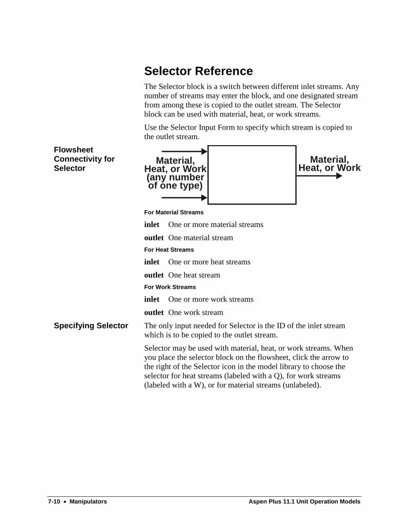
7-10 • Manipulators Aspen Plus 11.1 Unit Operation Models
Selector ReferenceThe Selector block is a switch between different inlet streams. Anynumber of streams may enter the block, and one designated streamfrom among these is copied to the outlet stream. The Selectorblock can be used with material, heat, or work streams.
Use the Selector Input Form to specify which stream is copied tothe outlet stream.
Material,Heat, or Work(any numberof one type)
Material,Heat, or Work
For Material Streams
inlet One or more material streams
outlet One material stream
For Heat Streams
inlet One or more heat streams
outlet One heat stream
For Work Streams
inlet One or more work streams
outlet One work stream
The only input needed for Selector is the ID of the inlet streamwhich is to be copied to the outlet stream.
Selector may be used with material, heat, or work streams. Whenyou place the selector block on the flowsheet, click the arrow tothe right of the Selector icon in the model library to choose theselector for heat streams (labeled with a Q), for work streams(labeled with a W), or for material streams (unlabeled).
FlowsheetConnectivity forSelector
Specifying Selector
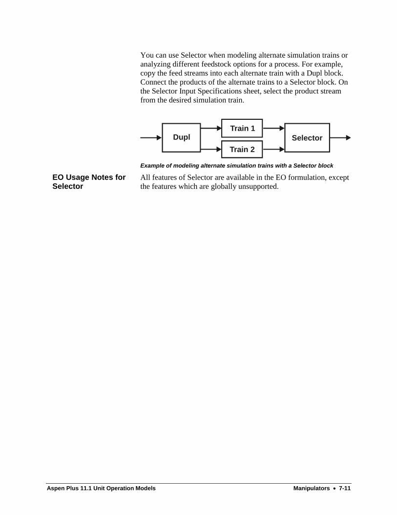
Aspen Plus 11.1 Unit Operation Models Manipulators • 7-11
You can use Selector when modeling alternate simulation trains oranalyzing different feedstock options for a process. For example,copy the feed streams into each alternate train with a Dupl block.Connect the products of the alternate trains to a Selector block. Onthe Selector Input Specifications sheet, select the product streamfrom the desired simulation train.
SelectorDuplTrain 1
Train 2
Example of modeling alternate simulation trains with a Selector block
All features of Selector are available in the EO formulation, exceptthe features which are globally unsupported.
EO Usage Notes forSelector
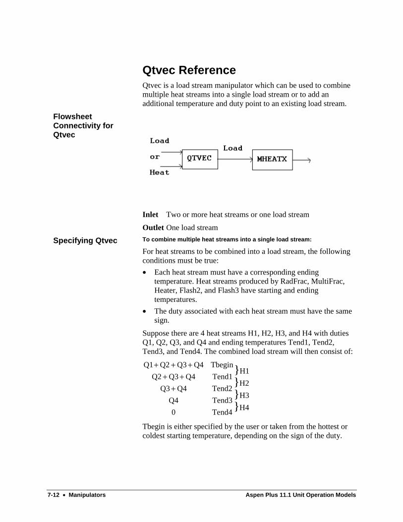
7-12 • Manipulators Aspen Plus 11.1 Unit Operation Models
Qtvec ReferenceQtvec is a load stream manipulator which can be used to combinemultiple heat streams into a single load stream or to add anadditional temperature and duty point to an existing load stream.
Inlet Two or more heat streams or one load stream
Outlet One load stream
To combine multiple heat streams into a single load stream:
For heat streams to be combined into a load stream, the followingconditions must be true:
• Each heat stream must have a corresponding endingtemperature. Heat streams produced by RadFrac, MultiFrac,Heater, Flash2, and Flash3 have starting and endingtemperatures.
• The duty associated with each heat stream must have the samesign.
Suppose there are 4 heat streams H1, H2, H3, and H4 with dutiesQ1, Q2, Q3, and Q4 and ending temperatures Tend1, Tend2,Tend3, and Tend4. The combined load stream will then consist of:
H4
H3
H2
H1
Tend40
Tend3Q4
Tend2Q4Q3
Tend1Q4Q3Q2
TbeginQ4Q3Q2Q1
}}}}
+++
+++
Tbegin is either specified by the user or taken from the hottest orcoldest starting temperature, depending on the sign of the duty.
FlowsheetConnectivity forQtvec
Specifying Qtvec
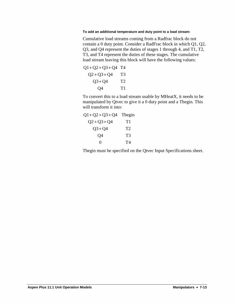
Aspen Plus 11.1 Unit Operation Models Manipulators • 7-13
To add an additional temperature and duty point to a load stream:
Cumulative load streams coming from a Radfrac block do notcontain a 0 duty point. Consider a RadFrac block in which Q1, Q2,Q3, and Q4 represent the duties of stages 1 through 4, and T1, T2,T3, and T4 represent the duties of these stages. The cumulativeload stream leaving this block will have the following values:
T1
T2
T3
T4
Q4
Q4Q3
Q4Q3Q2
Q4Q3Q2Q1
+++
+++
To convert this to a load stream usable by MHeatX, it needs to bemanipulated by Qtvec to give it a 0 duty point and a Tbegin. Thiswill transform it into:
4T0
T3Q4
T2Q4Q3
T1Q4Q3Q2
TbeginQ4Q3Q2Q1
+++
+++
Tbegin must be specified on the Qtvec Input Specifications sheet.

7-14 • Manipulators Aspen Plus 11.1 Unit Operation Models
Measurement ReferenceThe measurement model is used to define plant measurements fordata reconciliation purposes. It provides a:
• Way of relating plant measurements to model predictions
• Mechanism for entering values for plant measurements
It also provides a convenient method for supplying a datareconciliation objective, by allowing you to specify the objectivefunction in terms of measurement offsets and standard deviations.
Use the following forms to enter specifications and view results forMeasurement:
Use this form To do this
Input Specify the measurement and flowsheetvariables for this block.
Results View the Measurement results
EO Variables Specify equation-oriented variable attributechanges related to this block for the currentrun only
EO Input Specify the equation-oriented variables forthis block

Aspen Plus 11.1 Unit Operation Models Solids • 8-1
C H A P T E R 8
Solids
This chapter describes the unit operation models for solidsprocessing such as crystallizers, solid crushers and separators, gas-solid separators, liquid-solid separators, and solids washers. Themodels are:
Model Description Purpose Use For
Crystallizer Crystallizer Produces crystals from solution based onsolubility
Mixed suspension, mixed productremoval (MSMPR) crystallizer
Crusher Solids crusher Breaks solid particles to reduce particlesize
Wet and dry crushers, primary andsecondary crushers
Screen Solidsseparator
Separates solid particles based onparticle size
Upper and lower dry and wetscreens
FabFl Fabric filter Separates solids from gas using fabricfilter baghouses
Rating and sizing baghouses
Cyclone Cycloneseparator
Separates solids from gas using gasvortex in a cyclone
Rating and sizing cyclones
VScrub Venturiscrubber
Separates solids from gas by directcontact with an atomized liquid
Rating and sizing venturi scrubbers
ESP Electrostaticprecipitator
Separates solids from gas using anelectric charge between two plates
Rating and sizing dry electrostaticprecipitators
HyCyc Hydrocyclone Separates solids from liquid using liquidvortex in a hydrocyclone
Rating or sizing hydrocyclones
CFuge Centrifugefilter
Separates solids from liquid using arotating basket
Rating or sizing centrifuges
Filter Rotary vacuumfilter
Separates solids from liquid using acontinuous rotary vacuum filter
Rating or sizing rotary vacuumfilters
SWash Single-stagesolids washer
Models recovery of dissolvedcomponents from an entrained liquid of asolids stream using a washing liquid
Single -stage solids washer
CCD Counter-currentdecanter
Models multi-stage recovery of dissolvedcomponents from an entrained liquid of asolids stream using a washing liquid
Multi-stage solids washers

8-2 • Solids Aspen Plus 11.1 Unit Operation Models
This chapter is organized into the following sections:
Section Models
Crystallizer Crystallizer
Crushers and Screens Crusher, Screen
Gas-Solid Separators FabFl, Cyclone, VScrub, ESP
Liquid-Solid Separators HyCyc, CFuge, Filter
Solids Washers SWash, CCD
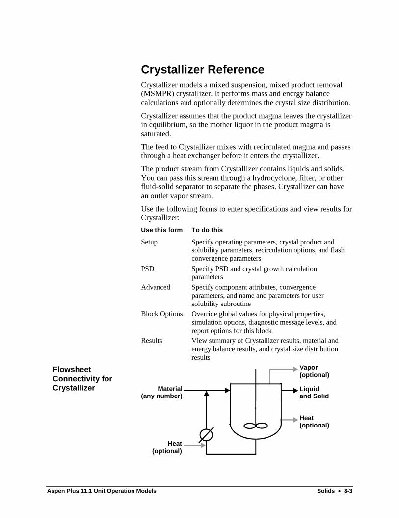
Aspen Plus 11.1 Unit Operation Models Solids • 8-3
Crystallizer ReferenceCrystallizer models a mixed suspension, mixed product removal(MSMPR) crystallizer. It performs mass and energy balancecalculations and optionally determines the crystal size distribution.
Crystallizer assumes that the product magma leaves the crystallizerin equilibrium, so the mother liquor in the product magma issaturated.
The feed to Crystallizer mixes with recirculated magma and passesthrough a heat exchanger before it enters the crystallizer.
The product stream from Crystallizer contains liquids and solids.You can pass this stream through a hydrocyclone, filter, or otherfluid-solid separator to separate the phases. Crystallizer can havean outlet vapor stream.
Use the following forms to enter specifications and view results forCrystallizer:
Use this form To do this
Setup Specify operating parameters, crystal product andsolubility parameters, recirculation options, and flashconvergence parameters
PSD Specify PSD and crystal growth calculationparameters
Advanced Specify component attributes, convergenceparameters, and name and parameters for usersolubility subroutine
Block Options Override global values for physical properties,simulation options, diagnostic message levels, andreport options for this block
Results View summary of Crystallizer results, material andenergy balance results, and crystal size distributionresults
Material(any number)
Heat(optional)
Vapor(optional)
Heat(optional)
Liquidand Solid
FlowsheetConnectivity forCrystallizer
8-4 • Solids Aspen Plus 11.1 Unit Operation Models
Material Streams
inlet At least one material stream
outlet One material stream for liquid and solidOne optional vapor stream
The outlet material stream should normally have at least one solidsubstream for the crystals formed. If you select Calculate PSDfrom Growth Kinetics or User-Specified Values on the PSD PSDsheet, each substream must have a particle size distribution (PSD)attribute.
If electrolyte salts are formed based on electrolyte chemistrycalculations, a solid substream is not required when you selectCopy from Inlet Stream on the PSD PSD sheet.
If you do not use the vapor outlet stream, vapor products will beplaced in the liquid/solid product stream.
Heat Streams
inlet Any number of optional inlet heat streams
outlet One optional outlet heat stream
If you give only one specification on the Setup Specifications sheet(temperature or pressure), Crystallizer uses the sum of the inletheat streams as a duty specification. Otherwise, Crystallizer usesthe inlet heat streams only to calculate the net heat duty. The netheat duty is the sum of the inlet heat streams minus the actual(calculated) heat duty.
You can use an optional outlet heat stream for the net heat duty.
Crystallizer calculates crystal product flow rate and/or vapor flow,based on solubility data you supply. Or you can specify thechemistry for electrolyte systems instead of specifying solubilitydata.
You must specify two of the following:
• Crystallizer temperature
• Pressure or pressure drop
• Heat duty for the heat exchanger
• Crystal product flow rate
• Vapor flow
SpecifyingCrystallizer
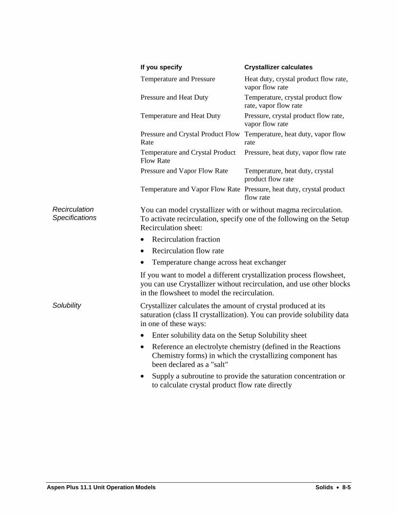
Aspen Plus 11.1 Unit Operation Models Solids • 8-5
If you specify Crystallizer calculates
Temperature and Pressure Heat duty, crystal product flow rate,vapor flow rate
Pressure and Heat Duty Temperature, crystal product flowrate, vapor flow rate
Temperature and Heat Duty Pressure, crystal product flow rate,vapor flow rate
Pressure and Crystal Product FlowRate
Temperature, heat duty, vapor flowrate
Temperature and Crystal ProductFlow Rate
Pressure, heat duty, vapor flow rate
Pressure and Vapor Flow Rate Temperature, heat duty, crystalproduct flow rate
Temperature and Vapor Flow Rate Pressure, heat duty, crystal productflow rate
You can model crystallizer with or without magma recirculation.To activate recirculation, specify one of the following on the SetupRecirculation sheet:
• Recirculation fraction
• Recirculation flow rate
• Temperature change across heat exchanger
If you want to model a different crystallization process flowsheet,you can use Crystallizer without recirculation, and use other blocksin the flowsheet to model the recirculation.
Crystallizer calculates the amount of crystal produced at itssaturation (class II crystallization). You can provide solubility datain one of these ways:
• Enter solubility data on the Setup Solubility sheet
• Reference an electrolyte chemistry (defined in the ReactionsChemistry forms) in which the crystallizing component hasbeen declared as a "salt"
• Supply a subroutine to provide the saturation concentration orto calculate crystal product flow rate directly
RecirculationSpecifications
Solubility
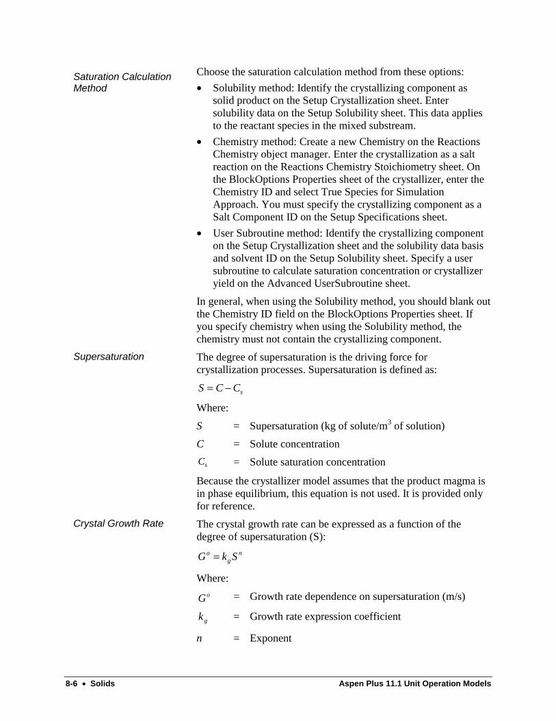
8-6 • Solids Aspen Plus 11.1 Unit Operation Models
Choose the saturation calculation method from these options:
• Solubility method: Identify the crystallizing component assolid product on the Setup Crystallization sheet. Entersolubility data on the Setup Solubility sheet. This data appliesto the reactant species in the mixed substream.
• Chemistry method: Create a new Chemistry on the ReactionsChemistry object manager. Enter the crystallization as a saltreaction on the Reactions Chemistry Stoichiometry sheet. Onthe BlockOptions Properties sheet of the crystallizer, enter theChemistry ID and select True Species for SimulationApproach. You must specify the crystallizing component as aSalt Component ID on the Setup Specifications sheet.
• User Subroutine method: Identify the crystallizing componenton the Setup Crystallization sheet and the solubility data basisand solvent ID on the Setup Solubility sheet. Specify a usersubroutine to calculate saturation concentration or crystallizeryield on the Advanced UserSubroutine sheet.
In general, when using the Solubility method, you should blank outthe Chemistry ID field on the BlockOptions Properties sheet. Ifyou specify chemistry when using the Solubility method, thechemistry must not contain the crystallizing component.
The degree of supersaturation is the driving force forcrystallization processes. Supersaturation is defined as:
S C Cs= −
Where:
S = Supersaturation (kg of solute/m3 of solution)
C = Solute concentration
Cs = Solute saturation concentration
Because the crystallizer model assumes that the product magma isin phase equilibrium, this equation is not used. It is provided onlyfor reference.
The crystal growth rate can be expressed as a function of thedegree of supersaturation (S):
ng
o SkG =
Where:
Go = Growth rate dependence on supersaturation (m/s)
kg = Growth rate expression coefficient
n = Exponent
Saturation CalculationMethod
Supersaturation
Crystal Growth Rate
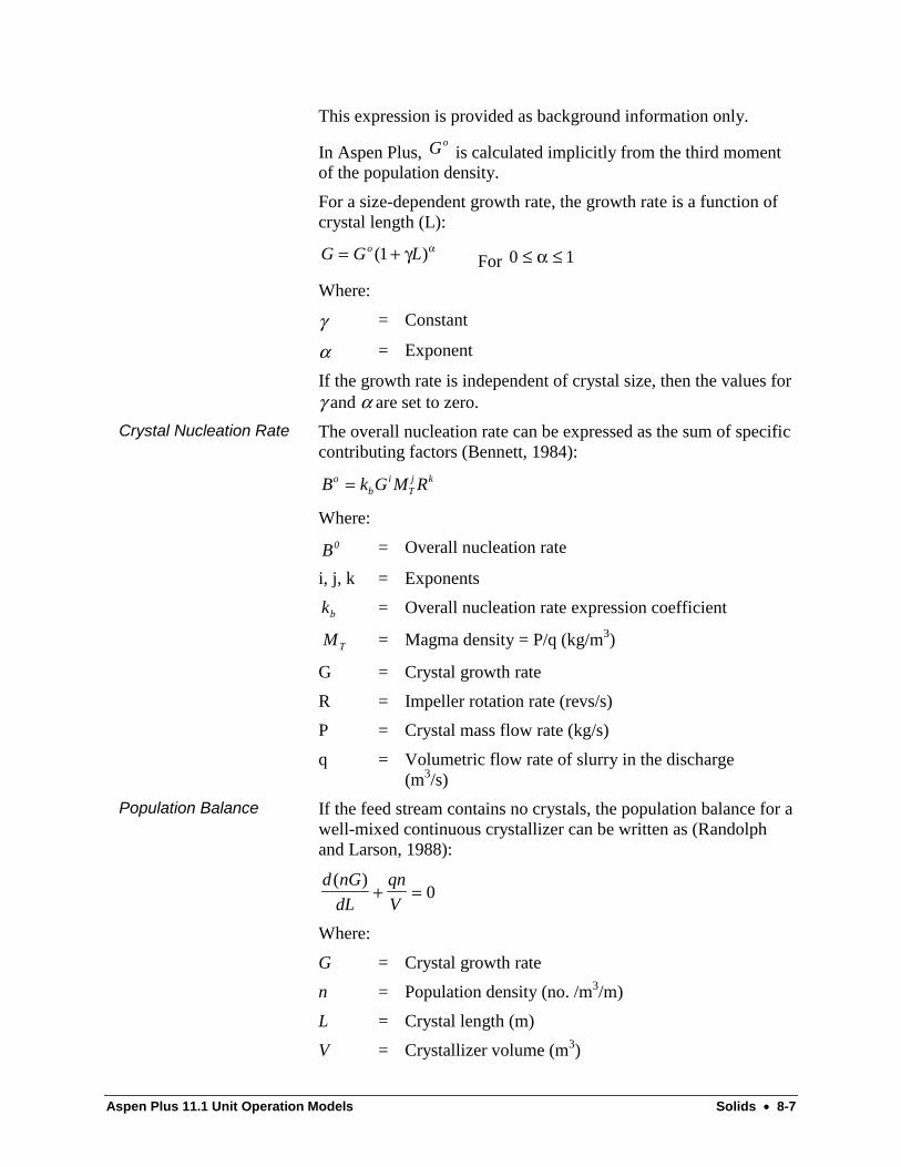
Aspen Plus 11.1 Unit Operation Models Solids • 8-7
This expression is provided as background information only.
In Aspen Plus, Go is calculated implicitly from the third moment
of the population density.
For a size-dependent growth rate, the growth rate is a function ofcrystal length (L):
G G Lo= +( )1 γ αFor 0 1≤ ≤α
Where:
γ = Constant
α = Exponent
If the growth rate is independent of crystal size, then the values forγ and α are set to zero.
The overall nucleation rate can be expressed as the sum of specificcontributing factors (Bennett, 1984):
B k G M Rob
iTj k=
Where:
B0 = Overall nucleation rate
i, j, k = Exponents
kb = Overall nucleation rate expression coefficient
MT = Magma density = P/q (kg/m3)
G = Crystal growth rate
R = Impeller rotation rate (revs/s)
P = Crystal mass flow rate (kg/s)
q = Volumetric flow rate of slurry in the discharge(m3/s)
If the feed stream contains no crystals, the population balance for awell-mixed continuous crystallizer can be written as (Randolphand Larson, 1988):
d nG
dL
qn
V
( )+ = 0
Where:
G = Crystal growth rate
n = Population density (no. /m3/m)
L = Crystal length (m)
V = Crystallizer volume (m3)
Crystal Nucleation Rate
Population Balance

8-8 • Solids Aspen Plus 11.1 Unit Operation Models
q = Volumetric flow rate of slurry in the discharge(m3/s)
The boundary condition is n no= at L = 0, where n B Go o= / isthe population density of nuclei. For a constant crystal growth rate,the population density is:
n L nL
Go( ) = −
expτ
where τ = V / q is the crystal residence time.
Aspen Plus calculates the crystal size distribution statistics onceyou select the Calculate PSD from Growth Kinetics option on thePSD PSD sheet.
Properties of the distribution may be evaluated from the momentequations. The j-th moment of the particle size distribution isdefined as:
m L n L dLjj=
∞
∫0 ( )
The system reports several crystal size distribution statistics,measured on a volume or mass basis, including:
• Mean size
• Standard deviation
• Skewness
• The coefficient of variation (expressed as a percentage)
The mean size is the mass-weighted average crystal size, asdetermined by the ratio of the fourth moment to the third moment,as follows:
Lm
m= 4
3
The skewness of a symmetric size distribution about the mean iszero. Negative values of skewness indicate the distribution isskewed toward the presence of small crystals. Positive values ofskewness indicate the crystal distribution contains an excess oflarge crystals.
Skewness is defined as
∑ −f ( )
( )
x mean
standard deviation
3
3
.
The system uses the coefficient of variation to calculate variationrelated to the cumulative volume (or mass) distribution.
PSD Statistics

Aspen Plus 11.1 Unit Operation Models Solids • 8-9
Coeff Var(%)− =−
10084 16
2 50
pd pd
pd
@(. ) @(. )
@(. )
where pd@ (x) is the particle diameter corresponding to fraction xof the cumulative volume (or mass) distribution. The fraction canbe entered as the Fractional Coefficient on the PSD CrystalGrowthsheet; otherwise, it defaults to .16.
The magma density, defined as total mass of crystals per unitvolume of slurry, can be obtained from the third moment:
dLLnLkM vcT )(3
0∫∞
= ρ
Where:
cρ = Density of crystal (kg/m3)
vk = Volume shape factor of the crystal
Since:
n L nL
Go( ) = −
expτ ,
nB
Go
o
o=,
and B k G M Rob
iTj k=
these equations can be substituted into the third moment ofpopulation density, yielding:
M k L kG
GM R
L
GdLT c v b
i
o Tj k=
−
∞
∫ρτ
3
0exp
where G G Lo= +( )1 γ α.
Because L is made discrete by the increments of the particle size
distribution, the equations can be solved for Go.
Bennett, R.C. "Crystallization from Solution", in Perry’s ChemicalEngineers’ Handbook, 6th Ed., pp. 19.24-19.40, McGraw-Hill,1984.
Randolph, A.D. and Larson, M.A., Theory of ParticulateProcesses, 2nd Ed., Academic Press, 1988.
Calculating PSD
References
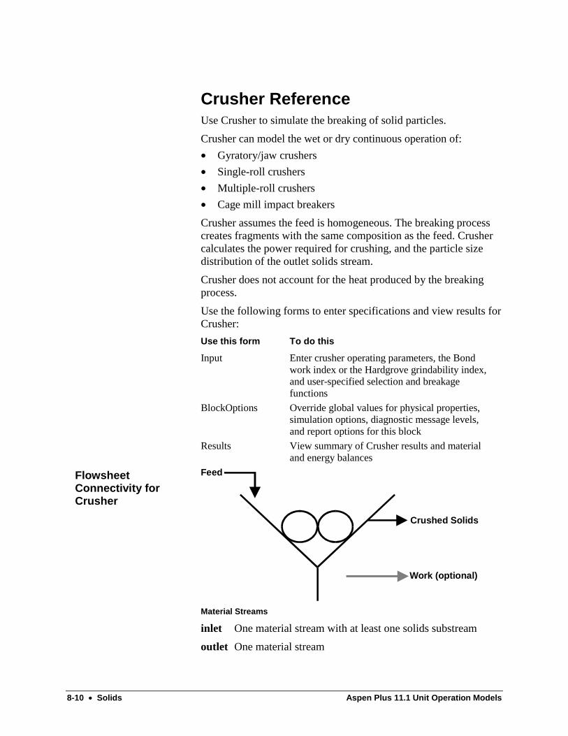
8-10 • Solids Aspen Plus 11.1 Unit Operation Models
Crusher ReferenceUse Crusher to simulate the breaking of solid particles.
Crusher can model the wet or dry continuous operation of:
• Gyratory/jaw crushers
• Single-roll crushers
• Multiple-roll crushers
• Cage mill impact breakers
Crusher assumes the feed is homogeneous. The breaking processcreates fragments with the same composition as the feed. Crushercalculates the power required for crushing, and the particle sizedistribution of the outlet solids stream.
Crusher does not account for the heat produced by the breakingprocess.
Use the following forms to enter specifications and view results forCrusher:
Use this form To do this
Input Enter crusher operating parameters, the Bondwork index or the Hardgrove grindability index,and user-specified selection and breakagefunctions
BlockOptions Override global values for physical properties,simulation options, diagnostic message levels,and report options for this block
Results View summary of Crusher results and materialand energy balances
Feed
Crushed Solids
Work (optional)
Material Streams
inlet One material stream with at least one solids substream
outlet One material stream
FlowsheetConnectivity forCrusher
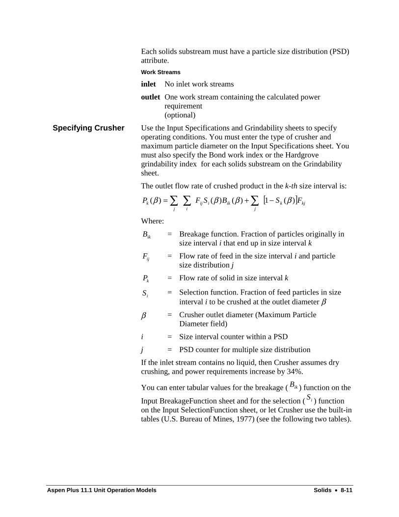
Aspen Plus 11.1 Unit Operation Models Solids • 8-11
Each solids substream must have a particle size distribution (PSD)attribute.
Work Streams
inlet No inlet work streams
outlet One work stream containing the calculated powerrequirement(optional)
Use the Input Specifications and Grindability sheets to specifyoperating conditions. You must enter the type of crusher andmaximum particle diameter on the Input Specifications sheet. Youmust also specify the Bond work index or the Hardgrovegrindability index for each solids substream on the Grindabilitysheet.
The outlet flow rate of crushed product in the k-th size interval is:
[ ] kjkj
ikiijij
k FSBSFP )(1)()()( ββββ −+= ∑∑∑Where:
Bik = Breakage function. Fraction of particles originally insize interval i that end up in size interval k
Fij = Flow rate of feed in the size interval i and particlesize distribution j
Pk = Flow rate of solid in size interval k
iS = Selection function. Fraction of feed particles in sizeinterval i to be crushed at the outlet diameter β
β = Crusher outlet diameter (Maximum ParticleDiameter field)
i = Size interval counter within a PSD
j = PSD counter for multiple size distribution
If the inlet stream contains no liquid, then Crusher assumes drycrushing, and power requirements increase by 34%.
You can enter tabular values for the breakage ( Bik ) function on the
Input BreakageFunction sheet and for the selection ( iS ) functionon the Input SelectionFunction sheet, or let Crusher use the built-intables (U.S. Bureau of Mines, 1977) (see the following two tables).
Specifying Crusher

8-12 • Solids Aspen Plus 11.1 Unit Operation Models
Breakage Function Correlations Bik ( )β
Ratio of productsize to feed size
Feed size/solids outlet diameter >1.7 Feed size/solids outletdiameter <1.7
Multiple rollcrusher
Gyratory/jawcrusher
Single rollcrusher
Cage millcrusher
All crushers
1.0 1.0 1.0 1.0 1.0 1.0
0.8308 0.95 0.95 0.96 0.84 0.8972
0.5882 0.85 0.85 0.79 0.50 0.7035
0.4176 0.65 0.70 0.45 0.32 0.54
0.2065 0.35 0.35 0.20 0.15 0.2952
0.1041 0.22 0.20 0.10 0.052 0.1564
0.0522 0.14 0.19 0.05 0.019 0.0805
0.0368 0.11 0.17 0.03 0.011 0.0572
0.026 0.09 0.12 0.02 0.0066 0.0406
0.0131 0.03 0.08 0.0 0.002 0.0206
0.0 0.0 0.0 0.0 0.0 0.0
Selection Function Correlations, Si ( )β
Ratio of feed size tooutlet diameter
Primary crusher Secondary crusher
0.95 0.5695 0.7693
0.9 0.3817 0.6962
0.8 0.1716 0.5695
0.7 0.0771 0.4667
0.6 0.0347 0.3817
0.5 0.0156 0.3128
0.4 0.007 0.256
0.3 0.00315 0.2096
0.2 0.00145 0.1716
0.1 0.0006 0.1405
0.05 0.00043 0.1271
0.001 0.00026 0.1153
0.0001 0.00026 0.1148
If the ratio of feed size to outlet diameter is greater than 1.0, thenSi ( ) .β = 0 85 .
Crushing operations are usually performed in stages. The reductionratio is the ratio of the maximum diameter of feed particles toproduct particles. The reduction ratio in crushers ranges from 3 to6 per stage. Feed particles are fed to the primary crushers. Outletparticles from the primary crushers are reduced further by thesecondary crushers.
Primary and SecondaryCrushers
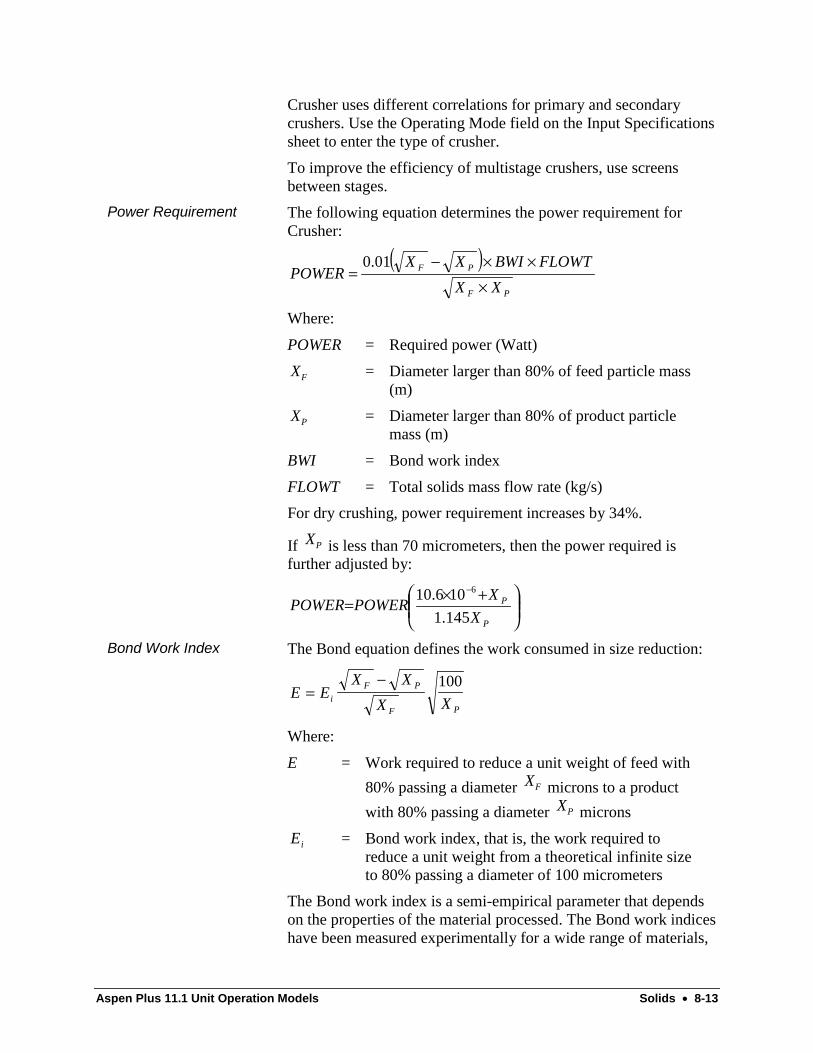
Aspen Plus 11.1 Unit Operation Models Solids • 8-13
Crusher uses different correlations for primary and secondarycrushers. Use the Operating Mode field on the Input Specificationssheet to enter the type of crusher.
To improve the efficiency of multistage crushers, use screensbetween stages.
The following equation determines the power requirement forCrusher:
( )PF
PF
XX
FLOWTBWIXXPOWER
×××−
=01.0
Where:
POWER = Required power (Watt)
XF = Diameter larger than 80% of feed particle mass(m)
XP = Diameter larger than 80% of product particlemass (m)
BWI = Bond work index
FLOWT = Total solids mass flow rate (kg/s)
For dry crushing, power requirement increases by 34%.
If XP is less than 70 micrometers, then the power required isfurther adjusted by:
+×=
−
P
P
X
XPOWERPOWER
145.1
106.10 6
The Bond equation defines the work consumed in size reduction:
E EX X
X Xi
F P
F P
=− 100
Where:
E = Work required to reduce a unit weight of feed with
80% passing a diameter XF microns to a product
with 80% passing a diameter XP microns
Ei = Bond work index, that is, the work required toreduce a unit weight from a theoretical infinite sizeto 80% passing a diameter of 100 micrometers
The Bond work index is a semi-empirical parameter that dependson the properties of the material processed. The Bond work indiceshave been measured experimentally for a wide range of materials,
Power Requirement
Bond Work Index
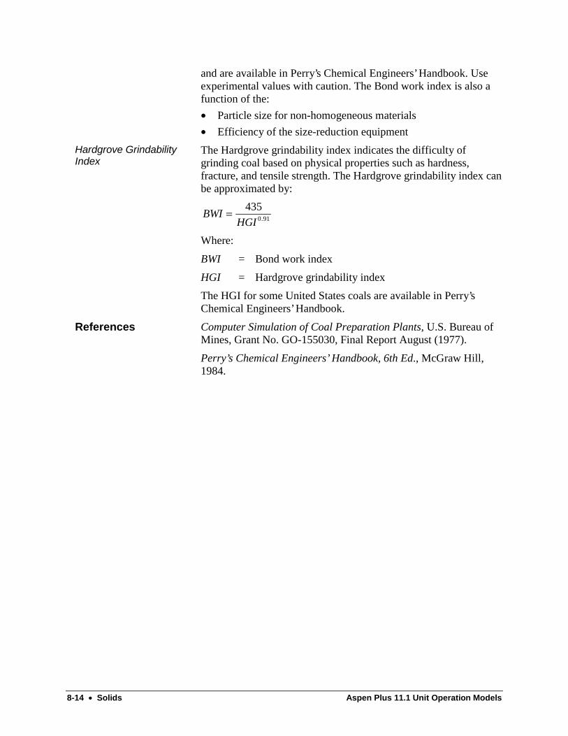
8-14 • Solids Aspen Plus 11.1 Unit Operation Models
and are available in Perry’s Chemical Engineers’ Handbook. Useexperimental values with caution. The Bond work index is also afunction of the:
• Particle size for non-homogeneous materials
• Efficiency of the size-reduction equipment
The Hardgrove grindability index indicates the difficulty ofgrinding coal based on physical properties such as hardness,fracture, and tensile strength. The Hardgrove grindability index canbe approximated by:
BWIHGI
= 4350 91.
Where:
BWI = Bond work index
HGI = Hardgrove grindability index
The HGI for some United States coals are available in Perry’sChemical Engineers’ Handbook.
Computer Simulation of Coal Preparation Plants, U.S. Bureau ofMines, Grant No. GO-155030, Final Report August (1977).
Perry’s Chemical Engineers’ Handbook, 6th Ed., McGraw Hill,1984.
Hardgrove GrindabilityIndex
References

Aspen Plus 11.1 Unit Operation Models Solids • 8-15
Screen ReferenceScreen simulates the separation by screens of a mixture containingvarious sizes of solid particles into particles that have moreuniform sizes than the original mixture. You can use Screen tomodel wet or dry operations and upper or lower level screens.
Screen calculates the separation efficiency of the screen from thesize of screen openings you specify.
Use the following forms to enter specifications and view results forScreen:
Use this form To do this
Input Specify screen parameters, operating conditions,and user-specified screen separation strength andselection functions
Block Options Override global values for physical properties,simulation options, diagnostic message levels,and report options for this block
Results View summary of Screen results and materialand energy balances
Feed
Overflow
Underflow
Material Streams
inlet One material stream with at least one solids substream
outlet One material stream for particles that do not pass throughthe screen (overflow)One material stream for particles that pass through thescreen (underflow)
Each solids substream must have a particle size distributionattribute.
Use the Input Specifications sheet to enter:
• Screen size opening
• Operating level (Upper or Lower)
• Operating mode (Wet or Dry)
• Entrainments
FlowsheetConnectivity forScreen
Specifying Screen

8-16 • Solids Aspen Plus 11.1 Unit Operation Models
You can also use the Input SelectionFunction sheet to enter thefollowing functions:
• Selection function ( Si ) (optional)
• Separation strength (optional)
You can specify the operating level as Upper or Lower. The mostefficient configuration is a multiple-deck screen with a series ofScreen blocks. The inlet stream is fed over the upper level screen.The underflow from the upper level screens is fed over the lowerlevel screens. Screen uses different correlations for upper andlower level screens.
Screen calculates the flow rate of the screen overflow stream as:
F S Fo ii
ijj
= ∑ ∑
Where:
Si = Selection function. The fraction of feed particles insize range i that passes over the screen into theoverflow product
Fij = Flow rate of feed in size range i and particle sizedistribution attribute j
Screen calculates the selection function for a certain size intervalas:
( )[ ]SA d S
for d Si
p o
p o=−
<1
1exp
S for d Si p o= ≥1
Where:
d p = Particle diameter
So = Size of screen opening
A = Separation strength
The default value of the screen separation strength, A, is a functionof the size of the screen opening. Screen has four built-in functions(U.S. Bureau of Mines, 1977) for all possible combinations ofscreen types (see the table, Screen Separation Strength/Screen SizeCorrelation):
• Upper level dry
• Lower level dry
• Upper level wet
• Lower level wet
Upper and Lower LevelScreens
Selection Function andSeparation Strength

Aspen Plus 11.1 Unit Operation Models Solids • 8-17
You can enter your own separation strength value, separationstrength correlation or selection function correlation on the InputSelectionFunction sheet. Screen then uses these selection functionvalues for its mass balance calculation.
Screen Separation Strength/Screen Size Correlation
Size of screenopening (m)
Dry, upperlevel
Dry, lowerlevel
Wet, upperlevel
Wet, lowerlevel
0.457 60 60 60 60
0.152 20 20 20 20
0.038 8 8 9 9
0.0095 8 6 8.5 6.6
0.00635 5 4 5.5 4.5
0.00236 3 2 3.5 2.3
0.00059 0.7 0.7 0.8 0.8
0.00042 0.6 0.6 0.7 0.7
0.000295 0.5 0.5 0.55 0.55
The separation efficiency of the screen is calculated as the ratio ofthe mass flow rate of the underflow to the fraction of the feed flowrate containing particles smaller than the screen openings.
Computer Simulation of Coal Preparation Plants, U.S. Bureau ofMines, Grant No. GO-155030, Final Report August (1977).
Separation Efficiency
Reference

8-18 • Solids Aspen Plus 11.1 Unit Operation Models
FabFl ReferenceFabFl is a gas-solids separator model used to separate an inlet gasstream containing solids into a solids stream and a gas streamcarrying the residual solids. Use FabFl to simulate or designbaghouse units in which solid particles are separated from the inletgas stream. A baghouse consists of a number of cells in whichvertically-mounted cylindrical fabric filter bags operate in parallel.
You can use FabFl to rate or size baghouses.
Use the following forms to enter specifications and view results forFabFl:
Use this form To do this
Input Enter operating conditions, baghousecharacteristics, and separation efficiency
BlockOptions Override global values for physical properties,simulation options, diagnostic message levels,and report options for this block
Results View summary of FabFl results and material andenergy balances
Feed
Gas (overflow)
Solids (underflow)
Material Streams
inlet One material stream with at least one solids substream
outlet One overflow stream for the cleaned gasOne underflow stream for the solids particles
Each solids substream must have a particle size distribution (PSD)attribute. Solids may be entrained in the overflow, based on theseparation efficiency.
Use the Input Specifications sheet to specify operating conditionsand baghouse characteristics.
For these calculations Set Mode= And number of cells is
Rating Simulation Specified
Sizing Design Calculated
FlowsheetConnectivity forFabFl
Specifying FabFl
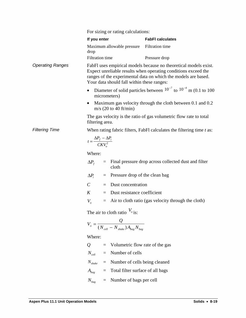
Aspen Plus 11.1 Unit Operation Models Solids • 8-19
For sizing or rating calculations:
If you enter FabFl calculates
Maximum allowable pressuredrop
Filtration time
Filtration time Pressure drop
FabFl uses empirical models because no theoretical models exist.Expect unreliable results when operating conditions exceed theranges of the experimental data on which the models are based.Your data should fall within these ranges:
• Diameter of solid particles between 10 7− to 10 4−
m (0.1 to 100micrometers)
• Maximum gas velocity through the cloth between 0.1 and 0.2m/s (20 to 40 ft/min)
The gas velocity is the ratio of gas volumetric flow rate to totalfiltering area.
When rating fabric filters, FabFl calculates the filtering time t as:
tP P
CKVf i
o
=−∆ ∆
2
Where:
fP∆ = Final pressure drop across collected dust and filtercloth
iP∆ = Pressure drop of the clean bag
C = Dust concentration
K = Dust resistance coefficient
oV = Air to cloth ratio (gas velocity through the cloth)
The air to cloth ratio Vo is:
VQ
N N A Nocell shake bag bag
=−( )
Where:
Q = Volumetric flow rate of the gas
Ncell = Number of cells
Nshake = Number of cells being cleaned
Abag = Total filter surface of all bags
Nbag = Number of bags per cell
Operating Ranges
Filtering Time
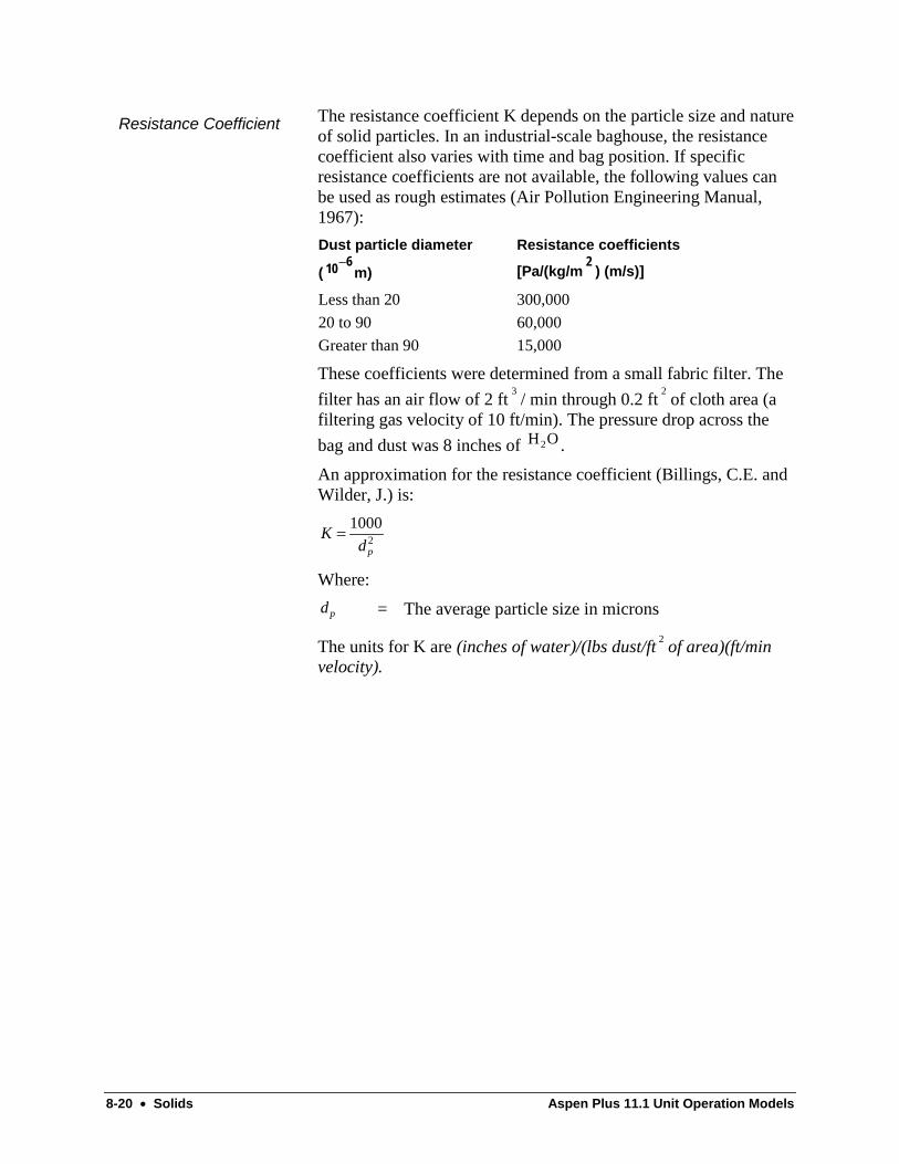
8-20 • Solids Aspen Plus 11.1 Unit Operation Models
The resistance coefficient K depends on the particle size and natureof solid particles. In an industrial-scale baghouse, the resistancecoefficient also varies with time and bag position. If specificresistance coefficients are not available, the following values canbe used as rough estimates (Air Pollution Engineering Manual,1967):
Dust particle diameter
( 10 6−m)
Resistance coefficients
[Pa/(kg/m2
) (m/s)]
Less than 20 300,000
20 to 90 60,000
Greater than 90 15,000
These coefficients were determined from a small fabric filter. The
filter has an air flow of 2 ft3
/ min through 0.2 ft2
of cloth area (afiltering gas velocity of 10 ft/min). The pressure drop across the
bag and dust was 8 inches of H O2 .
An approximation for the resistance coefficient (Billings, C.E. andWilder, J.) is:
Kdp
= 10002
Where:
dp = The average particle size in microns
The units for K are (inches of water)/(lbs dust/ft2
of area)(ft/minvelocity).
Resistance Coefficient

Aspen Plus 11.1 Unit Operation Models Solids • 8-21
The overall separation efficiency of the baghouse is:
ηη
oj i
ij ijS
Total inlet flow rate of solids
flow rate of solids removed from the inlet
total inlet flow rate of solids= =
∑ ∑
Where:
Sij = Flow rate of solid j in size increment i
In FabFl, the separation efficiency is a function of the particlediameter of the solids. For large particles (greater than 10
micrometers in diameter), fractional collection efficiency( )ηi is1.0. For particles smaller than 10 micrometers, efficiencydecreases rapidly.
η iWhen
1.0 ( )d mp av >10 µ
0.0011( )dp av 0.989
1 10µ µm (dp< <)av m
0.495( )dp av 0.495
( )dp av <1µm
You also can enter efficiency as a function of particle sizes on theInput Efficiency sheet to override the built-in correlations.
Air Pollution Engineering Manual, Public Health ServicePublication No. 999-AP-40, pp. 106-135, Washington D.C.,DHEW (1967).
Billings, C.E. and Wilder, J., Handbook of Fabric FilterTechnology, Vol. I, NIIS PB 200648.
Separation Efficiency
References
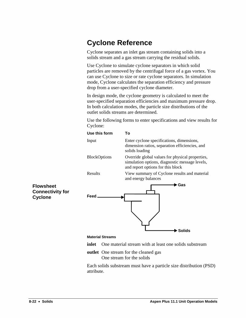
8-22 • Solids Aspen Plus 11.1 Unit Operation Models
Cyclone ReferenceCyclone separates an inlet gas stream containing solids into asolids stream and a gas stream carrying the residual solids.
Use Cyclone to simulate cyclone separators in which solidparticles are removed by the centrifugal force of a gas vortex. Youcan use Cyclone to size or rate cyclone separators. In simulationmode, Cyclone calculates the separation efficiency and pressuredrop from a user-specified cyclone diameter.
In design mode, the cyclone geometry is calculated to meet theuser-specified separation efficiencies and maximum pressure drop.In both calculation modes, the particle size distributions of theoutlet solids streams are determined.
Use the following forms to enter specifications and view results forCyclone:
Use this form To
Input Enter cyclone specifications, dimensions,dimension ratios, separation efficiencies, andsolids loading
BlockOptions Override global values for physical properties,simulation options, diagnostic message levels,and report options for this block
Results View summary of Cyclone results and materialand energy balances
Feed
Gas
Solids
Material Streams
inlet One material stream with at least one solids substream
outlet One stream for the cleaned gasOne stream for the solids
Each solids substream must have a particle size distribution (PSD)attribute.
FlowsheetConnectivity forCyclone

Aspen Plus 11.1 Unit Operation Models Solids • 8-23
Use the Input Specifications sheet to specify the type of cycloneand operating conditions.
Use the Input Dimensions sheet to enter cyclone dimensions, oruse the Input Ratios sheet to enter ratios of cyclone dimensions.
To performthese calculations Specify Cyclone calculates
Rating Simulation modeCyclone DiameterNumber of Cyclones
Separation efficiencyPressure drop
Sizing Design modeSeparation EfficiencyMaximum PressureDrop (optional)Maximum Number ofCyclones (optional)
Cyclone diameterNumber of cyclones
For rating calculations, if you specify Type=User-Specified orUser-Specified Ratios, you can specify cyclone dimensions on theInput Dimensions or Input Ratios sheets.
For design calculations, you must also enter the Maximum Numberof Cyclones in parallel. If either of the following occurs, Cyclonecalculates the number of cyclones in parallel:
• The efficiency of a single cyclone is less than the requiredseparation efficiency.
• The calculated pressure drop exceeds the maximum pressuredrop specified.
The overall separation efficiency is:
ηm
flow rate of solids removed from the inlet
total inlet flow rate of solids=
ηmo i
o
o o
o o o o
C C
C
Q C E
Q C
E
Q C=
−=
−= −1
Where:
Co = Concentration of solids in inlet gas
Ci = Concentration of solids in outlet cleaned gas
Qo = Inlet gas flow rate
E = Outlet emission rate of solids in the cleaned gas
Cyclone attains higher separation efficiencies with particles thatare 5 to 10 microns or greater in diameter. For particles smallerthan 5 microns, Cyclone efficiency decreases. Even with largeparticles, it is difficult to obtain a collection efficiency greater than95%.
Specifying Cyclone
Separation Efficiency

8-24 • Solids Aspen Plus 11.1 Unit Operation Models
If you enter a design efficiency higher than 95%, use either:
• Multi-stage cyclones
• Cyclone as a precleaner, followed by other collectors
You can specify the Efficiency Correlation field on the InputSpecifications sheet. If Efficiency Correlation=User-Specified, youcan enter efficiency as a function of particle sizes on the InputEfficiency sheet.
Cyclone uses correlations that are semi-empirical models. Do notexpect satisfactory accuracy when the specified conditions exceedthe ranges of experimental data from which the models weredeveloped. In general, the pressure drop should be less than
2500 N / m2 (10 inches of H O2 ). The operating pressure should not
exceed atmospheric pressure. The inlet gas velocity should be inthe range of 15 to 27 m/s (50 to 90 ft/s).
The Leith and Licht efficiency correlation is accurate for inletvelocities approximately 25 m/s (80 ft/s). The correlationoverestimates the separation efficiency at high velocities.
The Shepherd and Lapple correlation is accurate for particle sizesof 5 to 200 microns. This correlation tends to overestimate theefficiency of large particles (greater than 200 microns). TheShepherd and Lapple correlation also underestimates the efficiencyof fine particles (smaller than 5 microns).
Cyclone calculates the pressure drop (Shepherd and Lapple, 1939)as:
∆P U Nf t h= 0.0030 ρ 2
Where:
ρ f = Density of the fluid
Ut = Inlet gas velocity
Nh = Inlet velocity speeds
Use the Input SolidsLoading sheet to enter values to correct forsolids loading.
The inlet velocity speed, Nh , is:
N Kab
Dke
= 2
Where:
K = Dimensionless ratio
a = Inlet height of the cyclone
Operating Ranges
Pressure Drop
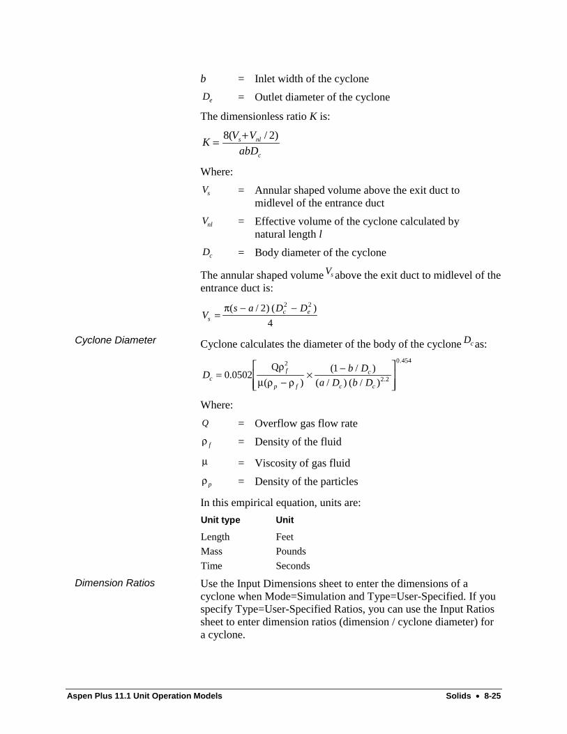
Aspen Plus 11.1 Unit Operation Models Solids • 8-25
b = Inlet width of the cyclone
De = Outlet diameter of the cyclone
The dimensionless ratio K is:
c
nls
abD
VVK
)2/(8 +=
Where:
Vs = Annular shaped volume above the exit duct tomidlevel of the entrance duct
Vnl = Effective volume of the cyclone calculated bynatural length l
Dc = Body diameter of the cyclone
The annular shaped volume Vs above the exit duct to midlevel of theentrance duct is:
Vs a D D
sc e=
− −π( / ) ( )2
4
2 2
Cyclone calculates the diameter of the body of the cyclone Dc as:
Db D
a D b Dcf
p f
c
c c
=−
×−
0.0502Q
(
2ρµ ρ ρ )
( / )
( / ) ( / ) .
.1
2 2
0 454
Where:
Q = Overflow gas flow rate
ρ f = Density of the fluid
µ = Viscosity of gas fluid
ρp = Density of the particles
In this empirical equation, units are:
Unit type Unit
Length Feet
Mass Pounds
Time Seconds
Use the Input Dimensions sheet to enter the dimensions of acyclone when Mode=Simulation and Type=User-Specified. If youspecify Type=User-Specified Ratios, you can use the Input Ratiossheet to enter dimension ratios (dimension / cyclone diameter) fora cyclone.
Cyclone Diameter
Dimension Ratios

8-26 • Solids Aspen Plus 11.1 Unit Operation Models
The dimension ratios and some default values of the two built-inconfigurations are:
Dimension ratio (dimension/cyclone diameter)
Type = Highefficiency
Type = Mediumefficiency
Cyclone diameter 1.0 1.0
Inlet height 0.5 0.75
Inlet width 0.2 0.375
Length of overflow 0.5 0.875
Diameter of overflow 0.5 0.75
Length of cone section 1.5 1.50
Overall length 4.0 4.0
Diameter of underflow 0.375 0.375
Number of gas turn in cyclone 7.0 4.0
Maximum diameter (m) 1.5 5.0
Minimum diameter (m) 0.1 0.1
Cyclone calculates the dimensions of the built-in cyclones usingthese ratios and the cyclone diameter you specify. The built-inconfigurations (Type=High or Medium) may not be the bestdesigns. It is recommended that you enter dimensions or dimensionratios, if available.
Use the Vane Constant field on the Input Specifications sheet tospecify the vane constant. The vane constant varies with theconfiguration of the inlet duct. In the common configuration, theinlet duct terminates at the wall of the cyclone. The vane constantis 16. To reduce friction loss, extend the duct into the interior ofthe cyclone. When the duct is in the middle of the cycloneseparator, the vane constant is 7.5.
Vane Constant
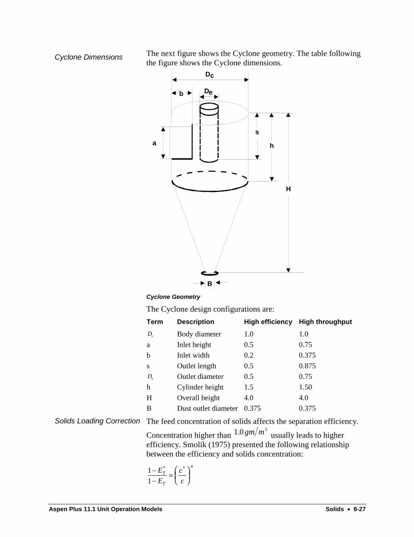
Aspen Plus 11.1 Unit Operation Models Solids • 8-27
The next figure shows the Cyclone geometry. The table followingthe figure shows the Cyclone dimensions.
a
De
Dc
b
s
h
H
B
Cyclone Geometry
The Cyclone design configurations are:
Term Description High efficiency High throughput
Dc Body diameter 1.0 1.0
a Inlet height 0.5 0.75
b Inlet width 0.2 0.375
s Outlet length 0.5 0.875De Outlet diameter 0.5 0.75
h Cylinder height 1.5 1.50
H Overall height 4.0 4.0
B Dust outlet diameter 0.375 0.375
The feed concentration of solids affects the separation efficiency.
Concentration higher than 1 0 3. gm m usually leads to higherefficiency. Smolik (1975) presented the following relationshipbetween the efficiency and solids concentration:
1
1
−−
=
E
E
c
cT
T
a* *
Cyclone Dimensions
Solids Loading Correction
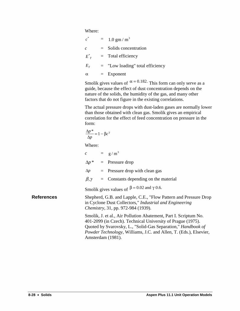
8-28 • Solids Aspen Plus 11.1 Unit Operation Models
Where:
c* = 1.0 gm / m3
c = Solids concentration
E T* = Total efficiency
ET = "Low loading" total efficiency
α = Exponent
Smolik gives values of α = 0.182. This form can only serve as aguide, because the effect of dust concentration depends on thenature of the solids, the humidity of the gas, and many otherfactors that do not figure in the existing correlations.
The actual pressure drops with dust-laden gases are normally lowerthan those obtained with clean gas. Smolik gives an empiricalcorrelation for the effect of feed concentration on pressure in theform:
∆∆p
pc
* = −1 β γ
Where:
c = g / m3
∆p * = Pressure drop
∆p = Pressure drop with clean gas
β γ, = Constants depending on the material
Smolik gives values of β γ= 0.02 and 0.6.
Shepherd, G.B. and Lapple, C.E., "Flow Pattern and Pressure Dropin Cyclone Dust Collectors," Industrial and EngineeringChemistry, 31, pp. 972-984 (1939).
Smolik, J. et al., Air Pollution Abatement, Part I. Scriptum No.401-2099 (in Czech). Technical University of Prague (1975).Quoted by Svarovsky, L., "Solid-Gas Separation," Handbook ofPowder Technology, Williams, J.C. and Allen, T. (Eds.), Elsevier,Amsterdam (1981).
References
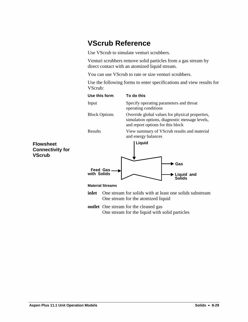
Aspen Plus 11.1 Unit Operation Models Solids • 8-29
VScrub ReferenceUse VScrub to simulate venturi scrubbers.
Venturi scrubbers remove solid particles from a gas stream bydirect contact with an atomized liquid stream.
You can use VScrub to rate or size venturi scrubbers.
Use the following forms to enter specifications and view results forVScrub:
Use this form To do this
Input Specify operating parameters and throatoperating conditions
Block Options Override global values for physical properties,simulation options, diagnostic message levels,and report options for this block
Results View summary of VScrub results and materialand energy balances
Gas
Liquid
Feed Gaswith Solids Liquid and
Solids
Material Streams
inlet One stream for solids with at least one solids substreamOne stream for the atomized liquid
outlet One stream for the cleaned gasOne stream for the liquid with solid particles
FlowsheetConnectivity forVScrub

8-30 • Solids Aspen Plus 11.1 Unit Operation Models
Use the VScrub Input Specifications sheet to specify operatingconditions and parameters for sizing or rating calculations.
To perform thesecalculations
Set Mode = Enter scrubber VScrub calculates
Rating Simulation Throat DiameterThroat Length
Separation efficiencyPressure drop
Sizing † Design Separationefficiency
Liquid flow rateThroat diameterThroat lengthPressure drop
† Because the required liquid flow rate is varied to meet theefficiency, the material balance is not satisfied if the calculatedliquid flow rate is different from the rate you enter.
In both modes, VScrub also calculates the particle sizedistributions of the solids in the outlet streams.
VScrub assumes that the liquid stream is introduced before or atthe beginning of the scrubber throat. It also assumes the separationof the solid particles from the gas stream occurs only at thescrubber throat.
VScrub calculates the pressure drop (Yung, S. et al., 1977) ∆ pacross the throat of the scrubber as:
( )∆pV
g
Q
Qx x xl t
c
l
g
=
− + −
21
22 4 2ρ
Where:
ρl = Density of the liquid
Vt = Relative velocity of gas to liquid at the throat
gc = Conversion factor in Newton's law of motion
Q
Ql
g
= Liquid to gas volume flow rate
x = Dimensionless throat length defined by:
xl C
Dt D g
d l
= +3
161
ρρ
Where:
lt = Throat length
CD = Drag coefficient, as a function of the Reynolds
number (Dickinson and Marshall, 1968) N Re .
CN
ND = + +. ( . ).2224
1 015 0 6
ReRe
Specifying VScrub
Pressure Drop

Aspen Plus 11.1 Unit Operation Models Solids • 8-31
ρg = Density of the gas
ρl = Density of the liquid
Dd = Drop diameter (Sauter mean), defined by(Nukiyama, S., Tanasawa, Y. 1939):
585597
10000 5 0 45 1 5
V
Q
Qt
l
l
l
l l
l
g
σρ
µσ ρ
+
. . .
Where:
σ l = Surface tension
µ l = Viscosity of liquid
The separation efficiency (Yung, S., et al., 1978) ηo is defined as:
ηo
Mass flow rate of particles in outlet liquid stream
Mass flow rate of particles in inlet gas stream=
= ∑ S
Total inlet flow rate of solidsi iη
Where:
ηi = Efficiency for size increment i
Si = Mass flow rate of size increment i
Yung, S. et al., Journal of the Air Pollution Control Association,27, 348 (1977).
Dickinson, D.R. and Marshall, W.R., AIChE Journal, 14, 541,(1968).
Nukiyama, S. and Tanasawa, Y., Transcripts of the Society ofMechanical Engineers (Japan), 5, 63 (1939).
Yung, S. et al., Environmental Science and Technology, 12, 456(1978).
Separation Efficiency
References

8-32 • Solids Aspen Plus 11.1 Unit Operation Models
ESP ReferenceUse ESP to simulate dry electrostatic precipitators.
Dry electrostatic precipitators separate solids from a gaseousstream. Electrostatic precipitators have vertically mountedcollecting plates with discharge wires. The wires are parallel andpositioned midway between the plates.
The corona discharge of the high-voltage wire electrodes firstcharges the solid particles in the inlet gas stream. Then theelectrostatic field of the collecting plate electrodes removes thesolids from the gas stream.
You can use ESP to size or rate electrostatic precipitators.
Use the following forms to enter specifications and view results forESP:
Use this form To do this
Input Specify operating parameters and dielectricconstants and precipitator dimensions
BlockOptions Override global values for physical properties,simulation options, diagnostic message levels,and report options for this block
Results View summary of ESP results and material andenergy balances
Feed
Gas
Solids
Material Streams
inlet One material stream with at least one solids substream
outlet One material stream for the cleaned gasOne material stream for the solids
Each solids substream must have a particle size distribution (PSD)attribute.
FlowsheetConnectivity for ESP

Aspen Plus 11.1 Unit Operation Models Solids • 8-33
Use the Input Specifications sheet to specify parameters for sizingor rating calculations.
To performthesecalculations
Set Mode= Enter ESP calculates
Rating Simulation Number of platesPlate heightPlate length
Separation efficiencyPower requiredCorona voltagePressure dropPrecipitator width
Sizing Design Separationefficiency
Number of platesPrecipitator dimensionsPower requiredPressure drop
You can specify maximum dimensions for sizing calculations onthe Input Specifications sheet.
The velocity of gas should be between 1 and 2.5 m/sec (for platespacing 200 and 300 mm). If the gas velocity is larger than 3 m/sor less than 0.5 m/s, then the models for efficiency and pressuredrop are not valid. This is because the transport of fine particles byturbulent diffusion may become more significant than transport byelectrostatic force.
ESP models wire-and-plate precipitators with relatively high dust
concentration ( ).≥ 1011 particles / m or 0.1 kg / m3 3
If the particleconcentration is too low, ESP may overestimate the results. ESP isnot suitable for a cylindrical electrostatic precipitator.
The separation efficiency is defined as (Crawford, M. 1976):
ηov
Mass outlet flow rate of solids
Total mass flow rate of the inlet solids substream=
ηπµov
nvs
nvo
s ps cC
C
X L q E C
dWV= −
−
1
3exp
( )
Where:
Cnvs = Particle concentration at Xs
Cnvo = Particle concentration at inlet
Xs = Point at which all particles have acquired asaturation charge
L = Plate length
qps = Particle saturation charge
Ec = Collecting field strength ( . ( ))= 0 25 Eo
Specifying ESP
Operating Ranges
Separation Efficiency

8-34 • Solids Aspen Plus 11.1 Unit Operation Models
C = Conningham correction factor
µ = Viscosity of the gas
d = Particle diameter
W = Distance between wires and plates
V = Actual gas velocity through the precipitator
The point at which all particles have acquired a saturation chargeXs , is defined as:
XdW s V C C
E C E Ws E rsw nvo nvs
o c c w
=−
−µε
2
0 00 332 0 8
( )
. ( . )
Where:
sw = Distance between two wires
εo = Electric permissivity constant =−8 85 10 12. x c / vm
Eo = Corona field strength (White, H. J., 1963)
ro = Corona radius
The collecting field strength Ec , is defined as:
E V fT P
TP
T P
TP rc Bo
o
o
o o
= +
−0 25 0 03. .
Where:
VB = Breakdown voltage
f = Roughness factor of wire
To = Atmospheric temperature
Po = Atmospheric pressure
T = Temperature
P = Pressure
The particle concentration at the point where the particles first
have saturation charge, Cnvs is:
Ck
kd
E Ws E r
Ws E E r Ws rnvs
c w o o
w c o o w o
=+ −
+ −0 212 2 08
0 427 2 05332
. ( ) .
. ( . )
Where:
k = Dielectric constant ( / )= ε εo

Aspen Plus 11.1 Unit Operation Models Solids • 8-35
The particle saturation charge, qps is:
qk d
kE
E r
Ws
r
Wspso
co o
w
o
w
=+
+ −
3
2
2
3
2 5 2
3
1 252πε . .
ESP calculates the pressure drop across the precipitator as:
∆p Vg g= 45 5 2. ρ
Where:
ρg = Gas density
Vg = Gas velocity
The power required (White, H. J., 1963) Pw to meet a specifiedseparation efficiency is:
P Qw ov= −52 75 1. ln( )η
Where:
Q = Volumetric gas flow rate
The models used in ESP are valid for inlet gas velocities rangingfrom 0.5 to 3 m/s. Outside this range, transport by turbulentdiffusion becomes more significant than by electrostatic force andlarge errors should be expected.
You can use ESP to model the separation of fine particles withdiameters ranging from 0.01 to 10 microns. ESP is accurate whenthe inlet particle concentration is high( ).≥ 1011 particles / m or 0.1 kg / m3 3
If the concentration is toolow, the model tends to overestimate the separation efficiency.
Crawford, M., Air Pollution Control Theory, Chapter 8:Electrostatic Precipitation, p. 298-358. McGraw-Hill, New York,1976.
White, H.J., Industrial Electrostatic Precipitation, 204, pp. 91-92(1963).
Pressure Drop
Required Power
Gas Velocity
Particle Diameter
References
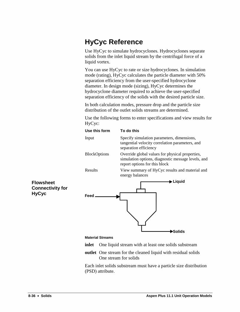
8-36 • Solids Aspen Plus 11.1 Unit Operation Models
HyCyc ReferenceUse HyCyc to simulate hydrocyclones. Hydrocyclones separatesolids from the inlet liquid stream by the centrifugal force of aliquid vortex.
You can use HyCyc to rate or size hydrocyclones. In simulationmode (rating), HyCyc calculates the particle diameter with 50%separation efficiency from the user-specified hydrocyclonediameter. In design mode (sizing), HyCyc determines thehydrocyclone diameter required to achieve the user-specifiedseparation efficiency of the solids with the desired particle size.
In both calculation modes, pressure drop and the particle sizedistribution of the outlet solids streams are determined.
Use the following forms to enter specifications and view results forHyCyc:
Use this form To do this
Input Specify simulation parameters, dimensions,tangential velocity correlation parameters, andseparation efficiency
BlockOptions Override global values for physical properties,simulation options, diagnostic message levels, andreport options for this block
Results View summary of HyCyc results and material andenergy balances
Feed
Liquid
SolidsMaterial Streams
inlet One liquid stream with at least one solids substream
outlet One stream for the cleaned liquid with residual solidsOne stream for solids
Each inlet solids substream must have a particle size distribution(PSD) attribute.
FlowsheetConnectivity forHyCyc

Aspen Plus 11.1 Unit Operation Models Solids • 8-37
Use the Input Specifications sheet to specify hydrocycloneoperating conditions.
To performthesecalculations
Enter HyCyc calculates
Rating SimulationModeHydrocyclonediameter
Separation efficiencyParticle diameter with 50% separationefficiencyPressure drop, particle size distributionof outlet solids stream
Sizing Design ModeSeparationefficiency
Hydrocyclone diameterPressure drop, particle size distributionof outlet solids stream
To obtain practical dimensions when sizing hydrocyclones, enterthe:
• Maximum diameter of the hydrocyclone
• Maximum pressure drop allowed across the hydrocyclone
HyCyc designs multiple hydrocyclones in parallel if one of thefollowing conditions exists:
• The calculated diameter is greater than the maximum specifieddiameter.
• The calculated pressure drop is greater than the maximumspecified pressure drop.
HyCyc uses empirical and semi-empirical correlations. Expectunreliable results when operating conditions (Bradley, D., 1965)are outside the ranges of experimental data on which the modelsare based. In general, your data should fall within these ranges:
• Particle diameter between and (5 to 200 micrometers)
• Hydrocyclone diameter between 0.01 and 0.6 m
• Pressure drop between 35 and 345 kPa
• Separation efficiency between 2% and 98%
The solids concentration should be less than 11% of the volumefraction, or less than 25% of the weight fraction.
Separation efficiency E is defined as:
Emass underflow rate of solids
mass feedflow rate of solids=
Reduced efficiency E’ is defined as the fraction of feed solids thatgo to the underflow minus the fraction of the feed liquid that alsogoes to the underflow.
Specifying HyCyc
Operating Ranges
Separation Efficiency

8-38 • Solids Aspen Plus 11.1 Unit Operation Models
′ =−−
EE R
Rf
f1
Where Rf is the volumetric ratio of underflow to feed flow (see
Material Split).
The reduced efficiency is obtained from the following equation:
′ = − − −
E
d
d100 1 0 115
50
3
exp .
Where:
d = Diameter of the solid particles to be separated
50d = Particle diameter for which 50% of feed passesthrough underflow
In turn, 50d is obtained from the following equation which includesoperational and geometric parameters (Bradley, D., 1965):
d D
D
D R
Qc
i
nc f50
2
0 53 0 38 1
2=
−−
( . ) ( )
( )tan
.
αµ
σ ρθ
Where:
Q = Volumetric flow rate at inlet
Dc = Chamber diameter
Di = Inlet diameter
n = Power of R in the tangential velocity distributionfunction
α = Inlet velocity loss coefficient
σ = Density of solid
Rf = Underflow rate/feed rate
θ = Cone angle
ρ = Density of liquid
µ = Viscosity of liquid
HyCyc splits the feed according to the following empiricalcorrelation (Moder, J.M. and Dahlstrom, D.A., 1952):
44.4.4)( −= QD
DS
o
uβ
Where:
Material Split

Aspen Plus 11.1 Unit Operation Models Solids • 8-39
S = Volume split = underflow rate/overflow rate
β = A constant, 6.13
Du = Diameter for underflow
Do = Diameter for overflow
Q = Inlet volumetric flow rate (gal/min)
The flow ratio Rf (underflow rate/feed rate) is then obtained by:
11
1− =
+R
Sf
The following empirical correlation gives the tangential velocity V(Dahlstrom, D.A., 1954) in a hydrocyclone at a radius R:
n
ci
n DVconstantVR
==
2α
Where:
α = Inlet velocity loss coefficient
Vi = Inlet velocity
Dc = Diameter of the hydrocyclone
n = Exponent of radial dependence
R = Radius
For most cases, α and n are determined experimentally to be 0.45
and 0.8. These two variables are then used to determine 50d .
Common hydrocyclones have the following ranges of dimensionratios (dimension/chamber diameter):Inlet diameter: 1/7 to 1/3
Length: 4 to 12
Overflowdiameter:
1/8 to 1/2.3
Underflowdiameter:
1/10 to 1/5
Cone angle: 9 deg. to 20 deg.
For the pressure drop correlation to be valid (overflowdiameter/underflow diameter) should be 0.6 to 2.0. HyCyc uses theempirical pressure drop correlation (Dahlstrom, D.A., 1954):
Q
HD Do i0 5
0 96 38... ( )= ×
Where:
Tangential Velocity
Dimension Ratios
Pressure Drop

8-40 • Solids Aspen Plus 11.1 Unit Operation Models
Q = Volumetric flow rate (US gallons/minute) at the inlet
H = Height of fluid (feet) or length of vortex finder
Do = Overflow diameter
Di = Inlet diameter
The next figure shows the HyCyc geometry.
Inlet Di
L
θ
Do
Dc
Du
Hydrocyclone Dimensions
The following table describes the HyCyc dimensions.
Term Description
Dc Chamber diameter
Di Inlet diameter
Do Overflow diameter
Du Underflow diameter
L Length of hydrocyclone
θ Cone angle
Bradley, D., The Hydrocyclone, 1st edition, Pergamon Press,London (1965).
Yoshioka, H. and Hatta, Y., Kagaku Kagolar, ChemicalEngineering, Japan, 19, 633 (1955).
HydrocycloneDimensions
References

Aspen Plus 11.1 Unit Operation Models Solids • 8-41
Dahlstrom, D.A., "Mineral Engineering Techniques," ChemicalEngineering Progress Symposium Series 50, No. 15, 41 (1954).
Moder, J.M. and Dahlstrom, D.A., Chemical EngineeringProgress, 48,75 (1952).
8-42 • Solids Aspen Plus 11.1 Unit Operation Models
CFuge ReferenceUse CFuge to simulate centrifuge filters. The centrifuge filtersseparate liquids and solids by the centrifugal force of a rotatingbasket.
Use CFuge to rate or size centrifuge filters.
CFuge assumes that the separation efficiency of the solids equals1, so that the outlet filtrate stream contains no residual solids.
Use the following forms to enter specifications and view results forCFuge:
Use this form To do this
Input Specify centrifuge and filter cake parameters andcentrifuge dimensions
BlockOptions Override global values for physical properties,simulation options, diagnostic message levels,and report options for this block
Results View summary of CFuge results and materialand energy balances
Feed
Liquid
Solids
Material Streams
inlet One material stream with at least one solids substream
outlet One material stream for the liquidOne material stream for the solids
If you specify the particle size distribution (PSD), CFugecalculates the average particle size.
FlowsheetConnectivity forCFuge

Aspen Plus 11.1 Unit Operation Models Solids • 8-43
Use the Input Specifications sheet to specify operating conditionsand the Input FilterCake sheet to specify filter cake properties.
To performthesecalculations
Enter CFuge calculates
Rating DiameterRate of revolutionFilter cake properties
Filtrate flow rateFilter cake moisture contentHeight of centrifuge basket
Sizing List of centrifuge diametersand rates of revolutionFilter cake moisture content(CFuge estimates if notentered)
Filtrate flow rateFilter cake moisture contentHeight of centrifuge basket
For sizing calculations, CFuge also calculates the liquid-handlingcapacities of all of the centrifuges you specify. CFuge selects thecentrifuge with a liquid-handling capacity greater than or equal tothe required filtrate flow rate. If more than one centrifuge satisfiesthis criterion, CFuge selects the one with the smallest capacity. Ifnone of the centrifuges satisfies this criterion, CFuge selects theone with the highest filtrate flow rate.
In both rating and sizing calculations, CFuge calculates the contentand height of the centrifuge basket.
Use the Input FilterCake sheet to specify:
• Cake resistance
• Moisture Content
• Sphericity
• Medium resistance
• Porosity
• The average diameter of the solid particles in the cake
The filter cake moisture content is the ratio of the mass flow rate ofliquid to that of the solid in the outlet solids stream. The filter cakemoisture content is an important design parameter. You shouldprovide it if possible. If you do not enter it, CFuge calculates anestimate from the average particle diameter and cake parameters(Dombrowski, H.S., and Brownell, L.E., 1954).
If you enter the particle size distribution (PSD) of the inlet solidstream, CFuge calculates the average particle diameter, so you donot need to enter average diameter on the Input FilterCake sheet.
Specifying CFuge
Filter CakeCharacteristics
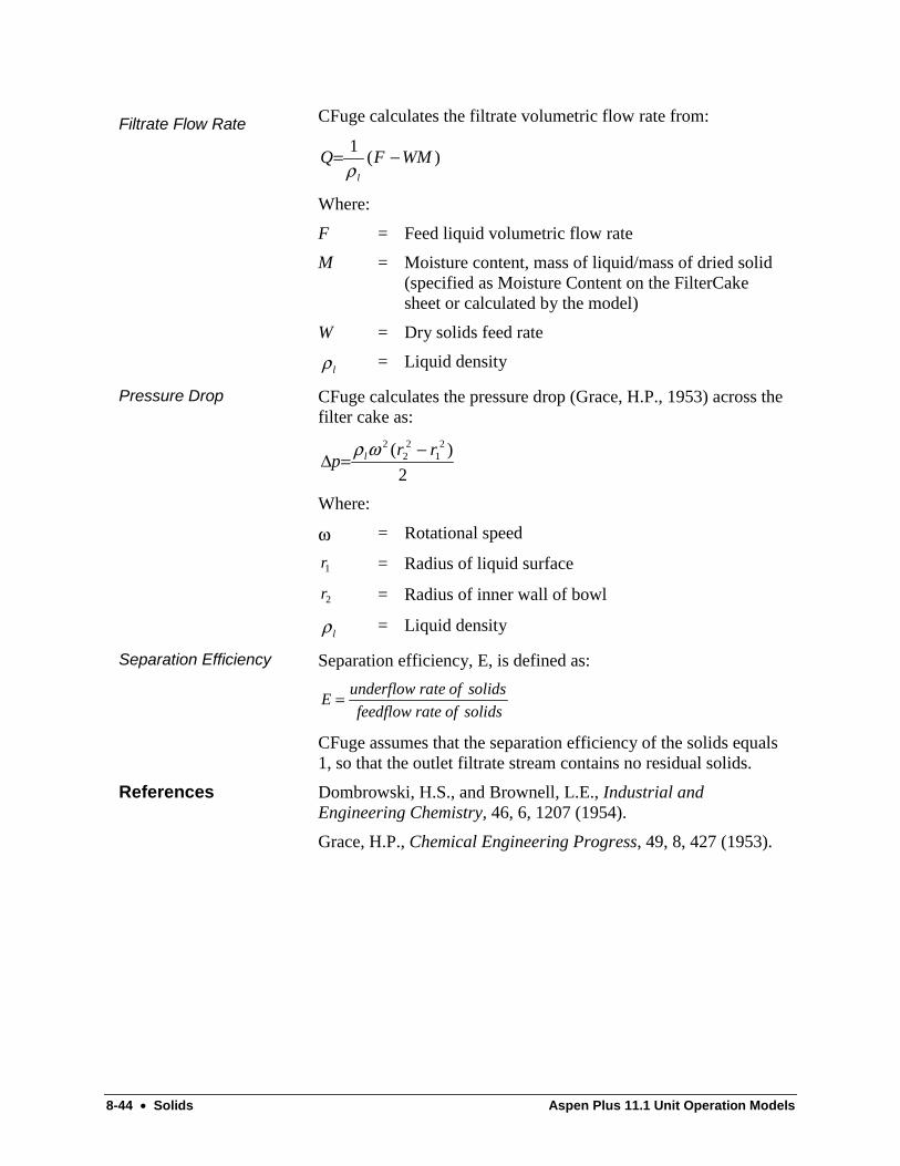
8-44 • Solids Aspen Plus 11.1 Unit Operation Models
CFuge calculates the filtrate volumetric flow rate from:
)(1
WMFQl
−=ρ
Where:
F = Feed liquid volumetric flow rate
M = Moisture content, mass of liquid/mass of dried solid(specified as Moisture Content on the FilterCakesheet or calculated by the model)
W = Dry solids feed rate
lρ = Liquid density
CFuge calculates the pressure drop (Grace, H.P., 1953) across thefilter cake as:
2
)( 21
22
2 rrp l −=∆
ωρ
Where:
ω = Rotational speed
r1 = Radius of liquid surface
r2 = Radius of inner wall of bowl
lρ = Liquid density
Separation efficiency, E, is defined as:
Eunderflow rate of solids
feedflow rate of solids=
CFuge assumes that the separation efficiency of the solids equals1, so that the outlet filtrate stream contains no residual solids.
Dombrowski, H.S., and Brownell, L.E., Industrial andEngineering Chemistry, 46, 6, 1207 (1954).
Grace, H.P., Chemical Engineering Progress, 49, 8, 427 (1953).
Filtrate Flow Rate
Pressure Drop
Separation Efficiency
References

Aspen Plus 11.1 Unit Operation Models Solids • 8-45
Filter ReferenceUse Filter to simulate continuous rotary vacuum filters. You canuse Filter to rate or size rotary vacuum filters.
Filter assumes the separation efficiency of the solids equals 1, sothat the outlet filtrate stream contains no residual solids.
Use the following forms to enter specifications and view results forFilter:
Use this form To do this
Input Specify filter and filter cake parameters
BlockOptions Override global values for physical properties,simulation options, diagnostic message levels,and report options for this block
Results View summary of Filter results and material andenergy balances
Feed
Filtrate
Solids
Material Streams
inlet One material stream with at least one solids substream
outlet One material stream for the liquid filtrateOne material stream for the solids
Use the Input Specifications sheet to specify operating conditionsand parameters.
To perform thesecalculations
Enter Filtercalculates
Rating SimulationDiameterWidthRate of revolutionFilter cake characteristics (optional)
Pressure dropacross filter
Sizing DesignMaximum allowable pressure dropacross the filter cake and mediumRate of revolutionFilter cake characteristics (optional)Width to diameter ratio (optional)
DiameterWidth
FlowsheetConnectivity for Filter
Specifying Filter

8-46 • Solids Aspen Plus 11.1 Unit Operation Models
In both calculation modes, Aspen Plus determines the following:
• Filtrate volumetric flow rate
• Cake thickness
• Mass fraction of solids in the solids filter cake
Filter assumes:
• The cake thickness is greater than 0.00635 m.
• The capillary number is greater than 1.
• The filter cake is incompressible or compacted uniformlythroughout its thickness (Dombrowski, H. S., and Brownell,L.E., 1954).
When the specific cake resistance α at the required pressure drop∆P is not available, Filter can estimate it using the followingempirical correlation:
( )α α= OkP∆
Where:
αO = Specific cake resistance at unit pressure drop
k = Cake compressibility
You can use this equation for interpolation and short-range
extrapolation when some experimental data of αO and ∆P are
available. αO is the intercept of the log-log plot of α versus ∆P. α
and αO both have the units determined by the specified units set,and ∆P is always in Pascals.
Use the Average Diameter field on the FilterCake sheet to specifythe average diameter of solid particles in the filter cake. If youenter the particle size distribution (PSD) of the inlet solid stream,Filter calculates the average particle size.
Filter calculates the pressure drop (Brownell, L.E., and Katz, D.I.,1947) across the filter cake with:
Q RHV RHp V
W= =
ω
ωθµα
21 2
∆/
Where:
Q = Filtrate volume flow rate
ω = Angular velocity
R = Radius
H = Width
Filter CakeCharacteristics
Pressure Drop

Aspen Plus 11.1 Unit Operation Models Solids • 8-47
V = Filtrate volume per unit area
∆p = Pressure drop
θ = Wetting angle
µ = Viscosity
α = Filtration resistance
W = Solid mass per unit area
Separation efficiency, E, is defined as:
Eunderflow rate of solids
feedflow rate of solids=
Filter assumes the separation efficiency of the solids equals 1, sothat the outlet filtrate stream contains no residual solids.
Brownell, L.E. and Katz, D. I., Chemical Engineering Progress,43, 11, 601 (1947).
Dombrowski, H.S. and Brownell, L.E., Industrial and EngineeringChemistry, 46, 6, 1207 (1954).
Separation Efficiency
References
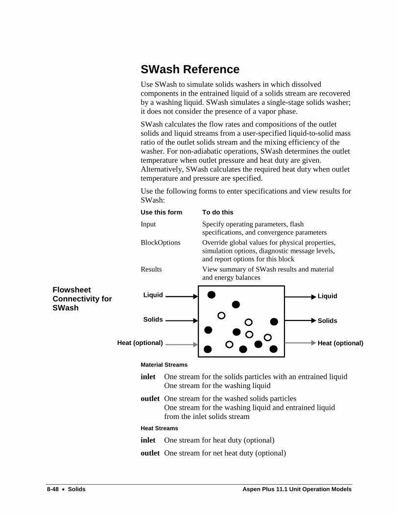
8-48 • Solids Aspen Plus 11.1 Unit Operation Models
SWash ReferenceUse SWash to simulate solids washers in which dissolvedcomponents in the entrained liquid of a solids stream are recoveredby a washing liquid. SWash simulates a single-stage solids washer;it does not consider the presence of a vapor phase.
SWash calculates the flow rates and compositions of the outletsolids and liquid streams from a user-specified liquid-to-solid massratio of the outlet solids stream and the mixing efficiency of thewasher. For non-adiabatic operations, SWash determines the outlettemperature when outlet pressure and heat duty are given.Alternatively, SWash calculates the required heat duty when outlettemperature and pressure are specified.
Use the following forms to enter specifications and view results forSWash:
Use this form To do this
Input Specify operating parameters, flashspecifications, and convergence parameters
BlockOptions Override global values for physical properties,simulation options, diagnostic message levels,and report options for this block
Results View summary of SWash results and materialand energy balances
Liquid
Solids
Liquid
Solids
Heat (optional) Heat (optional)
Material Streams
inlet One stream for the solids particles with an entrained liquidOne stream for the washing liquid
outlet One stream for the washed solids particlesOne stream for the washing liquid and entrained liquidfrom the inlet solids stream
Heat Streams
inlet One stream for heat duty (optional)
outlet One stream for net heat duty (optional)
FlowsheetConnectivity forSWash
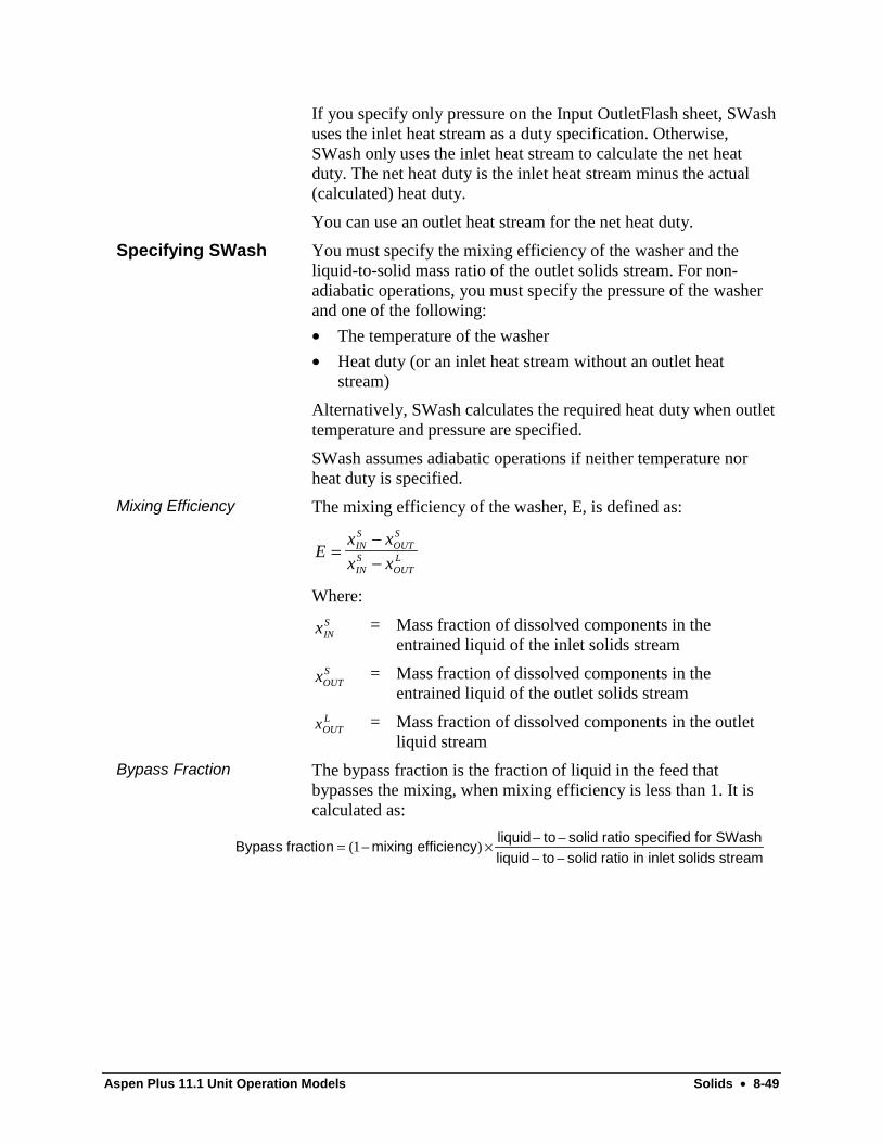
Aspen Plus 11.1 Unit Operation Models Solids • 8-49
If you specify only pressure on the Input OutletFlash sheet, SWashuses the inlet heat stream as a duty specification. Otherwise,SWash only uses the inlet heat stream to calculate the net heatduty. The net heat duty is the inlet heat stream minus the actual(calculated) heat duty.
You can use an outlet heat stream for the net heat duty.
You must specify the mixing efficiency of the washer and theliquid-to-solid mass ratio of the outlet solids stream. For non-adiabatic operations, you must specify the pressure of the washerand one of the following:
• The temperature of the washer
• Heat duty (or an inlet heat stream without an outlet heatstream)
Alternatively, SWash calculates the required heat duty when outlettemperature and pressure are specified.
SWash assumes adiabatic operations if neither temperature norheat duty is specified.
The mixing efficiency of the washer, E, is defined as:
Ex x
x xINS
OUTS
INS
OUTL=
−−
Where:
xINS = Mass fraction of dissolved components in the
entrained liquid of the inlet solids stream
xOUTS = Mass fraction of dissolved components in the
entrained liquid of the outlet solids stream
xOUTL = Mass fraction of dissolved components in the outlet
liquid stream
The bypass fraction is the fraction of liquid in the feed thatbypasses the mixing, when mixing efficiency is less than 1. It iscalculated as:
Bypass fraction mixing efficiencyliquid to solid ratio specified for SWashliquid to solid ratio in inlet solids stream
= − × − −− −
( )1
Specifying SWash
Mixing Efficiency
Bypass Fraction
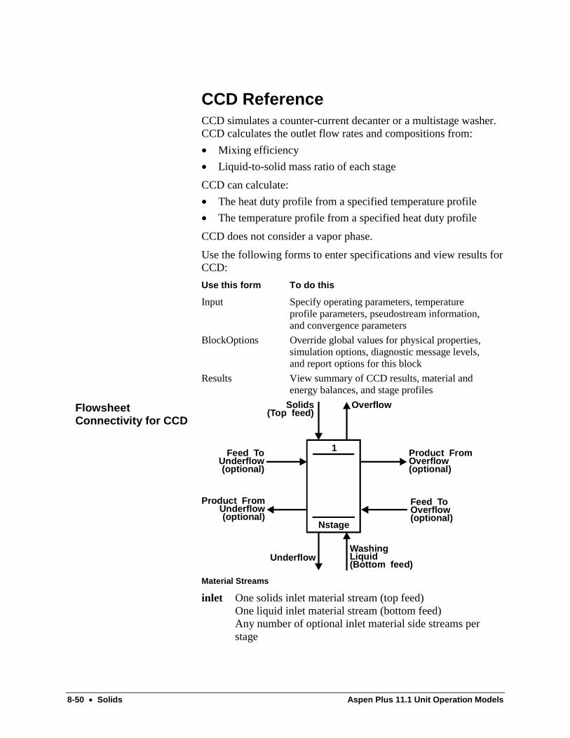
8-50 • Solids Aspen Plus 11.1 Unit Operation Models
CCD ReferenceCCD simulates a counter-current decanter or a multistage washer.CCD calculates the outlet flow rates and compositions from:
• Mixing efficiency
• Liquid-to-solid mass ratio of each stage
CCD can calculate:
• The heat duty profile from a specified temperature profile
• The temperature profile from a specified heat duty profile
CCD does not consider a vapor phase.
Use the following forms to enter specifications and view results forCCD:
Use this form To do this
Input Specify operating parameters, temperatureprofile parameters, pseudostream information,and convergence parameters
BlockOptions Override global values for physical properties,simulation options, diagnostic message levels,and report options for this block
Results View summary of CCD results, material andenergy balances, and stage profiles
OverflowSolids(Top feed)
Product FromOverflow (optional)
Feed ToOverflow(optional)
WashingLiquid(Bottom feed)
Underflow
Product FromUnderflow (optional)
Feed ToUnderflow (optional)
Nstage
1
Material Streams
inlet One solids inlet material stream (top feed)One liquid inlet material stream (bottom feed)Any number of optional inlet material side streams perstage
FlowsheetConnectivity for CCD
Aspen Plus 11.1 Unit Operation Models Solids • 8-51
outlet One top product stream (overflow)One bottom product stream (underflow)One optional stream per stage for the solids (underflow)One optional stream per stage for the liquid (overflow)Any number of pseudoproduct streams (optional)
Any number of pseudoproduct streams can represent internalunderflows or overflows. A pseudoproduct stream does not affectthe results of the simulation.
Use the CCD Input Specifications sheet to enter the number ofstages, pressure, mixing efficiency, and liquid-to-solid mass ratio.
Use the CCD Input Streams to enter feed, product, and optionalheat stream locations.
On the CCD Input Temp-DutyProfiles sheet, note the following:
If you enter CCD calculates
Stage temperature Stage heat duty.
Stage heat duty Stage temperature.
Stage overall heat transfer coefficient Stage temperature.
You cannot enter both temperature profiles and heat duties oroverall heat transfer coefficients. If you enter stage heat dutyand/or an overall heat transfer coefficient, and you do not entervalues for all stages, the system assumes unspecified values to bezero. Enter the medium temperature of each stage when you enteroverall heat transfer coefficients. Use the Estimated Temperaturefield to enter estimated stage temperatures.
Note: CCD interpolates unspecified values and, by default,assumes them to be the same as the ambient temperature.
Use the CCD Input PseudoStream sheet to transfer the internaloverflow or underflow of a stage to a pseudostream.
CCD does not consider the mixing of component attributes andPSDs. CCD assumes all outlet solids streams have the sameattributes and PSD as the solids feed stream to stage one. CCD alsoassumes all outlet liquid streams have the same attributes and PSDas the liquid feed stream throughout the final stages.
For any CCD profile, such as mixing efficiency, liquid-to-solid-ratio, temperature, duty, enter a value for every stage, asinformation becomes available. If you enter only some of thevalues for some stages, CCD generates the complete profile bylinear interpolation of the given values. If you enter only onevalue, CCD assumes a constant profile of that value throughout thewasher.
Specifying CCD
Component Attributes
Multistage WasherProfiles
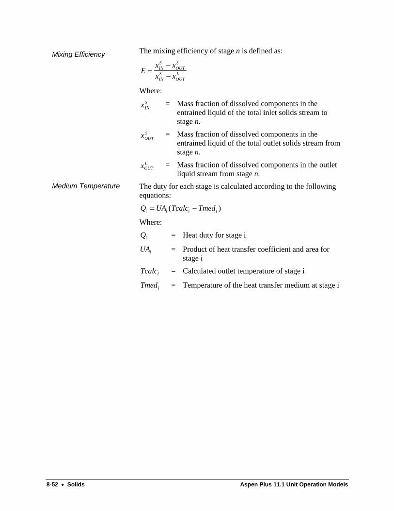
8-52 • Solids Aspen Plus 11.1 Unit Operation Models
The mixing efficiency of stage n is defined as:
Ex x
x xINS
OUTS
INS
OUTL=
−−
Where:
xINS = Mass fraction of dissolved components in the
entrained liquid of the total inlet solids stream tostage n.
xOUTS = Mass fraction of dissolved components in the
entrained liquid of the total outlet solids stream fromstage n.
xOUTL = Mass fraction of dissolved components in the outlet
liquid stream from stage n.
The duty for each stage is calculated according to the followingequations:
Q UA Tcalc Tmedi i i i= −( )
Where:
Qi = Heat duty for stage i
UAi = Product of heat transfer coefficient and area forstage i
Tcalci = Calculated outlet temperature of stage i
Tmedi = Temperature of the heat transfer medium at stage i
Mixing Efficiency
Medium Temperature

Aspen Plus 11.1 Unit Operation Models User Models • 9-1
C H A P T E R 9
User Models
This chapter describes the models that allow you to add customextensions to Aspen Plus.
User and User2 allow you to write your own unit operation modelsas Fortran subroutines. These subroutines must follow theguidelines described in the Aspen Plus User Models referencemanual. User2 can also be used with a unit operation model writtenas an Excel spreadsheet. User3 allows you to use custom orexternal models with equation-oriented formulations. The modelsare:
Model Description Purpose Use For
User User-defined unitoperation model
Model a unit operation using auser-supplied Fortran subroutine
Unit operations with four (or fewer)inlet and outlet streams
User2 User-defined unitoperation model
Model a unit operation using auser-supplied Fortran subroutine.
Unit operations with no limit onnumber of streams
User3 User-defined orexternal unit-operationmodel
Run built-in models from RT-Opt, Aspen EO models from thePML model library, or modelswritten by a user that may containproprietary models
Unit operations with equation-oriented formulations
ACMUser3Aspen CustomModeler models
Models a unit operation usingAspen Custom Modeler
Unit operation models created withAspen Custom Modeler
Hierarchy blocks allow you to organize complex flowsheets in ahierarchical manner. When a user model template containingmultiple blocks is placed on a flowsheet, it automatically appearsinside a Hierarchy block. See the Aspen Plus User Guide, chapter16, for more information on creating these templates. You mayalso use Hierarchy blocks directly, without using a template.
Model Description Purpose Use For
Hierarchy Hierarchical structure Create a hierarchical structure toorganize complex flowsheets.
Container for other blocks

9-2 • User Models Aspen Plus 11.1 Unit Operation Models
User ReferenceUser can model any unit operation model. You must write aFortran subroutine to calculate the values of the outlet streamsbased on the inlet streams and parameters you specify.
User and User2 differ only in the number of inlet and outletstreams allowed and the argument lists to the model subroutine.User is limited to a maximum of four material and one heat orwork inlet stream and a maximum of four material and one heat orwork outlet stream. User2 has no limits on the number of inlet andoutlet streams.
Use the following forms to enter specifications and view results forUser:
Use this form To do this
Input Specify name and parameters for user subroutine,calculation options, and outlet stream conditionsand flash convergence parameters
BlockOptions Override global values for physical properties,simulation options, diagnostic message levels,and report options for this block
Results View summary of User results and material andenergy balances
Heat (optional)Work (optional)
Heat (optional)
Material
Work (optional)
Material Streams
inlet One to four inlet material streams
outlet One to four outlet material streams
Heat Streams
inlet One heat stream (optional)
outlet One heat stream (optional)
Work Streams
inlet One work stream (optional)
outlet One work stream (optional)
FlowsheetConnectivity for User
Aspen Plus 11.1 Unit Operation Models User Models • 9-3
You must specify the name of the subroutine model on the InputSpecifications sheet. You have the option of specifying:
• A report subroutine name
• Size of the integer and real arrays (INT and REAL) passed tothe user model subroutine
• Values of the integer and real arrays passed to the user modelsubroutine
• Length of integer and real workspace vectors
• Thermodynamic conditions of each outlet stream
• Type of flash calculations (vapor, liquid, two-phase, three-phase)
For information on writing Fortran subroutines for user models,see Aspen Plus User Models reference manual.
Specifying User

9-4 • User Models Aspen Plus 11.1 Unit Operation Models
User2 ReferenceUser2 can model any unit operation model. You must write aFortran subroutine to calculate the values of the outlet streamsbased on the inlet streams and parameters you specify.
User and User2 differ only in the number of inlet and outletstreams allowed and the argument lists to the model subroutine.User2 has no limits on the number of inlet and outlet streams. Useris limited to a maximum of four material and one heat or workinlet stream, and a maximum of four material and one heat or workoutlet stream.
Use the following forms to enter specifications and view results forUser2:
Use this form To do this
Setup Specify name and parameters for the usersubroutine, excel file name, values ofconfigured variables, calculation options,outlet stream conditions, and flashconvergence parameters
BlockOptions Override global values for physicalproperties, simulation options, diagnosticmessage levels, and report options for thisblock
Results View summary of User2 results, materialand energy balances, and the values of theconfigured variables.
Heat (optional)Work (optional)
Heat (optional)
Material
Work (optional)
Material Streams
inlet At least one inlet material stream
outlet At least one outlet material stream
Heat Streams
inlet Any number of heat streams (optional)
outlet Any number of heat streams (optional)
Work Streams
inlet Any number of work streams (optional)
outlet Any number of work streams (optional)
FlowsheetConnectivity forUser2

Aspen Plus 11.1 Unit Operation Models User Models • 9-5
You must specify the name of the subroutine model on the User2Input Specifications sheet. You have the option of specifying:
• A report subroutine name
• Size of the integer and real arrays (INT and REAL) passed tothe user model subroutine
• Values of the integer and real arrays passed to the user modelsubroutine
• Length of integer and real workspace vectors
• Thermodynamic conditions of each outlet stream
• Type of flash calculations (vapor, liquid, two-phase, three-phase)
For information on writing Fortran subroutines for user models,see Aspen Plus User Models reference manual.
Specifying User2

9-6 • User Models Aspen Plus 11.1 Unit Operation Models
User3 ReferenceUser3 models are used to simulate features that are not in thestandard Aspen Plus models. They can be one of three types: oldbuilt-in models from RT-Opt (like R3HTUA), Aspen EO modelsfrom the PML model library (like EOTRAYDP) or models writtenby a user that may contain proprietary models (like a reactor).
Use the following forms to enter specifications and view results forthe User3 model:
Use this form To do this
Setup Specify name and parameters for the usersubroutine or Aspen EO model, values ofconfigured variables, calculation options, outletstream conditions, and flash convergenceparameters.
Parameters Specify Jacobian calculation options and runoptions for the Aspen EO model.
Attributes Specify attributes of variables and equations of themodel.
Block Options Override global values for physical properties,simulation options, diagnostic message levels, andreport options for this block.
Results View summary of User3 results, material andenergy balances, and the values of the configuredvariables.
EO Variables Specify equation-oriented variable attributechanges for this block, for the current run only.
EO Input Specify the equation-oriented variables for thisblock.
Spec Groups Specify the specification groups for this block.
Ports Specify the EO variables collected to form portsfor this block.
Heat (optional)Work (optional)
Heat (optional)Material (optional)
Work (optional)
Material (optional)
inlet Any number of inlet material, heat, and/or work streams
outlet Any number of outlet material, heat, and/or work streams
The number and types of streams connected to a User3 modeldepends on the type and configuration of that specific model.
FlowsheetConnectivity forUser3

Aspen Plus 11.1 Unit Operation Models User Models • 9-7
You must specify the name of the model subroutine or Aspen EOmodel on the User3 Input Specifications sheet. You have theoption of specifying:
• A report subroutine name
• Size of the integer and real arrays (INT and REAL) passed tothe user model subroutine
• Values of the integer and real arrays passed to the user modelsubroutine
• Length of integer and real workspace vectors
• Thermodynamic conditions of each outlet stream
• Type of flash calculations (vapor, liquid, two-phase, three-phase)
• Name and location of the configuration file, if using an AspenEO model
• Values of variables on the Attributes form, as needed to makethe problem square
To import a User3 model written for RT-Opt version 3 or 10 withAspen Plus 11:
1 Export an .inp file from the prior version of RT_OPT.
2 Replace the word STRVAR with ANALYZER.
3 Delete any EBS setup scripts.
4 Use the version 11 engine to generate a .bkp file from the .inpfile with the commandASPEN filename /mmbackup /itonly
You can retain your graphics by copying the graphic sectionfrom the previous version’s .bkp file to this newly created .bkpfile.
5 Load the new .bkp file. The User3 forms should be populated.
6 On the top-level EO Configuration EO Options form, selectthe Model Types sheet.
7 From the list of models select USER3. Click AdditionalOptions.
8 In the EO Formulation field, choose mole flows.
The features listed below are not supported in equation-orientedformulation. However, the capabilities are still available for the EOsolution strategy via the Perturbation Layer.
• Flash specifications
• Features which are globally unsupported
Specifying User3
EO Usage Notes forUser3
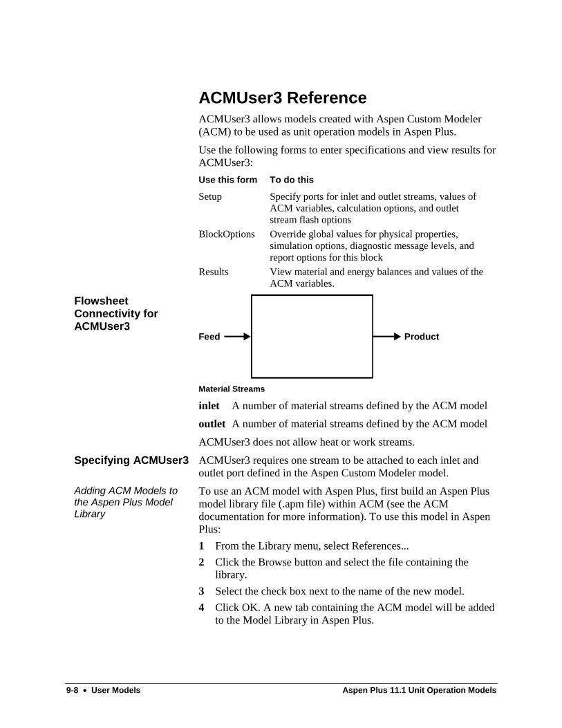
9-8 • User Models Aspen Plus 11.1 Unit Operation Models
ACMUser3 ReferenceACMUser3 allows models created with Aspen Custom Modeler(ACM) to be used as unit operation models in Aspen Plus.
Use the following forms to enter specifications and view results forACMUser3:
Use this form To do this
Setup Specify ports for inlet and outlet streams, values ofACM variables, calculation options, and outletstream flash options
BlockOptions Override global values for physical properties,simulation options, diagnostic message levels, andreport options for this block
Results View material and energy balances and values of theACM variables.
Feed Product
Material Streams
inlet A number of material streams defined by the ACM model
outlet A number of material streams defined by the ACM model
ACMUser3 does not allow heat or work streams.
ACMUser3 requires one stream to be attached to each inlet andoutlet port defined in the Aspen Custom Modeler model.
To use an ACM model with Aspen Plus, first build an Aspen Plusmodel library file (.apm file) within ACM (see the ACMdocumentation for more information). To use this model in AspenPlus:
1 From the Library menu, select References...
2 Click the Browse button and select the file containing thelibrary.
3 Select the check box next to the name of the new model.
4 Click OK. A new tab containing the ACM model will be addedto the Model Library in Aspen Plus.
FlowsheetConnectivity forACMUser3
Specifying ACMUser3
Adding ACM Models tothe Aspen Plus ModelLibrary

Aspen Plus 11.1 Unit Operation Models User Models • 9-9
To save this setting, so that this model will always appear in theModel Library in Aspen Plus, from the Library menu, select SaveDefault.
Now, you may use this model in Aspen Plus in the same way asany other model.

9-10 • User Models Aspen Plus 11.1 Unit Operation Models
Hierarchy ReferenceUse Hierarchy blocks to provide hierarchical structure to complexsimulations. Also, Hierarchy blocks may be added automaticallywhen importing templates into a simulation. Hierarchy blocks maycontain streams and other blocks (even other Hierarchy blocks) aswell other features like design specifications and sensitivityproblems.
Hierarchy blocks contain Setup and Properties forms with some ofthe same information as the top-level Setup and Properties forms.The settings on these forms override the settings on thecorresponding forms at higher-level Hierarchy blocks or the toplevel of the simulation for blocks within the Hierarchy block.
Hierarchy blocks also contain forms for Streams, Blocks,Convergence, Flowsheeting Options, Model Analysis Tools, andResults Summary. These forms are used for working with suchobjects within the Hierarchy block, and they will not affect higher-level Hierarchy blocks or the top level of the simulation exceptthrough the outlet streams of the Hierarchy block.
Use the following forms to enter specifications and view results forHierarchy:
Use this form To do this
Input Specify components for use within the Hierarchyblock, and view connections to streams outsidethe Hierarchy block.
Setup Override settings from the top-level Setup forms.
Properties Override settings from the top-level Propertiesforms.
Streams View or enter information about streams withinthe Hierarchy block.
Blocks View or enter information about blocks withinthe Hierarchy block.
Convergence Define convergence and sequence informationwithin the Hierarchy block.
FlowsheetingOptions
Define design-specs, calculator, transfer, balance,and pressure relief blocks within the Hierarchyblock.
Model AnalysisTools
Define sensitivity, optimization, constraint, anddata-fit blocks within the Hierarchy block.
Results Summary View a summary of stream results within theHierarchy block.

Aspen Plus 11.1 Unit Operation Models User Models • 9-11
A Hierarchy block may have any number of inlet and outletstreams of any types (material, heat, and work). Each externalstream connected to the Hierarchy block is attached to a streamwithin the Hierarchy block. Each stream within the Hierarchyblock with an unconnected source or destination creates a port towhich an external stream may be connected.
Hierarchy normally does not need any specifications.
You may specify the group of components to be shown within theHierarchy block on the Input Specifications Sheet.
To access the flowsheet within a Hierarchy block, double-click onthe block. A new flowsheet window will open, containing theflowsheet inside the Hierarchy block.
FlowsheetConnectivity forHierarchy
Specifying Hierarchy

9-12 • User Models Aspen Plus 11.1 Unit Operation Models
Aspen Plus 11.1 Unit Operation Models Pressure Relief • 10-1
C H A P T E R 10
Pressure Relief
This section contains detailed reference information on theAspen Plus Pres-Relief model for pressure relief calculations. Forinformation on using Pres-Relief, see the Aspen Plus User Guide,Chapter 33.
This section describes the following topics:
• Relief scenarios
• Code compliance checks
• Stream and vessel compositions and conditions
• Rules to size the relief valve piping
• Reactions
• Relief system
• Data tables for pipes and relief devices
• Valve cycling
• Vessel types
• Disengagement models
• Stop criteria
• Solution procedure for dynamic scenarios
• Flow equations
• Calculation and convergence methods
• Vessel insulation credit factor
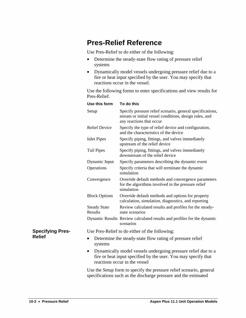
10-2 • Pressure Relief Aspen Plus 11.1 Unit Operation Models
Pres-Relief ReferenceUse Pres-Relief to do either of the following:
• Determine the steady-state flow rating of pressure reliefsystems
• Dynamically model vessels undergoing pressure relief due to afire or heat input specified by the user. You may specify thatreactions occur in the vessel.
Use the following forms to enter specifications and view results forPres-Relief.
Use this form To do this
Setup Specify pressure relief scenario, general specifications,stream or initial vessel conditions, design rules, andany reactions that occur
Relief Device Specify the type of relief device and configuration,and the characteristics of the device
Inlet Pipes Specify piping, fittings, and valves immediatelyupstream of the relief device
Tail Pipes Specify piping, fittings, and valves immediatelydownstream of the relief device
Dynamic Input Specify parameters describing the dynamic event
Operations Specify criteria that will terminate the dynamicsimulation
Convergence Override default methods and convergence parametersfor the algorithms involved in the pressure reliefsimulation
Block Options Override default methods and options for propertycalculation, simulation, diagnostics, and reporting
Steady StateResults
Review calculated results and profiles for the steady-state scenarios
Dynamic Results Review calculated results and profiles for the dynamicscenarios
Use Pres-Relief to do either of the following:
• Determine the steady-state flow rating of pressure reliefsystems
• Dynamically model vessels undergoing pressure relief due to afire or heat input specified by the user. You may specify thatreactions occur in the vessel
Use the Setup form to specify the pressure relief scenario, generalspecifications such as the discharge pressure and the estimated
Specifying Pres-Relief

Aspen Plus 11.1 Unit Operation Models Pressure Relief • 10-3
flow rate, inlet stream conditions, initial vessel conditions, designrules, and any reactions (dynamic scenarios only) that occur.
Use the Relief Device form to specify the relief system. You mustselect a relief device and specify its characteristics. You must alsospecify the vessel neck and the number of inlet and tail pipesections to be used.
Use the Dynamic Input form to specify the required parameters fordynamic scenarios. These include vessel specifications,disengagement models and details specific to the chosen scenario.For the fire scenario, you must specify the fire standard and thecredits to be used. When the scenario is Dynamic run withspecified heat flux, you must specify the heat input parameters.
When the number of inlet and tail pipe sections exceeds 0, youmust specify the details for each section in the Inlet Pipes and TailPipes forms.
For dynamic scenarios, use the Operations form to specify one ormore variables to be used as stop criteria. The simulation will stopwhen the value of any of these variables exceeds the user-specifiedlimit.
Scenarios are situations that cause venting through the pressurerelief system to occur. Pres-Relief supports the followingscenarios:
• Dynamic run with vessel engulfed by fire
• Dynamic run with specified heat flux into vessel
• Steady state flow rating of relief system
• Steady state flow rating of relief valve
Use this scenario to model a vessel engulfed by fire. You mustspecify the vessel geometry and initial composition. Aspen Pluscan compute the energy input for this scenario according to thefollowing standards:
• NFPA-30
• API-520
• API-2000
Aspen Plus assumes the calculated energy input is constant duringthe entire venting transient. Aspen Plus uses credit factors fordrainage, water-spray, fire-fighting equipment, and insulation toreduce energy input, if appropriate for the chosen standard. Youmay specify a total credit factor instead of individual credit factors.You must specify the fire duration time. This is a dynamicscenario. The vessel contents and relief rate change as a function oftime.
Scenarios
Dynamic Run with VesselEngulfed by Fire
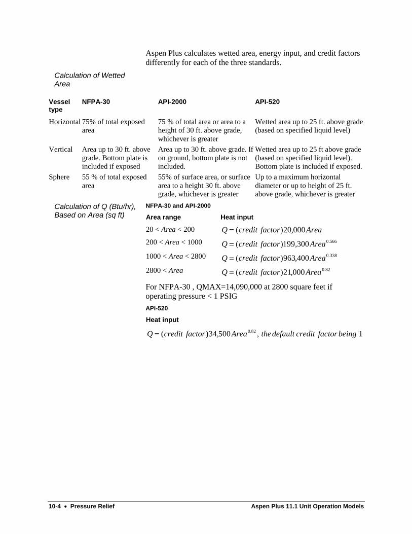
10-4 • Pressure Relief Aspen Plus 11.1 Unit Operation Models
Aspen Plus calculates wetted area, energy input, and credit factorsdifferently for each of the three standards.
Vesseltype
NFPA-30 API-2000 API-520
Horizontal 75% of total exposedarea
75 % of total area or area to aheight of 30 ft. above grade,whichever is greater
Wetted area up to 25 ft. above grade(based on specified liquid level)
Vertical Area up to 30 ft. abovegrade. Bottom plate isincluded if exposed
Area up to 30 ft. above grade. Ifon ground, bottom plate is notincluded.
Wetted area up to 25 ft above grade(based on specified liquid level).Bottom plate is included if exposed.
Sphere 55 % of total exposedarea
55% of surface area, or surfacearea to a height 30 ft. abovegrade, whichever is greater
Up to a maximum horizontaldiameter or up to height of 25 ft.above grade, whichever is greater
NFPA-30 and API-2000
Area range Heat input
20 < Area < 200 Q credit factor Area= ( ) ,20 000
200 < Area < 1000 Q credit factor Area= ( ) , .199 300 0 566
1000 < Area < 2800 Q credit factor Area= ( ) , .963 400 0 338
2800 < Area Q credit factor Area= ( ) , .21 000 0 82
For NFPA-30 , QMAX=14,090,000 at 2800 square feet ifoperating pressure < 1 PSIG
API-520
Heat input
Q credit factor Area thedefault credit factor being= ( ) , ,.34 500 10 82
Calculation of WettedArea
Calculation of Q (Btu/hr),Based on Area (sq ft)

Aspen Plus 11.1 Unit Operation Models Pressure Relief • 10-5
Type NFPA-30 API-2000 API-520
Insulation only .3 F=K(1660-TF)/21,000t
You must specify F
Same as API-2000
Drainage only .5
(Area > 200 sq. ft.)
1. Not defined
Water and drainage .3 1. Not defined
Water, insulation, anddrainage
.15
(Area > 200 sq. ft.)
NSUL Not defined
Insulation and drainage .15
(Area > 200 sq. ft.)
Not defined Not defined
Drainage and promptfire fighting effort
No credit Not defined 0.6*INSUL
Portable No credit factorsallowed
Not defined Not defined
This scenario is similar to the fire exposure scenario, except it canmodel any energy input. Aspen Plus can compute the energy inputfor this scenario in three ways depending on whether you specify:
• A constant duty
• A duty profile
• An area for heat transfer, a heat transfer coefficient, and asource fluid temperature
This scenario is a dynamic scenario and is typically used forelectrical heaters and other energy sources.
Use this scenario to find the flow rate through a specified reliefsystem at the specified composition. For this scenario, you mustenter your own :
• Relief rate
• Piping description
• Feed stream composition
• Feed stream condition
Use this scenario to find the flow rate through a valve, given thecomposition and condition at the entrance to the valve. This is thesimplest scenario. It is similar to the steady state flow rating ofrelief system scenario, except no piping is allowed.
Calculation of CreditFactors
Dynamic Run withSpecified Heat Flux intoVessel
Steady State Flow Ratingof Relief System
Steady State Flow Ratingof Relief Valve

10-6 • Pressure Relief Aspen Plus 11.1 Unit Operation Models
Pres-Relief allows two types of runs:
• Code capacity
• Actual capacity
The primary purpose of the code capacity run is to ensure that thecapacity of the relief system, rated as required by code, exceeds themaximum capacity dictated by the scenario. The maximumpressure reached during the relief event must be less than the codeallowable accumulation. The Code Capacity run includes the:
• ASME valve rating factor of .90
• Valve flow coefficient
• A combination coefficient
The combination coefficient is only included if a rupture disk/reliefvalve combination is being designed. Typical combinationcoefficients for NBBI certified combinations are close to 1.00. Ifthe combination is not certified, the ASME code requires acombination coefficient of .90. The primary purpose of the actualcapacity run is to provide the best estimate of the actual flowthrough the system. Design of downstream equipment (other thanthe tail pipe) is one example why you might need this information.The actual capacity run contains the valve flow coefficient, but notthe ASME valve rating factor of .90 or the combination coefficient.
For the steady-state scenarios, you must specify the compositionand conditions (two of temperature, pressure, and vapor fraction)of the feed stream. You can do this on the Setup Streams sheet intwo ways:
• Reference an Aspen Plus stream
• Give the composition and conditions of the stream as input toPres-Relief
For the dynamic scenarios, you must specify the composition andthe conditions in the vessel at the beginning of the pressure reliefcalculations. Do this by referencing an Aspen Plus stream, or byspecifying the composition and two of temperature, pressure, andvapor fraction on the Setup Vessel Contents sheet. As with thesteady-state scenarios, you may reference an Aspen Plus stream orgive the composition and conditions as input to Pres-Relief. Whenvapor fraction is not specified, you may also specify:
• Initial liquid fill fraction (fillage) of the vessel
• Pad-gas pressure and Component ID
Only two of temperature, pressure, and vapor fraction can bespecified or referenced from a stream.
Compliance withCodes
Stream and VesselCompositions andConditions
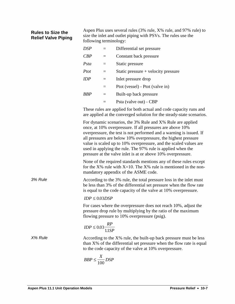
Aspen Plus 11.1 Unit Operation Models Pressure Relief • 10-7
Aspen Plus uses several rules (3% rule, X% rule, and 97% rule) tosize the inlet and outlet piping with PSVs. The rules use thefollowing terminology:
DSP = Differential set pressure
CBP = Constant back pressure
Psta = Static pressure
Ptot = Static pressure + velocity pressure
IDP = Inlet pressure drop
= Ptot (vessel) - Ptot (valve in)
BBP = Built-up back pressure
= Psta (valve out) - CBP
These rules are applied for both actual and code capacity runs andare applied at the converged solution for the steady-state scenarios.
For dynamic scenarios, the 3% Rule and X% Rule are appliedonce, at 10% overpressure. If all pressures are above 10%overpressure, the test is not performed and a warning is issued. Ifall pressures are below 10% overpressure, the highest pressurevalue is scaled up to 10% overpressure, and the scaled values areused in applying the rule. The 97% rule is applied when thepressure at the valve inlet is at or above 10% overpressure.
None of the required standards mentions any of these rules exceptfor the X% rule with X=10. The X% rule is mentioned in the non-mandatory appendix of the ASME code.
According to the 3% rule, the total pressure loss in the inlet mustbe less than 3% of the differential set pressure when the flow rateis equal to the code capacity of the valve at 10% overpressure.
IDP DSP≤ 0 03.
For cases where the overpressure does not reach 10%, adjust thepressure drop rule by multiplying by the ratio of the maximumflowing pressure to 10% overpressure (psig).
IDPRP
SP≤ 0 03
11.
.
According to the X% rule, the built-up back pressure must be lessthan X% of the differential set pressure when the flow rate is equalto the code capacity of the valve at 10% overpressure.
BBPX
DSP≤100
Rules to Size theRelief Valve Piping
3% Rule
X% Rule

10-8 • Pressure Relief Aspen Plus 11.1 Unit Operation Models
For cases where the overpressure does not reach 10% adjust thepressure drop rule by multiplying by the square of the ratio of themaximum flowing pressure to 10% overpressure (psig).
BBPX RP
PS≤
100 11
2
.
According to the 97% rule, 97% of the differential set pressuremust be available across the valve anytime the over pressure isequal to or above 10% with a flow through the valve based on codecapacity.
RP CBP IDP BBP DSP− − − ≥ 0 97.
For cases where the overpressure does not reach 10%, apply therule at peak overpressure.
For standard spring loaded valves or pop action pilot valves withunbalanced pilots vented to the discharge:
The differential set pressure is the set pressure minus the constantback pressure.
DSP SP CBP= −Size the inlet piping using the 3% rule.
Size the outlet piping using the 97% rule.-Or-Size the outlet piping with the X% rule using X = 10.
For balanced bellows spring loaded valves:
The differential set pressure is the set pressure.
DSP SP=Size the inlet piping using the 3% rule.
Size the outlet piping with the X% rule using X = 30.
For modulating pilot operated valves with balanced pilots orpilots vented to atmosphere:
The differential set pressure is the set pressure.
DSP SP=You can use the scenario required flow rather than the valvecapacity for pressure drop calculations as an option. This caneasily be simulated by changing the input orifice area until theoverpressure reaches 10%.
There is no inlet pressure drop rule.
Size the outlet piping with the X% rule using X = 50.
97% Rule
Recommendations forSpecific Valve Types

Aspen Plus 11.1 Unit Operation Models Pressure Relief • 10-9
If the protected vessel is a vertical, horizontal, API, spherical , oruser-specified tank, you may model it with or without reactions.Specify the reactions by giving the Reactions ID on the SetupReactions sheet.
The venting system consists of:
• A vessel neck
• One or two sections of inlet pipe
• The relief device itself
• One or two sections of tail pipe
In a simulation, the system being modeled may consist of an inletpipe without a relief device, or a relief device connected to thevessel without an inlet pipe. The tail pipe is optional.
Pres-Relief can model the following types of relief devices:
• Safety relief valves (PSVs; both liquid and gas/2-phase)
• Rupture disks (PSDs)
• Emergency relief valves (ERVs)
• SRV/rupture disk combinations
• Open vent pipes
Internal tables (accessed from the ReliefDevice SafetyValve sheet)contain several standard commercially available valves, along withall the mechanical specifications and certified coefficients neededin the relief calculations. You may choose one valve from thetables, or enter your own valve specifications and coefficients.
For liquid service valves, you must also specify the full-liftoverpressure. This allows Aspen Plus to simulate some of the olderstyle valves which do not achieve full lift until 25% overpressure isreached.
For gas/2-phase service valves, you must also specify the averageopening and closing factors. The valve does not open until thepressure drop across the valve reaches (opening factor * Dif-Setp).The valve closes when the pressure drop across it reaches (closingfactor * Dif-Setp).
In an actual capacity run, the rupture disk is modeled as a bit ofresistance using the pipe model. The default value of L/D is 8 for arupture disk with a diameter of 2 inches or less and 15 if thediameter is greater than 2 inches. You can override the default byspecifying a value on the Relief Device Rupture Disk sheet.
In the code capacity run, the rupture disk is modeled as an idealnozzle with a certified discharge coefficient. If no certifieddischarge coefficient is available, a value of 0.62 is suggested.
Reactions
Relief System
Relief Devices
10-10 • Pressure Relief Aspen Plus 11.1 Unit Operation Models
In a code capacity run in combination with a safety relief valve, theresistance of the rupture disk is modeled by the combinationcoefficient in the valve model.
The emergency relief vent is modeled as a nozzle. A de-ratingfactor of 0.9 is used in a code capacity run.
The inlet piping system can be made of one of the following:
• One pipe section
• Two sections of pipe plus a vessel neck, all with differentdiameters
The tail pipe can be made of one section of pipe or of two sectionsof pipe with different diameters.
For each pipe section, specify:
• Pipe diameter
• Length
• Elevation
• Whether the pipes are screwed together or held together withflanges or welds
If pipes of different diameters are used, reducer and expanderresistance coefficients ("K" factors) can be specified. Aspen Plususes the equation K =4*fr*(L/D) to convert from resistancecoefficients to equivalent L/D, where the term "fr" is the frictionfactor. Optional information for each section consists of thenumber of 90 degree elbows, straight tees, branched tees, gatevalves, butterfly valves, transflo valves, and control valves. Youcan add other fittings not listed by specifying the L/D value.Aspen Plus calculates a total equivalent L/D before modeling thepipe section.
You may also specify:
• Ambient temperature at the inlet and outlet of the pipe
• A heat transfer coefficient to exchange heat with the pipecontents
While modeling the pipe section, Aspen Plus detects the chokedcondition in the pipe by keeping track of the Mach Number asintegration down the pipe proceeds. If the Mach Number goesabove 1.0, integration is stopped and a flag is returned to indicatethat the pipe choked.
Pipeline pressure drop modeling can work in two ways. You mayspecify one of the following:
• Rigorous flashes are to be done at each step in the integration
• A flash table is used during pipe integration
Piping System

Aspen Plus 11.1 Unit Operation Models Pressure Relief • 10-11
If you request a table, specify the number of temperature andpressure points in the table. At each temperature-pressure pair,Aspen Plus performs a flash and calculates all necessary properties(density, viscosity, surface tension, and so on). As integrationproceeds, Aspen Plus interpolates in this table to get the necessaryproperties. If properties outside the table are needed, a rigorousflash is performed at that point. In general, the pipe integrationproceeds faster if the flash table is used. Several correlations areavailable, depending on the pipe inclination. The default methodfor all inclinations (holdup and frictional pressure loss) is Beggsand Brill. Other available options are:
• Darcy
• Lockhart-Martinelli
• Dukler for frictional loss
• Lockhart-Martinelli, Slack, and Flanigan for holdup

10-12 • Pressure Relief Aspen Plus 11.1 Unit Operation Models
Pres-Relief includes several customizable tables that list theavailable options for pipes, general purpose valves, safety reliefvalves, emergency relief vents, and rupture disks. You can modifythe tables by changing data files. Then process the files throughModelManager Table Building System (MMTBS).
Pres-Relief includes a table of actual diameters for several steelpipe schedules. Use this table when choosing the piping for theinlet and tail pipes. You can modify this table by including morepipe materials and/or schedules. The table is organized as follows:
first material of constructionnumber of typesfirst typenumber of diametersnominal diameter actual diameternominal diameter actual diameter..second typenumber of diametersnominal diameter actual diameternominal diameter actual diameter..second material of constructionnumber of typesfirst typenumber of diametersnominal diameter actual diameternominal diameter actual diameter..second typenumber of diametersnominal diameter actual diameternominal diameter actual diameter..
Data Tables for Pipesand Relief Devices
Pipes
Aspen Plus 11.1 Unit Operation Models Pressure Relief • 10-13
For general-purpose valves in the inlet or tail pipes, Pres-Reliefincludes a table of various manufacturers’ valves from 1 inch to 10inches. The valves include:
• Durco Plug
• Tufline Plug
• Jamesbury Ball
• AGCO Selector
• KTM Ball (L-Port and T-Port)
For each manufacturer, the table contains:
• Valve type (for example., L-Port or T-Port)
• Nominal diameter
• Port area
• Flow coefficient
The table is organized as follows:
first manufacturernumber of typesfirst typenumber of diametersnominal diameter port area flow coeffnominal diameter port area flow coeff..second typenumber of diametersnominal diameter port area flow coeffnominal diameter port area flow coeff..
General-Purpose Valves

10-14 • Pressure Relief Aspen Plus 11.1 Unit Operation Models
Pres-Relief includes a table of manufacturers’ safety relief valves.It contains valves for liquid and gas/2-phase service. For eachvalve, the table contains:
• Service
• Type
• Manufacturer
• Series, size (for example, 3L4)
• Throat diameter
• Inlet diameter
• Outlet diameter
• Discharge coefficient
• Overpressure factor (for liquid service valves)
The table is organized as follows:
Service (Liquid, Gas, or 2-phase)number of typesfirst typenumber of manufacturersfirst manufacturernumber of seriesfirst seriesnumber of sizesfirst sizenumber of throat diametersthroat diam inlet diam outlet diam dischg coeff over pr factorthroat diam inlet diam outlet diam dischg coeff over pr factor..throat diam inlet diam outlet diam dischg coeff over pr factorthroat diam inlet diam outlet diam dischg coeff over pr factor
Safety Relief Valves
Aspen Plus 11.1 Unit Operation Models Pressure Relief • 10-15
This table contains:
• Nominal diameter
• Effective diameter
• Allowed setpoint for several Protectoseal and Groth emergencyrelief vents
You must specify an over-pressure factor. The table is organized asfollows:
first manufacturer# of typesfirst type# of nominal diametersnominal diameter effective diameter allowed setpointnominal diameter effective diameter allowed setpoint..
This table contains manufacturers’ information on rupture disks.Each entry contains:
• A manufacturer
• Type
• Nominal diameter
• Actual diameter
• Discharge coefficient
The table is organized as follows:
first manufacturernumber of typesfirst typenumber of nominal diametersfirst nominal diam actual diam discharge coeffsecond nominal diam actual diam discharge coeff..
If a relief valve is too large for a given application, valve cyclingmay occur. In this situation, the pressure in the vessel builds up toa point where the valve opens, but then closes almost immediatelybecause enough material is released to lower the vessel pressurebelow the closing pressure. In some simulations, the valve mayopen and close several times per second. The simulation may runfor a long time, just opening and closing the valve over and over.
To stop such a simulation, you can specify whether or not to stopcycling, and how many openings and closings of the valve areallowed in a specified amount of time.
Emergency Relief Vents
Rupture Disks
Valve Cycling

10-16 • Pressure Relief Aspen Plus 11.1 Unit Operation Models
You must enter vessel geometry for the dynamic scenarios. Youcan choose one of the following vessel types:
• Vertical Vessel
• Horizontal Vessel
• API Tank
• Sphere
• Heat exchanger shell
• Vessel jacket
• User-specified
If you choose user-specified, you must specify surface area andvolume. Surface area is also required for vessel jacket. MaximumAllowable Working Pressure (MAWP) with correspondingtemperature is required for all vessel types. Some vessel typesrequire diameter, length, and volume of internals.
If you choose vertical vessel, horizontal vessel, or API tank,choose one of these head types:
• Flanged and dished
• Ellipsoidal
• User-specified
If you choose user-specified head type, you must specify the areaand volume of a head.
If the protected vessel is a sphere, you must specify:
• Diameter
• MAWP with corresponding temperature
• Volume of internals
If the protected vessel is a heat exchanger shell, in addition to theitems specified for a vertical vessel you must also specify whetherthe vessel is mounted vertically or horizontally.
If the protected vessel is a vessel jacket, you must specify:
• MAWP with corresponding temperature
• Volume of internals
• Jacket volume
If the protected vessel is user-specified, you must specify:
• Volume
• Area
• MAWP with corresponding temperature
• Volume of internals
Vessel Types
Vertical Vessel,Horizontal Vessel, andAPI Tank
Sphere
Heat Exchanger Shell
Vessel Jacket
User-Specified

Aspen Plus 11.1 Unit Operation Models Pressure Relief • 10-17
The following disengagement options are available:
Option Description
Homogeneous Vapor fraction leaving vessel is the same as vaporfraction in vessel
All-vapor All vapor leaving vessel
All-liquid All liquid leaving vessel
Bubbly DIERS bubbly model
Churn-turbulent DIERS churn-turbulent model
User-specified Homogeneous venting until vessel vapor fractionreaches the user-specified value, then all vapor venting
For the bubbly and churn-turbulent methods, Aspen Plus uses theDIERS "switch-point" calculations to compute the point at whichtotal vapor-liquid disengagement occurs. Use the bubbly andchurn-turbulent models only for vertical or API tanks.
For dynamic scenarios, stop criteria need to be specified whichwill terminate the simulation. You must:
• Select a specification type
• Enter a value for the specification at which the simulation willstop
• Select a component and substream for component-relatedspecification types
• Specify which approach direction (above or below) to use instopping the simulation
You may select from the following specification types:
• Simulation time
• Vapor fraction in the vessel
• Mole fraction of a specified component
• Mass fraction of a specified component
• Conversion of a specified component
• Total moles or moles of a specified component
• Total mass or mass of a specified component
• Vessel temperature
• Vessel pressure
• Vent mole flow rate or mole flow rate of a component
• Vent mass flow rate or mass flow rate of a component
DisengagementModels
Stop Criteria
10-18 • Pressure Relief Aspen Plus 11.1 Unit Operation Models
You must also select the location of the stop criteria specification.You may select from the following locations:
• Vessel
• Relief vent system
• Accumulator
Certain restrictions apply depending on the location selected.
When location = vessel, mole and mass flow rate are not allowed.
When location = vent accumulator, only the followingspecifications are allowed:
• Mass fraction of a specified component
• Mole fraction of a specified component
• Total moles of a specified component
• Total mass of a specified component
When location = vent, only the flowing specifications are allowed
• Mass fraction of a specified component
• Mole fraction of a specified component
• Vent molar flow rate
• Vent mass flow rate
The problem to be solved is:
Given the initial conditions in the vessel, a description of thepressure relief system, and the heat flow into the vessel, calculatethe flow rate through the pressure relief system and determine ifthe pressure relief system meets code requirements.
The problem is solved as outlined below. This algorithm is for theHeat-Input and Fire Scenarios.
1 Given the heat input to the vessel, solve the energy balance andflash equations along with the reaction equations for the vesselat the present time step. If any of the termination criteria aremet, go to Step 6. The options for specifying terminationcriteria include:
• Time for scenario exceeded
• Specified vapor fraction reached
• Vessel contents have reached specified value
• Pressure in the vessel is greater than the maximum allowed
2 If the pressure in the vessel is less than the device openingpressure, increment time and go to Step 1.
3 Calculate the maximum flow rate possible through the pressurerelief system. This value is calculated by finding the smallest
Solution Procedurefor DynamicScenarios

Aspen Plus 11.1 Unit Operation Models Pressure Relief • 10-19
diameter of any pipe or valve in the system, and calculating thesonic velocity through that diameter.
4 Calculate the pressure at the end of the vessel neck, after eachsection of the inlet pipe, after the pressure relief device, andafter each section of the tail pipe based on the current flowestimate. If the pressure at the end of any section is less thanthe user-specified discharge pressure, it is not necessary to dothe calculations for the next section.
5 If the pressure at the end of the pressure relief system is withintolerance of the user-specified discharge pressure, incrementtime and go to Step 1.
Otherwise, calculate a new guess for the flow through the reliefsystem and go to Step 4.
6 Given the flow at any time, check where the choke point is. Ifthe choke point is not at the pressure relief valve, the system isunacceptable. Check if any applicable codes are violated. If so,the system is unacceptable.
The next sections describe pipe flow and nozzle flow equations.
This is the general differential equation for flow through a constantdiameter pipe:
υ υ υυ
dp G d fD
dL g dL+ +
+ =2
2
42
0sinΦ(1)
Where:
υ = Specific volume of stream
p = Static (flowing) pressure of stream
G = Mass flow rate per unit area
f = Friction factor
D = Inside diameter of pipe
L = Equivalent pipe length
g = Acceleration due to gravity
sin Φ = Vertical rise/equivalent pipe length
Φ represents the physical angle of the pipe with respect to thehorizontal only if the equivalent pipe length is the same as thephysical flow path length (that is, only pipe, no fittings or otherresistances). The potential energy term in the equation assumesthat the vertical elevation is distributed evenly along the entireequivalent length.
Flow Equations
Pipe Flow
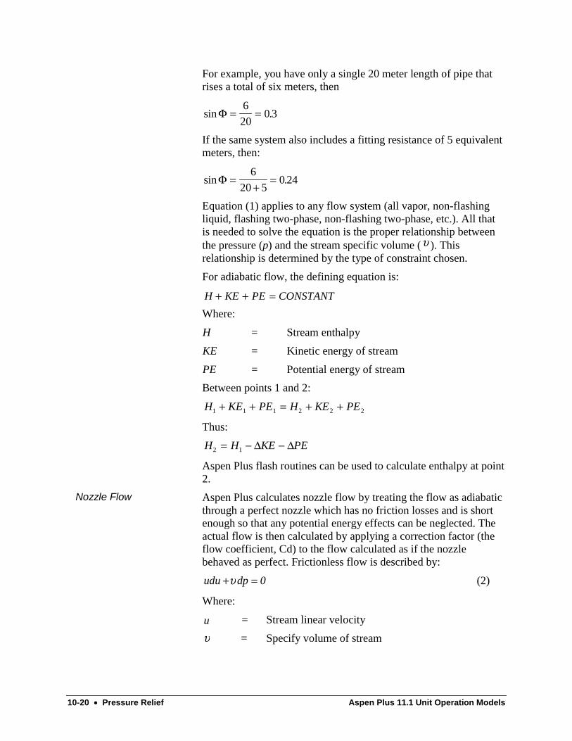
10-20 • Pressure Relief Aspen Plus 11.1 Unit Operation Models
For example, you have only a single 20 meter length of pipe thatrises a total of six meters, then
sin .Φ = =6
200 3
If the same system also includes a fitting resistance of 5 equivalentmeters, then:
sin .Φ =+
=6
20 50 24
Equation (1) applies to any flow system (all vapor, non-flashingliquid, flashing two-phase, non-flashing two-phase, etc.). All thatis needed to solve the equation is the proper relationship betweenthe pressure (p) and the stream specific volume (υ ). Thisrelationship is determined by the type of constraint chosen.
For adiabatic flow, the defining equation is:
H KE PE CONSTANT+ + =Where:
H = Stream enthalpy
KE = Kinetic energy of stream
PE = Potential energy of stream
Between points 1 and 2:
H KE PE H KE PE1 1 1 2 2 2+ + = + +
Thus:
H H KE PE2 1= − −∆ ∆
Aspen Plus flash routines can be used to calculate enthalpy at point2.
Aspen Plus calculates nozzle flow by treating the flow as adiabaticthrough a perfect nozzle which has no friction losses and is shortenough so that any potential energy effects can be neglected. Theactual flow is then calculated by applying a correction factor (theflow coefficient, Cd) to the flow calculated as if the nozzlebehaved as perfect. Frictionless flow is described by:
udu dp+ =υ 0 (2)
Where:
u = Stream linear velocity
υ = Specify volume of stream
Nozzle Flow
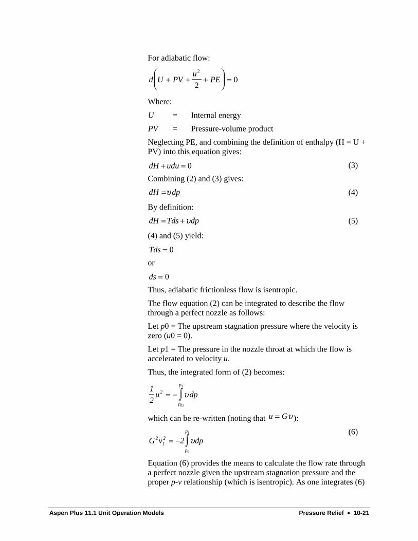
Aspen Plus 11.1 Unit Operation Models Pressure Relief • 10-21
For adiabatic flow:
d U PVu
PE+ + +
=
2
20
Where:
U = Internal energy
PV = Pressure-volume product
Neglecting PE, and combining the definition of enthalpy (H = U +PV) into this equation gives:
dH udu+ = 0 (3)
Combining (2) and (3) gives:
dH dp=υ (4)
By definition:
dH Tds dp= +υ (5)
(4) and (5) yield:
Tds = 0
or
ds = 0
Thus, adiabatic frictionless flow is isentropic.
The flow equation (2) can be integrated to describe the flowthrough a perfect nozzle as follows:
Let p0 = The upstream stagnation pressure where the velocity iszero (u0 = 0).
Let p1 = The pressure in the nozzle throat at which the flow isaccelerated to velocity u.
Thus, the integrated form of (2) becomes:
1
22
01
1
u dpp
p
= − ∫υ
which can be re-written (noting that u G= υ ):
G v dpp
p
212 2
0
1
= − ∫υ(6)
Equation (6) provides the means to calculate the flow rate througha perfect nozzle given the upstream stagnation pressure and theproper p-v relationship (which is isentropic). As one integrates (6)
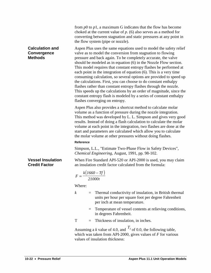
10-22 • Pressure Relief Aspen Plus 11.1 Unit Operation Models
from p0 to p1, a maximum G indicates that the flow has becomechoked at the current value of p. (6) also serves as a method forconverting between stagnation and static pressures at any point inthe flow system (pipe or nozzle).
Aspen Plus uses the same equations used to model the safety reliefvalve as to model the conversion from stagnation to flowingpressure and back again. To be completely accurate, the valveshould be modeled as in equation (6) in the Nozzle Flow section.This model requires that constant entropy flashes be performed ateach point in the integration of equation (6). This is a very timeconsuming calculation, so several options are provided to speed upthe calculations. First, you can choose to do constant enthalpyflashes rather than constant entropy flashes through the nozzle.This speeds up the calculations by an order of magnitude, since theconstant entropy flash is modeled by a series of constant enthalpyflashes converging on entropy.
Aspen Plus also provides a shortcut method to calculate molarvolume as a function of pressure during the nozzle integration.This method was developed by L. L. Simpson and gives very goodresults. Instead of doing a flash calculation to calculate the molarvolume at each point in the integration, two flashes are done at thestart and parameters are calculated which allow you to calculatethe molar volume at other pressures without doing flashes.
Reference
Simpson, L.L., "Estimate Two-Phase Flow in Safety Devices",Chemical Engineering, August, 1991, pp. 98-102.
When Fire Standard API-520 or API-2000 is used, you may claiman insulation credit factor calculated from the formula:
( )F
k Tf
t=
−1660
21000
Where:
k = Thermal conductivity of insulation, in British thermalunits per hour per square foot per degree Fahrenheitper inch at mean temperature.
= Temperature of vessel contents at relieving conditions,in degrees Fahrenheit.
T = Thickness of insulation, in inches.
Assuming a k value of 4.0, and Tf of 0.0, the following table,
which was taken from API-2000, gives values of F for variousvalues of insulation thickness:
Calculation andConvergenceMethods
Vessel InsulationCredit Factor

Aspen Plus 11.1 Unit Operation Models Pressure Relief • 10-23
Insulation thickness (t) F Factor
6 inches (152 millimeters) 0.05
8 inches (203 millimeters) 0.037
10 inches (254 millimeters) 0.03
12 inches (305 millimeters) or more 0.025
"Sizing, Selection, and Installation Of Pressure-Relieving Devicesin Refineries" Part I - Sizing and Selection, API RecommendedPractice 520, American Petroleum Institute, 1220 L StreetNorthwest, Washington, D.C. 20005.
"Venting Atmospheric and Low Pressure Storage Tanks", (Non-refrigerated and Refrigerated), API Standard 2000, AmericanPetroleum Institute, 1220 L Street Northwest, Washington, D.C.20005.
Additional Reading

10-24 • Pressure Relief Aspen Plus 11.1 Unit Operation Models

Aspen Plus 11.1 Unit Operation Models Advanced Distillation Features • A-1
A P P E N D I X A
Advanced Distillation Features
This appendix contains information applicable to several of thedistillation column models in Aspen Plus. The topics are:
• Sizing and Rating for Trays and Packing
• Column Targeting
A-2 • Advanced Distillation Features Aspen Plus 11.1 Unit Operation Models
Sizing and Rating for Trays andPackings: OverviewAspen Plus has extensive capabilities to size, rate, and performpressure drop calculations for trayed and packed columns. Use thefollowing Tray/Packing forms to enter specifications:
• TraySizing
• TrayRating
• PackSizing
• PackRating
These capabilities are available in the following column unitoperation models:
• RadFrac
• MultiFrac
• PetroFrac
You can choose from the following five commonly-used traytypes:
• Bubble caps
• Sieve
• Glitsch Ballast®
• Koch Flexitray®
• Nutter Float Valve
Aspen Plus can model a variety of random packings. You can alsouse any of the following types of structured packings:
• Goodloe®
• Glitsch Grid®
• Norton Intalox Structured Packing
• Sulzer BX, CY, Mellapak, and Kerapak
• Koch Flexipac, Flexeramic, Flexigrid
• Raschig Super-Pak and Ralu-Pak
For sizing and rating calculations, Aspen Plus divides a columninto sections. Each section can have a different tray type, packingtype, and diameter. The tray details can vary from section tosection. A column can have an unlimited number of sections. Inaddition, you can size and rate the same section with differenttypes of trays and packings.
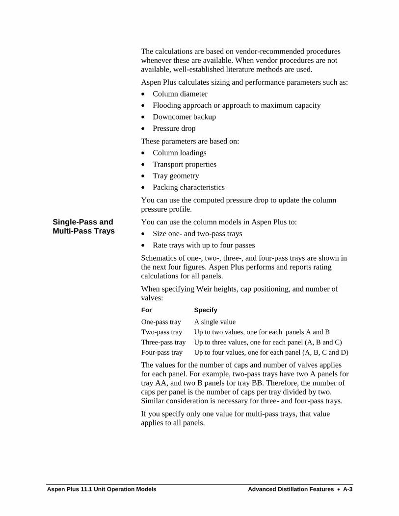
Aspen Plus 11.1 Unit Operation Models Advanced Distillation Features • A-3
The calculations are based on vendor-recommended procedureswhenever these are available. When vendor procedures are notavailable, well-established literature methods are used.
Aspen Plus calculates sizing and performance parameters such as:
• Column diameter
• Flooding approach or approach to maximum capacity
• Downcomer backup
• Pressure drop
These parameters are based on:
• Column loadings
• Transport properties
• Tray geometry
• Packing characteristics
You can use the computed pressure drop to update the columnpressure profile.
You can use the column models in Aspen Plus to:
• Size one- and two-pass trays
• Rate trays with up to four passes
Schematics of one-, two-, three-, and four-pass trays are shown inthe next four figures. Aspen Plus performs and reports ratingcalculations for all panels.
When specifying Weir heights, cap positioning, and number ofvalves:
For Specify
One-pass tray A single value
Two-pass tray Up to two values, one for each panels A and B
Three-pass tray Up to three values, one for each panel (A, B and C)
Four-pass tray Up to four values, one for each panel (A, B, C and D)
The values for the number of caps and number of valves appliesfor each panel. For example, two-pass trays have two A panels fortray AA, and two B panels for tray BB. Therefore, the number ofcaps per panel is the number of caps per tray divided by two.Similar consideration is necessary for three- and four-pass trays.
If you specify only one value for multi-pass trays, that valueapplies to all panels.
Single-Pass andMulti-Pass Trays

A-4 • Advanced Distillation Features Aspen Plus 11.1 Unit Operation Models
When specifying downcomer clearance and width:
For Specify
One-pass tray A single value for the side downcomer
Two-pass tray Up to two values, one for the side downcomer, one forthe center downcomer
Three-pass tray Up to two values, one for the side downcomer, one forthe off-center downcomer
Four-pass tray Up to three values: one for the side downcomer, onefor the center downcomer, and one for the off-centerdowncomer
DC-WTOPWEIR-HT
DC-HTDC-WBOT
Ou
tlet
Wei
r L
eng
th
Column Diameter
DC-CLEAR
A One-Pass Tray
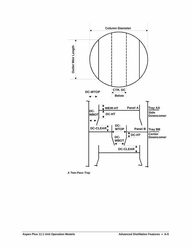
Aspen Plus 11.1 Unit Operation Models Advanced Distillation Features • A-5
DC-WTOP
DC-CLEAR
DC-CLEAR
Panel A
Panel B
WEIR-HT
DC-HT
DC-HTDC-WBOT
DC-WBOT
Tray AASideDowncomer
Tray BB
CenterDowncomer
Below
CTR. DC
CTR. DC
~
~
~
~
~ ~
DC-WTOP
Column Diameter
Ou
tlet
Wei
r L
eng
th
A Two-Pass Tray
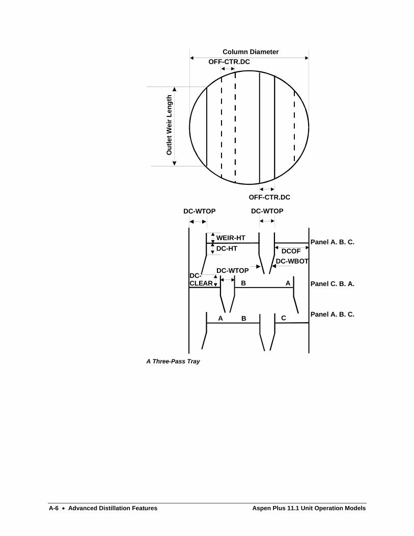
A-6 • Advanced Distillation Features Aspen Plus 11.1 Unit Operation Models
DC-WTOPDC-WBOT
DCOFPanel A. B. C.
Panel A. B. C.
Panel C. B. A.
BA C
DC-WTOP DC-WTOP
B A
OFF-CTR.DC
OFF-CTR.DC
WEIR-HT
DC-HT
DC-CLEAR
Column Diameter
Ou
tlet
Wei
r L
eng
th
A Three-Pass Tray
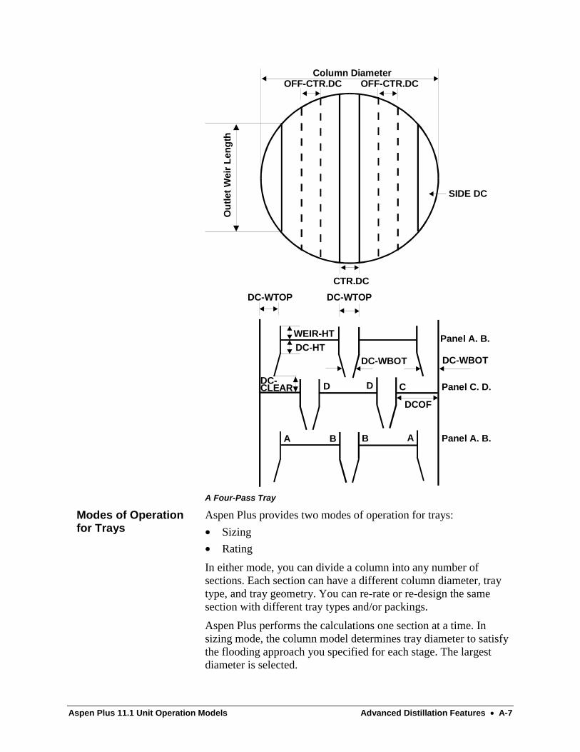
Aspen Plus 11.1 Unit Operation Models Advanced Distillation Features • A-7
OFF-CTR.DCOFF-CTR.DC
SIDE DC
CTR.DC
DC-WTOP DC-WTOP
WEIR-HTDC-HT
DC-WBOTDC-WBOT
Panel A. B.
Panel C. D.
Panel A. B.
DCOF
DC-CLEAR D D C
A AB B
Column Diameter
Ou
tlet
Wei
r L
eng
th
A Four-Pass Tray
Aspen Plus provides two modes of operation for trays:
• Sizing
• Rating
In either mode, you can divide a column into any number ofsections. Each section can have a different column diameter, traytype, and tray geometry. You can re-rate or re-design the samesection with different tray types and/or packings.
Aspen Plus performs the calculations one section at a time. Insizing mode, the column model determines tray diameter to satisfythe flooding approach you specified for each stage. The largestdiameter is selected.
Modes of Operationfor Trays

A-8 • Advanced Distillation Features Aspen Plus 11.1 Unit Operation Models
In rating mode, you specify the column section diameter and othertray details. For each stage, the column model calculates trayperformance and hydraulic information such as flooding approach,downcomer backup, and pressure drop.
For bubble caps and sieve trays, Aspen Plus provides twoprocedures for calculating the approach to flooding. The firstprocedure is based on the Fair method. The second uses the Glitschprocedure for ballast trays. This procedure de-rates the calculatedflooding approach by 15% for bubble caps and by 5% for sievetrays. All other hydraulic calculations are based on the Fair andBolles methods. You can also supply your own calculationprocedure:
= Specify On form
Flooding calculation method = USER TraySizing or TrayRating
Subroutine name UserSubroutines
For valve trays (Glitsch Ballast, Koch Flexitray, and Nutter FloatValve trays), Aspen Plus uses procedures from vendor designbulletins.
Two versions of vendor design bulletins are available for KochFlexitray:
• Bulletin 960
• Bulletin 960-1
You can use the Convergence form to specify which bulletin to usefor all TraySizing and TrayRating sections for a block. You canspecify which bulletin to use for each section. This specificationoverrides the block-wise specification. For valve type S, AO, andTO in the TrayRating sections, Aspen Plus always uses Bulletin960-1 internally, regardless of the block-wise specification. For allother cases, the default is Bulletin 960.
For Nutter Float Valve trays, two versions of curve fitting areprovided for curves in the vendor design bulletin:
• Aspen90
• Aspen96
Aspen96 is recommended. Use the Convergence form to specifywhich version to use.
Flooding Calculationsfor Trays

Aspen Plus 11.1 Unit Operation Models Advanced Distillation Features • A-9
RadFrac uses cap diameter only for tray type CAPS. Valid entriesare:
Cap Diameter Default Weir Height
Inches Millimeters Inches Millimeters
3 76.2 2.75 69.85
4 101.6 3.00 76.20
6 152.4 3.25 82.55
Use the cap diameter to retrieve cap characteristics based onstandard cap designs.
For columns with diameter The default is
Up to 48 in (1219.2 mm). 3 in (76.2 mm)
Greater than 48 in (1219.2 mm) 4 in (101.6 mm)
The following table lists standard cap designs:
Material Stainless Steel
Nominal Size, in 3 4 6
Cap
U.S. Standard gauge 16 16 16
OD, in 2.999 3.999 5.999
ID, in 2.875 3.875 5.875
Height overall, in 2.500 3.000 3.750
Number of slots 20 26 39
Type of slots Trapezoidal Trapezoidal Trapezoidal
Slot width, in
Bottom 0.333 0.333 0.333
Top 0.167 0.167 0.167
Slot height, in 1.000 1.250 1.500
Height shroud ring, in 0.250 0.250 0.250
Riser
U.S. Standard gauge 16 16 16
OD, in 1.999 2.624 3.999
ID, in 1.875 2.500 3.875
Material Stainless Steel
Nominal size, in 3 4 6
Standard heights, in
0.5-in skirt height 2.250 2.500 2.750
1.0-in skirt height 2.750 3.000 3.250
1.5-in skirt height 3.250 3.500 3.750
Riser-slot seal, in 0.500 0.500 0.500
Cap areas, in
Bubble Cap TrayLayout

A-10 • Advanced Distillation Features Aspen Plus 11.1 Unit Operation Models
Riser 2.65 4.80 11.68
Reversal 4.18 7.55 17.80
Annular 3.35 6.38 14.55
Slot 5.00 8.12 14.64
Cap 7.07 12.60 28.30
Area ratios
Reversal/riser 1.58 1.57 1.52
Annular/riser 1.26 1.33 1.25
Slot/riser 1.89 1.69 1.25
Slot/cap 0.71 0.65 0.52
Normally, RadFrac, MultiFrac, and PetroFrac treat the stages youenter as equilibrium stages. You must enter overall efficiency to:
• Convert the calculated pressure drop per tray to pressure dropper equilibrium stage
• Compute the column pressure drop
If you do not enter overall efficiency, these models assume 100%efficiency. If you specify Murphree or vaporization efficiency, youshould not enter overall efficiency. RadFrac, MultiFrac, andPetroFrac will treat the stages as actual trays.
Suggested values for Ballast trays are:
Service System Foaming Factor
Non-foaming systems 1.00
Fluorine systems 0.90
Moderate foamers, such as oilabsorbers, amine, and glycolregenerators
0.85
Heavy foamers, such as amine andglycol absorbers
0.73
Severe foamers, such as MEK units 0.60
Foam stable systems, such as causticregenerators
0.30
Suggested values for Flexitrays are:
Service System Foaming Factor
Depropanizers 0.85-0.95
Absorbers 0.85
Vacuum towers 0.85
Amine regenerators 0.85
Amine contactors 0.70-0.80
High pressure deethanizers 0.75-0.80
Glycol contactors 0.70-0.75
Pressure DropCalculations forTrays
Foaming Calculationsfor Trays
Aspen Plus 11.1 Unit Operation Models Advanced Distillation Features • A-11
Suggested values for Float valve trays are:
Service System Foaming Factor
Non foaming 1.00
Low foaming 0.90
Moderate foaming 0.75
High foaming 0.60
The calculations for packings are based on the height equivalent ofa theoretical plate (HETP). HETP=packed height/number ofstages. The HETP is required. You can provide it using one of thefollowing methods:
• Enter it directly on the PackSizing or PackRating forms
• Enter the packing height on the same form
Aspen Plus can handle a wide variety of packing types, includingdifferent sizes and materials from various vendors.
For random packings, the calculations require packing factors.Aspen Plus stores packing factors for the various sizes, materials,and vendors allowed in a databank. If you provide the followinginformation, Aspen Plus retrieves these packing factorsautomatically for calculations:
• Packing type
• Size
• Material
You may specify the vendor on the PackSizing or PackRatingform.
Is the vendorspecified? Aspen Plus uses
Yes The packing factor published by the vendor
No A value compiled from various literature sources
You can enter the packing factor directly to override the built-invalues. Aspen Plus uses the packing type to select the propercalculation procedure.
Literature Sources
Fair, J.R., et al., "Liquid-Gas Systems," Perry’s ChemicalEngineers’ Handbook, R.H. Perry and D. Green, ed., 6th ed. (NewYork: McGraw Hill, 1984).
Tower Packings, Bulletin No. 15 (Tokyo: Tokyo Special WireNetting Company).
Packed Columns
Packing Types andPacking Factors
A-12 • Advanced Distillation Features Aspen Plus 11.1 Unit Operation Models
The column models have two modes of operation for packing:
• Sizing
• Rating
In either mode, you can divide a column into any number ofsections. Each section can have different packings. You can re-rateor re-design the same section with different packings and/or traytypes. Aspen Plus performs the calculations one section at a time.
In sizing mode, Aspen Plus determines the column sectiondiameter from:
• The approach to the maximum capacity
• A design capacity factor you specify
You can impose a maximum pressure drop per unit height (ofpacking or per section) as an additional constraint. OnceAspen Plus has determined the column section diameter, it re-ratesthe stages in the section with the calculated diameter.
In rating mode, you specify the column diameter. Aspen Pluscalculates the approach to maximum capacity and pressure drop.
Aspen Plus provides several methods for maximum capacitycalculations. For random packings you can use:
Method For this type of packings
Mass Transfer, Ltd. (MTL) 1 MTL
Norton 2 Norton IMTP
Koch 3 Koch
Raschig 4 Raschig
Eckert All other random packings
For structured packings, Aspen Plus provides vendor proceduresfor each type. If you specify the maximum capacity factor,Aspen Plus bypasses the maximum capacity calculations.
The definition of approach to maximum capacity depends on thetype of packings.
For Norton IMTP and Intalox structured packings, approach tomaximum capacity refers to the fractional approach to themaximum efficient capacity. Efficient capacity is the operatingpoint at which efficiency of the packing deteriorates due to liquidentrainment. The efficient capacity is approximately 10 to 20%below the flood point.
For Sulzer structured packings (BX, CY, Kerapak, and Mellapak),approach to maximum capacity refers to the fractional approach tomaximum capacity. Maximum capacity is the operating point atwhich a pressure drop of 12 mbar/m (1.47 in-water/ft) of packing
Modes of Operationfor Packing
Maximum CapacityCalculations forPacking
Aspen Plus 11.1 Unit Operation Models Advanced Distillation Features • A-13
is obtained. At this condition, stable operation is possible, but thegas load is higher than that at which maximum separationefficiency is achieved.
The gas load corresponding to the maximum capacity is 5 to 10%below the flood point. Sulzer recommends a usual design rangebetween 0.5 and 0.8 for approach to flooding.
For Raschig random and structured packings, approach tomaximum capacity refers to the fractional approach to maximumcapacity. Maximum capacity is at the loading point.
For all other packings, approach to maximum capacity refers to thefractional approach to the flood point.
Because there are different definitions for approach to maximumcapacity, sizing results are not on the same basis for packings fromdifferent vendors, even when you use the same value for approachto maximum capacity. Direct performance comparison of packingsfrom different vendors is not recommended.
The capacity factor is:
CS VS V
L V
=−ρ
ρ ρ
Where:
CS = Capacity factor
VS = Superficial velocity of vapor to packing
ρV = Density of vapor to packing
ρ L = Density of liquid from packing
References
1 Cascade Mini-Ring Design Manual (Tokyo: Dodwell &Company, Ltd., 1984).
2 Intalox High-Performance Separation Systems, Bulletin IHP-1(Akron: Norton Company, 1987).
3 McNulty, K.J., "Hydraulic Model for Packed Tower Design."Paper presented at the American Institute of ChemicalEngineers Spring Meeting in Houston, 1993.
4 Billet, R., and Schultes, M., "Modeling of Packed TowerPerformance for Rectification, Absorption and Desorption inthe Total Capacity Range." Paper presented at the 3rd Korea-Japan Symposium On Sep. Tech., October 25-27, 1993 inSeoul, Korea.

A-14 • Advanced Distillation Features Aspen Plus 11.1 Unit Operation Models
For random packings, Aspen Plus provides several built-inmethods to compute the pressure drop.
Vendor Pressure drop method
MTL Vendor 1
Norton Vendor procedure 2,3,4
Koch Vendor procedure 5
Raschig Vendor procedure 6
Not specified Eckert GPDC 7, Norton GPDC 2,3,4, Prahl GPDC 8, TsaiGPDC 9
If you specify the vendor, Aspen Plus uses the vendor procedure. Ifyou do not specify the vendor, you can choose one of four differentpressure drop methods. If you do not specify a method, Aspen Plususes the Eckert generalized pressure drop correlation (GPDC).
For structured packings, vendor pressure drop correlations areavailable for all packings:
Packing type Pressure drop method
Goodloe Vendor procedure 10
Glitsch Grid Vendor procedure 11
Norton Intalox Structured Packings Vendor procedure 12
Sulzer BX, CY, Mellapak, and Kerapak Vendor procedure 13
Super-Pak and Ralu-Pak Vendor procedure 6
Koch Flexipac, Flexeramic, and Flexigrid Vendor procedure 14
References
1 Cascade Mini-Ring Design Manual (Tokyo: Dodwell &Company, Ltd., 1984).
2 Dolan, M.J. and Strigle, R.F., "Advances in DistillationColumn Design," CEP, Vol.76, No.11 (November 1980), pp.78-83.
3 Intalox High-Performance Separation Systems, Bulletin IHP-1(Akron: Norton Company, 1987).
4 Intalox Metal Tower Packing, Bulletin IM82 (Akron: NortonCompany, 1979).
5 McNulty, K.J., "Hydraulic Model for Packed Tower Design."Paper presented at the American Institute of ChemicalEngineers Spring Meeting in Houston, 1993.
6 Billet, R., and Schultes, M., "Modeling of Packed TowerPerformance for Rectification, Absorption and Desorption inthe Total Capacity Range" Paper presented as the 3rd Korea-Japan Symposium On Sep. Tech., October 25-27, 1993 inSeoul, Korea.
Pressure DropCalculations forPacking
Aspen Plus 11.1 Unit Operation Models Advanced Distillation Features • A-15
7 Fair, J.R. et al., "Liquid-Gas Systems," Perry’s ChemicalEngineers’ Handbook, R.H. Perry and D. Green, ed., 6th ed.(New York: McGraw Hill, 1984), pp. 18-22.
8 McNulty, K.J. and Hsieh, C.L., "Hydraulic Performance andEfficiency of Koch Flexipac Structured Packings." Paperpresented at American Institute of Chemical Engineers AnnualMeeting in Los Angeles, 1982.
9 Tsai, T.C., "Packed Tower Program Has Special Features," Oiland Gas Journal, Vol. 83 No. 35 (September, 1985), p. 77.
10 Goodloe, Bulletin 520A (Dallas: Glitsch, Inc., 1981).
11 Glitsch Grid-Grid/Ring Combination Bed, Bulletin No. 7070(Dallas: Glitsch, Inc., 1978).
12 Norton Company, private communication, 1992.
13 Spiegel, L. and Meier, W., "Correlations of the PerformanceCharacteristics of the Various Mellapak Types." Paperpresented at the 4th International Symposium of Distillationand Absorption, Brighton, England, 1987.
14 McNulty, K.J., "Hydraulic Model for Packed Tower Design."Paper presented at the American Institute of ChemicalEngineers Spring Meeting in Houston, 1993.
Aspen Plus performs liquid holdup calculations for both randomand structured packings. For Raschig packings, Aspen Plus usesthe vendor procedure is used. The required parameters are voidfraction and surface area. If you do not provide these parameters,Aspen Plus will retrieve them from the built-in databank.
For other packings, Aspen Plus uses the Stichlmair correlation.The Stichlmair correlation requires these parameters:
• Packing void fraction and surface area
• Three Stichlmair correlation constants
When Stichlmair correlation is used, Aspen Plus provides theseparameters for a variety of packings in the built-in packingdatabank. If these parameters are missing for a particular packing,Aspen Plus will not perform liquid holdup calculations for thatpacking.
You can also enter these parameters to provide missing values, orto override the databank values.
You can update the pressure profile using:
• Computed pressure drops for the rating mode of both trays andpackings
• The sizing mode of packings
Liquid HoldupCalculations forPacking
Pressure ProfileUpdate

A-16 • Advanced Distillation Features Aspen Plus 11.1 Unit Operation Models
If you choose to update the pressure profile, the column modelssolve the tray or packing calculation procedures simultaneouslywith the column-describing equations. For updating the pressureprofile during calculations check Update Section Pressure Profileon the following forms:
• TrayRating
• PackSizing
• PackRating
Also, you can fix the pressure at the top or bottom of the columnand you can specify this option on the above forms. The stagepressures become additional variables. Aspen Plus uses thepressure specifications given on the Pres-Profile form to:
• Initialize the column pressure profile
• Fix the pressure drop of stages for which the pressure profile isnot updated
Several physical properties that are not normally used for heat andmaterial balance calculations are required for column sizing andrating. These properties are:
• Liquid and vapor densities
• Liquid surface tension
• Liquid and vapor viscosities
The physical property method that you specify for a unit operationmodel must be able to provide the required properties. In addition,the physical property parameters needed to calculate the requiredproperties must be available for all components in the column. Seethe descriptions of properties in the Aspen Plus User Guide,Chapter 8, for details on specifying physical property methods anddetermining property parameter requirements.
Fair, J.R., et al., "Liquid-Gas Systems," Perry’s ChemicalEngineers’ Handbook, R.H. Perry and D. Green, ed. 6th ed., NewYork: McGraw Hill, 1984.
Ballast Tray Design Manual, Glitsch, Inc. Bulletin No. 4900, 3rd
ed. Dallas, 1980.
Smith, B.D., "Tray Hydraulics: Bubble Cap Trays" and "TrayHydraulics: Perforated Trays," Design of Equilibrium StageProcesses, New York: McGraw Hill, 1963, pp. 474-569.
Koch Flexitray Design Manual, Koch Engineering Co., Inc.Bulletin No. 90, Wichita.
Ballast Tray Design Manual, Glitsch, Inc. Bulletin No. 4900, 3rd
ed. Dallas, 1980.
Physical PropertyData Requirements
References

Aspen Plus 11.1 Unit Operation Models Advanced Distillation Features • A-17
Koch Flexitray Design Manual, Koch Engineering Co., Inc.Bulletin No. 90, Wichita.
Nutter Float Valve Design Manual, Tulsa: Nutter Engineering Co.,1976.
Stichlmair, J., et al., "General Model for Prediction of PressureDrop and Capacity of Countercurrent Gas/Liquid PackedColumns," Gas Separation and Purification, Vol. 3 (1989), p. 22.

A-18 • Advanced Distillation Features Aspen Plus 11.1 Unit Operation Models
Column TargetingThe Aspen Plus Column Targeting tool offers capabilities forthermal and hydraulic analysis of distillation columns. Duringdesign or retrofit analysis of a process, these capabilities can beexploited to identify the targets for appropriate columnmodifications in order to:
• Reduce utilities cost
• Improve energy efficiency
• Reduce capital investment (by improved driving forces)
• Facilitate column debottlenecking
These capabilities are available for the following distillationcolumn models:
• RadFrac
• MultiFrac
• PetroFrac
The thermal analysis capability is useful in identifying designtargets for improvements in energy consumption and efficiency.This capability is based on the concept of minimumthermodynamic condition for a distillation column. The minimumthermodynamic condition pertains to thermodynamically reversiblecolumn operation. In this condition, a distillation column wouldoperate at minimum reflux, with an infinite number of stages, andwith heaters and coolers placed at each stage with appropriate heatloads for the operating and equilibrium lines to coincide. In otherwords, the reboiling and condensing loads are distributed over thetemperature range of operation of the column. The stage-enthalpy(Stage-H) or temperature-enthalpy (T-H) profiles for such acolumn therefore represent the theoretical minimum heating andcooling requirements in the temperature range of separation. Theseprofiles are called the Column Grand Composite Curves (CGCCs).
The Aspen Plus Column Targeting tool generates the CGCCsbased on the Practical Near-Minimum Thermodynamic Condition(PNMTC) approximation (Dhole and Linnhoff). The enthalpiesused in plotting the CGCCs are calculated at a given stage of thecolumn by assuming that the equilibrium and operating linescoincide at this stage. This approximation takes into account thelosses or inefficiencies introduced through practicalities of columndesign (such as pressure drops, multiple side-products, sidestrippers, etc.), while preserving the meaning of the CGCC. Theequations for equilibrium and operating lines are solvedsimultaneously at each stage for designated light key and heavy
Column TargetingThermal Analysis
Aspen Plus 11.1 Unit Operation Models Advanced Distillation Features • A-19
key components. The Aspen Plus Column Targeting tool has abuilt-in capability to select light key and heavy key components foreach stage of the column.
The CGCCs are helpful in identifying the targets for potentialcolumn modifications. These modifications include:
• Feed location
• Reflux ratio modifications
• Feed conditioning (heating or cooling)
• Side condensing or reboiling
An additional capability is provided through exergy analysis. Theexergy profiles are plotted by calculating the exergy loss at eachstage of the column, taking into account all entering and leavingmaterial and heat streams. In general, the exergy loss profiles canbe used as a tool to examine the degradation of potential workavailability (irreversibility) in a distillation column due to:
• Momentum loss (pressure driving force)
• Thermal loss (temperature driving force)
• Chemical potential loss (mass transfer driving force)
The hydraulic analysis capability is useful in understanding howthe vapor and liquid flow rates in a distillation column comparewith the minimum (corresponding to the PNMTC) and maximum(corresponding to flooding) limits. For packed and tray columns,jet flooding controls the calculation of vapor flooding limits. Fortray columns, parameters such as downcomer backup control theliquid flooding limits. Hydraulic analysis can be used to identifyand eliminate column bottlenecks.
For RadFrac, MultiFrac, and PetroFrac, the column targetingthermal and hydraulic analysis capabilities can be activated byusing the corresponding option buttons on the Report PropertyOptions forms.
Method for selecting light and heavy key components for thePNMTC calculations has to be specified. The component K-valuesbased method is used as default.
To calculate the maximum vapor and liquid flow rates due toflooding, you must specify tray or packing rating information forthe entire column. In addition, you can specify allowable floodingfactors (as fraction of total flooding) for flooding limitcalculations. The allowable limit for vapor flooding can bespecified on the TrayRating | Design/Pdrop or PackRating |Design/Pdrop sheets. The allowable limit for liquid flooding (dueto downcomer backup) can be specified on the TrayRating |Downcomers sheet. The default values are 85% for the vapor
Column TargetingHydraulic Analysis
Specifications forColumn Targetingand HydraulicAnalysis

A-20 • Advanced Distillation Features Aspen Plus 11.1 Unit Operation Models
flooding limit and 50% for the liquid flooding limit. The liquidflooding limit specification is available only if the downcomergeometry is specified.
Results of the column targeting analysis depend strongly on theselection of light key and heavy key components. The Aspen PlusColumn Targeting tool provides the following four methods forjudicious selection of these key components:
Method Use When
User defined Allows you to specify the light key and heavy keycomponents.
Based oncomponent split-fractions
Selects the light key and heavy key componentson the basis of component split-fractions incolumn product streams. This method is bestsuited for sharp or near-sharp splits.
Based oncomponent K-values
Selects the light key and heavy key componentson the basis of component K-values. This methodis best suited for sloppy splits.
Based on columncompositionprofiles
Selects the light and heavy key components on thebasis of composition profiles. In principle, thismethod is similar to the K-value based method. Itis best suited for sloppy splits and it is, in general,inferior to the K-value based method.
These methods can be chosen for the distillation models on thefollowing sheets:
Model Form
RadFrac Report Targeting Options
MultiFrac Columns Report Targeting Options
PetroFrac Report Targeting Options
Strippers Report Targeting Options
The associated parameters for each method can be chosen on thefollowing sheets:
Model Form
RadFrac Report Targeting Specifications
MultiFrac Columns Report Targeting Specifications
PetroFrac Report Targeting Specifications
Strippers Report Targeting Specifications
This method allows the user to define column sections and lightkey and heavy key components for each section. If the sectionsdefined do not cover the entire column, extrapolations are used. Ifthe selection of key components is inconsistent with the separationin the column, the column targeting calculations are skipped. In
Selection of KeyComponents
Selection of KeyComponents: UserDefined
Aspen Plus 11.1 Unit Operation Models Advanced Distillation Features • A-21
both cases, appropriate warning messages are written to the controlpanel and to the history file.
We highly recommend that you run the simulation and inspect thecolumn split-fractions, composition profiles, and component K-values before using this method to designate key components.
In this method the column is divided into sections bounded by itsproduct streams. For each section, the key components are selectedbased on the component split-fractions in its bounding productstreams as:
Component Mole-Fraction
Component Split -Fraction
Designation
In the section bottom-product > Compositiontolerance
In the section top-product> Minimum split-fraction
Light key
In the section top-product > Compositiontolerance
In the section bottom-product > Minimum split-fraction
Heavy key
If there is more than one light key component for a column section,the heaviest of these components is selected as the light key.Similarly, in case of multiple heavy keys for a column section, thelightest is selected as the heavy key. These selections are madebased on the component K-values.
If light key and/or heavy key components cannot be selected for acolumn section, appropriate extrapolations are used. If theseextrapolations do not produce a meaningful selection, columntargeting calculations are skipped. In both cases, appropriatewarnings are written to the control panel and to the history file.
The default values for the parameters used in this method are:
Parameter Default Value
Minimum split-fraction 0.9
Composition tolerance 1e-6
K-value tolerance 1e-5
These parameters can be manipulated to adjust the key selection.This method also allows for components to be excluded from keyselection throughout the entire column.
This method should be used for columns with sharp or near-sharpsplits. Therefore, we highly recommend that you run thesimulation and inspect the column split-fractions and compositionprofiles before choosing this method and adjusting its parameters.
Selection of KeyComponents Based onComponent Split-Fractions

A-22 • Advanced Distillation Features Aspen Plus 11.1 Unit Operation Models
In this method key components are selected based on their K-values on each stage as:
Component Mole-Fraction
Component K-value Designation
> Compositiontolerance
> 1+K-valuetolerance
Light key
> Compositiontolerance
< 1-K-value tolerance Heavy key
If light key and/or heavy key components cannot be selected for astage, the components selected for the stage above are used. Ifthese extrapolations do not represent a meaningful selection,column targeting calculations are skipped. In both cases,appropriate warnings are written to the control panel and to thehistory file.
The default values for the parameters used in this method are:
Parameter Default Value
Composition tolerance 1e-6
K-value tolerance 1e-5
These parameters can be manipulated to adjust the key selection.This method also allows for components to be excluded from keyselection throughout the entire column.
Note that to represent the separation on each column stage, thismethod selects a group of components as light key and anothergroup of components as heavy key. It is therefore, most suited forcolumns with sloppy splits. It is also the default key selectionmethod.
This method is similar to the K-value based method except that thecomponent composition profiles in the column are used instead oftheir K-values. You can specify the composition tolerance and thestage span (the number of stages above and below the current stagethat are used to evaluate the composition profile). The defaultvalues of these parameters are:
Parameter Default Value
Composition tolerance 1e-6
Stage span 2
These parameters can be manipulated to adjust the key-selection.This method also allows for components to be excluded from keyselection throughout the entire column.
If light key and/or heavy key components cannot be selected for astage, the components selected for the stage above are used. Ifthese extrapolations do not represent a meaningful selection,
Selection of KeyComponents Based onComponent K-Values
Selection of KeyComponents Based onColumn CompositionProfiles

Aspen Plus 11.1 Unit Operation Models Advanced Distillation Features • A-23
column targeting calculations are skipped. In both cases,appropriate warnings are written to the control panel and to thehistory file.
This method is also suited for sloppy splits and may be usedinstead of the K-value based method.
The column targeting results can be viewed on the following sheetsfor the three distillation column models:
Model Form
RadFrac Profiles Key Components
Profiles Thermal Analysis
Profiles Hydraulic Analysis
MultiFrac Columns Profiles Key Components
Columns Profiles Thermal Analysis
Columns Profiles Hydraulic Analysis
PetroFrac Profiles Key Components
Profiles Thermal Analysis
Profiles Hydraulic Analysis
Strippers Profiles Key Components
Strippers Profiles Thermal Analysis
Strippers Profiles Hydraulic Analysis
The CGCCs, the exergy loss profile, and the hydraulic analysisprofiles can be plotted using the PlotWizard.
The thermal analysis results provide a practical approach toidentifying and implementing potential modifications to thecolumn design. The following order of review for columnmodifications, based on inspection of the CGCCs, isrecommended:
1 Feed location (appropriate placement)
2 Reflux ratio modification (reflux ratio vs. number of stages)
3 Feed conditioning (heating or cooling)
4 Side condensing or reboiling
Let us briefly discuss each modification with the help of adistillation column that separates a mixture of n-heptane and n-octane from heavier hydrocarbons (n-nonane, n-decane, and n-pentadecane).
Using ColumnTargeting Results

A-24 • Advanced Distillation Features Aspen Plus 11.1 Unit Operation Models
Parameter Design 1
No. of stages 15
Reflux ratio 7.668
Feed location 3
Feed temperature 100 C
Condenser duty -28.30 MW
Condensertemperature
141.03 C
Reboiler duty 41.00 MW
Reboiler temperature 205.61 C
Side condenser duty –
Side condensertemperature
–
Side reboiler duty –
Side reboilertemperature
–
The design parameters of importance for the base case design(Design 1) of this column are summarized below:
• Feed Location
• Reflux Ratio Modification
• Feed Conditioning
• Side Condensing or Reboiling
Inspection of the CGCC can identify any anomalies or distortionsdue to inappropriate feed placement. Normally, such distortionswill be apparent as significant projections at the feed location(pinch point) on the Stage-H CGCC. This is due to a need for extralocal reflux to compensate for the inappropriate feed placement.
A feed introduced too high up in the column will show a sharpenthalpy change on the condenser side on the Stage-H CGCC andshould be moved down. Similarly, a feed introduced too low in thecolumn will show a sharp enthalpy change on the reboiler side onthe Stage-H CGCC and should be moved up the column.
A correctly placed feed not only removes the distortions in theStage-H CGCC but also results in reduced condenser and reboilerduties.
The Stage-H CGCC for Design 1 of our distillation column isshown in the following figure. It clearly shows a distortion on thecondenser side at the pinch point (stages 2 and 3). Therefore, thefeed must be moved down the column. The figure also shows theCGCC for Design 2, where the feed is moved down to stage 7.
Feed Location
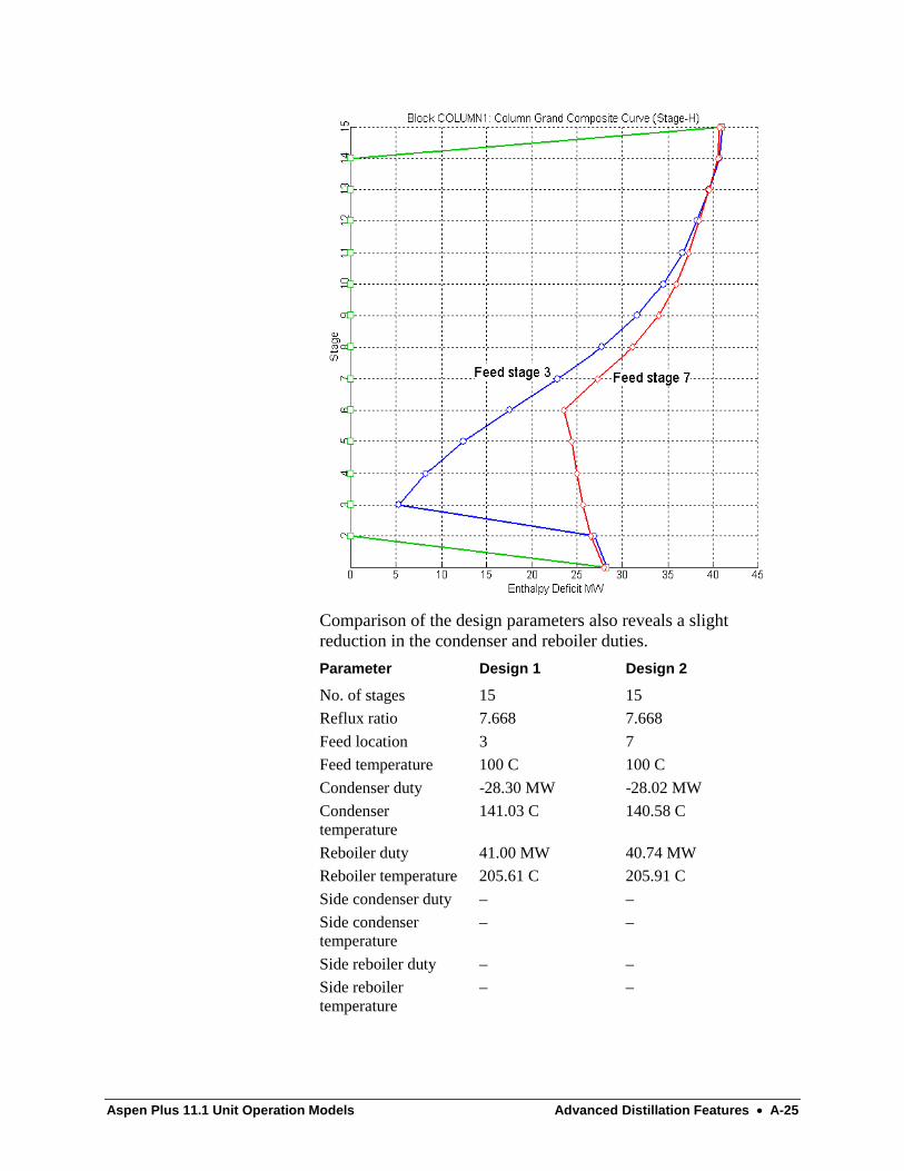
Aspen Plus 11.1 Unit Operation Models Advanced Distillation Features • A-25
Comparison of the design parameters also reveals a slightreduction in the condenser and reboiler duties.
Parameter Design 1 Design 2
No. of stages 15 15
Reflux ratio 7.668 7.668
Feed location 3 7
Feed temperature 100 C 100 C
Condenser duty -28.30 MW -28.02 MW
Condensertemperature
141.03 C 140.58 C
Reboiler duty 41.00 MW 40.74 MW
Reboiler temperature 205.61 C 205.91 C
Side condenser duty – –
Side condensertemperature
– –
Side reboiler duty – –
Side reboilertemperature
– –

A-26 • Advanced Distillation Features Aspen Plus 11.1 Unit Operation Models
The horizontal gap between the T-H CGCC pinch point and theordinate represents the scope for reduction in heat duties throughreduction in reflux ratio. As the reflux ratio is reduced (whileincreasing the number of stages to preserve the separation), theCGCC will move towards the ordinate, thus reducing both thecondenser and reboiler loads.
The T-H CGCC for Design 2 of our distillation column is shown inthe following figure. This figure also identifies the scope forreduction in condenser and reboiler duties by reducing the refluxratio.
It must be noted that, as the reflux ratio is reduced, the number ofstages required to achieve the desired separation increases. In orderto make a judicious choice for the reflux ratio, the increase in thecapital cost due to the increase in the number of stages should betraded-off against the savings in the operating costs due to reducedcondenser and reboiler loads.
For our distillation column, if we reduce the reflux ratio to 1.227(Design 3), we have to use 30 stages to preserve the separation.The T-H CGCC for Design 3 is shown in the following figure:
Reflux Ratio Modification

Aspen Plus 11.1 Unit Operation Models Advanced Distillation Features • A-27
Comparison of the design parameters for Design 2 and Design 3reveals the energy savings achieved by reducing the reflux:
Parameter Design 2 Design 3
No. of stages 15 30
Reflux ratio 7.668 1.227
Feed location 7 14
Feed temperature 100 C 100 C
Condenser duty -28.02 MW -4.48MW
Condensertemperature
140.58 C 140.58 C
Reboiler duty 40.74 MW 17.20 MW
Reboiler temperature 205.91 C 205.91 C
Side condenser duty – –
Side condensertemperature
– –
Side reboiler duty – –
Side reboilertemperature
– –

A-28 • Advanced Distillation Features Aspen Plus 11.1 Unit Operation Models
Scope for adjustment of feed quality can be identified from sharpenthalpy changes on the Stage-H or T-H CGCC.
A feed that is excessively sub-cooled will show a sharp enthalpychange on the reboiler side of the CGCC. The extent of this changedetermines the approximate feed heating duty required. Similararguments also apply for feed cooling. Changes in the heat duty offeed pre-heaters or pre-coolers will lead to similar duty changes inthe column reboiler or condeser loads, respectively.
The Stage-H CGCC for Design 3 of our distillation column isshown in the following figure. The enthalpy change on the reboilerside is noticeably sharper. Therefore, our design can benefit fromaddition of a feed pre-heater.
Feed Conditioning

Aspen Plus 11.1 Unit Operation Models Advanced Distillation Features • A-29
Design 4 adds a feed pre-heater with a duty of 2.34 MW. Thecomparison of the design parameters for Design 3 and Design 4 isshown in the following table:
Parameter Design 3 Design 4
No. of stages 30 30
Reflux ratio 1.227 1.227
Feed location 14 14
Feed temperature 100 C 123.19 C
Condenser duty -4.48 MW -4.50 MW
Condensertemperature
140.58 C 140.80 C
Reboiler duty 17.20 MW 14.87 MW
Reboiler temperature 205.91 C 205.73 C
Side condenser duty – –
Side condensertemperature
– –
Side reboiler duty – –
Side reboilertemperature
– –
Note that feed preheating not only reduces the reboiler duty butalso reduces the temperature levels at which the hot utility (for thereboiler and for the pre-heating the feed) needs to be supplied.
Feed conditioning is normally preferred to side condensing or sidereboiling, as such modifications are external to the column andpotentially at a more convenient temperature level.
The scope for side condensing or side reboiling can be identifiedfrom the area beneath or above the CGCC pinch point (areabetween the ideal and actual enthalpy profiles). If a significant areaexists, say below the pinch, a side-condenser can be placed at anappropriate temperature level. This allows heat removal from thecolumn using a cheaper cold utility. A similar converse argumentapplies to scope for placing a side reboiler.
Side Condensing orReboiling
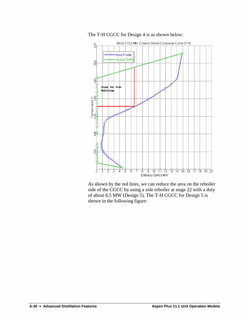
A-30 • Advanced Distillation Features Aspen Plus 11.1 Unit Operation Models
The T-H CGCC for Design 4 is as shown below:
As shown by the red lines, we can reduce the area on the reboilerside of the CGCC by using a side reboiler at stage 22 with a dutyof about 6.5 MW (Design 5). The T-H CGCC for Design 5 isshown in the following figure:
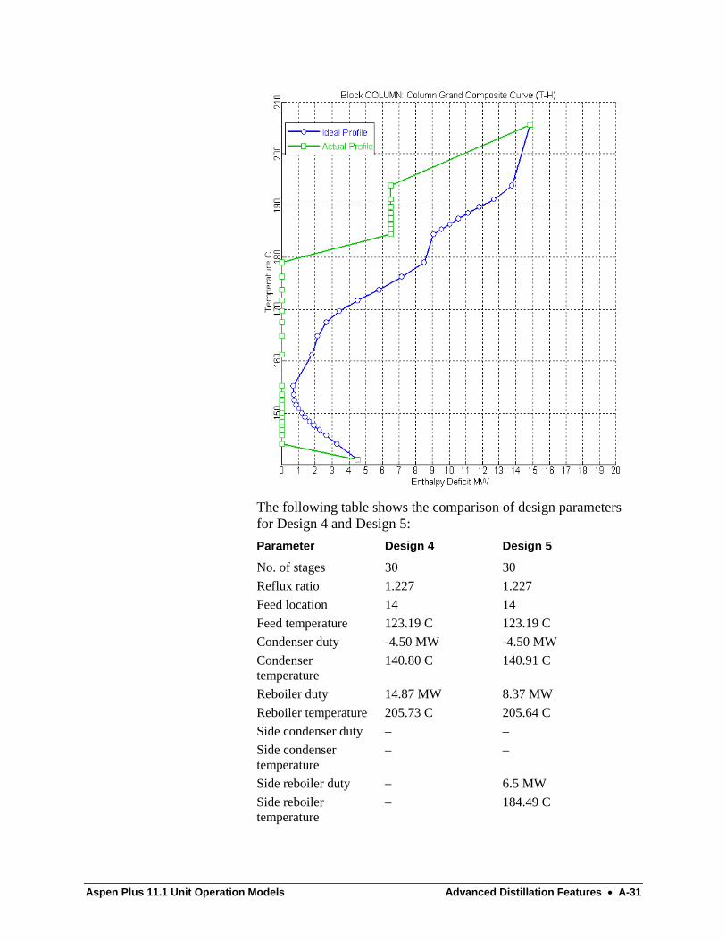
Aspen Plus 11.1 Unit Operation Models Advanced Distillation Features • A-31
The following table shows the comparison of design parametersfor Design 4 and Design 5:
Parameter Design 4 Design 5
No. of stages 30 30
Reflux ratio 1.227 1.227
Feed location 14 14
Feed temperature 123.19 C 123.19 C
Condenser duty -4.50 MW -4.50 MW
Condensertemperature
140.80 C 140.91 C
Reboiler duty 14.87 MW 8.37 MW
Reboiler temperature 205.73 C 205.64 C
Side condenser duty – –
Side condensertemperature
– –
Side reboiler duty – 6.5 MW
Side reboilertemperature
– 184.49 C

A-32 • Advanced Distillation Features Aspen Plus 11.1 Unit Operation Models
Note that, the addition of the side reboiler, not only reduces themain reboiler duty but also reduces the temperature levels at whichthe hot utility (for the main reboiler and for the side reboiler) needsto be supplied.
Exergy analysis provides a supplementary tool in identifying theabove design modification targets. For example, the exergy lossprofiles for Design 3 and Design 4 of our distillation column areshown below:
Note that the high exergy loss at the feed stage for Design 3 (due tothe sub-cooled feed) has been reduced substantially in Design 4 bypre-heating the feed.
The hydraulic analysis results show how the vapor and liquid flowsin the column compare with the minimum and maximum limits.This comparison can be used separately or in conjunction with thethermal analysis results for removing possible bottlenecks indistillation columns.
For example, let us consider that Design 2 of our distillationcolumn contains single pass sieve trays of 4.25 m diameter. The
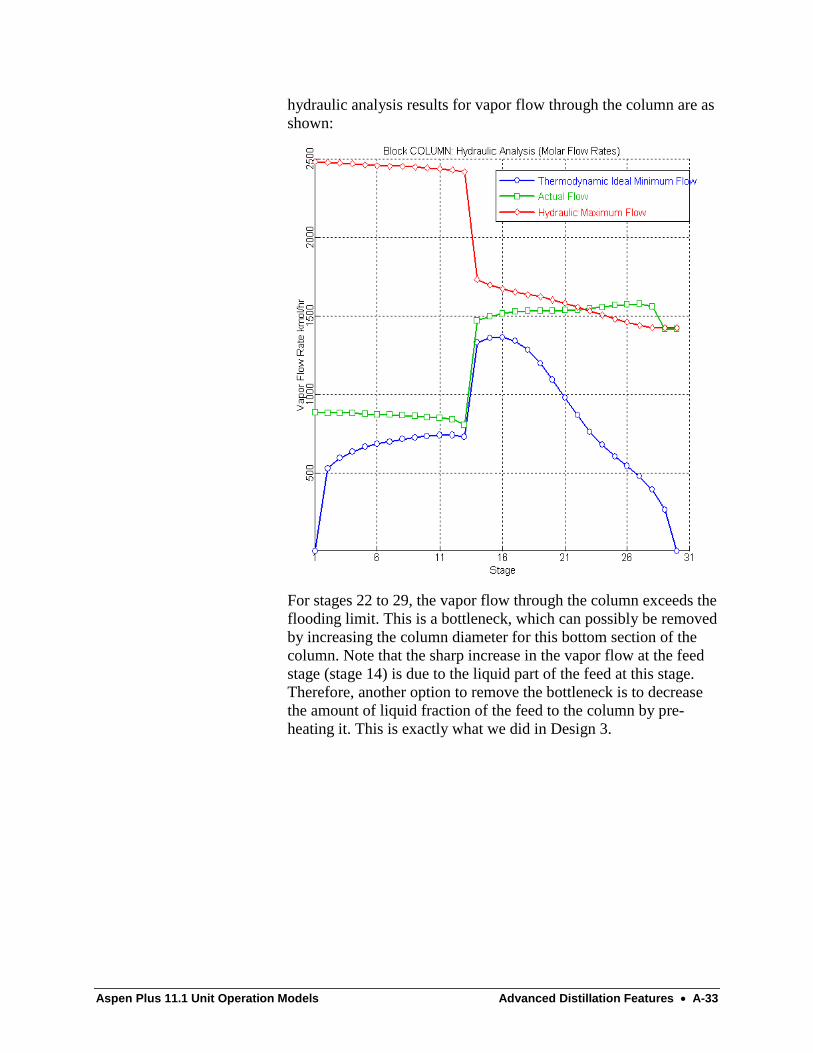
Aspen Plus 11.1 Unit Operation Models Advanced Distillation Features • A-33
hydraulic analysis results for vapor flow through the column are asshown:
For stages 22 to 29, the vapor flow through the column exceeds theflooding limit. This is a bottleneck, which can possibly be removedby increasing the column diameter for this bottom section of thecolumn. Note that the sharp increase in the vapor flow at the feedstage (stage 14) is due to the liquid part of the feed at this stage.Therefore, another option to remove the bottleneck is to decreasethe amount of liquid fraction of the feed to the column by pre-heating it. This is exactly what we did in Design 3.

A-34 • Advanced Distillation Features Aspen Plus 11.1 Unit Operation Models
The hydraulic analysis results for vapor flow through the columnfor Design 3 are as shown below:
Notice that feed pre-heating introduced in Design 2 not onlyimproved the thermal efficiency of Design 2 but also eliminatedthe vapor flow bottleneck in Design 2.
Reference
Dhole, V. R., and B. Linnhoff, “Distillation Column Targets,Computers Chem. Engng., 17, 549-560 (1993).

Aspen Plus 11.1 Unit Operation Models Index •••• 1
Index
AAbsorbers 4-57
MultiFrac: 4-28RadFrac: 4-9RateFrac 4-57, 4-58
Absorbers: 4-9, 4-28ACM
Using with Aspen Plus: 9-8ACM: 9-8ACMUser3
flowsheet connectivity: 9-8Overview: 9-8specifying: 9-8
ACMUser3: 9-8Aerotran
flash specifications: 3-26flowsheet connectivity: 3-25overview: 3-25physical properties: 3-26solids: 3-26specifying: 3-26
Aerotran: 3-25, 3-26Air separation
MultiFrac: 4-28RadFrac: 4-21
Air separation: 4-21, 4-28Air-cooled heat exchangers
Aerotran: 3-25Air-cooled heat exchangers: 3-25Algorithms
convergence: 4-20, 4-24, 4-25, 4-26, 4-39,4-40, 4-53
dynamic scenario: 10-18inside-out: 4-24, 4-40Newton: 4-20, 4-24, 4-39, 4-40nonideal: 4-20, 4-24standard: 4-24, 4-39, 4-40
sum-rates: 4-20, 4-24, 4-39, 4-40Algorithms: 4-20, 4-24, 4-25, 4-26, 4-39, 4-
40, 4-53, 10-18analysis
hydraulic A-18thermal A-18
ASME methodCompr: 6-9MCompr: 6-15
ASME method: 6-9, 6-15Aspen Custom Modeler
Using with Aspen Plus: 9-8Aspen Custom Modeler: 9-8Azeotropic distillation
RadFrac: 4-20Azeotropic distillation: 4-20
BBaffle geometry
HeatX: 3-12Baffle geometry: 3-12Baghouses
FabFl: 8-18resistance coefficients: 8-20separation efficiency: 8-21
Baghouses: 8-18, 8-20, 8-21Ballast trays
values: A-10Ballast trays: A-10Batch distillation
BatchFrac: 4-78Batch distillation: 4-78Batch fractionation
BatchFrac: 4-78Batch fractionation: 4-78Batch reactors
RBatch: 5-24Batch reactors: 5-24

2 •••• Index Aspen Plus 11.1 Unit Operation Models
BatchFraccolumns: 4-80, 4-81flowsheet connectivity: 4-80free-water calculations: 4-81physical properties: 4-82reactive distillation: 4-82specifying: 4-80three-phase calculations: 4-81working with: 4-78
BatchFrac: 4-78, 4-80, 4-81, 4-82B-JAC
Aerotran interface: 3-25Hetran interface: 3-23
B-JAC: 3-23, 3-25Bolles method
tray flooding calculations: A-8Bolles method: A-8Bond work index (BWI)
Crusher: 8-11, 8-13Bond work index (BWI): 8-11, 8-13Brake horsepower
Compr: 6-11MCompr: 6-17
Brake horsepower: 6-11, 6-17Bubble cap trays
cap diameter: A-9Bubble cap trays: A-9
CCavitation index
Valve model: 6-26Cavitation index: 6-26CCD
component attributes: 8-51flowsheet connectivity: 8-50medium temperature: 8-52mixing efficiency: 8-52overview: 8-50profiles: 8-51pseudostreams: 8-51specifying: 8-51
CCD: 8-50, 8-51, 8-52Centrifuge filters
CFuge: 8-42Centrifuge filters: 8-42CFuge
filter cake: 8-43filtrate flow rate: 8-44flowsheet connectivity: 8-42overview: 8-42pressure drop: 8-44rating: 8-43separation efficiency: 8-44sizing: 8-43specifying: 8-43
CFuge: 8-42, 8-43, 8-44Chilton-Colburn analogy
RateFrac: 4-69, 4-76Chilton-Colburn analogy: 4-69, 4-76ClChng
flowsheet connectivity: 7-6overview: 7-6specifying: 7-6stream class change: 7-6
ClChng: 7-6Coal
grinding: 8-14Coal: 8-14Column configuration
RateFrac: 4-63Column configuration: 4-63Column Targeting A-18Columns 4-57, 4-58
BatchFrac: 4-80, 4-81Distl: 4-5DSTWU: 4-3Extract: 4-84MultiFrac: 4-28operation: 4-81packings: A-11PetroFrac: 4-44physical property requirements: A-16pressure drop calculations: A-2RadFrac: 4-9, 4-13RateFrac 4-57rating: A-2SCFrac: 4-7setup: 4-80sizing: A-2
Columns: 4-3, 4-5, 4-7, 4-9, 4-13, 4-28, 4-44, 4-80, 4-81, 4-84, A-2, A-11, A-16
Component ratio

Aspen Plus 11.1 Unit Operation Models Index •••• 3
RateFrac: 4-68Component ratio: 4-68Component separators
Sep: 2-10Sep2: 2-12
Component separators: 2-10, 2-12Compr
ASME method: 6-9flowsheet connectivity: 6-9GPSA method: 6-9isentropic efficiency: 6-10mechanical efficiency: 6-11Mollier method: 6-9net work load: 6-9overview: 6-8performance curves: 6-9polytropic efficiency: 6-10specifying: 6-9steam pressure: 6-8
Compr: 6-8, 6-9, 6-10, 6-11Compressors
Compr: 6-8Heater model: 3-2MCompr: 6-13
Compressors: 3-2, 6-8, 6-13Condensers
PetroFrac: 4-48RateFrac: 4-64
Condensers: 4-48, 4-64Continuous stirred tank reactor
RCSTR: 5-16Continuous stirred tank reactor: 5-16Convergence
algorithms: 4-24, 4-39, 4-40RateFrac: 4-69
Convergence algorithmsPetroFrac: 4-53
Convergence algorithms: 4-53Convergence: 4-24, 4-39, 4-40, 4-69Coolers
Heater model: 3-2RadFrac: 4-15RateFrac: 4-67
Coolers: 3-2, 4-15, 4-67Crude units
SCFrac: 4-7
Crude units: 4-7Crusher
Bond work index (BWI): 8-11, 8-13breakage functions: 8-11flowsheet connectivity: 8-10Hardgrove grindability index (HGI): 8-11,
8-14overview: 8-10power requirement: 8-13primary crusher: 8-12reduction ratios: 8-12secondary crusher: 8-12selection functions: 8-11specifying: 8-11
Crusher: 8-10, 8-11, 8-12, 8-13, 8-14Cryogenic applications
RadFrac: 4-21Cryogenic applications: 4-21Crystallizer
crystal growth rate: 8-6crystal nucleation rate: 8-7flowsheet connectivity: 8-3magma recirculation: 8-5overview: 8-3particle size distribution (PSD): 8-8, 8-9population balance: 8-7recirculation: 8-5saturation calculation: 8-6solubility: 8-5specifying: 8-4supersaturation: 8-6
Crystallizer: 8-3, 8-4, 8-5, 8-6, 8-7, 8-8, 8-9Cyclone
design calculations: 8-23diameter calculation: 8-25dimension ratios: 8-25dimensions: 8-23, 8-27efficiency correlations: 8-24flowsheet connectivity: 8-22geometry: 8-27Leith and Licht correlation: 8-24operating ranges: 8-24overview: 8-22pressure drop: 8-24rating calculations: 8-23separation efficiency: 8-23
4 •••• Index Aspen Plus 11.1 Unit Operation Models
Shepherd and Lapple correlation: 8-24solids loading correction: 8-27specifying: 8-23vane constant: 8-26
Cyclone: 8-22, 8-23, 8-24, 8-25, 8-26, 8-27
DDarcy correlation
Pres-Relief: 10-10Darcy correlation: 10-10Decanter model
flowsheet connectivity: 2-6Gibbs free energy: 2-8KLL coefficients: 2-8liquid phases: 2-7liquid-liquid distribution coefficients: 2-8overview: 2-6phase-splitting methods: 2-8separation efficiencies: 2-8solids entrainment: 2-9specifying: 2-6, 2-7
Decanter model: 2-6, 2-7, 2-8, 2-9Decanters
CCD: 8-50Decanter model: 2-6Flash3: 2-4RadFrac: 4-15, 4-26
Decanters: 2-4, 2-6, 4-15, 4-26, 8-50Design mode
RadFrac: 4-25RateFrac: 4-68
Design mode: 4-25, 4-68Design specification convergence
MultiFrac: 4-41Design specification convergence: 4-41DIERS calculations
Pres-Relief: 10-17DIERS calculations: 10-17Distillation 4-57
batch: 4-78Distl: 4-5DSTWU: 4-3MultiFrac: 4-28PetroFrac: 4-44RadFrac: 4-9, 4-23RateFrac 4-57
SCFrac: 4-7Distillation: 4-3, 4-5, 4-7, 4-9, 4-23, 4-28, 4-
44, 4-78Distl
Edmister approach: 4-5flowsheet connectivity: 4-5overview: 4-5specifying: 4-6
Distl: 4-5, 4-6DSTWU
flowsheet connectivity: 4-4Gilliland's method: 4-3overview: 4-3reflux ratio: 4-3specifying: 4-4Underwood's method: 4-3Winn's method: 4-3
DSTWU: 4-3, 4-4Dukler correlation
Pres-Relief: 10-10Dukler correlation: 10-10Dupl 7-4
flowsheet connectivity: 7-4overview 7-4specifying: 7-5
Dupl: 7-4, 7-5Dynamic scenario algorithm
Pres-Relief: 10-18Dynamic scenario algorithm: 10-18
EEdmister approach
Distl: 4-5Edmister approach: 4-5Efficiencies
Compr: 6-10, 6-11MCompr: 6-16, 6-17RadFrac: 4-19
Efficiencies: 4-19, 6-10, 6-11, 6-16, 6-17Electrostatic precipitators
ESP: 8-32Electrostatic precipitators: 8-32Emergency relief vents (ERV)
Pres-Relief: 10-15Emergency relief vents (ERV): 10-15EO Usage Notes for User3: 9-7

Aspen Plus 11.1 Unit Operation Models Index •••• 5
Equilibrium constantsREquil: 5-10RGibbs: 5-14
Equilibrium constants: 5-10, 5-14Equilibrium reactors
REquil: 5-9RGibbs: 5-11
Equilibrium reactors: 5-9, 5-11ESP
flowsheet connectivity: 8-32gas velocity: 8-33, 8-35operating range: 8-33overview: 8-32particle separation: 8-33, 8-35power requirement: 8-35pressure drop: 8-35separation efficiency: 8-33specifying: 8-33
ESP: 8-32, 8-33, 8-35Ethylene plant primary fractionators
MultiFrac: 4-28PetroFrac: 4-44
Ethylene plant primary fractionators: 4-28,4-44
EvaporatorsFlash2: 2-2Flash3: 2-4
Evaporators: 2-2, 2-4Exchanger configuration
HeatX: 3-10Exchanger configuration: 3-10Exchanger geometry
HeatX: 3-4Exchanger geometry: 3-4Extract
flowsheet connectivity: 4-85overview: 4-84specifying: 4-85
Extract: 4-84, 4-85
FFabFl
calculation options: 8-18filtering time: 8-19flowsheet connectivity: 8-18operating ranges: 8-19
overview: 8-18resistance coefficients: 8-20separation efficiency: 8-21specifying: 8-18
FabFl: 8-18, 8-19, 8-20, 8-21Fabric filters
FabFl: 8-18Fabric filters: 8-18Fair method
tray flooding calculations: A-8Fair method: A-8Feed furnaces
PetroFrac: 4-48, 4-49Feed furnaces: 4-48, 4-49Feed stream conventions
RateFrac: 4-62Feed stream conventions: 4-62Feed streams
PetroFrac: 4-48Feed streams: 4-48Film coefficients
HeatX: 3-9, 3-14Film coefficients: 3-9, 3-14Filter model
filter cake characteristics: 8-46flowsheet connectivity: 8-45overview: 8-45pressure drop: 8-46separation efficiency: 8-47specifying: 8-45
Filter model: 8-45, 8-46, 8-47Filters
CFuge: 8-42FabFl: 8-18Filter model: 8-45
Filters: 8-18, 8-42, 8-45Flanigan correlation
Pres-Relief: 10-10Flanigan correlation: 10-10Flash tables
zone analysis: 3-21Flash tables: 3-21Flash2
electrolytes: 2-3flowsheet connectivity: 2-2overview: 2-2

6 •••• Index Aspen Plus 11.1 Unit Operation Models
solids: 2-3specifying: 2-3
Flash2: 2-2, 2-3Flash3
electrolytes: 2-5flowsheet connectivity: 2-4overview: 2-4solids: 2-5specifying: 2-5streams: 2-4
Flash3: 2-4, 2-5Flashes
Flash2: 2-2Flash3: 2-4
Flashes: 2-2, 2-4Flexitrays
values: A-10Flexitrays: A-10Float valve trays
values: A-10Float valve trays: A-10Flowsheet Connectivity for User3: 9-6Fractionators
PetroFrac: 4-44Fractionators: 4-44Free-water calculations
BatchFrac: 4-81MultiFrac: 4-43PetroFrac: 4-55RadFrac: 4-18RateFrac: 4-67
Free-water calculations: 4-18, 4-43, 4-55, 4-67, 4-81
FSplitflowsheet connectivity: 1-5overview: 1-5specifying: 1-6
FSplit: 1-5, 1-6
GGas-solid separators
Cyclone: 8-22ESP: 8-32FabFl: 8-18VScrub: 8-29
Gas-solid separators: 8-18, 8-22, 8-29, 8-32
General purpose valvesPres-Relief: 10-13
General purpose valves: 10-13Gibbs free energy
Decanter model: 2-8REquil: 5-10RGibbs: 5-11
Gibbs free energy: 2-8, 5-10, 5-11Gilliland's correlation
DSTWU: 4-3Gilliland's correlation: 4-3Glitsch Ballast method
tray flooding calculations: A-8Glitsch Ballast method: A-8GPSA method
Compr: 6-9MCompr: 6-15
GPSA method: 6-9, 6-15
HHardgrove grindability index (HGI)
Crusher: 8-11, 8-14Hardgrove grindability index (HGI): 8-11,
8-14Heat exchangers
Aerotran: 3-25computational structure: 3-21Heater model: 3-2HeatX: 3-4Hetran: 3-23log-mean temperature difference: 3-7, 3-
20MHeatX: 3-19multistream: 3-19zone analysis: 3-21
Heat exchangers: 3-2, 3-4, 3-7, 3-19, 3-20,3-21, 3-23, 3-25
Heat transfer coefficientHeatX: 3-8
Heat transfer coefficient: 3-8Heater model
electrolytes: 3-3flowsheet connectivity: 3-2overview: 3-2solids: 3-3specifying: 3-2, 3-3

Aspen Plus 11.1 Unit Operation Models Index •••• 7
Heater model: 3-2, 3-3Heaters
Heater model: 3-2MultiFrac: 4-36RadFrac: 4-15RateFrac: 4-67
Heaters: 3-2, 4-15, 4-36, 4-67Heat-interstaged columns
MultiFrac: 4-28Heat-interstaged columns: 4-28HeatX
baffle geometry: 3-12electrolytes: 3-16exchanger configuration: 3-10exchanger geometry: 3-4film coefficients: 3-9, 3-14flash specifications: 3-16flowsheet connectivity: 3-5heat transfer coefficient: 3-8log-mean temperature difference: 3-7model correlations: 3-14nozzle geometry: 3-14option sets: 3-16overview: 3-4physical properties: 3-16pressure drop calculations: 3-9, 3-14pressure drop: 3-12, 3-13, 3-14rating calculations: 3-4, 3-6, 3-7, 3-8shell-side film coefficient: 3-12solids: 3-16specifying: 3-6streams: 3-5TEMA shells: 3-10tube geometry: 3-13tube-side film coefficient: 3-13zone analysis: 3-4
HeatX: 3-4, 3-5, 3-6, 3-7, 3-8, 3-9, 3-10, 3-12, 3-13, 3-14, 3-16
HETPpackings calculations: A-11RateFrac: 4-60, 4-68
HETP: 4-60, 4-68, A-11Hetran
flash specifications: 3-24flowsheet connectivity: 3-23overview: 3-23
physical properties: 3-24solids: 3-24specifying: 3-24
Hetran: 3-23, 3-24HyCyc
dimension ratios: 8-39dimensions: 8-40feed splitting: 8-38flowsheet connectivity: 8-36geometry: 8-40operating ranges: 8-37overview: 8-36particle velocity: 8-39pressure drop correlation: 8-39rating: 8-37separation efficiency: 8-37sizing: 8-37solids separation: 8-36specifying: 8-37velocity correlation: 8-39
HyCyc: 8-36, 8-37, 8-38, 8-39, 8-40hydraulic analysis A-18Hydraulic turbines
Pump model: 6-2Hydraulic turbines: 6-2Hydrocyclones
HyCyc: 8-36Hydrocyclones: 8-36
IInside-out algorithms
MultiFrac: 4-40RadFrac: 4-24
Inside-out algorithms: 4-24, 4-40Isentropic compressors
Compr: 6-8, 6-10MCompr: 6-13
Isentropic compressors: 6-8, 6-10, 6-13Isentropic turbines
Compr: 6-8MCompr: 6-13
Isentropic turbines: 6-8, 6-13
KKnock-out drums
Decanter model: 2-6

8 •••• Index Aspen Plus 11.1 Unit Operation Models
Flash2: 2-2Flash3: 2-4
Knock-out drums: 2-2, 2-4, 2-6
LLeith and Licht correlation
Cyclone: 8-24Leith and Licht correlation: 8-24Liquid-liquid extraction
Extract: 4-84Liquid-liquid extraction: 4-84Liquid-solid separators
CFuge: 8-42Filter model: 8-45HyCyc: 8-36
Liquid-solid separators: 8-36, 8-42, 8-45LNG exchanger
MHeatX: 3-19LNG exchanger: 3-19Lockhart-Martinelli correlation
Pres-Relief: 10-10Lockhart-Martinelli correlation: 10-10Log-mean temperature difference
HeatX: 3-7MHeatX: 3-20
Log-mean temperature difference: 3-7, 3-20
MManipulators 7-4
ClChng: 7-6Dupl 7-4Mult: 7-2
Manipulators: 7-2, 7-6MCompr
ASME method: 6-15brake horsepower: 6-17flow coefficient: 6-18flowsheet connectivity: 6-14GPSA method: 6-15head coefficient: 6-18isentropic efficiency: 6-16mechanical efficiency: 6-17Mollier method: 6-15overview: 6-13parasitic pressure loss: 6-17polytropic efficiency: 6-16
specific diameter: 6-18specific speed: 6-17specifying: 6-14, 6-15
MCompr: 6-13, 6-14, 6-15, 6-16, 6-17, 6-18MHeatX
computational structure: 3-21electrolytes: 3-22flash tables: 3-21flowsheet connectivity: 3-19LNG exchanger: 3-19log-mean temperature difference: 3-20overview: 3-19pinch points estimation: 3-21solids: 3-22specifying: 3-20zone analysis: 3-19, 3-20, 3-21
MHeatX: 3-19, 3-20, 3-21, 3-22Mixer model
flowsheet connectivity: 1-2overview: 1-2specifying: 1-3
Mixer model: 1-2, 1-3Mixers
Heater model: 3-2Mixer model: 1-2
Mixers: 1-2, 3-2Model correlations
HeatX: 3-14Model correlations: 3-14Mollier method
Compr: 6-9MCompr: 6-15
Mollier method: 6-9, 6-15Mult
flowsheet connectivity: 7-2overview: 7-2specifying: 7-2
Mult: 7-2MultiFrac
algorithms: 4-40connecting streams: 4-34convergence algorithms: 4-39, 4-40design mode: 4-39design specification convergence: 4-41efficiencies: 4-38ethylene plant primary fractionator: 4-28
Aspen Plus 11.1 Unit Operation Models Index •••• 9
feed stream conventions: 4-33flow rate: 4-34, 4-36, 4-39flow ratio: 4-37flowsheet connectivity: 4-30free-water calculations: 4-43heaters: 4-36initialization methods: 4-42Murphree efficiency: 4-38Newton algorithm: 4-40overview: 4-28packings: 4-27, 4-43physical properties: 4-42property methods: 4-42rating mode: 4-39solids: 4-43specifying: 4-31, 4-32stream definitions: 4-32streams: 4-30, 4-31, 4-33, 4-34, 4-39sum-rates algorithm: 4-40trays: 4-27, 4-43vaporization efficiency: 4-38
MultiFrac: 4-27, 4-28, 4-30, 4-31, 4-32, 4-33, 4-34, 4-36, 4-37, 4-38, 4-39, 4-40,4-41, 4-42, 4-43
Multistage fractionation unitsMultiFrac: 4-28
Multistage fractionation units: 4-28Murphree efficiency
MultiFrac: 4-38PetroFrac: 4-52RadFrac: 4-19RateFrac: 4-60, 4-68
Murphree efficiency: 4-19, 4-38, 4-52, 4-60,4-68
NNapthali-Sandholm algorithm
RadFrac: 4-24Napthali-Sandholm algorithm: 4-24Nesting
RadFrac: 4-25Nesting: 4-25Newton algorithm
MultiFrac: 4-40RadFrac: 4-20, 4-24RateFrac: 4-69
Newton algorithm: 4-20, 4-24, 4-40, 4-69Nonequilibrium fractionation 4-57
RateFrac 4-57Nozzle geometry
HeatX: 3-14Nozzle geometry: 3-14
PPackings
calculations: A-11capacity calculations: A-12liquid holdup calculations: A-15MultiFrac: 4-27, 4-43PetroFrac: 4-56pressure drop calculations: A-14pressure profile: A-15RateFrac: 4-64rating: A-12sizing: A-12specifying: A-2Stichlmair correlation: A-15types: A-2, A-11, A-12
Packings: 4-27, 4-43, 4-56, 4-64, A-2, A-11,A-12, A-14, A-15
Particle separationESP: 8-33, 8-35
Particle separation: 8-33, 8-35PetroFrac
condensers: 4-48convergence algorithms: 4-53design mode: 4-54efficiencies: 4-52ethylene plant primary fractionator: 4-44feed furnace: 4-48, 4-49feed streams: 4-48flowsheet connectivity: 4-46free-water calculations: 4-55liquid runback: 4-51main column: 4-47, 4-48Murphree efficiency: 4-52overview: 4-44packings: 4-56physical properties: 4-55property methods: 4-55pumparounds: 4-51rating mode: 4-54

10 •••• Index Aspen Plus 11.1 Unit Operation Models
reboilers: 4-48side strippers: 4-47, 4-51solids: 4-55specifying: 4-48streams: 4-46trays: 4-56vaporization efficiency: 4-52
PetroFrac: 4-44, 4-46, 4-47, 4-48, 4-49, 4-51, 4-52, 4-53, 4-54, 4-55, 4-56
Petroleum refining fractionationMultiFrac: 4-28PetroFrac: 4-44
Petroleum refining fractionation: 4-28, 4-44Petroleum/petrochemical applications
RadFrac: 4-20Petroleum/petrochemical applications: 4-20Physical properties
BatchFrac: 4-82columns: A-16HeatX: 3-16
Physical properties: 3-16, 4-82, A-16Physical property methods
RateFrac: 4-67Physical property methods: 4-67Pinch points
estimating: 3-21Pinch points: 3-21Pipe model
Design-Spec convergence loop: 6-31downstream and upstream integration: 6-
30erosional velocity: 6-31fittings modeling: 6-32flash options: 6-30flowsheet connectivity: 6-29fraction factor correlations: 6-32holdup correlations: 6-32integration direction: 6-30liquid holdup correlations: 6-32methane gas systems: 6-32overview: 6-28physical property calculations: 6-30pressure drop calculations: 6-30pressure specification: 6-29specifying: 6-29stream specification: 6-30
two-phase correlations: 6-32valve modeling: 6-32
Pipe model: 6-28, 6-29, 6-30, 6-31, 6-32Pipes
Pipe model: 6-28Pipes: 6-28Piping system
Pres-Relief: 10-10Piping system: 10-10Plug flow reactors
RPlug: 5-20Plug flow reactors: 5-20Polytropic compressors
Compr: 6-8, 6-10MCompr: 6-13
Polytropic compressors: 6-8, 6-10, 6-13Pres-Relief
3% rule: 10-797% rule: 10-8Beggs and Brill correlation: 10-10calculation methods: 10-22capacity runs: 10-6code compliance: 10-6convergence methods: 10-22credit factors: 10-3Darcy correlation: 10-10data tables: 10-12, 10-13, 10-14, 10-15DIERS calculations: 10-17disengagement options: 10-17Dukler correlation: 10-10dynamic scenarios: 10-2, 10-6, 10-16, 10-
17, 10-18fire scenario: 10-3flow equations: 10-19heat exchanger shell: 10-16heat flux scenario: 10-5insulation credit factor: 10-22Lockhart-Martinelli correlation: 10-10manufacturers' tables: 10-12, 10-13, 10-
14, 10-15nozzle flow equation: 10-20overview: 10-2pipe diameters: 10-12pipe flow equation: 10-19pipe specifications: 10-10reactions: 10-9
Aspen Plus 11.1 Unit Operation Models Index •••• 11
relief system flow rating scenario: 10-5relief system: 10-9relief valve flow rating scenario: 10-5rupture disks: 10-15safety relief valves: 10-14sample solution: 10-18scenarios: 10-3sizing rules: 10-7, 10-8Slack correlation: 10-10specifying: 10-2, 10-9, 10-10spheres: 10-16steady-state scenarios: 10-6stop criteria: 10-17streams: 10-6user-specified vessel: 10-16valve cycling: 10-15valve types: 10-9, 10-13vents: 10-15vessel geometry: 10-16vessel head types: 10-16vessel jacket: 10-16X% rule: 10-7
Pres-Relief: 10-2, 10-3, 10-5, 10-6, 10-7,10-8, 10-9, 10-10, 10-12, 10-13, 10-14,10-15, 10-16, 10-17, 10-18, 10-19, 10-20, 10-22
Pressure changersCompr: 6-8MCompr: 6-13Pipe model: 6-28Pump model: 6-2Valve model: 6-19
Pressure changers: 6-2, 6-8, 6-13, 6-19, 6-28Pressure drop calculations
HeatX: 3-9, 3-14Pressure drop calculations: 3-9, 3-14Pressure drop models
HeatX: 3-12, 3-13, 3-14Pipe model: 6-28
Pressure drop models: 3-12, 3-13, 3-14, 6-28Pressure relief systems
Pres-Relief: 10-2Pressure relief systems: 10-2Pump model
flow coefficient: 6-6flowsheet connectivity: 6-3
head coefficient: 6-6net positive suction head (NPSH): 6-4overview: 6-2specific speed: 6-4specifying: 6-3suction specific speed: 6-5
Pump model: 6-2, 6-3, 6-4, 6-5, 6-6Pumparounds
RadFrac: 4-16Pumparounds: 4-16Pumps
Heater model: 3-2Pump model: 6-2
Pumps: 3-2, 6-2
RRadFrac
absorbers: 4-21air separation: 4-21algorithms: 4-20azeotropic distillation: 4-20column configuration: 4-12, 4-13convergence algorithms: 4-20, 4-24convergence methods: 4-24, 4-25, 4-26coolers: 4-15decanters: 4-15, 4-26design mode convergence: 4-25design mode: 4-22design specifications: 4-25efficiencies: 4-19feed streams: 4-12flowsheet connectivity: 4-11free-water calculations: 4-18heaters: 4-15inside-out algorithms: 4-24kettle reboilers: 4-13Murphree efficiency: 4-19Napthali-Sandholm algorithm: 4-24nested algorithm: 4-25Newton algorithm: 4-20, 4-24nonideal systems: 4-20overview: 4-9petroleum/petrochemical applications: 4-
20physical properties: 4-26property methods: 4-26
12 •••• Index Aspen Plus 11.1 Unit Operation Models
pumparounds: 4-16rating mode: 4-21reactive distillation: 4-23reboilers: 4-13salt precipitation: 4-23simultaneous convergence: 4-26solids handling: 4-26specifying: 4-11, 4-12stage numbering: 4-12streams: 4-11strippers: 4-21thermosyphon reboilers: 4-13three-phase calculations: 4-18, 4-21two-phase calculations: 4-21UA calculations: 4-15vaporizaton efficiency: 4-19
RadFrac: 4-9, 4-11, 4-12, 4-13, 4-15, 4-16,4-18, 4-19, 4-20, 4-21, 4-22, 4-23, 4-24,4-25, 4-26
Rate-based modelingRateFrac 4-57RateFrac: 4-60
Rate-based modeling: 4-60RateFrac 4-57
bubble-cap tray column: 4-74Chilton-Colburn analogy: 4-69, 4-76column configuration: 4-63column numbering: 4-62component ratio: 4-68connecting streams: 4-64convergence: 4-69coolers: 4-67correlations: 4-69, 4-71design mode: 4-68efficiencies: 4-60, 4-68equilibrium stages: 4-66feed stream conventions: 4-62flowsheet connectivity: 4-59Fortran subroutines: 4-69free-water calculations: 4-67heat transfer coefficients: 4-76heaters: 4-67HETP: 4-60, 4-68interfacial areas: 4-69, 4-71, 4-72, 4-74, 4-
75
mass transfer coefficients: 4-69, 4-71, 4-72, 4-74, 4-75
Murphree efficiency: 4-60, 4-68Newton algorithm: 4-69overview 4-57packing specifications: 4-64physical property method: 4-67rate-based modeling: 4-60rating mode: 4-67reactions: 4-66reactive distillation: 4-66segments: 4-62, 4-64, 4-68side duties: 4-67sieve tray column correlations: 4-75solution times: 4-69specifying: 4-59, 4-62, 4-64stream definitions: 4-62streams: 4-59tray column correlations: 4-74, 4-75tray column: 4-72tray specifications: 4-64utility exchangers: 4-67valve tray column: 4-72
RateFrac: 4-59, 4-60, 4-62, 4-63, 4-64, 4-66,4-67, 4-68, 4-69, 4-71, 4-72, 4-74, 4-75,4-76
Rating modeRateFrac: 4-67
Rating mode: 4-67RBatch
batch operation: 5-28cycle time: 5-27flowsheet connectivity: 5-24mass balances: 5-27overview: 5-24reactions: 5-26specifying: 5-25stop criteria: 5-27temperature controller: 5-26
RBatch: 5-24, 5-25, 5-26, 5-27, 5-28RCSTR
flowsheet connectivity: 5-16overview: 5-16phase volume: 5-17reaction kinetics: 5-17residence time: 5-18
Aspen Plus 11.1 Unit Operation Models Index •••• 13
scaling methods: 5-18solids reactions: 5-18specifying: 5-17variable scaling: 5-18
RCSTR: 5-16, 5-17, 5-18Reactions
RateFrac: 4-66Reactions: 4-66Reactive distillation
BatchFrac: 4-82RadFrac: 4-23
Reactive distillation: 4-23, 4-82Reactors
RBatch: 5-24RCSTR: 5-16REquil: 5-9RGibbs: 5-11RPlug: 5-20RStoic: 5-3RYield: 5-7
Reactors: 5-3, 5-7, 5-9, 5-11, 5-16, 5-20, 5-24
ReboilersPetroFrac: 4-48RadFrac: 4-13
Reboilers: 4-13, 4-48Relief devices
Pres-Relief: 10-9Relief devices: 10-9REquil
equilibrium constants: 5-10flowsheet connectivity: 5-9Gibbs free energy: 5-10net heat duty: 5-9overview: 5-9solids: 5-10specifying: 5-10streams: 5-9
REquil: 5-9, 5-10RGibbs
chemical equilibrium: 5-13flowsheet connectivity: 5-11overview: 5-11phase equilibrium: 5-12, 5-14reactions: 5-14restricted chemical equilibrium: 5-14
solids: 5-15specifying: 5-12
RGibbs: 5-11, 5-12, 5-13, 5-14, 5-15Rigorous distillation 4-57
MultiFrac: 4-28PetroFrac: 4-44RadFrac: 4-9RateFrac 4-57
Rigorous distillation: 4-9, 4-28, 4-44Rigorous extraction
Extract: 4-84Rigorous extraction: 4-84RPlug
coolant: 5-22flowsheet connectivity: 5-20overview: 5-20reactions: 5-23solids: 5-23specifying: 5-22
RPlug: 5-20, 5-22, 5-23RStoic
flowsheet connectivity: 5-3heat of reaction: 5-4overview: 5-3product selectivity: 5-4, 5-5specifying: 5-4stream specifications: 5-3
RStoic: 5-3, 5-4, 5-5RYield
calculation types: 5-8flowsheet connectivity: 5-7heat duty specification: 5-7overview: 5-7specifying: 5-8yield distribution: 5-8
RYield: 5-7, 5-8
SSalt precipitation
RadFrac: 4-23Salt precipitation: 4-23SCFrac
crude units: 4-7flowsheet connectivity: 4-7overview: 4-7specifying: 4-8

14 •••• Index Aspen Plus 11.1 Unit Operation Models
vacuum towers: 4-7SCFrac: 4-7, 4-8Screen
flowsheet connectivity: 8-15operating levels: 8-16overview: 8-15screen size correlation: 8-16selection function: 8-16separation efficiency: 8-17separation strength: 8-16specifying: 8-15
Screen: 8-15, 8-16, 8-17Sep
flowsheet connectivity: 2-10inlet pressure: 2-11outlet stream conditions: 2-11overview: 2-10specifying: 2-10
Sep: 2-10, 2-11Sep2
flowsheet connectivity: 2-12inlet pressure: 2-13outlet stream conditions: 2-13overview: 2-12specifying: 2-12substreams: 2-12
Sep2: 2-12, 2-13Separators
Decanter model: 2-6Flash2: 2-2Flash3: 2-4Sep: 2-10Sep2: 2-12
Separators: 2-2, 2-4, 2-6, 2-10, 2-12Shell and tube heat exchangers
Hetran: 3-23Shell and tube heat exchangers: 3-23Shell-side film coefficient
HeatX: 3-12Shell-side film coefficient: 3-12Shepherd and Lapple correlation
Cyclone: 8-24Shepherd and Lapple correlation: 8-24Shortcut distillation
Distl: 4-5DSTWU: 4-3
SCFrac: 4-7Shortcut distillation: 4-3, 4-5, 4-7Simultaneous convergence
RadFrac: 4-26Simultaneous convergence: 4-26Sizing recommendations
Pres-Relief: 10-8Sizing recommendations: 10-8Slack correlation
Pres-Relief: 10-10Slack correlation: 10-10Solids
Crystallizer: 8-3Flash2: 2-3Flash3: 2-5Heater model: 3-3MHeatX: 3-22RGibbs: 5-15
Solids crushersCrusher: 8-10
Solids crushers: 8-10Solids separators
CFuge: 8-42Crusher: 8-10Cyclone: 8-22ESP: 8-32FabFl: 8-18Filter model: 8-45HyCyc: 8-36Screen: 8-15VScrub: 8-29
Solids separators: 8-10, 8-15, 8-18, 8-22, 8-29, 8-32, 8-36, 8-42, 8-45
Solids washersCCD: 8-50SWash: 8-48
Solids washers: 8-48, 8-50Solids: 2-3, 2-5, 3-3, 3-22, 5-15, 8-3Specifying User3: 9-7Splitters
FSplit: 1-5Sep: 2-10Sep2: 2-12SSplit: 1-8
Splitters: 1-5, 1-8, 2-10, 2-12SSplit
Aspen Plus 11.1 Unit Operation Models Index •••• 15
flowsheet connectivity: 1-8overview: 1-8specifying: 1-8
SSplit: 1-8Stichlmair correlation
packings calculations: A-15Stichlmair correlation: A-15Stoichiometric reactors
RStoic: 5-3Stoichiometric reactors: 5-3Stream classes
changing: 7-6Stream classes: 7-6Stream definitions
RateFrac: 4-62Stream definitions: 4-62Stream manipulators 7-4
ClChng: 7-6Dupl 7-4Mult: 7-2
Stream manipulators: 7-2, 7-6Stream mixers
Mixer model: 1-2Stream mixers: 1-2Stream multiplication
Mult: 7-2Stream multiplication: 7-2Stream pressure changers
Pump model: 6-2Stream pressure changers: 6-2Stream splitters
FSplit: 1-5SSplit: 1-8
Stream splitters: 1-5, 1-8Streams
combining: 1-8Flash3: 2-4splitting: 2-10, 2-12
Streams: 1-8, 2-4, 2-10, 2-12Strippers 4-57
MultiFrac: 4-28PetroFrac: 4-47, 4-51RadFrac: 4-21RateFrac 4-57
Strippers: 4-21, 4-28, 4-47, 4-51Substream splitters
SSplit: 1-8Substream splitters: 1-8Sum-rates algorithm
MultiFrac: 4-40Sum-rates algorithm: 4-40SWash
bypass fraction: 8-49flowsheet connectivity: 8-48mixing efficiency: 8-49overview: 8-48specifying: 8-49
SWash: 8-48, 8-49
TTEMA shells
HeatX: 3-10TEMA shells: 3-10thermal analysis A-18Thermosyphon reboilers
RadFrac: 4-13Thermosyphon reboilers: 4-13Three-phase calculations
BatchFrac: 4-81RadFrac: 4-18
Three-phase calculations: 4-18, 4-81Trays
Bolles method: A-8bubble cap: A-9downcomer specifications: A-3Flexitrays: A-10float valve: A-10flooding calculations: A-8foaming calculations: A-10MultiFrac: 4-27, 4-43PetroFrac: 4-56pressure drop calculations: A-10pressure profile: A-15RateFrac: 4-64rating: A-3, A-7sizing: A-3, A-7specifying: A-2types: A-2
Trays: 4-27, 4-43, 4-56, 4-64, A-2, A-3, A-7, A-8, A-9, A-10, A-15
Tube geometryHeatX: 3-13
16 •••• Index Aspen Plus 11.1 Unit Operation Models
Tube geometry: 3-13Tube-side film coefficient
HeatX: 3-13Tube-side film coefficient: 3-13Turbines
Compr: 6-8MCompr: 6-13Pump model: 6-2
Turbines: 6-2, 6-8, 6-13
UUA calculations
RadFrac: 4-15UA calculations: 4-15Underwood's method
DSTWU: 4-3Underwood's method: 4-3Unit operation models
user-supplied: 9-2, 9-4, 9-8Unit operation models: 9-2, 9-4, 9-8User model
flowsheet connectivity: 9-2Fortran subroutines: 9-3overview: 9-2specifying: 9-3
User model: 9-2, 9-3User2
flowsheet connectivity: 9-4Fortran subroutines: 9-5overview: 9-4specifying: 9-5
User2: 9-4, 9-5User3
flowsheet connectivity: 9-6specifying: 9-7
User3: 9-6, 9-7
VVacuum filters
Filter model: 8-45Vacuum filters: 8-45Vacuum towers
SCFrac: 4-7Vacuum towers: 4-7Valve model
calculation types: 6-19
cavitation index: 6-26characteristic equation: 6-24choked flow: 6-26flow coefficient: 6-23flowsheet connectivity: 6-19overview: 6-19piping geometry factor: 6-24pressure drop calculation: 6-19, 6-26pressure drop ratio factor: 6-20pressure recovery factor: 6-22specifying: 6-19
Valve model: 6-19, 6-20, 6-22, 6-23, 6-24,6-26
Valvescycling: 10-15Heater model: 3-2Pipe model: 6-32safety relief: 10-14types used in Pres-Relief: 10-9, 10-13, 10-
14, 10-15Valve model: 6-19
Valves: 3-2, 6-19, 6-32, 10-9, 10-13, 10-14,10-15
Vaporization efficiencyMultiFrac: 4-38PetroFrac: 4-52RadFrac: 4-19
Vaporization efficiency: 4-19, 4-38, 4-52Vents
Pres-Relief: 10-15Vents: 10-15Venturi scrubbers
VScrub: 8-29Venturi scrubbers: 8-29VScrub
flowsheet connectivity: 8-29overview: 8-29pressure drop: 8-30rating: 8-30separation efficiency: 8-31sizing: 8-30specifying: 8-30
VScrub: 8-29, 8-30, 8-31
WWinn's method

Aspen Plus 11.1 Unit Operation Models Index •••• 17
DSTWU: 4-3Winn's method: 4-3Working with Feedbl: 7-9Working with Measurement: 7-14Working with User3: 9-6
YYield reactors
RYield: 5-7Yield reactors: 5-7
ZZone analysis
HeatX: 3-4MHeatX: 3-19, 3-20, 3-21
Zone analysis: 3-4, 3-19, 3-20, 3-21

18 •••• Index Aspen Plus 11.1 Unit Operation Models