Tutorial: Robustness and Optimization
106
Tutorial: Robustness and Optimization John Duchi UAI 2020
Transcript of Tutorial: Robustness and Optimization

Tutorial: Robustness and Optimization
John Duchi
UAI 2020

Outline
Part I: (convex) optimization
1 Convex optimization
2 Formulation and “technology”
Part II: robust optimization
1 Formulation of robust optimization problems
2 Data uncertainty and construction
Part III: distributional robustness
1 Ambiguity and confidence
2 Uniform performance and sub-population robustness
Part IV: valid predictions
1 Conformal inference
2 Robustness to the future?

Optimization
Basic optimization
minimize f0(x)
subject to fi(x) ≤ 0, i = 1, . . . ,m
I x ∈ Rd is variable (or decision variable)
I f0 : Rd → R is objective
I fi : Rd → R are constraints
solution is x? minimizing f0 subject to constraints

Applications and examples
Operations research (1940s on)
I Facility placement: choose location of facility minimize cost oftransporting materials
I Portfolio optimization: minimize risk or variance subject toexpected returns of investments
Engineering and control (1980s on)
I Control: minimize expended energy subject to moving fromone location to another (variables are control inputs)
I Device design: (e.g.) minimize power consumption subject tomanufacturing limits, timing requirements, size
Statistics and machine learning (1990s on)
I minimize prediction error or model mis-fit subject to priorinformation, sparsity, parameter limits

Convex optimization problems
minimize f0(x)
subect to fi(x) = 0, i = 1, . . . ,m
hi(x) = bi, i = 1, . . . , p
I objective f0 and inequality constraints fi are convex:
f(λx+ (1− λ)y) ≤ λf(x) + (1− λ)f(y) for 0 ≤ λ ≤ 1
I equalities hi are linear:
hi(x) = aTi x
this is a technology

Linear programs
objective and constraints are linear
minimize cTx
subject toAx b, Fx = g

Quadratic programs
objective and inequality constraints are quadratic
minimize xTAx+ bTx
subject to xTPix+ qTi x+ ri ≤ 0, i = 1, . . . ,m
Fx = g

Semidefinite programs
variables are matrices X ∈ Sn = X ∈ Rn×n | X = XT ,constraints are in semidefinite order
minimize tr(CX)
subject to tr(AiX) = bi, i = 1, . . . ,m
X 0

Example: matrix completion
I partially observed matrix M ∈ Rm×n+ of movie ratings in
locations (i, j) ∈ Ω
I user i represented by vector ui ∈ Rr, movie j by vj , andMij = uTi vj
For X = UV T , U ∈ Rm×r, V ∈ Rn×r,
minimize rank(X)
subject to XΩ = MΩ
has convex relaxation
minimizen∑i=1
σi(X) = ‖X‖∗
subject to XΩ = MΩ
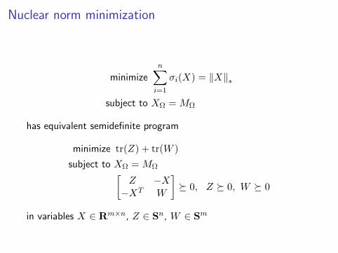
Nuclear norm minimization
minimizen∑i=1
σi(X) = ‖X‖∗
subject to XΩ = MΩ
has equivalent semidefinite program
minimize tr(Z) + tr(W )
subject to XΩ = MΩ[Z −X−XT W
] 0, Z 0, W 0
in variables X ∈ Rm×n, Z ∈ Sn, W ∈ Sm
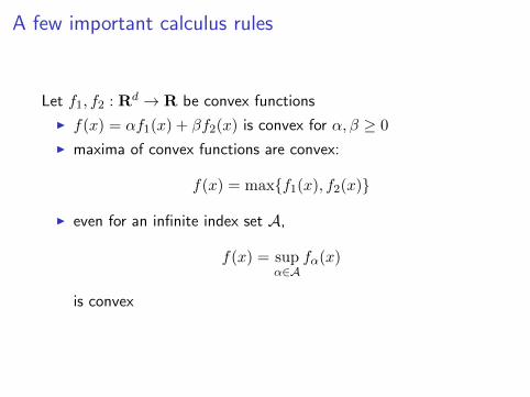
A few important calculus rules
Let f1, f2 : Rd → R be convex functions
I f(x) = αf1(x) + βf2(x) is convex for α, β ≥ 0
I maxima of convex functions are convex:
f(x) = maxf1(x), f2(x)
I even for an infinite index set A,
f(x) = supα∈A
fα(x)
is convex

A failure of linear programming
c =
100
199.9−5500−6100
A =
−.01 −.02 .5 .61 1 0 00 0 90 1000 0 40 50
100 199.9 700 800−I4
and b =
010002000800
1000000000
.
c vector of costs/profits for two drugs, constraints Ax b onproduction
I what happens if we vary percentages .01, .02 (chemicalcomposition of raw materials) by .5% and 2%, i.e..01± .00005 and .02± .0004?

Example failure for linear programming
0.00 0.05 0.10 0.15 0.20 0.250
100
200
300
400
500
600
700
800
relative change
Fre
qu
ency
Frequently lose 15–20% of profits

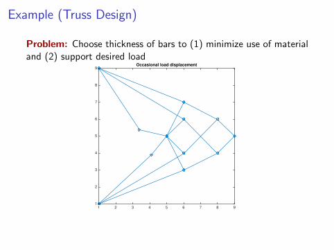
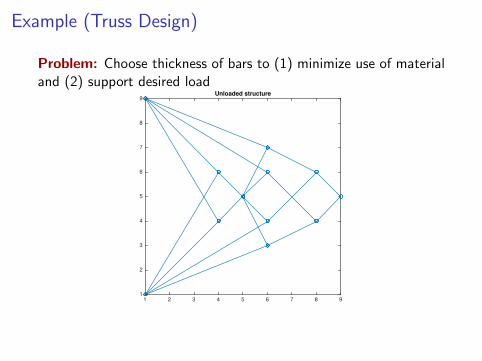
Example (Truss Design)
Problem: Choose thickness of bars to (1) minimize use of materialand (2) support desired load
1 2 3 4 5 6 7 8 9
1
2
3
4
5
6
7
8
9Unloaded structure
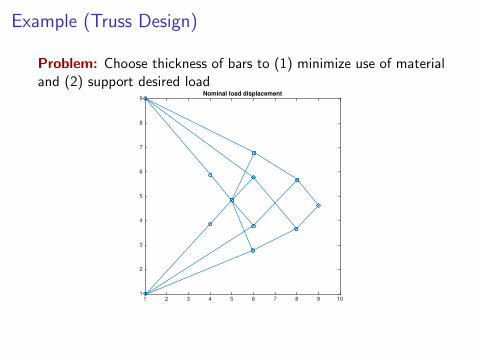
Example (Truss Design)
Problem: Choose thickness of bars to (1) minimize use of materialand (2) support desired load
1 2 3 4 5 6 7 8 9 10
1
2
3
4
5
6
7
8
9Nominal load displacement

Example (Truss Design)
Problem: Choose thickness of bars to (1) minimize use of materialand (2) support desired load
1 2 3 4 5 6 7 8 9
1
2
3
4
5
6
7
8
9Occasional load displacement

Tutorial: Robustness and Optimization
John Duchi
UAI 2020

Outline
Part I: (convex) optimization
1 Convex optimization
2 Formulation and “technology”
Part II: robust optimization
1 Formulation of robust optimization problems
2 Data uncertainty and construction
Part III: distributional robustness
1 Ambiguity and confidence
2 Uniform performance and sub-population robustness
Part IV: valid predictions
1 Conformal inference
2 Robustness to the future?

Robust optimization
objective f0 : Rn → R, uncertainty set U , fi : Rn × U → R,
fi(x, u) convex in x for all u ∈ Ugeneral form
minimize f0(x)
subject to fi(x, u) ≤ 0 for all u ∈ U , i = 1, . . . ,m.
equivalent to
minimize f0(x)
subject to supu∈U
fi(x, u) ≤ 0, i = 1, . . . ,m.
I Bertsimas, Ben-Tal, El-Ghaoui, Nemirovski (1990s–now)

Setting up robust problem
I can replace objective f0 with supu∈U f0(x, u), rewrite as
minimize t
subject to supuf0(x, u) ≤ t, sup
ufi(x, u) ≤ 0, i = 1, . . . ,m
I equality constraints make no sense: a robust equalityaT (x+ u) = b for all u ∈ U?
three questions:
I is robust formulation useful?I is robust formulation computable?I how should we choose U?

A failure of linear programming
c =
100
199.9−5500−6100
A =
−.01 −.02 .5 .61 1 0 00 0 90 1000 0 40 50
100 199.9 700 800−I4
and b =
010002000800
1000000000
.
c vector of costs/profits for two drugs, constraints Ax b onproduction
I what happens if we vary percentages .01, .02 (chemicalcomposition of raw materials) by .5% and 2%, i.e..01± .00005 and .02± .0004?

Example failure for linear programming
0.00 0.05 0.10 0.15 0.20 0.250
100
200
300
400
500
600
700
800
relative change
Fre
qu
ency
Frequently lose 15–20% of profits
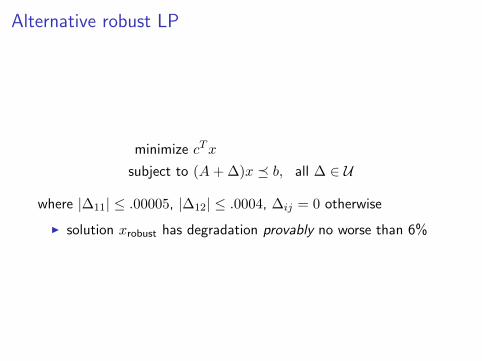
Alternative robust LP
minimize cTx
subject to (A+ ∆)x b, all ∆ ∈ U
where |∆11| ≤ .00005, |∆12| ≤ .0004, ∆ij = 0 otherwise
I solution xrobust has degradation provably no worse than 6%

Example (Truss Design)
Problem: Choose thickness of bars to (1) minimize use of materialand (2) support desired load
1 2 3 4 5 6 7 8 9
1
2
3
4
5
6
7
8
9Unloaded structure

Example (Truss Design)
Problem: Choose thickness of bars to (1) minimize use of materialand (2) support desired load
1 2 3 4 5 6 7 8 9 10
1
2
3
4
5
6
7
8
9Nominal load displacement
Example (Truss Design)
Problem: Choose thickness of bars to (1) minimize use of materialand (2) support desired load
1 2 3 4 5 6 7 8 9
1
2
3
4
5
6
7
8
9Occasional load displacement
Example (Truss Design)
Problem: Choose thickness of bars to (1) minimize use of materialand (2) support desired load
1 2 3 4 5 6 7 8 9
1
2
3
4
5
6
7
8
9Unloaded structure

Example (Truss Design)
Problem: Choose thickness of bars to (1) minimize use of materialand (2) support desired load
1 2 3 4 5 6 7 8 9 10
1
2
3
4
5
6
7
8
9Nominal load displacement

Example (Truss Design)
Problem: Choose thickness of bars to (1) minimize use of materialand (2) support desired load
1 2 3 4 5 6 7 8 9
1
2
3
4
5
6
7
8
9Occasional load displacement
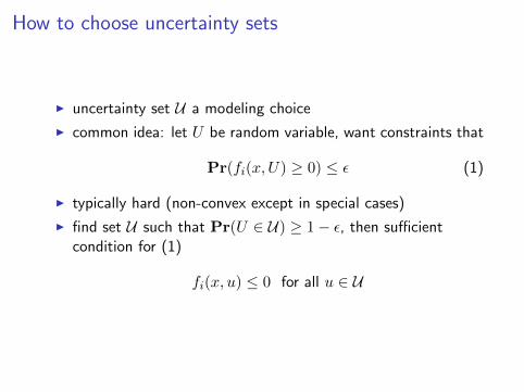
How to choose uncertainty sets
I uncertainty set U a modeling choice
I common idea: let U be random variable, want constraints that
Pr(fi(x, U) ≥ 0) ≤ ε (1)
I typically hard (non-convex except in special cases)
I find set U such that Pr(U ∈ U) ≥ 1− ε, then sufficientcondition for (1)
fi(x, u) ≤ 0 for all u ∈ U

Uncertainty set with Gaussian data
minimize cTx
subject to Pr(aTi x > bi) ≤ ε, i = 1, . . . ,m
coefficient vectors ai i.i.d. N (a,Σ) and failure probability ε
I marginally aTi x ∼ N (aTi x, xTΣx)
I for ε = .5, just LP
minimize cTx subject to aTi x ≤ bi, i = 1, . . . ,m
I what about ε = .1, .9?
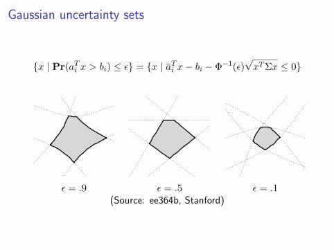
Gaussian uncertainty sets
x | Pr(aTi x > bi) ≤ ε = x | aTi x− bi − Φ−1(ε)√xTΣx ≤ 0
ε = .9 ε = .5 ε = .1(Source: ee364b, Stanford)

Robust problems are convex, so no problem?
not quite...consider quadratic constraint
‖Ax+Bu‖2 ≤ 1 for all ‖u‖∞ ≤ 1
I convex quadratic maximization in u
I solutions on extreme points u ∈ −1, 1n
I and NP-hard to maximize (even approximately [Hastad])convex quadratics over hypercube

Tractability
Important question: when is a robust LP still an LP (robust SOCPan SOCP, robust SDP an SDP)
minimize cTx
subject to (A+ U)x b for U ∈ U .
can always represent formulation constraint-wise, consider only oneinequality
(a+ u)Tx ≤ b for all u ∈ U .
I Simple example: U = u ∈ Rn | ‖u‖∞ ≤ δ, then
aTx+ δ ‖x‖1 ≤ b

When are things tractable?
Duality typically used to get tractability(but we’re not going to do that)
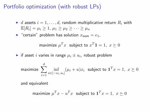
Portfolio optimization (with robust LPs)
I d assets i = 1, . . . , d, random multiplicative return Ri withE[Ri] = µi ≥ 1, µ1 ≥ µ2 ≥ · · · ≥ µn
I “certain” problem has solution xnom = e1,
maximize µTx subject to xT1 = 1, x 0
I if asset i varies in range µi ± ui, robust problem
maximized∑i=1
infu∈[−u1,ui]
(µi + u)xi subject to 1Tx = 1, x 0
and equivalent
maximize µTx− uTx subject to 1Tx = 1, x 0

Portfolio optimization (tigher control)
I Returns Ri ∈ [µi − ui, µi + ui] with ERi = µi
I guarantee return with probability 1− ε
maximizex,t t
subject to Pr
( n∑i=1
Rixi ≥ t)≥ 1− ε, xT1 = 1, x 0
I value at risk is non-convex in x, approximate it?
I approximate with high-probability bounds
I less conservative than LP (certain returns) approach
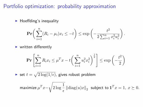
Portfolio optimization: probability approximation
I Hoeffding’s inequality
Pr
( n∑i=1
(Ri − µi)xi ≤ −t)≤ exp
(− t2
2∑n
i=1 x2iu
2i
).
I written differently
Pr
[n∑i=1
Rixi ≤ µTx− t( n∑i=1
u2ix2i
) 12
]≤ exp
(− t
2
2
)I set t =
√2 log(1/ε), gives robust problem
maximize µTx−√
2 log1
ε‖diag(u)x‖2 subject to 1Tx = 1, x 0.
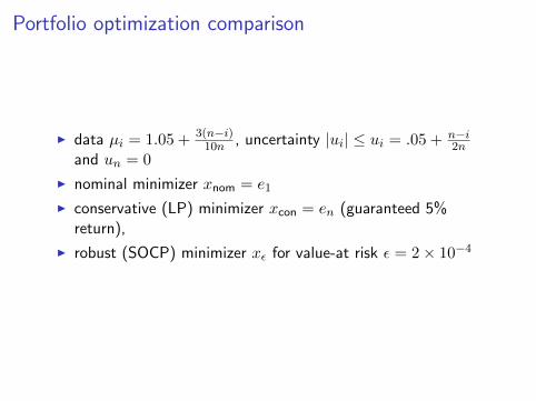
Portfolio optimization comparison
I data µi = 1.05 + 3(n−i)10n , uncertainty |ui| ≤ ui = .05 + n−i
2nand un = 0
I nominal minimizer xnom = e1
I conservative (LP) minimizer xcon = en (guaranteed 5%return),
I robust (SOCP) minimizer xε for value-at risk ε = 2× 10⁻⁴

Portfolio optimization comparison
0.6 0.8 1.0 1.2 1.4 1.6 1.8 2.00
2000
4000
6000
8000
10000
Return RTx
Fre
qu
ency
xnomxconxε
Returns chosen randomly in µi ± ui, 10,000 experiments
Tutorial: Robustness and Optimization
John Duchi
UAI 2020

Outline
Part I: (convex) optimization
1 Convex optimization
2 Formulation and “technology”
Part II: robust optimization
1 Formulation of robust optimization problems
2 Data uncertainty and construction
Part III: distributional robustness
1 Ambiguity and confidence
2 Uniform performance and sub-population robustness
Part IV: valid predictions
1 Conformal inference
2 Robustness to the future?
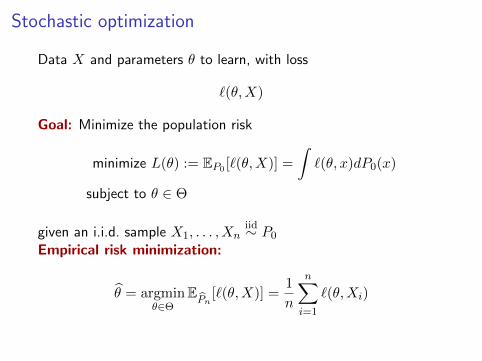
Stochastic optimization
Data X and parameters θ to learn, with loss
`(θ,X)
Goal: Minimize the population risk
minimize L(θ) := EP0 [`(θ,X)] =
∫`(θ, x)dP0(x)
subject to θ ∈ Θ
given an i.i.d. sample X1, . . . , Xniid∼ P0
Empirical risk minimization:
θ = argminθ∈Θ
EPn
[`(θ,X)] =1
n
n∑i=1
`(θ,Xi)

Curly fries and intelligence
Unlikely to be robust to even small changes in the underlying data

Revisiting uncertainty sets
minimize f0(x)
subject to fi(x, u) ≤ 0, all u ∈ U
the basic idea so far:
I assume uncertainty variable U , choose U so that
Pr(U ∈ U) ≥ 1− ε
I use this U in problem above
When do we actually know Pr(U ∈ U)?

Distributionally robust optimization
Idea: Replace distribution P0 with “uncertainty” set P of possibledistributions around P0
minimizeθ∈Θ L(θ) = EP0 [`(θ,X)]
Big question: How do we choose the set P?
(i) Hypothesis testing, covariance, and other moment constraints
(ii) Non-parametric approaches

Distributionally robust optimization
Idea: Replace distribution P0 with “uncertainty” set P of possibledistributions around P0
minimizeθ∈Θ L(θ,P) := supP∈P
EP [`(θ,X)]
Big question: How do we choose the set P?
(i) Hypothesis testing, covariance, and other moment constraints
(ii) Non-parametric approaches
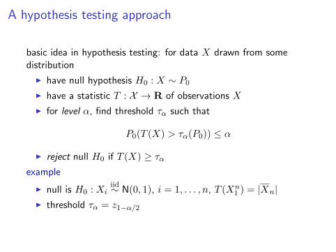
A hypothesis testing approach
basic idea in hypothesis testing: for data X drawn from somedistribution
I have null hypothesis H0 : X ∼ P0
I have a statistic T : X → R of observations X
I for level α, find threshold τα such that
P0(T (X) > τα(P0)) ≤ α
I reject null H0 if T (X) ≥ ταexample
I null is H0 : Xiiid∼ N(0, 1), i = 1, . . . , n, T (Xn
1 ) = |Xn|I threshold τα = z1−α/2

Hypothesis testing/confidence set duality
consider a collection of distributions P on space XI let T, τα(P ) be a statistic with level α for distributions P ∈ PI sample X ∼ P , observe tobs = T (X)
I confidence set
C(X) :=P ∈ P | PrP (T (X) ≤ tobs) > α
I then
Pr(P ∈ C(X)) ≥ 1− α
example
I normal familyP = N(θ, 1) | θ ∈ R
I confidence set (abusing notation) is means
C(Xn1 ) =
[Xn − z1−α/2, Xn + z1−α/2
]

Asymptotic validity
We say a test is asymptotically of level α for H0 : Xiiid∼ P if
lim supn→∞
P (T (Xn1 ) > τα(P )) ≤ α
I asymptotic confidence sets: for observations tobsn = T (Xn1 ),
C(Xn1 ) :=
P ∈ P | PrP (T (Xn
1 ) ≤ tobsn ) > α
I Then as n→∞, get
lim infn→∞
Pr(P ∈ C(Xn1 )) ≥ 1− α

A distributionally robust formulation
Steps:
1. choose valid (maybe asymptotically) confidence set C(Xn1 )
2. take uncertainty setPn := C(Xn
1 )
3. solve robust problem
minimizeθ∈Θ L(θ,Pn)
TheoremLet L?n = infθ∈Θ L(θ,Pn) and θn ∈ argminθ∈Θ L(θ,Pn). Then
lim supn→∞
Pr(L(θn) ≥ L?n) ≤ α.

Example: portfolio optimization
I random returns Ri ∈ Rd+ for d assets, periods i = 1, 2, . . .
(assumed i.i.d.), mean returns r = E[R]
I goalmaximize rT θ subject to θ 0, 1T θ = 1
I central limit theorem:
Rn =1
n
n∑i=1
Ri Σn =1
n
n∑i=1
(Ri −Rn)(Ri −Rn)T
have √nΣ−1/2
n (Rn − r)d N(0, I)
I lots of distributional facts about Z ∼ N(0, I) known
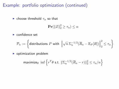
Example: portfolio optimization (continued)
I choose threshold τα so that
Pr(‖Z‖22 ≥ τα) ≤ α
I confidence set
Pn :=
distributions P with
∥∥∥√nΣ−1/2n (Rn − EP [R])
∥∥∥2
2≤ τα
I optimization problem
maximizeθ infrT θ s.t. ‖Σ−1/2
n (Rn − r)‖22 ≤ τα/n

Example behavior
Delage and Ye: Distributionally Robust Optimization Under Moment Uncertainty610 Operations Research 58(3), pp. 595–612, © 2010 INFORMS
Table 1. Comparison of short-term and long-term per-formance over six years of trading.
Singleday utility Yearly return Yearly return
(2001–2007) (2001–2004) (2004–2007)
Method Avg. 1st perc. Avg. 10th perc. Avg. 10th perc.
Our DRPO 1!000 0!983 0!944 0!846 1!102 1!025model
Popescu’s 1!000 0!975 0!700 0!334 1!047 0!936DRPOmodel
SP model 1!000 0!973 0!908 0!694 1!045 0!923
referred to as the SP model, which maximizes the averageutility over the last 30 days. We believe that the statisticsobtained over the set of 300 experiments and presented inTable 1 demonstrate how much there is to gain in terms ofaverage performance and risk reduction by considering anoptimization model that accounts for both distribution andmoment uncertainty.
First, from the analysis of the daily returns generated byeach method, one observes that they achieve comparableaverage daily utility. However, our DRPO model stands outas being more reliable. For example, the lower first per-centile of the utility distribution is 0.8% higher then thetwo competing methods. Also, this difference in reliabil-ity becomes more obvious when considering the respectivelong-term performances. Figure 1 presents the average evo-lution of wealth on a six-year period when managing aportfolio of four assets on a daily basis with any of the threemethods. In Table 1, the performances over the years 2001–2004 are presented separately from the performances overthe years 2004–2007 to measure how they are affected bydifferent levels of economic growth. The figures also peri-odically indicate the 10th and 90th percentile of the wealthdistribution over the set of 300 experiments. The statisticsof the long-term experiments demonstrate empirically that
Figure 1. Comparison of wealth evolution in 300 experiments conducted over the years 2001–2007.
2001 2002 2003 2004
0.4
0.6
0.8
1.0
1.2
1.4
1.6
Year
Wea
lth
Our DRPO modelPopescu’s DRPO modelSP model
2004 2005 2006 2007
0.50
0.75
1.00
1.25
1.50
Year
Wea
lth
Note. For each approach, the figures indicate periodically the 10th and 90th percentiles of the distribution of accumulated wealth.
our method significantly outperforms the two other ones interms of average return and risk during both the years ofeconomic growth and the years of decline. More specif-ically, our DRPO model outperformed Popescu’s DRPOmodel in terms of total return accumulated over the period2001–2007 in 79.2% of our experiments. Also, it performedon average at least 1.67 times better than any competingmodel. Note that these experiments are purely illustrativeof the strengths and weaknesses of the different models.For example, the returns measured in each experiment donot take into account transaction fees. The realized returnsare also biased due to the fact that the assets involved inour experiments were known to be major assets in theircategory in January 2007. On the other hand, the realizedreturns were also negatively biased due to the fact thatin each experiment the models were managing a portfolioof only four assets. Overall, we believe that these biasesaffected all methods equally.
Appendix. Proof of Lemma 1We first establish the primal-dual relationship betweenproblems (4) and (5). In a second step, we demonstrate thatthe conditions for strong duality to hold are met.
Step 1. One can first show, by formulating theLagrangian of problem (3), that the dual can take the fol-lowing form:
minimizer" Q" P" p" s
#$2!0 − "0"T0 % • Q + r + #!0
• P%
− 2"T0 p + $1s (22a)
subject to #TQ# − 2#T#p + Q"0% + r − h#x"#%! 0
∀# ∈! " (22b)
Q $ 0" (22c)[
P ppT s
]$ 0" (22d)
Dow
nloa
ded
from
info
rms.o
rg b
y [1
40.2
47.0
.25]
on
26 Ja
nuar
y 20
14, a
t 15:
29 .
For p
erso
nal u
se o
nly,
all
right
s res
erve
d.
(Delage and Ye, 2010)

Asymptotic risks
Challenge: often very computationally hard to use validconfidence sets (or risk is infinite)
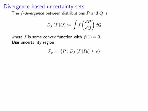
Divergence-based uncertainty setsThe f -divergence between distributions P and Q is
Df (P ||Q) :=
∫f
(dP
dQ
)dQ
where f is some convex function with f(1) = 0.

Divergence-based uncertainty setsThe f -divergence between distributions P and Q is
Df (P ||Q) :=
∫f
(dP
dQ
)dQ
where f is some convex function with f(1) = 0.Familiar examples:
I f(t) = − log t gives Df (P ||Q) = Dkl (Q||P )
I f(t) = t log t gives Df (P ||Q) = Dkl (P ||Q)
I f(t) = 12(t− 1)2 gives Dχ2 (P ||Q)
I f(t) = 12(√t− 1)2 gives d2
Hel(P,Q)
Divergence-based uncertainty setsThe f -divergence between distributions P and Q is
Df (P ||Q) :=
∫f
(dP
dQ
)dQ
where f is some convex function with f(1) = 0.Use uncertainty region
Pρ := P : Df (P ||P0) ≤ ρ

Divergence-based uncertainty setsThe f -divergence between distributions P and Q is
Df (P ||Q) :=
∫f
(dP
dQ
)dQ
where f is some convex function with f(1) = 0.Use uncertainty region
Pρ := P : Df (P ||P0) ≤ ρ
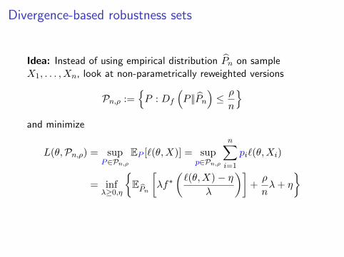
Divergence-based robustness sets
Idea: Instead of using empirical distribution Pn on sampleX1, . . . , Xn, look at non-parametrically reweighted versions
Pn,ρ :=P : Df
(P ||Pn
)≤ ρ
n
and minimize
L(θ,Pn,ρ) = supP∈Pn,ρ
EP [`(θ,X)] = supp∈Pn,ρ
n∑i=1
pi`(θ,Xi)
= infλ≥0,η
EPn
[λf∗
(`(θ,X)− η
λ
)]+ρ
nλ+ η
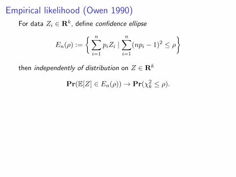
Empirical likelihood (Owen 1990)
For data Zi ∈ Rk, define confidence ellipse
En(ρ) :=
n∑i=1
piZi |n∑i=1
(npi − 1)2 ≤ ρ
then independently of distribution on Z ∈ Rk
Pr(E[Z] ∈ En(ρ))→ Pr(χ2k ≤ ρ).
−2.0 −1.5 −1.0 −0.5 0.0 0.5 1.0 1.5 2.0
−1.5
−1.0
−0.5
0.0
0.5
1.0
1.5
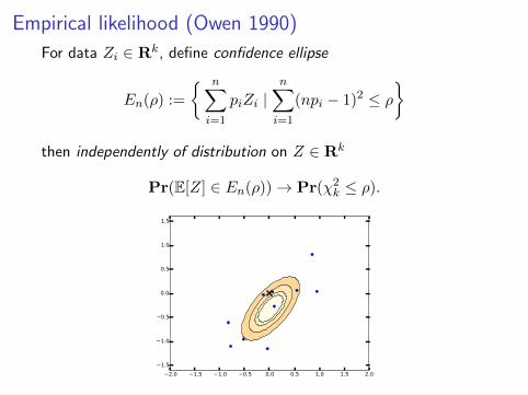
Empirical likelihood (Owen 1990)
For data Zi ∈ Rk, define confidence ellipse
En(ρ) :=
n∑i=1
piZi |n∑i=1
(npi − 1)2 ≤ ρ
then independently of distribution on Z ∈ Rk
Pr(E[Z] ∈ En(ρ))→ Pr(χ2k ≤ ρ).
−2.0 −1.5 −1.0 −0.5 0.0 0.5 1.0 1.5 2.0
−1.5
−1.0
−0.5
0.0
0.5
1.0
1.5

Empirical likelihood (Owen 1990)
For data Zi ∈ Rk, define confidence ellipse
En(ρ) :=
n∑i=1
piZi |n∑i=1
(npi − 1)2 ≤ ρ
then independently of distribution on Z ∈ Rk
Pr(E[Z] ∈ En(ρ))→ Pr(χ2k ≤ ρ).
−2.0 −1.5 −1.0 −0.5 0.0 0.5 1.0 1.5 2.0
−1.5
−1.0
−0.5
0.0
0.5
1.0
1.5

Empirical likelihood (Owen 1990)
For data Zi ∈ Rk, define confidence ellipse
En(ρ) :=
n∑i=1
piZi |n∑i=1
(npi − 1)2 ≤ ρ
then independently of distribution on Z ∈ Rk
Pr(E[Z] ∈ En(ρ))→ Pr(χ2k ≤ ρ).
−2.0 −1.5 −1.0 −0.5 0.0 0.5 1.0 1.5 2.0
−1.5
−1.0
−0.5
0.0
0.5
1.0
1.5

Empirical likelihood (Owen 1990)
For data Zi ∈ Rk, define confidence ellipse
En(ρ) :=
n∑i=1
piZi |n∑i=1
(npi − 1)2 ≤ ρ
then independently of distribution on Z ∈ Rk
Pr(E[Z] ∈ En(ρ))→ Pr(χ2k ≤ ρ).
−2.0 −1.5 −1.0 −0.5 0.0 0.5 1.0 1.5 2.0
−1.5
−1.0
−0.5
0.0
0.5
1.0
1.5
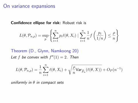
On variance expansions
Confidence ellipse for risk: Robust risk is
L(θ,Pn,ρ) = supp
n∑i=1
pi`(θ,Xi) |n∑i=1
1
nf
(pi
1/n
)≤ ρ
n
Theorem (D., Glynn, Namkoong 20)
Let f be convex with f ′′(1) = 2. Then
L(θ,Pn,ρ) =1
n
n∑i=1
`(θ,Xi) +
√ρ
nVar
Pn(`(θ,X)) +OP (n−1)
uniformly in θ in compact sets
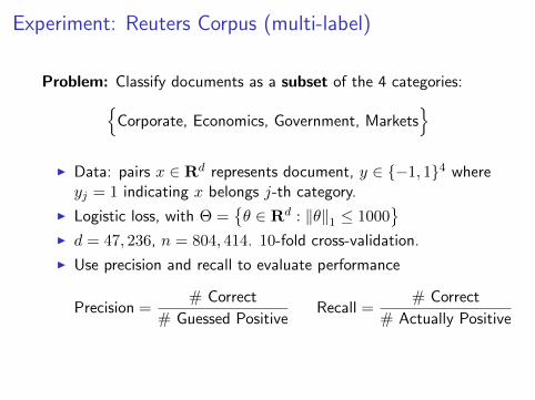
Experiment: Reuters Corpus (multi-label)
Problem: Classify documents as a subset of the 4 categories:Corporate, Economics, Government, Markets
I Data: pairs x ∈ Rd represents document, y ∈ −1, 14 whereyj = 1 indicating x belongs j-th category.
I Logistic loss, with Θ =θ ∈ Rd : ‖θ‖1 ≤ 1000
I d = 47, 236, n = 804, 414. 10-fold cross-validation.
I Use precision and recall to evaluate performance
Precision =# Correct
# Guessed PositiveRecall =
# Correct
# Actually Positive
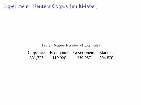
Experiment: Reuters Corpus (multi-label)
Table: Reuters Number of Examples
Corporate Economics Government Markets381,327 119,920 239,267 204,820

Experiment: Reuters Corpus (multi-label)
Figure: Recall on common category (Corporate)
ERM 103 104 105 106
ρ
0.895
0.900
0.905
0.910
0.915
0.920
0.925
0.930
0.935
Reca
ll (Corporate)
traintest
Recall
ρ
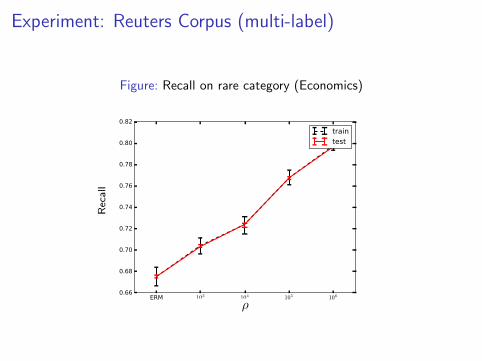
Experiment: Reuters Corpus (multi-label)
Figure: Recall on rare category (Economics)
ERM 103 104 105 106
ρ
0.66
0.68
0.70
0.72
0.74
0.76
0.78
0.80
0.82
Reca
ll (Eco
nomics)
traintest
Recall
ρ

Experiment: Reuters Corpus (multi-label)
Do well almost all the time intead of just on average
Precision Recall Precision RecallTotal Economics
50
60
70
80
90
100Test Accuracy
ERM
Robust

Moving beyond “certificates”
New challenge: doing well on sub-populations within data
I ML models increasingly used in high-stakes decisions
I Disease diagnosis, hiring decisions, driving vehiclesI Models often underperform on minority, other subpopulations
I As of 2015, only 1.9 percent of all studies of respiratorydisease included minority subjects despite African Americansmore likely to suffer respiratory ailments
I Only 2 percent of more than 10,000 cancer clinical trialsfunded by the National Cancer Institute focused on a racial orethnic minority

Approaches: group-based or pure robustness
Given groups g ∈ G with populations Pg, minimize
maxg∈G
EPg [`(θ;X)]
[Meinshausen & Buhlmann 15; Kearns et al. 19; Sagawa, Koh etal. 19–20]
I requires pre-defined groups
I may be computationally challenging (if large numbers ofpotentially intersecting groups)
alternative idea: pick worst-performing sub-population, optimizethat
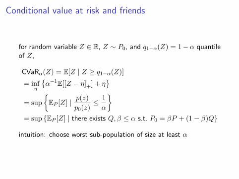
Conditional value at risk and friends
for random variable Z ∈ R, Z ∼ P0, and q1−α(Z) = 1−α quantileof Z,
CVaRα(Z) = E[Z | Z ≥ q1−α(Z)]
= infη
α−1E[[Z − η]+] + η
= sup
EP [Z] | p(z)
p0(z)≤ 1
α
= sup EP [Z] | there exists Q, β ≤ α s.t. P0 = βP + (1− β)Q
intuition: choose worst sub-population of size at least α
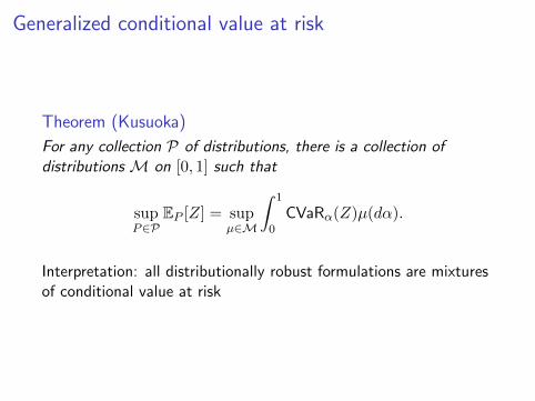
Generalized conditional value at risk
Theorem (Kusuoka)
For any collection P of distributions, there is a collection ofdistributions M on [0, 1] such that
supP∈P
EP [Z] = supµ∈M
∫ 1
0CVaRα(Z)µ(dα).
Interpretation: all distributionally robust formulations are mixturesof conditional value at risk

Robustness sets from f -divergences
Proposition (D. & Namkoong 20)
For any f of the form f(t) = tk − 1, we have
supP :Df (P ||P0)≤ρ
EP [Z] = infη
(1 + c(ρ))E
[[Z − η]k∗+
]1/k∗+ η
where k∗ = k
k−1
Consider minimizing robust losses of the form
L(θ, P : Df (P ||P0) ≤ ρ) = supP :Df (P ||P0)≤ρ
EP [`(θ;X)]

Typical results (MNIST classification experiment)
I have dataset of MNIST handwritten digits (60,000 images ofdigits 0–9)
I smaller dataset of typewritten digits
I training data is mixture of MNIST and typewritten digits

Error on MNIST handwritten digits
0.0 0.1 0.17 1.0 1.67 10.00.000
0.002
0.004
0.006
0.008
error
ρ=0ρ= . 01ρ= . 1ρ=1ρ=10ρ=50
% typewritten digits
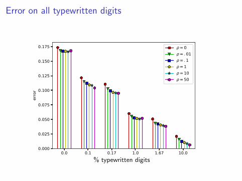
Error on all typewritten digits
0.0 0.1 0.17 1.0 1.67 10.00.000
0.025
0.050
0.075
0.100
0.125
0.150
0.175
error
ρ=0ρ= . 01ρ= . 1ρ=1ρ=10ρ=50
% typewritten digits

Error on easy typewritten digit (3)
0.0 0.1 0.17 1.0 1.67 10.00.00
0.01
0.02
0.03
0.04
0.05
0.06
0.07
error
ρ=0ρ= . 01ρ= . 1ρ=1ρ=10ρ=50
% typewritten digits

Error on hard typewritten digit (9)
0.0 0.1 0.17 1.0 1.67 10.00.00
0.05
0.10
0.15
0.20
0.25
0.30
error
ρ=0ρ= . 01ρ= . 1ρ=1ρ=10ρ=50
% typewritten digits
A few parting thoughts
I Have not talked about statistical consequences
I Still sometimes challenging to solve these at scale
I Hybrids between knowing groups and not knowing groups
I Connections with causality?

Tutorial: Robustness and Optimization
John Duchi
UAI 2020

Outline
Part I: (convex) optimization
1 Convex optimization
2 Formulation and “technology”
Part II: robust optimization
1 Formulation of robust optimization problems
2 Data uncertainty and construction
Part III: distributional robustness
1 Ambiguity and confidence
2 Uniform performance and sub-population robustness
Part IV: valid predictions
1 Conformal inference
2 Robustness to the future?

The actual robustness challenge
Robustness to future data
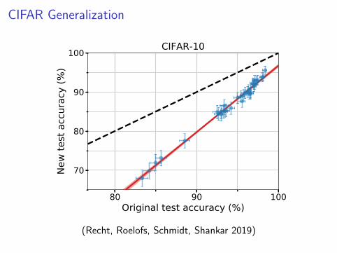
CIFAR Generalization
are an effective way to improve image classification models. Adaptivity is therefore an unlikelyexplanation for the accuracy drops.
Instead, we propose an alternative explanation based on the relative difficulty of the original andnew test sets. We demonstrate that it is possible to recover the original ImageNet accuracies almostexactly if we only include the easiest images from our candidate pool. This suggests that the accuracyscores of even the best image classifiers are still highly sensitive to minutiae of the data cleaningprocess. This brittleness puts claims about human-level performance into context [20, 31, 48]. Italso shows that current classifiers still do not generalize reliably even in the benign environment of acarefully controlled reproducibility experiment.
Figure 1 shows the main result of our experiment. Before we describe our methodology in Section 3,the next section provides relevant background. To enable future research, we release both our newtest sets and the corresponding code.1
80 90 100OriginaO test aFFuraFy (%)
70
80
90
1001
ew te
st a
FFur
aFy
(%)
CI)AR-10
Ideal reproducLbLlLty Model accuracy LLnear ILtFigure 1: Model accuracy on the original test sets vs. our new test sets. Each data point correspondsto one model in our testbed (shown with 95% Clopper-Pearson confidence intervals). The plotsreveal two main phenomena: (i) There is a significant drop in accuracy from the original to the newtest sets. (ii) The model accuracies closely follow a linear function with slope greater than 1 (1.7for CIFAR-10 and 1.1 for ImageNet). This means that every percentage point of progress on theoriginal test set translates into more than one percentage point on the new test set. The two plotsare drawn so that their aspect ratio is the same, i.e., the slopes of the lines are visually comparable.The red shaded region is a 95% confidence region for the linear fit from 100,000 bootstrap samples.
2 Potential Causes of Accuracy Drops
We adopt the standard classification setup and posit the existence of a “true” underlying datadistribution D over labeled examples (x, y). The overall goal in classification is to find a model f
1https://github.com/modestyachts/CIFAR-10.1 and https://github.com/modestyachts/ImageNetV2
2
(Recht, Roelofs, Schmidt, Shankar 2019)

ImageNet Generalization
are an effective way to improve image classification models. Adaptivity is therefore an unlikelyexplanation for the accuracy drops.
Instead, we propose an alternative explanation based on the relative difficulty of the original andnew test sets. We demonstrate that it is possible to recover the original ImageNet accuracies almostexactly if we only include the easiest images from our candidate pool. This suggests that the accuracyscores of even the best image classifiers are still highly sensitive to minutiae of the data cleaningprocess. This brittleness puts claims about human-level performance into context [20, 31, 48]. Italso shows that current classifiers still do not generalize reliably even in the benign environment of acarefully controlled reproducibility experiment.
Figure 1 shows the main result of our experiment. Before we describe our methodology in Section 3,the next section provides relevant background. To enable future research, we release both our newtest sets and the corresponding code.1
60 70 80OriginaO test accuracy (top-1, %)
40
50
60
70
801
ew te
st a
ccur
acy
(top
-1, %
) ,mage1et
Ideal reproducLbLlLty Model accuracy LLnear ILtFigure 1: Model accuracy on the original test sets vs. our new test sets. Each data point correspondsto one model in our testbed (shown with 95% Clopper-Pearson confidence intervals). The plotsreveal two main phenomena: (i) There is a significant drop in accuracy from the original to the newtest sets. (ii) The model accuracies closely follow a linear function with slope greater than 1 (1.7for CIFAR-10 and 1.1 for ImageNet). This means that every percentage point of progress on theoriginal test set translates into more than one percentage point on the new test set. The two plotsare drawn so that their aspect ratio is the same, i.e., the slopes of the lines are visually comparable.The red shaded region is a 95% confidence region for the linear fit from 100,000 bootstrap samples.
2 Potential Causes of Accuracy Drops
We adopt the standard classification setup and posit the existence of a “true” underlying datadistribution D over labeled examples (x, y). The overall goal in classification is to find a model f
1https://github.com/modestyachts/CIFAR-10.1 and https://github.com/modestyachts/ImageNetV2
2
(Recht, Roelofs, Schmidt, Shankar 2019)
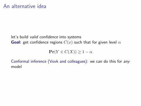
An alternative idea
let’s build valid confidence into systemsGoal: get confidence regions C(x) such that for given level α
Pr(Y ∈ C(X)) ≥ 1− α
Conformal inference (Vovk and colleagues): we can do this for anymodel

Scoring functions
I Prediction or score s(x, y)
I confidence sets of the form
C(x) = y | s(x, y) ≤ τ

Split conformal inference
Define scores Si = s(Xi, Yi), i = 1, . . . , n, and threshold
τn :=n+ 1
n(1− α)-quantile of S1, . . . , Sn
and confidence set
C(x) := y | s(x, y) ≤ τn
TheoremIf data are i.i.d., then
Pr(Yn+1 ∈ C(Xn+1)) ≥ 1− α.


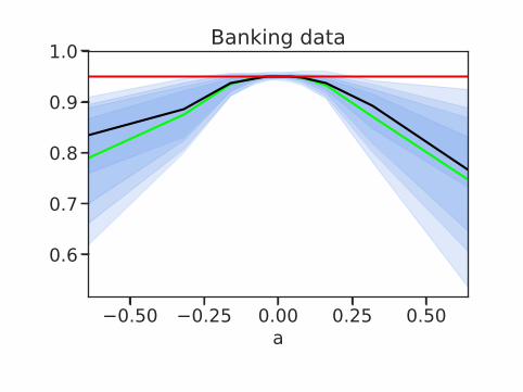
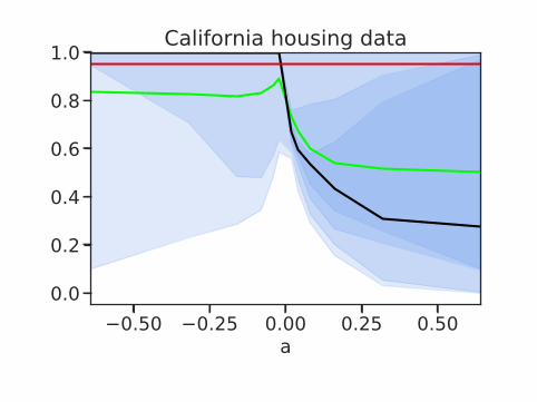
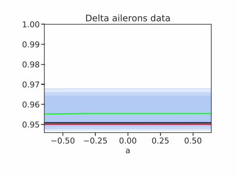
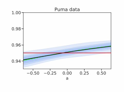
Is this enough?
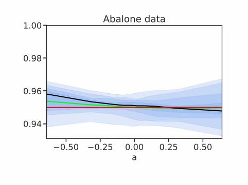
−0.50 −0.25 0.00 0.25 0.50a
0.94
0.96
0.98
1.00 Abalone data

−0.50 −0.25 0.00 0.25 0.50a
0.94
0.96
0.98
1.00 Ailerons data
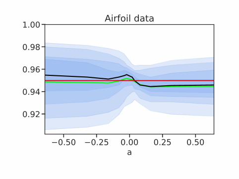
−0.50 −0.25 0.00 0.25 0.50a
0.92
0.94
0.96
0.98
1.00 Airfoil data
−0.50 −0.25 0.00 0.25 0.50a
0.6
0.7
0.8
0.9
1.0 Banking data

−0.50 −0.25 0.00 0.25 0.50a
0.4
0.6
0.8
1.0 Boston housing data
−0.50 −0.25 0.00 0.25 0.50a
0.0
0.2
0.4
0.6
0.8
1.0 California housing data
−0.50 −0.25 0.00 0.25 0.50a
0.95
0.96
0.97
0.98
0.99
1.00 Delta ailerons data

−0.50 −0.25 0.00 0.25 0.50a
0.94
0.96
0.98
1.00 Kinematics data
−0.50 −0.25 0.00 0.25 0.50a
0.94
0.96
0.98
1.00 Puma data

Distributionally robust confidence sets
Problem: Find confidence sets C(x) such that if
s(Xn+1, Yn+1) ∼ P and s(Xi, Yi)iid∼ P0 where
Df (P ||P0) ≤ ρ
thenP (Yn+1 ∈ C(Xn+1)) ≥ 1− α
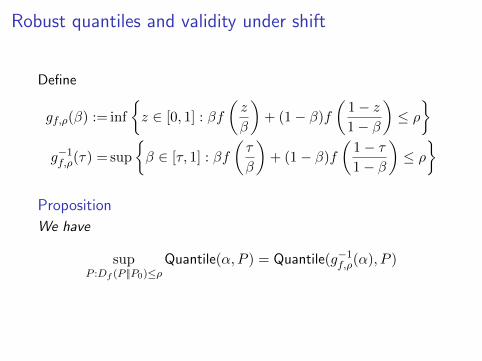
Robust quantiles and validity under shift
Define
gf,ρ(β) := inf
z ∈ [0, 1] : βf
(z
β
)+ (1− β)f
(1− z1− β
)≤ ρ
g−1f,ρ(τ) = sup
β ∈ [τ, 1] : βf
(τ
β
)+ (1− β)f
(1− τ1− β
)≤ ρ
Proposition
We have
supP :Df (P ||P0)≤ρ
Quantile(α, P ) = Quantile(g−1f,ρ(α), P )
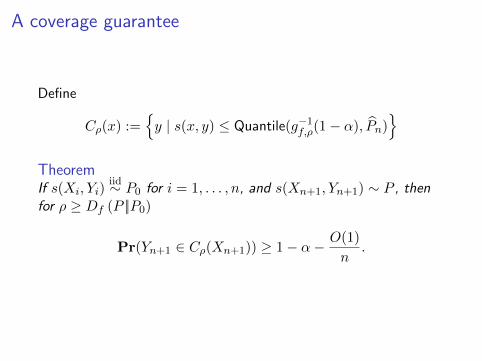
A coverage guarantee
Define
Cρ(x) :=y | s(x, y) ≤ Quantile(g−1f,ρ(1− α), Pn)
TheoremIf s(Xi, Yi)
iid∼ P0 for i = 1, . . . , n, and s(Xn+1, Yn+1) ∼ P , thenfor ρ ≥ Df (P ||P0)
Pr(Yn+1 ∈ Cρ(Xn+1)) ≥ 1− α− O(1)
n.

One experimental result
Stand
ard
Chi-squ
ared,
samplin
g
Chi-squ
ared,
regres
sion
Chi-squ
ared,
classi
ficatio
n0.80
0.85
0.90
0.95
1.00 Coverage

A few parting thoughts