
True error of a hypothesis (classi cation) Some simple...
57
Lectures 23-24: Introduction to learning theory • True error of a hypothesis (classification) • Some simple bounds on error and sample size • Introduction to VC-dimension COMP-652 and ECSE-608, Lectures 23-24, April 2017 1
Transcript of True error of a hypothesis (classi cation) Some simple...

Lectures 23-24: Introduction to learning theory
• True error of a hypothesis (classification)
• Some simple bounds on error and sample size
• Introduction to VC-dimension
COMP-652 and ECSE-608, Lectures 23-24, April 2017 1

Binary classification: The golden goal
Given:
• The set of all possible instances X
• A target function (or concept) f : X → {0, 1}• A set of hypotheses H
• A set of training examples D (containing positive and negative examplesof the target function)
〈x1, f(x1)〉, . . . 〈xm, f(xm)〉
Determine:
A hypothesis h ∈ H such that h(x) = f(x) for all x ∈ X.
COMP-652 and ECSE-608, Lectures 23-24, April 2017 2

Approximate Concept Learning
• Requiring a learner to acquire the right concept is too strict
• Instead, we will allow the learner to produce a good approximation tothe actual concept
• For any instance space, there is a non-uniform likelihood of seeingdifferent instances
• We assume that there is a fixed probability distribution D on the spaceof instances X• The learner is trained and tested on examples whose inputs are drawn
independently and randomly (iid) according to D.
COMP-652 and ECSE-608, Lectures 23-24, April 2017 3

Generalization Error and Empirical Risk
• Given a hypothesis h ∈ H, a target concept f , and an underlyingdistribution D, the generalization error or risk of h is defined by
R(h) = Ex∼D
[`(h(x), f(x))]
where ` is an error function. This measures the true error of thehypothesis.
• Given training data S = {(xi, f(xi)}mi=1, the empirical risk of h is definedby
R̂(h) =1
m
m∑i=1
`(h(xi), f(xi)).
This is the average error over the sample S, it measures the trainingerror of the hypothesis.
COMP-652 and ECSE-608, Lectures 23-24, April 2017 4

Binary Classification: 0− 1 loss
• For binary classification, a natural error measure is the 0− 1 loss, whichcounts mismatches between h(x) and f(x):
`(h(x), f(x)) = I(h(x) 6= f(x)) =
{1 if h(x) 6= f(x)0 otherwise
where I is the indicator function.
• In this case, the generalization error and empirical risk are given by
R(h) = Ex∼D
[I(h(x) 6= f(x))] = Px∼D
[h(x) 6= f(x)]
R̂(h) =1
m
m∑i=1
I(h(x) 6= f(x)).
COMP-652 and ECSE-608, Lectures 23-24, April 2017 5

The Two Notions of Error for Binary Classification
• The training error of hypothesis h with respect to target concept festimates how often h(x) 6= f(x) over the training instances
• The true error of hypothesis h with respect to target concept f estimateshow often h(x) 6= f(x) over future, unseen instances (but drawnaccording to D)
• Questions:
– Can we bound the true error of a hypothesis given its training error?i.e. can we bound the generalization error by the empirical risk?
↪→ Generalization bounds– Can we find an hypothesis with small true error after observing a
reasonable number of training points?↪→ PAC learnability
– How many examples are needed for a good approximation?↪→ Sample complexity
COMP-652 and ECSE-608, Lectures 23-24, April 2017 6

True Error of a Hypothesis
+
+-
-
f h
Instance space X
-
Where fand h disagree
COMP-652 and ECSE-608, Lectures 23-24, April 2017 7

True Error Definition
• The set of instances on which the target concept and the hypothesisdisagree is denoted: E = {x|h(x) 6= f(x)}• Using the definitions from before, the true error of h with respect to f
is: ∑x∈E
Px∼D
[x]
This is the probability of making an error on an instance randomly drawnfrom (X ,Y) according to D
• Let ε ∈ (0, 1) be an error tolerance parameter. We say that h is a goodapproximation of f (to within ε) if and only if the true error of h is lessthan ε.
COMP-652 and ECSE-608, Lectures 23-24, April 2017 8

Example: Rote Learner
• Let X = {0, 1}n. Let P be the uniform distribution over X .
• Let the concept f be generated by randomly assigning a label to everyinstance in X.
• We assume that there is no output noise, so every instance x we get islabelled with the true f(x)
• Let S ⊆ X be a set of training instances.
The hypothesis h is generated by memorizing S and giving a randomanswer otherwise.
• What is the empirical error of h?
• What is the true error of h?
COMP-652 and ECSE-608, Lectures 23-24, April 2017 9

Example: Empirical and True Error
• Since we assumed that examples are labelled correctly and memorized,the empirical error is 0• For the true error, suppose we saw m distinct examples during training,
out of the total set of 2n possible examples• For the examples we saw, we will make no error• For the (2n −m) examples we did not see, we will make an error with
probability 1/2• Hence, the true error is:
R(h) = P[h(x) 6= f(x)] =2n −m
2n1
2=(
1− m
2n
) 1
2
• Note that the true error also goes to 0 as m approaches the number ofexamples, 2n
• The difference of the true and empirical error also goes to 0 as mincreases
COMP-652 and ECSE-608, Lectures 23-24, April 2017 10
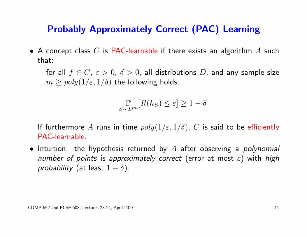
Probably Approximately Correct (PAC) Learning
• A concept class C is PAC-learnable if there exists an algorithm A suchthat:
for all f ∈ C, ε > 0, δ > 0, all distributions D, and any sample sizem ≥ poly(1/ε, 1/δ) the following holds:
PS∼Dm
[R(hS) ≤ ε] ≥ 1− δ
If furthermore A runs in time poly(1/ε, 1/δ), C is said to be efficientlyPAC-learnable.
• Intuition: the hypothesis returned by A after observing a polynomialnumber of points is approximately correct (error at most ε) with highprobability (at least 1− δ).
COMP-652 and ECSE-608, Lectures 23-24, April 2017 11

PAC learning (cont’d)
• Remarks:
– The concept class is known to the algorithm.– Distribution free model: no assumption on D.– Both training and test examples are drawn from D.
• Examples:
– Axis aligned rectangle are PAC learnable1.– Conjunctions of boolean literals are PAC learnable but the class of
disjunctions of two conjunctions is not.– Linear thresholds (e.g. perceptron) are PAC learnable but the classes
of conjunctions/disjunctions of two linear thresholds is not, nor is theclass of multilayer perceptrons.
1see [Mohri et al., Fundations of Machine Learning ] section 2.1.
COMP-652 and ECSE-608, Lectures 23-24, April 2017 12

Empirical risk minimization
• Suppose we are given a hypothesis class H• We have a magical learning machine that can sift through H and output
the hypothesis with the smallest empirical error, hemp
• This is process is called empirical risk minimization
• Is this a good idea?
• What can we say about the error of the other hypotheses in h?
COMP-652 and ECSE-608, Lectures 23-24, April 2017 13

First tool: The union bound
• Let E1 . . . Ek be k different events (not necessarily independent). Then:
P(E1 ∪ · · · ∪ Ek) ≤ P(E1) + · · ·+ P(Ek)
• Note that this is usually loose, as events may be correlated
COMP-652 and ECSE-608, Lectures 23-24, April 2017 14

Second tool: Hoeffding bound
• Hoeffding inequality. Let Z1 . . . Zm be m independent identicallydistributed (iid) random variables taking their values in [a, b]. Thenfor any ε > 0
P
[1
m
m∑i=1
Zi − E[Z] > ε
]≤ exp
(−2mε2
(b− a)2
)
COMP-652 and ECSE-608, Lectures 23-24, April 2017 15

Second tool: Hoeffding bound
• Let Z1 . . . Zm be m independent identically distributed (iid) binaryvariables, drawn from a Bernoulli (binomial) distribution:
P(Zi = 1) = φ and P(Zi = 0) = 1− φ
• Let φ̂ be the mean of these variables: φ̂ = 1m
∑mi=1Zi
• Let ε be a fixed error tolerance parameter. Then:
P(|φ− φ̂| > ε) ≤ 2e−2ε2m
• In other words, if you have lots of examples, the empirical mean is agood estimator of the true probability.
• Note: other similar concentration inequalities can be used (e.g. Chernoff,Bernstein, etc.)
COMP-652 and ECSE-608, Lectures 23-24, April 2017 16
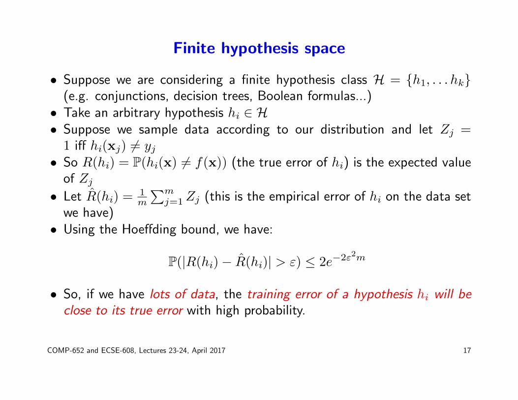
Finite hypothesis space
• Suppose we are considering a finite hypothesis class H = {h1, . . . hk}(e.g. conjunctions, decision trees, Boolean formulas...)• Take an arbitrary hypothesis hi ∈ H• Suppose we sample data according to our distribution and let Zj =
1 iff hi(xj) 6= yj• So R(hi) = P(hi(x) 6= f(x)) (the true error of hi) is the expected value
of Zj• Let R̂(hi) = 1
m
∑mj=1Zj (this is the empirical error of hi on the data set
we have)• Using the Hoeffding bound, we have:
P(|R(hi)− R̂(hi)| > ε) ≤ 2e−2ε2m
• So, if we have lots of data, the training error of a hypothesis hi will beclose to its true error with high probability.
COMP-652 and ECSE-608, Lectures 23-24, April 2017 17
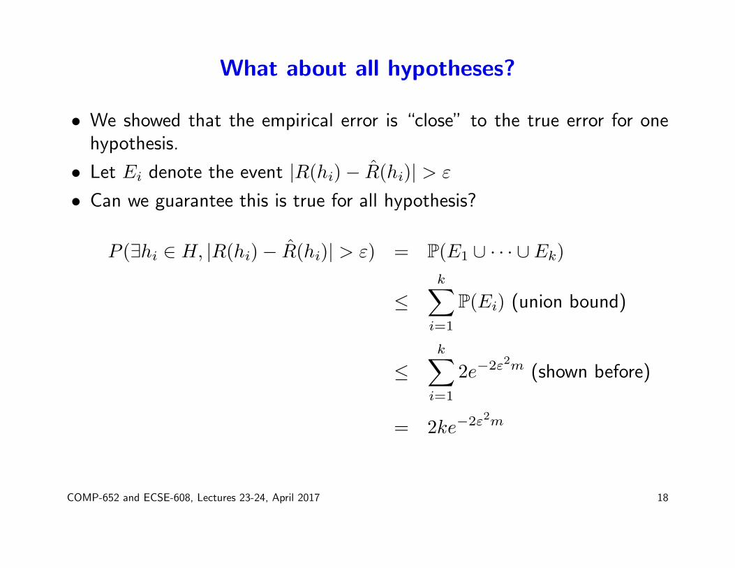
What about all hypotheses?
• We showed that the empirical error is “close” to the true error for onehypothesis.
• Let Ei denote the event |R(hi)− R̂(hi)| > ε
• Can we guarantee this is true for all hypothesis?
P (∃hi ∈ H, |R(hi)− R̂(hi)| > ε) = P(E1 ∪ · · · ∪ Ek)
≤k∑i=1
P(Ei) (union bound)
≤k∑i=1
2e−2ε2m (shown before)
= 2ke−2ε2m
COMP-652 and ECSE-608, Lectures 23-24, April 2017 18

A uniform convergence bound
• We showed that:
P(∃hi ∈ H, |R(hi)− R̂(hi)| > ε) ≤ 2ke−2ε2m
• So we have:
1− P(∃hi ∈ H, |R(hi)− R̂(hi)| > ε) ≥ 1− 2ke−2ε2m
or, in other words:
P(∀hi ∈ H, |R(hi)− R̂(hi)| < ε) ≥ 1− 2ke−2ε2m
• This is called a uniform convergence result because the bound holds forall hypotheses
• What is this good for?
COMP-652 and ECSE-608, Lectures 23-24, April 2017 19

Sample complexity
• Suppose we want to guarantee that with probability at least 1 − δ, thesample (training) error is within ε of the true error:
P (∀hi ∈ H, |R(hi)− R̂(hi)| < ε) ≥ 1− δ
• From the previous result, it would be sufficient to have: 1− 2ke−2ε2m ≥
1− δ• We get δ ≥ 2ke−2ε
2m
• Solving for m, we get that the number of samples should be:
m ≥ 1
2ε2log
2k
δ=
1
2ε2log
2|H|δ
• So the number of samples needed is logarithmic in the size of thehypothesis space and depends polynomially on 1/ε and 1/δ
COMP-652 and ECSE-608, Lectures 23-24, April 2017 20

Example: Conjunctions of Boolean Literals
• Let H be the space of all pure conjunctive formulas over n Booleanattributes.
• Then |H| = 3n, because for each of the n attributes, we can include itin the formula, include its negation, or not include it at all.
• From the previous result, we get:
m ≥ 1
2ε2log
2|H|δ
=n
2ε2log
6
δ
• This is linear in n!
• Hence, conjunctions are “easy to learn”
COMP-652 and ECSE-608, Lectures 23-24, April 2017 21

Example: Arbitrary Boolean functions
• Let H be the space of all Boolean formulae over n Boolean attributes.
• Every Boolean formula can be written in canonical form as a disjunctionof conjunctions
• We have seen that there are 3n possible conjunctions over n Booleanvariables, and for each of them, we can choose to include it or not in thedisjunction, so |H| = 23
n
• From the previous result, we get:
m ≥ 1
2ε2log
2|H|δ
=3n
2ε2log
2
δ
• This is exponential in n!
• Hence, arbitrary Boolean functions are “hard to learn”
• A similar argument can be applied to show that even restricted classesof Boolean functions, like parity and XOR, are hard to learn
COMP-652 and ECSE-608, Lectures 23-24, April 2017 22

Bounding the True Error by the Empirical Error
• Our inequality revisited:
P(∀hi ∈ H, |R(hi)− R̂(hi)| < ε) ≥ 1− 2|H|e−2ε2m ≥ 1− δ
• Suppose we hold m and δ fixed, and we solve for ε. Then we get:
|R(hi)− R̂(hi)| ≤√
1
2mlog
2|H|δ
inside the probability term.
• We are now ready to see how good empirical risk minimization is
COMP-652 and ECSE-608, Lectures 23-24, April 2017 23

Analyzing Empirical Risk Minimization
Let h∗ be the best hypothesis in our class (in terms of true error). Based onour uniform convergence assumption, we can bound the true error of hempas follows:
R(hemp) ≤ R̂(hemp) + ε
≤ R̂(h∗) + ε (because hemp has better training error
than any other hypothesis)
≤ R(h∗) + 2ε (by using the result on h∗)
≤ R(h∗) + 2
√1
2mlog
2|H|δ
(from previous slide)
This bounds how much worse hemp is, wrt the best hypothesis we can hopefor!
COMP-652 and ECSE-608, Lectures 23-24, April 2017 24

Types of error
• We showed that, given m examples, with probability at least 1− δ,
R(hemp) ≤(
minh∈H
R(h)
)+ 2
√1
2mlog
2|H|δ
• The first term is a characteristic of the hypothesis class H, also calledapproximation error
• For a hypothesis class which is consistent (can represent the targetfunction exactly) this term would be 0
• The second term decreases as the number of examples increases, butincreases with the size of the hypothesis space
• This is called estimation error and is similar in flavour to variance
• Large approximation errors lead to “under fitting”, large estimation errorslead to overfitting
COMP-652 and ECSE-608, Lectures 23-24, April 2017 25

Controlling the complexity of learning
R(hemp) ≤(
minh∈H
R(h)
)+ 2
√1
2mlog
2|H|δ
• Suppose now that we are considering two hypothesis classes H ⊆ H′• The approximation error would be smaller for H′ (we have a larger
hypothesis class) but the second term would be larger (we need moreexamples to find a good hypothesis in the larger set)
• We could try to optimize this bound directly, by measuring the trainingerror and adding to it the rightmost term (which is a penalty for the sizeof the hypothesis space)
• We would then pick the hypothesis that is best in terms of this sum!
• This approach is called structural risk minimization, and can be usedinstead of cross-validation or other types of regularization
• Note, though, that if H is infinite, this result is not very useful...
COMP-652 and ECSE-608, Lectures 23-24, April 2017 26

Example: Learning an interval on the real line
• “Treatment plant is ok iff Temperature ≤ a” for some unknown a ∈[0, 100]
• Consider the hypothesis set:
H = {[0, a]|a ∈ [0, 100]}
• Simple learning algorithm: Observe m samples, and return [0, b], whereb is the largest positive example seen
• How many examples do we need to find a good approximation of thetrue hypothesis?
• Our previous result is useless, since the hypothesis class is infinite.
COMP-652 and ECSE-608, Lectures 23-24, April 2017 27

Sample complexity of learning an interval
• Let a correspond to the true concept and let c < a be a real value s.t.[c, a] has probability ε.
• If we see an example in [c, a], then our algorithm succeeds in having trueerror smaller than ε (because our hypothesis would be less than ε awayform the true target function)
• What is the probability of seeing m iid examples outside of [c, a]?
P(failure) = (1− ε)m
• If we wantP(failure) < δ =⇒ (1− ε)m < δ
COMP-652 and ECSE-608, Lectures 23-24, April 2017 28

Example continued
• Fact:(1− ε)m ≤ e−εm (you can check that this is true)
• Hence, it is sufficient to have
(1− ε)m ≤ e−εm < δ
• Using this fact, we get:
m ≥ 1
εlog
1
δ
• You can check empirically that this is a fairly tight bound.
COMP-652 and ECSE-608, Lectures 23-24, April 2017 29

Why do we need so few samples?
• Our hypothesis space is simple - there is only one parameter to estimate!
• In other words, there is one “degree of freedom”
• As a result, every data sample gives information about LOTS ofhypotheses! (in fact, about an infinite number of them)
• What if there are more “degrees of freedom”?
COMP-652 and ECSE-608, Lectures 23-24, April 2017 30

Example: Learning two-sided intervals
• Suppose the target concept is positive (i.e. has value 1) inside someunknown interval [a, b] and negative outside of it
• The hypothesis class consists of all closed intervals (so the target can berepresented exactly.
• Given a data set D, a “conservative” hypothesis is to guess the interval:[min(x,1)∈D x,max(x,1)∈D x]
• We can make errors on either side of the interval, if we get no examplewithin ε of the true values a and b respectively.
• The probability of an example outside of an ε-size interval is 1− ε• The probability of m examples outside of it is (1− ε)m
• The probability this happens on either side is ≤ 2(1− ε)m ≤ 2e−εm, andwe want this to be < δ
COMP-652 and ECSE-608, Lectures 23-24, April 2017 31

Example (continued)
• If we extract the number of samples we get:
m ≥ 1
εln
2
δ
This is just like the bound for 1-sided intervals, but with a 2 instead ofa 1!
• Compare this with the bound in the finite case:
m ≥ 1
2ε2log
2|H|δ
• But for us, |H| =∞!
• We need a way to characterize the “complexity” of infinite-dimensionalclasses of hypotheses
COMP-652 and ECSE-608, Lectures 23-24, April 2017 32

Infinite hypothesis class
• For any set of points C = {x1, · · · , cm} ⊂ X we define the restriction ofH to C by
HC = {(h(x1), h(x2), · · · , h(xm)) : h ∈ H}.
• We showed that, given m examples, for any h ∈ H with probability atleast 1− δ,
R(h) ≤ R̂(h) +
√1
2mlog
2|H|δ
• Even if H is infinite, it is its effective size that matters: since |HC| ≤ 2m
when C has size m we can actually get
R(h) ≤ R̂(h) +
√1
2mlog
2m+1
δ
COMP-652 and ECSE-608, Lectures 23-24, April 2017 33

• But this is too loose: the second term doesn’t converge to 0...
COMP-652 and ECSE-608, Lectures 23-24, April 2017 34

VC dimension
• H ⊂ {0, 1}X is a set of hypothesis.
• For any set of points C = {x1, · · · , cm} ⊂ X we define the restriction ofH to C by
HC = {(h(x1), h(x2), · · · , h(xm)) : h ∈ H}.
• We say that H shatters C if |HC| = 2|C|.
→ If someone can explain everything, his explanations are worthless
• The VC dimension of H is the maximal size of a set C ⊂ X that can beshattered by H.
COMP-652 and ECSE-608, Lectures 23-24, April 2017 35
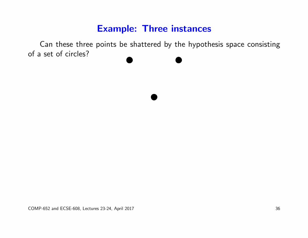
Example: Three instances
Can these three points be shattered by the hypothesis space consistingof a set of circles?
COMP-652 and ECSE-608, Lectures 23-24, April 2017 36

Example: Three instances dichotomy
Can these three points be shattered by the hypothesis space consistingof a set of circles? + +
+
COMP-652 and ECSE-608, Lectures 23-24, April 2017 37

Example: Three instances
Can these three points be shattered by the hypothesis space consistingof a set of circles?
+ +
+
COMP-652 and ECSE-608, Lectures 23-24, April 2017 38

Example: Three instances dichotomy
Can these three points be shattered by the hypothesis space consistingof a set of circles? + !
+
COMP-652 and ECSE-608, Lectures 23-24, April 2017 39

Example: Three instances
Can these three points be shattered by the hypothesis space consistingof a set of circles?
+ !
+
COMP-652 and ECSE-608, Lectures 23-24, April 2017 40

Example: Three instances dichotomy
Can three points be shattered by the hypothesis space consisting of aset of circles?
+
COMP-652 and ECSE-608, Lectures 23-24, April 2017 41

Example: Three instances
Can three points be shattered by the hypothesis space consisting of aset of circles?
+
COMP-652 and ECSE-608, Lectures 23-24, April 2017 42

Example: Three instances dichotomy
Can three points be shattered by the hypothesis space consisting of aset of circles?
! !
!
What about 4 points?
COMP-652 and ECSE-608, Lectures 23-24, April 2017 43
Example: Four instances
• These cannot be shattered, because we can label the farther 2 points as+, and the circle that contains them will necessarily contain the otherpoints
• So circles can shatter one data set of three points (the one we’ve beenanalyzing), but there is no set of four points that can be shattered bycircles (check this by yourself!)
• Note that not all sets of size 3 can be shattered! but there is at leastone set of 3 points that can be shattered (as we showed above)
• The VC dimension of circles is 3
COMP-652 and ECSE-608, Lectures 23-24, April 2017 44

Other examples of VC dimensions
• The VC dimension of 1-sided intervals is 1 and the one of 2-sided intervalsis 2.
• The VC dimension of axis-aligned rectangles is 4.
• The VC dimension of halfspaces in Rd is d+ 1.
• Even though a pattern seems to emerge the VC dimension is not relatedto the number of degrees of freedom...
• The hypothesis space {x 7→ sgn(sin(θx)) : θ ∈ R} has one degree offreedom but its VC dimension is infinite.
• The VC dimension of convex polygons in R2 is infinite.
COMP-652 and ECSE-608, Lectures 23-24, April 2017 45

Growth function
• For any set of points C = {x1, · · · , xm} ⊂ X we define the restrictionof H to C by
HC = {(h(x1), h(x2), · · · , h(xm)) : h ∈ H}.
• The growth function of H with m points is
ΠH(m) = maxC={x1,··· ,xm}⊂X
|HC|
• Thus the VC dimension is the largest m such that ΠH(m) = 2m.
• If H has VC dimension dV C then ΠH(m) = 2m for all m ≤ dV C andΠH(m) < 2m if m > dV C...
COMP-652 and ECSE-608, Lectures 23-24, April 2017 46

Sauer Lemma
• Sauer Lemma: If H has VC dimension dV C then for all m we have
ΠH(m) ≤dV C∑i=0
(m
i
)
and for all m ≥ d we have
ΠH(m) ≤(em
dV C
)dV C→ Up to dV C the growth function is exponential (in m) and becomes
polynomial afterward.
COMP-652 and ECSE-608, Lectures 23-24, April 2017 47

Growth function and VC dimension bounds
• For any δ, with probability at least 1− δ over the choice of a sample ofsize m, for any h ∈ H
R(h) ≤ R̂(h) + 2
√2
log ΠH(2m) + log(2δ
)m
.
If d is the VC dimension of H, using Sauer lemma we get
• For any δ, with probability at least 1− δ over the choice of a sample ofsize m, for any h ∈ H
R(h) ≤ R̂(h) + 2
√√√√2dV C log
(emdV C
)+ log
(2δ
)m
.
COMP-652 and ECSE-608, Lectures 23-24, April 2017 48

Symmetrization Lemma
• One way to prove the previous bounds relies on the symmetrizationlemma...
For any t > 0 such that mt2 ≥ 2,
P
[suph∈H
(E
x∼D[h(x)]− 1
m
m∑i=1
h(xi)
)≥ t
]
≤ 2P
[suph∈H
(1
m
m∑i=1
h(x′i)−1
m
m∑i=1
h(xi)
)≥ t
2
]
where {x1, · · · , xm} and {x′1, · · · , x′m} are two samples drawn from D (thelatter is called a ghost sample).
COMP-652 and ECSE-608, Lectures 23-24, April 2017 49

Hoeffding inequality v2
• ...and a corollary of Hoeffding inequality
If Z1, · · · , Zm, Z ′1, · · · , Z ′m are 2m iid random variables drawn from aBernoulli, then for all ε > 0 we have
P
[1
m
m∑i=1
Zi −1
m
m∑i=1
Z ′i > ε
]≤ exp
(−mε2
2
)
COMP-652 and ECSE-608, Lectures 23-24, April 2017 50

Proof of the growth function bound
P[
suph∈H
(R(h)− R̂(h)
)≥ 2ε
]≤ 2P
[suph∈H
(R̂′(h)− R̂(h)
)≥ ε]
= 2P
[max
h∈H{x1,··· ,xm,x′1,··· ,x′m}
(R̂′(h)− R̂(h)
)≥ ε
]≤ 2ΠH(2m) max
hP[R̂′(h)− R̂(h) ≥ ε]
≤ 2ΠH(2m) exp
(−mε2
2
)
and the result follows by solving δ = 2ΠH(2m) exp(−mε2
2
)for ε.
COMP-652 and ECSE-608, Lectures 23-24, April 2017 51

VC entropy
• The VC dimension is distribution independent, which is both good andbad (the bound may be loose for some distributions).
• For all m, the VC (annealed) entropy is defined by
HH(m) = log EC∼Dm
|HC|.
• VC entropy Bound. For any δ, with probability at least 1 − δ over thechoice of a sample of size m, for any h ∈ H
R(h) ≤ R̂(h) + 2
√2HH(2m) + log
(2δ
)m
.
COMP-652 and ECSE-608, Lectures 23-24, April 2017 52

Rademacher complexity
• Given a fixed sample S = {(x1, · · · , xm} and a hypothesis class H ⊂{−1, 1}X , the empirical Rademacher complexity is defined by
R̂S(H) = Eσ1,··· ,σm
[suph∈H
1
m
m∑i=1
σih(xi)
]
where σ1, · · · , σm are iid Rademacher RVs uniformly chosen in {−1, 1}.• This measures how well H can fit a random labeling of S.
• The Rademacher complexity is the expectation over samples drawn fromthe distribution D:
Rm(H) = ES∼Dm
R̂S(H)
COMP-652 and ECSE-608, Lectures 23-24, April 2017 53

Rademacher complexity and data dependent bounds
• For any δ, with probability at least 1− δ over the choice of a sample Sof size m, for any h ∈ H
R(h) ≤ R̂(h) +Rm(H) +
√log(1δ
)2m
and
R(h) ≤ R̂(h) + R̂S(H) + 3
√log(1δ
)2m
• The second bound is data dependent: R̂S(H) is a function of the specificsample S drawn from D. Hence this bound can be very informative ifwe can compute R̂S(H) (which can be hard).
COMP-652 and ECSE-608, Lectures 23-24, April 2017 54

Rademacher bounds for kernels
• Let k : X × X → R be a bounded kernel function: supx k(x, x) = B <∞.
• Let F be the associated RKHS.
• Let M > 0 and let B(k,M) = {f ∈ F : ‖f‖F ≤M}.• Then for any S = (x1, · · · , xm),
R̂S(B(k,M)) ≤ MB√m.
COMP-652 and ECSE-608, Lectures 23-24, April 2017 55

Conclusion
• PAC learning framework: analyze effectiveness of learning algorithms.
• Bias/complexity trade-off: sample complexity depends on the richness ofthe hypothesis class.
• Different measures for this notion of richness: cardinality, VCdimension/entropy, Rademacher complexity.
• The bounds we saw are worst-case and can thus be quite loose.
COMP-652 and ECSE-608, Lectures 23-24, April 2017 56

References to go further
• Books
– Understanding Machine Learning, Shai Shalev-Shwartz and Shai Ben-David (freely available online)
– Foundations of Machine Learning, Mehryar Mohri, AfshinRostamizadeh, and Ameet Talwalkar
• Lecture slides
– Mehryar Mohri’s lectures at NYUhttp://www.cs.nyu.edu/~mohri/mls/
– Olivier Bousquet’s slides from MLSS 2003http://ml.typepad.com/Talks/pdf2522.pdf
– Alexander Rakhlin’s slides from MLSS 2012http://www-stat.wharton.upenn.edu/~rakhlin/ml_summer_school.
COMP-652 and ECSE-608, Lectures 23-24, April 2017 57