TREATMENT EFFECT BOUNDS: AN APPLICATION TO SWAN-GANZ ... · Treatment Effect Bounds: An Application...
50
NBER WORKING PAPER SERIES TREATMENT EFFECT BOUNDS: AN APPLICATION TO SWAN-GANZ CATHETERIZATION Jay Bhattacharya Azeem Shaikh Edward Vytlacil Working Paper 11263 http://www.nber.org/papers/w11263 NATIONAL BUREAU OF ECONOMIC RESEARCH 1050 Massachusetts Avenue Cambridge, MA 02138 April 2005 We thank Seung-Hyun Hong and seminar participants at Brigham Young University, University of Chicago, Harvard/MIT, Michigan Ann-Arbor, Michigan State, and at the ZEW 2nd Conference on Evaluation Research in Mannheim for helpful comments. We also thank an Editor, Associate Editor, and three anonymous referees for valuable suggestions. The views expressed herein are those of the author(s) and do not necessarily reflect the views of the National Bureau of Economic Research. © 2005 by Jay Bhattacharya, Azeem Shaikh, and Edward Vytlacil. All rights reserved. Short sections of text, not to exceed two paragraphs, may be quoted without explicit permission provided that full credit, including © notice, is given to the source.
Transcript of TREATMENT EFFECT BOUNDS: AN APPLICATION TO SWAN-GANZ ... · Treatment Effect Bounds: An Application...

NBER WORKING PAPER SERIES
TREATMENT EFFECT BOUNDS:AN APPLICATION TO SWAN-GANZ CATHETERIZATION
Jay BhattacharyaAzeem Shaikh
Edward Vytlacil
Working Paper 11263http://www.nber.org/papers/w11263
NATIONAL BUREAU OF ECONOMIC RESEARCH1050 Massachusetts Avenue
Cambridge, MA 02138April 2005
We thank Seung-Hyun Hong and seminar participants at Brigham Young University, University ofChicago, Harvard/MIT, Michigan Ann-Arbor, Michigan State, and at the ZEW 2nd Conference onEvaluation Research in Mannheim for helpful comments. We also thank an Editor, Associate Editor,and three anonymous referees for valuable suggestions. The views expressed herein are those of theauthor(s) and do not necessarily reflect the views of the National Bureau of Economic Research.
© 2005 by Jay Bhattacharya, Azeem Shaikh, and Edward Vytlacil. All rights reserved. Short sectionsof text, not to exceed two paragraphs, may be quoted without explicit permission provided that fullcredit, including © notice, is given to the source.

Treatment Effect Bounds: An Application to Swan-Ganz CatheterizationJay Bhattacharya, Azeem Shaikh, and Edward VytlacilNBER Working Paper No. 11263April 2005, Revised July 2007JEL No. C1,I1
ABSTRACT
We reanalyze data from the observational study by Connors et al. (1996) on the impact of Swan-Ganzcatheterization on mortality outcomes. The Connors et al. (1996) study assumes that there are no unobserveddifferences between patients who are catheterized and patients who are not catheterized and finds thatcatheterization increases patient mortality. We instead allow for such differences between patientsby implementing both the bounds of Manski (1990), which only exploits an instrumental variable,and the bounds of Shaikh and Vytlacil (2004), which exploit mild nonparametric, structural assumptionsin addition to an instrumental variable. We propose and justify the use of indicators of weekday admissionas an instrument for catheterization in this context. We find that in our application, the Manski (1990)bounds do not indicate whether catheterization increases or decreases mortality, whereas the Shaikhand Vytlacil (2004) bounds reveal that catheterization increases mortality at 30 days and beyond. Wealso extend the analysis of Shaikh and Vytlacil (2004) to exploit a further nonparametric, structuralassumption -- that doctors catheterize individuals with systematically worse latent health -- and findthat this assumption further narrows these bounds and strengthens our conclusions.
Jay Bhattacharya117 Encina CommonsCenter for Primary Care and Outcomes ResearchStanford UniversityStanford, CA 94305-6019and [email protected]
Azeem ShaikhLandau Economics Building579 Serra MallStanford UniversityStanford, CA [email protected]
Edward VytlacilDepartment of EconomicsColumbia University1022 International Affairs Building420 West 118th StreetNew York, NY 10027and [email protected]

1 Introduction
We reanalyze data from a well known observational study by Connors et al. (1996) on the
impact of Swan-Ganz catherization on mortality outcomes. The Swan-Ganz catheter is a
device placed in patients in the intensive care unit (ICU) to guide therapy. Connors et al.
(1996) examine data on mortality outcomes among a population of patients admitted
to the ICU and reach the controversial conclusion that patients who receive Swan-Ganz
catheterization during their first day in the ICU are 1.27 times more likely to die within
180 days of their admission. Even at 7 days after ICU admission, Connors et al. (1996)
find that catheterization increases mortality. This conclusion was very surprising to ICU
doctors, many of whom continue to use the Swan-Ganz catheter to guide therapy in the
ICU.
The statistical strategy used by Connors et al. (1996) – the propensity score matching
method – assumes away the possibility of unobserved differences between catheterized
and non-catheterized patients. Our analysis, by comparison, permits the possibility of
unobserved differences. We rely on an instrument for Swan-Ganz catheterization to
bound the average effect of catheterization on mortality. We consider the bounds of
Shaikh and Vytlacil (2004), which exploit not only the instrumental variable, but also
threshold crossing properties for both the treatment and the outcome variables. The
assumptions underlying these bounds are therefore stronger than those underlying the
bounds of Manski (1990). We also extend the analysis of Shaikh and Vytlacil (2004) to
exploit the assumption that doctors are catheterizing those patients who have the worst
latent health.
We use the day of the week that the patient was admitted to the ICU as an instrument
for Swan-Ganz catheterization. This same variable has been used as an instrument for
treatment by Hamilton et al. (2000) in their study of the effect of queuing time on
mortality in a Canadian population undergoing hip-fracture surgery. We argue that
this variable meets the two crucial requirements for an instrument’s validity. First, it
is strongly correlated with the application of the treatment: on weekends, patients are
less likely to be catheterized. Second, within observable risk classes, it is uncorrelated
with outcomes; that is, mortality rates have little to do with the particular day of the
week that a patient is admitted to the ICU and more to do with the arc of the patient’s
3

medical condition.
We find that the bounds of Manski (1990) do not permit us to say whether catheter-
ization increases or decreases mortality–stronger assumptions are needed. In contrast,
our application of the bounds of Shaikh and Vytlacil (2004), which imposes mild struc-
tural assumptions in addition to those required by Manski (1990), shows that Swan-Ganz
catheterization increases mortality at 30 days after catheterization and beyond. Impos-
ing the additional assumption that doctors catheterize individuals with the worst latent
health further narrows these bounds.
2 Background on Swan-Ganz Catheterization
The placement of Swan-Ganz catheters is common among ICU patients – over 2 million
patients in North America are catheterized each year. A Swan-Ganz catheter is a slender
tube with sensors that measures hemodynamic pressures in the right side of the heart
and in the pulmonary artery. Once in place, the catheter is often left in place for days,
so it can continuously provide information to ICU doctors. This information is often
used to make decisions about treatment, such as whether to give the patient medications
that affect the functioning of the heart. While there are some risks associated with the
placement of the catheter itself, such complications are rare. Rather, the greater risk may
come from successful catheter placement. Information from Swan-Ganz catheterization
may, for example, lead to false diagnoses of heart failure, which in turn may lead doctors
to administer inappropriate treatments.
Before Connors et al. (1996), Gore et al. (1985) and Zion et al. (1990) also found
found that catheterization increases mortality. Dalen (2001) criticized both studies
because they did not control for clinically important differences between the patients
who had catheters placed and those who did not. The Connors et al. (1996) study was
conceived in part as a response to this criticism. They included a dizzying array of
clinical variables designed to control as exhaustively as possible for observed differences
between catheterized and non-catheterized patients. In addition, Connors et al. (1996)
expanded the set of ICU patients beyond just heart attack patients to all ICU patients.
Ironically, Weil (1998) argued that because Connors et al. (1996) expanded the set of
4

patients considered, they failed to take account of important unobserved clinical variables
in their statistical work.
Despite substantial criticism, the publication of the Connors et al. (1996) study was
seminal in the Swan-Ganz catheterization literature. Subsequent studies have focused
on expanding the set of ICU patients considered in the analysis and on minimizing the
possibility of selection bias. There has been one reanalysis of the Connors et al. (1996)
study. Hirano and Imbens (2001) modify the propensity score matching method by
using a model selection procedure to determine which regressors to include in propen-
sity score model. Their main finding is that the Connors et al. (1996) conclusion that
catheterization increases mortality risk is robust to their model selection exercise.
Prior to Connors et al. (1996), attempts to organize a randomized trial failed because
doctors refused to recruit patients into the control group. The belief in the efficacy of
catheterization was so strong that doctors believed it unethical to deny this procedure to
patients on the basis of chance—see Fowler and Cook (2003) and Guyatt (1991). Since
Connors et al. (1996), there have been at least two randomized trials on specialized ICU
populations: Sandham et al. (2003) and Richard et al. (2003). Neither finds statistically
significant differences in mortality between catheterized and non-catheterized patients.
While it would be appealing to compare our results with these trials, substantial dif-
ferences between the populations studied in the trials and this study preclude a direct
comparison.
3 Notation and Assumptions
In this section, we define the notation and assumptions. Let Y be an indicator for patient
death within the given number of days after admission into the ICU unit, and let D be an
indicator for catheterization. Let X be observed individual characteristics determining
mortality and let Z be observed individual characteristics determining catheterization.
We assume that both Y and D are determined by threshold crossing models; that is,
Y ∗ = r(X,D) − ǫ
Y = 1{Y ∗ ≥ 0}(1)
5

D∗ = s(Z) − ν
D = 1{D∗ ≥ 0} ,(2)
where 1{A} is the indicator function of the event A and ǫ and ν are unobserved random
variables. The latent index Y ∗ may be interpreted as an unobserved measure of health
status, and the latent index D∗ may be interpreted as an unobserved measure of the
desire by hospital staff to conduct the catheterization.
Let Y1 denote the outcome that would be observed if the individual receives treat-
ment, and let Y0 denote the outcome that would be observed if the individual does not
receive treatment. In our framework, these potential outcomes are given by
Y1 = 1{r(X, 1) − ǫ ≥ 0}Y0 = 1{r(X, 0) − ǫ ≥ 0} .
The effect of catheterization on mortality is Y1−Y0, and the average effect of the catheter-
ization on mortality is E[Y1 − Y0] = Pr{Y1 = 1} − Pr{Y0 = 1} . Only Y1 is observed for
individuals who receive catheterization, and only Y0 is observed for individuals who did
not receive catheterization.
We assume further that (X,Z) ⊥⊥ (ǫ, ν). We thus allow catheterization to be en-
dogenous, reflecting the possible dependence between ǫ and ν, but we assume that all
other regressors are exogenous. We also assume that (ǫ, ν) has a strictly positive density
with respect to Lebesgue measure on R2. This assumption eases the exposition but is
not essential. We also require that there is at least one variable in Z that is not in X;
that is, there is some variable that affects the decision to perform catheterization, but
does not directly affect mortality. Such a variable is often referred to as an instrumental
variable. In our application, we will use an indicator variable for whether the patient
was admitted into the ICU on a weekend (rather than a weekday) for this purpose.
Remark 3.1 Vytlacil (2002) establishes the equivalence between the threshold crossing
model on D defined in (2) and the monotonicity assumption of Imbens and Angrist
(1994). We impose the threshold crossing structure on the equations for both Y and D.
Equivalently, we impose the monotonicity assumption of Imbens and Angrist (1994) on
both Y and D.
6

Remark 3.2 An important special case of our model is the bivariate probit model
with structural shift of Heckman (1978), which imposes the further assumptions that
r(X,D) = Xβ + Dα, s(Z) = Zγ, and (ǫ, ν) is distributed bivariate normal with zero
means and unit variances. Our model nests this model as a special case, but does not
require any of its parametric assumptions.
4 Bounds on the Average Treatment Effect
In this section, we develop several different bounds on the average treatment effect. For
ease of exposition, suppose that there are no X covariates and that Z is a binary random
variable. See Remark 4.5 for a discussion of how the results below would change if these
assumptions were relaxed. We assume further that Z is ordered so that Pr{D = 1|Z =
1} > Pr{D = 1|Z = 0}. In our application, Z = 1 therefore corresponds to a admission
into an ICU on a weekday while Z = 0 corresponds to admission on a weekend.
4.1 Bounds of Manski (1990)
Manski (1990) only assumes that Y1 and Y0 are mean independent of Z; that is, Pr{Y0 =
1 | Z} = Pr{Y0 = 1} and Pr{Y1 = 1 | Z} = Pr{Y1 = 1}. Note that
Pr{Y1 = 1 | Z = z} = Pr{D = 1, Y1 = 1 | Z = z} + Pr{D = 0, Y1 = 1 | Z = z}.
Since Y = Y1 when D = 1, Pr{D = 1, Y1 = 1 | Z = z} = Pr{D = 1, Y = 1 | Z = z}is immediately identified from the distribution of the observed data. Pr{D = 0, Y1 =
1 | Z = z} = Pr{D = 0 | Z = z}Pr{Y1 = 1 | D = 0, Z = z}, on the other hand, is
not identified from the distribution of the observed data since we never observe Y1 for
individuals with D = 0. But 0 ≤ Pr{Y1 = 1 | D = 0, Z = z} ≤ 1, so
Pr{D = 1, Y = 1|Z = z} ≤ Pr{Y1 = 1|Z = z}≤ Pr{D = 1, Y = 1|Z = z} + Pr{D = 0|Z = z} .
The same argument mutatis mutandis can be used to derive similar bounds on Pr{Y0 =
1|Z = z}. Since Y0 and Y1 are independent of Z by assumption, we have
BLM ≤ E[Y1 − Y0] ≤ BU
M
7

where
BLM = max
z{Pr{D = 1, Y = 1|Z = z}}
−minz{Pr{D = 0, Y = 1|Z = z} + Pr{D = 1|Z = z}}
BUM = min
z{Pr{D = 1, Y = 1|Z = z} + Pr{D = 0|Z = z}}
−maxz
{Pr{D = 0, Y = 1|Z = z}} .
4.2 Bounds of Shaikh and Vytlacil (2004)
Shaikh and Vytlacil (2004) impose the assumptions described in Section 3. Their as-
sumptions, while remaining nonparametric in nature, are stronger than those imposed
by Manski (1990). Under these assumptions,
Pr{Y = 1 | Z = z} = Pr{D = 1, Y = 1 | Z = z} + Pr{D = 0, Y = 1 | Z = z}= Pr{D = 1, Y1 = 1 | Z = z} + Pr{D = 0, Y0 = 1 | Z = z}= Pr{ν ≤ s(z), ǫ ≤ r(1)} + Pr{ν > s(z), ǫ ≤ r(0)} .
Recall that we have ordered Z so that Pr{D = 1 | Z = 1} > Pr{D = 1 | Z = 0}, which,
under our assumptions, implies s(1) > s(0). Thus, if r(1) > r(0),
Pr{Y = 1 | Z = 1} − Pr{Y = 1 | Z = 0} = Pr{s(0) < ν ≤ s(1), r(0) < ǫ ≤ r(1)} ,
and if r(1) < r(0) then
Pr{Y = 1 | Z = 1} − Pr{Y = 1 | Z = 0} = −Pr{s(0) < ν ≤ s(1), r(1) < ǫ ≤ r(0)} .
It follows that
Pr{Y = 1 | Z = 1} > Pr{Y = 1 | Z = 0} ⇐⇒ r(1) > r(0)
Pr{Y = 1 | Z = 1} < Pr{Y = 1 | Z = 0} ⇐⇒ r(1) < r(0) .
Note that r(1) ≥ r(0) implies that Y1 ≥ Y0 and r(1) ≤ r(0) implies that Y1 ≤ Y0. It
follows that if Pr{Y = 1 | Z = 1} ≥ Pr{Y = 1 | Z = 0}, for example, then
Pr{Y = 1 | D = 1, Z = z} ≥ Pr{Y0 = 1 | D = 1, Z = z}Pr{Y = 1 | D = 0, Z = z} ≤ Pr{Y1 = 1 | D = 0, Z = z}
8

The resulting bounds on the average treatment effect are given by
BLSV ≤ E[Y1 − Y0] ≤ BU
SV ,
where
BLSV = Pr{Y = 1 | Z = 1} − Pr{Y = 1 | Z = 0}
BUSV = Pr{D = 1, Y = 1 | Z = 1} + Pr{D = 0 | Z = 1} − Pr{D = 0, Y = 1 | Z = 0}
when Pr{Y = 1 | Z = 1} > Pr{Y = 1 | Z = 0},
BLSV = Pr{D = 1, Y = 1 | Z = 1} − Pr{D = 0, Y = 1 | Z = 0} − Pr{D = 1 | Z = 0}
BUSV = Pr{Y = 1 | Z = 1} − Pr{Y = 1 | Z = 0}
when Pr{Y = 1 | Z = 1} < Pr{Y = 1 | Z = 0}, and BLSV = BU
SV = 0 when
Pr{Y = 1 | Z = 1} = Pr{Y = 1 | Z = 0}.
Remark 4.1 The Shaikh and Vytlacil (2004) bounds always lie on one side of zero,
unless Pr{Y = 1 | Z = 1} = Pr{Y = 1 | Z = 0}, in which case the average treatment
effect is identified to be zero. To see this, note that if Pr{Y = 1 | Z = 1} > Pr{Y =
1 | Z = 0}, then the lower bound on the average treatment effect is Pr{Y = 1 | Z =
1} − Pr{Y = 1 | Z = 0} > 0. Conversely, if Pr{Y = 1 | Z = 1} < Pr{Y = 1 | Z = 0},then the upper bound on the average treatment effect is Pr{Y = 1 | Z = 1} − Pr{Y =
1 | Z = 0} < 0. The bounds of Shaikh and Vytlacil (2004) therefore always identify the
sign of the average treatment effect.
Remark 4.2 Under the assumptions that D is given by (2) and that the unobservables
are independent of Z, it follows from the Theorem 2 of Heckman and Vytlacil (2001)
that the bounds of Manski (1990) may be written as
BLM = Pr{D = 1, Y = 1|Z = 1} − Pr{D = 0, Y = 1|Z = 0} − Pr{D = 1 | Z = 0}
BUM = Pr{D = 1, Y = 1|Z = 1} + Pr{D = 0 | Z = 1} − Pr{D = 0, Y = 1|Z = 0} .
Note that if Pr{Y = 1 | Z = 1} ≥ Pr{Y = 1 | Z = 0}, then BUSV = BU
M . The upper
bounds on the average treatment effect is therefore the same. On the other hand,
BLSV −BL
M = Pr{D = 0, Y = 1 | Z = 1} − Pr{D = 1, Y = 1 | Z = 0}+ Pr{D = 1 | Z = 0}
= Pr{D = 0, Y = 1 | Z = 1} + Pr{D = 1, Y = 0 | Z = 0} ≥ 0 ,
9

so BLSV ≥ BL
M . Typically, the inequality will in fact be strict. Conversely, if Pr{Y = 1 |Z = 1} ≤ Pr{Y = 1 | Z = 0}, then BL
SV = BLM and BU
SV ≤ BUM . The bounds of Shaikh
and Vytlacil (2004) are therefore smaller than those of Manski (1990).
Remark 4.3 Manski and Pepper (2000) consider a “monotone instrumental variables”
(MIV) assumption and a “monotone treatment response” (MTR) assumption. The MIV
assumption is a weaker form of the instrumental variable assumption found in Manski
(1990). The MTR assumption requires that one knows a priori that Y1 ≥ Y0 for all
individuals or that one knows a priori that Y0 ≥ Y1 for all individuals. In the present
context of the effect of catheterization on mortality, where much of the debate focuses on
whether the average effect of catheterization is positive, negative, or zero, imposing MTR
is unpalatable since it would involve imposing the answer to the question of interest.
In the Appendix, we compare the bounds of Manski and Pepper (2000) that impose
MTR and the same instrumental variable assumption found in Manski (1990) with the
bounds of Shaikh and Vytlacil (2004). We show that if the average treatment effect is
in fact positive, then the bounds of Shaikh and Vytlacil (2004) coincide with those of
Manski and Pepper (2000) that assume a priori that Y1 ≥ Y0. If the treatment effect
is instead negative, then the bounds of Shaikh and Vytlacil (2004) coincide with those
of Manski and Pepper (2000) that assume a priori that Y1 ≤ Y0. Hence, the tradeoff
between the analyses of Shaikh and Vytlacil (2004) and Manski and Pepper (2000) is
that the latter requires one to known a priori whether Y1 ≥ Y0 or Y1 ≤ Y0, while the
former requires one to impose the additional structure described in Section 3 in order
to be able to determine the sign of the average treatment effect from the distribution of
the observed data. We show further that under the assumptions of Manski and Pepper
(2000) it is possible for the sign of Y1 − Y0 to differ from the sign of
Pr{Y = 1|Z = 1} − Pr{Y = 1|Z = 0}Pr{D = 1|Z = 1} − Pr{D = 1|Z = 0} .
It is therefore not possible to determine the sign of the average treatment effect in the
same way as Shaikh and Vytlacil (2004) under the assumptions of Manski and Pepper
(2000).
10
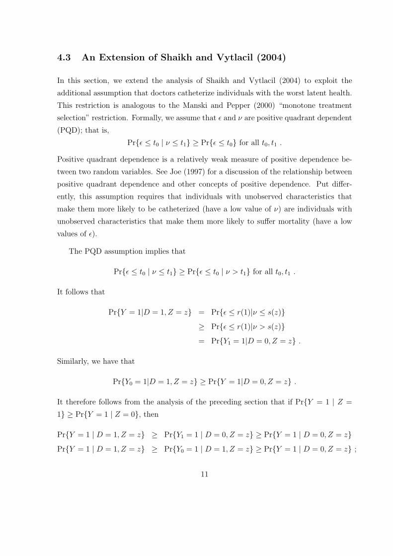
4.3 An Extension of Shaikh and Vytlacil (2004)
In this section, we extend the analysis of Shaikh and Vytlacil (2004) to exploit the
additional assumption that doctors catheterize individuals with the worst latent health.
This restriction is analogous to the Manski and Pepper (2000) “monotone treatment
selection” restriction. Formally, we assume that ǫ and ν are positive quadrant dependent
(PQD); that is,
Pr{ǫ ≤ t0 | ν ≤ t1} ≥ Pr{ǫ ≤ t0} for all t0, t1 .
Positive quadrant dependence is a relatively weak measure of positive dependence be-
tween two random variables. See Joe (1997) for a discussion of the relationship between
positive quadrant dependence and other concepts of positive dependence. Put differ-
ently, this assumption requires that individuals with unobserved characteristics that
make them more likely to be catheterized (have a low value of ν) are individuals with
unobserved characteristics that make them more likely to suffer mortality (have a low
values of ǫ).
The PQD assumption implies that
Pr{ǫ ≤ t0 | ν ≤ t1} ≥ Pr{ǫ ≤ t0 | ν > t1} for all t0, t1 .
It follows that
Pr{Y = 1|D = 1, Z = z} = Pr{ǫ ≤ r(1)|ν ≤ s(z)}≥ Pr{ǫ ≤ r(1)|ν > s(z)}= Pr{Y1 = 1|D = 0, Z = z} .
Similarly, we have that
Pr{Y0 = 1|D = 1, Z = z} ≥ Pr{Y = 1|D = 0, Z = z} .
It therefore follows from the analysis of the preceding section that if Pr{Y = 1 | Z =
1} ≥ Pr{Y = 1 | Z = 0}, then
Pr{Y = 1 | D = 1, Z = z} ≥ Pr{Y1 = 1 | D = 0, Z = z} ≥ Pr{Y = 1 | D = 0, Z = z}Pr{Y = 1 | D = 1, Z = z} ≥ Pr{Y0 = 1 | D = 1, Z = z} ≥ Pr{Y = 1 | D = 0, Z = z} ;
11

if, on the other hand, Pr{Y = 1 | Z = 1} ≤ Pr{Y = 1 | Z = 0}, then
min{Pr{Y = 1 | D = 1, Z = z},Pr{Y = 1 | D = 0, Z = z}}≥ Pr{Y1 = 1 | D = 0, Z = z} ≥ 0
max{Pr{Y = 1 | D = 1, Z = z},Pr{Y = 1 | D = 0, Z = z}}≤ Pr{Y0 = 1 | D = 1, Z = z} ≤ 1 .
These results bound Pr{Y0 = 1} and Pr{Y1 = 1}. If, for example, Pr{Y = 1 | Z = 1} >Pr{Y = 1 | Z = 0}, then
Pr{Y1 = 1} = Pr{Y1 = 1 | Z = z}= Pr{D = 1 | Z = z}Pr{Y1 = 1 | D = 1, Z = z}
+ Pr{D = 0 | Z = z}Pr{Y1 = 1 | D = 0, Z = z}≤ Pr{Y = 1 | D = 1, Z = z} ,
which implies that
Pr{Y1 = 1} ≤ minz{Pr{Y = 1 | D = 1, Z = z}} .
Using arguments given in Shaikh and Vytlacil (2004), it is possible show that
minz{Pr{Y = 1 | D = 1, Z = z}} = Pr{Y = 1 | D = 1, Z = 1} .
The bounds resulting from this line of reasoning are given by
BLPQD ≤ E[Y1 − Y0] ≤ BU
PQD ,
where
BLPQD = Pr{Y = 1 | Z = 1} − Pr{Y = 1 | Z = 0}
BUPQD = Pr{Y = 1 | D = 1, Z = 1} − Pr{Y = 1 | D = 0, Z = 0},
12

when Pr{Y = 1 | Z = 1} > Pr{Y = 1 | Z = 0},
BLPQD = Pr{D = 1, Y = 1 | Z = 1} − Pr{D = 0, Y = 1 | Z = 0}
−Pr{D = 1 | Z = 0}BU
PQD = Pr{D = 1, Y = 1 | Z = 1} + Pr{D = 0 | Z = 1}×min{Pr{Y = 1 | D = 1, Z = 1},Pr{Y = 1 | D = 0, Z = 1}}−Pr{D = 0, Y = 1 | Z = 0} − Pr{D = 1 | Z = 0}×max{Pr{Y = 1 | D = 1, Z = 0},Pr{Y = 1 | D = 0, Z = 0}} ,
when Pr{Y = 1 | Z = 1} < Pr{Y = 1 | Z = 0}, and BLPQD = BU
PQD = 0 when
Pr{Y = 1 | Z = 1} = Pr{Y = 1 | Z = 0}.
Remark 4.4 The PQD bounds are (weakly) narrower than the SV bounds. To see this,
first suppose that Pr{Y = 1 | Z = 1} > Pr{Y = 1 | Z = 0}. In this case, BLSV = BL
PQD,
but
BUSV −BU
PQD = Pr{D = 0|Z = 1} × Pr{Y = 0|D = 1, Z = 1}+ Pr{D = 1|Z = 0} × Pr{Y = 1|D = 0, Z = 0} ≥ 0 ,
so BUSV ≥ BU
PQD. Similarly, if Pr{Y = 1 | Z = 1} < Pr{Y = 1 | Z = 0}, then it is
possible to show that BUSV = BU
PQD, but BLSV ≤ BL
PQD. Typically, these inequalities
will in fact be strict. If Pr{Y = 1 | Z = 1} = Pr{Y = 1 | Z = 0}, then the average
treatment effect is identifed to be zero and the two sets of bounds coincide.
Remark 4.5 Throughout Section 4, we have assumed that there are no X covariates
and that Z is binary. Relaxing these assumptions is straightforward. If X is contained
in Z, then all of the analysis can simply be carried out conditional on X. If, on the other
hand, there exists a component of X that is not contained in Z, then it is possible to
further narrow the bounds on the average treatment effect. If there is a continuous com-
ponent of X that is not contained in Z, than it is possible to obtain point identification.
If Z is not binary, then all of the analysis can be carried out with z1 in place of 1 and z0
in place of 0, where z1 maximizes Pr{D = 1|Z = z} and z0 minimizes Pr{D = 1|Z = z}.For further details, see Shaikh and Vytlacil (2004) and Vytlacil and Yildiz (2007).
13

5 Estimation and Inference
In this section, we discuss estimation and inference for each of the bounds described in
the preceding section. We also briefly discuss a means of testing for the threshold crossing
structure on the treatment equation. For ease of exposition, we assume again that there
are no X covariates. We also assume, as in the preceding section, that Z is ordered so
that Pr{D = 1|Z = 1} > Pr{D = 1|Z = 0}. Let P denote the distribution of (Y,D,Z)
and let (Yi, Di, Zi), i = 1, . . . , n be an i.i.d. sample of random variables with distribution
P . We assume throughout that P is such that 0 < Pr{D = d, Y = y, Z = z} < 1 for all
values of (d, y, z) ∈ {0, 1}3.
5.1 Estimation
5.1.1 Bounds of Manski (1990)
Let
nz = |{1 ≤ i ≤ n : Zi = z}| (3)
and define
BLM,n = max
z
{
1
nz
∑
1≤i≤n:Zi=z
DiYi
}
− minz
{
1
nz
∑
1≤i≤n:Zi=z
((1 −Di)Yi +Di)
}
BUM,n = min
z
{
1
nz
∑
1≤i≤n:Zi=z
(DiYi + (1 −Di))
}
− maxz
{
1
nz
∑
1≤i≤n:Zi=z
(1 −Di)Yi
}
.
Clearly, BLM,n
P→ BLM and BU
M,n
P→ BUM , where BL
M and BUM are as defined in Section (4.1).
It follows that [BLM,n, B
UM,n] converges in probability to [BL
M , BUM ] under the Hausdorff
metric on subsets of R.
5.1.2 Bounds of Shaikh and Vytlacil (2004)
Let nz be given by (3) and define
∆n =
{
1
n1
∑
1≤i≤n:Zi=1
Yi −1
n0
∑
1≤i≤n:Zi=0
Yi
}
. (4)
14

Let ǫn > 0 be a sequence of numbers tending to 0, but satisfying√nǫn → ∞. Define
BLSV,n = ∆n
BUSV,n =
{
1
n1
∑
1≤i≤n:Zi=1
(DiYi + (1 −Di)) −1
n0
∑
1≤i≤n:Zi=0
(1 −Di)Yi
}
when ∆n > ǫn,
BLSV,n =
{
1
n1
∑
1≤i≤n:Zi=1
DiYi −1
n0
∑
1≤i≤n:Zi=0
((1 −Di)Yi +Di)
}
BUSV,n = −∆n
when ∆n < −ǫn, and BLSV,n = BU
SV,n = 0 when |∆n| ≤ ǫn. Clearly, BLSV,n
P→ BLSV
and BUSV,n
P→ BUSV , where BL
SV and BUSV are as defined in Section 4.2. It follows that
[BLSV,n, B
USV,n] converges in probability to [BL
SV , BUSV ] under the Hausdorff metric on sub-
sets of R.
5.1.3 PQD Bounds
Let nz be given by (3) and define
nz,d = |{1 ≤ i ≤ n : Zi = z,Di = d}| . (5)
Let ∆n be given by (4), and let ǫn > 0 be a sequence of numbers tending to 0, but
satisfying√nǫn → ∞. Define
BLPQD,n = ∆n
BUPQD,n =
{
1
n1,1
∑
1≤i≤n:Zi=1,Di=1
Yi −1
n0,0
∑
1≤i≤n:Zi=0,Di=0
Yi
}
15

when ∆n > ǫn,
BLPQD,n =
{
1
n1
∑
1≤i≤n:Zi=1
DiYi −1
n0
∑
1≤i≤n:Zi=0
((1 −Di)Yi +Di)
}
BUPQD,n =
1
n1
∑
1≤i≤n:Zi=1
DiYi +1
n1
∑
1≤i≤n:Zi=1
(1 −Di)
×min
{(
1
n1,1
∑
1≤i≤n:Zi=1,Di=1
Yi
)
,
(
1
n1,0
∑
1≤i≤n:Zi=1,Di=0
Yi
)}
− 1
n0
∑
1≤i≤n:Zi=0
(1 −Di)Yi −1
n0
∑
1≤i≤n:Zi=0
Di
×max
{(
1
n0,1
∑
1≤i≤n:Zi=0,Di=1
Yi
)
,
(
1
n0,0
∑
1≤i≤n:Zi=0,Di=0
Yi
)}
when ∆n < −ǫn, and BLPQD,n = BU
PQD,n = 0 when |∆n| ≤ ǫn. Again, BLPQD,n
P→ BLPQD
and BUPQD,n
P→ BUPQD. It follows that [BL
PQD,n, BUPQD,n] converges in probability to
[BLPQD, B
UPQD] under the Hausdorff metric on subsets of R.
Remark 5.1 The above estimators for the Shaikh and Vytlacil (2004) bounds and the
PQD bounds have some obvious drawbacks. Both are superefficient when the average
treatment effect is in fact equal to zero, which suggests that they would behave poorly
in a neighborhood of zero. Moreover, for a given sample of size n, there is no restriction
on the level of ǫn. As a result, in the next section, we focus instead on constructing
confidence sets for the average treatment effect, which do not suffer from such undesirable
features.
Remark 5.2 Unlike the Manski (1990) bounds, the Shaikh and Vytlacil (2004) bounds
and the PQD bounds in general cannot be estimated consistently simply by replacing
conditional population means with conditional sample means. This is because these
bounds are both discontinuous as a function of Pr{Y = 1|Z = 1} − Pr{Y = 1|Z = 0}.In particular, it is not possible to set ǫn = 0 and maintain consistency of the estimators.
To see this, simply note that when Pr{Y = 1|Z = 1} − Pr{Y = 1|Z = 0} = 0, the
events ∆n > 0 and ∆n < 0 each have probability 1/2 asymptotically.
16

5.2 Inference
In this section, we construct random sets Cn such that for each θ between the upper and
lower bounds
lim infn→∞
Pr{θ ∈ Cn} ≥ 1 − α . (6)
Such confidence sets have been termed by Romano and Shaikh (2006) as confidence
regions for identifiable parameters.
Following Romano and Shaikh (2006), our construction will be based upon test
inversion. For each −1 ≤ θ ≤ 1, we will construct a test of the null hypothesis that θ
lies between the upper and lower bounds. The confidence region Cn will then simply be
defined to the set of values for θ for which we fail to reject the corresponding test of the
null hypothesis. Concretely, define
Cn = {−1 ≤ θ ≤ 1 : Tn(θ) ≤ cn(θ, 1 − α)} , (7)
where Tn(θ) is a test statistic for which large values provide evidence against the null
hypothesis and cn(θ, 1−α) is an appropriate critical value. The critical value cn(θ, 1−α)
will be constructed using subsampling. In order to describe the construction, we require
some further notation. Let b = bn < n be a sequence of positive integers tending to
infinity, but satisfying bn/n → 0. Index by i = 1, . . . , Nn =(
n
b
)
the different subsets of
{1, . . . , n} of size b. Denote by Tn,b,i(θ) the test statistic Tn(θ) computed using only the
ith subset of data of size b. Let cn(θ, 1 − α) denote the (smallest) 1 − α quantile of the
distribution
Ln(x, θ) =1
Nn
∑
1≤i≤Nn
I{Tn,b,i(θ) ≤ x} . (8)
Romano and Shaikh (2006) show that Cn defined by (7) satisfies the coverage property
(6) under weak conditions on the distribution of Tn(θ) under P . In each of the appli-
cations below, it is straightfoward to show that these conditions hold using arguments
similar to those given in Section 3.2 of Romano and Shaikh (2006).
17

5.2.1 Bounds of Manski (1990)
Let nz be given by (3) and let z = (z1, z2, z3, z4). Define
δ1,n(z1, z2) =1
nz1
∑
1≤i≤n:Zi=z1
DiYi −1
nz2
∑
1≤i≤n:Zi=z2
((1 −Di)Yi +Di)
δ2,n(z1, z2) =1
nz3
∑
1≤i≤n:Zi=z1
(DiYi + (1 −Di)) −1
nz4
∑
1≤i≤n:Zi=z2
(1 −Di)Yi
Denote by σ({Wi : 1 ≤ i ≤ n}) the usual estimate of the standard deviation of the
random variables Wi, i = 1, . . . , n. If z1 6= z2, then define
s1,n(z1, z2) =
√
γ1,n(z1)
nz1
+γ2,n(z2)
nz2
s2,n(z1, z2) =
√
γ3,n(z1)
nz1
+γ4,n(z2)
nz2
,
where
γ1,n(z1) = σ({DiYi : Zi = z1, 1 ≤ i ≤ n})γ2,n(z1) = σ({(1 −Di)Yi +Di : Zi = z1, 1 ≤ i ≤ n})γ3,n(z1) = σ({DiYi + (1 −Di) : Zi = z1, 1 ≤ i ≤ n})γ4,n(z1) = σ({(1 −Di)Yi : Zi = z1, 1 ≤ i ≤ n}) ;
if z1 = z2, then define
s1,n(z1, z2) =σ({DiYi − (1 −Di)Yi −Di : Zi = z1, 1 ≤ i ≤ n})
√nz1
s2,n(z1, z2) =σ({DiYi + (1 −Di) − (1 −Di)Yi : Zi = z1, 1 ≤ i ≤ n})
√nz1
.
For −1 ≤ θ ≤ 1, define
Tn(θ) =∑
z∈{0,1}4
{
(
δ1,n(z1, z2) − θ
s1,n(z1, z2)
)2
+
+
(
θ − δ2,n(z3, z4)
s2,n(z3, z4)
)2
+
}
,
where (x)+ = max{x, 0}.
18

Remark 5.3 Imbens and Manski (2004) provide confidence regions with the coverage
property (6) for partially identified models where the identified set is an interval whose
upper and lower endpoints are means or at least behave like means asymptotically.
Although the identified set here is also an interval, the upper and lower endpoints do
not have this property, so their analysis is not applicable here.
5.2.2 Bounds of Shaikh and Vytlacil (2004)
Let ∆n be given by (4) and define
sn =
√
σ({Yi : Zi = 1, 1 ≤ i ≤ n})n1
+σ({Yi : Zi = 0, 1 ≤ i ≤ n})
n0
. (9)
For 0 < θ ≤ 1, define
Tn(θ) =
(−∆n
sn
)2
+
+
(
∆n − θ
sn
)2
+
+
(
θ − δ2,n(1, 0)
s2,n(1, 0)
)2
+
;
for −1 ≤ θ < 0, define
Tn(θ) =
(
∆n
sn
)2
+
+
(
θ − ∆n
sn
)2
+
+
(
δ1,n(1, 0) − θ
s1,n(1, 0)
)2
+
;
and for θ = 0, define
Tn(θ) =
(
∆n
sn
)2
.
5.2.3 PQD Bounds
Let nz,d be given by (5), let ∆n be given by (4), and let sn be given by (9). Define
δ3,n =1
n1,1
∑
1≤i≤n:Zi=1,Di=1
Yi −1
n0
∑
1≤i≤n:Zi=0
Yi
δ4,n =1
n1,1
∑
1≤i≤n:Zi=1,Di=1
Yi −1
n0,0
∑
1≤i≤n:Zi=0,Di=0
Yi
δ5,n =1
n1
∑
1≤i≤n:Zi=1
Yi −1
n0,0
∑
1≤i≤n:Zi=0,Di=0
Yi ,
19

and
s3,n =
√
σ({Yi : Zi = 1, Di = 1, 1 ≤ i ≤ n})n1,1
+σ({Yi : Zi = 0, 1 ≤ i ≤ n})
n0
s4,n =
√
σ({Yi : Zi = 1, Di = 1, 1 ≤ i ≤ n})n1,1
+σ({Yi : Zi = 0, Di = 0, 1 ≤ i ≤ n})
n0,0
s5,n =
√
σ({Yi : Zi = 1, 1 ≤ i ≤ n})n1
+σ({Yi : Zi = 0, Di = 0, 1 ≤ i ≤ n})
n0,0
.
For 0 < θ ≤ 1, define
Tn(θ) = (−∆n
sn
)2+ + (
∆n − θ
sn
)2+ +
(
θ − δ4,n
s4,n
)2
+
;
for −1 ≤ θ < 0, define
Tn(θ) =
(
∆n
sn
)2
+
+
(
δ1,n(1, 0) − θ
s1,n(1, 0)
)2
+
+
(
θ − δ3,n
s3,n
)2
+
+
(
θ − δ4,n
s4,n
)2
+
+
(
θ − ∆n
sn
)2
+
+
(
θ − δ5,n
s5,n
)2
+
;
and for θ = 0, define
Tn(θ) =
(
∆n
sn
)2
.
5.3 A Test of Threshold Crossing
As discussed in Remark 4.2, Heckman and Vytlacil (2001) show that when D is given
by (2) and that the unobservables are independent of Z the bounds of Manski (1990)
may be written as
BLM = Pr{D = 1, Y = 1|Z = 1} − Pr{D = 0, Y = 1|Z = 0} − Pr{D = 1 | Z = 0}
BUM = Pr{D = 1, Y = 1|Z = 1} + Pr{D = 0 | Z = 1} − Pr{D = 0, Y = 1|Z = 0} .
It is therefore possible to test whether D is given by (2) and that the unobservables are
independent of Z by comparing these expressions for the bounds of Manski (1990) with
those stated in equation (4.1). These two expressions will be the same if and only if
Pr{D = 0, Y = 1|Z = 1} − Pr{D = 1 | Z = 1} ≥Pr{D = 0, Y = 1|Z = 0} − Pr{D = 1 | Z = 0}
20

Pr{D = 1, Y = 1|Z = 0} + Pr{D = 0 | Z = 0} ≥Pr{D = 1, Y = 1|Z = 1} + Pr{D = 0 | Z = 1}
Pr{D = 1, Y = 1|Z = 1} ≥ Pr{D = 1, Y = 1|Z = 0}Pr{D = 0, Y = 1|Z = 0} ≥ Pr{D = 0, Y = 1|Z = 1} .
We now describe one of several possible ways of testing whether these inequalities hold
jointly. Let nz be given by (3) and define
ψ1,n =1
n0
∑
1≤i≤n:Zi=0
((1 −Di)Yi −Di) −1
n1
∑
1≤i≤n:Zi=1
((1 −Di)Yi −Di)
ψ2,n =1
n1
∑
1≤i≤n:Zi=1
(DiYi + (1 −Di)) −1
n0
∑
1≤i≤n:Zi=0
(DiYi + (1 −Di))
ψ3,n =1
n0
∑
1≤i≤n:Zi=0
DiYi −1
n1
∑
1≤i≤n:Zi=1
DiYi
ψ4,n =1
n1
∑
1≤i≤n:Zi=1
(1 −Di)Yi −1
n0
∑
1≤i≤n:Zi=0
(1 −Di)Yi .
Consider the test statistic Tn =∑
1≤i≤4(ψi,n)2+ . Large values of this test statistic provide
evidence against the null hypothesis that all four of the above inequalities hold. We may
again construct a critical value for this test statistic using subsampling as described in
the beginning of Section 5.2. The validity of such an approach can be verified as before
using arguments similar to those given in Section 3.2 of Romano and Shaikh (2006).
One may, of course, also divide each of the ψi,n by its standard error, as was done for
the test statistics in the previous sections.
6 Data
The Connors et al. (1996) data come from ICUs at five prominent hospitals – Duke
University Medical Center, Durham, NC; MetroHealth Medical Center, Cleveland, OH;
St. Joseph’s Hospital, Marshfield, WI; and University of California Medical Center, Los
Angeles, CA. The study admitted only severely ill patients with one of nine disease
conditions: acute respiratory failure, chronic obstructive pulmonary disease, congestive
21

heart failure, cirrhosis, nontraumatic coma, metastatic colon cancer, late-stage non-small
cell lung cancer, and multiorgan system failure with malignancy or sepsis. 59.2% of the
sample is over the age of 60. Murphy and Cluff (1990) provide a detailed description
of patient recruitment procedures, including a list of exclusion criteria. Connors et al.
(1996) count a patient as catheterized if the procedure was performed within 24 hours
of entering the ICU.
There are 5,735 patients, all of whom were admitted to or transferred to the ICU
within 24 hours of entering the hospital. Connors et al. (1996) collected a large amount
of information about each patient via standardized medical chart abstraction methods
and interviews with patients and patient surrogates. Tables 1 - 3 compare patients who
were catheterized during their first day of admission to the ICU with those who were
not catheterized. These tables present the p-value from a test of the hypothesis that the
means of the variables are equal for catheterized and non-catheterized patients.
Table 1 compares patients on the basis of demographic variables and the primary
diagnosis at admission. Catheterized patients are more likely to be male (by 4.2%),
privately insured (by 6.1%), richer (less likely to have an income of less than $11,000 per
year by 5.5%), and have more schooling (0.2 years more on average). Of the patients
in our sample, 60.9% of non-catheterized patients had a primary diagnosis of acute
respiratory failure, while only 46% of our catheterized patients had the same diagnosis.
Table 2 compares patients on the basis of disease history prior to admission and
functional status. Catheterized patients are more likely to have had a diagnosis of cardiac
disease (by 1.9%), congestive heart failure (by 2.0%), or acute myocardial infarction
(by 1.2%) in their medical history. Catheterized patients also have a 3.3% lower two
month predicted survival rate upon admission than non-catheterized patients – clearly
catheterized patients are observably more ill than non-catheterized patients.
Table 3 compares catheterized and non-catheterized patients’ laboratory values at
admission, as well as any secondary diagnoses these patients may have had at admission.
Among the laboratory values, all the clinically significant and interpretable differences
point toward the conclusion that catheterized patients are observably sicker.
Remark 6.1 Because of the large number of comparisons we are making, it is likely
22

that we will reject several hypotheses falsely. We use the multiple testing procedure of
Holm (1979) to make the comparisons while controlling the familywise error rate – the
probability of even one false rejection – at level α. Let p(1) ≤ . . . ≤ p(s) denote the ordered
values of the p-values and let H(1), . . . , H(s) denote the corresponding null hypotheses.
If p(1) ≥ α/s, then the procedure rejects no null hypotheses; otherwise, it rejects null
hypotheses H(1), . . . , H(r), where r is the largest index such that p(i) ≤ α/(s−i+1) for all
i ≤ r. This procedure always rejects at least as many null hypotheses as the Bonferroni
procedure, which simply rejects any null hypothesis Hi for which the corresponding
pi ≤ α/s.
At level α = .05, we find that patients who are catheterized differ from those who are
not catheterized along 32 of 60 possible variables. The results are qualitatively similar
at level α = .01. Hence, even after accounting for the multiplicity of comparisons, we
maintain our earlier conclusion that catheterized patients are significantly different than
non-catheterized patients.
7 Instrumenting with Admission Day
A direct comparison of outcomes between catheterized and non-catheterized patients
is unlikely to yield the causal effects of catheterization. Even if a full set of controls
were included in the analysis, the results would be unconvincing. If catheterized and
non-catheterized patients differ on so many observed dimensions, it is unlikely that they
do not differ on unobserved dimensions as well. See Altonji et al. (2005) for a formal
justification of this argument. In this section, we develop suggestive evidence that day-
of-the-week of admission is an appropriate instrument to determine the causal effect of
catheterization on patient mortality.
7.1 Admission Day of Week Predicts Catheterization
We first establish that patients who are admitted to the ICU on a Saturday, Sunday,
or Monday are substantially less likely to be catheterized on the day of admission than
patients admitted on other days of the week. The results remain similar if we exclude
23

Monday from the definition of the weekend. Figure 1 shows catheterization rates by
day-of-the-week for four important clinical groups, based on primary diagnosis upon
ICU admission. For all four groups, the probability of being catheterized decreases on
weekends. A t-test of the difference in probability of catheterization between weekend
and weekday rejects equality at 0.05 level for all four groups. However, the same is not
true for patients with chronic obstructive pulmonary disease (COPD), cirrhosis, coma,
and lung cancer: there is no statistically significant difference, so we drop patients from
these groups from all subsequent analysis.
7.2 Patient Health and Day of Week of Admission
If patients admitted to the ICU on a weekday differed systematically from patients
admitted on weekends, then day-of-the-week would be a poor instrument since it would
be correlated with unobserved determinants of ICU patient mortality such as health
status. We believe that there should be no such correlation, since the health crises that
precipitate ICU admissions are unlikely to respect distinctions between weekdays and
weekends. We now present suggestive evidence in favor of this view.
Tables 4 - 6 divide patients into two groups on the basis of the instrument: those
who were admitted on a weekday and those who were admitted on a weekend. The
tables present mean values of each variable on which we make comparisons, along with
standard deviations of those variables and the p-value from a test of the hypothesis that
the means of the variables are equal.
Table 4 compares patients based on demographic variables on the primary diagnosis.
We find no statistically significant differences between patients admitted on a weekend
and those admitted on a weekday when testing at the α = 0.01 level. Similarly Ta-
ble 5, which compares patients based on disease history and functional status, shows no
statistically significant differences between weekend and weekday patients. Importantly,
there is little difference between these groups in predicted 2-month mortality, or in acute
physiology score. Finally, Table 6 compares weekend and weekday patients on the basis
of laboratory tests at admission and on secondary diagnoses. There are no statistically
significant differences between the two groups on these bases.
24

Remark 7.1 We could apply the multiple testing procedure of Holm (1979) to make
the comparisons while controlling the familywise error rate at level α, but it suffices to
note that the multiple testing procedure will never reject more null hypotheses than the
naive testing procedure above. Therefore, even after accounting for the multiplicity of
comparisons, we find that there are no statistically significant differences between the
two groups.
Remark 7.2 Even though health status at admission does not appear to vary by the day
of week of admission to the ICU, the death rates will vary if catheterization rates depend
on day of week of admission and mortality is effected by catheterization. Figure 2 shows
mean mortality rates at 7, 30, 60, 90, and 180 days after ICU admission for patients
admitted on weekends and weekdays as well as 95% confidence intervals around the
means. At 30, 60, 90, and 180 days post-ICU admission, mortality rates are significantly
higher at level α = 0.05 for patients admitted on weekdays than patients admitted on
weekends.
7.3 Day of Week, Hospital Staffing, and Outcomes
Although non-specialists sometimes find it surprising, it is well known in the health
services literature that medical staffing can have a major effect on treatment decisions,
including the decision to catheterize a patient. Rapoport et al. (2000), for example,
find that patients admitted to ICUs that staff a full time ICU physician are two-thirds
less likely to be catheterized than those admitted to ICUs with no full time physi-
cian. Whether this fact threatens the validity of our instrument depends upon whether
there are unobserved differences in treatment between weekday and weekend admis-
sions, unassociated with catheterization, that help determine patient mortality. If so,
then admission day would not be a valid instrument.
Evaluating the importance of differences in treatment between weekend and weekday
admissions is complicated by the fact that Swan-Ganz catheterization itself is a gateway
to a large number of other treatments. For example, ICU physicians often use the
information from catheterization to titrate the dose of inotropic drugs, such as dopamine
and dobutamine, which are designed to improve cardiac contractility. These drugs have
25

a narrow therapeutic range, and thus getting the dose right can be the difference between
killing or inadequately treating a patient. Since catheterization is less likely on weekends,
it would be unsurprising to find decreased use of inotropes on weekends as well. We can
accommodate such differences in treatment between weekend and weekday admissions
by simply reinterpreting the treatment as catheterization and all the other treatments it
enables or encourages on mortality, rather than catheterization by itself.
It is possible that weekend-weekday staffing differences, for reasons having nothing
to do with catheterization or its downstream consequences, may lead to higher patient
mortality. If so, then our instrument would be invalid. Since staffing tends to be sparser
on weekends, one would expect that mortality rates would be higher then. In fact, in our
data mortality rates are higher on weekdays, which is inconsistent with a direct mortality
effect of staffing. Furthermore, several studies have found no evidence that staffing
differences explain weekend-weekday mortality differences in ICUs–see Ensminger et al.
(2004), Wunsch et al. (2004), and Dobkin (2003).
8 Results
In this section, we first follow the traditional approach of estimating parametric models
that allow us to identify the average treatment effect. In particular, we consider linear
models and bivariate probit models. We then report results from the three different
bounds described in Section 4.
We analyze outcomes t days after admission to the ICU separately for different values
of t – 7, 30, 60, 90, and 180 days. For this reason, we write the outcome Y and the
potential outcomes Y0 and Y1 as functions of t throughout the remainder of the paper.
8.1 Parametric Models
The panel on the righthand side of Figure 3 shows estimates of the coefficient on D
and associated 95% confidence intervals obtained from ordinary least squares (OLS)
regression of Y (t) on a constant and D for the different values of t. The panel on the
lefthand side shows estimates of the coefficient on D and associated 95% confidence
26

intervals obtained from OLS regression of Y (t) on a constant, D and the full set of
covariates listed in Tables 1 - 3 for the different values of t. For these estimates to
be consistent for the average treatment effect, we require that the treatment D be
independent of the potential outcomes Y0(t) and Y1(t) (conditional on covariates) and
that the linear model underlying the regression is correct. Under these assumptions,
one might conclude from these results that excess mortality due to catheterization 7
days after ICU admission is about two percentage points and it increases to about six
percentage points 30 days after admission.
Even if these assumptions are correct, a possible problem with these results is that
they ignore the possibility that catheterized patients differ in unobserved ways from non-
catheterized patients. For this reason, we may consider maximum likelihood estimation
of the bivariate probit model described in Remark 3.2. The bivariate probit model is a
common approach in the context of a dummy endogenous regressor as a determinant of
a binary outcome; see, for example, Goldman et al. (2001). For the sake of brevity, we
report only the results without X regressors.
Figure 4 shows 95% confidence intervals around the average treatment effect E[Y1(t)−Y0(t)] from maximum likelihood estimation of the bivariate probit model for the different
values of t. Like the OLS results, the bivariate probit results suggest that catheterization
increases mortality rates at 30, 60, 90, and 180 days after ICU admission. Like the OLS
results without covariates but unlike the OLS results with covariates, the confidence
interval for the average treatment effect crosses zero at 7 days.
Although the bivariate probit model allows catheterized and non-catheterized pa-
tients to differ in unobserved ways, it still requires many strong, parametric assumptions.
We therefore consider the three nonparametric bounds described in Section 4
8.2 Nonparametric Bounds
We consider each of the three bounds described in Section 4. Each of these bounds rely
upon our instrumental variable – an indicator for whether the patient was admitted to the
ICU on a Tuesday - Friday. For each of the bounds, we display 95% confidence intervals
for the average treatment effect computed as described in Section 5. Computational
27

details are described below in Remark 8.4. The lefthand side of Figure 5 shows the
bounds of Manski (1990) for the whole sample, whereas the righthand side shows the
bounds of Shaikh and Vytlacil (2004) for the whole sample. The Manski (1990) bounds
have a width of nearly one and thus always fail to exclude zero; see Remark 8.1 below for
further discussion. The Shaikh and Vytlacil (2004) bounds, by contrast, are considerably
more informative: at 7 days after ICU admission, these bounds include zero; but at 30
days after admission to the ICU and beyond, the bounds suggest that catheterization
increases mortality. The width of the these bounds are about half the width of the
Manski (1990) bounds.
Recall that Connors et al. (1996) found that catheterization increases mortality even
at 7 days using this same data set that we use here, but a different statistical method
that assumes that there are no unobserved differences between catheterized and non-
catheterized patients. Their result raises the question of why ICU doctors do not observe
the increased mortality from catheterization and react accordingly. The Shaikh and
Vytlacil (2004) bounds provides a possible answer – ICU doctors do not see rise in
mortality which happens only after many patients have been released from the ICU.
Figure 6 shows the bounds from the extension of Shaikh and Vytlacil (2004) described
in Section 4.3. These bounds impose the restriction that doctors are effective at triaging
patients so that it is those patients with the worst health who are actually catheterized.
These figures show that imposing this plausible restriction decreases the width of the
treatment effect bounds, often dramatically.
By construction, these bounds are always on the same side of zero as the Shaikh
and Vytlacil (2004) bounds. The reduction in the width of the bounds is greatest when
the average treatment effect is positive; that is, when catheterization increases mortality.
This is to be expected, as the PQD restriction rules out the possibility that doctors cause
great harm to large numbers of their patients. On the other hand, the PQD bounds
have a lower upper bound than the Shaikh and Vytlacil (2004) bounds when the average
treatment effect is negative, that is, when catheterization decreases mortality, so it may
permit researchers to conclude, for example, that the inverntion is cost-effective even as
the Shaikh and Vytlacil (2004) bounds permit the possibility that it may not be.
28

Remark 8.1 Despite the evidence presented in Section 7, it is interesting to consider
how our inferences would change if we did not rely upon our instrumental variable. One
possible answer is to rely on the bounds of Manski (1990), which may be constructed
without an instrument. In that case, the width of the bounds is always exactly one
and thus always fail to exclude zero. A second possible answer is given by the analysis
of Section 4.3, which may also be constructed without an instrument. In that case,
the PQD assumption reduces to Pr{Y1 = 1 | D = 1} ≥ Pr{Y1 = 1 | D = 0} and
Pr{Y0 = 1 | D = 1} ≥ Pr{Y0 = 1 | D = 0}, which implies the following bounds on the
average treatment effect:
Pr{Y1 = 1 | D = 1}Pr{D = 1} − Pr{Y0 = 1 | D = 0}Pr{D = 0} − Pr{D = 1}≤ E[Y1 − Y0] ≤ Pr{Y1 = 1 | D = 1} − Pr{Y0 = 1 | D = 0}
Figure 7 shows these bounds and associated 95% confidence intervals. In every case,
the bounds cross zero, though their width is substantially less than one. The PQD
assumption by itself is therefore not enough to identify the direction of the treatment
effect.
Remark 8.2 Heckman and Vytlacil (2001) show that the threshold crossing structure
implies that BUM −BL
M = 1−Pr{D = 1|Z = 1}+ Pr{D = 1|Z = 0}, where Z is ordered
such that Pr{D = 1|Z = 1} > Pr{D = 1|Z = 0}. If Pr{D = 1|Z = 1} is close to
one and Pr{D = 1|Z = 0} is close to zero, then the bounds will have width close to
zero. In contrast, if Pr{D = 1|Z = 1} is close to Pr[D = 1|Z = 0}, the width of the
bounds will be nearly one, i.e., almost as wide as the naive bounds that do not impose
or exploit an instrument described in Remark 8.1. Our empirical result that the width
of the bounds is close to one is a direct result of the instrument being weak in the sense
that Pr{D = 1|Z = 1} is close to Pr{D = 1|Z = 0}. This is a separate issue from the
question of whether the instrument is highly statistically significant in the propensity
score model. As we discuss in Section 7.1, for the patient groups we analyze, we can
reject that Pr{D = 1|Z = 1} = Pr{D = 1|Z = 0}. Furthermore, in the bivariate probit
model reported above, a test of the significance of the instruments in the catheterization
equation rejects that the coefficient on the instruments are jointly zero at p = 0.0072 for
the model where the main outcome is 30 day mortality.
29

Remark 8.3 We also implement the test of the threshold crossing assumption that is
described in Section 5.3. At the α = 0.10 level and for each value of t we fail to reject
the inequalities shown in that section, providing evidence in favor of the assumptions
underlying the bounds described in Sections 4.2 and 4.3.
Remark 8.4 For the results we reported above, we used a subsample size of b = 50. In
results not reported here, we also tried different subsample sizes ranging from 25 to 75
and found that our results are remained similar for these values of b. Finally, because Nn
is large, we used an approximation to (8) in which we randomly chose with replacement
Bn = 1000 of the Nn possible subsamples. It follows from Corollary 2.4.1 of Politis et al.
(1999) that critical values constructed in this way remain valid provided that Bn tends
to infinity.
9 Conclusion
While direct comparisons of the mortality of catheterized and non-catheterized patients
lead to the conclusion that catheterization increases mortality, we show evidence that
this result is due to profound differences between the catheterized and non-catheterized
patients; the former are much more severely ill than the latter.
We provide suggestive evidence that weekday admission can serve as an instrumental
variable for catheterization. Patients admitted on a weekday are about four to eight
percentage points more likely to be catheterized than patients admitted on a weekend.
Yet, weekday and weekend patients appear similar in health status along a large number
of dimensions. Exploiting an instrumental variable permits us to address the unobserved
differences between catheterized and non-catheterized ICU patients.
We turn to bounding approaches that exploit access to our instrument, including
the recent approach introduced by Shaikh and Vytlacil (2004), which we compare with
the approach of Manski (1990). We find that, while the Manski (1990) bounds always
straddle zero, the Shaikh and Vytlacil (2004) bounds typically produces a clearer answer
– catheterization increases mortality at 30 days and beyond, while at 7 days the average
treatment effect may be zero. We extend the analysis of Shaikh and Vytlacil (2004)
30

to exploit a further nonparametric structural assumption – that doctors catheterize
individuals with systematically worse latent health – and find that this assumption
further narrows these bounds and strengthens these conclusions.
The main theme of the paper is the trade-off induced by the acceptance of potentially
unverifiable structural assumptions. If one is willing to accept very strong structural
assumptions, such as those underlying the bivariate probit model, one obtains point
identification. At the other extreme, if the only structural assumption one accepts is that
probabilities lie between zero and one (such as in the Manski (1990) bounds without an
instrument), then the width of the bounds on the average treatment effect is exactly one,
so it is not possible to determine the sign of the average treatment effect. In between
these two extremes, one may accept different nonparametric, structural assumptions,
such as the validity of an instrument or threshold crossing models on the outcome or
treatment variables, which may not lead to point identification, but may reduce the
width of the bounds considerably, as in our empirical example, and are more palatable
than the very strong parametric assumptions required for the bivariate probit model.
Our primary substantive finding is that catheterization improves mortality outcomes
only in the short run, if at all, and increases it in the long run. This finding is intuitively
appealing because it suggests a possible explanation for the fact that many ICU doctors
are committed to the use of the Swan-Ganz catheter. Since most ICU patients leave the
ICU well before 30 days after admission have elapsed, ICU doctors may never observe
the increase in mortality. Our results also suggest a second (not mutually exclusive)
possibility: a simple selection story. Catheterization saves the lives, in the short run, of
the most severely ill patients, but the deaths of these patient cannot be staved off for
long. Disentangling these possibilities will require even more detailed data and further
research.
31

A Comparison to Manski and Pepper (2000)
We now compare the assumptions and resulting bounds of Shaikh and Vytlacil to the
assumptions and resulting bounds of Manski and Pepper (2000). Manski and Pepper
(2000) consider several restrictions, including the “monotone instrumental variables”
assumption with a “monotone treatment response” (MTR) assumption. The MTR as-
sumption is that one knows a priori that Y1 ≥ Y0 for all individuals or one knows a
priori that Y0 ≥ Y1 for all individuals. In comparison, our analysis identifies the sign
of the average treatment effect from the data and does not impose it a priori. On the
other hand, our analysis imposes the threshold crossing model on D and Y , while no
such assumption is imposed by Manski and Pepper (2000).
For ease of exposition, suppose Z is binary and order Z so that Pr{D = 1|Z = 1] >
Pr{D = 1|Z = 0]. Consider the case of no X regressors and the bounds that would
result from applying the analysis of Manski and Pepper (2000) with MTR with Y1 ≥ Y0
and the instrumental variable (IV) assumption of Manski (1990) that Y1 and Y0 are
independent of Z.
Define
Q1(z) = Pr{Y = 1|Z = z}Q2(z) = Pr{D = 1, Y = 1|Z = z} + Pr{D = 0|Z = z}Q3(z) = Pr{D = 0, Y = 1|Z = z} .
It follows from the analysis of Proposition 2 of Manski and Pepper (2000) that MTR
with Y1 ≥ Y0 and IV jointly imply
max{Q1(0), Q1(1)} ≤ E[Y1] ≤ min{Q2(0), Q2(1)}max{Q3(0), Q3(1)} ≤ E[Y0] ≤ min{Q1(0), Q1(1)} .
In general, these bounds do not simplify without further restrictions than those imposed
by Manski and Pepper (2000); that is, one cannot know which value of z the respective
maximums and minimums are obtained at which value of z even with our ordering that
Pr{D = 1|Z = 1} > Pr{D = 1|Z = 0}. However, under the assumptions of Section
3, it follows from the analysis of Theorem 2 of Heckman and Vytlacil (2001) that their
32

bounds simplify to
Q1(1) ≤ E[Y1] ≤ Q2(1)
Q3(0) ≤ E[Y0] ≤ Q1(0) ,
so that
Q1(1) −Q1(0) ≤ E[Y1 − Y0] ≤ Q2(1) −Q3(0) .
The bounds therefore coincide with the Shaikh and Vytlacil (2004) bounds given in
equation (4.2), which hold if Shaikh and Vytlacil (2004) infer that Y1 ≥ Y0 from Pr{Y =
1|Z = 1} − Pr{Y = 1|Z = 0} > 0. Likewise, consider the Manski and Pepper bounds
that impose MTR with Y1 ≤ Y0 and IV. Under the assumptions of Section 3, the form of
the Manski and Pepper (2000) bounds simplify to the Shaikh and Vytlacil (2004) bounds
given in equation (4.2), which hold if Shaikh and Vytlacil (2004) infer that Y1 ≤ Y0 from
Pr{Y = 1|Z = 1} − Pr{Y = 1|Z = 0} < 0.
It might seem natural that one could follow the Manski and Pepper (2000) analysis
without imposing a priori that one knew the sign of the treatment response but instead
inferring it from the data from the sign of Pr{Y = 1|Z = 1} − Pr{Y = 1|Z = 0} in
the same manner as is done by the Shaikh and Vytlacil (2004). Under their conditions,
however, there is no necessary connection between the sign of the treatment response
and the sign of Pr{Y = 1|Z = 1} − Pr{Y = 1|Z = 0}.1 To see this, consider imposing
only their assumptions without imposing the additional structure of Shaikh and Vytlacil
(2004). Let D1 denote the counterfactual choice variable corresponding to Z = 1, and
let D0 denote the counterfactual choice variable corresponding to Z = 0. Suppose
Z ⊥⊥ (Y0, Y1, D0, D1) and that Y1 ≥ Y0. It is possible to show that
Pr{Y = 1|Z = 1} − Pr{Y = 1|Z = 0}= Pr{Y1 > Y0} (Pr{D1 = 1, D0 = 0|Y1 > Y0} − Pr{D1 = 0, D0 = 1|Y1 > Y0}) ,
while
Pr{D = 1|Z = 1} − Pr{D = 1|Z = 0}= Pr{Y1 > Y0} (Pr{D1 = 1, D0 = 0|Y1 > Y0} − Pr{D1 = 0, D0 = 1|Y1 > Y0})
+ Pr{Y1 = Y0} (Pr{D1 = 1, D0 = 0|Y1 = Y0} − Pr{D1 = 0, D0 = 1|Y1 = Y0}) .1Imbens and Angrist (1994) also show that it is possible to have Y1 ≥ Y0 for all individuals and yet
have a negative probability limit for the instrumental variables estimand.
33

Thus, if it is the case that
Pr{D1 = 1, D0 = 0|Y1 > Y0} < Pr{D1 = 0, D0 = 1|Y1 > Y0}Pr{D1 = 1, D0 = 0|Y1 = Y0} < Pr{D1 = 0, D0 = 1|Y1 = Y0} ,
then it is possible to have Pr{D = 1|Z = 1} − Pr{D = 1|Z = 0} > 0 while Pr{Y =
1|Z = 1} − Pr{Y = 1|Z = 0} < 0 even though Y1 ≥ Y0 for all individuals. Parallel
reasoning shows that it is possible to have Pr{D = 1|Z = 1} − Pr{D = 1|Z = 0} > 0
while Pr{Y = 1|Z = 1}−Pr{Y = 1|Z = 0} > 0 even though Y1 ≤ Y0 for all individuals.
Hence, under the assumptions of Manski and Pepper (2000), the sign of the treatment
response must be imposed a priori and cannot be inferred from the sign of Pr{Y =
1|Z = 1} − Pr{Y = 1|Z = 0} as in Shaikh and Vytlacil (2004).
By Vytlacil (2002), the assumptions of Shaikh and Vytlacil (2004) are equivalent
to imposing monotonicity of Y in D and of D in Z. Thus, another way to state this
contrast is that imposing monotonicity of Y in D is not enough to allow one to recover
the direction of the monotonicity from an IV procedure, while imposing monotonicity
of Y in D and of D in Z is sufficient to recover the direction of the monotonicity of Y
in D from an IV procedure.
Note that the this monotonicity of D in Z is different from the “monotone instrumen-
tal variables” (MIV) or “monotone treatment selection” (MTS) restrictions considered
in Manski and Pepper (2000). Their MIV restriction is a weakening of the standard
mean-independence restriction, allowing Z to be endogenous though with the endogene-
ity in a known direction. Their MTS restriction is a restriction on the selection bias
into treatment/treatment intensity – that the endogeneity of selection into treatment
is in a known direction. Neither the MTS nor MIV restrictions are related to D as a
structural/causal function of Z.
34

References
Altonji, J., Elder, T., and Taber, C. (2005). Selection on observed and unobserved
variables: Assessing the effectiveness of catholic schools. Journal of Political Economy.
forthcoming.
Connors, A., Speroff, T., Dawson, N., Thomas, C., Harrell, F., Wagner, D., Desbiens, N.,
Goldman, L., Wu, A., Califf, R., Fulkerson, W. J., Vidaillet, H., Broste, S. Bellamy,
P., Lynn, J., and Knaus, W. (1996). The effectiveness of right heart catheterization in
the initial care of critically ill patients. support investigators. Journal of the American
Medical Association, 276(11):889–897.
Dalen, J. (2001). The pulmonary arter catheter-friend, foe, or accomplice? Journal of
the American Medical Association, 286(3):348–350.
Dobkin, C. (2003). Hospital staffing and inpatient mortality. mimeo, UC Santa Cruz.
Ensminger, S., Morales, I., Peters, S., Keegan, M., Finkielman, J., Lymp, J., and Afessa,
B. (2004). The hospital mortality of patients admitted to the icu on weekends. Chest,
126(4):1292–1298.
Fowler, R. and Cook, D. (2003). The arc of the pulmonary artery catheter. Journal of
the American Medical Association, 290(20):2732–2734.
Goldman, D., Bhattacharya, J., Mccaffrey, D., Duan, N., Leibowitz, A., Joyce, G., and
Morton, S. (2001). Effect of Insurance on Mortality in an HIV-Positive Population in
Care. Journal of the American Statistical Association, 96(455).
Gore, J., Goldberg, R., Spodick, D., Aplert, J., and Dalen, J. (1985). A community-wide
assessment of the use of pulmonary artery catheters in patients with acute myocardial
infarction: A prospective autopsy study. Chest, 88:567–572.
Guyatt, G. (1991). A randomized trial of right heart catheterization in critically ill
patients. Journal of Intensive Care Medicine, 6:91–95. for the Ontario Intensive Care
Study Group.
Hamilton, B., Ho, V., and Goldman, D. (2000). Queing for surgery: Is the u.s. or canada
worse off? Review of Economics and Statistics, 82(2):297–308.
35

Heckman, J. (1978). Dummy endogenous variables in a simultaneous equation system.
Econometrica, 46:931–959.
Heckman, J. and Vytlacil, E. (2001). Instrumental variables, selection models, and tight
bounds on the average treatment effect. In Lechner, M. and Pfeiffer, F., editors,
Econometric Evaluations of Active Labor Market Policies in Europe. Physica-Verlag,
Heidelberg; New York:.
Hirano, K. and Imbens, G. (2001). Estimation of causal effects using propensity score
weighting: An application to data on right heart catheterization. Health Services and
Outcomes Research Methodology, 2:259–278.
Holm, S. (1979). A simple sequentially rejective multiple test procedure. Scandinavian
Journal of Statistics, 6(65-70).
Imbens, G. and Angrist, J. (1994). Identification and estimation of local average treat-
ment effects. Econometrica, 62(467-476).
Imbens, G. and Manski, C. (2004). Confidence intervals for partially identified parame-
ters. Econometrica, 72(1845-1857).
Joe, H. (1997). Multivariate Models and Dependence Concepts. Chapman and Hall, New
York.
Manski, C. (1990). Nonparametric bounds on treatment effects. American Economic
Review, Papers and Proceedings, 80:319–323.
Manski, C. and Pepper, J. (2000). Monotone instrumental variables: With an application
to the returns to schooling. Econometrica, 68:997–1010.
Murphy, D. and Cluff, L. (1990). Support: Study to understand prognoses and prefer-
ences for outcomes and risks of treatments-study design. Journal of Clinical Epidemi-
ology, 43(suppl):1S–123S.
Politis, D. N., Romano, J. P., and Wolf, M. (1999). Subsampling. Springer, New York.
Rapoport, J., Teres, D., Steingrub, J., Higgins, T., McGee, W., and Lemeshow, S.
(2000). Patient characteristics and ICU organizational factors that influence frequency
of pulmonary artery catheterization. Journal of the American Medical Association.
36

Richard, C., Warszawski, J., Anguel, N., Deye, N., Combes, A., Barnoud, D., Boulain,
T., Lefort, Y., Fartoukh, M., Baud, F., Boyer, A., Brochard, L., and Teboul, J. (2003).
Early use of the pulmonary artery catheter and outcomes in patients with shock and
acute respiratory distress syndrome: A randomized controlled trial. Journal of the
American Medical Association. for the French Pulmonary Artery Catheter Study
Group.
Romano, J. and Shaikh, A. (2006). Inference for identifiable parameters in partially
identified econometric models. mimeo, Stanford University and University of Chicago.
Sandham, J., Hull, R., Brant, R., Knox, L., Pineo, G., Doig, C., Laporta, D., Viner, S.,
Passerini, L., Devitt, H., Kirby, A., and Jacka, M. (2003). A randomized, controlled
trial of the use of pulmonary-artery catheters in high-risk surgical patients. New
England Journal of Medicine. for the Canadian Critical Care Clinical Trials Group.
Shaikh, A. and Vytlacil, E. (2004). Limited dependent variable models and bounds
on treatment effects: A nonparametric analysis. mimeo, University of Chicago and
Columbia University.
Vytlacil, E. (2002). Independence, monotonicity, and latent index models: An equiva-
lence result. Econometrica, 70(1):331–341.
Vytlacil, E. and Yildiz, N. (2007). Dummy endogenous variables in weakly separable
models. Econometrica. forthcoming.
Weil, M. (1998). The assault on the swan-ganz catheter: A case history of constrained
technology, constrained bedside clinicians, and constrained monetary expenditures.
Chest, 113(5):1379–1386.
Wunsch, H., Mapstone, J., Brady, T., Hanks, R., and Rowan, K. (2004). Hospital
mortality associated with day and time of admission to intensive care units. Intensive
Care Medicine, 30(5):895–901.
Zion, M., Balkin, J., Rosenmann, D., Goldbourt, U., Reicher-Reiss, H., Kaplinsky, E.,
and Behar, S. (1990). Use of pulmonary artery catheters in patients with acute my-
ocardial infarction. analysis of experience in 5,841 patients in the sprint registry. Chest,
98:1331–1335.
37

Figure 1: % Catheterized by Day-of-Week of Admission by Diagnosis
0 .2 .4 .6
Probability of Catheterization
FridayThursday
WednesdayTuesdayMondaySunday
Saturday
Acute Respiratory Failure
0 .2 .4 .6
Probability of Catheterization
FridayThursday
WednesdayTuesdayMondaySunday
Saturday
Congestive Heart Failure
0 .2 .4 .6
Probability of Catheterization
FridayThursday
WednesdayTuesdayMondaySunday
Saturday
MOSF with Malignancy
0 .2 .4 .6
Probability of Catheterization
FridayThursday
WednesdayTuesdayMondaySunday
Saturday
MOSF with Sepsis
38

Table 1: Catheterized vs. Not Catheterized; Demographic and Diagnostic Comparisons
Variable Not Catheterized Catheterized p-value
Age 61.2 60.4[18.1] [15.8] 0.1584
Male 54.3(%) 58.5(%)[0.498] [0.493] 0.0052
Black 17.1(%) 15.1(%)[0.376] [0.358] 0.0714
Other Race 6.1(%) 6.7(%)[0.240] [0.251] 0.4066
Years of Education 11.7 11.9[ 3.1] [ 3.2] 0.0264
No Insurance 5.2(%) 6.2(%)[0.222] [0.242] 0.1371
Private Insurance 28.1(%) 34.2(%)[0.449] [0.474] < 0.0001
Medicare 26.5(%) 23.2(%)[0.442] [0.422] 0.0094
Medicaid 12.1(%) 8.4(%)[0.326] [0.277] < 0.0001
Private Insurance & Medicare 21.1(%) 22.4(%)[0.408] [0.417] 0.2730
Family Income < $11K per year 57.1(%) 51.6(%)[0.495] [0.500] 0.0002
Family Income $11K-$25K 20.2(%) 20.9(%)[0.401] [0.407] 0.5526
Family Income $25K-$50K 15.1(%) 18.6(%)[0.358] [0.389] 0.0017
Weight (kg) 65.6 72.3[27.9] [27.9] < 0.0001
Dx: Acute Respiratory Failure 60.9(%) 46.0(%)[0.488] [0.499] < 0.0001
Dx: Congestive Heart Failure 9.5(%) 10.6(%)[0.293] [0.308] 0.2351
Dx: MOSF with malignancy 9.3(%) 8.0(%)[0.290] [0.271] 0.1265
Dx: MOSF with sepsis 20.3(%) 35.4(%)[0.402] [0.478] < 0.0001
N 2,596 (57%) 1,976 (43%)
Note: Each entry shows the mean and standard deviation (in brackets) for each variable.
39

Table 2: Catheterized vs. Not Catheterized; Disease History and Functional Status
Variable Not Catheterized Catheterized p-value
Hx: Cardiac Disease 18.5(%) 20.4(%)[0.388] [0.403] 0.0973
Hx: Congestive Heart Failure 17.8(%) 19.8(%)[0.382] [0.399] 0.0737
Hx: Dementia 12.4(%) 7.0(%)[0.329] [0.255] < 0.0001
Hx: Psychiatric Condition 8.5(%) 4.7(%)[0.279] [0.211] < 0.0001
Hx: Chronic Pulmonary Disease 13.7(%) 12.1(%)[0.344] [0.326] 0.1072
Hx: Renal Disease 5.1(%) 5.0(%)[0.220] [0.217] 0.8479
Hx: Liver Disease 3.8(%) 4.6(%)[0.192] [0.209] 0.2125
Hx: GI Bleed 1.6(%) 1.6(%)[0.125] [0.126] 0.9147
Hx: Malignant Cancer 26.9(%) 20.9(%)[0.444] [0.407] < 0.0001
Hx: Immunological Disease 27.6(%) 29.3(%)[0.447] [0.455] 0.2144
Transferred from another hospital 9.5(%) 14.9(%)[0.293] [0.356] < 0.0001
Hx: Acute Myocardial Infarction 3.1(%) 4.3(%)[0.173] [0.202] 0.0352
Hx: Non-metatstatic Cancer 20.2(%) 15.9(%)[0.402] [0.366] 0.0002
2 Month Predicted Survival 61.6(%) 58.3(%)[0.181] [0.187] < 0.0001
Duke Activity Scale Index 20.4 20.7[ 5.5] [ 5.1] 0.0597
Acute Physiology Score 53.2 60.6[18.5] [20.1] < 0.0001
Glasgow Coma Score 17.8 16.1[26.4] [24.9] 0.0206
Diastolic Blood Pressure 81.6 68.2[37.6] [33.4] < 0.0001
Do Not Resuscitate Order 13.0(%) 6.7(%)[0.336] [0.251] < 0.0001
Note: Each entry shows the mean and standard deviation (in brackets) for each variable.
40

Table 3: Catheterized vs. Not Catheterized; Lab Values and Secondary Diagnoses
Variable Not Catheterized Catheterized p-valueWBC Count 15.6 16.1
[12.4] [12.1] 0.1895Heart Rate 115.2 120.4
[40.2] [39.9] < 0.0001Respiratory Rate 30.4 27.0
[13.6] [14.0] < 0.0001Temperature (oC) 37.8 37.7
[ 1.8] [ 1.8] 0.0120PAO2/(0.01*FiO2) 235.4 189.6
[116.4] [104.3] < 0.0001Albumin 3.1 3.0
[ 0.7] [ 0.9] < 0.0001Hematocrit 31.6 30.3
[ 8.2] [ 7.1] < 0.0001Bilirubin 1.9 2.6
[ 4.3] [ 5.2] < 0.0001Creatinine 2.1 2.5
[ 2.2] [ 2.1] < 0.0001Sodium 137.0 136.3
[ 8.1] [ 7.6] 0.0044Potassium 4.1 4.0
[ 1.1] [ 1.0] 0.2147PACO2 38.0 36.4
[11.2] [10.0] < 0.0001Serum Ph 7.4 7.4
[ 0.1] [ 0.1] 0.00022nd Dx: Respiratory Dx 42.3(%) 28.5(%)
[0.494] [0.451] < 0.00012nd Dx: Orthopedic Dx 0.1(%) 0.2(%)
[0.028] [0.045] 0.24612nd Dx: Neurological Dx 12.4(%) 4.6(%)
[0.329] [0.210] < 0.00012nd Dx: GI Dx 13.1(%) 18.6(%)
[0.337] [0.389] < 0.00012nd Dx: Renal Dx 5.0(%) 7.0(%)
[0.217] [0.255] 0.00402nd Dx: Metabolic Dx 5.7(%) 4.2(%)
[0.232] [0.201] 0.02172nd Dx: Hematological Dx 8.6(%) 5.4(%)
[0.280] [0.226] < 0.00012nd Dx: Sepsis 18.6(%) 24.8(%)
[0.389] [0.432] < 0.00012nd Dx: Trauma 0.7(%) 1.7(%)
[0.081] [0.128] 0.0011
Note: Each entry shows the mean and standard deviation (in brackets) for each variable.
41

Table 4: Weekend vs. Weekday Admissions; Demographics and Diagnoses
Variable Weekday Weekend p-value
Age 60.7 61.1[17.2] [17.1] 0.4028
Male 55.9(%) 56.4(%)[0.497] [0.496] 0.7526
Black 15.7(%) 16.9(%)[0.364] [0.375] 0.2730
Other Race 6.4(%) 6.4(%)[0.244] [0.245] 0.9630
Years of Education 11.7 11.8[ 3.1] [ 3.2] 0.1297
No Insurance 6.1(%) 5.0(%)[0.239] [0.218] 0.1275
Private Insurance 30.3(%) 31.3(%)[0.460] [0.464] 0.4804
Medicare 25.0(%) 25.3(%)[0.433] [0.435] 0.8292
Medicaid 10.7(%) 10.1(%)[0.310] [0.302] 0.5148
Private Insurance & Medicare 21.5(%) 21.8(%)[0.411] [0.413] 0.8023
Family Income < $11K per year 55.9(%) 53.0(%)[0.497] [0.499] 0.0533
Family Income $11K-$25K 20.2(%) 20.9(%)[0.402] [0.407] 0.5442
Family Income $25K-$50K 16.1(%) 17.5(%)[0.367] [0.380] 0.2185
Weight (kg) 68.8 68.0[28.4] [27.6] 0.3994
Dx: Acute Respiratory Failure 53.4(%) 56.1(%)[0.499] [0.496] 0.0707
Dx: Congestive Heart Failure 10.8(%) 8.8(%)[0.311] [0.283] 0.0221
Dx: MOSF with malignancy 9.0(%) 8.4(%)[0.286] [0.277] 0.4915
Dx: MOSF with sepsis 26.9(%) 26.8(%)[0.443] [0.443] 0.9642
N 2,699 (59%) 1,873 (41%)
Note: Each entry shows the mean and standard deviation (in brackets) for each variable.
42

Table 5: Weekend vs. Weekday Admissions; Disease History and Functional Status
Variable Weekday Weekend p-value
Hx: Cardiac Disease 20.8(%) 17.2(%)[0.406] [0.377] 0.0022
Hx: Congestive Heart Failure 20.0(%) 16.7(%)[0.400] [0.373] 0.0049
Hx: Dementia 10.7(%) 9.1(%)[0.309] [0.287] 0.0711
Hx: Psychiatric Condition 7.1(%) 6.4(%)[0.257] [0.245] 0.3513
Hx: Chronic Pulmonary Disease 12.5(%) 13.8(%)[0.331] [0.345] 0.2029
Hx: Renal Disease 4.9(%) 5.3(%)[0.215] [0.224] 0.5112
Hx: Liver Disease 4.6(%) 3.5(%)[0.209] [0.183] 0.0605
Hx: GI Bleed 1.7(%) 1.4(%)[0.129] [0.119] 0.4858
Hx: Malignant Cancer 24.0(%) 24.8(%)[0.427] [0.432] 0.5078
Hx: Immunological Disease 28.4(%) 28.2(%)[0.451] [0.450] 0.8880
Transferred from another hospital 11.6(%) 12.2(%)[0.320] [0.327] 0.5277
Hx: Acute Myocardial Infarction 3.9(%) 3.2(%)[0.193] [0.176] 0.2453
Hx: Non-metatstatic Cancer 18.3(%) 18.4(%)[0.387] [0.388] 0.9203
2 Month Predicted Survival 60.5(%) 59.7(%)[0.183] [0.185] 0.1333
Duke Activity Scale Index 20.4 20.8[ 5.3] [ 5.5] 0.0144
Acute Physiology Score 56.4 56.4[19.6] [19.5] 0.9938
Glasgow Coma Score 17.1 17.0[26.1] [25.3] 0.8641
Diastolic Blood Pressure 76.1 75.4[36.3] [36.6] 0.5686
Do Not Resuscitate Order 10.6(%) 9.8(%)[0.308] [0.298] 0.3976
Note: Each entry shows the mean and standard deviation (in brackets) for each variable.
43

Table 6: Weekend vs. Weekday Admissions; Lab Values and Secondary Diagnoses
Variable Weekday Weekend p-valueWBC Count 15.9 15.7
[11.8] [12.9] 0.6895Heart Rate 117.4 117.6
[40.4] [39.8] 0.8381Respiratory Rate 29.0 28.8
[13.9] [13.9] 0.6250Temperature (oC) 37.7 37.8
[ 1.8] [ 1.8] 0.2379PAO2/(0.01*FiO2) 215.5 215.8
[113.5] [113.8] 0.9454Albumin 3.1 3.0
[ 0.9] [ 0.7] 0.3204Hematocrit 31.0 31.1
[ 7.8] [ 7.8] 0.6135Bilirubin 2.3 2.1
[ 5.1] [ 4.1] 0.1405Creatinine 2.3 2.2
[ 2.2] [ 2.1] 0.5349Sodium 136.7 136.7
[ 7.9] [ 7.9] 0.8792Potassium 4.1 4.0
[ 1.1] [ 1.0] 0.1329PACO2 37.1 37.6
[10.6] [10.9] 0.1700Serum Ph 7.4 7.4
[ 0.1] [ 0.1] 0.97672nd Dx: Respiratory Diagnosis 35.2(%) 38.0(%)
[0.478] [0.486] 0.05162nd Dx: Orthopedic Dx 0.2(%) 0.0(%)
[0.047] [0.000] 0.04122nd Dx: Neurological Dx 8.6(%) 9.7(%)
[0.280] [0.296] 0.19952nd Dx: GI Dx 16.0(%) 14.7(%)
[0.367] [0.354] 0.21112nd Dx: Renal Dx 6.1(%) 5.4(%)
[0.240] [0.227] 0.34392nd Dx: Metabolic Dx 5.2(%) 4.8(%)
[0.223] [0.214] 0.52482nd Dx: Hematological Dx 7.0(%) 7.4(%)
[0.256] [0.262] 0.62352nd Dx: Sepsis 21.5(%) 21.0(%)
[0.411] [0.407] 0.68052nd Dx: Trauma 1.0(%) 1.2(%)
[0.101] [0.108] 0.6611
Note: Each entry shows the mean and standard deviation (in brackets) for each variable.
44

Figure 2: Mortality Rates for Weekend vs. Weekday Admissions
0
.1
.2
.3
.4
.5
.6
Pro
babi
lity
of d
eath
Weekday Weekend
Day of week of ICU admission
7 days 30 days 60 days 90 days 180 days
45

Figure 3: OLS Treatment Effect
−0.20
−0.10
0.00
0.10
0.20
7 30 60 90 180 7 30 60 90 180
Covariates No Covariates
Pt. Estimate 95% Conf. Bound
Tx.
Effe
ct
Days After ICU Admission
All Patients
46

Figure 4: Bivariate Probit Treatment Effect
−0.5
−0.3
−0.1
0.1
0.3
0.5
0.7
Tx.
Effe
ct
7 30 60 90 180
Days After ICU Admission
Pt. Estimate 95% Conf. Bound
All Patients
47

Figure 5: Manski (1990) and Shaikh and Vytlacil (2004) Bounds
−0.5
−0.4
−0.3
−0.2
−0.1
0.0
0.1
0.2
0.3
0.4
0.5
0.6
7 30 60 90 180 7 30 60 90 180
Manski SV
Pt. Estimate 95% Conf. Bound
Tx.
Effe
ct B
ound
Days After ICU Admission
All Patients
48

Figure 6: PQD Bounds
−1.0
−0.8
−0.6
−0.4
−0.2
0.0
0.2
Tx.
Effe
ct B
ound
7 30 60 90 180
Days After ICU Admission
Pt. Estimate 95% Conf. Bound
All Patients
49

Figure 7: PQD Bounds Without Instruments
−0.5
−0.3
−0.1
0.1
0.3
0.5
0.7
Tx.
Effe
ct B
ound
7 30 60 90 180
Days After ICU Admission
Pt. Estimate 95% Conf. Bound
All Patients
50