Travelling Fires for Structural Design 

Part II: Design Methodology   Jamie Stern‐Gottfried1,2 and Guillermo Rein1,* 1:  School of Engineering, University of Edinburgh, EH9 3JL, UK 2:  Arup, London, W1T 4BQ, UK  *Corresponding author at: Imperial College London, UK, SW72AZ E‐mail address: g.rein@imperial.ac.uk   

Abstract  

Close inspection of accidental fires in large, open‐plan compartments reveals that they do 

not burn simultaneously throughout the whole enclosure. Instead, these fires tend to move 

across floor plates as flames spread, burning over a limited area at any one time. These fires 

have been labelled “travelling fires”. Current structural fire design methods do not account 

for these types of fires. Despite these observations, fire scenarios most commonly used for 

the structural design of modern buildings are based on traditional methods that assume 

uniform burning and homogenous temperature conditions throughout a compartment, 

regardless of its size.  

 

This paper is Part II of a two part article and gives details of a design methodology using 

travelling fires to produce more realistic fire scenarios in large, open‐plan compartments 

than the conventional methods that assume uniform burning. The methodology considers a 

range of possible fire sizes and is aimed at producing results consistent with the 

requirements of structural fire analysis. The methodology is applied to a case study of a 

generic concrete frame by means of heat transfer calculations to infer structural 

performance. It is found that fire that is 10% of the floor area is the most onerous for the 

structure, producing rebar temperatures equivalent to exposure of 106min of the standard 

fire and approximately 200°C hotter than that calculated by using the Eurocode 1 parametric 

temperature‐time curve. A detailed sensitivity is presented, concluding that the results of 

the method are independent of the grid size selected and the most sensitive input

parameters are related to the building design and its use and not the physical assumptions

or numerical implementation of the model.

Keywords: travelling fires, structures and fire, design fires, building fire safety

2.1 Introduction

Close inspection of accidental fires in large, open-plan compartments reveals that they do

not burn simultaneously throughout an entire compartment. Instead, these fires tend to

move across floor plates as flames spread, burning over a limited area at any one time. These

fires have been labelled “travelling fires”.

Despite these observations, fire scenarios currently used for the structural fire design of

modern buildings are based on one of two traditional methods for specifying the thermal

environment; the standard temperature-time curve (which has its origins in the late 19th

century [1]) or parametric temperature-time curves, such as that specified in Eurocode 1 [2].

These methods assume uniform burning and homogenous temperature conditions

throughout a compartment, regardless of its size. These two assumptions, which have never

been confirmed experimentally, led to limitations in the use of the traditional methods in

large compartments. Details of the limitations and their implications are given in Part I of

this paper and in the literature [3, 4, 5].

Accidental fires that have led to structural failure [6, 7, 8, 9] have been observed to travel

across floor plates, and vertically between floors, rather than burn uniformly. Travelling

fires have also been observed experimentally in compartments with non-uniform ventilation

[10, 11, 12].

Even though the traditional methods have inherent assumptions of fire behaviour different

from that observed in accidental and experimental fires, in the past they were generally

deemed to be conservative, and therefore appropriate for engineering design. However,

recently travelling fires have been shown to be more challenging to structures than the

design fires from traditional methods [4, 13]. Moreover, recent advances in structural

analysis and modelling techniques are aimed at determining the true performance of a

building exposed to fire. Therefore, there is a need for a more realistic definition of fire

scenarios to obtain a more accurate characterisation of building performance. Because

current engineering analysis of the structural response often involves the use of

sophisticated computer modelling, it is also important to ensure a consistent level of

crudeness across the whole analysis [14, 15].

To address this need, a methodology that utilises physically-based fire dynamics for large

enclosures, based on travelling fires, has been developed. It has been formulated to enable

collaboration between fire safety engineers to define the fire environment and structural fire

engineers to assess the subsequent structural behaviour, which is an identified need within

the structural fire community [14, 15].

This paper presents the general framework and analytical details of this travelling fires

methodology, which produces temperature fields for a range of fire sizes. These results are

used to calculate the heating of a generic concrete structure. A sensitivity study is conducted

to determine the relative impact of the methodology’s numerical, physical and building

parameters on the structure.

2.2 Travelling Fires Framework

The goal of the methodology developed in this paper is to calculate the fire-induced thermal

field such that it is physically-based, compatible with the subsequent structural analysis, and

accounts for the fire dynamics relevant to the specific building being studied. In order to

achieve this, a fire model must be selected that provides the spatial and temporal evolution

of the temperature field. This model is then applied to the particular compartment of

interest.

The fire-induced thermal field is divided in two regions: the near field and the far field.

These regions are relative to the fire, which travels within the compartment, and therefore

move with it. The near field is the burning region of the fire and where structural elements

are exposed directly to flames and experience the most intense heating. The far field is the

region remote from the flames where structural elements are exposed to hot combustion

gases (the smoke layer) but experience less intense heating than from the flames. The near

and far fields are illustrated in Figure 2.1.

Because the initiation and end of the fire results in a very fast rise and decrease of the gas

temperature relative to the structural heating, these phases can be assumed as instantaneous

for the temperature field (see figures in Section 2.5.2 for a fast return to ambient). This is

because the larger an enclosure is, the lower the importance of the thermal inertial of its

linings are, thus the faster the growth and decay phases will be. In other words, the

transport of the hot gases in the smoke layer is faster than the heat transfer to the surfaces.

Note that the cooling of the structure is not neglected; only the brief decay phase of the fire

environment is shortened.

For most large compartments, travelling fires are likely to be fuel bed controlled. In fact, a

recent review by Majdalani and Torero [16] of early CIB tests and the resulting analyses of

compartment fire behaviour done by Philip Thomas and others highlights that ventilation

controlled fires are unlikely in large enclosures and that they are not necessarily more

conservative for structural analysis than fuel bed controlled fires. Majdalani and Torero note

that while the different burning behaviour between ventilation and fuel bed controlled fires

was clearly stated in the original studies, ventilation controlled fires have nonetheless been

assumed to be the most severe case for design. Therefore traditional methods of calculating

the burning rate, based on correlations for ventilation limited fires in relatively small

compartments, are inappropriate for use with travelling fires.

The methodology does not assume a single, fixed fire scenario but rather accounts for a

whole family of possible fires, ranging from small fires travelling across the floor plate for

long durations with mostly low temperatures to large fires burning for short durations with

high temperatures. Temperature-time curves for a family of fires are shown in Figure 2.2.

Using the family of fires enables the methodology to overcome the fact that the exact size of

an accidental fire cannot be determined a priori. This range of fires allows identification of

the most challenging heating scenarios for the structure to be used as input to the

subsequent structural analysis.

Each fire in the family burns over a specific surface area, denoted as 𝐴𝑓, which is a

percentage of the total floor area, 𝐴, of the building, ranging from 1% to 100%. Compared to

this approach, the conventional methods only consider full size fires, which are analogous to

the 100% fire size in this methodology. All other burning areas represent travelling fires of

different sizes which are not considered in the conventional methods.

The methodology is independent of the fire model selected and can utilise simple analytical

expressions or sophisticated numerical simulations. The first application of this

methodology was done using the Computational Fluid Dynamics (CFD) code Fire Dynamics

Simulator (FDS) as the fire model [17]. Later work was developed using an analytical

correlation [4, 13, 18]. The work in this paper is developed further from the earlier analytical

work of [4]. Details of each step of the methodology are given in the following section.

2.3 Analytical Model

The analytical correlation used, in lieu of CFD modelling, was selected for the several

reasons. The analytical model is simple and easy to use, while still providing the correct

dynamics (see Section 2.3.2). It also provides a consistent level of crudeness with the heat

transfer calculations performed to assess structural performance. And it does not have the

high computational cost of CFD (which is on the order of days to calculate one fire scenario)

associated with it and, therefore, enables consideration of many more scenarios and

sensitivity studies than would have been practical with CFD models.

It is noted, however, that the correlation used is a simplification of the actual fire dynamics

of the cases being examined and is only applicable to a limited set of scenarios where it is

valid, such as a single floor without interconnection to other levels. However, given the

benefits of the points listed above, the analytical correlation was deemed sufficient to

progress development of the methodology.

The following sections present the details needed to calculate the temperature field for the

family of fires, using the analytical correlation selected.

2.3.1 Burning Times

As the exact size of a potential fire in a building cannot be determined a priori, and the

calculation methods for burning rates are inappropriate for large compartments, this

methodology must assume the heat release rate of a fire and investigate a wide range of

possible sizes. It is assumed that there is a uniform fuel load across the fire path and that the

fire will burn at a constant heat release per unit area typical of the building load under

study. From this, the total heat release rate is calculated by Eq. (2.1).

�̇� = 𝐴𝑓�̇�" (2.1)

where �̇� is the total heat release of the fire (kW)

𝐴𝑓 is the floor area of the fire (m2)

�̇�" is the heat release rate per unit area (MW/m2)

The local burning time of the fire over area, 𝐴𝑓, is calculated by Eq. (2.2).

𝑡𝑏 =𝑞𝑓�̇�" (2.2)

where 𝑡𝑏 is the burning time (s)

𝑞𝑓 is the fuel load density (MJ/m2)

For the case study presented below, the fuel load density, 𝑞𝑓, is assumed to be 570MJ/m2, as

per the 80th percentile design value [19] for office buildings. The heat release rate per unit

area, �̇�", is taken as 500kW/m2 which is deemed to be a typical value for densely furnished

spaces, as design guidance [20] gives this value for retail spaces. Based on these two values,

the characteristic burning time, 𝑡𝑏, is calculated by Eq. (2.2) to be 19min. This time correlates

well to the free-burning fire duration of domestic furniture, which Walton and Thomas [21]

note is about 20min. It is also in line with Harmathy’s [22] observation that a fully

developed, well ventilated fire will normally last less than 30min.

Note that the burning time is independent of the burning area. Thus the 100% burning area

and the 1% burning area will both consume all of the fuel over the specified area in the same

time, 𝑡𝑏. However, a travelling fire moves from one burning area to the next so that the total

burning duration, 𝑡𝑡𝑜𝑡𝑎𝑙, across the floor plate is extended (see Eq. (2.9) in Section 2.3.3). This

means that there is a longer total burning duration for smaller burning areas.

The total burning duration for a single fire size can reach a theoretical maximum, denoted as

𝑡𝑡𝑜𝑡𝑎𝑙∗ , which is equal to the local burning time multiplied by the ratio of floor area to the fire

size, plus one an additional local burning time. For example, a 25% fire has a ratio of floor

area to fire area of four, so adding one local burning time to this gives five times the local

burning time, or 95min, for the total burning duration. Similarly, the maximum total

burning duration for a 1% fire is 1919min. For full details of the derivation of 𝑡𝑡𝑜𝑡𝑎𝑙∗ , see Eq.

(2.10) in Section 2.3.3.

2.3.2 Near Field vs. Far Field

The near field is dominated by the presence of flames. The maximum possible structural

heating would result from direct contact of the flames and a structural element. Hence it is

assumed that there is direct contact and peak flame temperatures are used in this

methodology. These temperatures have been measure in small fires in the range of 800 to

1000°C [23] and up to 1200°C in larger fires [24]. The maximum value of 1200°C is chosen

here for the near field temperature to represent worst case conditions. A sensitivity study on

the effect of this parameter value over the whole experimental range of peak flame

temperatures is presented in Section 2.5.7.

The far field temperature decreases with the distance from the fire. The maximum exposure

to hot gases results when the structural element is on the exposed side of the ceiling.

Therefore temperatures at the ceiling are used in this methodology. An analytical expression

capturing the decrease of temperature with distance as a function of the fire heat release rate

would take the general form given in Eq. (2.3).

𝑇𝑓𝑓(𝑥) = 𝑐�̇�𝑐𝛼𝑥−𝛽 (2.3)

where 𝑇𝑓𝑓 is the far field temperature (°C)

�̇�𝑐 is the convective heat release rate (W)

𝑐 is a constant parameter related to geometry and physical properties (-)

𝑥 is the horizontal distance from the fire (m)

𝛼 is the power law coefficient for heat release rate (-)

𝛽 is the power law coefficient for distance (-)

The decrease with distance is due to the incremental mixing of hot gases with fresh air as

they flow away from the fire source. This is a similar mixing process that takes places in a

vertical turbulent fire plume. The scale analysis of an inert mixing plume [24, 25] gives α of

2/3 and β of 5/3.

The experimental and theoretical work by Alpert [26] provides the full expression and the

coefficients valid for an axi-symmetric, unconfined ceiling jet as a function of radial distance

from the fire centre. The correlation is given below in Eq. (2.4). Alpert found experimentally

that α and β are both 2/3, and that there is a dependence on the inverse of the ceiling height

(thus yielding a combined power law coefficient for the spatial distance of 5/3 as predicted

by the scale analysis).

𝑇𝑚𝑎𝑥 − 𝑇∞ =5.38��̇� 𝑟⁄ �2 3⁄

𝐻 (2.4)

where 𝑇𝑚𝑎𝑥 is the maximum ceiling jet temperature(°C)

𝑇∞ is the ambient temperature (°C)

�̇� is the total heat release rate (kW)

𝑟 is the distance from the centre of the fire (m)

𝐻 is the floor to ceiling height (m)

The Alpert correlation uses the total heat release rate, rather than its convective portion

which is related to buoyancy. This was due to the fact that the heat release rates of pool fires,

which were the basis of the correlation, are often reported as total values and not convective

[27]. The specific pool fires used for the development of the Alpert correlations were alcohol

pool fires, in which the radiative fraction is negligible. Therefore, for application in this

methodology, the heat release rate is assumed to be purely convective, i.e. the radiative

fraction is taken to be zero.

Alpert gives a piecewise equation for maximum ceiling jet temperatures to describe the near

field (r/H ≤ 0.18) and far field (r/H > 0.18) temperatures. But only the far field equation is

used here. The methodology assumes the near field to be the flame and does not use the

temperature expression given by Alpert. If the results of Eq. (2.4) exceed the specified near

field temperature at any point, they are capped at flame temperature.

This correlation was used in previous work of this methodology [4, 13, 18]. Its use for

horizontally travelling fires requires the further assumption that the coefficient, 𝑐, does not

change significantly when the linear distance, 𝑥, replaces the radial distance, 𝑟, given by

Alpert (planar vs. axi-symmetrical configurations). Therefore, the linear distance, 𝑥, is used

in the methodology.

It is also noted that the correlation assumes an unconfined ceiling with no accumulated

smoke layer. However, these strict limitations are ignored in the application to this

methodology. This has been done as it is a simple correlation and was chosen to provide an

approximate and straightforward calculation of the temperature field that is sufficient to

progress the development of the methodology. Further sophistication and accuracy could be

added to this framework as needed.

As a point of comparison between the axi-symmetric ceiling jet correlation and a planar case,

a set of CFD simulations were run using FDS v5.5.3. The simulations examined the

temperature decrease with linear distance from a 147MW fire (the 25% fire size examined in

Section 2.5) over a 28m wide strip located at one end of a large compartment 42m long by

28m wide and 3.6m high (see Section 2.4 for details). A grid sensitivity study was conducted

to ensure good resolution and the final cell size was set at 40cm. Three cases were

investigated: 100% ventilation opening (the whole façade is open), 50% ventilation opening,

and 25% ventilation opening. While very different ventilation scenarios were investigated,

Figure 2.3 shows that the ceiling jet correlation provides a similar decay with distance

(similar 𝛽 value) to the FDS models. The temperature agreement is better at larger distances.

The values of 𝛽 for the three FDS curves are 0.605 for 100% ventilation, 0.502 for 50%

ventilation, and 0.463 for 25% ventilation. These values are similar to the 2/3 𝛽 value from

Alpert’s correlation. The modelling results provide confidence that the ceiling jet correlation,

while not exactly capturing the fire dynamics of each scenario of interest here, gives

appropriate and conservative results.

The previous work of this methodology [4, 13, 17, 18] took a single representative

temperature for the far field for each fire size, independent of distance. The work in this

paper, however, relaxes this simplification and allows for spatially varying far field

temperatures to be carried into the heating calculations. While this creates more information

to pass to the structural analysis, it provides a more accurate representation of the fire

dynamics for each scenario, which may be particularly important for analyses of whole

frame behaviour.

2.3.3 Spatial Discretisation

It is assumed that the fire extends the whole width of the building and travels in a linear

path along the structure’s length. Other fire paths are possible but results shown in [4]

demonstrate that they do not greatly alter the structural response. Thus a single linear path

is chosen for this further development of the methodology. As the far field temperature is

assumed uniform along the width of the building but varies along its length for the assumed

linear path, the problem is treated as one-dimensional. Thus the far field temperature for

any given fire size can be calculated at any position in the structure by its linear distance

from the fire. This discretisation is similar to the strips examined by Clifton in his Large

Firecell Model [28].

The fire is assumed to travel at a constant spread rate, 𝑠, across the floor plate. This is

calculated by Eq. (2.5) and is related to the burning time and the fire size.

𝑠 =𝐿𝑓𝑡𝑏

(2.5)

where 𝑠 is the spread rate (m/s)

𝐿𝑓 is the length of the fire (m)

Given that there is a fixed local burning time (based on the assumption of a uniform fuel

load density and a constant heat release rate per unit area, as explained in Section 2.3.1),

there is a one-to-one relationship between fire size and spread rate. This corresponds with

the logic that the bigger the fire, the faster it moves. For example, a fire that is 50% of the

floor area (𝐿𝑓 = 0.5𝐿) would have a spread rate five times faster than a 10% fire (𝐿𝑓 = 0.1𝐿),

as the local burning time is the same for both.

To track the fire location over time and enable calculation of the far field temperature at

various distances, the building is broken up into numerous nodes, each with a fixed

width ∆𝑥 (also referred to as the grid size). Each node has a single far field temperature at

any given time. Therefore the more elements that are used, the better resolved the far field

temperature is (see Section 2.5.2). As the fire travels across the floor plate, nodes go from

being unburnt, to on fire, to burnt out.

Figure 2.4 illustrates the one-dimensional discretisation of the building showing the grid size

(∆𝑥), total length (𝐿), fire length (𝐿𝑓), far field distance (𝑥𝑓𝑓), node references, and the leading

and trailing edges of the fire. The near field distance is half the fire length, while the far field

distance (𝑥𝑓𝑓) is taken from the fire centre to the node being examined (node 𝑖).

Each node can be described by its index, varying from 1 to n. The distance, 𝑥𝑖, from a fixed

reference point, taken here as the left end of the structure where the fire is assumed to start,

to another point can be described by Eq. (2.6).

𝑥𝑖 = (𝑖 − 0.5)∆𝑥 (2.6)

where 𝑥𝑖 is the position relative to the end of the structure (m)

𝑖 is the node reference (-)

∆𝑥 is the grid size (m), also given by 𝐿 𝑛⁄

The relative positions of the fire location and the node can be tracked over time to give a full

transient evolution of the temperature field, including the passage of the near and far fields

(see Figure 2.1b and Figure 2.2). In order to adequately resolve the movement of the fire, the

time step, ∆𝑡∗, is determined by Eq. (2.7).

∆𝑡∗ =∆𝑥𝑠

(2.7)

This definition allows the time step to capture the movement of the fire from one node to the

next. If the time step is longer than that calculated by Eq. (2.7), then important information is

lost. However, note that there is no benefit in making a smaller time step. This is because a

node cannot be partially occupied by the fire, and thus each node has only one temperature

for each time step. A finer time step would yield consecutive times with the same

temperature. Therefore the time step in this work is always set by Eq. (2.7).

The time the fire spends at one node location, 𝑡𝑖, is the sum of the travel time across the node

plus one local burning time. The whole node is assumed to start burning when the leading

edge of the fire enters from the near side. Then the whole node is burnt out when the trailing

edge of the fire passes the far side. This is given by Eq. (2.8).

𝑡𝑖 =∆𝑥𝑠

+ 𝑡𝑏 (2.8)

As the fire travels across 𝑛 − 1 nodes (the initial condition has node 1 burning at 𝑡 = 0), the

total burning duration, 𝑡𝑡𝑜𝑡𝑎𝑙, is the travel time across the rest of the floor plate plus one

burning time. This fact, plus noting that 𝑛 = 𝐿 ∆𝑥⁄ , means the total burning duration is given

by Eq. (2.9).

𝑡𝑡𝑜𝑡𝑎𝑙 = 𝑡𝑏 �𝐿 − ∆𝑥𝐿𝑓

+ 1� (2.9)

As can be seen from Eq. (2.9), the total burning duration is a multiple of the local burning

time. This multiple of the local burning time is greater for smaller fire sizes, meaning longer

total burning durations. This explains why travelling fires account for the longest burning

fires that can take place in a large compartment and, indeed, those observed in accidental

fires [3].

Note that the total burning time also depends on the grid size (due to the initial condition).

The largest grid size that can be used to ensure that a given fire size is fully resolved is

∆𝑥 = 𝐿𝑓. A larger grid size would lead to the fire only occupying a portion of any node,

which is inconsistent with the assumptions of this methodology. Placing this maximum grid

size in Eq. (2.9), gives a total burning time of 𝑡𝑡𝑜𝑡𝑎𝑙 = 𝑡𝑏�𝐿 𝐿𝑓⁄ �. For example, the total

burning duration for a 25% fire is 76min, which is four times the local burning time (19min).

The approach taken in earlier work [4, 13, 18] used the largest grid size only and therefore

had total burning durations along these lines. However, as the grid size is reduced, the total

burning duration increases. The longest possible total burning duration, denoted as 𝑡𝑡𝑜𝑡𝑎𝑙∗ , is

the limit of 𝑡𝑡𝑜𝑡𝑎𝑙 as the grid size approaches zero (the smallest possible grid size), as given in

Eq. (2.10).

𝑡𝑡𝑜𝑡𝑎𝑙∗ = lim∆𝑥→0

𝑡𝑡𝑜𝑡𝑎𝑙 = 𝑡𝑏 �𝐿𝐿𝑓

+ 1� (2.10)

This means that the total burning duration is up to one local burning time longer with a fine

grid resolution than with a coarse one. For the same 25% fire size example, the total burning

duration with a very well resolved grid would approach five times the local burning time, or

95min. This additional burning time, which was not considered in previous versions of the

methodology, represents the time period of initial fire growth before the fire reaches its full

size and the final stages of the fire as burns out and is again smaller than its full size. This is

not accounted for in the coarse grid case, which assumes the fire initialises and burns out at

its peak size.

2.4 Application to a Generic Structure

The travelling fires methodology presented here is applied here to a case study of a generic

concrete frame, shown in Figure 2.5. The structure is based on that used in Law et al. [4], but

without the central core. The compartment is 42m long, 28m wide and 3.6m high. There are

six structural bays along the length of the building, and four across its width. Each bay is

7.5m x 7.5m. The fire is assumed to ignite at one end of the structure, occupy the full width

and burn along its length over time as illustrated in Figure 2.5.

A family of fires was investigated with sizes ranging from 1% to 100% of the floor plate. A

selection of fires is given in Table 2.1, showing the fire size and area, the heat release rate

calculated from Eq. (2.1), the maximum total burning duration from Eq. (2.10), and the

spread rate from Eq. (2.5).

The burning durations of the larger fire sizes are of the same order of magnitude as those

predicted by the traditional methods [2]. The smaller fire sizes have burning durations on

the order of those observed in large, accidental fires [7, 8, 9]. For example, the One Meridian

Plaza fire in Philadelphia in 1991 lasted for almost 19 hours [29]. The range of spread rates

from the family of fires also corresponds well with physical values. Quintiere [30] gives the

rough order of magnitude of lateral fire spread on thick solids as 10-1 cm/s (0.06m/min) and

of “forest and urban fire spread” between 1 and 102 cm/s (0.6 to 60m/min). This again

highlights the advantage of considering a range of fire sizes in this methodology, as the

burning duration and spread rate of an accidental fire cannot be calculated a priori.

The family of fires created was used to generate transient gas phase temperature fields

across the structure. The temperature fields were then used as input to calculate the

resulting in-depth concrete temperature at the rebar location as a simple measure of

structural performance. The hotter the rebar temperature, the poorer the structural

performance is deemed to be. One-dimensional conductive heat transfer inside the material

was considered with boundary conditions for convective and radiant heating from the gas

phase as well as reradiation. The heat transfer was solved by means of finite differences, as

detailed in Appendix A. Law et al. [4] showed that the average rebar temperature across a

bay is a more critical parameter for the structural response than that of a single point.

Therefore to obtain the bay average rebar temperatures (referred to as the bay temperature),

the average across the whole bay is calculated from results of the one-dimensional, in-depth

heat transfer method at each node.

An alternative to this approach would be to use a three-dimensional heat transfer method

and then calculate the full structural response by use of a detailed Finite Element Model

(FEM). This was the approach taken in the work done by Law et al. [4]. For comparison, the

bay average temperature results of the method used in this paper were found to be between

7 to 15% higher than that calculated by Law et al. Therefore this method is deemed

appropriate, especially considering the differences in comparison to a FEM approach (one

vs. three-dimensional heat transfer, constant vs. temperature dependent concrete properties,

and varying heat transfer formulations). The simple approach used here allows for rapid

calculation of a large variety of parameters which would be computationally restrictive to do

with full FEM analyses.

2.5 Parameter Sensitivity Study

One aim of this methodology is to allow fire safety engineers to interface with structural fire

engineers to determine the most appropriate design fire scenarios prior to the detailed

structural analysis. It is the intent of this sensitivity study to highlight the important

parameters that should be considered in design.

The parameter values for the base case scenario and the ranges investigated are given in

Table 2.2. Unless specified otherwise, the base case values are used. The study includes

building, physical, and numerical parameters. Building parameters are the actual quantities

related to the building structure and its contents. Changes in these parameters come from

differing building designs or uses. Physical parameters are those related to the temperature

field and heat transfer mechanisms. Numerical parameters are those required to generate

the temperature fields and heating but without physical meaning, such as the grid size.

These last two sets of parameters do not depend on the building design or its use, but on the

theoretical or numerical aspects of the methodology. As the fire size is the fundamental

input variable to the methodology, it is not classified as a parameter but a variable.

The following sections present the sensitivity of each of the parameters in Table 2.2.

2.5.1 Fire Size

Figure 2.6 shows the variation of peak rebar temperature with fire size from 1.25% to 100%

for a grid size of 0.2625m. This grid size was selected as it divides evenly amongst a large

number of fire sizes.

Fire sizes between 5% and 20% result in the largest bay temperatures (between 538 and

548°C) and thus are the most challenging for the structure. The maximum peak bay

temperature is 548°C for a 10% fire. Note that both a very small fire (2%) and a very large

fire (100%) result in the same peak bay temperature of 410°C. The smaller fire sizes have

long durations, but relatively low far field temperatures. The larger fire sizes have higher far

field temperatures, but for shorter durations. The maximum rebar temperature found for the

10% fire size results from an optimum heating balance between far field temperature and

duration. These results are similar to conclusions of work previously reported [4, 13].

Because the most challenging scenario is the 10% fire size, it is used as the base case for the

rest of this sensitivity study.

2.5.2 Grid Size

The grid size was varied in a series of cases to ensure that the number of nodes in the

discretisation scheme is high enough to properly resolve the dynamics of the problem. The

grid size has an impact on three parts of the methodology: the resolution of the far field

temperature in Eq. (2.4), the total burning duration in Eq. (2.9), and the resolution of a bay

(𝐿𝑏 ∆𝑥⁄ ). The impacts of these parameters are explored below.

Figure 2.7 shows the error of the peak bay temperature relative to the finest grid against

varying grid sizes. The finest grid size used for any calculation was 0.21m, which is fine

enough to include more than one node across the smallest fire size (1%). The smaller the grid

size, the lower the error, thus proving the grid independence of the model. A grid size of

1.05m gives an error of approximately 1% for several fire sizes, including the base case 10%

fire size, and therefore has been selected as the base case grid size.

The evolution of the gas temperature and the resulting bay temperatures for the last bay

(Bay 6) at the far end of the structure (node n) are shown in Figure 2.8 for three grid sizes:

coarse (∆𝑥 = 10.5m), medium (∆𝑥 = 2.1m), and fine (∆𝑥 = 0.21m). For the course grid, the peak

bay temperature was lower (by 63°C, difference of 12.7%) and arrived earlier (by 15min,

difference of 15.6%) than for the fine grid which resulted in a peak bay temperature of 514°C

at 96min after ignition. The results of the medium grid are very similar to the fine grid

(517°C peak bay temperature at 95min). Given the differences in structural heating resulting

from the coarse and fine grids, and the similarities of heating from the medium and fine

grids, the model is concluded to be grid independent for grid sizes of 2.1m and finer.

The change of slope in the gas phase curves at 19min is due to the growth of the fire to its

full size prior to that time. Note that these bay temperature results are for the last bay in the

compartment. Thus when the fire ends, the gas temperature returns immediately to ambient.

After that, the rebar is still heated from the thermal wave passing through the slab but then

slowly cools at a rate controlled by the heat transfer in the concrete. This cooling phase and

its relationship to whole frame response during a fire are of great importance to structural

engineering [33, 34, 35].

The more well resolved the compartment, the longer the total burning duration is,

eventually approaching 𝑡𝑡𝑜𝑡𝑎𝑙∗ as can been seen from Eqs (2.9) and (2.10). For the gas phase

temperatures shown in Figure 2.8, 𝑡𝑡𝑜𝑡𝑎𝑙 is 80% of the theoretical limit, 𝑡𝑡𝑜𝑡𝑎𝑙∗ , for the coarse

grid (a 𝑡𝑡𝑜𝑡𝑎𝑙 of 76min compared to 𝑡𝑡𝑜𝑡𝑎𝑙∗ which is 95min), 96% for the medium grid (𝑡𝑡𝑜𝑡𝑎𝑙 of

91.2min), and 99.6% for the fine grid (𝑡𝑡𝑜𝑡𝑎𝑙 of 94.6min). This is one reason for the earlier and

lower peak bay temperature seen for the coarse grid. As an additional check on the impact

of this fraction of the theoretical maximum burning duration, one local burning time was

added to the coarse grid case (spread evenly amongst the three far field components of the

gas phase temperature-time curve), bringing 𝑡𝑡𝑜𝑡𝑎𝑙 to 95min and equal to 𝑡𝑡𝑜𝑡𝑎𝑙∗ . The peak bay

temperature from this check was 477°C (7.5% lower than that from the finest grid) at 100min

(4.2% later), instead of the previous 451°C peak and 15min time difference. Thus, the impact

of the temporal delay introduced by coarse grids can be easily quantified.

Coarse grids that are on the same order of length as a structural bay could also affect the bay

temperatures. This is explored in Section 2.5.4.

2.5.3 Rebar Depth

The depth of rebar is a fundamental design variable for any concrete structure. Typical rebar

depths are between 20 and 60mm. A structural engineer would usually establish the rebar

depth of a structure before its fire performance is analysed in detail. However, it is worth

understanding the impact of rebar depth on peak bay temperatures, as it could make a

significant difference in the design and, subsequently, the performance and cost of the

structure.

Figure 2.9a shows the gas phase and resulting bay temperature vs. time for various rebar

depths for the base case. Figure 2.9b shows the peak bay rebar temperature for varying rebar

depth and fire size, for a grid size of 0.21m. The results show the logical result that the

shallower the rebar, the higher its temperature.

The 10% fire size results in the maximum peak bay temperature for all rebar depths except

the 50mm depth, which has its maximum at the 5% fire size. This is due to the increased

importance of the pre-heating and post-heating of the rebar from the far field, which is

longer for smaller fires. A rebar depth of 42mm is used for the base case as this was the

design value for the similar structure in [4].

2.5.4 Bay Location and Bay Size

As discussed above, the bay temperature is a critical parameter for structural response.

Figure 2.10 shows the sensitivities of the bay location and bay size. Figure 2.10a gives the

temperature-time curves for each bay in the compartment (see Figure 2.5 for bay

numbering). Figure 2.10b gives the peak bay temperature as a function bay length for three

fire sizes (5%, 10%, and 25%). The fire begins in Bay 1 and travels across the structure,

eventually ending in Bay 6.

Figure 2.10a shows that the peak bay temperature increases with distance from the ignition

location. This is because the peak temperatures are always reached from exposure to the

near field, but are also dependent on the bay temperature at the time of near field arrival.

The bay temperature at the time the fire arrives is dependent on the exposure duration and

temperatures of the far field. As each subsequent bay along the structure is exposed to

longer pre-heating times prior to the arrival of the near field, the hottest peak bay

temperature is found in the final bay (Bay 6).

This conclusion can be generalised, stating that the peak rebar temperature in a structure

will occur at the final burning location of the fire. This is a significant result, as it means that

the exact travel path of a fire does not need to be known if the peak rebar temperature is the

variable of interest for the structural analysis. This is beneficial for design, as the path cannot

be known a priori as there are many possible paths of fire travel depending on ignition

location, early fire development and subsequent glazing failure. Thus for design, if the

structural engineer can identify particular areas of the structure that are most vulnerable to

the effects of elevated rebar temperature, then it can be conservatively assumed that the fire

reaches this location last, thereby producing the most onerous fire environment for that part

of the structure. Note that other structural variables are important in travelling fires (see [4])

and that the role played by the heating and cooling phases, for example, are not directly

captured by the peak bay temperature alone.

Figure 2.10b shows the impact of bay size on bay temperature. The bay size was varied from

1.05m (the smallest possible bay size for the base case grid size, as there is only a single node

per bay) to 21m (half the length of the structure, which is deemed to be beyond a realistic

upper bound). The results indicate that the larger the fire, the less impact the bay size has on

the peak bay temperature. This is due to the ratio between fire size and bay size. For bay

sizes that are smaller than the fire size, the full bay is exposed to the near field at once. Given

that much of the range in bay size variation is less than the fire size for the 25% case (the

largest fire examined here, with 𝐿𝑓 = 10.5m), little impact on peak temperatures is expected

from variation of bay size. However, for the smaller fire sizes, many of the bay lengths

examined are greater than the fire lengths (2.1m for the 5% fire and 4.2m for the 10%).

Therefore impact of bay size is to be expected in these cases.

The results also show that the maximum peak bay temperatures occur nearly, but not

exactly, when the bay size is equal to the fire size. This is due to the balance of higher far

field temperatures prior to the fire arriving and lower far field temperatures after the fire

passes. There is a small effect of the grid size on the peak value, but as the temperature

differences are small (on the order of 10°C) it is not deemed significant.

2.5.5 Fuel Load Density and Heat Release Rate per Unit Area

Eq. (2.2) gives the local burning time as a function of the fuel load density and heat release

rate per unit area. The local burning time, in turn, affects the total burning duration. The

higher the fuel load, the longer the local burning time and, thus, the longer the total burning

duration. The heat release rate per unit area also impacts the burning times. The higher the

heat release rate per unit area, the shorter the local burning time and total burning duration

of a fire. However, the heat release rate per unit area also has an impact on the total heat

release rate for a given fire size and, therefore, the far field temperatures. This means that as

it reduces the total fire duration, it also increases the gas phase temperatures to which the

structure is exposed.

The amount of fuel in a building significantly alters the dynamics of a fire. The fuel load

varies greatly for building types and guidance exists to provide typical ranges [2]. The base

case fuel load was taken as the 80th percentile value for office buildings [19]. The range of

values for the sensitivity study varies from sparsely furnished (classroom) to densely loaded

(library) spaces according to [2]. The heat release rate per unit area is a fundamental

characteristic of a fire. The range selected here corresponds to that measured for a variety of

fuels that could be expected in a typical office building [31], but excludes very high values

that might be associated with rack storage or other industrial usages. The base case value is

taken from [20] and is the same used in earlier work [4].

Figure 2.11 shows the variation of peak bay rebar temperature with fuel load density for

heat release rates per unit area of 200, 500, and 800kW/m2.

Denser fuel loads result in higher peak bay rebar temperatures. The opposite trend is

observed for the heat release rate per unit area, i.e. the lower the heat release rate per unit

area, the higher the peak bay rebar temperatures. Both of these trends can be explained by

the increase in time that results from in an increase in fuel load or decrease of the heat

release rate per unit area. While the total heat release rate increases for a higher heat release

rate per unit area, these results suggest that the effect of the reduction in fire duration is

more important than the effect of the far field temperature on the structural heating. This is

due to the linear relationship between heat release rate per unit area and time and the 2/3

power relationship between heat release rate and far field temperature.

2.5.6 Heat Transfer

Because it is difficult to quantify specific values of the overall heat transfer coefficient and

emissivity in a fire, the sensitivity of these parameters has been examined here. The

convective heat transfer coefficient of the exposed side of the concrete slab was varied from

10 to 100W/m2 K to represent the bounds typically expected in a compartment fire [44]. The

material emissivity was varied from 0.2 to 1. For typical concrete reradiation at high

temperatures, the effective emissivity is likely to be high, but 0.2 has been examined as a

lower bound. The gases are assumed to have an emissivity equal to 1, and the material

absorptivity is assumed to be equal to the emissivity. The base case values of both heat

transfer parameters were taken according to Eurocode 1 guidance [2].

Figure 2.12 plots peak bay temperature against the convective heat transfer coefficient for

varying values of emissivity and two rebar depths. A shallow rebar depth (20mm) was

examined, in addition to the base case value, to include a scenario of reduced importance of

the conductive heat transfer.

The results indicate that the peak bay temperatures are only marginally affected by the heat

transfer parameters at either of the two rebar depths studied. The lower temperatures that

result from the lower emissivities indicate that concrete heating is dominated by radiation in

the base case.

2.5.7 Near Field Temperature

For the sake of conservatism, the methodology assumes that the near field temperature is the

peak flame temperature measured in large fires. The sensitivity to this assumption is studied

here. Peak temperatures in small fires have been measured in the range of 800 to 1000°C

[23], while those in larger compartments have been found to be up to approximately 1200°C

[24]. The FDS simulations of a localised 147MW fire in a large compartment shown in Figure

2.3 agree with this range and predict peak near field temperatures ranging from 800 to

1050°C, depending on the ventilation scenario. Therefore the near field temperature has

been varied from 800 to 1200°C, with the base case value at the upper end of the range to

account for worst case conditions and overcome uncertainty of the associated with its

measurement. Figure 2.13 shows the bay temperature evolution over time for varying near

field temperatures at Bays 2 and 6.

The results show that a near field temperature variation of 400°C (from 800 to 1200°C)

produces a peak bay temperature range of just over 100°C. The results are similar for both

bays. The near field temperature has no impact on the structural heating in the far field

region, but does have an important overall effect on the predicted fire resistance of the

structure. However, given that the design value is taken at the upper end of the physical

range, it means results from this methodology can be deemed conservative.

2.5.8 Steel Structure

In addition to the base case concrete structure, the heating of a typical steel beam is also

examined. The steel beam studied was selected to be representative of typical section sizes

used in real buildings. Dimensions of the beam are given in Figure 2.14. The beam has been

assessed with three levels of fire protection: unprotected, fire rated to 60min, and fire rated

to 120min. For quantification of its heating, it is assumed that there is a slab above the top

flange of the beam and thus it is only heated on three sides.

The heat transfer to the beam was calculated utilising a lumped mass approach and is given

in Appendix A. As such, the heat transfer calculation for the beam can only result in a single

temperature, similar to that of the method used for the concrete prior to the average across a

bay. Therefore it is assumed that the steel beam is perpendicular to the direction of fire

propagation and thus is exposed to the same gas temperature along its full length at any

given time. Calculation of the heating of a steel beam exposed to a varying temperature field

along its length would require the adoption of a two or three-dimensional heat transfer

method. Nonetheless, the single point heat transfer calculations used here provide insight

into the differences in heating of the three types of steel beam, as compared to the concrete

slab.

Figure 2.15 shows the resultant peak steel temperatures for the three beam types at the far

end of the final structural bay (Bay 6) for a grid size of 0.21m. The fine grid resolution was

used to best match the node size to the physical size of the steel beam.

It can be seen that the steel temperatures of the unprotected beam reach the near field

temperature for all fire sizes. This is due to the low thermal inertia and high conductivity of

the unprotected steel. The protected beam temperatures follow a similar trend to that of the

concrete structure. The maximum temperature recorded for the 60min rated beam is from a

10% fire size and for the 120min beam from a 5% fire size.

Figure 2.16 shows temperature-time curves for the gas phase and steel for all three beam

types considered at two different locations in the structure. The unprotected steel

temperature follows the gas phase temperature very closely, for the reasons given above.

The peak steel temperatures are very similar for both locations, with a slightly higher peak

reached for the midpoint of Bay 2 for the 60min rated beam. This lack of sensitivity to steel

location is different from that observed in concrete (see Figure 2.10a)

2.6 Comparison to Conventional Methods

Figure 2.17 compares the bay temperature-time curves resulting from the base case fire

scenario with those calculated from the standard fire and two Eurocode parametric

temperature-time curves [2]. One parametric temperature-time curve assumes 100% glass

breakage on the façade and the other 25%. The parametric curves use the same thermal

properties of concrete (see Appendix A for values) and fuel load density as the base case.

The comparison shows that the base case, which is the most onerous fire size in the family of

fires, is a more challenging scenario for the structure in terms of peak bay temperature

reached than the two parametric curves. In terms of the peak bay temperature, the travelling

fire is equivalent to 106min of the standard fire, which is similar to the conclusions of Law et

al. [4].

The results presented here should be explored in more detail by a structural engineer, as a

travelling fire may result in different structural behaviour than that captured by the peak

bay temperature alone. For example, whole frame behaviour resulting from exposure to a

travelling fire with portions of the structure heating while other areas are cooling may be

different than the bay average results suggest here.

2.7 Final Remarks

Comparison of the relative impact of all the parameters varied in the methodology is shown

in Figure 2.18. The percentage variation of each parameter from the corresponding base case

value has been plotted against the resultant percentage change of the peak bay temperature

calculated. Figure 2.18a shows the results for the building parameters, and Figure 2.18b the

physical and numerical parameters. Fire size has been shown on both plots as it is the main

variable in this methodology.

Steeper slopes on the curves in Figure 2.18 correspond to the more sensitive parameters.

Positive values in the bay temperature change mean conditions are more onerous on the

structure than the base case and negative values less onerous. The largest changes in bay

temperature come from rebar depth, fuel load density, fire size, and near field temperature,

in this order. These are the most sensitive parameters.

The rebar depth, the most sensitive parameter, is likely to be a fixed value early in the

design, but its sensitivity is worth noting for the design process of a building. The exact fuel

load density cannot be known, as it is inherently variable and may change over the lifetime

of a building. Therefore a reasonable assessment of the likely values should be made during

design. It is noted that both of these parameters are related to any form of structural fire

assessment, whether that be the travelling fires methodology presented in this paper or the

conventional methods.

Fire size is the main variable of this methodology, so the full range should always be

explored in a design case. While the near field temperature has a marked impact on the bay

temperatures, it is not necessary to vary this parameter for design, as the methodology

assumes the most onerous condition.

The methodology presented in this paper offers a paradigm shift in defining fire scenarios

for structural fire engineering and compliments the traditional methods. This paper has

explored the details of the method and concluded on the more sensitive parameters that

ought to be considered in design. The methodology provides a robust platform for

collaboration between fire engineers and structural fire engineers to jointly understand a

building’s structural performance in fire.

Acknowledgements

The authors would like to thank Prof Jose L. Torero for helping to plant the seeds of this

research through early discussions. In addition the input of structural engineers Dr Angus

Law and Dr Martin Gillie in the valuable collaboration that helped shape this work is

gratefully acknowledged. J. Stern-Gottfried thanks Arup for the support of this research and

G. Rein the Research Fellowship provided by RAEng/Leverhulme Trust during 2010/2011.

References

1 Babrauskas, V. and Williamson R.B., “The historical basis of fire resistance testing –

Part II.” Fire Technology, 14(4) 1978, pp. 304-316.

2 Eurocode 1: Actions on structures – Part 1-2: General actions – Actions on structures

exposed to fire, European standard EN 1991-1-2, 2002. CEN, Brussels.

3 Stern-Gottfried, J., Chapter 3 in: Travelling Fires for Structural Design, PhD Thesis, School

of Engineering, University of Edinburgh, 2011.

4 Law, A., Stern-Gottfried, J., Gillie, M., and Rein, G., “The influence of travelling fires on

a concrete frame”, Engineering Structures, Vol. 33, 2011, pp. 1635-1642.

doi:10.1016/j.engstruct.2011.01.034. Open access version at:

http://www.era.lib.ed.ac.uk/handle/1842/4907

5 Jonsdottir, A. and Rein, G. “Out of Range”, Fire Risk Management, Dec 2009, pp. 14-17.

http://www.era.lib.ed.ac.uk/handle/1842/3204

6 Gann, R.G. et al, “Reconstruction of the Fires in the World Trade Center Towers”, NIST

NCSTAR 1-5, September 2005.

7 McAllister, T.P. et al, “Structural Fire Response and Probably Collapse Sequence of the

World Trade Center Building 7”, NIST NCSTAR 1-9, November 2008.

8 Fletcher, I. et al, “Model-Based Analysis of a Concrete Building Subjected to Fire,”

Advanced Research Workshop on Fire Computer Modelling, Santander, Spain, 2007.

9 Zannoni, M. et al, “Brand bij Bouwkunde”, COT Instituut voor Veilingheids – en

Crisismanagement, December 2008.

10 Thomas, I.R. and Bennets, I.D., “Fires in Enclosures with Single Ventilation Openings –

Comparison of Long and Wide Enclosures”, The 6th International Symposium on Fire

Safety Science, Poitiers, France, 1999.

11 Kirby, B.R. , Wainman, D. E., Tomlinson, L. N., Kay, T. R., and Peacock, B. N., “Natural

Fires in Large Scale Compartments”, British Steel, 1994.

12 Stern-Gottfried, J., Rein, G., Bisby, L.A., Torero, J.L., “Experimental review of the

homogeneous temperature assumption in post-flashover compartment fires”. Fire Safety

Journal, 45, 2010, pp. 249-261.

13 Jonsdottir, A.M., Stern-Gottfried, J., Rein, G., “Comparison of Resultant Steel

Temperatures using Travelling Fires and Traditional Methods: Case Study for the

Informatics Forum Building”. The 12th International Interflam Conference. Nottingham,

UK, 2010.

14 Buchanan, A., “The Challenges of Predicting Structural Performance in Fires”, The 9th

International Symposium on Fire Safety Science. Karlsruhe, Germany, 2008.

15 Law, A., Stern-Gottfried, J., Gillie, M., and Rein, G., “Structural Engineering and Fire

Dynamics: Advances at the Interface and Buchanan’s Challenge”, The 10th International

Symposium on Fire Safety Science, University of Maryland, USA, 2011.

16 Majdalani, A.H. and Torero, J.L., “Compartment Fire Analysis for Modern

Infrastructure”, 1º Congresso Ibero-Latino-Americano sobre Segurança contra Incêndio, Natal,

Brazil, 2011.

17 Rein, G. et al, “Multi-story Fire Analysis for High-Rise Buildings,” The 11th International

Interflam Conference, London, UK 2007. http://www.era.lib.ed.ac.uk/handle/1842/1980

18 Stern-Gottfried, J., Rein, G., Lane, B., and Torero, J. L., “An innovative approach to

design fires for structural analysis of non-conventional buildings: A case study,”

Application of Structural Fire Engineering, Prague, Czech Republic, 2009,

http://eurofiredesign.fsv.cvut.cz/Proceedings/1st_session.pdf

19 PD 6688-1-2:2007, Background Paper to the UK National Annex to BS EN 1991-1-2.

20 TM19, “Relationships for Smoke Control”, CIBSE, 1995

21 Walton, W.D. and Thomas, P.H., "Estimating Temperatures in Compartment Fires",

Chapter 3-6 of the SFPE Handbook of Fire Protection Engineering, 3rd Edition, 2002.

22 Harmathy, T.Z., “A New Look at Compartment Fires, Part II”, Fire Technology, Vol. 8 No.

4, 1972, pp.326-351, doi:10.1007/BF02590537.

23 Audoin, L., Kolb, G., Torero, J.L., and Most, J.M.. “Average centreline temperatures of a

buoyant pool fire obtained by image processing of video recordings”, Fire Safety Journal,

Vol. 24, 1995, pp. 167-187. doi:10.1016/0379-7112(95)00021-K.

24 Drysdale, D., An Introduction to Fire Dynamics, 2nd Edition, John Wiley & Sons, 1999.

25 Heskestad, G., “Fire Plumes, Flame Height, and Air Entrainment”, Chapter 2-1 of the

SFPE Handbook of Fire Protection Engineering, 3rd Edition, 2002.

26 Alpert, R.L., “Calculation of Response Time of Ceiling-Mounted Fire Detectors”, Fire

Technology, Vol. 8, 1972, pp. 181–195.

27 Alpert, R.L., “Ceiling Jet Flows”, Chapter 2-2 of the SFPE Handbook of Fire Protection

Engineering, 3rd Edition, 2002.

28 Clifton, G.C., “Fire Models for Large Firecells”, HERA Report R4-83, 1996, with proposed

changes in HERA Steel Design and Construction Bulletin Issue No 54, February 2000

and updates to referenced documents, September 2008.

29 Routley, J.G., Jennings, C., and Chubb, M., “Highrise Office Building Fire, One Meridian

Plaza, Philadelphia, Pennsylvania”, U.S. Fire Administration Technical Report 049.

30 Quintiere, J.G, “Surface Spread of Flame”, Chapter 2-12 of the SFPE Handbook of Fire

Protection Engineering, 3rd Edition, 2002.

31 Karlsson, B., and Quintiere, J.G., Enclosure Fire Dynamics. CRC Press, 1999.

32 Jowsey, A., Fire Imposed Heat Fluxes for Structural Analysis. PhD thesis, School of

Engineering, The University of Edinburgh, 2006,

http://www.era.lib.ed.ac.uk/handle/1842/1480.

33 Bailey, C.G., Burgess, I.W., and Plank, R.J., “Analyses of the Effects of Cooling and Fire

Spread on Steel-framed Buildings”. Fire Safety Journal, Vol. 26, 1996, pp. 273-293.

34 El Rimawi, J.A., Burgess, I.W., and Plank, R.J., “The Treatment of Strain Reversal in

Structural Members during the Cooling Phase of a Fire”. Journal of Constructional Steel

Research, Vol. 37, 1996, p115-135.

35 Röben, C., The effect of cooling and non-uniform fires on structural behaviour. PhD thesis,

School of Engineering, The University of Edinburgh, 2006.

36 Incropera, F., DeWitt, D., Bergman, T., and Lavine, A., Fundamentals of Heat and Mass

Transfer, John Wiley & Sons, 2007.

37 Buchanan, A., Structural Design for Fire Safety. John Wiley & Sons, 2002.

Appendix A: Heat Transfer Calculations

This appendix provides the details of the simplified heat transfer calculations used to

quantify the rebar and steel temperatures.

A.1 Concrete Temperature

To determine the in-depth temperature of the concrete, a one-dimensional finite-difference

approach to the heat conduction equation was taken in explicit form, as given by Incropera

et al. [36]. It is assumed that the rebar of the concrete is the same temperature as the adjacent

concrete.

The formulation from Incropera et al. only includes surface convection, so a radiative term

was added for the surface nodes. This gives Eq. (A.1) for calculating the exposed surface

node temperature, and Eq. (A.2) for the interior nodes, and Eq. (A.3) for the backside surface

node.

𝑇0𝑡+1 =2∆𝑡

𝜌𝑐𝑐𝑐∆𝑧�ℎ0�𝑇𝑔 − 𝑇0𝑡�+ 𝜎𝜀 �𝑇𝑔4 − 𝑇0𝑡

4�+𝑘𝑐∆𝑧

(𝑇1𝑡 − 𝑇0𝑡)�+ 𝑇0𝑡 (A.1)

𝑇𝑖𝑡+1 = 𝐹𝑜�𝑇𝑖+1𝑡 + 𝑇𝑖−1𝑡 �+ (1 − 2𝐹𝑜)𝑇𝑖𝑡 (A.2)

𝑇𝑛𝑡+1 =2∆𝑡

𝜌𝑐𝑐𝑐∆𝑧�ℎ𝑛(𝑇∞ − 𝑇𝑛𝑡) + 𝜎𝜀 �𝑇∞4 − 𝑇𝑛𝑡

4� +𝑘𝑐∆𝑧

(𝑇𝑛−1𝑡 − 𝑇𝑛𝑡)�+ 𝑇𝑛𝑡 (A.3)

where 𝑇𝑖𝑡 is the concrete temperature at time t, and location i (K) – a subscript of 0 indicates

the exposed surface and a subscript of 𝑛 the backside surface.

𝑇𝑔 is the gas temperature (K)

𝑇∞ is the ambient temperature (293.15K)

𝜌𝑐 is the density of concrete (2300kg/m3)

𝑐𝑐 is the specific heat of concrete (1000J/kg K)

ℎ is the convective heat transfer coefficient (35W/m2 K for the exposed surface and

4W/m2 K for the backside surface [2])

𝜎 is the Stefan-Boltzmann constant (5.67x10-8W/m2 K4)

𝜀 is the radiative and reradiative emissivity of the material and gas combined

(varied)

𝑘𝑐 is the thermal conductivity of concrete (1.3W/m K)

∆𝑡 is the time step (10s)

∆𝑧 is the element length (0.01m)

𝐹𝑜 is the Fourier number (-), given in Eq. (A.4)

𝐹𝑜 =𝑘𝑐∆𝑡

𝜌𝑐𝑐𝑐∆𝑧2 (A.4)

The time step and element length were selected to meet the stability criteria highlighted by

Incropera et al. The concrete material properties were taken from Buchanan [37] for

calcareous concrete.

A.2 Unprotected Steel Beam Temperature

The unprotected steel beam temperatures were calculated by a lumped mass heat transfer

method, as given by Buchanan [37], and shown below.

∆𝑇𝑠 =𝐻𝑝𝐴

1𝜌𝑠𝑐𝑠

�ℎ𝑐�𝑇𝑔 − 𝑇𝑠� + 𝜎𝜀�𝑇𝑔4 − 𝑇𝑠4��∆𝑡 (A.5)

where 𝑇𝑠 is the steel temperature (K)

𝑇𝑔 is the gas temperature (K)

𝐻𝑝 is the heated perimeter of the beam (1.284m)

𝐴 is the cross section of the beam (0.00856m2)

𝜌𝑠 is the density of steel (7850kg/m3)

𝑐𝑠 is the temperature dependent specific heat of steel (J/kg K)

ℎ𝑐 is the convective heat transfer coefficient (35W/m2 K)

𝜎 is the Stefan-Boltzmann constant (5.67x10-8W/m2 K4)

𝜀 is the radiative and reradiative emissivity of the material and gas combined (0.7)

∆𝑡 is the time step (10s)

All constants and steel material properties (except the emissivity) are taken from Buchanan,

including the temperature dependent specific heat.

A.3 Protected Steel Beam Temperature

The protected beam temperature calculation was also taken from Buchanan [37] and is given

below.

∆𝑇𝑠 =𝐻𝑝𝐴

𝑘𝑖𝑑𝑖𝜌𝑠𝑐𝑠

𝜌𝑠𝑐𝑠�𝜌𝑠𝑐𝑠 + �𝐻𝑝 𝐴⁄ � 𝑑𝑖𝜌𝑖𝑐𝑖 𝐴⁄ �

�𝑇𝑔 − 𝑇𝑠�∆𝑡 (A.6)

where 𝑘𝑖 is the thermal conductivity of the insulation (0.12W/m K)

𝑑𝑖 is the thickness of the insulation (m)

𝜌𝑖 is the density of the insulation (550kg/m3)

𝑐𝑖 is the specific heat of the insulation (1200J/kg K)

The material properties of the insulation were based on high density perlite, as given by

Buchanan. The thickness of the insulation was solved for using Eq. (A.6), applying the

standard temperature-time curve and limiting the steel temperature to below 550°C for 60

and 120 minutes. This method should ensure a similar level of performance for any

insulating material used to achieve these fire ratings.

Fire size 𝑨𝒇 (m2) �̇� (MW) 𝒕𝒕𝒐𝒕𝒂𝒍∗ (min) 𝒔 (m/min) 1% 11.8 5.9 1919 0.02 2.5% 29.4 14.7 779 0.06 5% 58.8 29.4 399 0.11 10% 117.6 58.8 209 0.22 25% 294 147 95 0.55 50% 588 294 57 1.11 75% 882 441 44.3 1.66 100% 1176 588 38 2.21

Table 2.1: A selection from the family of fires.

Parameter Range Base Case Parameter Type

Comment

Fire Size (𝐴𝑓)

1% – 100% of floor plate

10% Main variable

Range is parametrically generated to cover all possibilities. Base case value determined by analysis in Section 2.5.1.

Grid Size (∆𝑥) 0.21 – 42m 1.05m Numerical

Range is to have a well resolved grid for the smallest fire (1%) to the coarsest possible for the largest fire (100%). Base case value determined by analysis in Section 2.5.2.

Rebar Depth (𝑑𝑟)

20 – 50mm 42mm Building

Range taken to be representative of typical range in real buildings. Base case value as per the design of the case study building [4].

Bay Location 1st – 6th bay 6th bay Building

Range is all six bays of the structure. Base case value selected as it is the most onerous for the structure as shown in Section 2.5.4.

Bay Size (𝐿𝑏)

1.05 – 21m 7m Building

Range is from the bay being the base case grid size (1.05m) to half the structure’s length (21m). Base case value as per the design of the case study building [4].

Fuel Load Density (𝑞𝑓)

285 – 1500MJ/m2

570MJ/m2 Building

Range covers sparsely furnished (classroom) to densely loaded (library) spaces. Base case value is taken as the 80th percentile design value [19] for office buildings.

HRR per Unit Area (�̇�")

200 – 800kW/m2

500kW/m2 Building

Range taken for representative values of real fuels in a non-industrial building [31]. Base case value is taken as densely furnished office [20].

Emissivity (𝜀) 0.2 – 1 0.7 Physical

Range taken to test sensitivity; however values in an accidental fire are expected to be above 0.5. Base case value is taken from Eurocode guidance [2].

Convective Coefficient (ℎ𝑐)

10 – 100W/m2 K

35W/m2 K Physical Range taken to represent bounds in a fire condition [32]. Base case value is taken from Eurocode guidance [2].

Near Field Temperature (𝑇𝑛𝑓)

800 – 1200°C 1200°C Physical

Range taken to represent bounds of compartment flame temperatures [23, 24]. The base case is taken as the upper end of the range to represent worst case conditions and provide similarity to earlier work [4].

Structural Material

Concrete or Steel

Concrete Building

Two structure types have been considered: concrete and steel. This paper predominately focuses on concrete, but some comparison is made for three steel beams: unprotected, 60min fire rated, and 120min fire rated.

Table 2.2: Parameter values for the base case and ranges investigated.

(a) (b)

Figure 2.1: (a) Illustration of a travelling fire; (b) Near field and far field exposure durations

at an arbitrary point within the fire compartment.

Far field (Tff) Near field (Tnf)

Near field travels over

timeTime

Gas

Tem

pera

ture

Near Field

Initial Far Field Heating

Posterior Far Field Heating

Post Fire Cooling

Tf f

T∞ttotaltb

Figure 2.2: Temperature-time curves on a log x-axis for a family of fires at the final location

along the fire path. Cooling to ambient temperature starts after the last point in

each curve.

0

200

400

600

800

1000

1200

1400

0.01 0.1 1 10 100

Gas T

empe

ratu

re (o C

)

Time (hours)

1.25%5%10%25%50%100%

Figure 2.3: Comparison of Alpert’s ceiling jet correlation with three FDS models of varying

ventilation for a 147MW, 28m wide fire (25% fire size) burning at one end of the

compartment (see Section 2.4 for details).

0

200

400

600

800

1000

1200

1400

0 5 10 15 20 25 30 35 40 45

Tem

pera

ture

(o C)

Distance (m)

Alpert CorrelationFDS - 100% VentilationFDS - 50% VentilationFDS - 25% Ventilation

Near Field Far Field

Figure 2.4: Illustration of spatial discretisation, showing the nodes of grid size, ∆𝑥, and the

characteristic lengths of the problem. The fire (orange) travels at spread rate, 𝑠,

towards the unburnt nodes (white), leaving burnt-out nodes (grey) behind.

Δx Lf

s

Node 1 Node iNode 2 Node 3 Node 4

xffxi

Node i + 1 Node nNode n - 1Node i - 1

L

Node 5

Trailing Edge Leading Edge

Figure 2.5: The generic concrete structure used for the case study.

28m

654321

Far field (not yet burnt)

Far field (burnt out)

Near field (fire)

Travel Direction

Bay References

Column

42m

Ignition at this side

Figure 2.6: Peak bay temperatures vs. fire size for ∆x = 0.2625m.

300

350

400

450

500

550

600

0% 10% 20% 30% 40% 50% 60% 70% 80% 90% 100%

Peak

Bay

Tem

pera

ture

(o C)

Fire Size

Figure 2.7: Error in the peak bay temperature relative to finest grid (∆𝑥 = 0.21m) vs. grid size

for a range of fire sizes.

0.01%

0.10%

1.00%

10.00%

0.1 1 10

Tem

pera

ture

Erro

r

Δx (m)

5% Fire10% Fire25% Fire75% Fire

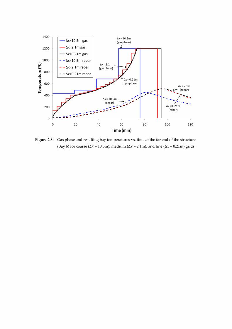
Figure 2.8: Gas phase and resulting bay temperatures vs. time at the far end of the structure

(Bay 6) for coarse (∆𝑥 = 10.5m), medium (∆𝑥 = 2.1m), and fine (∆𝑥 = 0.21m) grids.

0

200

400

600

800

1000

1200

1400

0 20 40 60 80 100 120

Tem

pera

ture

(o C)

Time (min)

Δx=10.5m gas

Δx=2.1m gas

Δx=0.21m gas

Δx=10.5m rebar

Δx=2.1m rebar

Δx=0.21m rebar

Δx = 2.1m(gas phase)

Δx = 10.5m(gas phase)

Δx = 0.21m(gas phase)

Δx = 10.5m(rebar)

Δx = 2.1m(rebar)

Δx =0. 21m(rebar)

(a)

(b)

Figure 2.9: (a) Gas phase and bay temperatures for rebar depths of 20, 30, 42 and 50mm;

(b) Peak bay temperature vs. fire area and rebar depth for ∆𝑥 = 0.21m.

0

200

400

600

800

1000

1200

1400

0 50 100 150 200 250

Tem

pera

ture

(o C)

Time (min)

Gas Phase at Bay 620mm Rebar30mm Rebar42mm Rebar50mm Rebar

Peak

Bay

Tem

pera

ture

(o C)

(a)

(b)

Figure 2.10: (a) Bay temperatures vs. time for each bay in the structure along its length; (b)

Variation of peak bay temperature with bay length for 5%, 10% and 25% fire

sizes.

0

100

200

300

400

500

600

0 50 100 150 200 250

Bay T

empe

ratu

re (o C

)

Time (min)

Bay 1

Bay 4 Bay 5 Bay 6

Bay 2Bay 3

400

440

480

520

560

600

0 5 10 15 20 25

Peak

Bay

Tem

pera

ture

(o C)

Bay Length (m)

5% Fire10% Fire25% Fire

Figure 2.11: Peak bay temperature vs. fuel load density for a range of heat release rates per

unit area.

350

400

450

500

550

600

650

700

750

0 200 400 600 800 1000 1200 1400 1600

Peak

Bay

Tem

pera

ture

(o C)

Fuel Load Density (MJ/m²)

200 kW/m²500 kW/m²800 kW/m²

Figure 2.12: Peak bay temperature vs. convective heat transfer coefficient for a range of

material emissivities and rebar depths.

400

500

600

700

800

900

0 20 40 60 80 100

Peak

Bay

Tem

pera

ture

(o C)

Convective Heat Transfer Coefficient (W/m²K)

ε=0.2, 42mm rebar

ε=0.5, 42mm rebar

ε=0.7, 42mm rebar

ε=1, 42mm rebar

ε=0.2, 20mm rebar

ε=0.5, 20mm rebar

ε=0.7, 20mm rebar

ε=1, 20mm rebar

Figure 2.13: Bay temperature vs. time for near field temperatures between 800 and 1200°C at

Bays 2 and 6.

0

100

200

300

400

500

600

0 50 100 150 200 250 300 350 400

Bay T

empe

ratu

re (o C

)

Time (min)

800°C Bay 6900°C Bay 61000°C Bay 61100°C Bay 61200°C Bay 6800°C Bay 2900°C Bay 21000°C Bay 21100°C Bay 21200°C Bay 2

Bay 2

Bay 6

Figure 2.14: Dimensions of the steel beam section analysed.

15mm

15mm

8mm

200mm

350mm

Not to scale

Figure 2.15: Peak steel temperature vs. fire size for unprotected, 60min rated, and 120min

rated steel beams at the far end of Bay 6 for a grid size of ∆𝑥 = 0.21m.

0

200

400

600

800

1000

1200

1400

0% 10% 20% 30% 40% 50% 60% 70% 80% 90% 100%

Stee

l Tem

pera

ture

(o C)

Fire Area

Unprotected60min120min

Figure 2.16: Temperature vs. time for the gas phase plus all three steel beam types at the

midpoint of Bay 2 and the far end of Bay 6.

0

200

400

600

800

1000

1200

1400

0 50 100 150 200 250 300

Tem

pera

ture

(o C)

Time (min)

Bay 6, GasBay 2, GasBay 6, Unprotected SteelBay 2, Unprotected SteelBay 6, 60min SteelBay 2, 60min SteelBay 6, 120min SteelBay 2, 120min Steel

Midpoint of Bay 2

End of Bay 6

Figure 2.17: Comparison of bay temperatures calculated using the base case, the standard

fire, and two Eurocode parametric temperature-time curves.

0

100

200

300

400

500

600

700

800

0 50 100 150 200 250

Bay T

empe

ratu

re (o C

)

Time (min)

Base CaseEC - 25% VentilationEC - 100% VentilationStandard Fire

Base Case equivalent to 106 min Standard Fire

106 min

(a)

(b)

Figure 2.18: Relative change in bay temperature vs. percentage change in each (a) building

parameter and; (b) physical or numerical parameter.

-35%

-25%

-15%

-5%

5%

15%

25%

35%

45%

-100% -50% 0% 50% 100% 150% 200% 250% 300%

Rela

tive

Bay T

empe

ratu

re C

hang

e

Percentage Change from Base Case Value

Fire Size

Rebar Depth

Fuel Load

Bay Size

-35%

-25%

-15%

-5%

5%

15%

25%

35%

45%

-100% -50% 0% 50% 100% 150% 200% 250% 300%

Rela

tive

Bay T

empe

ratu

re C

hang

e

Percentage Change from Base Case Value

Fire Size

Grid Size

Emissivity

Conv HT Coeff

Tnf (Concrete)