Transportation Data Research Laboratory: Data … · Transportation Data Research Laboratory: Data...
87
Transportation Data Research Laboratory: Data Acquisition and Archiving of Large Scaled Transportation Data, Analysis Tool Developments, and On-Line Data Support Final Report Prepared By: Taek M. Kwon Transportation Data Research Laboratory Northland Advanced Transportation Systems Research Laboratories (NATSRL) University of Minnesota Duluth 2006 (Revised 2008) Published by: Center for Transportation Studies, University of Minnesota 200 Transportation and Safety Building 511 Washington Ave SE Minneapolis, Minnesota 55455 The contents of this report reflect the views of the authors, who are responsible for the facts and the accuracy of the information presented herein. This document is disseminated under the sponsorship of the Department of Transportation University Transportation Centers Program, in the interest of information exchange. The U.S. Government assumes no liability for the contents or use thereof. This report does not necessarily reflect the official views or policy of the Northland Advanced Transportation Systems Research Laboratories, the Intelligent Transportation Systems Institute or the University of Minnesota. The authors, the Northland Advanced Transportation Systems Research Laboratories, the Intelligent Transportation Systems Institute, the University of Minnesota and the U.S. Government do not endorse products or manufacturers. Trade or manufacturers' names appear herein solely because they are considered essential to this report.
Transcript of Transportation Data Research Laboratory: Data … · Transportation Data Research Laboratory: Data...

Transportation Data Research Laboratory: Data Acquisition and Archiving of Large Scaled
Transportation Data, Analysis Tool Developments, and On-Line Data Support
Final Report
Prepared By: Taek M. Kwon
Transportation Data Research Laboratory Northland Advanced Transportation Systems Research Laboratories (NATSRL)
University of Minnesota Duluth
2006 (Revised 2008)
Published by: Center for Transportation Studies, University of Minnesota
200 Transportation and Safety Building 511 Washington Ave SE
Minneapolis, Minnesota 55455 The contents of this report reflect the views of the authors, who are responsible for the facts and the accuracy of the information presented herein. This document is disseminated under the sponsorship of the Department of Transportation University Transportation Centers Program, in the interest of information exchange. The U.S. Government assumes no liability for the contents or use thereof. This report does not necessarily reflect the official views or policy of the Northland Advanced Transportation Systems Research Laboratories, the Intelligent Transportation Systems Institute or the University of Minnesota. The authors, the Northland Advanced Transportation Systems Research Laboratories, the Intelligent Transportation Systems Institute, the University of Minnesota and the U.S. Government do not endorse products or manufacturers. Trade or manufacturers' names appear herein solely because they are considered essential to this report.

Executive Summary
The Transportation Data Research Laboratory (TDRL) at the University of Minnesota Duluth developed a Data Center (DC) in 2003 and completed online automation for two large sets of Minnesota Department of Transportation’s (Mn/DOT’s) Intelligent Transportation Systems (ITS) data in 2004. The two data sets are the Regional Transportation Management Center (RTMC) traffic data and the statewide Road Weather Information System (RWIS) data. For archiving, a new data archiving format, referred to as the Unified Transportation Sensor Data Format (UTSDF), was developed. This format allows archiving of many types of transportation sensor data using a single format, regardless of the sensor types. Presently, the TDRL DC automatically acquires the RWIS and traffic data from the Mn/DOT, archives them, and posts the data on the web for online distribution.
With the availability of archived ITS data, TDRL performed several research projects which are developed from Mn/DOT problem statements. Mn/DOT’s office of Transportation Data and Analysis (Mn/DOT TDA is responsible for providing Automatic Traffic Recorder (ATR) (also called continuous count) and short count data for the entire state. Since the TDRL DC houses the loop data for the entire Twin Cities’ freeway network, TDA requested TDRL to generate the ATR and short duration count data from the archived loop data. This request was formed as a project and successfully completed (Kwon, 2004). An on-line automation process was integrated to automatically generate the data and remotely provide the data service. During this project, data imputation algorithms were developed as a part of the project to estimate missing data. These algorithms and experimental results are included as a part of this report.
Utilizing the archived traffic data, the TDRL also developed a method of detecting faulty loops using loop volume and occupancy data. With nearly 5,000 loop detectors in the Twin Cities’ freeway network, it is difficult to manually test and repair the faulty detectors. The algorithm developed classifies detectors into four classes: healthy, marginal, suspicious, and highly suspicious detectors. Among them, the suspicious and highly suspicious detectors are the targets of maintenance. This software was tested and evaluated by the Mn/DOT RTMC maintenance engineers. The algorithm and experimental results are included as a part of this report.
Another project was created to explore opportunities in cross-utilization of RWIS and traffic data. Weather and road surface conditions are rarely incorporated into traffic models, such as in travel time prediction. Many aspects of weather impact on traffic are still unknown, and this study focuses on several of them, utilizing the archives of the statewide RWIS and traffic data at TDRL. The first one is to find out which RWIS parameter correlates most to traffic. This can be studied by constructing a correlation coefficient matrix, consisting of all possible combinations of RWIS and traffic parameters. Next question explored is the impact of different pavement conditions on daily traffic volume. Its answer provides information on how much the trip demands are influenced by weather and pavement conditions. Another interesting question studied is how the peak hour traffic volume is affected by weather conditions. This question addresses whether motorists try to avoid driving during peak hours when weather conditions are poor. Another aspect explored is whether the accuracy of travel time prediction can be increased by incorporating pavement conditions on to the prediction model. The details of this project are presented.
Another task completed by the TDRL is the development of a diagnostic tool referred to as a WIM Probe for the state’s Weigh-In-Motion (WIM) systems. Current WIM systems expose neither the raw WIM signals nor the weight computation processes to users, making it difficult to

identify faulty conditions of WIM systems. The WIM Probe was developed to provide the diagnostic needs of the current WIM systems. It provides analysis on faulty signals and computational errors, which can be used for system maintenance. The results of this project are included as a part of this report.

Table of Contents
CHAPTER 1: Introduction................................................................................................ 1
CHAPTER 2: Unified Transportation Sensor Data Format (UTSDF)........................... 4 2.1 Archiving Needs of ITS-Generated Data .......................................................................... 4 2.2 Assumption on Transportation Sensor Data (TSD)......................................................... 5 2.3 Basic UTSDF Archive File.................................................................................................. 5 2.4 Daylets .................................................................................................................................. 7 2.5 Log and Missing Information ............................................................................................ 8 2.6 Data Compression ............................................................................................................... 9 2.7 Organization of Archive Directories ............................................................................... 10 2.8 More Complex Structure of UTSDF: Monthlets and Yearlets....................................... 11 2.9 Binary UTSDF................................................................................................................... 12 2.10 Example Fields of Daylets .............................................................................................. 12 2.11 Concluding Remarks ...................................................................................................... 15
CHAPTER 3: Treatment of Missing Data Using Imputation........................................ 16 3.1 Introduction on Missing Data .......................................................................................... 16 3.2 Classification of Missing Data Patterns .......................................................................... 17
3.2.1 Spatial and Temporal Characteristics of Traffic Data................................................................ 17 3.2.2 Classification by a Tree Structure of Missing Data Patterns...................................................... 17
3.3 Multiple Imputation Algorithms ..................................................................................... 20 3.3.1 Basic Concept ............................................................................................................................ 20 3.3.2 TDRL Algorithms...................................................................................................................... 21
3.4 Implementation ................................................................................................................. 26 3.4.1 Detection of Missing and Incorrect Volume Counts.................................................................. 26 3.4.2 Implementation of Imputation.................................................................................................... 26
3.5 Concluding Remarks and Future Work ......................................................................... 29 CHAPTER 4: Detector Fault Identification Using Freeway Loop Data....................... 30
4.1 Introduction....................................................................................................................... 30 4.2 Classification...................................................................................................................... 31 4.3 Measurement Parameters ................................................................................................ 33 4.4 Algorithm Description ...................................................................................................... 35 4.5 Test Using Mn/DOT Loop Repair Record...................................................................... 38 4.6 Conclusion.......................................................................................................................... 39
CHAPTER 5: Weather Impact on Traffic ...................................................................... 40 5.1 Introduction....................................................................................................................... 40

5.2 Site Selection and Data Source......................................................................................... 40 5.3 Basic Methodologies Used to Analyze Weather Impact on Traffic .............................. 41
5.3.1 Correlation coefficients.............................................................................................................. 41 5.3.2 Effect of pavement conditions on daily total volume................................................................. 42 5.3.3 Effect of pavement conditions on traffic dynamics.................................................................... 42
5.4 Methodology to Analyze Impact on Travel Time Prediction........................................ 43 5.4.1 Travel time estimation ............................................................................................................... 43 5.4.2 Time-varying coefficients for travel time prediction ................................................................. 43
5.5 Experimental Results ........................................................................................................ 45 5.5.1 Correlation Coefficient Matrix................................................................................................... 45 5.5.2 Impact of Pavement Conditions on Daily Traffic Volume ....................................................... 47 5.5.3 Impact of pavement conditions on congestion ........................................................................... 49 5.5.4 Impact of inclement weather conditions on travel time prediction ............................................ 55
5.6 Chapter Conclusion .......................................................................................................... 65 CHAPTER 6: Weigh-In-Motion Probe........................................................................... 66
6.1 Introduction....................................................................................................................... 66 6.2 Hardware Setup ................................................................................................................ 66 6.3 Data Acquisition................................................................................................................ 67 6.4 Data Analysis ..................................................................................................................... 69
6.4.1 Data navigation .......................................................................................................................... 69 6.4.2 Axle signal analysis and weight computation ............................................................................ 70 6.4.3 Weight Calibration..................................................................................................................... 72
6.5 Static Weight Test Tool .................................................................................................... 73 6.6 Signal Anomalies and Treatments................................................................................... 74 6.7 WIM Probe Technical Information................................................................................. 76 6.8 Concluding Remarks ........................................................................................................ 76
References ........................................................................................................................ 77

List of Tables TABLE 2-1: RWIS DAYLET FILE EXTENSION FIELDS AND PARAMETERS ...................................................... 13 TABLE 2-2: PRECIPITATION INTENSITY ......................................................................................................... 14 TABLE 2-3: PRECIPITATION TYPE.................................................................................................................. 14 TABLE 2-4: SURFACE CONDITIONS................................................................................................................ 15 TABLE 4-1: TERMINOLOGY FOR LOOP REPAIR RECORDS IN MN/DOT RTMC .............................................. 32 TABLE 4-2: ALGORITHM DETECTION RESULTS ............................................................................................. 39 TABLE 5-1: RWIS SITES AND DETECTORS IN THE PROXIMITY ...................................................................... 41 TABLE 5-2: CORRELATION COEFFICIENT MATRIX FOR JANUARY 2005 AT LITTLE CANADA SITE ................. 46 TABLE 5-3: CORRELATION COEFFICIENT MATRIX FOR JUNE 2005 AT THE LITTLE CANADA SITE ................. 46 TABLE 5-4: SURFACE CONDITIONS IN NUMBER OF HOURS AND TRAFFIC VOLUME AT THE LITTLE CANADA
SITE IN JANUARY 2005 ........................................................................................................................ 48 TABLE 6-1: OUTPUT FILES AND DATA FORMAT ............................................................................................ 71 TABLE 6-2: WIM PARAMETER COLUMNS ..................................................................................................... 72
List of Figures FIGURE 2.2: DAYLETS COMPRESSED IN A UTSDF ARCHIVE FILE..................................................................... 9 FIGURE 3.1: TYPICAL ANNUAL MISSING PERCENTAGES OF A STATION (STATION NUMBER 1078E) ................ 18 FIGURE 3.2: CLASSIFICATION OF MISSING PATTERNS IN A TREE STRUCTURE ................................................. 19 FIGURE 3.3: EFFECT OF NBLR: BEFORE IMPUTATION (TOP) AND AFTER IMPUTATION (BOTTOM) ................. 23 FIGURE 3.4: EFFECT OF BLOCK IMPUTATION BY ALGORITHM 3: THE TOP GRAPH SHOWS BEFORE BLOCK
IMPUTATION AND THE BOTTOM GRAPH SHOWS AFTER BLOCK IMPUTATION. ........................................ 25 FIGURE 3.5: BLOCK DIAGRAM OF IMPUTATION STEPS IMPLEMENTED........................................................... 28 FIGURE 4.1: DECISION TREE FOR LOOP-DETECTOR DIAGNOSTICS AND CLASSIFICATION, PART 1 ................... 36 FIGURE 4.2: DECISION TREE FOR LOOP-DETECTOR DIAGNOSTICS AND CLASSIFICATION, PART 2. .................. 37 FIGURE 5.1: LOCATION OF RWIS SITES IN AND AROUND THE METRO AREA USED FOR THE STUDY................ 40 FIGURE 5.2: EFFECT OF PAVEMENT CONDITIONS ON THE TRAFFIC VOLUME OF LITTLE CANADA. THE
VOLUME/OCCUPANCY GRAPHS OF THE CORRESPONDING DAYS ARE SHOWN BELOW EACH LINE GRAPH.50 FIGURE 5.3: EFFECT OF SEVERE SNOW CONDITIONS ON THE TRAFFIC VOLUME. THE VOLUME/OCCUPANCY
GRAPHS OF THE CORRESPONDING DAYS ARE SHOWN BELOW EACH LINE GRAPH. ................................. 51 FIGURE 5.4: EFFECT OF DAMP PAVEMENT CONDITIONS ON TRAFFIC. ............................................................. 52 FIGURE 5.5: EFFECT OF WET PAVEMENT CONDITIONS ON TRAFFIC. ............................................................... 53 FIGURE 5.6: EFFECT OF DIFFERENT PAVEMENT CONDITIONS ON THE TRAFFIC VOLUME. THE
VOLUME/OCCUPANCY GRAPHS OF THE CORRESPONDING DAYS ARE ALSO PRESENTED. ........................ 54 FIGURE 5.7: TRAFFIC IS AFFECTED BY SEVERE SNOW CONDITIONS THAT REDUCE THE VOLUME AND AVOID
CONGESTION AND HENCE FACILITATES FREE FLOW CONDITIONS. THE PERCENTAGE PREDICTION ERROR OF TRAVEL TIME IS ALSO NEGLIGIBLE. ................................................................................................. 56
FIGURE 5.8: TRAVEL TIME PREDICTION IS AFFECTED BY THE SNOW CONDITIONS WHICH CAUSE CONGESTION. THE PPE GRAPH SHOWS THE ERROR THAT OCCURS DUE TO THE CHANGE IN WEATHER........................ 58
FIGURE 5.9: TRAVEL TIME WAS AFFECTED BY DAMP CONDITIONS. THE DAMP CONDITIONS INCREASED THE TRAVEL TIME, AND THE TV PREDICTION MODEL UNDERESTIMATES THE TRAVEL TIME. THE TVWI MODEL CORRECTS THE DIFFERENCE AND IMPROVES THE PREDICTION ACCURACY. .............................. 60
FIGURE 5.10: TRAVEL TIME IS AFFECTED BY SNOW CONDITIONS FOR THE WHOLE DAY. THE SNOW CONDITIONS INCREASE THE TRAVEL TIME AND THE PREDICTION TENDS TO UNDERESTIMATE THE TRAVEL TIME. ...................................................................................................................................... 62
FIGURE 5.11: THE TV TRAVEL TIME PREDICTION IS AFFECTED BY CHANGING WEATHER CONDITIONS AND IS UNABLE TO PREDICT THE TRAVEL TIME ACCURATELY. THE TVWI MODEL REDUCES THE ERROR BY INCORPORATING THE WEATHER CONDITIONS. ...................................................................................... 64
FIGURE 6.1: WIM PROBE HARDWARE SETUP ................................................................................................ 66

FIGURE 6.3: WIMDAQLT.EXE INITIAL SCREEN............................................................................................. 68 FIGURE 6.4: DATA ANALYSIS SCREEN .......................................................................................................... 70 FIGURE 6.5: COMPLETED DATA WINDOW ...................................................................................................... 72 FIGURE 6.6: STATIC WEIGHT TESTING TOOL .................................................................................................. 73 FIGURE 6.7: FACTORY SENSITIVITY SETTING SPECIFIED ON THE SENSOR ....................................................... 74 FIGURE 6.8: WIM SIGNAL WITH PIEZOELECTRIC RECOVERY PROBLEM ......................................................... 75 FIGURE 6.9: A SEVERE CASE OF PIEZOELECTRIC RECOVERY PROBLEM. ......................................................... 75 FIGURE 6.10: LINE NOISE .............................................................................................................................. 75

1
CHAPTER 1: INTRODUCTION
One of the key features of today’s Intelligent Transportation Systems (ITS) has been utilization of a variety of traffic and road weather sensors to improve the overall transportation system performance. ITS-generated data has been successfully used in managing operations or monitoring transportation system conditions (ASUS, 2000; Magiotta, 1998). Recently, increasing deployments of ITS brought an awareness that ITS-generated data offers a great promise beyond the present operational and monitoring uses, e.g., they can be used for planning and research (ASUS, 2000). Unfortunately, much of today’s ITS generated data has not been archived, i.e. much of the historical sensor data has been continuously lost. Recognizing these problems, the U.S. Department of Transportation (DOT) created a subcommittee called the Archived Data User Service (ADUS) as an official program for studying transportation data archiving as a part of the National ITS Architecture (NCHRP Report 446, ADUS, 2000). ADUS defines the archiving problem as “urgent” and promotes data archiving. The Transportation Data Research Laboratory (TDRL) as a part of Northland Transportation Systems Research Laboratories (NATSRL) at the University of Minnesota Duluth (UMD) was established to fill in Minnesota’s archiving needs by archiving the State’s ITS generated transportation data.
There are several challenges in archiving large scaled ITS generated data. A few of them are briefly discussed. (1) Increasing deployment of ITS by State DOTs have created the data size to an unprecedented amount, introducing a technical barrier that has worked against archiving the statewide data. Technologies related to reliable, large storages and efficient retrieval system became nontrivial. (2) Data must continuously flow to a central location for archiving from the various locations in the state without interruption of communication or device failures. Within the statewide network, many failure points that are hard to manage exist, and thus reliable aggregation of statewide data is a continuous challenge. (3) No standard archive formats or tools are available for archiving statewide data. With these challenges, archiving in State DOTs has been performed in partial with non-uniform formats, which often defeats the main purpose, i.e., sharing the data. Archiving and managing statewide data is expensive, complex, and nontrivial due to the challenges described above, and many reports concur with this opinion (Edwards, 1995; Fairhead, 1995; Fogarty, 1994). As an alternative approach, Kodor states that there is no such thing as a complete data warehouse, either in terms of the environment or the tools (Kador, 1995). In other words, a large scale data center or warehouse cannot be built as a one-time complete system, but it should be an evolving concept.
The TDRL’s objective shares the general data warehousing view, but the implementation approach deviates from the common approach. In most data warehouse implementations, the high cost and complexity is largely contributed to the reliance on the structure of traditional Relational Database Management Systems (RDBMS). RDBMS can manage all different types of data formats but at a cost of complex data tables and expanded data size. As an example, a RDBMS-based traditional approach has been pursued by the researchers at the University of California Berkeley through a PATH research program (Chen, 2001) and also by the University of Virginia (Smith, 2003) using traffic data. These trials have shown that they are expensive (several million dollars) and complex. At TDRL, we set a goal of archiving the Minnesota Department of Transportation’s (Mn/DOT) ITS generated for the next 100 years (or more) by strictly establishing and following the standard data formats but without using RDBMS. This rigid approach takes more time initially, but it is expected to be more economical and provides more efficient retrievals for large scaled data.
As TDRL started working with ITS-generated data and accumulated experiences on the characteristics of data, it learned that most ITS generated data can be expressed into a uniform format. TDRL studied Common Data Format (CDF) developed by the National Space Science

2
Data Center (NSSDC) (Goucher, 1994) and Hierarchical Data Format (HDF, 1990) developed by the National Center for Supercomputer Applications (NCSA), as well as RDBMS as an initial study to find a solution (Kwon, 2003). During the fiscal year 2003/2004, TDRL finally developed a new framework referred to as the Unified Transportation Sensor Data Format (UTSDF) for archiving large-scale transportation data and decided to archive all future data using UTSDF (Kwon, 2004). UTSDF creates an archive that is compact and easy to retrieve, and provides a uniform standard for archiving. The result is that the users of TDRL archives only need to learn a single format to use the entire data, which promotes sharing of the data. The properties of UTSDF are summarized:
Unified data format for all types of transportation sensor generated data Adaptable for changes in spatial configuration of sensors Easy to create the archive and retrieve the data Simple to learn and manage Fast retrieval of large amount of data Compatible with all types of computers and operating systems Compact size for efficient storage and distribution Inclusion of meta data (description of data) Low cost to build and manage large scale data
The efficiency of UTSDF can be demonstrated using the archive size and its retrieval
performance (Kwon, 2004). When a single day amount of RTMC traffic data was stored into a RDBMS (MS SQL), the size became 370MB. When the same data was archived using UTSDF, its size shrank to 12MB. This means that UTSDF achieves with a storage efficiency of 3,000% over RDBMS. For the statewide Road Weather Information System (RWIS) data, the size of raw data for a single day is about 4.1MB. When the same data was archived using UTSDF, its size shrank to 415KB, which is a 10:1 storage efficiency (Kwon, 2004). Such storage efficiency is extremely important when the size of the raw data is very large. Retrieval efficiency of the archive was also tested against RDBMS. The benchmark test showed that UTSDF retrieval time of large amount of data (larger than 370MB) was about 80 times faster than that of RDBMS. With these initial study results, TDRL concluded to adopt UTSDF as the TDRL’s archiving standard.
With the completion of the development of UTSDF, the methodology for archiving Minnesota’s statewide ITS-generated data is now well established. Presently, RTMS traffic and statewide RWIS data are daily archived. Also, a data center that houses several servers and large network storages (two terabytes) was established at the UMD campus.
This report describes the research works completed during the fiscal years (FY) 2003/2004 and 2004/2005 at TDRL, supported by the NATSRL program. This includes development of UTSDF and other data related works. Although a significant part of the fund was used to build a data center and hiring students for working on the archiving, only the research components are described in this report. This report is organized in six chapters. Excluding Chapter 1: Introduction, the rest of the chapters described individual projects. Chapter 2 describes details of UTSDF format. Chapter 3 describes imputation algorithms that restore missing values from a data set. These imputation techniques were developed for the short count and continuous count data that are supplied to the Mn/DOT office of Transportation Data & Analysis (TDA), which is one of the data services at TDRL. Since data imputation is important for improving data quality, the chapter focuses on the algorithm developments and experimental results. Chapter 4 describes a detector fault identification technique, developed using freeway loop data. With nearly 5,000 loop detectors in the Twin Cities’ freeway network, it is difficult to manually test and repair the faulty detectors. Therefore, a software approach was developed. This software tool analyzes a large set of loop data and summarizes what types of maintenance checks and repairs

3
are needed for each loop. This project is described by focusing on the identification algorithm and the classification scheme.
Chapter 5 describes the study results of weather impacts on traffic. With the availability of RWIS and traffic data at TDRL, this project analyzed correlation between weather and traffic parameters, impact on traffic demand, impact on congestion, and impact on travel time. Chapter 6 describes the development of a Weigh-In-Motion (WIM) Probe. Today’s WIM systems expose neither the raw WIM signals nor the computation processes. Consequently, when results from a WIM system are questionable, no easy way of identifying the problem source exists. In FY 2003/2004, Mn/DOT TDA requested TDRL to develop a diagnostic tool for the current Mn/DOT WIM systems. The result is the development of a diagnostic tool called the WIM Probe. It was designed as a portable system that provides analysis on faulty signals and computational errors.

4
CHAPTER 2: UNIFIED TRANSPORTATION SENSOR DATA FORMAT (UTSDF) 2.1 Archiving Needs of ITS-Generated Data
Today’s transportation systems utilize a wide range of sensors to monitor, control, and analyze many parts of transportation systems. The sensor usages have been further accelerated by the US DOT’s emphasis on ITS in recent years. While the usage of sensors has increased, archiving (or saving) of the sensor data has not (ADUS, 2000). In most transportation departments, only a small fraction of sensor data has been archived. For example, each intersection typically includes a number of vehicle detecting sensors to optimize the timing of the traffic controller, but the data is rarely archived.
There are a number of reasons that archiving of Transportation Sensor Data (TSD) has not been eagerly pursued by transportation departments. First, the most influential factor is the cost, i.e., while the cost of sensors is low, the cost of archiving its data is expensive. Consequently, archiving has been frequently unwelcome by maintenance engineers and managers. Second, continuous flow of data from transportation sensors adds an additional burden to the management of data and archiving. Sensors continuously operate and generate data once they are activated, and the amount of data can be quickly accumulated to a large amount. Moreover, all parts of the data acquisition system must continuously operate without disruption. For maintenance personnel, archiving is additional work and a burden because missing or lost data can be a responsibility. In addition, archiving often reveals the weakness or reliability of the system, which sometimes is unpleasant. Third, when data is collected from many different types of sensors, which would be the case in Road Weather Information Systems (RWIS), management of data is complicated. To date, there exists no uniform and efficient data format that can be used for archiving all types of sensor data. As a result, management of data from various acquisition systems developed by many different manufacturers is in itself a challenge. For example, a large amount of work is required just to keep up with the data format differences and modifications, incompatible file formats, version changes of software tools and operating systems, etc. Therefore, acquisition, archiving, and maintenance of data for a large network of sensors in today’s ITS are not trivial.
The next question is then “Why do we need archiving?” or “Do we really need to archive sensor data?” The answer would depend on the needs. However, if we assume that system analysis (performance, reliability, etc.) is needed at some point in the future, archiving of data would be required since analyzing a system without historical data is unreliable. Therefore, the more important question on archiving is not in the need of or not, but in what extent, i.e., which selected locations, what sensors, and how long the data should be archived. The UTSDF introduced in this chapter is an attempt towards making TSD collection and archiving simple, regardless of the number of sensors, sensor types, and variability such as location changes or removals.
An important step in developing a large scale TSD archives is to create a uniform and efficient data format that is simple and independent of operating systems and programming languages. If a unified format is developed, users only need to learn a single type of data format for archiving and use of the archived data, which would in turn encourage archiving.
At the TDRL, the need for the development of UTSDF was born out of the needs in developing statewide archives of TSD that have characteristics of large scaled data and variety of data types, including non-numeric data. In developing UTSDF, the followings objectives were set.

5
A single unified data format for all types of transportation sensors Simple to understand and use Easy to manage Compatible with all types of computers, OS’s, and programming languages Easy to distribute or share large amount of data Compact, compressed form No or low cost in adopting the technology Fast and easy retrieval of a large amount of data from the archived data Adaptable for changes in sensor locations or configuration Inclusion of description of data (meta data)
This chapter describes the format of UTSDF and archiving methodologies that could be readily applied for statewide TSD archives.
2.2 Assumption on Transportation Sensor Data (TSD)
We refer all types of sensors (electrical, magnetic, mechanical, optical, chemical, etc) that are used in transportation systems as transportation sensors. Transportation sensors are typically used in monitoring the state or condition of a transportation system component and often placed under the pavement or near the roadways. The digitized values or decision results of the sensor state comprise the sensor data. One of the assumptions that can be made for TSD is that most sensor readings are obtained at a fixed interval (i.e., sampling rate). For example, if traffic counting data is collected for every 30-second interval, there will be 2,880 data points per day. The sampling rate is commonly determined based on the sampling theorem, i.e. twice the bandwidth (also called a Nyquist rate) of the original signal (Alan, 1893). If sensor readings are recorded at a Nyquist rate, the sampling theorem guarantees that the complete original signal can be reconstructed from the sampled data (Alan, 1893). Consequently, it is assumed that re-sampling is possible from the reconstructed signal without loss of information.
Some sensors do not produce numerical values but descriptive conditions. For example, pavement sensors produce pavement conditions such as wet, dry, ice, etc. As long as those readings are recorded at a fixed rate, the UTSDF should be able to store the data. Another consideration is that a single sensor may produce multiple types of values. For example, a single inductive loop detector produces two types of data, volume and occupancy. In order to differentiate between the sensor and values produced, each type of sensor values is referred as a parameter, i.e., volume and occupancy are parameters of inductive loop detectors. These parameters are the final data (or variables) that are stored in a UTSDF archive.
2.3 Basic UTSDF Archive File
A single UTSDF archive file (or simply UTSDF file) is a zip-compressed file of many small data files called daylets (described in the Section 2.4). A single UTSDF file is created based on the time unit of a single day, in which it is a collection of daylets from the same day. The file name is given using the format:
yyyymmdd.Class_Name
where the date of the archived data is encoded as the file name with eight digits, i.e., yyyy is the year, mm is the month, and dd is the day. The Class_Name is the name of the sensor class such as

6
RWIS, traffic, or WIM (Weigh-in-Motion). For example, an RWIS archive file on Feb 23, 2003 would have the name 20030223.rwis. Similarly, the traffic file on the same day would have the name 20030223.traffic. As a result, when the archived files are viewed as a sorted list, it should be in a chronological order. Different classes of the archived files are stored in separate directories, and thus one year of complete RWIS or traffic archive would consist of 365 UTSDF files. The structure of a single UTSDF file is illustrated as a block diagram in Figure 2.1. The size of a daylet would depend on the type of parameters it stores.
Daylet 1
Daylet 2
Daylet 3
Daylet n
Figure 2.1: A UTSDF file consists of n daylets. The number of daylets in an archive file would depend on the different types of parameters and the number of sensor locations.

7
2.4 Daylets
Daylets are the basic components of a UTSDF file, and each contains the actual sensor data. The name of each daylet is assigned based on the spatial information (i.e., location) and the parameter type of the sensor, while the name of UTSDF file is assigned using the temporal information (date) and the sensor class name. This name convention utilizes the temporal and spatial properties of TSD, which are discussed in (Kwon, 2004). The basic name format consists of four fields separated by dots and is shown below:
SysID.SiteID.SensorID.ParaName
SysID: System ID. It is a unique number assigned for system characteristics such as the sensor type differentiated by different manufacturers.
SiteID: Site ID. It is a unique number assigned to each site based on the geographical location of the sensor.
SensorID: Sensor ID. It is a unique number assigned for multiple sensors of identical types within a site (same location). For example, if three pavement temperature sensors are installed at a site, the sensors are assigned with SensorID, 0, 1, and 2.
ParaName: Parameter Name. It is a shortened parameter name without any space. For example, air temperature is shortened as “atemp” in this field.
UTSDF itself does not strictly define each field. The four-field name convention is
provided as a recommendation. It is the archive provider’s responsibility that each field is defined, documented, and provided along with the data. An example documentation of these definitions are provided in Section 2.11, which are the actual UTSDF archives of the Mn/DOT RWIS data at TDRL.
For illustration, the name convention of daylets for statewide RWIS used in Mn/DOT data is used. Assume that we need to create a daylet for air temperature for System ID=330, Site ID=17, and Sensor ID=0, then the daylet’s name would be assigned as “330.17.0.atemp”.
If the statewide system consists of only one type of system and no duplicated sensors in each site, the first three fields can be combined as a single field of site ID numbers, but this will limit the flexibility and future extensibility. At a minimum two fields must exist, i.e. the Site ID and the ParaName to be qualified as a UTSDF.
The content of a daylet is a long string of ASCII characters that represent data of a single day for the parameter it stores. Use of an ASCII string provides excellent portability and allows storage of both numeric and non-numeric data, although its file size is not minimized. Each datum within a daylet must have the same length (the same number of characters); so that the total string length of a daylet is always the datum length multiplied by the number of data items in the daylet. If a null datum exists, repetition of “N” characters for the allocated datum length is entered. Repetition of the same characters for null data is later efficiently compressed by the compression process. Since each datum has the same length, the daylet’s sampling period is precisely determined by dividing 24 hours by the number of data entries in the daylet, or vice versa. For example, if wind direction data is sampled at every 10 minutes and three digits are allocated for each datum to represent an angle in clockwise degree from north, the total string length of the wind-direction daylet would be 432 and it would contain 144 data entries. Time stamp is not entered for each datum since each datum is sampled at a fixed sampling rate within that day. We assume that data can be always reconstructed from the sampled data and re-sampled to produce the data for any time of the day based on the sampling theorem (Alan 1983). For the

8
negative numbers, a single character “ – “ is used as a prefix, but positive numbers do not use any prefix character. Example: Suppose that air temperature is sampled from a sensor for a single day with 10 minute intervals. The data collected from the sensor are degrees in Celsius and shown below:
00:00 27.5 00:10 10.5 00:20 5.8 00:30 N/A ; missing data 00:40 0.5 . . . 23:40 -13.5 23:50 -10.5 23:50 -5.5 Suppose that four digits are allocated for each datum representing a unit of one-tenth
degrees in Celsius. Then, the string for the above data is packed as a single ASCII string by simply concatenating four digit numbers in a chronological order, i.e.
When this string is saved as a file with the predefined daylet name fields, it becomes a daylet for the air temperature for the given date of the UTSDF file. In the daylet ASCII string, it is important to note that no line breaks, commas, or spaces are used to separate the data. Such data separators are not needed, since the same number of ASCII characters for each datum is used within each daylet. One may be concerned about the increased size of the data due to the use of ASCII string and fixed length. However, since the daylets are later compressed in an archive file, the size of the initial data is significantly reduced. According to previous study, the compression algorithm efficiently shrank the ASCII strings with fixed data length. The size was often smaller than the zip-compressed results of the equivalent size of binary data (Kwon, 2004).
One advantage of using daylets in archiving is that since daylets are independent of each other in terms of the storage, they can be easily added or removed without any modification in the overall data structure. For example, as more sensors are installed at new locations or removed from old locations, daylets can be freely added or removed in the archive. This independence of daylets makes the overall management of the archive flexible and simple.
2.5 Log and Missing Information
Each UTSDF archive file includes two special files. They are yyyymmdd.missing and yyyymmdd.log files where yyyymmdd is the numerical values of the year, month, and day of the archived date. The yyyymmdd.missing file includes a list of missing daylet names (null data for the entire day) on that day. The daylet list is separated by a comma.
The yyyymmdd.log file serves as meta data and includes information about the data in the archive file. The format of this file is not defined except that ASCII characters should be used. The archive provider should supply the documentation on the *.log file where meta data is stored. Any information the user of the archive must know, should be stored in this file, such as the number of active sites, the sites out of service, special events, etc.
027501050058NNNN0005…-135-100-055

9
2.6 Data Compression
A UTSDF archive file is simply a zip-compressed file of many daylets. When a single UTSDF file is uncompressed (unzipped), it should reproduce all of the original daylets that were compressed into a single archive file. Since most unzip tools allow unzipping of a single or just a few files, daylets can be selectively retrieved from a UTSDF file.
Zip compression uses a compression algorithm referred to as Deflate. Deflate combines the LZ77 algorithm (Ziv, 1977) for marking common sub-strings and Huffman coding (Huffman, 1952) to take an advantage of the different frequencies of occurrence of byte sequences in the file. Deflate does have an important advantage in that it is not patented (no need to obtain licenses). Thus, it is presently the most widely used file compression method. It is used in the WinZip™ freeware in Windows™ and the gzip program in Unix, and the jar files in Java. The Deflate algorithm is also a standard for the Internet Protocol payload compression (RFC 2394). Today, the term, zip or unzip, is commonly used, replacing the algorithm name Deflate. For programmers, free source codes are available from the Internet for zip and unzip. Also, many convenient commercial software tools, such as dynaZip, Sax.net, Xceed, ComponentOne, etc., are available for embedding unzip or zip functions into application programs. At TDRL, a freeware WinZip™ and DynaZip™ utilities have been used as the basic tool for compression and decompression. An example screen shot of compressed UTSDF file is shown in Figure 2.2. Notice that the average compression ratio is about 80%.
Figure 2.2: Daylets compressed in a UTSDF archive file.

10
2.7 Organization of Archive Directories A single UTSDF archive file contains the total data for a statewide sensor network for a
single day. UTSDF files are organized as a hierarchical format based on a file directory structure. File directory structure (or system) has been successfully used in storing all types of data since the beginning of the computer age and has proven very effective in handling large complicated data. There are a number of benefits in using a file system as the structure of archive organization. First, file system is such a familiar form to any computer users that it is probably the easiest structures to understand and manage. Second, it is one of the most stable and reliable parts of any computer operating system. Third, temporal, spatial, and computational hierarchies of TSD properties fit nicely into the hierarchical nature of the file directory structure (Kwon, 2004).
The organization of archives should be based on clarity and efficiency in retrieval of the data. Organization of two common TSD is considered, which are RWIS and traffic data. First, consider that we wish to build a statewide archive for traffic data. Since the number of traffic detectors used in a state is large, it is convenient to divide the data into districts to form a reasonable size of the archive files. Within each district, the sensors can then be given unique ID numbers or can be organized using dot separated fields as shown in Section 2.4. Each district directory is then further divided into year directories where daily UTSDF files are stored. This directory structure utilizes the division of data with familiarity, i.e., location and time. This structure is illustrated in Figure 2.3. In this case, if the district, year, date, and the detector ID number are known, the data can be quickly searched. Notice that spatial and temporal hierarchies of traffic data properties are alternatively utilized in the directory tree.
Next, consider a statewide RWIS archive. Since the number of RWIS stations in a state is typically less than 1,000 and the stations are centrally managed, dividing them into districts can result in small fragmented archived files. The presence of too many fragmented archived files leads to a lack of structural integrity. Therefore, it is more logical to organize the archive directories into year directories as shown in Figure 2.3. In this case, each UTSDF archive file would contain RWIS daylets for the entire state for a single day. TDRL presently uses this organization to archive the Mn/DOT’s statewide RWIS data. However, if the number of stations within a state were very large such as exceeding 5,000, then dividing the directories into districts would be more sensible. Again, the overall structure should utilize the temporal and spatial relations of the data since daylet’s names are organized based on spatial relations.
One important part of the UTSDF directory structure is the inclusion of /docs directories at the next to the root level as shown in Figure 2.3. In the /docs directory, the archive provider should include all documentations necessary to understand the archive. It helps the users of the archive, as well as for the maintenance of the archive. The documentation could include daylet field name definitions, string length allocated for each parameter, basic units, sensor locations, sensor manufacturer information, maintenance history, addition or removal of sensors, etc. Inclusion of the /docs directory follows the sprit of the inclusion of a log file inside the daily UTSDF file, i.e., description of the data is provided at multiple levels, directory level and daylet level.

11
2.8 More Complex Structure of UTSDF: Monthlets and Yearlets
Until now, archiving of raw sensor data was discussed for daily operation of archiving, where daylets are utilized. However, many applications frequently need to process a longer time span, such as statistical analysis of Average Annual Daily Traffic (AADT) or daily average/low/high temperatures of pavement. For those applications, expressing the data in a larger time span is necessary, such as a year rather than a single day. These needs can be met by introducing monthlets and yearlets, which are similar to daylets, except that they contain a whole month of data or a whole year of data.
Unlike daylets, monthlets and yearlets would require multiple parameters in a single file. For example, a yearlet storing daily average/low/high air temperatures for the entire year requires three parameters. In such a case, the yearlet should contain three long strings, one for the average, one for the low, and the remaining one for the high air temperatures. Each string contains 365 items and should follow the same principle used in daylets, i.e., fixed length for each datum. Each string should be separated by a pair of carriage return and line feed ASCII characters for distinction. Figure 2.5 illustrates a yearlet with three strings.
Traffic
District 1 District 2
District P
District i …
…
Year 1Year 2
Year M
Year i …
…
Day1.traffic Day2.traffic
DayN.traffic
… …
…
RWIS
Year 1Year 2
Year M
Year i …
…
Day1.rwiDay2.rwi
DayN.rwis
… …
…
docs
docs
Figure 2.3: Directory structure of statewide UTSDF archives: RWIS and traffic data example

12
In the reference (Kwon, 2004), a computational hierarchy was introduced, in which processed data is organized and archived as a hierarchical directory structure. In a very large system such as a statewide network of sensors, archiving of the processed data can be beneficial if they are frequently used or shared. Examples include AADT or daily average of RWIS parameters. For developing a directory structure for processed data, the structure of the examples given in Figure 2.3 is again recommended. More specifically, additional root directory can be created for the computational hierarchies for each class of data. In the above example, one directory can be created for processed RWIS data and another directory for processed traffic data. The child directories of the computational hierarchy would depend on the type of computation and data outcomes, which would essentially require development of a subdirectory structure for the specific needs. 2.9 Binary UTSDF
In a standard UTSDF, all of the sensor data in daylets, monthlets, and yearlets are stored using ASCII characters. However, if the data consists of only numerical values and fixed sizes, binaries could be used instead of ASCII characters. When the data in daylets are stored in binary, we refer the archive as binary UTSDF. In general, use of binary is not recommended, since they are less portable between different operating systems and programming languages. Moreover, binaries can create a compatibility problem of byte orders known as Little-Endian and Big-Endian, as well as the size definitions of integers and floating points. Since the benefits of data size in using binaries is diminished after zip-compression as demonstrated in (Kwon 2004), binary UTSDF is not recommended for archiving TSD.
2.10 Example Fields of Daylets This section provides example formats of daylet name fields and codes for RWIS which
are used at TDRL. Table 2-1 summarizes RWIS daylet file extensions and number of digits for atmospheric parameters, surface parameters, and sub-surface parameters. Table 2-2 summarizes numeric codes for precipitation intensity. Table 2-3 summarizes precipitation types. Table 2-4 summarizes pavement conditions.
String for daily average air temperature
Yearlet containing avg/low/high air temperature string
String for daily low air temperature
String for daily high air temperature
Figure 2.4: Yearlet example of daily avg/low/high temperature for the entire year.

13
Table 2-1: RWIS Daylet File Extension Fields and Parameters
Index Parameter File extension DigitsValues
Atmospheric Parameters 0 Air Temp atemp 4 Tenths of degree Celsius 1 Dew Temp dtemp 4 Tenths of degree Celsius 2 RH relhum 2 Percent, 100=PP 3 Wind Speed Avg. avgspd 4 Tenths of meters/sec 4 Wind Speed Gust gstspd 4 Tenths of meters/sec 5 Wind Direction Avg. avgdir 3 Clockwise degrees from North 6 Wind Direction Max. maxdir 3 Clockwise degrees from North 7 Precip Intensity pinten 1 See Table 1.1* 8 Precip Type ptype 1 See Table 1.2* 9 Visibility visib 5 Tenths of meter 10 Air Pressure apress 5 Tenths of millibar 11 Precip Rate prate 3 Tenths of Cm/hr. 12 Precip Accum paccum 4 Tenths Cm over 24 hr starting
at Midnight local time 13 10 min Solar 10msol 5 Tenths Joule/sq. meter 14 24 hr Solar 24hsol 6 Tenths Joule/sq. meter 15 24 hr Sun 24hsun 4 Minutes over 24hr 16 Air Temp Max amaxtemp 4 Tenths of degree Celsius 17 Air Temp Min amintemp 4 Tenths of degree Celsius 18 Wet Bulb Temp Wbtemp 4 Tenths of degree Celsius 19 Last Precip start Pstart 14 yyyymmddHHMMSS 20 Last Precip end Pend 14 yyyymmddHHMMSS 21 1 hr Precip Accum 1hpaccum 4 Tenths Cm 22 3 hr Precip Accum 3hpaccum 4 Tenths Cm 23 6 hr Precip Accum 6hpaccum 4 Tenths Cm 24 12 hr Precip Accum 12hpaccum 4 Tenths Cm 25 24 hr Precip Accum 24hpaccum 4 Tenths Cm Surface Parameters
0 Surface condition surcond 1 See Table 1.3* 1 Surface Temp surtemp 4 Tenths of degree Celsius 2 Freeze Temp frztemp 4 Tenths of degree Celsius 3 Chemical Pct. chmpct 2 Percent, 100=PP 4 Depth dpth 3 Hundredth of millimeter 5 Ice Pct. Icepct 2 Percent, 100=PP 6 Salinity Salin 5 Parts/100,000 7 Conductivity Conduc 4 Mhos
Sub-Surface Parameters 0 Surface Sensor Id surid 2 Integer 1 Subsurface temp subtemp 4 Tenths of degree Celsius 2 Subsurface moisture submoist 2 Percent 3 Delta-t delta 5 Picoseconds

14
Table 2-2: Precipitation Intensity
Classification Code None 0 Light 1 Slight 2 Moderate 3 Heavy 4 Other 5 Unknown 6 Anything else 7
Table 2-3: Precipitation Type
Classification Code None 0 Yes 1 Rain 2 Snow 3 Mixed 4 Light 5 Light Freezing 6 Freezing Rain 7 Sleet 8 Hail 9 Frozen A Unidentified B Unknown C Other D Anything else E

15
Table 2-4: Surface Conditions
2.11 Concluding Remarks UTSDF was developed for archiving a very large set of transportation sensor data that
includes many different types of sensors. Although its structure is simple, it can be used for developing well-organized, large archives. It is a TDRL’s hope that UTSDF is adopted in other state transportation departments so that ITS generated data can be easily archived and shared. Presently, Minnesota statewide RWIS and Twin Cities’ metro freeway traffic data have been fully archived using the UTSDF. In addition, TDRL is in the process of archiving the Minnesota statewide Weigh-in-Motion (WIM) and vehicle classification data.
The researchers at TDRL are continuously working on developing data visualization and analysis tools for UTSDF data. Some of public software tools have already been developed and distributed through the following web link.
http://www.d.umn.edu/~tkwon/TDRLSoftware/Download.html.
Classification Code Dry 0 Wet 1 Chemically Wet 2 Snow/Ice Watch 3 Snow/Ice Warning 4 Damp 5 Frost 6 Wet Above Freezing 7 Wet Below Freezing 8 Absorption 9 Absorption at Dewpoint A Dew B Black Ice Warning C Other Slush D
16
CHAPTER 3: TREATMENT OF MISSING DATA USING IMPUTATION
3.1 Introduction on Missing Data As in most real-world data, ITS generated data contains missing and incorrect data. Since
ITS traffic data is commonly collected 24 hours a day throughout the year using computerized data collection systems, presence of data loss due to hardware malfunctions at any site or along the transmission lines is highly probable. Construction, power outage, and temporary maintenance operations are unavoidable, which mostly likely lead to loss of data. For maintenance, missing data could provide invaluable information to diagnose the state of the sensor. However, for data reporting missing data can cause deviation in the statistical analysis.
Attempts to estimate missing data in a collection of ITS traffic data have been made with some success. Researchers at the Texas Transportation Institute (TTI) have explored regression analysis in combination of an Expectation-Maximization (EM) algorithm and compared the results with those from simple techniques such as straight-line interpolation and “factor-up” on traffic data (Gold, 2001). The results are very encouraging. The EM algorithm, however, is rather computationally intensive and, as the researchers conclude, the marginal improvement in performance did not weigh well against the time and effort that goes into the implementation of the EM algorithm. In this study, treatment of larger blocks of missing data was not addressed, which is a potential problem with EM. Schmoyer et al. (Schmoyer, 2001) proposed a simple filtering approach for detecting missing data and linear regression estimates for the treatment of missing data. Again, this approach does not address large blocks of missing data. A school of time series estimation and filtering approaches exists, which have been known to be effective in recovering missing data or removing noise from band-limited signals (Box , 1994; Chatfield, 1996; Naidu, 1996; Warner, 1998). Since most ITS generated data are obtained by sampling the state of a sensor at a constant rate such as 30 seconds or 5 minutes, they are indeed a time series and could be applied to the vast array of available time-series algorithms. However, no study results on time series restoration of ITS generated data are presently available to the best knowledge of the author.
Many rigorous research works on imputing missing data have been conducted in the field of statistics for applications in social science survey data, since such data most likely contains non-responses. Little & Rubin (Little, 1987) developed and laid foundations on the analysis of multiple imputation approaches on non-response survey data and suggested a number of statistical models based on historical inferences. These pioneering works are mostly based on likelihood estimates derived from formal statistical models. Schafer extended the analysis to incomplete multivariate datasets with continuous and discrete variables and applied EM algorithms and Monte-Carlo based Markov chain approaches. In a broad sense, the approaches mentioned can be called Bayesian approaches, because they explicitly use probability for quantifying uncertainty in inferences based on statistical data analysis (Gelman, 1995).
This chapter describes data imputation techniques developed for traffic data, as a part of TDRL research activities in FY 2004/2005.

17
3.2 Classification of Missing Data Patterns 3.2.1 Spatial and Temporal Characteristics of Traffic Data
Before investigating the missing traffic data patterns, it is important to recognize that
traffic data inherently holds spatial and temporal relationships if they are comprised of data from multiple detectors in multiple locations. Spatial relation refers to a geographical relation of detectors, and it may be characterized using the size of geographical area. For example, detectors could be characterized as detectors in a station, a road, a county, or a state. Similarly, temporal relation could be described using an increasing time-scale such as seconds, hours, days, months, and years. These inherent relations could be used as a reference for how to classify the missing data patterns. For example, data may be missing at a different spatial level such as a detector (lane) or a station (directional total) level, or at a different time scale such as minutes or hours. The challenge is how to effectively combine both the spatial and temporal characteristics into one uniform representation. 3.2.2 Classification by a Tree Structure of Missing Data Patterns
In order to investigate missing patterns in traffic data, missing statistics on a station for a
single year are plotted. Figure 3.1 shows missing data statistics for a typical station based on counting of days with respect to missing percentage per day for the year 2001. Notice that the number of days containing more missing data in a year decreases as the percentage of missing increases. Based on this observation and the characteristics of traffic data, it was found that the missing patterns fall into a leaf of a tree structure illustrated in Figure 3.2. This tree structure of missing data patterns provides the overall imputation strategy developed at TDRL.

18
Figure 3.1: Typical annual missing percentages of a station (station number 1078E)
At TDRL, missing patterns are classified using the branches of the missing type tree, as shown in Figure 3.2. At the top level, the missing data types are classified into two types, either the whole day is missing, or a part of a day is missing. If only a part of the day’s data is missing, it is further divided into two missing types in spatial relation, i.e., a part of detectors data is missing, or the whole directional station data is missing. The next level down is classified based on the occurrences of random missing or block missing (a block means a group of consecutive data). For the day level, the missing data patterns occur either at random or in blocks of days but are only classified at the station level, because the detector level overlaps. For convenience of description, each leaf of the tree is named from Type A to F from left to right branches. This tree based classification is to develop an imputation strategy in the following manner: when data imputation is started from Type A and progressed towards Type F, each stage ends up supplying more data for the next level imputation, providing further inference.
Missing Percentages Per Day

19
Figure 3.2: Classification of missing patterns in a tree structure
Detector or Station Level Missing
This distinction occurs due to the spatial relationship of detectors. In a station, only one
or two detectors could be broken and produce missing or incorrect data. Such cases exist due to a partial construction or maintenance operation of roadways or breakage of loop wires by cracks. In other cases, all of the detectors in a particular station can be broken, which leads to station-level missing data patterns. Station level missing data also happens because the detectors in a station are usually connected to a single controller box that sends data to the central data collection server. Therefore, if a controller malfunctions (e.g., looses power or communication link), the result becomes station-level missing data pattern. Random or Block Level Missing
Random or block level missing data is determined using a temporal relationship of
missing data patterns. Random missing data refers to missing values that occur randomly. This is equivalent to ignorable non-response data in statistics where many multiple imputation techniques have been applied (Little, 1997). In general, random missing data is caused by transient hardware or software problems that are difficult to identify and correct. On the other hand, block missing data refers to missing values that occur in consecutive points of data in their temporal relationship. Although a high density of randomly missing data theoretically can lead to a form of block missing data, such rarely happens in real data. Most block missing data occurs as a long sequence of data, such as half day, few months, or whole year in some cases, according to data observations. Construction of a segment of a road frequently occurs for an extended period during the construction season, which often leads to a block missing. This type of missing data pattern cannot be imputed using the techniques used in random missing data (Little, 1997; Rubin, 1987). This type of missing data pattern is more difficult to impute due to limited inferences.
Missing Type
Within Day Level Days Level
Detector Level Station Level
Random Block Random Block Block Random
Type A Type CType B Type D Type E Type F
Station Level

20
3.3 Multiple Imputation Algorithms 3.3.1 Basic Concept
Multiple imputation (MI) is a statistical technique for analyzing incomplete data sets, that
is, data sets for which some entries are missing. Each missing datum is replaced by m� 1 simulated values, producing m simulated versions of the complete data. Each version is analyzed by standard complete-data methods, and the results are combined using simple rules to produce inferential statements that incorporate missing data uncertainty (Rubin, 1987).
Rubin (Little, 1997; Rubin, 1987) developed a method for combining results from a data analysis performed m times, once for each m imputed data sets, to obtain a single set of results. From each analysis, one must first calculate and save the estimates and standard errors. Let Q be the quantity of interest, such as the mean of population. Suppose that jQ is an estimate of a scalar quantity of interest (e.g. a regression coefficient) obtained from data set j (j=1, 2, ... , m) and jU is the standard error associated with jQ . The overall estimate is the average of the individual estimates,
1
1 ˆm
jj
Q Qm =
= ∑ (3.1)
For the overall standard error, one must first calculate the within-imputation variance,
1
1 m
jj
U Um =
= ∑ (3.2)
and the between-imputation variance,
2
1
1 ˆ( ) .1
m
jj
B Q Qm =
= −− ∑ (3.3)
The total variance of ( )Q Q− is given by,
11 .T U Bm
⎛ ⎞= + +⎜ ⎟⎝ ⎠
(3.4)
The overall standard error is the square root of T. Confidence intervals are obtained by
taking the overall estimate plus or minus a number of standard errors, where that number is a quintile of Student’s t-distribution with degrees of freedom
2
( 1) 1 .( 1)
mUdf mm B
⎛ ⎞= − +⎜ ⎟+⎝ ⎠
(3.5)
A significance test of the null hypothesis Q=0 is performed by comparing the ratio

21
QtT
= (3.6)
to the same t-distribution. Additional methods for combining the results from multiply imputed data are reviewed by Schafer (Schafer, 1997).
3.3.2 TDRL Algorithms
Little and Rubin suggested several imputations that are defined statistically proper (Rubin, 1987). One of them referred to as the nonnormal Bayesian imputation procedure that is proper for the standard inference was adapted as the basis for TDRL imputation algorithms. This section describes the detailed algorithms developed.
3.3.2.1 Nonnormal Bayesian Imputation Algorithm
According to Rubin’s analysis, many Bayesian models beside the normal, approximately
yield the standard inference with complete data, and thus many such models can be used to create proper imputations for ignorable nonresponse. He suggested the following algorithm: Algorithm 1: Nonnormal Bayesian Imputation Input: Observed Values 1( ,..., )nY Y Output: M Imputed Values Step1: Draw (n-1) uniform random numbers between 0 and 1, and let their ordered values be
1 1( ,..., )na a − ; also let 0 0a = and 1 1a = . Step2: Draw each of the M missing values by drawing from 1( ,..., )nY Y with probabilities
1 0 2 1 1( ), ( ),..., (1 )na a a a a −− − − . 3.3.2.2 Imputation of Randomly Missing Data Patterns
Whether data is at a detector or station level, random data missing implies randomness of
the occurrences and thus availability of observable data in the neighborhood of missing data patterns. While missing data samples are randomly located and unpredictable, traffic volume counts during the day approximately follow distinctive patterns that repeat over and over again. For example, one of the common patterns has a camel back pattern; that is, traffic volume is generally very low from midnight to about 5:00am, and then it is gradually increased as time approaches towards the morning rush hour. During the morning rush hour, traffic volume reaches the morning peak and then it is decreased again but not as much as the midnight. In the afternoon it reaches another peak at the afternoon rush hour. In order to incorporate such time dependent patterns while maintaining the variability, an algorithm that combines linear regression with a Nonnormal Bayesian imputation (Rubin, 1987) for imputing randomly missing data patterns is derived. This algorithm is referred to as the Nonnormal Bayesian Linear Regression (NBLR) algorithm. The basic idea follows Rubin’s suggestion on creating nonignorable imputed values using ignorable imputed models (Rubin, 1987). Let a sequence of volume counts in n elements that includes m missing values be denoted by

22
1 2 1
( , ,..., , ,..., ,..., ).k k k m nx x x x x xV V V V V V V
+ +=
It is a consecutive portion of volume data taken around the missing values where one or
more observed data exist. The observed (n-k) values are denoted as 1 2
( , ,..., )nobs x x xV V V V= , and
the missing values are denoted as 1
( , ,..., ).k k k mmis x x xV V V V
+ += Using these notations, the NBLR
algorithm is described in Algorithm 2. Algorithm 2: Nonnormal Bayesian Linear Regression (NBLR) Imputation Input: V Output: estimate of missing values
1ˆ ˆ ˆ, ,...,
k k k mx x xV V V+ +
Step 1: Find the parameters of a linear regression model given by 0 1ˆ ˆˆ
ix iy xβ β= + using obsV .
Step 2: Construct a random variable obsD using the difference between the regression estimate and the observed values, that is,
1 1 2 2
1 2
ˆ ˆ ˆ( , ,..., )
( , ,..., )n n
n
obs x x x x x x
x x x
D V y V y V y
d d d
= − − −
=.
Step 3: Draw M imputed values for each missing values by applying obsD to Algorithm 1 and then compute the estimate of missing values as:
ˆ ˆk k kx x xV y d= +
where kxd is the average of M imputed values.
This algorithm essentially utilizes the inferences in time trend of traffic volume using the observable values through a linear regression model while the nonnormal Bayesian drawing of values capture the statistical inference of the observed values. The effect of the algorithm is illustrated using a real data example in Figure 3.3 by showing before and after imputation. The data used is a station data with 5-minute intervals for a day, which divide a day into 288 data points (x-axis). In the top graph of Figure 3.3, the missing values are set to zeros. Notice that for the time sequence range 80-9, the algorithm clearly captures the time trend as well as the statistical variability and fills in the missing values. Many other cases tested resulted in a similar outcome.

23
Figure 3.3: Effect of NBLR: before imputation (top) and after imputation (bottom)

24
3.3.2.3 Imputation of Block Missing Data Patterns Block missing data refers to the existence of a large amount of consecutive missing
values in a data set, such that neighboring values can no longer provide enough time trend inferences. In this case, the NBLR algorithm in Algorithm 2 cannot be used since time trend inferences are not sufficient. Therefore, some other inferences must be used. In traffic volume data, one can easily observe repeated patterns in the same day-of-week in surrounding weeks, except for holidays and near holidays. For example, if a block of data is missing on Monday of 13th week of the year, the traffic during the missing block is likely similar to Mondays of 10th, 11th, 12th, 14th,15th and 16th weeks as long as the Monday is not a holiday or near a holiday. Based on these existing inferences, block missing data patterns are imputed using the following algorithm.
Algorithm 3: Block Level Nonnormal Bayesian Imputation Step 1: Identify the beginning and end time of the block missing data. Step 2: Create an array of observed vectors using the same time block of the missing block on the same day-of-week from M previous weeks and M following weeks (M is usually a small number such as four or five), i.e.,
1 2 2( , ,..., )
Mobs w w wB B B B= where iwB denotes the same time block of
the volume data on the same weekday of previous or following weeks. If the same weekday of any of the chosen weeks includes a holiday or near holiday, the data from that week is excluded. Step 3: Using 0bsB draw m blocks by applying the NBI algorithm (Algorithm 1) and replace the missing block with the average of the m drawn blocks.
Again, the effectiveness of Algorithm 3 is illustrated using an actual data. The block missing data is shown in the top graph of Figure 3.4, which has a missing block from sequence 0 to 67. The bottom graph shows the imputed result using Algorithm 3. Notice from the bottom graph that the block of missing data was restored with high fidelity, which can be observable from the continuity of the data at the beginning and end of the day. Tests on data after artificially removing a block of data showed similar restoration results.

25
Figure 3.4: Effect of Block Imputation by Algorithm 3: the top graph shows before block imputation and the bottom graph shows after block imputation.
26
3.4 Implementation Multiple imputation algorithms presented in Section 3.3 were used in one of the data
services provided by the TDRL to Mn/DOT. This data service provides continuous and short-duration count data to the Mn/DOT TDA. This section describes how the algorithms were implemented. 3.4.1 Detection of Missing and Incorrect Volume Counts
Before the imputation algorithms are implemented, the required step is identification of
missing and incorrect values. These missing or incorrect values become candidates for imputation.
When a RTMC traffic file is unzipped, it produces daily volume and occupancy files, each of which contains 2,880 values representing 30-second samples of a single detector for a single day. In the data, all hardware errors are already flagged as a negative value during the data packaging process. These negative values become missing values. In addition, any volume counts greater than 39 per 30-second period are considered as incorrect values and are treated as missing values, because such values are physically impossible. Another type of values screened is consecutive repeating values. In traffic data, there is a high probability of repeating 0 or 1 (or low number) during the low traffic hours such as 2:00 – 5:00 AM. However, the repeating is less likely to appear during the high traffic hours. Repeating of high numbers such as a number greater than 50 is unlikely to appear during any time of the day. In general, the probability that repeated numbers appear in a daily detector file diminishes as the volume count becomes larger. Based on this principle, a probability model for the detection of incorrect data can be constructed. Theoretically, its distribution should follow a Poisson distribution. However, it was not clearly observed in the real data. A simple but practical rule of thumb for detecting repeated values was developed as follows. Repeated zeros or ones are considered normal during the low volume hours 2:00 – 5:00 AM. During any other period, if repeated values are observed for more than one hour and the repeating number is greater than a preset number (default is 50 for 5 minute data), it is considered as incorrect data and flagged as missing data.
In addition to the repeating value problem, other types of incorrect count values exist. When the sensitivity threshold of a loop detector is set to a wrong value, volume counts can be too high or too low. Very often mutual coupling causes over counting due to detection of adjacent lanes. In general, undercount or over-count problems are not easy to detect just from the data alone. No attempts have been made to detect or correct over- or under-count problems.
3.4.2 Implementation of Imputation
The basic premise of the overall imputation algorithm described in this chapter is that
missing data patterns (types classified in Section 3.2) supply recursive inferences to the next level as the imputation moves from the Type-A missing patterns to Type-F. For example, after imputation of Type-A and Type-B missing data patterns, there will be less Type-C missing data patterns, and thus more inferences are available for imputing Type-C missing data patterns, which would result in imputation with more inferences. The overall data processing cycle is implemented by beginning with proper identification of missing data patterns and then applying the corresponding imputation algorithm.
Figure 3.5 illustrates the overall steps of the implemented imputation. The imputation process starts with treating the detector-level random missing data, i.e., Type-A missing data patterns. Since Type-A patterns are a class of randomly missing data patterns, the NBLR algorithm described in Section 3.3 is used for imputation. After extensive experiments, it was determined that up to 16 consecutive missing values of 30-second data can be effectively imputed

27
using the NBLR algorithm. In the overall processing, Type B missing data patterns were not imputed since they are eventually imputed during the process of Type-C and D patterns.
After imputation of Type-A missing data patterns, all detector data is converted into station data with 5-minute intervals. Type-C missing data patterns were determined by less than six consecutive missing data points, which would correspond to 30 minutes. However, for future implementations 12 consecutive missing data points that correspond to one hour is recommended for Type-C missing patterns since 5 minute data can easily infer the time trend up to one hour. Imputation of Type-C patterns was implemented using the NBLR algorithm in Section 3.3 since Type-C patterns are random missing data patterns at the station level.
Upon completion of Type-C imputation, block level imputations are applied to Type-D missing data patterns. Type-D missing data patterns were determined when the size of missing block is less than 60% of the day. Algorithm 3 (Block Level Nonormal Bayesian Imputation) was used for imputing the Type-D missing data patterns.
After completion of Type-D imputation day-level station data was produced for several purposes: for the final computation of AADT, day-level imputations, and also to provide a type of data similar to the ATR stations. Imputation of Type-E and F missing patterns was not initially implemented but later added for the short-count data.

28
Figure 3.5: Block Diagram of Imputation Steps Implemented
TMC 30sec Interval Loop Detector Data
Imputation of Type-A Missing Patterns
5-minute Interval Station Data
Imputation of Type-C Missing Patterns
Imputation of Type-D Missing Patterns
Days-Level Station Data
Processing
Data Files
SC Data
Data

29
3.5 Concluding Remarks and Future Work
Data imputation methods (introduced in this chapter) were developed in the process automatically generating the continuous and short-duration count data for Mn/DOT TDA. In the process, one important issue was how to deal with the missing and incorrect data that exist in the ITS-generated traffic data.
For this project, all identifiable incorrect data points are simply treated as missing data since the amount of incorrectness is unknown. It was found that missing data can be effectively imputed to the values that are very close to the real values if observable spatial and temporal relations of traffic flow are available. For utilization of spatial relation, multiple redundant sets of detectors that are defined (or allocated) for each station by locating the detector sets that have an equivalency relation in terms of traffic flow were developed. Since this approach is essentially equivalent to creating redundancy in data through availability of additional data from the vicinity of the primary detectors, it enabled replacement of missing data from the equivalent set of data. It should be noted that the use of spatial redundancy was possible because the RTMC traffic sensor network was densely implemented (loops were installed at every 0.5 miles), which is a prerequisite for spatial imputation. This strategy significantly improves the data quality by reducing the number of missing data when three sets of detectors (primary, secondary and tertiary) are assigned.
Although spatial imputation improved the data quality by filling many missing data with redundant data, it alone did not produce a complete set of data. In some cases, all three sets of detectors contained missing data within the same time span. The next approach used was temporal imputation, which utilizes temporal relations that exist in traffic flow. It was found that, except for the days with special events or holidays and near holidays, traffic patterns tend to repeat during the same day of the week. Since this repetition does not occur precisely but in a statistical sense, a Bayesian approach of quantifying uncertainty in temporal inferences based on statistical properties of the traffic flow was used.
Another finding from this study was that the conventional way of computing 48 hours or 72 hours of representative samples as a short-duration count and then adjusting it for AADT is no longer necessary for the ITS generated traffic data. After spatial and temporal imputation of the data, an ample amount of data was available for directly computing AADT along with a summary statistics of the traffic.
There are some outstanding issues that require further exploration. One of them is to develop an AADT estimation technique when a station has absolutely no data for the entire year. It occurs in about 10 to 15 stations out of about 500 stations every year. It is a challenging task since no data is available, but computation of a reasonable estimate of AADT would still be possible. One solution is to identify a station that has a similar traffic pattern and quantity, and then apply adjustment factors based on historic data. However, having no data for the entire year also suggests that the loops, controller, or communication links have been failing for the entire year, which could have been prevented through proper maintenance. Therefore, there is a need for developing an automatic notification system that reports suspected loop failures to Mn/DOT maintenance personnel or finding other ways of reducing long-duration failures. Chapter 4 describes a method of evaluating the status of detector health based on data quality.

30
CHAPTER 4: DETECTOR FAULT IDENTIFICATION USING FREEWAY LOOP DATA 4.1 Introduction
Although many types of vehicle detection technologies have been developed over past few decades, inductive loop detectors are still the predominant type deployed in the field today (FHWA, 1990; Chen 2003). Most metropolitan cities use a large number of loop detectors in their freeway networks to monitor and control traffic. Traffic Management Centers (TMCs) are typically responsible for this function and collect real-time and historic loop data. In Minnesota, 30-second data is collected from about 5,000 loop detectors installed on the Twin Cities’ freeway network. This data is directly used in real-time ramp control and monitoring, and archived for various purposes such as congestion analysis, traffic data reporting, transportation planning, etc. In California, data is collected from nearly 15,000 loops (Chen, 2001; Chen 2003). Therefore, maintaining such many detectors to function correctly is a huge challenge to the maintenance office. One way of alleviating the problem of dealing with so many loop detectors is developing a software tool that can screen the problematic loops from the daily archived data. This chapter presents an algorithm developed with a collaboration of the Minnesota RTMC that identifies and classifies faulty conditions of loop detectors.
Over the years, many loop detector maintenance manuals and algorithms have been developed and documented. Early works focus on developing installation acceptance tests and maintenance criteria based on technical data obtained under controlled tests (James, 1976). One of the most comprehensive documentation on loop detectors was published by Federal Highway Administration (FHWA, 1990), which encompasses from the basic principle to the design, installation, and maintenance practices. This documentation provides a good overview of faulty conditions on a single detector. A simple and yet very practical approach that exploits redundancy of dual loops in speed traps was proposed by Coifman (Coifman, 1991). This approach assumes that dual loops have similar on-time periods (occupancy), from which correlation index discovers large deviations caused by detector faults. This method works well for free-flow conditions, but, if traffic is congested or if both loops fail with similar conditions, it leads to a detection error. Since majority of today’s loop detectors are not implemented as a speed trap, there is a need for single loop based fault detection algorithm.
Several statistical acceptance tests to identify erroneous loop data have been developed (James, 1976; Cleghorn, 1991). Some approaches utilize Fourier Transforms to identify abnormality (Peeta, 2002). Other approaches utilize illogical occupancy/volume relation or entropy (or randomness) of occupancy samples (Daily, 1993; Chen 2003). Yet another method proposed by Wall and Daily uses pairs of single loops under similar traffic flow for detecting erroneous data (Wall, 2003). These approaches and other imputation techniques (Schmoyer, 2001; Smith, 2003) employ relatively simple techniques for detecting erroneous data, but they focus their efforts on developing algorithms for correcting or adjusting the data before the data is used for an application. More specifically, they focus more on detecting data problems rather than identifying the loop-specific hardware or software problems that require maintenance. Many algorithms for loop diagnostics using archived data may have been developed in the past, but they are often either not well documented or proprietary, and not available to public.
This project focused on developing a decision tree for identifying specific detector hardware problems for loop maintenance. The objective was to develop a software tool that implements a decision tree to indicate specific types of loop problems and suggest what types of

31
maintenance checks and repairs are needed. For simplicity and convenience, the status of each detector is classified to one of four classes based on the level of problems: highly suspicious, suspicious, marginal, and healthy detectors. This classification provides an organized summary of detector status and suggests priority of the services needed. In addition, the final output of the decision tree provides specific types of the problems identified by the algorithm. This type of software (or algorithm) would help to reduce manual inspection and verification time for maintaining a large number loops.
4.2 Classification
Detector health status is classified into four categories according to the severity of abnormalities observed from the loop data analysis. The meaning of each class is described below.
1. Highly Suspicious: The detectors in this category show a sustained period of missing
data implying a severe faulty condition. This condition could be caused by temporary power failure at the detector/controller cabinet, communication failures, complete loop wire breakages, or from not activated/used detectors.
2. Suspicious: The detectors in this category do not include a sustained period of missing data. However, the data pattern shows one or more abnormalities such as the pulse mode. A criterion set by the predetermined parameters and a decision tree identifies the abnormalities. This condition could be caused by sensing of adjacent lanes, missing counts, transient connection problems in the loop wire, or water damages. The important maintenance operation for this category of detectors is to check the sensitivity settings of the detector card, inductive mutual coupling between two closely spaced lead-in wires, grounding of wires, pavement crack and sealant, and manual verification of vehicle counts. If the detector counts correctly from a manual inspection, the abnormality pattern was likely caused by transient signal failures, incidents, or unusual patterns of special events.
3. Marginal: The detectors in this category show a pattern close to a normal healthy detector but the data pattern does not indicate that the detectors are completely healthy. They are in a marginal state between healthy and suspicious. Transient faulty conditions and special events can produce the data type in this category. Therefore, for the benefit of doubt, it is recommended that the detector cabinet, lead-in wires, and loops be checked. However, a low priority in maintenance should be given to this category of detectors.
4. Healthy: When a detector passes all of the test criteria, the detector is claimed healthy. Except for annual or biannual preventive maintenance, the detectors in this category may not require maintenance.
This classification simplifies the overall view of the detector status and helps repair
planning. For understanding the detailed types of loop problems, please refer to Table 4-1. It summarizes the types of loop problems that appear in the Mn/DOT RTMC loop repair record.

32
Table 4-1: Terminology for Loop Repair Records in Mn/DOT RTMC
Type Reason in the report Description 1. No hits Detector is not counting vehicles, sometimes happens for a
short period of time but often is permanent until the detector is fixed.
2. PM Preventive maintenance. No flaw in the data is found but a field problem that needed correction is noticed.
3. Occ spikes Highly fluctuating values of occupancy. 4. Lock on The detector remains ON and fails to record two or more
vehicles as separate vehicles and counts them as one. This happens when a vehicle is tailgating another during congestion. Detection: 100% occupancy for several minutes (5 –10 min).
5. Chattering Detector is reading extremely high volumes and stays high, or fluctuating wildly between 30 sec samples, mostly due to sensitivity setting errors.
6. Low counts Detector is counting fewer vehicles than actual count. 7. High counts Detector is counting more vehicles than actual count. 8. Road damaged The loop is exposed in roadway or the underground conduit and
lead in cable has been damaged due to some construction work. 9. Flow spikes Spikes in the flow rate at which vehicles pass the detector. 10. Splice Splice defect, problem in the way the loop is joined. 11. Bad counts The detector is not counting vehicles properly. 12. Lead in cable bad Lead in cable is defective and may need to be replaced. 13. Pulse mode The detector is in pulse mode and needs to be changed to
presence mode. In pulse mode, occ = (vol * d)/duration where d is the width of the occupancy pulse.
14. Swapped Detector is swapped with another loop. Needs to be joined to detector specified in the previous work report.
15. Needs replacement Loop needs to be replaced due to some defect. 16. Wired new loop New loop was wired as specified in previous work report. 17 Separate from another
loop Separate a loop from another one and give it a new location.

33
4.3 Measurement Parameters
Various data measurements are used in the algorithm to differentiate types of faulty conditions. The algorithm is then implemented as a decision tree that takes into account the measured criteria to classify the detector problems. The measurements are obtained from a single-day observation of 30-second single loop data and summarized below.
1. ConsqZeroCnt represents the number of consecutive 30 second slots with zero or invalid
volume. 2. LockOnCnt is the number of consecutive 30 second slots with 100% occupancy. 3. CorrlationCoef (Correlation Coefficient) indicates the degree of linearity between the
volume and occupancy. It is computed using the following equation.
( ) ( )
2879 2879 2879
0 0 0
2 22879 2879 2879 28792 2
0 0 0 0
( ) ( ) ( ) ( )
( ) ( ) ( ) ( )
i i i
i i i i
n Vol i Occ i Vol i Occ iCorrelationCoef
n Vol i Vol i n Occ i Occ i
= = =
= = = =
⎛ ⎞× −⎜ ⎟
⎝ ⎠=⎛ ⎞ ⎛ ⎞
− −⎜ ⎟ ⎜ ⎟⎝ ⎠ ⎝ ⎠
∑ ∑ ∑
∑ ∑ ∑ ∑ (4.1)
where n is the total slots with valid volume and occupancy data and i is the index for the 30 sec time slots.
4. The changes or fluctuations in occupancy between 30 second slots are measured using OccSpike. It is calculated using the following equation.
2 2{( ( 1) ( )} {( ( ) ( 1)}12i
Occ i Occ i Occ i Occ iOccSpike θ⎛ ⎞− − + − +
= ≥⎜ ⎟⎜ ⎟⎝ ⎠
∑ (4.2)
where function 1( x θ≥ ) is a threshold function that produces 1 when x is greater than equal to θ.
5. The changes or fluctuations in volume between 30 second slots are measured using VolSpike. It is calculated using the following equation.
2 2{( ( 1) ( )} {( ( ) ( 1)}12i
Vol i Vol i Vol i Vol iVolSpike θ⎛ ⎞− − + − +
= ≥⎜ ⎟⎜ ⎟⎝ ⎠
∑ (4.3)
6. A volume dataset, Vol (Occ) (where Occ = 0 to 100) for each occupancy is prepared. In all there will be 101 such datasets. The first data set contains all the values of volume when the occupancy was zero. Similarly, Vol (100) contains all the values of volume when the occupancy was between 99 and 100. First, the mean for each volume data set Vol(Occ) is computed as:
( )
1( )jV o l O c c
k
k
jM e a n O c c ==
∑
(4.4) 7. where k is the number of data points in the occupancy computing. Next, Spread (Occ) for
each occupancy is computed using the standard deviation of each volume data set and represents the spread amount of the occupancy.

34
2
1( ( ) ( ))
( )j
k
jVol Occ Mean Occ
kSpread Occ =
−
=∑
(4.5) where k is the number of data items in Vol (Occ).
8. The deviation index is a measure of deviation from the expected (standard) data collected
from a healthy detector. It is calculated separately for low values of occupancy (0 to19) and the high values of occupancy (20 to 100). This is because more deviation in the low occupancy region is a stronger indication of problem in the detector health measure than the deviation in the high occupancy region.
19
0( )
_ _ _ ( )_ Occ
Spread Occ
No of nonzero Vol OccLow DevIndex ==
∑
(4.6)
100
20( )
_ _ _ ( )_ Occ
Spread Occ
No of nonzero Vol OccHigh DevIndex ==
∑
(4.7) 9. The final deviation index is calculated by combining Eqs. (4.6) and (4.7) by taking a
weighted sum. More weight is given to the low occupancy deviation index and the total deviation index (DevIndex) is computed as follows.
0.7 _ 0.3 _DevIndex Low DevIndex High DevIndex= × + × (4.8) 10. The next measure used in the decision tree is the average volume for occupancies from
85 to 100. At very high occupancies, the volume is expected to be low. If this is not the case, it indicates a possible loop or detector problem. VolAvgOnHighOcc (Volume Average of High Occupancy) is computed as follows.
100
85( )
16Occ
Mean OccVolAvgOnHighOcc ==
∑
(4.9) 11. Another measure or criterion used in the decision tree is the over-count percentage
(OverCountPercent). It is not practically viable for more than 20 vehicles to pass over a single loop detector in a period of 30 seconds. If a detector is counting more than 20 vehicles in 30 second slot, it would mean that it is likely over counting. Moreover, if it happens frequently, it is likely a good indicator that the detector is having an over-count problem so OverCountPercent is used as one the measurements. OverCountPercent is the percentage of total time slots that show over-count and computed as follows.
_ _ 30sec_ _ _ 20
_ _ _ 30sec_
No of slots with volume
Total no of slotsOverCountPercent
>=
(4.10) 12. 5MinVolMax is the maximum volume observed over 5 minutes during the entire day.

35
4.4 Algorithm Description
The overall algorithm implements the decision tree provided in Figures 4.1 and 4.2. The following describes the basic algorithm as a list for easier reading.
1. Check if the detector data shows zero-volume for more than four consecutive hours after 6 A.M. If this is true, report No-Hits and classify the detector as highly suspicious.
2. Check if the detector is getting Locked-On for several minutes. If this is true then report a Locked-On problem and classify the detector as suspicious.
3. Check if the volume and occupancy have a too exact linear relationship, i.e., CorrelationCoef in Eq. (4.1) is close to 1. If this is true, report a Pulse-Mode problem and classify the detector as suspicious.
4. Check if the OccSpike in Eq. (4.2) is greater than a set threshold (default is 30). If true, report an Occupancy Spikes problem and classify the detector as suspicious.
5. Check if VolSpike in Eq. (4.3) is greater than a set threshold (default is 25). If true, report a Flow Spikes problem and classify the detector as suspicious.
6. Check if the average volume of high occupancies (AvgVolOnHighOcc in Eq. (4.9)) is greater than a set threshold (default is 60). If this is true, report Bad Count and classify the detector as highly suspicious. Else, go to 7.
7. Check if the 5-min maximum volume is greater than 280. If true, go to 8. Otherwise, go to 10.
8. Check if the over count percentage (OverCountPercent in Eq. (4.10)) is greater than 30%. If this is true, report High Count and classify the detector as suspicious. Otherwise, go to 9.
9. Check if deviation index (DevIndex) is greater than a set threshold (default 15). If true, classify it as a suspicious detector with abnormal pattern. Otherwise, classify it as suspicious with transient problem.
10. Check if the deviation index (DevIndex) is greater than the set threshold (default 15). If true, classify it as a suspicious detector with abnormal pattern. Otherwise, go to 11.
11. Check if deviation index is greater than a set second threshold (default 12). If true, classify it as a marginal detector. Otherwise, classify it as a healthy detector.
For software implementation, all of the threshold values used in the algorithm were
designed as a programmable parameter with a default setting. The software tool was developed according to the algorithm described above and integrated as a part of the existing Detector Data Extractor (DDE) V 3.4. This integration has an advantage that data from each detector can be plotted and studied using various visualization tools available within the DDE utilities while the erroneous detectors are checked. This software can be downloaded from:
http://www.d.umn.edu/~tkwon/TDRLSoftware/Download.html.

36
Figure 4.1: Decision tree for loop-detector diagnostics and classification, Part 1
OccSpike > Threshold
No hits, Possible Communication Fail, Not Activated, or Construction
Occupancy Spikes
YES
YESNO ConsqZeroCnt > 480
NOYES LockOnCount > 12
Lock-On Problem CorrelationCoef >0.999
Pulse Mode
Highly Suspicious
Suspicious
Marginal
Healthy
YES NO
VolSpike > Threshold
Volume Spikes
A
YESNO
Start
NO

37
Figure 4.2: Decision tree for loop-detector diagnostics and classification, Part 2.
High count; Possible adjacent lane problem
Bad counts, Abnormal vol on high occ; Possible detector card error
Occasional over count; Transient Problem
High count; Chattering; Abnormal vol/occ pattern
DevIndex > 13
5MinVolMax > 280
OverCountPercent > 30%
DevIndex > 15
DevIndex > 15
VolAvgOnHighOcc > 60
Abnormal vol/occ pattern: Need on site check
Marginal; Need further observation No problems found.
Healthy Detector
YES
NO
NO
NO
YES
NO
YES
YES NO
NOYES
YES
A
Highly Suspicious
Suspicious
Marginal
Healthy

38
4.5 Test Using Mn/DOT Loop Repair Record
Testing of the developed detector classification and the diagnostic tool has been carried out with the help of maintenance engineers at Mn/DOT RTMC who manage all loops in the Twin Cities’ freeway. The RTMC maintains loop repair logs called “Loop Repair Record” in which the date of reported incidents, types of problems, and repair records have been kept. This report was used as the test bed for the algorithm.
The first 100 cases shown in the repair record from 08/02/2001 to 10/31/2003 were used for testing the algorithm. The basic approach used is to check before the repair date and after the repair date to see if any difference is detected. The result is summarized in Table 4-2, which is organized by the number of cases reported, cases detected by the algorithm, cases missed by the algorithm, and the cases shown no visible difference found among the missed by the algorithm (possible misreporting cases). Depending on the types of problems, the performance of the algorithm varied. The algorithm performed well on detecting No hits, High counts, Road damaged, Lead in cable bad, Need replacement, and Wired new case reports, but it did not perform well on detecting PM (Preventive Maintenance), Flow spikes, Splice, Bad counts, Swapped, Faulted, and Separate from another loop cases.
Subtracting possible misreporting cases (i.e., removing the cases with no visible differences), the algorithm detected 56 out of 74 reported cases, which is about 76% detection rate. This detection rate is somewhat misleading. The actual detection rate could have been much higher if the loop repair record was accurate and complete. Several points to consider are the following. (1) The algorithm actually identified many more cases than the problems reported in the repair record, i.e., only a small fraction of the actual detector problems was recorded in the loop repair record. (2) Some of the problems such as the Preventive Maintenance and New Splice are not detectable by software. (3) For some detectors multiple repair visits were made for the same problem implying that before and after repair does not exactly reflect the health status change of the detector. (4) Some problems such as Flow spikes could have been detected if the detection threshold level was lowered. The test results were derived using only the default threshold values. However, the bigger problem was that visual and data inspection of volume changes showed that the spikes reported as a problem were within a normal range, suggesting that the repair request should not have been issued.
In essence, the loop repair record itself was not entirely reliable data for benchmarking the performance of the algorithm, because it is a manually entered repair record. Nevertheless, it provided some good insight on how the algorithm performed and what are the limitations when specific cases are considered. In overall, 76% of the repair records matched with the software identification of faulty loops, which would definitely suggest that it can be a valuable tool for loop maintenance.

39
Table 4-2: Algorithm Detection Results
4.6 Conclusion
This chapter presented an algorithm for identifying loop-detector problems based on analysis of loop data. The objective of this algorithm was to quickly identify and summarize loop problems from a large pool of loops such as the loops in a freeway network managed by metropolitan TMCs. The algorithm cannot perfectly detect all hardware problems but demonstrates that it is a viable tool to identify common loop problems. The measurement parameters and the decision tree developed in this project are fairly extensive, but further refinements could be made by improving the decision tree and by incorporating more measurement parameters. The research team is presently working in that direction by collaborating with the detector maintenance group at RTMC. Another important application of this algorithm is in the traffic data-processing applications in which identification of erroneous data is important. Yet another point of this project is that archiving of sensor data can lead to development of a more efficient maintenance operation.
Type Reason in the report Cases reported
Detected by s/w
Missed by s/w
No visible difference
1 No hits 24 20 4 2 2 PM 11 2 9 6 3 Occ spikes 8 4 4 3 4 Lock on 8 4 4 1 5 Chattering 7 3 4 2 6 Low counts 7 4 3 2 7 High counts 6 6 0 0 8 Road damaged 5 5 0 0 9 Flow spikes 4 0 4 3
10 Splice 4 0 4 3 11 Bad counts 3 0 3 2 12 Lead in cable bad 4 4 0 0 13 Pulse mode 2 1 1 0 14 Swapped 2 0 2 1 15 Faulted 1 0 1 0 16 Needs replacement 1 1 0 0 17 Wired new loop 1 1 0 0 18 Separate from another loop 1 0 1 1 19 No reason 1 1 0 0
Total 100 56 44 26

40
CHAPTER 5: WEATHER IMPACT ON TRAFFIC
5.1 Introduction
The objective of this project was to explore opportunities in cross-utilization of RWIS (Road Weather Information System) and traffic data. This type of work is feasible due to earlier efforts in archiving the statewide RWIS and traffic data at TDRL. A few interesting questions are explored by analyzing the relationship between RWIS and traffic data. The first one is to explore which RWIS parameter correlates most to traffic. This can be studied by constructing a correlation coefficient matrix, consisting of all possible combinations of RWIS and traffic parameters. Next question to explore is the impact of different pavement conditions on daily traffic volume. Its answer may provide information on how much the total trip demand is reduced due to inclement weather conditions. Another interesting question to be studied is how the peak hour traffic volume is affected by the weather conditions. This question addresses whether motorists try to avoid peak hours when weather conditions are poor for driving. Yet another question explored in this project is whether incorporation of weather conditions on travel time prediction improves the prediction accuracy or not. This chapter summarizes the result of the weather impact study on traffic.
5.2 Site Selection and Data Source
The site selection criterion used for this study was based on the availability of RWIS sites near loop detector stations. In the Twin Cities’ freeway network, only six RWIS sites are available while more than 5,000 loop detectors exist. The map of the selected sites is shown in Figure 5.1. Table 5.1 shows the addresses of the RWIS stations and freeway loop detectors in proximity. The detector numbers follow the standard loop detector identification number used at the Mn/DOT RTMC.
Figure 5.1: Location of RWIS sites in and around the metro area used for the study
4
3
1
6
2
5

41
Table 5-1: RWIS Sites and Detectors in the Proximity
Site Name (RWIS)
Location Description Detector IDs
1 Mississippi River
I-35W over Mississippi River 2224,2225,2226, 2149,2150,2151
2 Burnsville I-35W near Exit 4B, Minnesota River 1006,1007,1008,494,495,496 3 Maple Grove I-94 near 494/694 Split 907,908,909, 910,911,912 4 Little Canada I-694 and I-35E 2419,2420,2421, 2426,2427,24285 Cayuga St.
Bridge I-35E Mile Point 108 2465,2466,2467, 2386,2387,2388
6 Minnetonka Blvd.
I-494 & Minnetonka Blvd 1877,1878, 1851,1852
5.3 Basic Methodologies Used to Analyze Weather Impact on Traffic In order to analyze how weather conditions affect traffic flow, several analysis
methodologies are used. The methodologies include correlation coefficient analysis to understand which weather parameter affects the traffic most, daily traffic volume variability under different weather conditions to study the influence on trip demands, and congestion analysis to gauge how severe weather impacts the traffic. These methodologies are described in this section, and its experimental results are presented in Section 5.5. 5.3.1 Correlation coefficients
Correlation coefficients for two variables signify the degree of linearity between them.
For sufficient amount of data the degree of linearity can be measured as strong, positive, negative, or no correlation (Devore, 1995). Correlation coefficient ρ for two variable x and y is defined as:
2
1 1 1
2 2 2
1 1 1 1
( )( )
( ) ( )
n n n
i i i ii i i
n n n n
i i i ii i i i
n x y x y
n x x n y yρ = = =
= = = =
−=
− −
∑ ∑ ∑
∑ ∑ ∑ ∑
(5.1)
The correlation coefficient is computed between two variables using a set of paired data
( , )i ix y . If there is no paired data available, an interpolation could be used to establish the paired data or the pair could be removed from the set.
There are few properties on correlation coefficient ρ. First, ρ does not depend on the ordering of pair of data, i.e., correlation coefficient for paired data ( , )i ix y is identical to that of paired data ( , )i iy x . Second, ρ is independent of the units of x and y. The square of the correlation coefficient gives coefficient of determination which is the extent of variation of the response variable due to the fitting of the linear curve. For example 0.25ρ = explains 25% of variation in

42
the response variable by the linear model. The range of ρ is 1 1ρ− ≤ ≤ . The value of 1 indicates that the sample data points of ( , )i ix y lie on a straight line with a positive slope whereas the value, -1, indicates that the data points lie on a straight line with a negative slope. For analysis, following rule of thumb is used; correlation is said to be weak if 0 | | 0.5ρ≤ ≤ ; the correlation is said to be strong if 0.8 | | 1ρ≤ ≤ .
The set of RWIS parameters included in the study are: air temperature, dew temperature, relative humidity, average air speed, wet bulb temperature, surface temperature, and sub-surface moisture. The traffic parameters are volume and occupancy. Months used for analysis were chosen based on months with typical winter and typical summer to observe seasonal effects. Experimental results are presented in Section 5.5.1.
5.3.2 Effect of pavement conditions on daily total volume Traffic patterns are similar at a given location on the same weekday unless either one of
them is affected by special events such as holidays, traffic incidents, road construction, etc. For example, January 10th 2005, which is a Monday and January 17th 2005, which is again a Monday on the subsequent week would have a similar traffic trend if the location is the same and they are not affected by special conditions mentioned above. This type of trend was used in data imputation in the past (Kwon, 2004). Therefore, this similarity in traffic, given that all other conditions are equal, is analyzed under different pavement conditions. This non-numeric approach was devised because pavement conditions in RWIS data are not numeric. For this analysis, five classes of pavement conditions are used, i.e., dry, snow, frost, damp and wet. The daily traffic volume totals are then computed and compared to observe whether snow or wet weather events reduced the total daily traffic volume. If the daily traffic volume was reduced due to weather conditions, it indicates that trip demand was reduced, i.e., people were discouraged from driving by weather conditions. Experimental results are shown in Section 5.5.2.
5.3.3 Effect of pavement conditions on traffic dynamics
The trends observed in daily volume in a given month as explained in the previous
subsection is unable to capture the information about the effect of various inclement conditions on traffic patterns observed at a different time of day. In order to study the effect of pavement conditions on traffic dynamics, data visualization approaches are devised.
In this approach, traffic volume is observed for the same time span of the day, for the same weekdays in adjacent weeks in a given month for the same location to identify traffic volume changes under different pavement conditions. The total traffic volume recorded for every ten minutes is plotted against the time of the day. Different color is used to plot traffic volume counts under different weather conditions that are recorded by the RWIS station at the same location. For example, the traffic volume count is plotted with a green color if the pavement condition is reported to be dry by the RWIS station. If the pavement condition changes to damp in the next time instance, the traffic volume count recorded at that time instance is plotted with a red color. The advantage of using color codes to plot the traffic volume count is that it gives a visual representation of how traffic volume is affected by the pavement conditions under different pavement conditions. In addition, volume/occupancy scatter graphs for the corresponding days are plotted to observe whether the pavement condition influenced traffic congestion or not.
For analysis, a single day is divided into three periods. They are morning peak hours (default set at 6:00AM to 9:00AM), afternoon peak hours (default set at 3:00PM to 6:00PM) and off-peak hours (the rest of hours). The scatter plot points are drawn with different colors for the

43
three different time periods. In general, the traffic demands increase during the peak hours, and thus congestion may occur if the increase in the traffic exceeds the capacity of the freeway section reduced by pavement conditions. Inclement weather conditions may reduce the capacity of the freeway section and can add more congestion at the location. In some cases a drop in traffic demand may also occur due to inclement weather conditions, this would happen as some people are discouraged from driving due to inclement weather conditions. Experimental results and analyses are shown in Section 5.5.3.
5.4 Methodology to Analyze Impact on Travel Time Prediction
Motorists commonly experience increase in travel time during inclement weather
conditions. This section presents basic methodologies on how to analyze weather impact on travel time and its application to travel time prediction. 5.4.1 Travel time estimation
Travel time estimation is computation of an average travel time for a time period in the
past at a specific location (Cortes, 2001). The traffic data archive gives us information about the volume and occupancy at the traffic detectors for a given date and time and the location. A group of detectors at a location in a freeway makes up a station. The speed at a station is then estimated by the station volume and the occupancy values. These speed values are used to compute the travel time between each station using the known distance information. In order to more accurately estimate the travel time, the distance between a pair of stations (origin and destination stations) is split in three equal sections. For the first section the speed of the origin station is used. For the final section the speed of the destination station is used. The average of the first and last section speeds is used for the middle section. Since the volume and occupancy data is in thirty-second intervals, the speed is computed for every thirty seconds. This three section approach was developed and used by Mn/DOT. The estimated travel time is later used in the time-varying regression model to compute the coefficients which is described in the subsequent subsection.
5.4.2 Time-varying coefficients for travel time prediction
The estimated travel time ( )T t and the snapshot travel time prediction *( ,T t Δ) can be fitted to a linear curve as a relationship between ( )T t and *( ,T t Δ) since both are expected to slowly vary with respect to t and Δ.
( ) , , * ( ,T t t t T tα β ε= ( Δ) + ( Δ) Δ) + (5.2)
where Δ is the parameter through which one can specify how much time prior to the departure time, t, the travel time is being predicted.
Assume that ( )nT t is the travel time that it will take to travel in future from origin s0 to destination sn. The sensor data is recorded at s0, s1, s2,…, sn. Snapshot prediction is a future estimate of the travel time for a section of a freeway given that the speed with which the traffic traverses the freeway remains unchanged for the time. Since the relationship varies with time, the coefficients also vary with respect to time. Hence, it is called a time-varying regression model (Zhang, 2001) and can be expressed using a weighted least squares cost function as follows.

44
2[ ( ) , * ( , )] . ( )n n nC T t t t T t w t tα β= − ( Δ) − ( ,Δ) Δ −∑ (5.3)
The coefficients ( , )tα Δ and ( , )tβ Δ in this model are computed by minimizing the objective function given in Eq. (5.3). A standard solution of Eq. (5.3) in a matrix form is given by
1( ) .( *)T TA wA A wTαβ
−⎡ ⎤=⎢ ⎥
⎣ ⎦ (5.4)
where *
1 1 1*
2 2 2* * *
1 2*
1 1 1T
n
n n n
w w Tw w T
A wAT T T
w w T
⎡ ⎤⎢ ⎥⎡ ⎤ ⎢ ⎥= ⎢ ⎥ ⎢ ⎥⎣ ⎦ ⎢ ⎥⎢ ⎥⎣ ⎦
and
1
1 2 2** * *
1 1 2 2
nT
n n
n
Tw w w T
A wTwT w T w T
T
⎡ ⎤⎢ ⎥⎡ ⎤ ⎢ ⎥= ⎢ ⎥ ⎢ ⎥⎣ ⎦⎢ ⎥⎢ ⎥⎣ ⎦
The above equation computes ( , )tα Δ and ( , )tβ Δ . The weight iw is the weight assigned for each value of the snapshot prediction and the estimated travel time. A normal distribution is chosen for this weight function since the travel time values that are closer to the time for which the prediction is computed has a higher correlation. Incorporating this idea, all of the weight values in this project are computed using the following normal function.
2( )12
x
eμσ
σ π2
−−
2
The mean μ is time instance for which the prediction is being done and the value σ controls the decay rate and was chosen using the time window.
The travel time is predicted by using the snapshot travel time that has been recorded Δ time before. In the experimentsΔ is set to 5, 15, 30 and 60 minutes. A time lagΔ = 5 or 15 minutes would be applicable for real-time travel time prediction while time lag Δ of 30 or 60 minutes is useful for trip planning. The accuracy of the predicted travel time in Eq. (5.2) depends on the value of the Δ since traffic patterns are less correlated as time lag Δ becomes large.
The hypothesis here is that the error in prediction of travel time will increase during inclement weather conditions. The travel time prediction using time-varying coefficients uses travel time information of the previous hours. Based on this historical travel time the travel time for the next hour is predicted. The prediction of travel time for the beginning of the hour will then have error if the previous hour that has been used as historical information for computing the coefficients was affected by weather conditions. To reduce the error in the travel time prediction, this project uses the changes in volume and occupancy to compute the calibration factor so that the travel time predicted using the time-varying coefficients can be adjusted to reduce error caused by the inclement weather conditions.
The freeway capacity would decrease as pavement conditions and weather conditions get worse, and then the capacity will be restored as the pavement conditions return to normal dry.

45
The congestion on a freeway would then depend on the traffic demand, i.e., if the demand does not drop considerably during the inclement weather conditions, congestion would occur as the occupancy by the traffic increases.
It was conjectured that occupancy could play an important role in travel time during inclement weather conditions. After numerous experiments, the following formula was devised to calibrate the predicted travel time.
' ( , ( , ). ( , ). ( ,predpred predT t T t t W t T tω οΔ) = Δ) + ( Δ Δ) (5.5)
where ( )w t is the coefficient that changes with time, ( , )predT t Δ is the travel time predicted by
the time varying coefficient approach, ( , )predT t Δ is the adjusted result, and ( , )o W tΔ is the change in the occupancy for weather W at time instance t, the change in occupancy is computed on hourly basis. ( )tω decreases monotonically with time between 0 and 1. For comparison of the predicted travel time, a measure of error on the prediction is needed. The percentage prediction error (PPE) given by (Zhang, 2001) was used, i.e.,
( ) ( )
( )predT t T tPPE
T t−
= (5.6)
Experimental results on weather impact on travel time are shown in Section 5.5.5.
5.5 Experimental Results
This section presents experimental results of the methodologies discussed in Sections 5.3 and 5.4.
5.5.1 Correlation Coefficient Matrix
In order to investigate which RWIS parameter (i.e., weather factor) is strongly correlated
to traffic parameters, correlation coefficient matrices were constructed. A correlation coefficient matrix is a table that shows the degree of linear correlation between all possible pairs of two parameters within the set of parameters chosen. In this case, the random variables are the parameters of RWIS and traffic. For the RWIS parameters, only the sensor parameters that are recorded as numerical values were chosen since non-numerical parameters cannot be used for computing correlation coefficients.
Two months of 2005, January and June, each representing typical winter and summer months were selected and tabulated. Table 5-2 shows the correlation coefficient matrix computed for January 2005, and Table 5-3 shows the coefficients for June 2005 at the Little Canada site. From the two tables, it can be observed that air temperature (atemp) and dew temperature (dtemp) have a strong correlation (0.908) so as the wet bulb temperature (wbtemp) and air temperature (atemp). Also notice that relative humidity (relhum) has a strong correlation to dew temperature (dtemp). These strong correlations within atmospheric parameters are expected since they are dependent variables. The correlation between occupancy (occ) and volume (vol) is strong, as expected. Another interesting observation is that wind speed shows almost no correlation to any other weather or traffic parameters.
According to Tables 5-2 and 5-3 data, the correlations between traffic and RWIS parameters are found to be very weak. With respect to seasonal differences (differences between

46
Table 5-2 and 5-3), slightly stronger correlations between traffic and RWIS parameters can be found in the summer, but both of them had weak correlations and the difference was insignificant. Similar results were observed from other sites and months.
From this experiment, it was concluded that no clear correlations exist between the traffic and quantifiable RWIS parameters. Therefore, a valuable finding is that predicting traffic conditions based on air temperature, humidity, or dew points would be highly unreliable. However, this does not suggest that RWIS data should not be used in traffic analysis as it will be apparent from the subsequent sections. Especially, non-quantifiable parameters such as pavement conditions had a strong relation to the traffic dynamics.
Table 5-2: Correlation Coefficient Matrix for January 2005 at Little Canada Site
atemp dtemp relhum avgspd wbtemp sur-temp
sub-moist
vol occ
atemp 0.908 0.418 -0.002 0.995 0.865 0.003 0.028 -0.252 dtemp 0.737 -0.044 0.939 0.662 0.028 -0.087 -0.183 relhum -0.025 0.462 0.117 0.206 -0.286 0.083 avgspd -0.019 0.107 -0.174 0.109 -0.207 wbtemp 0.823 0.0599 -0.000 -0.182 sur-temp
0.065 0.136 -0.208
sub-moist
0.197 0.149
vol 0.706 Notation: atemp= “air temperature”; dtemp= “dew temperature”; relhum= “relative humidity”; avgspd= “average wind speed”; wbtemp= “wet bulb temperature”; surtemp= “surface temperature”; submoist= “sub-surface moisture”; vol= “traffic volume”; occ= “loop occupancy”
Table 5-3: Correlation Coefficient Matrix for June 2005 at the Little Canada Site atemp dtemp relhum avgspd wbtemp sur-
temp sub-moist
vol occ
atemp 0.387 -0.666 0.338 0.811 0.879 0.353 -0.068 0.038 dtemp 0.470 0.086 0.816 0.085 0.535 -0.340 -0.314 relhum -0.263 -0.025 -0.787 0.086 -0.226 -0.089 avgspd 0.245 0.380 0.126 0.015 -0.217 wbtemp 0.520 0.406 -0.239 -0.138 sur-temp
0.087 0.098 0.121
sub-most
-0.562 -0.346
vol 0.942 Notation: atemp= “air temperature”; dtemp= “dew temperature”; relhum= “relative humidity”; avgspd= “average wind speed”; wbtemp= “wet bulb temperature”; surtemp= “surface temperature”; submoist= “sub-surface moisture”; vol= “traffic volume”; occ= “loop occupancy”

47
5.5.2 Impact of Pavement Conditions on Daily Traffic Volume As shown in the previous section, RWIS atmospheric parameters (air temperature,
humidity, wind speed etc.) had weak correlations to traffic volume or occupancy. On the other hand, we conjecture that RWIS pavement surface conditions should have stronger correlations to traffic parameters. Pavement conditions in RWIS are recorded in non-numeric descriptive terms, such as dry, snow, damp and wet. One way of looking at the relationship between the RWIS pavement conditions and traffic data would be comparing daily traffic volumes under different pavement conditions. If the traffic volume was reduced and no other special events occurred, it would indicate reduction of trip demand, i.e., trips were discouraged by weather events.
Table 5-4 summarizes daily traffic volumes of the same day of the week according to the pavement conditions in number of hours in January 2005 at the Little Canada site. January was chosen to represent typical winter conditions. Pavement conditions in hours are derived from the RWIS data that match the date and location, and the conditions counted are dry, wet, snow, frost, and damp. The idea here is that the same day of the week within consecutive weeks should have similar volume counts in urban freeways unless they are affected by special events such as accidents or holidays. Given that other conditions are similar, if weather events occur and the total volume of the day changes, it indicates that the total volume was influenced by the weather events.
From Table 5-4, a clear case of volume reduction by snow events is observed on January 21st by comparing the volume with January 14th (dry). It is a clear case since January 14th had dry conditions all day while January 21st had snow presence on the pavement all day (24 hours). According to these same two days of the weekly comparison, the daily traffic volume on the snow day was reduced by 20%. Another case of volume reduction by snow and frost can be observed from January 12th. However, in other cases volume reduction is not obvious, but it later found that no significant change in volume was due to time shift (or delays) in trips to dry conditions within the same day if the weather event does not sustain extended hours. This time shift effect was observed from the analysis of experimental results in Section 5.5.3.
In general, according to the data reviewed from Table 5-4 and the other sites under this study, unless snow is present on the pavement for extensive hours such as 24 hours, reduction of daily traffic volume was not significant. This goes against a common perception that snow events will reduce road travels. However, it makes sense if a regional characteristic is considered. In Minnesota, snow removal is fairly timely and effective so that motorists in Minnesota may delay the essential trips within the same day but do not abandon them. Another factor is that motorists in Minnesota are used to snowy pavement conditions that they are less discouraged from daily trips. In conclusion, the main observation from this experiment is that, unless snow events are severe and last for extended hours, daily total traffic volumes were not affected.

48
Table 5-4: Surface Conditions in Number of Hours and Traffic Volume at the Little Canada Site in January 2005
Surface conditions in number of hours Day Weekday Daily Traffic Volume Dry Wet Snow Frost Damp
3 Monday 105494 24 0 0 0 0 10 Monday 111185 9.17 0 14.83 0 0 17 Monday 101698 13.17 0 10.83 0 0 24 Monday 109490 5 0 10.83 0 8.17 31 Monday 108200 24 0 0 0 0
4 Tuesday 111863 24 0 0 0 0
11 Tuesday 112362 4 0 20 0 0 18 Tuesday 107450 13.5 0 9.5 1 0 25 Tuesday 112567 6 0 8.83 0 9.17
5 Wednesday 113963 24 0 0 0 0
12 Wednesday 107765 0 0 15.5 4 4.5 19 Wednesday 113696 12.5 0 11.5 0 0 26 Wednesday 114215 17.83 0 3.83 0 2.33
6 Thursday 115646 24 0 0 0 0
13 Thursday 113157 17.83 0 6.17 0 0 20 Thursday 110750 0 0 24 0 0 27 Thursday 116972 23.83 0 0.17 0 0
7 Friday 118569 0.33 0 23.67 0 0
14 Friday 114673 24 0 0 0 0 21 Friday 91260 0 0 24 0 0 28 Friday 122897 18.17 0 5.83 0 0
8 Saturday 88326 12.33 0 11.67 0 0
15 Saturday 80185 24 0 0 0 0 22 Saturday 73764 9.17 0 14.5 0 0.33 29 Saturday 73764 24 0 0 0 0
2 Sunday 66020 12.33 0 9.33 2.33 0 9 Sunday 71561 0 0 23.83 0.17 0
16 Sunday 66464 8.17 0 15.83 0 0 23 Sunday 71857 14.5 0 9.5 0 0 30 Sunday 77639 24 0 0 0 0

49
5.5.3 Impact of pavement conditions on congestion In the previous subsection, it was observed that winter weather events do not significantly
reduce the daily traffic volume unless they are extensive. However, the weather impact on traffic might be more significant during the peak traffic hours since small variance in road capacity by inclement weather conditions should affect the congestion dynamics. This section investigates the effects of pavement conditions on traffic in peak hours.
In order to analyze the impact of pavement conditions on traffic in peak hours, two types of graphs are employed. The first type is a line graph of volume changes in time using a color code that changes according to different pavement conditions. This graph gives information on when the weather event occurred and what the traffic level was at that time. The traffic conditions in a dry day on the same day of consecutive weeks are again used as the baseline comparison. The second type of graph is the volume/occupancy scatter graph with color coded data points for off-peak, morning peak, and afternoon peak hours. The morning peak hours were set to 6:00-9:00AM and the afternoon peak hours to 3:00-6:00PM. The color-coded scatter graph provides the effects on congestion by the weather events identifiable to morning and afternoon peak hours. Analyses are shown case by case, each case representing one of the traffic impact patterns observed.
Case 1: Increased congestion by snow
This is the case where the peak hour traffic volume is slightly reduced but congestion was increased. The example is taken from January 4th 2005 and January 11th 2005; both dates are one week apart and are Tuesdays. The resulting graphs are shown in Figure 5.1. The two graphs on the left side show traffic conditions on a dry condition which is used as the baseline for comparison, and the two graphs on the right side show the case in which snow event affected the traffic. The same arrangements are used in the subsequent case studies.
In the morning peak hours of the snowy pavement conditions, drop of traffic volume is clearly observed. From the scatter graph, increase of congestion is also observed. In the afternoon peak hours, although pavement conditions are partially dry, an increase of congestion is similarly observed. These observations may be explained in the following way. The snowy pavement conditions on the freeway caused reduction of the freeway capacity and thus the traffic volume. However, the reduction in freeway capacity was not sufficient to provide the capacity needed for the traffic level of the snow event even though the volume was reduced. Indeed the volume (or demand) reduction was minuscule, i.e. 2%, and thus the cause of increased congestion should have been due to reduction in the freeway capacity by a snow event in this case.
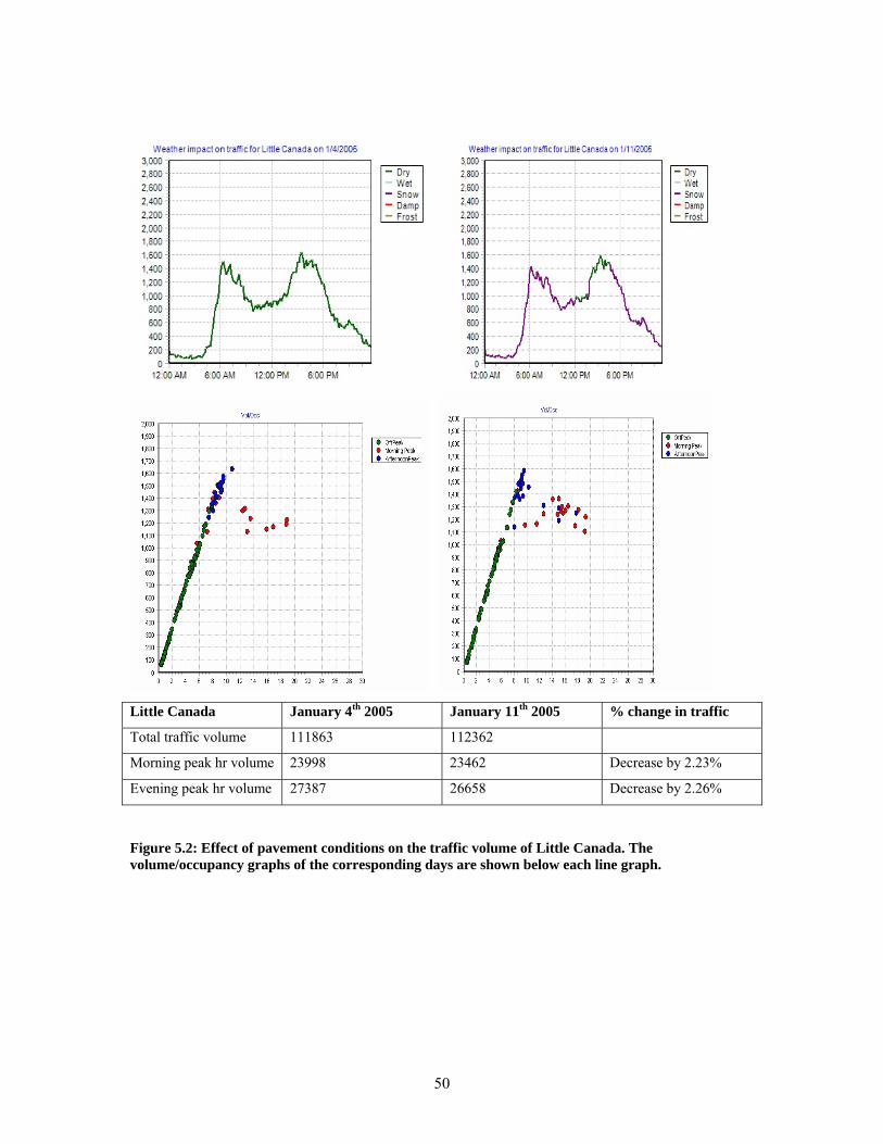
50
Little Canada January 4th 2005 January 11th 2005 % change in traffic
Total traffic volume 111863 112362
Morning peak hr volume 23998 23462 Decrease by 2.23%
Evening peak hr volume 27387 26658 Decrease by 2.26%
Figure 5.2: Effect of pavement conditions on the traffic volume of Little Canada. The volume/occupancy graphs of the corresponding days are shown below each line graph.

51
Case 2: Reduction of congestion by a severe snow event This is the case where a snow event actually reduces congestion. In this case the snow
event was severe and the volume was significantly reduced during the morning peak in comparison to a normal dry day. From Figure 5.3 right bottom, it can be clearly observed that traffic congestion was actually reduced during the snow event according to the volume/occupancy scatter graph. A logical explanation in this case is that the capacity of the freeway was reduced by snow but the volume was more significantly reduced, preventing congestion.
Little Canada January 17th 2005 January 31st 2005 % change in traffic
Total traffic volume 101698 108200
Morning peak hr volume 18596 21601 Increase by 14%
Evening peak hr volume 24924 27150 Increase by 8.1%
Figure 5.3: Effect of severe snow conditions on the traffic volume. The volume/occupancy graphs of the corresponding days are shown below each line graph.
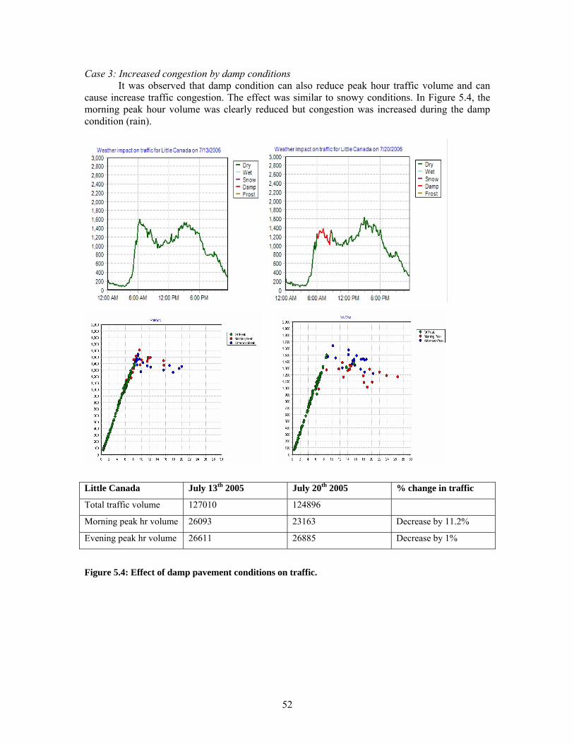
52
Case 3: Increased congestion by damp conditions It was observed that damp condition can also reduce peak hour traffic volume and can
cause increase traffic congestion. The effect was similar to snowy conditions. In Figure 5.4, the morning peak hour volume was clearly reduced but congestion was increased during the damp condition (rain).
Little Canada July 13th 2005 July 20th 2005 % change in traffic
Total traffic volume 127010 124896
Morning peak hr volume 26093 23163 Decrease by 11.2%
Evening peak hr volume 26611 26885 Decrease by 1%
Figure 5.4: Effect of damp pavement conditions on traffic.

53
Case 4: Volume decrease and increase of congestion by wet conditions
Wet conditions were investigated to see how they affect traffic volume and congestion. The graphs are shown in Figure 5.5. Similarly to damp conditions, traffic volume was reduced and congestion was increased. Also notice from the graph that congestion begins to occur at a lower volume which suggests reduction in the freeway capacity. This reduction in capacity appears to be the cause of increased congestion.
Burnsville February 2nd 2005 February 14th 2005 % change of traffic
Total traffic volume 104683 104632
Morning peak traffic 21284 19793 Decrease by 7%
Afternoon peak traffic 25003 25793 Increase by 3.1%
Figure 5.5: Effect of wet pavement conditions on traffic.
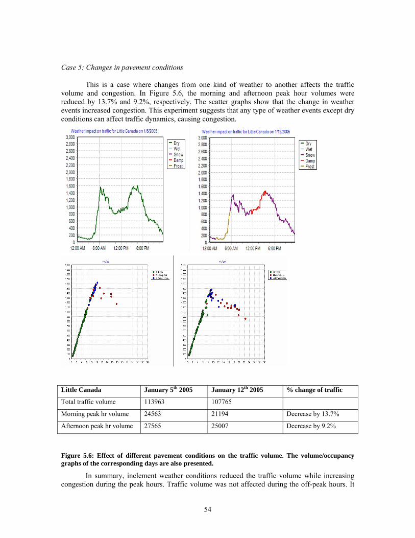
54
Case 5: Changes in pavement conditions This is a case where changes from one kind of weather to another affects the traffic
volume and congestion. In Figure 5.6, the morning and afternoon peak hour volumes were reduced by 13.7% and 9.2%, respectively. The scatter graphs show that the change in weather events increased congestion. This experiment suggests that any type of weather events except dry conditions can affect traffic dynamics, causing congestion.
Little Canada January 5th 2005 January 12th 2005 % change of traffic
Total traffic volume 113963 107765
Morning peak hr volume 24563 21194 Decrease by 13.7%
Afternoon peak hr volume 27565 25007 Decrease by 9.2%
Figure 5.6: Effect of different pavement conditions on the traffic volume. The volume/occupancy graphs of the corresponding days are also presented.
In summary, inclement weather conditions reduced the traffic volume while increasing congestion during the peak hours. Traffic volume was not affected during the off-peak hours. It

55
was also observed that if the snow conditions are very severe, the traffic volume drops considerably and the congestion was actually reduced or disappeared. The damp and wet conditions affected similarly to snow conditions but a drastic drop of volume that causes reduction in congestion was not observed. Finally, it was observed that when the traffic volume was reduced during the peak hours by weather events, more traffic volumes during the following off-peak hour were observed. This indicates that the traffic flow shifts towards non-peak hour when weather events occur.
5.5.4 Impact of inclement weather conditions on travel time prediction
In order to analyze the impact of pavement conditions on travel time prediction, a section of 17.5 miles from Maple Grove to Little Canada was used. Eq. 5.6 was used for the computation of the percentage prediction error (PPE). The hypothesis is that PPE of the time varying linear coefficient approach would be higher when inclement weather conditions impact the traffic dynamics. To analyze the travel time affected by weather conditions, line graphs for the predicted travel time and the baseline travel time estimates and its corresponding PPE values are compared. The calibrated travel time estimates (Eq. 5.5) at the same time are then plotted along with the predicted travel time and the baseline estimate of travel time to note any improvements. The weather impact on traffic volume and volume/occupancy scatter graphs are presented to show the traffic conditions.
Case-by-case analyses of various examples on weather impact on travel time are shown. In all graphs shown, the legend “TV” denotes the time varying linear coefficient approach, “Baseline” denotes actual travel time estimates, and “TVWI” denotes travel time estimates with weather impact incorporated. In the experiments, Δ was set to 5, 15, or 30 minutes, i.e., travel time prediction at 5, 15, or 30 minutes ahead. In the case studies, only the prediction examples with 15Δ = minutes are presented since the differences in performance can be more clearly observed from the graphs. The historical information of 3 hours prior to the hour of prediction was used to compute the time varying coefficients.
Case 1: Effect of travel time prediction when weather conditions do not cause congestion
As discussed in the previous section, severe snow conditions sometimes significantly
decrease the volume at which reduced capacity in the freeway is not sufficient to cause congestion. This case is shown in Figure 5.7. Once the traffic volume drops significantly, the TV travel time prediction model starts performing better since the traffic changes to a free flow state. However it can be seen from the graph that during 5:00-6:00AM the traffic volume has not dropped considerably, and thus the effect of weather impact can be seen on travel time prediction for the hour. In the TVWI model, the change in the occupancy adjusts the impact of inclement weather condition on travel time and the accuracy closely approaches the baseline. The overall effect of significant drop in traffic due to severe snow conditions is that the accuracy of travel time prediction by the TV model is well maintained. The current travel time predictor is being used to predict the travel time 15 minutes into the future (Δ=15 minutes).

56
Effect of pavement conditions on travel time prediction for 01/17/2005
500
750
1000
1250
1500
5:00
5:20
5:40
6:00
6:20
6:40
7:00
7:20
7:40
8:00
8:20
8:40
9:00
Time instance
Trav
el ti
me
in s
econ
ds
TVBaselineTVWI
Figure 5.7: Traffic is affected by severe snow conditions that reduce the volume and avoid congestion and hence facilitates free flow conditions. The percentage prediction error of travel time is also negligible.

57
Case 2: Effect of travel time prediction by before-and-after weather events
The change in the pavement conditions can cause error in the prediction of travel time as the prediction depends on the previous travel time information. If the weather event changes from dry to snow, the TV model underestimates the travel time during the snow event. To illustrate this, note from Figure 5.8 that the pavement conditions in the afternoon changes from dry conditions to snow. Congestion occurred during the afternoon peak hours. Note from the travel time performance graph that TVWI model performs better in comparison to the TV model under the change of weather conditions since it incorporates the weather conditions.

58
Figure 5.8: Travel time prediction is affected by the snow conditions which cause congestion. The PPE graph shows the error that occurs due to the change in weather.
Effect of pavement conditions on travel time prediction for 01/11/2005
500
750
1000
1250
1500
1750
15:0
0
15:2
0
15:4
0
16:0
0
16:2
0
16:4
0
17:0
0
17:2
0
17:4
0
18:0
0
18:2
0
18:4
0
19:0
0
Time instance of the day
Trav
el ti
me
in s
econ
ds
TVBaselineTVWI
Effect of calibration of weather impact on travel time prediction
-0.3-0.2
-0.10
0.10.2
0.30.4
15:00
15:25
15:50
16:15
16:40
17:05
17:30
17:55
18:20
18:45
Time instance
Perc
enta
ge p
redi
ctio
n er
ror PPETV
PPETVWI

59
Case3: Wet and damp pavement conditions in the morning peak time This case illustrates how the wet condition impacts travel time prediction. In Figure 5.9,
during the morning, peak hour traffic volume was reduced due to wet conditions but it caused congestion (significant increase of occupancy in the scatter graph). As shown in the travel time performance in the middle and bottom graphs, the TV prediction model underestimates the travel time during the weather event and overestimates immediately after the weather event. This makes sense since it predicts the travel time based on the past data. Note from the TVWI model that the rate of under- and over-estimate is significantly reduced since it incorporates the weather condition. This case again demonstrates that incorporation of weather conditions to travel time prediction improves the accuracy of prediction.

60
Figure 5.9: Travel time was affected by damp conditions. The damp conditions increased the travel time, and the TV prediction model underestimates the travel time. The TVWI model corrects the difference and improves the prediction accuracy.
Effect of pavement conditions on travel time prediction for 07/20/2005
500
750
1000
1250
1500
1750
5:00
5:20
5:40
6:00
6:20
6:40
7:00
7:20
7:40
8:00
8:20
8:40
9:00
Time instance
Trav
el ti
me
in s
econ
ds
TVBaselineTVWI
Effect of calibration of weather impact on travel time prediction
-0.4
-0.3
-0.2
-0.1
0
0.1
0.2
5:00
5:20
5:40
6:00
6:20
6:40
7:00
7:20
7:40
8:00
8:20
8:40
9:00
Time instance
Perc
enta
ge p
redi
ctio
n er
ror
PPETVPPETVWI

61
Case 4: The whole day is affected by snow
In this case (Figure 5.10), snowy conditions occurred the whole day, which affected the travel time prediction. Traffic volume indeed decreased significantly when it was compared with a normal dry day (Table 5-4), while the travel time and congestion was increased during the peak traffic hours. Note from the performance graphs in Figure 5.10 that the TV prediction model consistently underestimates the travel time in this case. The TVWI model corrects the error by incorporating the weather conditions but it still underestimates the travel time.

62
Figure 5.10: Travel time is affected by snow conditions for the whole day. The snow conditions increase the travel time and the prediction tends to underestimate the travel time.
Effect of calibration of weather impact on travel time prediction
-0.4-0.3-0.2-0.1
00.10.20.30.4
5:00
5:30
6:00
6:30
7:00
7:30
8:00
8:30
9:00
16:05
16:35
17:05
17:35
18:05
18:35
Time instance
Perc
enta
ge p
redi
ctio
n er
ror
PPETVPPETVWI
Effect of pavement conditions on travel time prediction for 01/20/2005
500750
10001250150017502000
5:00
5:30
6:00
6:30
7:00
7:30
8:00
8:30
9:00
16:05
16:35
17:05
17:35
18:05
18:35
Time instance
Trav
el ti
me
in s
econ
ds
TV
BaselineTVWI

63
Case 5: Multiple changes of weather changes during the day
In this case, weather conditions vary during the day as shown in top left line graph of Figure 5.11. The conditions changed at the Little Canada site on Jan 12th 2005 from frost to snow, snow to wet, and then wet to snow. The bottom two graphs show that the TV model underestimates the travel time during the morning peak hours and overestimates during the afternoon peak hours. This inconsistency is due to varying conditions. The TVWI model corrects this error and closely approximates to the baseline estimates.
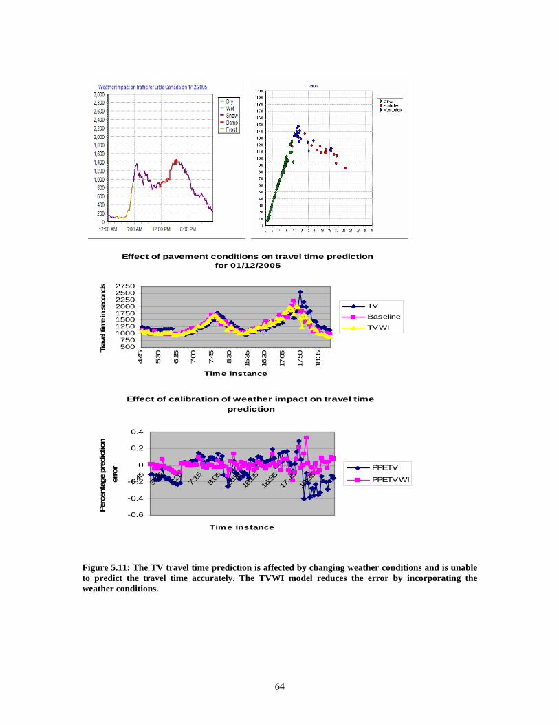
64
Figure 5.11: The TV travel time prediction is affected by changing weather conditions and is unable to predict the travel time accurately. The TVWI model reduces the error by incorporating the weather conditions.
Effect of pavement conditions on travel time prediction for 01/12/2005
500750
10001250150017502000225025002750
4:45
5:30
6:15
7:00
7:45
8:30
15:3
5
16:2
0
17:0
5
17:5
0
18:3
5
Time instance
Trav
el ti
me
in s
econ
ds
TV
Baseline
TVWI
Effect of calibration of weather impact on travel time prediction
-0.6
-0.4
-0.2
0
0.2
0.4
4:45
5:35
6:25
7:15
8:05
8:55
16:05
16:55
17:45
18:35
Time instance
Perc
enta
ge p
redi
ctio
n
erro
r PPETV
PPETVWI

65
5.6 Chapter Conclusion The chapter presented analyses on the weather impact on traffic utilizing Mn/DOT RWIS
and traffic data. According to the correlation coefficient study, no strong correlations between the traffic and RWIS parameters were found. Next, the effect of daily traffic volume was investigated. It was found that daily total volume under weather events was only marginally affected (decreased). In most cases, the peak hour traffic volume was reduced but the reduced volume appeared during the off-peak hours. In order to study how weather impacts traffic during peak hours, color coded visualization techniques were used, i.e., the traffic volume graphs were generated with different colors, representing different pavement conditions. The volume/occupancy scatter graphs were color coded according to morning and afternoon peak hours and off-peak hours. The analysis of these graphs suggests that the traffic volume generally drops during peak hours if a snow or wet weather event occurs. The drop in the traffic volume depends on the kind of weather event and the severity of the weather. It was also observed that freeway capacity was reduced under weather events. In most cases, congestion was increased during a weather event although the volume drops as well. This suggests that the weather event reduces the freeway capacity but the trip demand to use the freeway also decreases. One exception was also observed. During severe snow conditions the traffic volume dropped considerably, indicating significant reduction in trip demands. In those cases, congestion on the freeway was actually reduced in comparison to a normal dry day. The wet and damp conditions did not sufficiently reduce the trip demands enough to ease congestion, but the freeway capacity was reduced enough to cause a higher level of congestion.
As the second part, the impact of weather events on the travel time prediction was investigated using a time-varying linear coefficient (TV) model which is a basic linear prediction model. Since the TV travel time prediction model relies on the historical travel time data to estimate the future travel time, the prediction errors were more significant under changing weather conditions. It was observed that if the pavement conditions change from snow, damp, or wet to normal dry conditions then the TV model tends to overestimates the travel time. On the other hand, if the pavement conditions change from dry to snow, damp, or wet conditions then the TV model tends to underestimates the travel time. This happens because the prediction model assumes that the future travel condition is identical to the past travel condition. In this project, an attempt was made to reduce the error induced by the impact of weather changes. It was found that the changes in occupancy of the freeway under weather events, i.e., the change when the occupancy was compared to the normal dry conditions, provided adjustment factors in prediction of travel time. The calibration factor that was suggested in Eq. (5.5) is based on the change in the occupancy that would occur due to weather events. Various experiments conducted for different cases suggest that the error in the travel time prediction on the past history of traffic (e.g., the TV model) increases during weather event. This project shows that such prediction errors can be reduced if the change in estimated occupancy due to the weather event is incorporated into the model.
One of the difficulties of RWIS data is that it does not provide an index that indicates severity of a weather event. Such a measure could help formulate the drop in freeway capacity and effect on congestion, and could lead to developing a more reliable prediction model for travel or trip times under weather events. Therefore, development of a weather severity index is recommended as a future study.
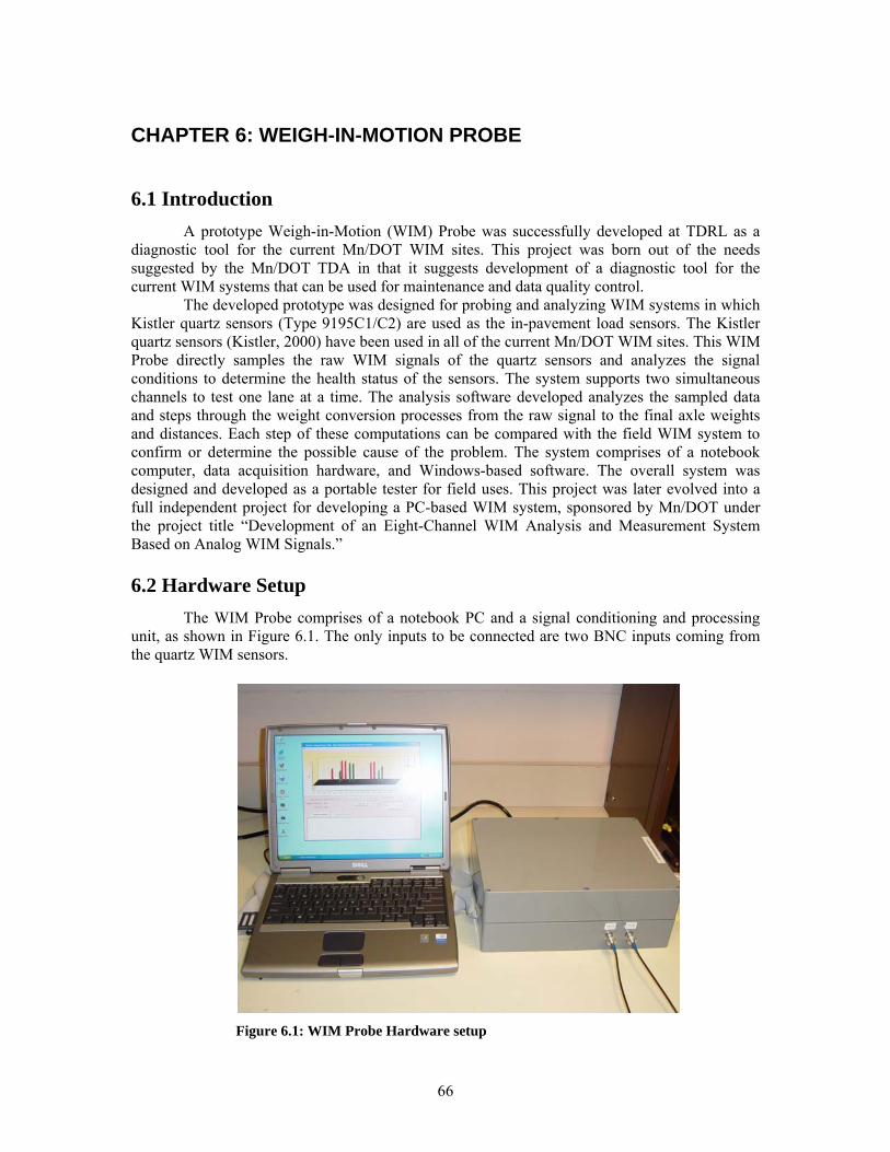
66
CHAPTER 6: WEIGH-IN-MOTION PROBE 6.1 Introduction
A prototype Weigh-in-Motion (WIM) Probe was successfully developed at TDRL as a diagnostic tool for the current Mn/DOT WIM sites. This project was born out of the needs suggested by the Mn/DOT TDA in that it suggests development of a diagnostic tool for the current WIM systems that can be used for maintenance and data quality control.
The developed prototype was designed for probing and analyzing WIM systems in which Kistler quartz sensors (Type 9195C1/C2) are used as the in-pavement load sensors. The Kistler quartz sensors (Kistler, 2000) have been used in all of the current Mn/DOT WIM sites. This WIM Probe directly samples the raw WIM signals of the quartz sensors and analyzes the signal conditions to determine the health status of the sensors. The system supports two simultaneous channels to test one lane at a time. The analysis software developed analyzes the sampled data and steps through the weight conversion processes from the raw signal to the final axle weights and distances. Each step of these computations can be compared with the field WIM system to confirm or determine the possible cause of the problem. The system comprises of a notebook computer, data acquisition hardware, and Windows-based software. The overall system was designed and developed as a portable tester for field uses. This project was later evolved into a full independent project for developing a PC-based WIM system, sponsored by Mn/DOT under the project title “Development of an Eight-Channel WIM Analysis and Measurement System Based on Analog WIM Signals.”
6.2 Hardware Setup
The WIM Probe comprises of a notebook PC and a signal conditioning and processing unit, as shown in Figure 6.1. The only inputs to be connected are two BNC inputs coming from the quartz WIM sensors.
Figure 6.1: WIM Probe Hardware setup
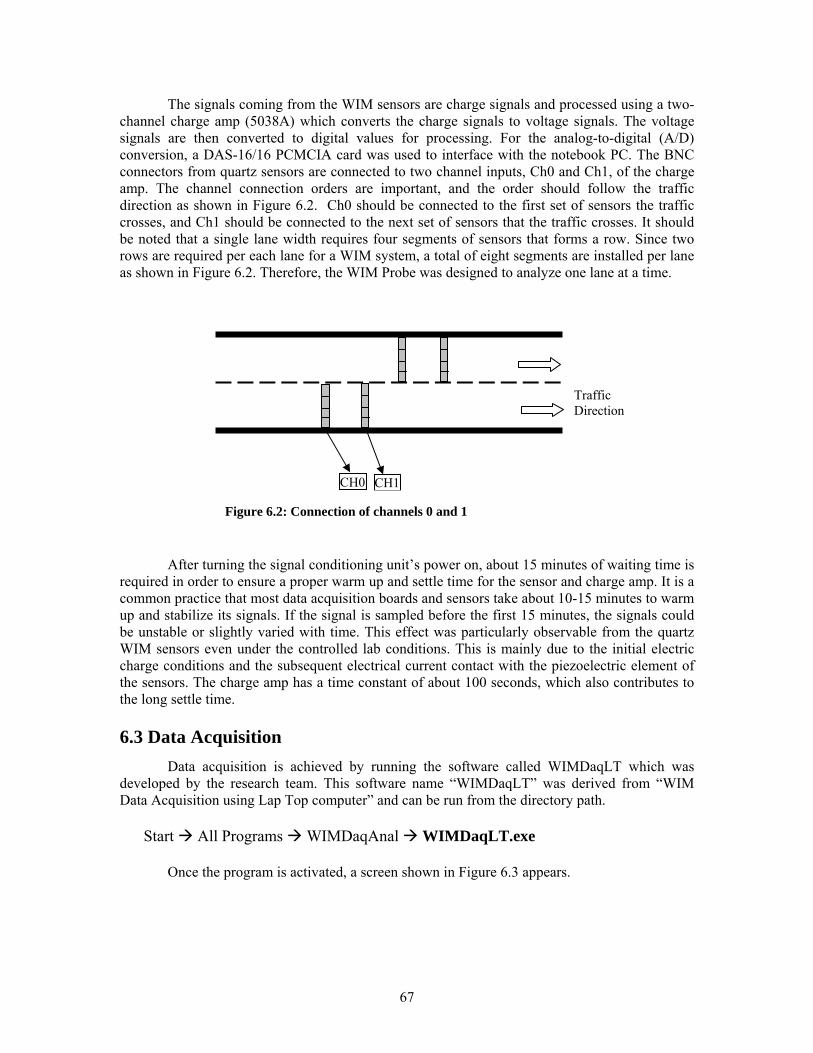
67
The signals coming from the WIM sensors are charge signals and processed using a two- channel charge amp (5038A) which converts the charge signals to voltage signals. The voltage signals are then converted to digital values for processing. For the analog-to-digital (A/D) conversion, a DAS-16/16 PCMCIA card was used to interface with the notebook PC. The BNC connectors from quartz sensors are connected to two channel inputs, Ch0 and Ch1, of the charge amp. The channel connection orders are important, and the order should follow the traffic direction as shown in Figure 6.2. Ch0 should be connected to the first set of sensors the traffic crosses, and Ch1 should be connected to the next set of sensors that the traffic crosses. It should be noted that a single lane width requires four segments of sensors that forms a row. Since two rows are required per each lane for a WIM system, a total of eight segments are installed per lane as shown in Figure 6.2. Therefore, the WIM Probe was designed to analyze one lane at a time.
After turning the signal conditioning unit’s power on, about 15 minutes of waiting time is required in order to ensure a proper warm up and settle time for the sensor and charge amp. It is a common practice that most data acquisition boards and sensors take about 10-15 minutes to warm up and stabilize its signals. If the signal is sampled before the first 15 minutes, the signals could be unstable or slightly varied with time. This effect was particularly observable from the quartz WIM sensors even under the controlled lab conditions. This is mainly due to the initial electric charge conditions and the subsequent electrical current contact with the piezoelectric element of the sensors. The charge amp has a time constant of about 100 seconds, which also contributes to the long settle time. 6.3 Data Acquisition
Data acquisition is achieved by running the software called WIMDaqLT which was developed by the research team. This software name “WIMDaqLT” was derived from “WIM Data Acquisition using Lap Top computer” and can be run from the directory path.
Start All Programs WIMDaqAnal WIMDaqLT.exe
Once the program is activated, a screen shown in Figure 6.3 appears.
Traffic Direction
CH0 CH1
Figure 6.2: Connection of channels 0 and 1

68
Figure 6.3: WIMDaqLT.exe initial screen
WIM data acquisition from quartz sensors is then achieved by following the steps
described below. 1. Choose the sampling rate.
The default value is set to 3,000 samples per second (S/s), which would be sufficient for WIM. A sampling rate, 4,090 S/s, could also be selected for more accurate measurements.
2. Press the “Start Signal Scan Operation” button. Data is always sampled from both channels (Ch0 and Ch1) simultaneously, but one can choose to display one channel at a time or simultaneously by removing or setting the check marks on the graph legend. Once sampling starts, the start button is changed to a stop button and the label is changed to “Stop Signal Scan Operation.” At the same time, the Quit button and Sampling Rate combo-buttons are disabled to prevent inadvertently activating them. In order to change the sampling rate or to quit the program, the signal sampling (scanning) operation must be stopped first.
3. Record the data by pressing the Start button on the File Recording group. The sampled raw data (binary format) is stored at “C:\Program Files\WIMDaqAnalysis\DataAcquisition\yyyymmdd” where yyyymmdd is the directory name automatically created based on the time of sampling date, i.e., year, month, and day. The raw data file is automatically created with the name hhmmss_SamplingRate.bin where hhmmss is the starting time of the data acquisition. For example, if the sampling was started at 14:05:20 with 3,000 Samples/sec, the file name would be 140520_3000.bin. Each data file stores up to 20 seconds worth of data, and if the data size exceeds this limit, another file is automatically created for the next 20 seconds of data. This process repeats until the user presses the Stop button on the File Recording group. The number of files that have been recorded are shown in the File Recording Status with the format ##:## (number of files: number of seconds). Once recording starts, the signal scan operation button is disabled because the data cannot be recorded without sampling. The user must first stop the recording in order to stop the signal scan operation.
4. Stop recording data by pressing the Stop button on the File Recording group.

69
As soon as the Stop button is pressed, the WIM data recording stops after completing savings of the current data in order to make sure that a proper boundary of the data is stored in the recorded data. During the data acquisition, the signal is plotted using a real-time line graph display. The
plot range can be selected during any time during the data acquisition process by selecting a choice out of “–1V to +3V”, “-1V to +5V”, and Auto. Auto range means plot of the data between the maximum and minimum of the data range within the window. The x-axis labels denote sampling indices, e.g., for sampling rate 3,000 S/s, the first window indices are 0-2999, the second window indices are 3000-5999, etc. After recording the data, the binary data can be converted to ASCII strings using the Analysis tool. It produces a standard comma separated value format, and the resulting file can be directly loaded into MS Excel.
6.4 Data Analysis After completion of data acquisition, the captured data is analyzed using another tool
called DataAnal. This tool provides visualization of WIM electric signal, measurements of idle level noise, computation of axle distances, and finally computation of axle and vehicle weights. 6.4.1 Data navigation
The software user interface is shown in Figure 6.4. Once the data is loaded, all data control buttons are enabled and the data can be navigated using the following buttons in the middle section of the display, which are explained below.
move to the next data window move to the previous data window ->> move two data windows forward <<- move two data windows backward ->| move to the end of data |<- move to the beginning of data “Show All” show all data using a slide show Data Y-range may be changed using the slide bars or Set Auto Range. The number of data points to be displayed per window can be changed by setting the
value at the Block Size text box and clicking the Set button. It is useful when details of signal need to be observed are partially outside the window.
The legends of the graphs are:
Ch0 --- channel 0 raw data Ch1 --- channel 1 raw data Ch0V --- channel 0 raw data after wheel detection Ch1V --- channel 1 raw data after wheel detection

70
Figure 6.4: Data Analysis Screen
6.4.2 Axle signal analysis and weight computation
In Figure 6.4, weight signals for a class-9 five-axle truck are shown. As the first step of signal processing, the axle signals must be separated from the idle signal. The signal level of the sensor with no load is called the idle signal. Since the idle signal is not a constant, an adaptive method is used to continuously track the signal level. In the Figure 6.4 user interface, axle signals are extracted by pressing the “Extract Vehicle” button.
After axle extraction, a clustering algorithm runs and determines which axle signal belongs to which vehicle. The detected wheels are then indexed for both channels and the measurements are displayed on the three tables in the bottom window (see Figure 6.5). Intermediate data files are stored for analysis in the directory “C:\Program Files\WIMDaqAnalysis\Analysis\”. The file types and data format of the intermediate files are summarized in Table 6-1. The user can use theses data files for diagnostics, such as checking noise level, idle level, signal integrity for each axle, etc.

71
Table 6-1: Output Files and Data Format
Speed.txt Speed estimation using wheel footprints used by the algorithm. It is not the actual speed but is a computation of [0.17 * (Sample rate)/(Width count)] which is a rough initial estimate.
Wheels.txt This file provides all of the measurements for each wheel and the channel. The data is also displayed in the table window. The data fields of this file are:
Data Field Description whIndex The index that identifies a wheel BeginI Sample instant index of the start of the wheel footprintEndI Sample instant index of the end of the wheel footprint maxIndex Sample instant index where maximum voltage is
observed within the footprint of the wheel maxValue The voltage at the maxIndex Area Sum of all voltage values under the curve of each
wheel IdleLevel The voltage level between wheels. If this level is not
close to zero, the sensor may have a hardware problem.
noiseLevel The noise level is computed for the idle period by computing mean square root error of the signal level. This value is always positive and should be close to zero, otherwise it indicates that the sensor is experiencing a noise problem.
VehWheels.txt This file shows which wheel belongs to which vehicle. Wheels are expressed using the wheel index found in wheels.txt file. Vehicles are indexed starting from 0. Each vehicle occupies one row with the corresponding wheel indices.
The next step of analysis is computing speed, axle distances, axle weights, and the vehicle weight by pressing the “Compute Weight” button. These values are computed using the axle data derived from Step 2. Since the data is available from both channels, two computational results are available and can be compared. This data is also shown in the bottom table of the display and is saved in a text file “vehRecord.txt” in the analysis directory “C:\Program Files\WIMDaqAnalysis\Analysis\”. The data fields of the computed results are recorded with the column format shown in Table 6-2. The accuracy of a WIM system can then be measured by driving a vehicle with known weight and axle distances through the sensor and by comparing the known values with the recorded data.

72
Figure 6.5: Completed data window
Table 6-2: WIM Parameter Columns
Data Field Description vehIndex Vehicle indexed starting from 0 DateTime The date and time of the vehicle which crossed the sensor mph Speed in mph WheelWeights Wheel weights in pounds. Each wheel is separated by “-“ For example, 5 axle
vehicle is expressed as 4717-6067-5833-3847-5487. For screen, 4717=6067=5833=3847=5487.
TotalWeight Sum of each wheel weights in pounds axleDistances Axle distances in feet. Each axle distance is separated by “-“. For screen
display, “=” is used in place of “-“. 6.4.3 Weight Calibration
The weight is computed using the calibration factor derived from a typical factory setting
of the sensor sensitivity. This value drifts over time and requires calibration. The software has a utility routine for this calibration and the steps are described below. Step 1: Collect data using a vehicle with a known weight. The software uses the first vehicle detected from the data set. Step 2: Under the file menu, select “Calibrate Weight” item, which will open up the following dialog window.

73
Step 3: Enter the known weight of the first vehicle detected in the blank Step 4: Press the Calibrate button and then Exit. This completes the calibration.
Once the calibration is completed, the calibration factor is affected from the next weight computation. Since this calibration factor is kept in the Windows registry, its value is kept in computer even if the program is exited or the computer is turned off. If mistakes were made, one can always go back to the factory default setting by clicking the “Set Default” button. 6.5 Static Weight Test Tool
This tool is used for testing the quartz sensors before installing in the pavement. In order to use this tool, the BNC connector from a quartz sensor is directly connected to one of the channels Ch0 or Ch1 of the WIM Prob. A program named, “StaticWeight,” is then activated. A sample screen of this tool is shown in Figure 6.6. It displays the weight converted values sampled from the channel selected; the actual voltage level is monitored; and the idle level is traced from the signal. A simple way of using this tool is using a person’s weight since most people know their approximate weight. The user simply steps on to the quartz sensor like a bathroom scale and then reads the weight shown on the screen. If the quartz sensor works correctly, the weight reading should be close to the known weight.
Figure 6.6: Static weight testing tool

74
The weight is computed using the conversion factor derived based on the sensitivity of the quartz sensor measured in factory (Figure 6.7). The default conversion factor computed from the Kistler value is 706.88. One can edit the conversion factor while it displays the weights. Increasing this value increases the weight values and decreasing it decreases the weight values since the conversion factor is multiplied by the measured sensor voltage. An example screen is shown in Figure 6.6 which uses Ch0. The Start and Stop button works as a toggle button. To exit the program, the Stop button must be pressed first and then the Quit button.
Figure 6.7: Factory sensitivity setting specified on the sensor
6.6 Signal Anomalies and Treatments As a usage example of the WIM Probe, two common signal error conditions frequently
observed from the field WIM sites and their treatments are described in this section. The first commonly observed problem is the piezoelectric recovery error. An ideal WIM
sensor should not produce any charges as soon as the wheel leaves the sensor. However, since the piezoelectric sensor produces charges in response to the changes in the sensor’s physical structure, the charges are generated until the physical structure is completely restored. Unfortunately, the physical structure often does not return to the original state fast enough, producing a long tail in the axle signal. Two examples are shown: a mild case in Figure. 6.8 and a severe case in Figure 6.9. The remedy for this problem is to use only the first half portion of the signal (i.e. up to the peak) during the weight computation process. The total weight is then simply obtained by doubling the first half. This method works as long as the speed of the vehicle remains the same for the duration of the wheel foot print. This recovery error also occurs when small rock fragments are wedged between the pavement and the wall of the WIM sensor. Clearing these rock fragments can resolve the large piezoelectric recovery error.

75
Figure 6.8: WIM signal with piezoelectric recovery problem
Figure 6.9: A severe case of piezoelectric recovery problem.
As with most analog signals, line noise can be introduced in the WIM signal. Figure 6.10
shows an example of line noise observed from one of the Mn/DOT WIM sites. One serious problem caused by these line noises is a false detection of threshold, which would end up accepting a noise spikes as an axle signal. In order to reduce the line noise, coaxial cables are generally used for connecting WIM sensors. However, if any leakage occurs from the outer shield layer of the coaxial cable, noise can be introduced. The shield leakage often occurs within the line splice or from the damaged spots in the shield layer. One remedy to this problem is to set the threshold level higher than the line noise level by measuring the variance of the noise. It was also found that the amplitude of axle signals increases as the level of line noise increases. This makes sense because axle signals are essentially an integrated signal converted by a charge amp. Therefore, amplitude adjustments in axle signals are needed with respect to the line noise. To remove the line noise, several low-pass filtering techniques were tested, but that resulted in distortion of axle signals without compensating the amplification effects caused by the noise. One approach that worked reasonably well was to scale down the axle signals proportional to the noise standard deviation. However, the signal processing solution has only limited effects, and the best solution would be physically repairing the line by wrapping shielding tapes.
Figure 6.10: Line noise

76
6.7 WIM Probe Technical Information The technical information for the developed WIM Probe is summarized below:
A/D Maximum Sampling Rate: 100 K Samples per second A/D Sample Resolution: 16 bit Data Acquisition Card Model: PCMCIA-Card DAS16/16 Voltage Sampling Range: -5V to + 5V Number of Channels: 2 Each Channel Sampling Rate: 3,000 or 4,090 Charge Amplifier: Kistler 5038A2Y43 Measurement Range of Piezoelectric Charge: ±60,000 pC Time Constant of Charge Amp: 100 seconds
6.8 Concluding Remarks
This chapter described the functions of the prototype WIM Probe developed as a diagnostic tool for the presently installed WIM sites at Mn/DOT. This tool can be used to probe the signal characteristics of WIM sensors, to test computational results of a WIM system, as well as verification of sensor quality before installing quartz WIM sensors on the pavement. Because data quality of WIM systems is sensitive to the sensor signal quality, it is important to maintain the sensors to work within the electrical specification. However, no convenient tools have been available. This tool fills that need and provides reading of raw analog signals and various analysis steps, which should help improve the data quality of WIM stations.

77
References
[1] Archived Data User Service (ADUS), “ITS Data Archiving: Five-Year Program Description,” March 2000, Published by U.S. DOT, ADUS Program. [2] Box, G.E.P., G.M. Jenkins, and G.C. Reinsel, Time Series Analysis – Forecasting and Control, 3rd ed., Englewood Cliffs, NJ; Prentice Hall, 1994. [3] Chatfield, C., The Analysis of Time Series – An Introduction, 5th ed., London, UK; Chapman and Hall, 1996. [4] Chen C., K. Petty, A. Skabardonis, and P. Varaiya, “Freeway Performance Measurement System: Mining Loop Detector Data,” Transportation Research Record 1748, TRB, Washington, D.C., 2001, pp 96-102. [5] Chen C., J. Kwon, J. Rice, A. Skabardonis, and P. Varaiya, “Detecting Errors and Imputing Missing Data for Single Loop Surveillance Systems,” TRB 82nd Annual Meeting CD-ROM, Washington, D.C., Jan 2003. [6] Cleghorn D., F. Hall, D. Garbuio, “Improved Data Screening Techniques for Freeway Traffic Management Systems,” Transportation Research Record 1320, TRB, Washington, D.C., 1991, pp 17-31. [7] Coifman B., “Using Dual Loop Speed Traps to Identify Detector Errors,” Transportation Research Record 1683, TRB, Washington, D.C., 1991, pp 47-58. [8] Cortes, C. E, Lavanya, R., Oh, J., Jayakrishnan, R. (2001), “A general purpose methodology for link travel time estimation using multiple point detection of traffic,” Technical Report, Department of Civil Engineering and institute of transportation studies, University of California, Irvine, 2001. [9] Dahlin C, “Proposed Method for Calibrating Weigh-in-Motion Systems and for Monitoring That Calibration Over Time,” Journal of the Transportation Research Board: Transportation Research Record 1364, pp. 161-168, National Academy of Science. [10] Daily D. J., Improved Error Detection for Inductive Loop Sensors, WA-RD 3001 Washington State Department of Transportation, May 1993. [11] Devore, J. L., Probability and Statistics for Engineering and the Sciences, 4th Ed, Brooks/Cole Publishing Company, CA, USA, 1995. [12] Edwards M. “How to build and profit,” Communication News, Vol. 32, No. 11 (November 1995), 49. [13] Fairhead, Neal. “Data warehousing,” Business Quarterly, Vol. 60, No. 2 (January 1995), 89 - 94.
78
[14] FHWA, Traffic Detector Handbook, 2nd Edition, FHWA-IP-90-002, Research Development and Technology, Turner-Fairbank Highway Research Center, McLean, Virginia, July 1990 [15] Fogarty K. “Data mining,” Network World, Vol. 11, No. 23 (June 1994a), 40-43. [16] Gelman A., J. Carlin, H. S. Stern, and D. B. Rubin, Bayesian Data Analysis, Texts in Statistical Science, Chapman & Hall/CRC, 1995. [17] Gold D., S. Turner, B. Gajewski and C. Spiegelman, “Imputing Missing Values in ITS Data Archives for Intervals Under 5 Minutes,” TRB 80th Meeting CD- ROM, Paper No. 01-2760, 2001. [18] Goucher, G.C. and Mathews S.S., “A Comprehensive Look at CDF,” NSSDC/WDC-A-R&S 94-07, NASA/Goddard Space Flight Center, August 1994. [19] Gajewski B., Turner S., Eisele W., and Spiegleman C., “ITS Data Archiving: Statistical Techniques for Determining Optimal Aggregation Widths for Inductance Loop Detector,” TRB 2000, Washington DC, Jan 2000. [20] HDF: http://hdf.ncsa.uiuc.edu, The HDF Group, National Center for Supercomputing Applications (NCSA), 1990. [21] Huffman, D. A., “A Method for the Construction of Minimum Redundancy Codes”, Proceedings of the Institute of Radio Engineers, September 1952, Volume 40, Number 9, pp. 1098-1101. [22] Jacobson L., N. Nihan, and J. Bender, “Detecting Erroneous Loop Detector Data in a Freeway Traffic Management System,” Transportation Research Record 1287, TRB, Washington, D.C., 1990, pp 151-166. [23] James, I.W., “The Inductive Loop Vehicle Detector: Installation Acceptance Criteria and Maintenance Techniques,” California Department of Transportation, Sacramento Transportation Laboratory, Sacramento California, Federal Highway Administration, Washington, D.C., March 1976. [24] NCHRP, “A guidebook for performance-based transportation planning,” NCHRP Report 446, National Cooperative Highway Research Program. [25] Kistler Instrument Corp., “Signal Processing Requirements for WIM LINEAS Type 9196,” 20.218e 6.00 Kistler Application Note, Winterthur, Switzerland, 2000. [26] Kwon T.M. and Dhruv N., “Unified Transportation Sensor Data Format (UTSDF) for Efficient Archiving and Sharing of Statewide Transportation Sensor Data,” Proc. of the Transportation Research Board 83rd Annual Meeting, Washington D.C., Jan. 2004. [27] Kwon, T. M., TMC Traffic Data Automation for Mn/DOT’s Traffic Monitoring Program, Mn/DOT; Report No. MN-RC-02004-29, Minnesota Department of Transportation, July 2004.

79
[28] Kwon T.M, Dhruv N., Patwardhan S., “Common Data Format Archiving of Large-Scale Intelligent Transportation Systems Data for Efficient Storage, Retrieval, and Portability,” Journal of the Transportation Research Board: Transportation Research Record 1836, pp. 111-117, National Academy of Science, 2003. [29] Kwon T.M. and Fleege S., “R/WIS Architecture for Integration and Expansion,” Journal of the Transportation Research Board: Transportation Research Record 1700, pp. 1-4, The National Research Council, The National Academies, 2000. [30] Ladaga J., “Let business goals drive your data warehouse effort,” Health Management Technology, Vol. 16, No. 11 (October 1995), 26-28. [31] Margiotta R, ITS as a Data Resource: Preliminary Requirements for a User Service. Report FHWA-PL-98-031, Federal Highway Administration, Washington, DC, April 1998. [32] Oppenheim A.V., A.S. Willsky, Ian T. Young, Signals and Systems, Prentice-Hall, Inc., Englewood Cliffs, New Jersey, 1983. [33] Little, R. J. A. and D. B. Rubin, Statistical Analysis with Missing Data, Wiley Series in Probability and Mathematical Statistics, 1987. [34] Naidu, P.S., Modern Spectrum Analysis of Time Series, Boca Raton, FL; CRC Press Inc., 1996. [35] Peeta S. and I. Anastassopoulos, “Automatic Real-Time Detection and Correction of Erroneous Detector Data Using Fourier Transforms for On-line Traffic Control Architectures,” TRB 81st Annual Meeting CD-ROM, Washington, D.C., Jan 2002. [36] Rubin, Donald B., Multiple Imputation For Non-Response in Surveys, Wiley Series in Probability and Mathematical Statistics, 1987. [37] Schafer, J. L., Analysis of Incomplete Multivariate Data, Chapman & Hall/CRC Publication, 1997. [38] Schmoyer, R., P. Hu, and R. Goeltz, “Statistical Data Filtering and Aggregation to Hour Totals of ITS Thirty-Second and Five-Minute Vehicle Counts,” TRB 80th Annual Meeting CD-ROM, Paper No 1769, 2001. [39] Smith B., D. Lewis, R. Hammond, “Design of Archival Traffic Databases: Quantitative Investigation into Application of Advanced Data Modeling Concepts,” Journal of the Transportation Research Board: Transportation Research Record 1836, pp. 126-131, National Academy of Science, 2003. [40] B.L. Smith, W. T. Scherer, J. H. Conklin, “Exploring Imputation Techniques for Missing Data in Transportation Management Systems,” Transportation Research Record 1836, TRB, Washington, D.C., 2003, pp 132-142.

80
[41] Treinish, L.A., “Data Structures and ‘Access Software for Scientific Visualization,” A Report on a Workshop at Siggraph’90, Computer Graphics, 25, No. 2, April 1991. [42] Treinish, L.A. and Goucher G.W., “A Data Abstraction for the Source-Independent Storage and Manipulation of Data,” National Space Science Data Center Technical Paper, NASA/Goddard Space Flight Center, August 1988. [43] Treinish, L.A. and Gough M.L., “A Software Package for the Data-Independent Storage of Multi-Dimensional Data,” EOS Transactions, American Geophysical Union, 68, pp. 633-635, 1987. [44] Tuner, S.M., Eisele, W.L., Gajewski, B.J., Albert, L.P., and Benz, R.J., ITS Data Archiving: Case Study Analysis of San Antonio TransGuide Data. Report FHWA-PL-99-024, Federal Highway Administration, Texas Transportation Institute, College Station, Texas, August 1999. [45] Wall J., and D.J. Daily, “An Algorithm for the Detection and Correction of Errors in Archived Traffic Data,” TRB 82nd Annual Meeting CD-ROM, Washington, D.C., Jan 2003. [46] Warner, R. M., Spectral Analysis of Time-Series Data, New York, NY; Guilford Press, 1998. [47] Zhang, X., Rice, J. A., Short Term Travel Time Prediction Model using Time Varying Coefficient Linear Model, Elsevier Reprint, March 2001. [48] Ziv J. and Lempel A., “A Universal Algorithm for Sequential Data Compression”, IEEE Transactions on Information Theory, Vol. 23, No. 3, pp. 337-343, 1977.