Transportation and Transshipment Problemsvkostogl/en/files/Educational...
62
1 TRANSPORTATION AND TRANSSHIPMENT PROBLEMS - V. Kostoglou Transportation and Transshipment Problems Vassilis Kostoglou E-mail: [email protected] URL: www.it.teithe.gr/~vkostogl/en
Transcript of Transportation and Transshipment Problemsvkostogl/en/files/Educational...
1
TRANSPORTATION AND TRANSSHIPMENT PROBLEMS - V. Kostoglou
Transportation and Transshipment Problems
Vassilis Kostoglou
E-mail: [email protected] URL: www.it.teithe.gr/~vkostogl/en

2
TRANSPORTATION AND TRANSSHIPMENT PROBLEMS - V. Kostoglou
Description A transportation problem basically deals with finding the best way to fulfill the demand of n demand points using the capacities of m supply points. While trying to find this optimal combination, a variable cost of shipping the product from one supply point to a demand point or a similar constraint should be taken into consideration.
3
TRANSPORTATION AND TRANSSHIPMENT PROBLEMS - V. Kostoglou
Transportation model Companies or manufacturers produce products at locations called sources and
ship these products to customer locations called destinations.
Each source has a limited quantity that can ship and each customer-destination has to receive a required quantity of the product.
The only possible shipments are those directly from a source to a destination. A problem with the above characteristics is generally called transportation problems. These problems involve the shipment of a homogeneous product from a number of
supply locations to a number of demand locations.
4
TRANSPORTATION AND TRANSSHIPMENT PROBLEMS - V. Kostoglou
A typical transportation problem requires three sets of information:
Capacities (or supplies)
Indicate the maximum amount most each plant can supply in a given time period.
Demands (or requirements)
They are typically estimated from some type of forecasting model. The demand
estimations are often based on historical customer demand data.
Unit shipping (or possibly production) cost
It is calculated through a transportation cost analysis.
5
TRANSPORTATION AND TRANSSHIPMENT PROBLEMS - V. Kostoglou
The transportation problem involves the determination of the amount of goods that
have to be transported from a number of sources to a number of destinations.
The most usual objective is to minimize the total shipping costs or the total
distances that have to be traveled for the transportation of the goods.
The transportation problem is a specific case of Linear Programming problems and
a special algorithm has been developed to solve it.
The problem "Given the needs at the demand locations, how should we take the limited supply at supply locations and move the goods. The objective is to minimize the total transportation cost."
6
TRANSPORTATION AND TRANSSHIPMENT PROBLEMS - V. Kostoglou
Basic concept Objective: Minimize cost Variables: Quantity of goods shipped from each supply point to each demand point Restrictions:
- Non negative shipments - Supply availability in each supply location - Demand need in each demand location
7
TRANSPORTATION AND TRANSSHIPMENT PROBLEMS - V. Kostoglou
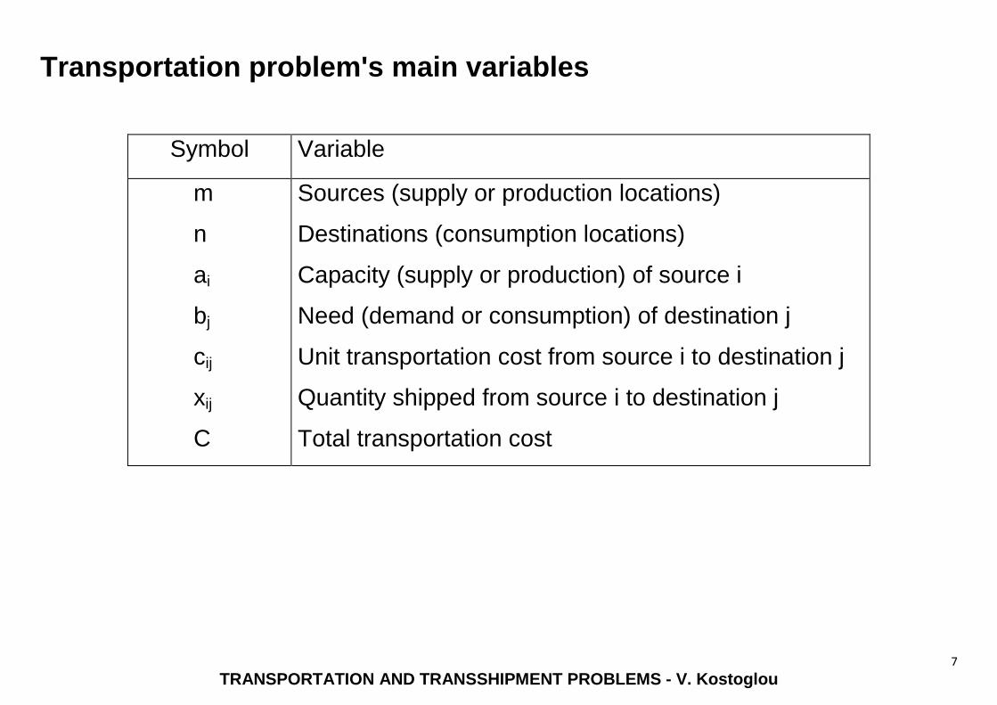
Transportation problem's main variables
Symbol Variable
m
n
ai
bj
cij
xij
C
Sources (supply or production locations)
Destinations (consumption locations)
Capacity (supply or production) of source i
Need (demand or consumption) of destination j
Unit transportation cost from source i to destination j
Quantity shipped from source i to destination j
Total transportation cost
8
TRANSPORTATION AND TRANSSHIPMENT PROBLEMS - V. Kostoglou
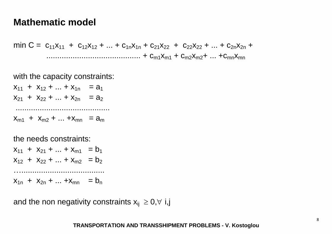
Mathematic model
min C = c11x11 + c12x12 + ... + c1nx1n + c21x22 + c22x22 + ... + c2nx2n +
........................................... + cm1xm1 + cm2xm2+ ... +cmnxmn
with the capacity constraints:
x11 + x12 + ... + x1n = a1
x21 + x22 + ... + x2n = a2
...........................................
xm1 + xm2 + ... +xmn = am
the needs constraints:
x11 + x21 + ... + xm1 = b1
x12 + x22 + ... + xm2 = b2
…......................................
x1n + x2n + ... +xmn = bn
and the non negativity constraints xij 0, i,j
9
TRANSPORTATION AND TRANSSHIPMENT PROBLEMS - V. Kostoglou
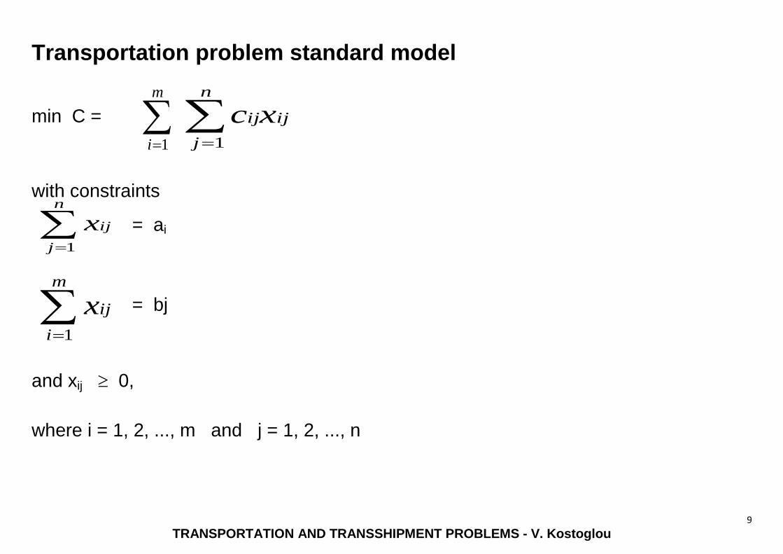
Transportation problem standard model
min C =
with constraints
= ai
= bj
and xij 0,
where i = 1, 2, ..., m and j = 1, 2, ..., n
m
i 1
n
j
ijijxc1
m
i
ijx1
n
j
ijx1
10
TRANSPORTATION AND TRANSSHIPMENT PROBLEMS - V. Kostoglou
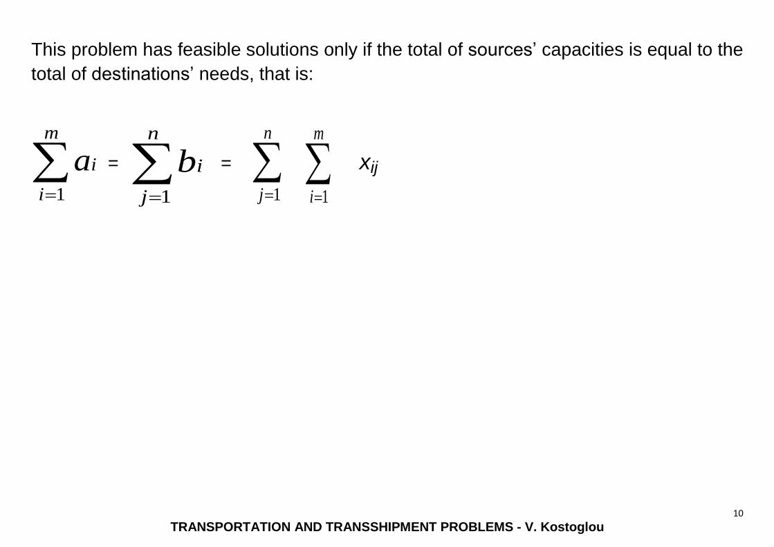
This problem has feasible solutions only if the total of sources’ capacities is equal to the
total of destinations’ needs, that is:
= = xij
m
i
ia1
n
j
ib1
n
j 1
m
i 1
11
TRANSPORTATION AND TRANSSHIPMENT PROBLEMS - V. Kostoglou
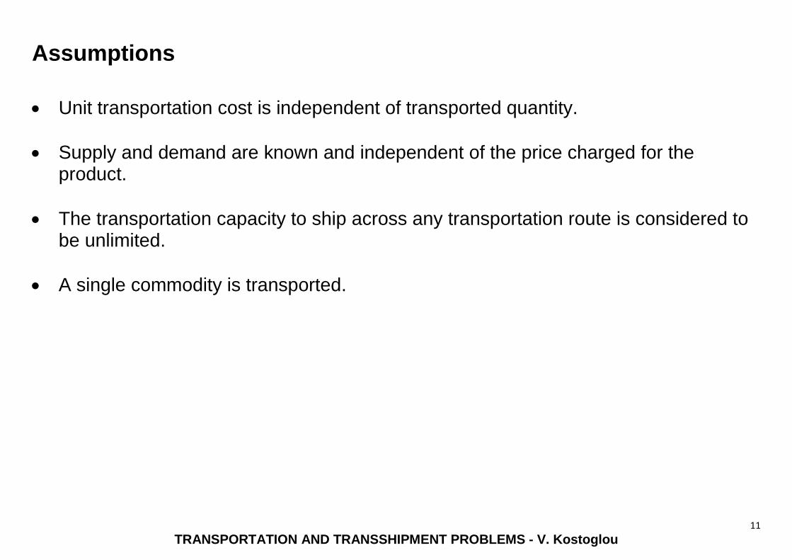
Assumptions
Unit transportation cost is independent of transported quantity.
Supply and demand are known and independent of the price charged for the product.
The transportation capacity to ship across any transportation route is considered to be unlimited.
A single commodity is transported.
12
TRANSPORTATION AND TRANSSHIPMENT PROBLEMS - V. Kostoglou
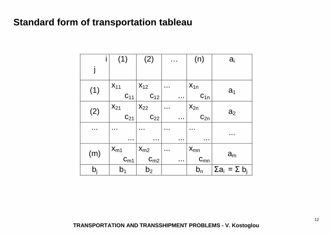
Standard form of transportation tableau
i
j
(1) (2) … (n) ai
(1) x11
c11
x12
c12
...
...
x1n
c1n a1
(2) x21
c21
x22
c22
...
...
x2n
c2n a2
...
...
...
...
...
...
...
...
... ...
(m) xm1
cm1
xm2
cm2
...
...
xmn
cmn am
bj b1 b2 bn Σai = Σ bj
13
TRANSPORTATION AND TRANSSHIPMENT PROBLEMS - V. Kostoglou
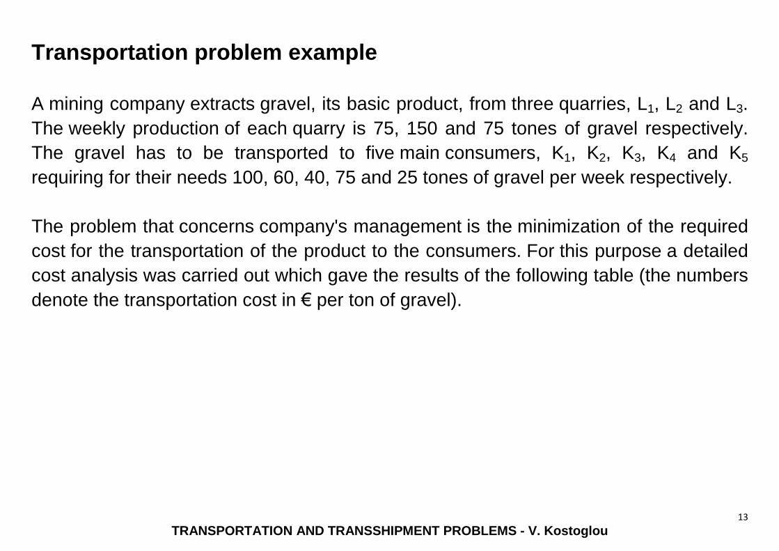
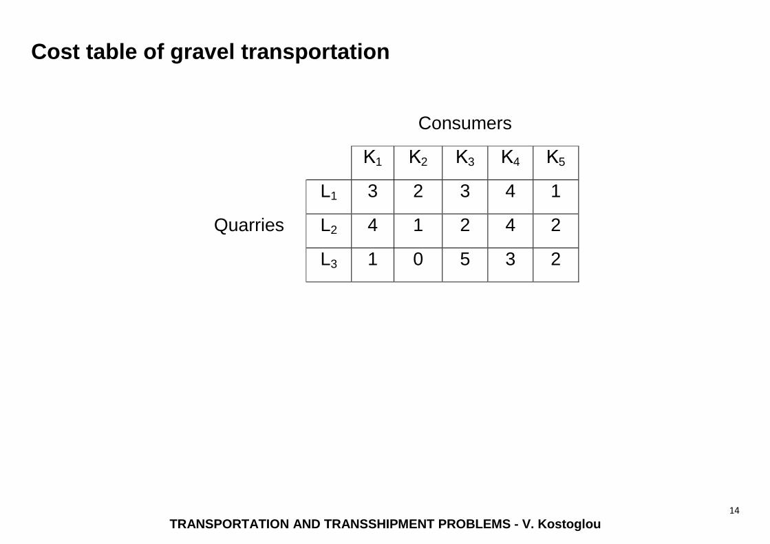
Transportation problem example
A mining company extracts gravel, its basic product, from three quarries, L1, L2 and L3.
The weekly production of each quarry is 75, 150 and 75 tones of gravel respectively.
The gravel has to be transported to five main consumers, K1, K2, K3, K4 and K5
requiring for their needs 100, 60, 40, 75 and 25 tones of gravel per week respectively.
The problem that concerns company's management is the minimization of the required
cost for the transportation of the product to the consumers. For this purpose a detailed
cost analysis was carried out which gave the results of the following table (the numbers
denote the transportation cost in € per ton of gravel).
14
TRANSPORTATION AND TRANSSHIPMENT PROBLEMS - V. Kostoglou
Cost table of gravel transportation
Consumers
Κ1 Κ2 Κ3 Κ4 Κ5
L1 3 2 3 4 1
Quarries L2 4 1 2 4 2
L3 1 0 5 3 2
15
TRANSPORTATION AND TRANSSHIPMENT PROBLEMS - V. Kostoglou
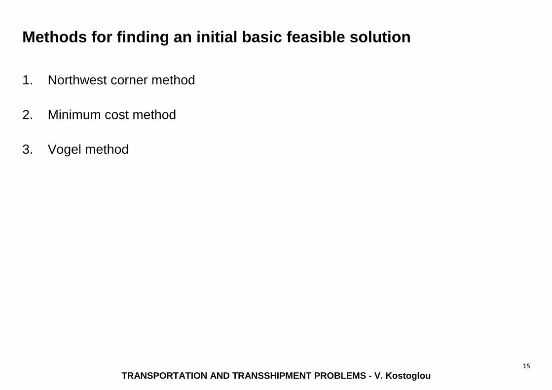
Methods for finding an initial basic feasible solution
1. Northwest corner method
2. Minimum cost method
3. Vogel method
16
TRANSPORTATION AND TRANSSHIPMENT PROBLEMS - V. Kostoglou
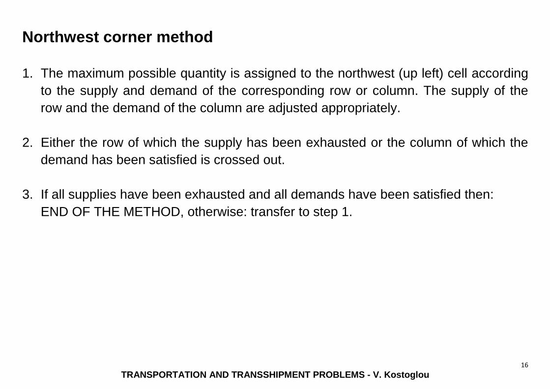
Northwest corner method
1. The maximum possible quantity is assigned to the northwest (up left) cell according
to the supply and demand of the corresponding row or column. The supply of the
row and the demand of the column are adjusted appropriately.
2. Either the row of which the supply has been exhausted or the column of which the
demand has been satisfied is crossed out.
3. If all supplies have been exhausted and all demands have been satisfied then:
END OF THE METHOD, otherwise: transfer to step 1.
17
TRANSPORTATION AND TRANSSHIPMENT PROBLEMS - V. Kostoglou
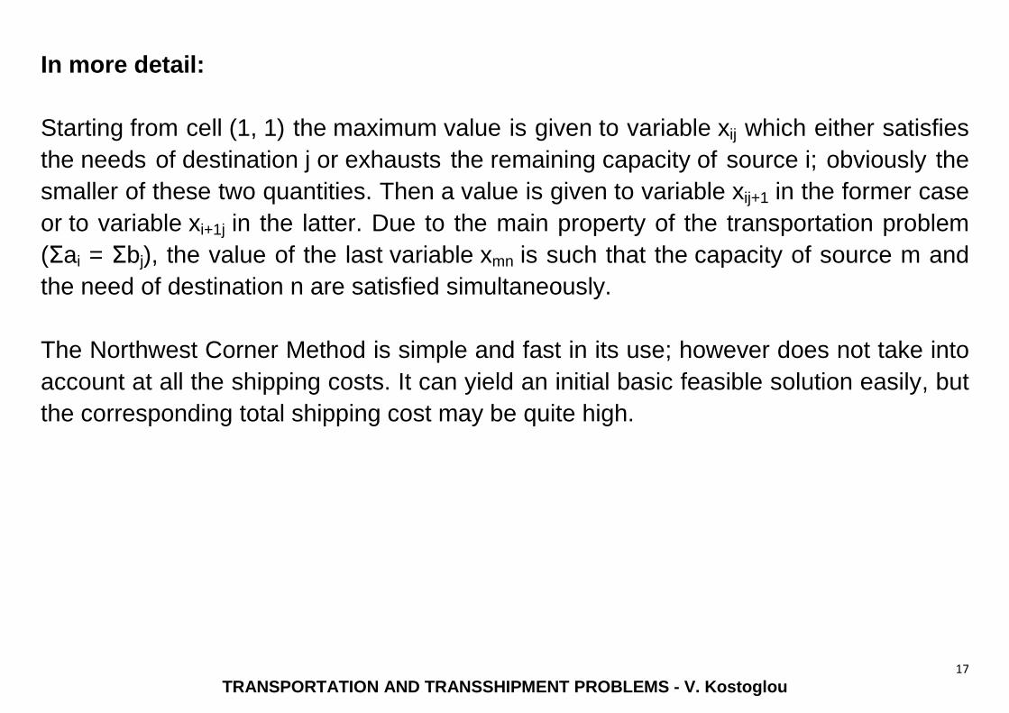
In more detail:
Starting from cell (1, 1) the maximum value is given to variable xij which either satisfies
the needs of destination j or exhausts the remaining capacity of source i; obviously the
smaller of these two quantities. Then a value is given to variable xij+1 in the former case
or to variable xi+1j in the latter. Due to the main property of the transportation problem
(Σai = Σbj), the value of the last variable xmn is such that the capacity of source m and
the need of destination n are satisfied simultaneously.
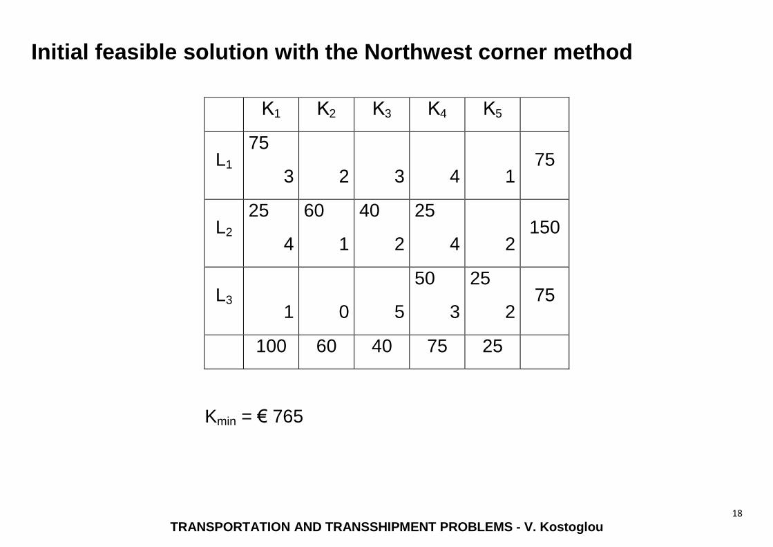
The Northwest Corner Method is simple and fast in its use; however does not take into
account at all the shipping costs. It can yield an initial basic feasible solution easily, but
the corresponding total shipping cost may be quite high.
18
TRANSPORTATION AND TRANSSHIPMENT PROBLEMS - V. Kostoglou
Initial feasible solution with the Northwest corner method
Κ1 Κ2 Κ3 Κ4 Κ5
L1 75
3
2
3
4
1 75
L2 25
4
60
1
40
2
25
4
2 150
L3
1
0
5
50
3
25
2 75
100 60 40 75 25
Kmin = € 765
19
TRANSPORTATION AND TRANSSHIPMENT PROBLEMS - V. Kostoglou
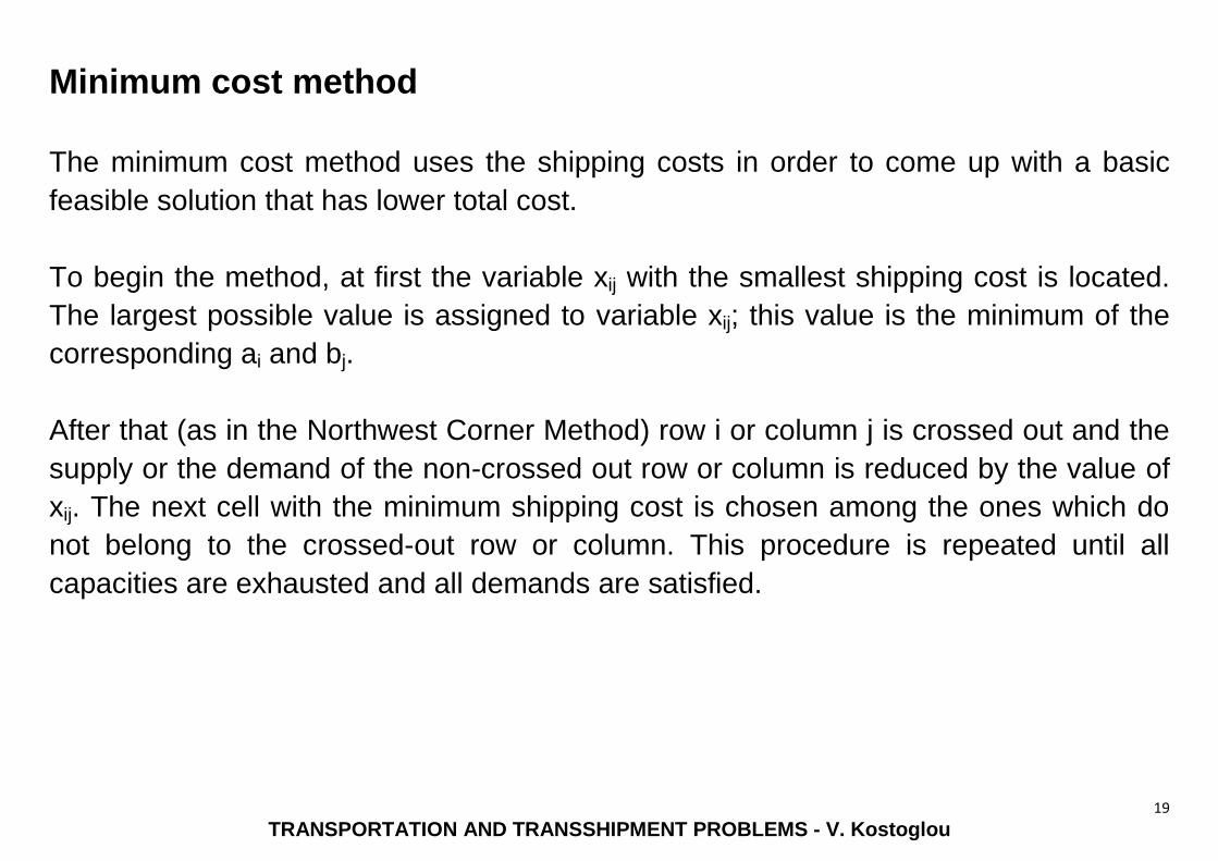
Minimum cost method
The minimum cost method uses the shipping costs in order to come up with a basic
feasible solution that has lower total cost.
To begin the method, at first the variable xij with the smallest shipping cost is located.
The largest possible value is assigned to variable xij; this value is the minimum of the
corresponding ai and bj.
After that (as in the Northwest Corner Method) row i or column j is crossed out and the
supply or the demand of the non-crossed out row or column is reduced by the value of
xij. The next cell with the minimum shipping cost is chosen among the ones which do
not belong to the crossed-out row or column. This procedure is repeated until all
capacities are exhausted and all demands are satisfied.
20
TRANSPORTATION AND TRANSSHIPMENT PROBLEMS - V. Kostoglou
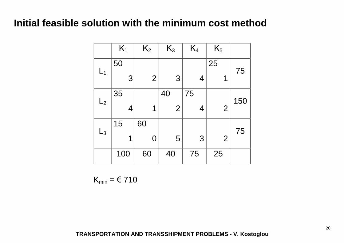
Initial feasible solution with the minimum cost method
Κ1 Κ2 Κ3 Κ4 Κ5
L1 50
3
2
3
4
25
1 75
L2 35
4
1
40
2
75
4
2 150
L3 15
1
60
0
5
3
2 75
100 60 40 75 25
Kmin = € 710
21
TRANSPORTATION AND TRANSSHIPMENT PROBLEMS - V. Kostoglou
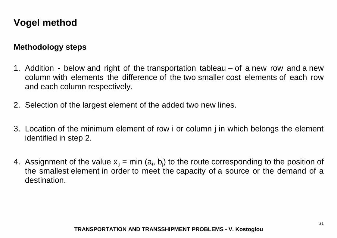
Vogel method
Methodology steps
1. Addition - below and right of the transportation tableau – of a new row and a new column with elements the difference of the two smaller cost elements of each row and each column respectively.
2. Selection of the largest element of the added two new lines.
3. Location of the minimum element of row i or column j in which belongs the element identified in step 2.
4. Assignment of the value xij = min (ai, bj) to the route corresponding to the position of the smallest element in order to meet the capacity of a source or the demand of a destination.
22
TRANSPORTATION AND TRANSSHIPMENT PROBLEMS - V. Kostoglou
5. If the capacity of a source is exhausted, then the demand bj of the corresponding destination is reduced by ai. In contrary, if the demand of a destination is satisfied, then the capacity ai of the corresponding source is reduced by bj. The source (row) or destination (column) that was satisfied is crossed-out and is not taken further into account.
Each time the above procedure is repeated the capacity of a source is exhausted or the
needs of a destination are satisfied. The implementation of the method is completed
when the capacity of the last row and the needs of the last column are simultaneously
satisfied. The solution yielded is feasible because it meets all capacities and all needs.
23
TRANSPORTATION AND TRANSSHIPMENT PROBLEMS - V. Kostoglou
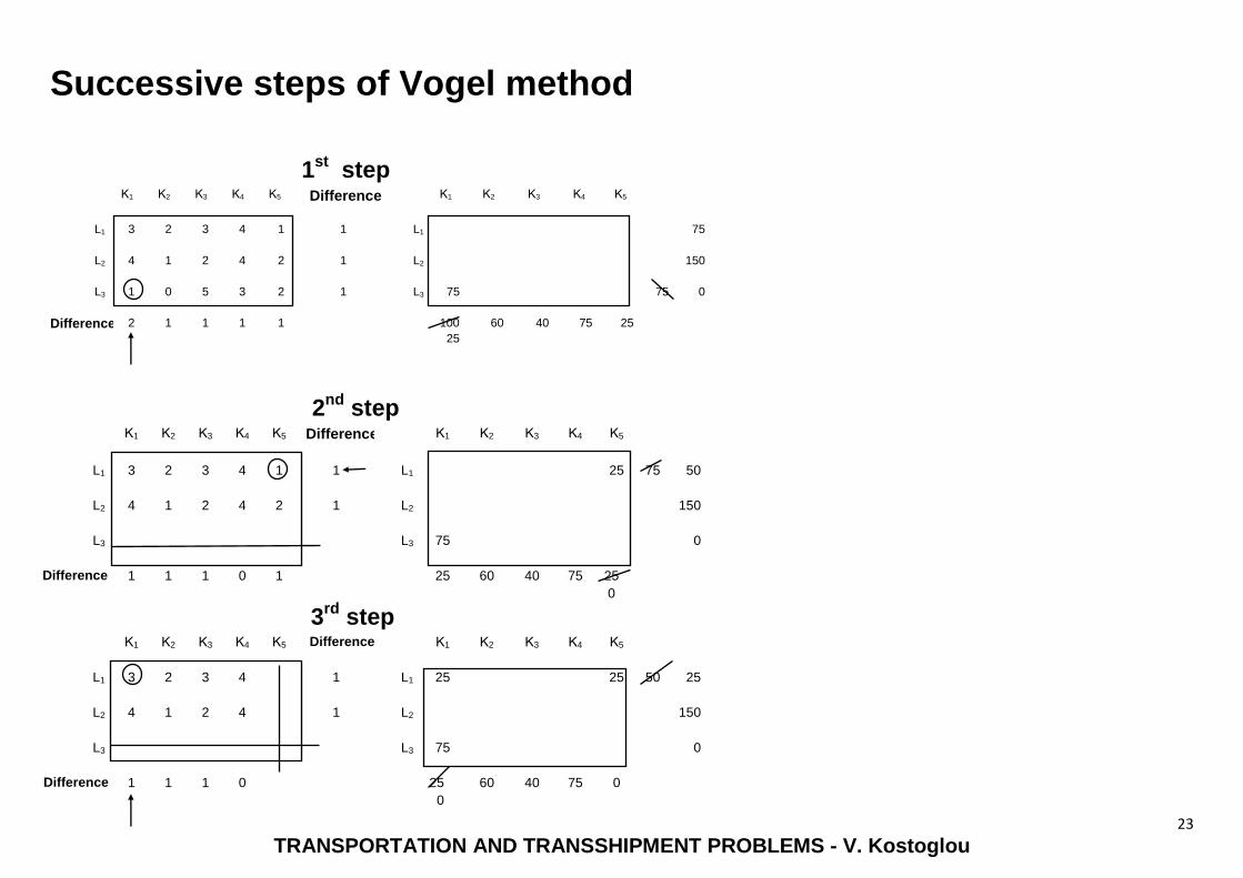
Successive steps of Vogel method
1
st step
Κ1 Κ2 Κ3 Κ4 Κ5 Difference Κ1 Κ2 Κ3 Κ4 Κ5
L1 3 2 3 4 1 1 L1 75
L2 4 1 2 4 2 1 L2 150
L3 1 0 5 3 2 1 L3 75 75 0
Difference 2 1 1 1 1 100
25
60 40 75 25
2
nd step
Κ1 Κ2 Κ3 Κ4 Κ5 Differencee Κ1 Κ2 Κ3 Κ4 Κ5
L1 3 2 3 4 1 1 L1 25 75 50
L2 4 1 2 4 2 1 L2 150
L3 L3 75 0
DDifference 1 1 1 0 1 25
60 40 75 25
0
3rd
step Κ1 Κ2 Κ3 Κ4 Κ5 Difference Κ1 Κ2 Κ3 Κ4 Κ5
L1 3 2 3 4 1 L1 25 25 50 25
L2 4 1 2 4 1 L2 150
L3 L3 75 0
Difference 1 1 1 0 25
0
60 40 75 0
24
TRANSPORTATION AND TRANSSHIPMENT PROBLEMS - V. Kostoglou
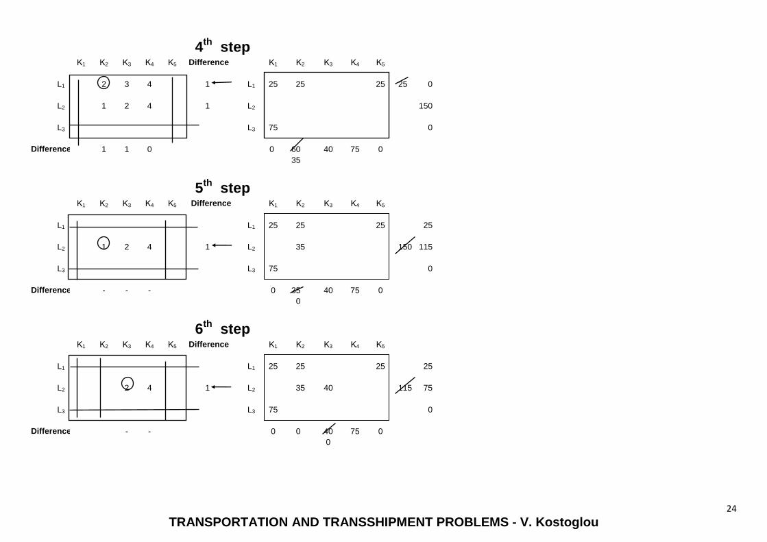
4th
step Κ1 Κ2 Κ3 Κ4 Κ5 Difference Κ1 Κ2 Κ3 Κ4 Κ5
L1 2 3 4 1 L1 25 25 25 25 0
L2 1 2 4 1 L2 150
L3 L3 75 0
Difference 1 1 0 0
60
35
40 75 0
5th
step Κ1 Κ2 Κ3 Κ4 Κ5 Difference Κ1 Κ2 Κ3 Κ4 Κ5
L1 L1 25 25 25 25
L2 1 2 4 1 L2 35 150 115
L3 L3 75 0
Difference - - - 0 35
0
40 75 0
6th
step Κ1 Κ2 Κ3 Κ4 Κ5 Difference Κ1 Κ2 Κ3 Κ4 Κ5
L1 L1 25 25 25 25
L2 2 4 1 L2 35 40 115 75
L3 L3 75 0
Difference - - 0 0
40
0
75 0
25
TRANSPORTATION AND TRANSSHIPMENT PROBLEMS - V. Kostoglou
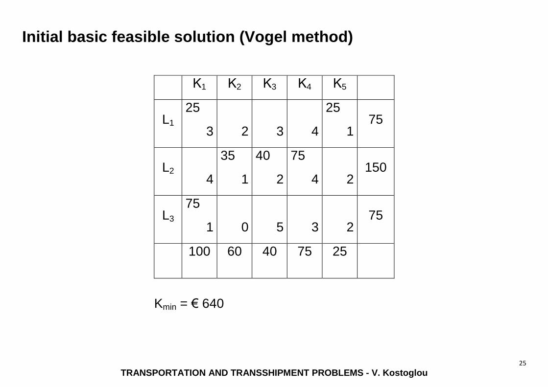
Initial basic feasible solution (Vogel method)
Κ1 Κ2 Κ3 Κ4 Κ5
L1 25
3
2
3
4
25
1 75
L2
4
35
1
40
2
75
4
2 150
L3 75
1
0
5
3
2 75
100 60 40 75 25
Kmin = € 640
26
TRANSPORTATION AND TRANSSHIPMENT PROBLEMS - V. Kostoglou
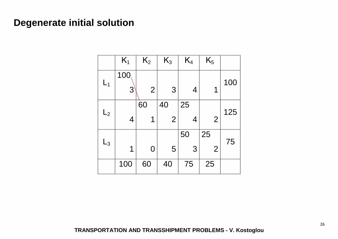
Degenerate initial solution
Κ1 Κ2 Κ3 Κ4 Κ5
L1 100
3
2
3
4
1 100
L2
4
60
1
40
2
25
4
2 125
L3
1
0
5
50
3
25
2 75
100 60 40 75 25
27
TRANSPORTATION AND TRANSSHIPMENT PROBLEMS - V. Kostoglou
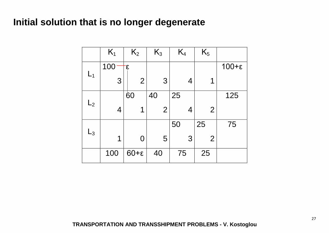
Initial solution that is no longer degenerate
Κ1 Κ2 Κ3 Κ4 Κ5
L1 100
3
ε
2
3
4
1
100+ε
L2
4
60
1
40
2
25
4
2
125
L3
1
0
5
50
3
25
2
75
100 60+ε 40 75 25
28
TRANSPORTATION AND TRANSSHIPMENT PROBLEMS - V. Kostoglou
Transportation problems solution methodology
Initial step
Creation of an initial basic feasible solution using one of the three relevant methods.
Transfer to the termination rule.
Repeating step
1. Determination of the incoming variable that will be introduced to the base:
Selection of the non basic variable xij with maximum negative difference cij - ui - vj
2. Determination of the outgoing variable that will be removed from the base:
Identification of the (unique) loop, which’s all vertices are basic variables.
Assignment of the maximum possible value to the incoming variable.
For its determination is selected among the donor routes the one with the
smallest value. The corresponding variable is removed from the basis.
29
TRANSPORTATION AND TRANSSHIPMENT PROBLEMS - V. Kostoglou
3. Determination of the new basic feasible solution:
Addition of the quantity θ to each recipient route and deduction from each donor
route, so that all constraints of sources and destinations are met.
Termination rule
Calculation of the elements ui and vj.
[It is suggested to select the line (row or column) with the largest number of basic
variables, giving to the corresponding ui (vj) the zero value and solving the simple
system of equations cij = ui + vj for each basic route (i, j)]
Solution optimality control
If for each non basic route (i,j) ui + vj <= cij then the solution is optimal End.
In not, go to the repetitive step.

30
TRANSPORTATION AND TRANSSHIPMENT PROBLEMS - V. Kostoglou
Successive steps of finding the optimal solution
1st
repetition
Κ1 Κ2 Κ3 Κ4 Κ5
vj
ui
4 1 2 4 3
L1
-1
75
3
2
3
4
*
1
75
L2
-0
25-θ
4
60
1
40
2
25+θ
4
*
2
150
L3
-1
θ *
1
0
5
50-θ
3
25
2
75
100 60 40 75 25

31
TRANSPORTATION AND TRANSSHIPMENT PROBLEMS - V. Kostoglou
The largest quantity that can be transferred from route L2 - Κ1 (outgoing variable) to
the route L3 - Κ1 (incoming variable as c31 = u3 - v1 = 1-(-1)-4 = -2 < 0) is θmax = 25.
2nd
repetition
Κ1 Κ2 Κ3 Κ4 Κ5
vj
ui
2 1 2 4 3
L1
1
75-θ
3
2
3
*
4
θ *
1
75
L2
-0
4
60
1
40
2
50
4
*
2
150
L3
-1
25+θ
1
0
5
25
3
25-θ
2
75
100 60 40 75 25
32
TRANSPORTATION AND TRANSSHIPMENT PROBLEMS - V. Kostoglou
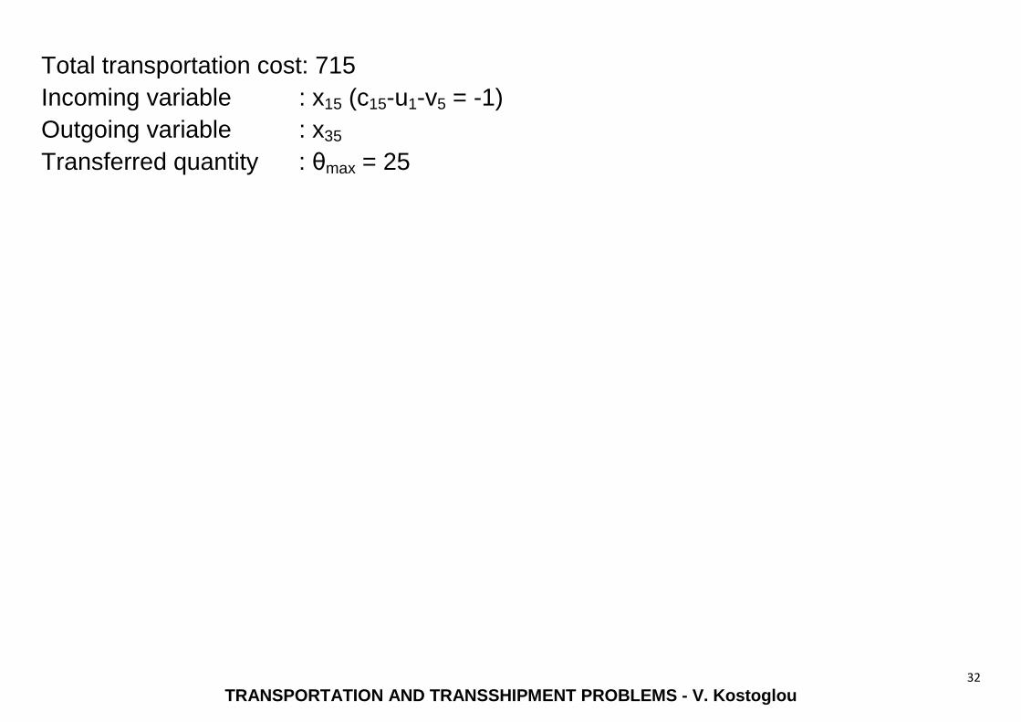
Total transportation cost: 715
Incoming variable : x15 (c15-u1-v5 = -1)
Outgoing variable : x35
Transferred quantity : θmax = 25
33
TRANSPORTATION AND TRANSSHIPMENT PROBLEMS - V. Kostoglou
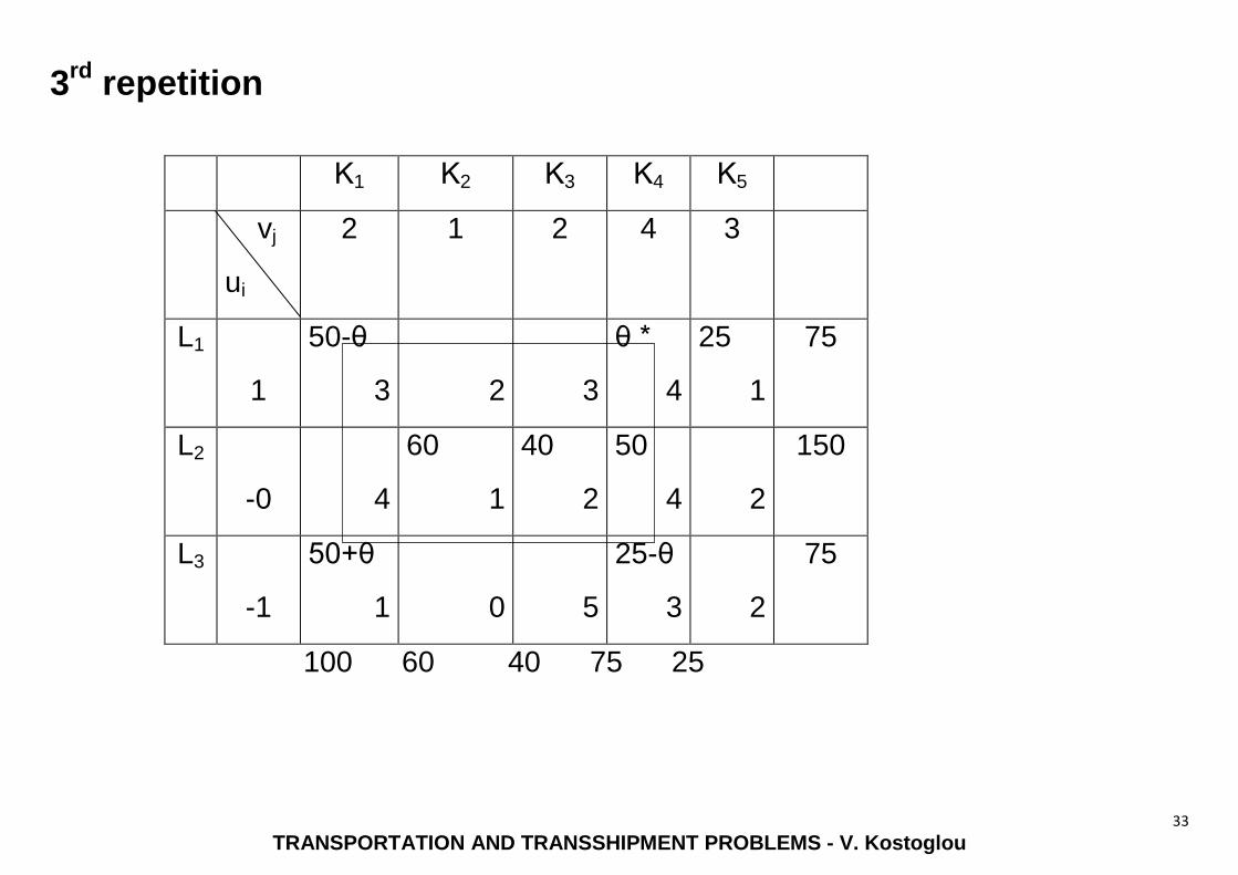
3rd
repetition
Κ1 Κ2 Κ3 Κ4 Κ5
vj
ui
2 1 2 4 3
L1
1
50-θ
3
2
3
θ *
4
25
1
75
L2
-0
4
60
1
40
2
50
4
2
150
L3
-1
50+θ
1
0
5
25-θ
3
2
75
100 60 40 75 25
34
TRANSPORTATION AND TRANSSHIPMENT PROBLEMS - V. Kostoglou
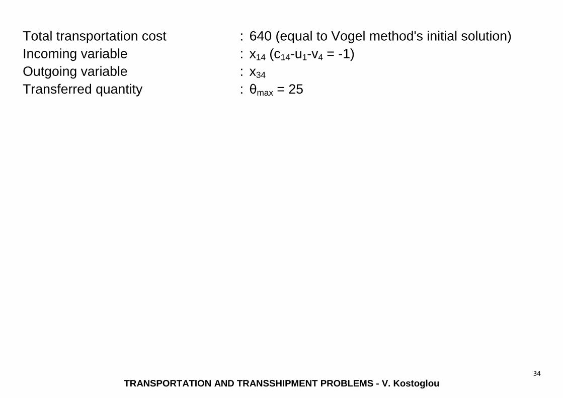
Total transportation cost : 640 (equal to Vogel method's initial solution)
Incoming variable : x14 (c14-u1-v4 = -1)
Outgoing variable : x34
Transferred quantity : θmax = 25

35
TRANSPORTATION AND TRANSSHIPMENT PROBLEMS - V. Kostoglou
4th
repetition
Κ1 Κ2 Κ3 Κ4 Κ5
vj
ui
2 1 2 4 3
L1
1
25
3
2
3
25
4
25
1
75
L2
-0
4
60
1
40
2
50
4
2
150
L3
-1
75
1
0
5
3
2
75
100 60 40 75 25
36
TRANSPORTATION AND TRANSSHIPMENT PROBLEMS - V. Kostoglou
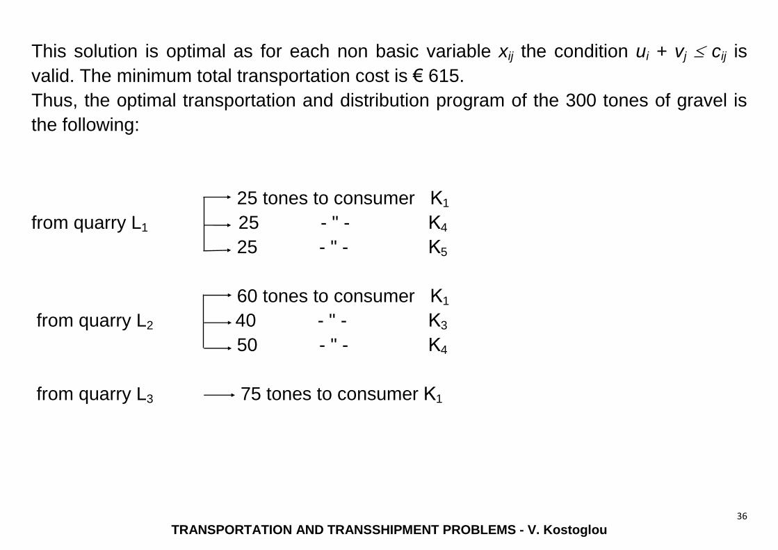
This solution is optimal as for each non basic variable xij the condition ui + vj cij is
valid. The minimum total transportation cost is € 615.
Thus, the optimal transportation and distribution program of the 300 tones of gravel is
the following:
25 tones to consumer Κ1
from quarry L1 25 - " - Κ4
25 - " - Κ5
60 tones to consumer Κ1
from quarry L2 40 - " - Κ3
50 - " - Κ4
from quarry L3 75 tones to consumer Κ1
37
TRANSPORTATION AND TRANSSHIPMENT PROBLEMS - V. Kostoglou
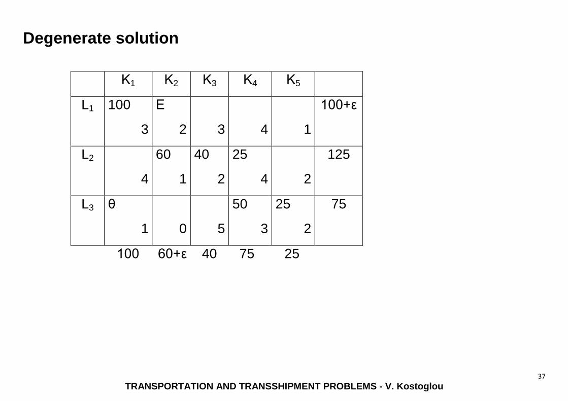
Degenerate solution
Κ1 Κ2 Κ3 Κ4 Κ5
L1
100
3
Ε
2
3
4
1
100+ε
L2
4
60
1
40
2
25
4
2
125
L3
θ
1
0
5
50
3
25
2
75
100 60+ε 40 75 25

38
TRANSPORTATION AND TRANSSHIPMENT PROBLEMS - V. Kostoglou
1st
repetition
Κ1 Κ2 Κ3 Κ4 Κ5
vj
ui
2 1 2 4 3
L1
1
100
3
ε-θ
2
3
*
4
θ*
1
100+ε
L2
0
4
60-θ
1
40
2
25-θ
4
*
2
125
L3
-1
1
0
5
50-θ
3
25-θ
2
75
100 60+ε 40 75 25
With asterisk (*) are marked all the routes with negative difference cij-ui-vj
39
TRANSPORTATION AND TRANSSHIPMENT PROBLEMS - V. Kostoglou
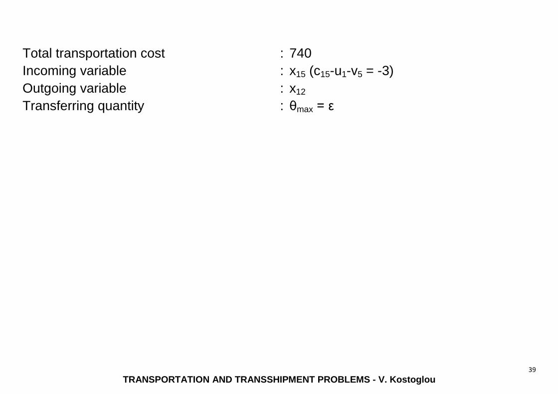
Total transportation cost
:
740
Incoming variable : x15 (c15-u1-v5 = -3)
Outgoing variable : x12
Transferring quantity : θmax = ε
40
TRANSPORTATION AND TRANSSHIPMENT PROBLEMS - V. Kostoglou
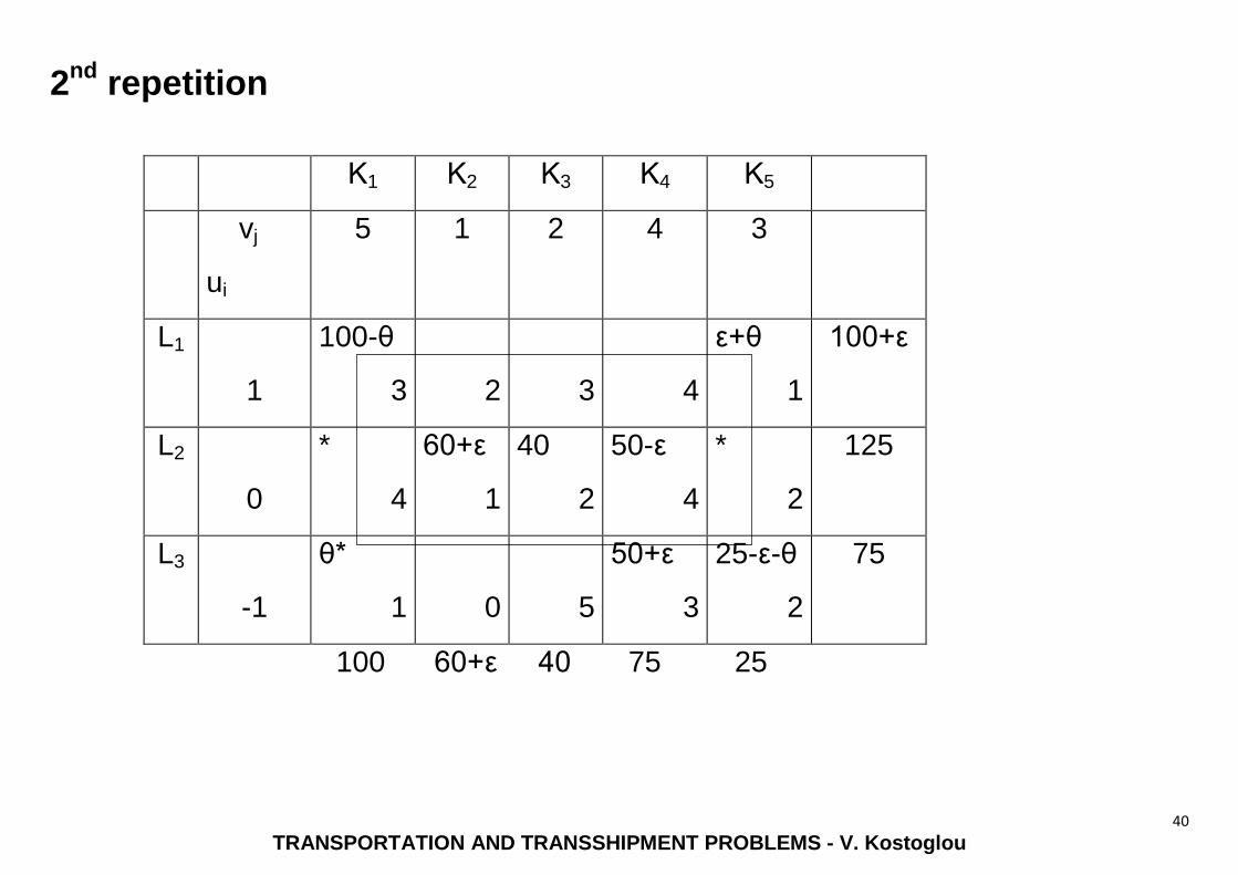
2nd
repetition
Κ1 Κ2 Κ3 Κ4 Κ5
vj
ui
5 1 2 4 3
L1
1
100-θ
3
2
3
4
ε+θ
1
100+ε
L2
0
*
4
60+ε
1
40
2
50-ε
4
*
2
125
L3
-1
θ*
1
0
5
50+ε
3
25-ε-θ
2
75
100 60+ε 40 75 25
41
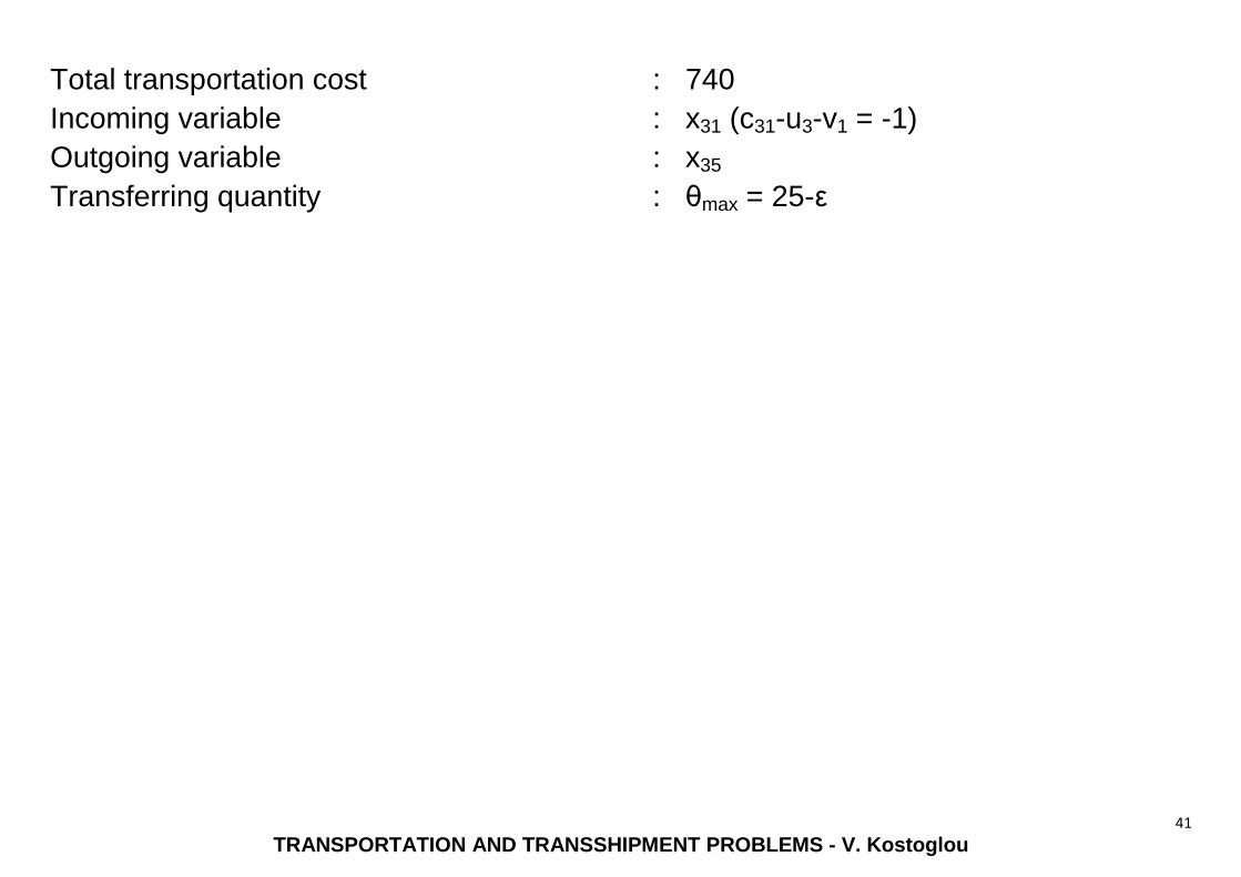
TRANSPORTATION AND TRANSSHIPMENT PROBLEMS - V. Kostoglou
Total transportation cost : 740
Incoming variable : x31 (c31-u3-v1 = -1)
Outgoing variable : x35
Transferring quantity
: θmax = 25-ε
42
TRANSPORTATION AND TRANSSHIPMENT PROBLEMS - V. Kostoglou
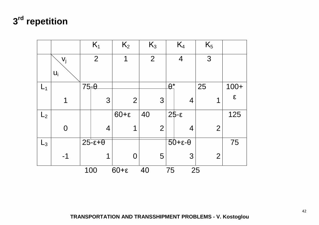
3rd
repetition
Κ1 Κ2 Κ3 Κ4 Κ5
vj
ui
2 1 2 4 3
L1
1
75-θ
3
2
3
θ*
4
25
1
100+
ε
L2
0
4
60+ε
1
40
2
25-ε
4
2
125
L3
-1
25-ε+θ
1
0
5
50+ε-θ
3
2
75
100 60+ε 40 75 25
43
TRANSPORTATION AND TRANSSHIPMENT PROBLEMS - V. Kostoglou
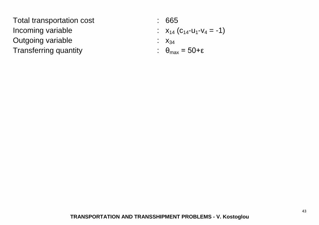
Total transportation cost : 665
Incoming variable : x14 (c14-u1-v4 = -1)
Outgoing variable : x34
Transferring quantity
: θmax = 50+ε
44
TRANSPORTATION AND TRANSSHIPMENT PROBLEMS - V. Kostoglou
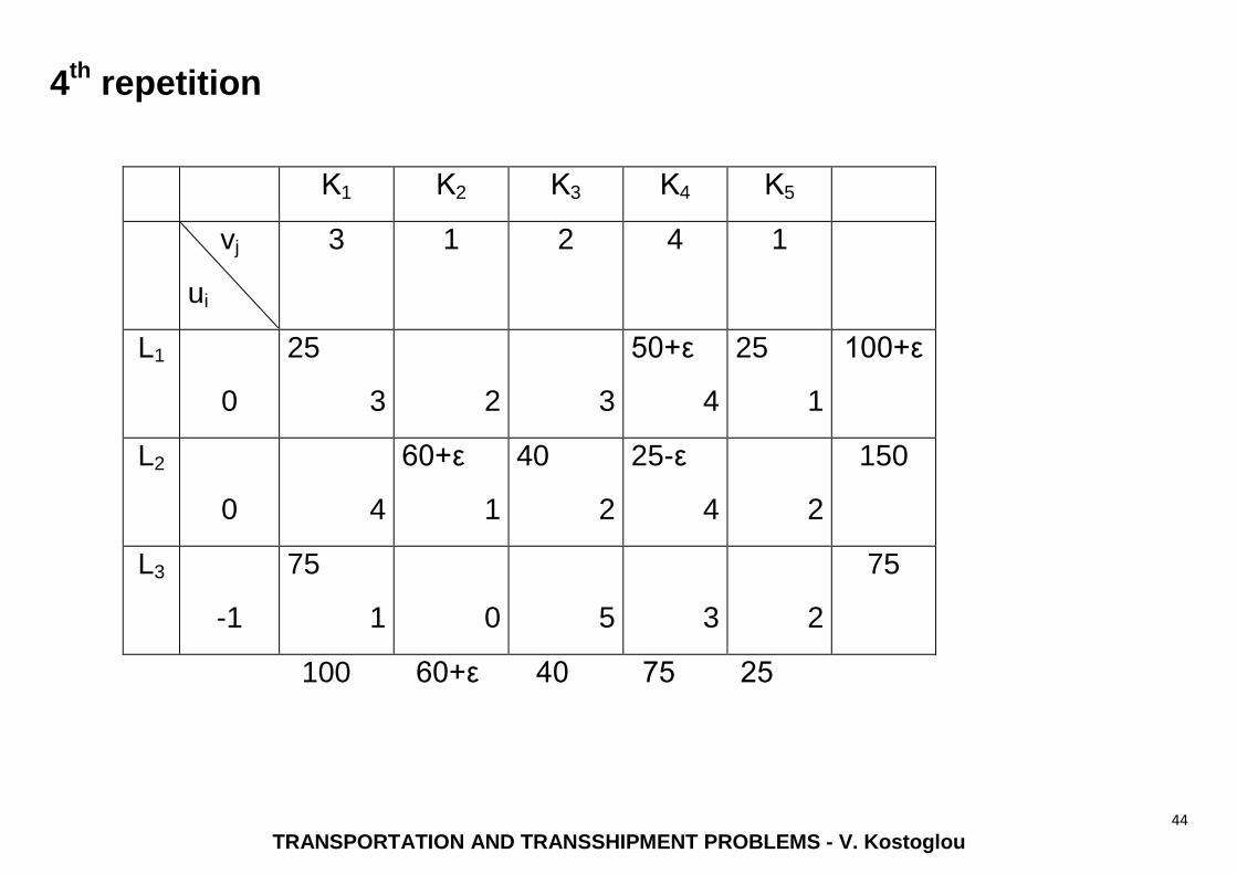
4th
repetition
Κ1 Κ2 Κ3 Κ4 Κ5
vj
ui
3 1 2 4 1
L1
0
25
3
2
3
50+ε
4
25
1
100+ε
L2
0
4
60+ε
1
40
2
25-ε
4
2
150
L3
-1
75
1
0
5
3
2
75
100 60+ε 40 75 25
45
TRANSPORTATION AND TRANSSHIPMENT PROBLEMS - V. Kostoglou
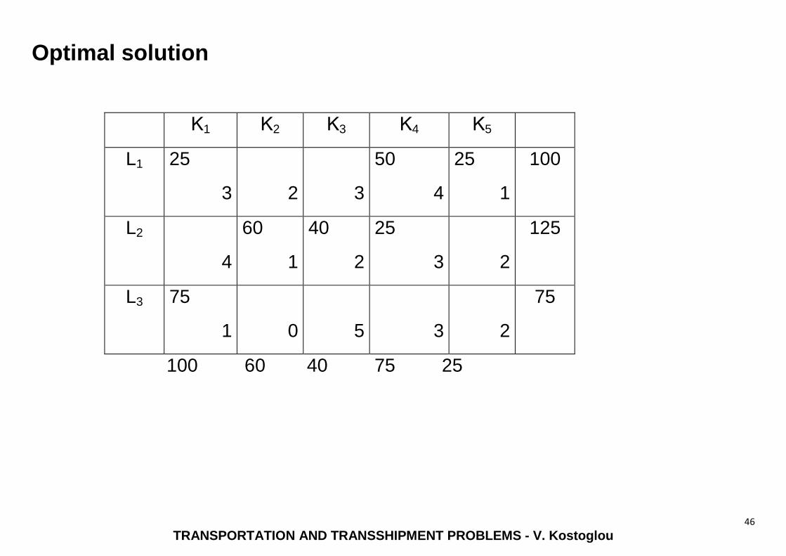
For all non basic routes of the last table the condition ui + vj cij is valid, so the current
solution is optimal. In order to identify this solution the auxiliary variable ε is deleted,
having completed its contribution.
The total transportation cost (€ 615) and the analytical program of transportation and
distribution of 300 tones of gravel can now be determined.
46
TRANSPORTATION AND TRANSSHIPMENT PROBLEMS - V. Kostoglou
Optimal solution
Κ1 Κ2 Κ3 Κ4 Κ5
L1
25
3
2
3
50
4
25
1
100
L2
4
60
1
40
2
25
3
2
125
L3
75
1
0
5
3
2
75
100 60 40 75 25
47
TRANSPORTATION AND TRANSSHIPMENT PROBLEMS - V. Kostoglou
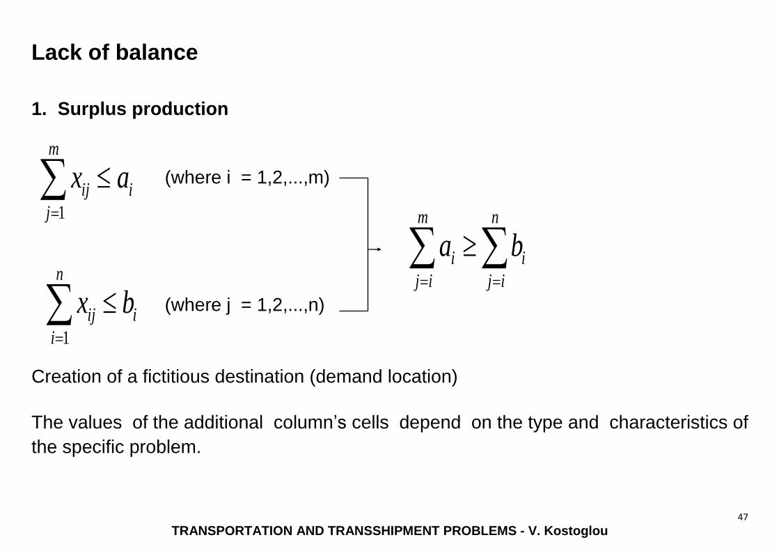
Lack of balance
1. Surplus production
(where i = 1,2,...,m)
(where j = 1,2,...,n)
Creation of a fictitious destination (demand location)
The values of the additional column’s cells depend on the type and characteristics of
the specific problem.
i
m
j
ij ax 1
i
n
i
ij bx 1
n
ij
i
m
ij
i ba
48
TRANSPORTATION AND TRANSSHIPMENT PROBLEMS - V. Kostoglou
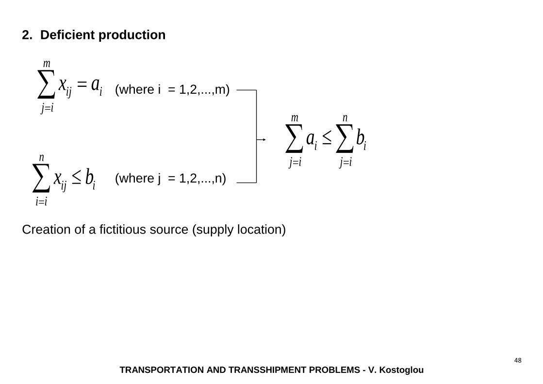
2. Deficient production
(where i = 1,2,...,m)
(where j = 1,2,...,n)
Creation of a fictitious source (supply location)
i
n
ii
ij bx
n
ij
i
m
ij
i ba
i
m
ij
ij ax

49
TRANSPORTATION AND TRANSSHIPMENT PROBLEMS - V. Kostoglou
Regarding the elements of the additional row:
If the shortage cost of a quantity that has to be transported to a destination is zero,
the corresponding cost element is equal to zero.
If the inability to meet the demand implies some economic consequences
(penalties, discounts, cost of good reputation, etc), then the cost of each cell
of the additional row is put equal to the corresponding unit shortage cost.
50
TRANSPORTATION AND TRANSSHIPMENT PROBLEMS - V. Kostoglou
3. Satisfaction obligation
In these cases the transportation tableau has to be formed in such a way that
the corresponding additional route of the fictitious source or destination will not
participate in any case in the final solution.
For this purpose, a very large positive value (M) is given to the cost element of this
route. This ensures that this route will not participate in any case in the final solution.
51
TRANSPORTATION AND TRANSSHIPMENT PROBLEMS - V. Kostoglou
4. Surplus or deficient production
It is possible that in some transportation problems it is not known in advance whether
the production will be surplus or deficient. This can happen if the elements cij of the
objective function represent results (profit, loss or another efficiency criterion) from the
satisfaction of a demand location. Some of these elements may be negative. Therefore,
it may be preferable not to satisfy at all a demand if the corresponding economic results
to a loss.
In order to address such a situation a fictitious source (row) and a fictitious destination
(column) are added to the initial transportation table. The capacity and demand of the
two additional lines should be such as neither the satisfaction of all demands or the
exhaustion of all capacities is compulsory.
52
TRANSPORTATION AND TRANSSHIPMENT PROBLEMS - V. Kostoglou
Solution of maximization problems
In such a case the target is the maximization of the objective function. The
methodology of finding the optimal solution of such a problem is nearly identical to that
of minimization problems. The successive steps after the determination of an initial
feasible solution remain unchanged. The only difference refers to the termination
rule examining the optimality of the solution:
The current solution is optimal if for any non-basic route is valid: ui + vj cij

53
TRANSPORTATION AND TRANSSHIPMENT PROBLEMS - V. Kostoglou
Differences in the methods of finding an initial solution
Northwest corner method: No difference.
Minimum cost method: In practice it is renamed to “maximum profit method”.
So, keeping the same logic, the priority is the assignment of the maximum possible
quantity to the route with the highest unit profit.
Vogel method: The differences, due to its complexity, are more:
- Step 1: The elements of the additional column and row are the differences
between the two larger profit elements of each row and column respectively.
- Step 3: The largest element of the appropriate column or row is searched out in
the transportation table.
.
54
TRANSPORTATION AND TRANSSHIPMENT PROBLEMS - V. Kostoglou
TRANSSHIPMENT PROBLEMS
One of the main requirements of the transportation problems is the a priori knowledge
of the way the units will be transported from every source i to every destination j, and
the corresponding unit cost cij can be determined.
Nevertheless, sometimes the best way of transportation is not clear due to the
possibility of transshipments. In this case the products are sent through intermediate
transfer points (that can also be other sources or destinations). Such cases should be
examined from scratch in order to identify the most economical route from each source
to each destination. If there are many possible intermediate transfer points, the
determination of this cheapest route can become extremely complex and time
consuming.
For this purpose a special algorithm determining the transferred quantities for each
source to each destination, as well as the route that will follow each load in order to
minimize the total shipping cost.
55
TRANSPORTATION AND TRANSSHIPMENT PROBLEMS - V. Kostoglou
The extension of the transportation problem that includes the decisions about the
intermediate routings is called transshipment problem.
A simple way of transshipment problem formulation has been developed so that it can
be adapted to the transportation problem standard model. So, the Simplex method
used for transportation problems can also be used for solving transshipment problems.
56
TRANSPORTATION AND TRANSSHIPMENT PROBLEMS - V. Kostoglou
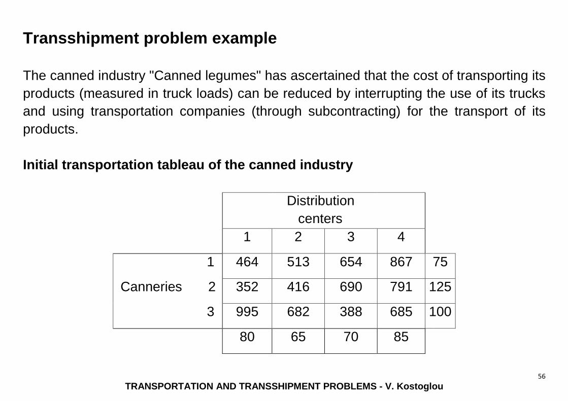
Transshipment problem example
The canned industry "Canned legumes" has ascertained that the cost of transporting its
products (measured in truck loads) can be reduced by interrupting the use of its trucks
and using transportation companies (through subcontracting) for the transport of its
products.
Initial transportation tableau of the canned industry
Distribution
centers
1 2 3 4
1 464 513 654 867 75
Canneries 2 352 416 690 791 125
3 995 682 388 685 100
80 65 70 85

57
TRANSPORTATION AND TRANSSHIPMENT PROBLEMS - V. Kostoglou
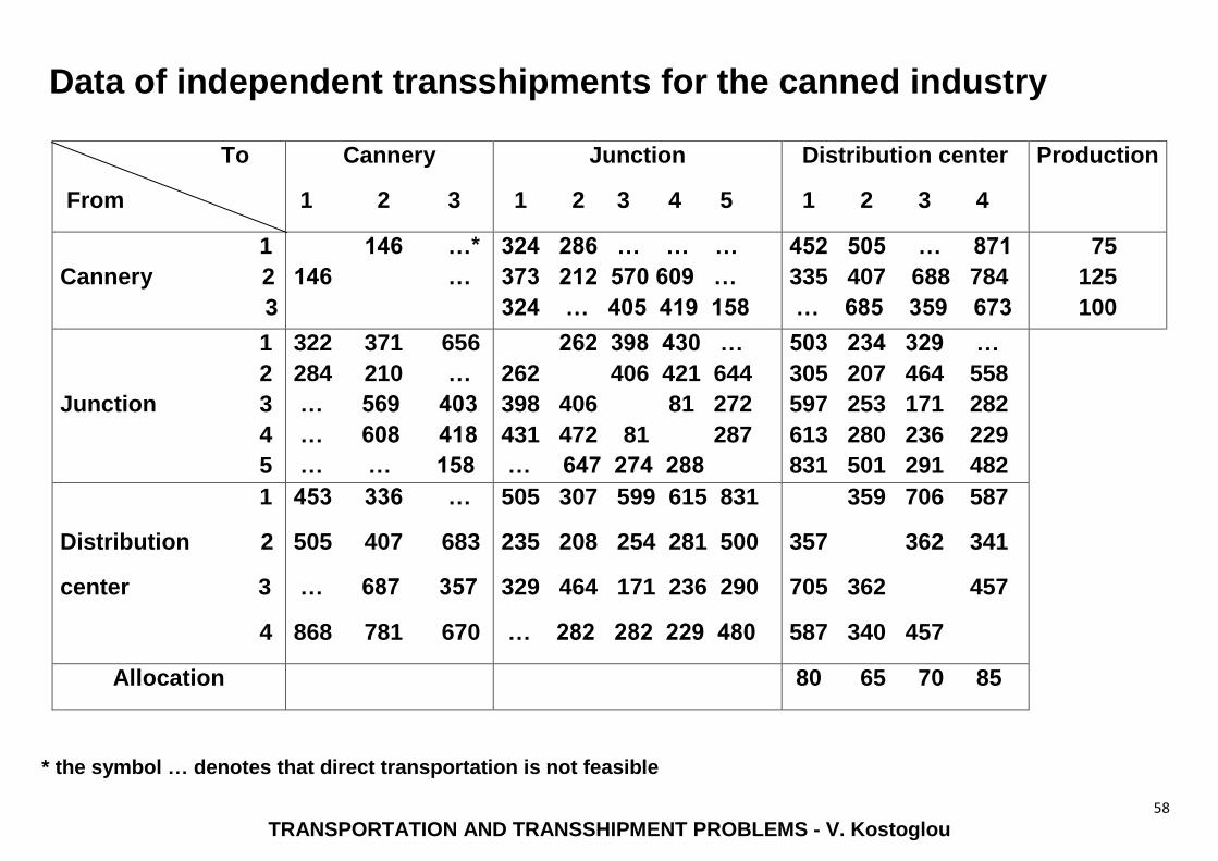
As there is no transportation company that can service the whole region containing
company's canneries and distribution centers, some loads need at least once during
their route from source to final destination to get transshipped to another truck. These
transshipments can be carried out to intermediate canneries or distribution centers od
to five other locations called junctions.
The transportation cost per load among canneries, distribution centers and junctions is
presented in the following summary table.
58
TRANSPORTATION AND TRANSSHIPMENT PROBLEMS - V. Kostoglou
Data of independent transshipments for the canned industry To
From
Cannery
1 2 3
Junction
1 2 3 4 5
Distribution center
1 2 3 4
Production
1
Cannery 2
3
146 …*
146 …
324 286 … … …
373 212 570 609 …
324 … 405 419 158
452 505 … 871
335 407 688 784
… 685 359 673
75
125
100
1
2
Junction 3
4
5
322 371 656
284 210 …
… 569 403
… 608 418
… … 158
262 398 430 …
262 406 421 644
398 406 81 272
431 472 81 287
… 647 274 288
503 234 329 …
305 207 464 558
597 253 171 282
613 280 236 229
831 501 291 482
1
Distribution 2
center 3
4
453 336 …
505 407 683
… 687 357
868 781 670
505 307 599 615 831
235 208 254 281 500
329 464 171 236 290
… 282 282 229 480
359 706 587
357 362 341
705 362 457
587 340 457
Allocation 80 65 70 85
* the symbol … denotes that direct transportation is not feasible
59
TRANSPORTATION AND TRANSSHIPMENT PROBLEMS - V. Kostoglou
The most effective approach for reaching the solution of transshipment problem is its
reformulation as a transportation problem, so that it can be solved with the already
known method. The basic idea for this purpose is the consideration of each movement
of a truck as transportation form a source to a destination. Therefore all locations
(canneries, junctions and distribution centers) are considered as both; possible sources
and possible destinations for all transportations..
Thus it is considered that there are 12 sources (3 canneries + 4 distribution centers + 5
junctions) and 12 destinations. The corresponding transportation costs cij (where i = 1,
2, … 12 και j = 1, 2, … 12) are given in the following table. The big Μ (Μ >> 0) is used
for the non feasible transportations (that were denoted with ... in the previous table).

60
TRANSPORTATION AND TRANSSHIPMENT PROBLEMS - V. Kostoglou
The number of loads that are transshipped through each location has to be included to
both; the needs of this location as destination and the supply of this location as source.
As this number is not known in advance, an upper limit has to be added in the demand
and the supply of the location. Then a dummy variable has to be inserted in the
demand and supply constraints, in order to allocate this surplus amount. As it is not
economically efficient to transship a load to the same location more than once, a safe
upper limit for any location is the total number of the 300 produced loads.
The final cost table with the corresponding supplies and demands can now be compiled
as a transportation problem model of this transshipment problem.

61
TRANSPORTATION AND TRANSSHIPMENT PROBLEMS - V. Kostoglou
Costs table of the transshipment problem transformed as
transportation problem
Destination
Source
Canneries
1 2 3
Junctions
1 2 3 4 5
Distribution centers
1 2 3 4
Supply
1
Canneries 2
3
0 146 Μ
146 0 Μ
Μ Μ 0
324 286 Μ Μ Μ
373 212 570 609 Μ
658 Μ 405 419 158
452 505 Μ 871
335 407 688 784
Μ 685 359 673
375
425
400
1
2
Junctions 3
4
5
322 371 656
284 210 Μ
Μ 569 403
Μ 608 418
Μ Μ 158
0 262 398 430 Μ
262 0 406 421 644
398 406 0 81 272
431 472 81 0 287
Μ 647 274 288 0
503 234 329 Μ
305 207 464 558
597 253 171 282
613 280 236 229
831 501 291 482
300
300
300
300
300
1
Distribution 2
3
4
453 336 Μ
505 407 683
Μ 687 357
868 781 670
505 307 599 615 831
235 208 254 281 500
329 464 171 236 290
Μ 282 282 229 480
0 359 706 587
357 0 362 341
705 362 0 457
587 340 457 0
300
300
300
300
Demand 300 300 300 300 300 300 300 300 80 65 70 85
62
TRANSPORTATION AND TRANSSHIPMENT PROBLEMS - V. Kostoglou
The optimal solution of the transshipment problem of the canned industry "Canned
legumes" can now be determined with the use of the Simplex method of transportation
problems. Due to the relatively large size of the problem (m=n=12) the use of software
is essential.