Transmission Effects in the Presence of Structural Breaks...

1

Transmission Effects in the Presence of Structural

Breaks: Evidence from South-Eastern European

Countries

Minoas Koukouritakis

Department of Economics, University of Crete, Greece

Athanasios P. Papadopoulos*


Andreas Yannopoulos


Abstract: In this paper, we investigate the monetary transmission mechanism through interest

rate and real effective exchange rate channels, for five South-Eastern European countries,

namely Bulgaria, Croatia, Greece, Romania and Turkey. Recent unit root and cointegration

techniques in the presence of structural breaks in the data have been used in the analysis. The

empirical results validate the existence of a valid long-run relationship, with parameter

constancy, for each of the five sample countries. Additionally, the estimated impulse response

functions regarding the monetary variables and the real effective exchange rate converge and

follow a reasonable pattern in all cases.

JEL Classification: E43, F15, F42

Keywords: Monetary Transmission Mechanism, Structural Breaks, LM Unit Root Tests,

Cointegration Tests, Impulse Responses.

_____________________

* Corresponding author. Full postal address: Department of Economics, University of Crete, University

Campus, Rethymno 74100, Greece. Tel: +302831077418, fax: +302831077404, e-mail: [email protected] .

This study was financed by the Bank of Greece via the Special Account for Research (ELKE – Project KA3342)

of the University of Crete. The authors would like to thank Professor Stephen G. Hall and Professor George S.

Tavlas for their constructive suggestions and helpful comments that improved the quality of the paper. Of

course, the usual caveat applies.

mailto:[email protected]

2

1. Introduction

The integration procedure of the South-Eastern European economies to the European Union

(EU) is continuously evolving and becomes intense during the last decade. For instance, some

of the South-Eastern European countries are either already members of the European Union

(EU) or the Eurozone, or associated with the EU; and some others are set to become EU

members. Of course, this implies that the EU affects the above countries in a more systematic

way. At the same time, the economic transactions in this region have become more significant

and systematic, leading banks, enterprises, trade and individuals to extend their activities in

the whole region. Thus, there is a need of systematic and detailed research about the economic

policies of the countries in this region, especially in our days when the current financial and

debt crisis in the Eurozone is at stake. On the one hand, Greece, which is a Eurozone member

since 2001, is in deep recession with high sovereign debt, and having signed the Memoranda I

and II with the ECB-EU-IMF, is in fiscal contraction and faces high unemployment. On the

other hand, the emerging economies of the South-Eastern Europe are characterised by

relatively high current account deficits and are more vulnerable to the deterioration of the

international economy, since they have been negatively affected by the reduction of external

demand and the increase in the cost of borrowing from abroad.

In the present paper we attempt to investigate the monetary transmission mechanism for

five countries of South-Eastern Europe, namely Bulgaria, Croatia, Greece, Romania and

Turkey. Especially for the transition economies (Bulgaria, Croatia and Romania) this

investigation is quite important, since it will allow us to understand how fast, and to what

extent, a change in the central bank’s instruments modifies domestic variables, such as

inflation. Note that an increasing number of transition economies are already making use of

inflation targeting regime, or are planning to do so. Also, it is important to evaluate whether

monetary transmission operates differently in the transition economies. Coricelli, Égert and

MacDonald, (2006) analysed monetary policy transmission mechanism in Central and Eastern

Europe through four channels: (i) interest rate channel, (ii) exchange rate channel, (iii) asset

price channel, and (iv) broad lending channel. In the present analysis we will focus on the

interest rate and real effective rate channels.

The literature about monetary policy transmission mechanism is quite large and

extending, both in the theoretical and empirical frameworks. Regarding the interest rate

channel, there are three approaches. The ‘cost of funds’ approach, which tests how market

interest rates are transmitted to retail bank interest rates of comparable maturity (De Bondt,

3

2002), the ‘monetary policy’ approach, which directly tests the impact on retail rates of

changes in the interest rate controlled by monetary policy (Sander and Kleimeier, 2004a), and

a unifying approach that includes two stages: the pass-through from the monetary policy rate

to market rates and the transmission from market rates to retail rates. Note that the interest

rate pass-through is usually investigated using an error correction model (ECM) framework.

During the last two decades, several researchers have focused on the transition countries of

the Central and Eastern Europe. They have mainly studied the asymmetry of the adjustment

process, in relation to the Eurozone countries, and (b) the long-run pass through. Regarding

the former their results are mixed (Opiela, 1999; Crespo-Cuaresma, Égert and Reininger,

2004; Horváth, Krekó and Naszódi, 2004; Sander and Kleimeier, 2004b; Égert, Crespo-

Cuaresma and Reininger, 2006), while regarding the latter their results indicate that both the

contemporaneous and long-run pass-through increase over time, while the mean adjustment

lag to full pass-through decreases, as more recent data can be used (Crespo-Cuaresma, Égert

and Reininger, 2004; Horváth, Krekó and Naszódi, 2004; Sander and Kleimeier, 2004b). The

exchange-rate pass-through in the transition economies has also been studies by several

researchers, using mainly vector autoregressive (VAR) and vector error-correction (VECM)

models (see, for instance, Darvas, 2001; Mihaljek and Klau, 2001; Coricelli, Jazbec and

Masten, 2003; Dabušinskas, 2003; Gueorguiev, 2003; Bitâns, 2004; Kara et al., 2005;

Korhonen and Wachtel, 2005).

The novelty of this paper lies on the following issues. Firstly, we use the most recent

data from the mid-1990s to 2011, in order to establish a valid long-run relationship for each

sample country and to estimate impulse response functions. Secondly, recently developed

Lagrange Multiplier (LM) unit root (Lee and Strazicich, 2003) and cointegration tests

(Johansen, Mosconi and Nielsen, 2000 and Lütkepohl and Saikkonen, 2000, and their

extensions in several recent papers noted below) have been implemented in the analysis.

These tests allow for structural breaks in the data. Such breaks are important in this context,

since the economic policies implemented in the sample countries are likely to have caused

structural shifts in the level and trend of their variable. Additionally, the sample countries are

heterogeneous and in different stages of integration with the EU: Bulgaria and Romania

joined the EU in 2007 after a long transition period from centrally-planned to free market

economies; Croatia will join the EU in 2013 having also followed a long transition period;

Greece is a Eurozone member since 2001; and Turkey has settled a customs union with the

4

EU in 1996, is under negotiations for EU membership in the future, and also had a stand-by

agreement with the IMF for a number of years.

In summary, the empirical evidence validates the existence of structural breaks and

identifies a valid long-run relationship among the industrial production, the consumer price

index, the money supply, the money market rate and the real effective exchange rate, for each

of the five countries under consideration. Additionally, the estimated impulse response

functions regarding the monetary variables and the real effective exchange rate converge and

seem reasonable in all cases.

The rest of the paper is organised as follows. Section 2 describes briefly the theoretical

framework of the analysis and outlines the unit root and cointegration tests in the presence of

structural breaks. Section 3 describes the data and analyses the empirical results, while

Section 4 provides some concluding remarks.

2. Theoretical Framework

In the present study, we estimate a reduced-form model in order to investigate the monetary

transmission mechanism for the countries under consideration, namely Bulgaria, Croatia,

Greece, Romania and Turkey. The analysis will focus on the interest rate channel and the real

effective exchange rate channel. We did not attempt to construct a full structural model in

order to capture relationships proposed by economic theory, due to (a) data limitations, and

(b) the extreme heterogeneity of the sample countries. More specifically, Bulgaria, Croatia

and Romania have been transformed from centrally-planned to free market economies and

probably they have not yet settled to a long-run pattern. Also, Bulgaria and Romania are EU

members since 2007, while Croatia is going to join the EU in 2013. On the other hand, Greece

is a full Eurozone member since 2001, while Turkey has settled a customs union with EU

since 1996 and is currently under negotiations for EU membership in the future. Thus, our

analysis will be based on unit root and cointegration testing, in the presence of structural

breaks, along with VECM specification and impulse response estimation. Note that structural

breaks are important in this context, since the implemented economic policies in the sample

countries are likely to have caused structural shifts in the level and trend of the variables

under consideration.

5

2.1 Unit Root Tests with Structural Breaks

In order to test the statistical properties of the data, we used the two-break LM (Lagrange

Multiplier) test developed by Lee and Strazicich (2003). This test has several desirable

properties: (a) it determines the structural breaks “endogenously” from the data, (b) its null

distribution is invariant to level shifts in a variable, and (c) it is easy to interpret; by including

breaks under both the null and alternative hypotheses, a rejection of the null hypothesis of a

unit root implies unambiguously trend stationarity.

Consider for instance the two-break LM unit root test for the process ty generated by

2

1' , ( ) , ~ (0, )t t t t t t ty Z e e e A L iid (1)

where A(L) is a k-order polynomial and tZ is a vector of exogenous variables, whose

components are determined by the type of breaks in ty . Lee and Strazicich (2003) extend

Perron’s (1989, 1993) single-break models to include two breaks in the level (Model A) and

two breaks in both the level and trend (Model C) of ty . Eq. (1) shows that ty has a unit root

if 1 , while it is trend stationary if 1 . According to the LM principle, a unit root test

statistic can be obtained from the test regression

1 1'

k

t t t i t i tiy Z S S u

, (2)

where , 2,...,t t x tS y Z t T , in which is a vector of coefficients in the regression of

ty on tZ and 1 1x y Z , where 1y and 1Z are the first observations of ty and tZ ,

respectively, and tu is a white noise error term. The lagged differences of t iS correct for

serial correlation in tu . The unit root null hypothesis is described by 0 in eq. (2) and is

tested by the LM test statistic:

t -statistic for the hypothesis 0 . (3)

To endogenously determine the location of the two breaks ( , 1,2)j BjT T j the two-

break minimum LM test statistic is determined by a grid search over :

inf { ( )}LM (4)

The critical values for this test are invariant to the break locations ( )j for Model A but

depend on the break locations for Model C.

6

2.2 Cointegration Tests with Structural Breaks

As in the case with unit root testing, structural breaks in the data can distort substantially

standard inference procedures for cointegration. Thus, it is necessary to account for possible

breaks in the data before inference on cointegration can be made. In the recent literature on

cointegration in a VAR framework, there are two main approaches that test for cointegration

in the presence of structural breaks.

The first approach has been developed by Johansen, Mosconi and Nielsen (2000)

(JMN). It extends the standard VECM with a number of additional dummy variables in order

to account for q possible exogenous breaks in the levels and trends of the deterministic

components of a vector-valued stochastic process. JMN then derive the asymptotic

distribution of the likelihood ratio (LR) or trace statistic for cointegration and obtain critical

values or p-values, for the multivariate counterparts of models A and C above with q possible

breaks, using the response surface method.

To illustrate the JMN approach, consider briefly the simple case with only level shifts in

the constant term of an observed p dimensional time series , 1,...,ty t T , of possibly

1I variables. JMN divide the sample observations into q sub-samples, according to the

location of the break points, and assume the following VECM(k) for ty conditional on the

first k observations of each sub-sample1 11,...,j jT T ky y :

1

1 ,1 1 2, ~ (0, )

k k q

t t t i t i ji j t i t ti i jy y D y g D iidN

, (5)

where 1,.........,( )q and /

1, ,........., ,( )t t q tD D D are of dimension ( )p q and ( 1)q ,

respectively, and the ,j tD ’s are dummy variables, such that , 1j tD for 1 1j jT k t T

and , 0j tD otherwise, for 1,....,j q . The hypothesis of at most 0r cointegrating relations

00 r p among the components of ty can be stated in terms of the reduced rank of the

( )p p matrix / , where and are matrices of dimension ( )p r . The cointegration

hypothesis can then be tested by the likelihood ratio statistic

0 1

ˆln 1p

JMN ii rLR T

(6)

where the eigenvalues ˆ 'j s can be obtained by solving the related generalized eigenvalue

problem, based on estimation of the VECM(k) in equation (5), under the additional

restrictions that / , 1,.....,j j j q , where j is of dimension 1 r . These restrictions are

7

required in order to eliminate a linear trend in the level of the process ty (Johansen et al.,

2000, p. 218).

The second approach has been developed by Lütkepohl and his associates (Lütkepohl

and Saikkonen, 2000; Saikkonen and Lütkepohl, 2000; Trenkler, Saikkonen and Lütkepohl,

2008) (henceforth the LST approach). These authors assume that the DGP for a vector-valued

process ty is such that its deterministic part does not affect its stochastic part. It is then

possible to remove the deterministic part, with possible breaks, in the first stage, and carry out

Likelihood Ratio (LR) or Lagrange Multiplier (LM) cointegration tests in the second stage

using the de-trended stochastic part of ty .

Briefly, in the LST approach the DGP for ty is the sum of a deterministic part t and a

stochastic part tx , where tx is an unobservable zero-mean purely stochastic VAR process.

Structural shifts in ty are accounted for by the use of appropriate dummy variables in the

deterministic component t . To illustrate the LST approach for LR-type tests, consider the

case of a single shift in both the level and the trend of ty , at time BT . LST specify the

following DGP for ty :

0 1 0 1 , 1,....,t t t t t ty x t d b x t T , (7a)

where t is a linear time trend, i ( 0,1)i and i ( 0,1)i are unknown ( 1)p parameter

vectors, td and tb are dummy variables defined as 0t td b for Bt T , and 1td and

1t Bb t T for Bt T . The unobserved stochastic error tx is assumed to follow a ( )VAR k

process with VECM representation

1

1 1, ~ (0, ), 1,...,

k

t t i t i t tix x x iidN t T

. (7b)

It is also assumed that the components of tx are at most integrated of order one processes and

cointegrated (i.e. / ) with cointegrating rank 0r .

Given the DGP in (7a) and (7b), the first step of the LST approach involves obtaining

estimates of the parameter vectors 0 , 1 , 0 and 1 in (7a) using a feasible GLS procedure

under the null hypothesis 0 0 0( ) : ( )H r rank r : vs. 1 0 0( ) : ( )H r rank r (see Saikkonen and

Lütkepohl (2000) for details). Having the estimated parameters, 0̂ , 1̂ , 0̂ and 1̂ , one then

computes the de-trended series 0 1 0 1ˆ ˆˆ ˆ ˆ

t t t tx y t d b . In the second step, an LR-type

8

test for the null hypothesis of cointegration is applied to the de-trended series. This involves

replacing tx by ˆtx in the VECM (7b) and computing the LR or trace statistic:

0 1

ln(1 )p

LST ii rLR T

, (8)

where the eigenvalues 'i s can be obtained by solving a generalized eigenvalue problem,

along the lines of Johansen (1988).

Under the null hypothesis of cointegration, Trenkler et al. (2008) derive asymptotic

results and p-values for the case of one level shift and one trend break in the ty process, and

show that, in this case, the asymptotic distribution of the LR statistic in (8) depends on the

location of the break point. They also discuss how the results can be extended to the general

case of 1q break points. Also, critical or p values for a single level shift can be computed

by the response surface techniques developed in Trenkler (2008).

Since the JMN and LST approaches have different finite sample properties, we employ

both the LSTLR and JMNLR test statistics in the subsequent analysis. It is worth noting here that

Lütkepohl, Saikkonen and Trenkler (2003) studied the statistical properties of their tests in the

case of shifts in the level of ty and compare them to alternative tests developed by Johansen

et al. (2000). They found that their tests have better size and power properties than the

Johansen et al. tests in finite samples. For that reason, if the results of the JMN and LST tests

are different, we will use those of the latter test. The break points are determined from the

data on the basis of the results of the two-break LM unit root test discussed above.

3. Data and Empirical Results

3.1 Data

Our sample consists of monthly data that end on 2011:07. The starting date of the data for

each country is different, depending on data availability. The time span for Bulgaria begins in

2000:01, for Croatia and Romania in 2002:01, for Greece in 1995:01, and for Turkey in

2003:01. We obtained data for industrial production (IP), consumer price index (CPI), money

supply (M1 for Croatia, M2 for Romania, M3 for Bulgaria and Turkey, while for Greece that

is a Eurozone member we did not use money supply in the analysis), money market rate

(MMR) for all countries except Greece, for which we used Treasury bill rate (TB), and real

effective exchange rates based on consumer price index (REER). All data were obtained from

the International Financial Statistics of the IMF, except for the real effective exchange rate for

9

Turkey that was obtained from the Central Bank of Turkey. All data, except interest rates,

were transformed into natural logarithms.

3.2 Unit Root Tests Results

Before proceeding to our analysis, each time series was first tested for a unit root. Table 1

reports the unit root results from the two-break LM test. Each time series was tested for a unit

root using the two-break LM test at the 1- and 5 percent levels of significance. The number of

lags, k , in equation (2) was determined using a “general to specific” procedure at each

combination of relative break points 1 2( , ) .Initially, the lag-length was set at 12k , and

the significance of the last lagged term was examined at the 10 percent level. The procedure

was repeated until the last lagged term was found to be significantly different than zero,

where the procedure stops.1

As shown in the last column of table 1, the unit root hypothesis with two structural

breaks cannot be rejected for all variables under consideration. Column 5 of table 1, which

presents the estimated structural breaks in each time series, indicates that the consumer price

index, the money supply and the money market rate of Croatia experience one structural

break. Also, column 3 of table 1 reports that Model C (i.e. break(s) in both the level and the

trend) fits the data best for all of the cases, over the sample period. Not surprisingly, the

estimated structural breaks correspond well to specific events that have taken place in the

sample countries during the sample period.

More specifically, the industrial production, the money market rate and the real effective

exchange rate of Bulgaria experience a structural break in the 2008-2010 period, which is

probably related with the consequences of the global financial crisis. The real effective

exchange rate of the country, along with the consumer price index and the money supply

appear to have a break in 2007, when Bulgaria became a full member of the EU. Also, the

industrial production, the consumer price index, the money supply and the money market rate

of Bulgaria experience a structural break in the 2001-2005 period. In general, these breaks can

be attributed to certain measures that the country adopted during the long transition period

that experienced, and the negotiations for EU accession. Note that following the 1997

economic and financial crisis, Bulgaria adopted a euro-based currency board to stabilise its

1 The two-break and one-break LM tests were computed using the Gauss codes of J. Lee available at the website

http://www.cba.ua.edu/~jlee/gauss .

http://www.cba.ua.edu/~jlee/gauss

10

exchange rate, and implemented a comprehensive economic plan, which included trade and

price liberalisation, welfare sector reform, and divesting in state-owned enterprises.

For Croatia, all variables experience a structural break during the 2008-2010 period.

Obviously, this break can be attributed to the consequences of the global financial crisis. The

industrial production and the real effective exchange rate of the country appear to have a

second break in the 2006-2007 period. During that period, the EU-Croatia negotiations for

full membership were started and the process of screening 35 acquis chapters was completed.

The global financial crisis had, of course, a significant impact on the Greek economy.

The structural break on the industrial production and the Treasury bill rate of the country in

mid-2008 confirms the above argument. The Greek industrial production, consumer price

index and real effective exchange rate experience a break in early 1999, which is probably

related with the formation of the Eurozone. The consumer price index and the real effective

exchange rate also experience a break in the 2001-2002 period, which can be attributed to

Greece’s membership in the Eurozone and the subsequent adjustments in the country’s

economy. Finally, the structural break on the Greek Treasury bill rate in early 2004 coincides

with the increased budget deficit due to the preparation of the Olympic Games and the

forthcoming elections.

Moving to Romania, the two structural breaks on the industrial production and the

second break on the money market rate can be attributed to the global financial crisis. Also,

the Romanian money supply and real effective exchange rate appear to have a break in 2007,

when the country became a full member of the EU. Both structural breaks on the country’s

consumer price index, along with the first break on the money supply, the money market rate

and the real effective exchange rate occur in the 2003-2006 period. In general, these breaks

can be attributed to certain measures that the country adopted during its long transition period

and the negotiations for EU accession. Note that since 2000, Romania has implemented tight

fiscal and monetary policies along with structural reforms designed to support growth and

improve financial discipline in the private sector. These reforms have placed the country’s

public finances and the financial system in a firmer footing. Further, Romania is currently

considering a currency board vis-à-vis the euro, in order to reduce inflation and gain monetary

policy credibility.

In the case of Turkey, the industrial production and the real effective exchange rate

appear to have two breaks during the 2008-2009 period. Note that it is not clear if these

breaks have been occurred due the global financial crisis, because during that period the

11

country was under negotiations in order to end the stand-by agreement with the IMF.

Especially after the severe economic crisis that the country faced in the 2000-2001 period,

Turkey implemented an IMF-engineered economic program based on high interest rates in

order to attract foreign capital, accompanied by fiscal contraction and privatisations. This

program led to overvaluation of the country’s currency (‘lira’) and to an import boom both in

consumption and investment goods. As a result, Turkey’s external indebtedness increased and

the deficit on the current account rose to 7.5 per cent of GNP by mid-2008. The structural

breaks on the country’s consumer price index, money supply and money market rates during

the 2004-2007 period, can be attributed to the economic measures adopted due to the above

IMF-engineered program.

3.3 Cointegration Tests Results

In this section we examine the cointegration results with structural breaks on our reduced-

form vector. These results are based on the JMN and the LST procedures described in Section

2.2. As breaks for each country, we used the estimated structural breaks appeared most

frequently in table 1. Also, we avoided using breaks very close to the beginning or the end of

our sample. In the case of the JMN procedure we estimated the VECM in equation (5) for

each country and computed the JMNLR test statistics and the corresponding response surface p-

values using the JMulti software. Also, the Akaike’s information criterion was used in order

to select the appropriate lag length, k , in the VECM for each of the five countries. In the case

of the LST procedure, we estimated the model in equations (7a) and (7b) by adjusting (7a) to

account for the structural breaks specific to each country. Since all five countries experience

two significant breaks in both the level and the trend of their exchange rates, we extended

equation (7a) by adding a second step dummy and a second linear trend dummy. Then, for

each country we computed the LSTLR test statistic and the corresponding response surface p-

values using GAUSS routines.2

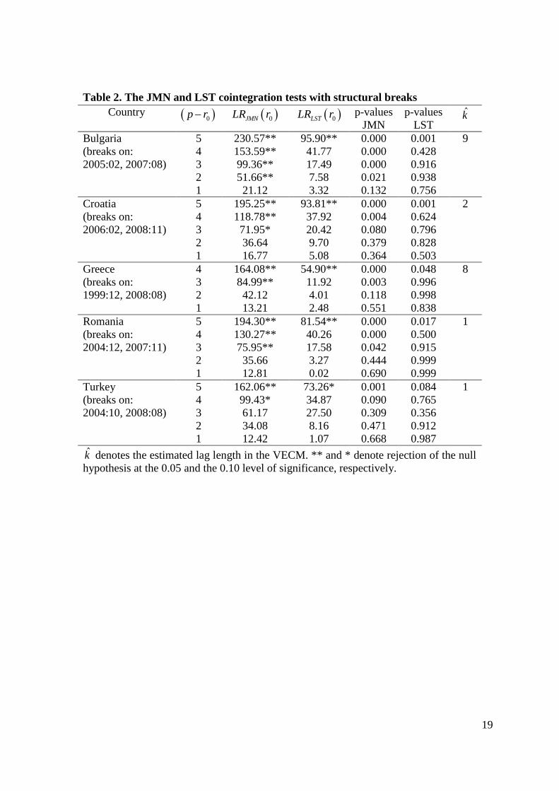
Table 2 reports the JMNLR and LSTLR test statistics and the respective p-values, for each

of the five sample countries. As shown in the table, the JMN test indicates four cointegrating

vectors for Bulgaria, three cointegrating vectors for Croatia and Romania, and two

cointegrating vectors for Greece and Turkey, either at the 5 or at 10 percent level of

significance. On the other hand, the LST test indicates a single cointegrating vector in each

2 The authors are grateful to Carsten Trenkler for kindly providing them with the Gauss codes for these

estimations.

12

case.3 As noted in Section 2.2, the LST test has better size and power properties than the JMN

test in finite samples. Thus, our subsequent analysis will be based on the results of the LST

test.

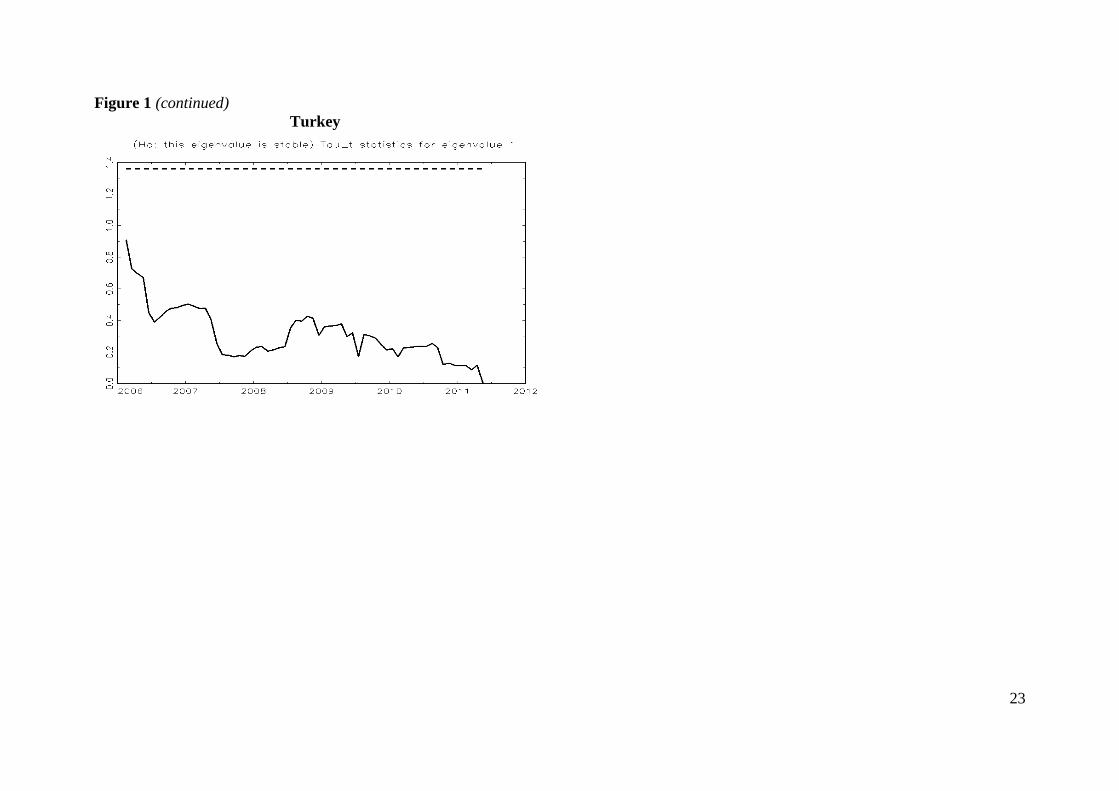
Note here, that the JMN and LST tests for cointegration in the presence of structural

breaks, assume that the ‘‘long-run’’ cointegration parameters remain constant over the sample

period. Otherwise, the test results and inference would be invalid. To test for parameter

constancy, we used the methodology developed by Hansen and Johansen (1999), who suggest

a graphical procedure based on recursively-estimated eigenvalues. Figure 1 shows the time

path of each eigenvalue (i.e. the sum -statistic) for the null hypothesis that it is stable. The

dotted line in each plot corresponds to 1.36, which is the 5 percent critical value for the

Hansen and Johansen parameter constancy test. The null hypothesis of long run parameter

constancy cannot be rejected in all cases, as the time paths of the eigenvalues are always

below the dotted line.4

3.4 VECMs and Orthogonal Impulse Responses

Based on the cointegration results of the previous section, we have established a valid

relationship, which can be interpreted as the long-run relationship between the industrial

production, the consumer price index, the money supply, the money market rate and the real

effective exchange rate. Following the above, we estimate the corresponding VECMs, based

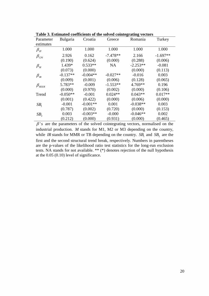
on equations (7a) and (7b). Table 3 presents the estimated coefficients of the solved

cointegrating vectors (i.e. reduced form equations) normalised on the industrial production,

along with the results from the long-run exclusion test. As shown in table 3 most of the

estimated coefficients have the expected signs. The long-run exclusion test investigates

whether any of the variables under consideration can be excluded from the cointegrating

space. Using the likelihood ratio test statistic, our results imply that the consumer price index

can be excluded from the cointegrating equation for Bulgaria, while both the consumer price

index and the real effective exchange rate can be excluded from the cointegrating equation for

Croatia. For Greece no variable can be excluded from the cointegration space. The consumer

price index and the money market rate can be excluded from the cointegrating equation for

Romania, while for Turkey, the money supply, the money market rate and the real effective

3 We have also performed the cointegration tests using diferrent combinations of structural breaks. The estimated

results did not change and are available upon request. 4 We have included centred seasonal dummies in the Hansen-Johansen tests, the VECM estimations and the

impulse responses.

13

exchange rate can be excluded from the cointegration space. When it comes to the implied

structural breaks, the long-run exclusion test shows that none of the breaks can be excluded

from the cointegrating space for Croatia and Romania. On the contrary, both structural

changes are found statistically insignificant for Bulgaria, Greece and Turkey in the long run.

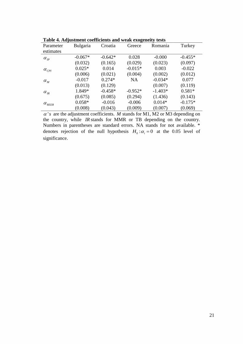
Also, we performed weak exogeneity tests, in order to investigate whether a variable

can be considered as weakly exogenous to the long-run parameters. A variable is said to be

weakly exogenous if the corresponding adjustment coefficient cannot be statistically different

from zero. The results for this test are reported in table 4 and provide us information about the

variables that drive the system to long-run equilibrium. Starting from the case of Bulgaria,

money supply is found to be weakly exogenous and, thus, drives the system to its long-run

equilibrium. For Croatia, consumer price index and real effective exchange rate are found to

be weakly exogenous, while for Greece, the driving forces of the system are the industrial

production and the real effective exchange rate. For Romania, industrial production and

consumer price index are found to be weakly exogenous, while for Turkey weak exogeneity

has been established for the consumer price index and the money supply.

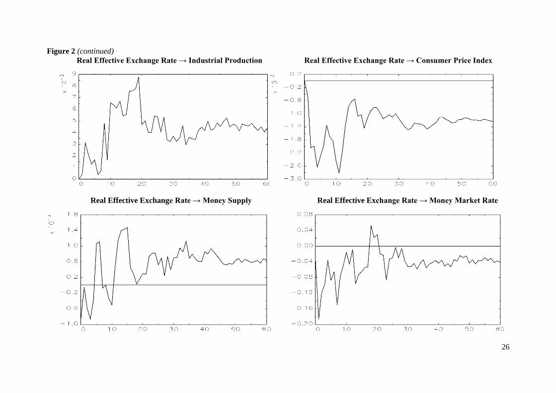
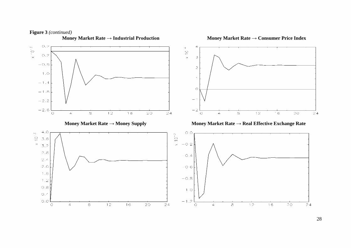
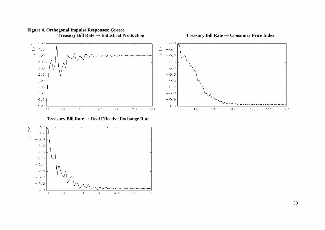
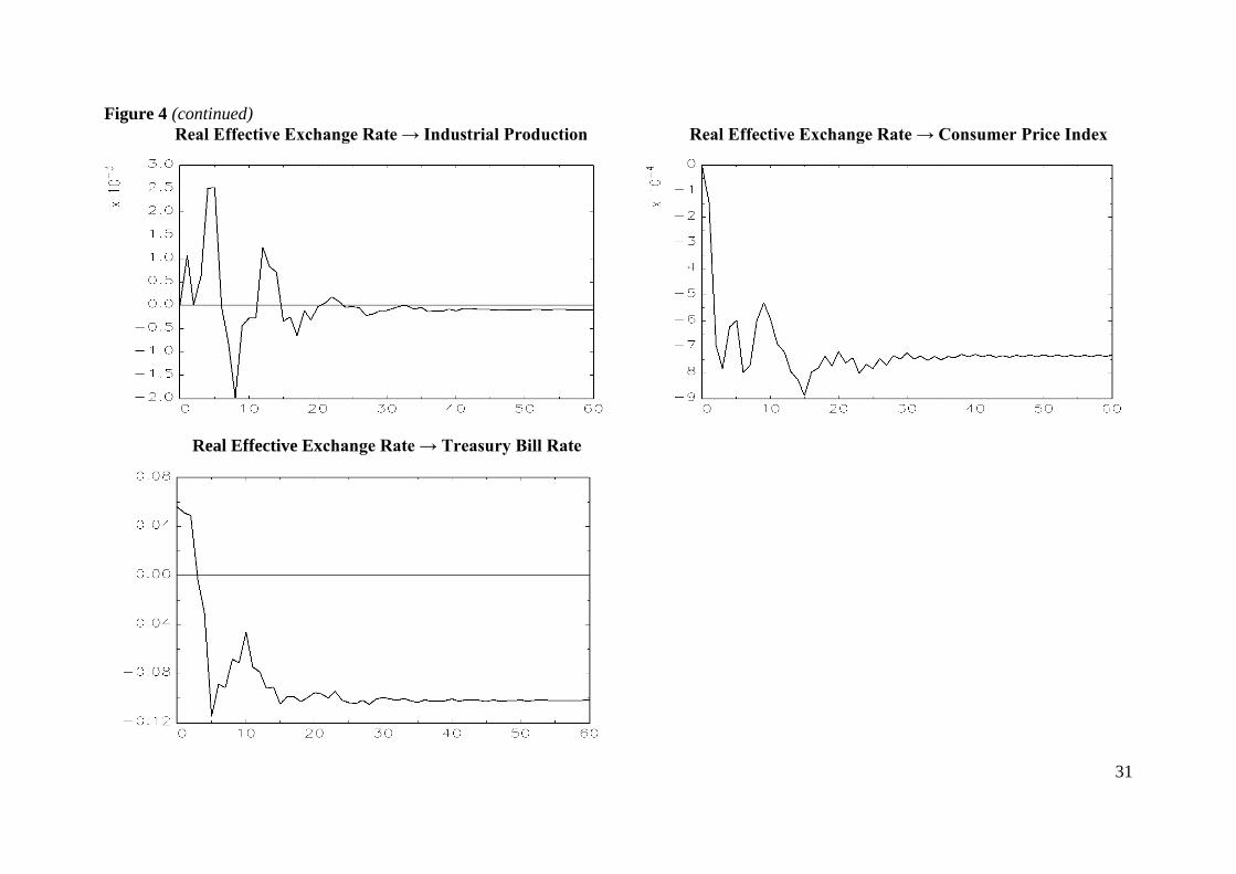
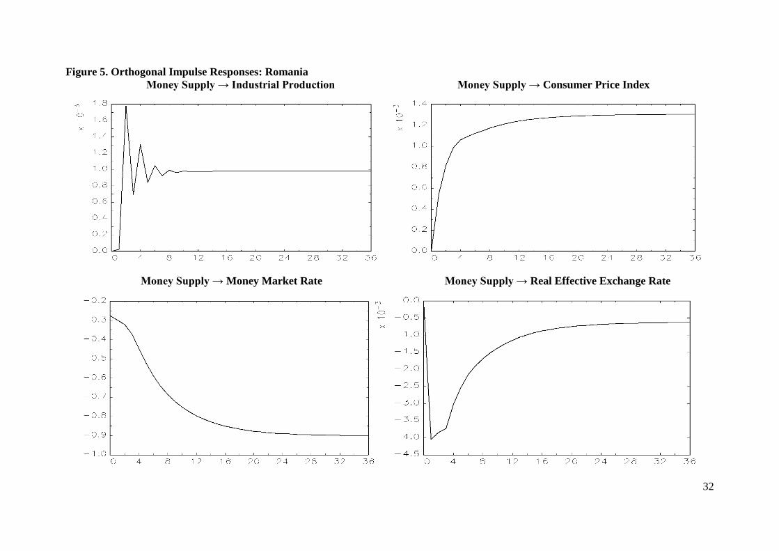
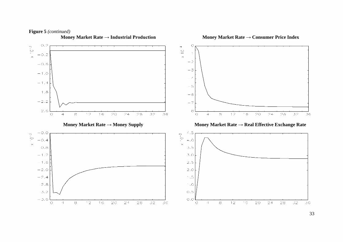
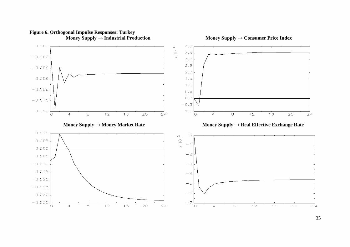
Finally, and in order to complete our analysis for the monetary transmission mechanism

in each country, we estimated orthogonal impulse response functions, based on an innovation

of one standard deviation in size, for each of the monetary variables (money supply and

money market rate or Treasury bill rate), as well as the real effective exchange rate. The

impulse responses are presented in figures 2 to 6. As shown, for the most of them the range of

values is of small magnitude. In general, they converge in all cases, implying stability of our

model, and seem reasonable. Only in the case of Turkey, the response of money market rate

to a shock in money supply and the response of industrial production to a shock in real

effective exchange rate do not converge to a stable level. A possible explanation for this

peculiar result could be attributed to the strong inflationary tendencies in the Turkish

economy.

4. Concluding Remarks

In the present we attempted to investigate the transmission mechanism for five South-Eastern

Europe countries, namely Bulgaria, Croatia, Greece, Romania and Turkey. We focused on the

monetary transmission through interest rate channel and real effective exchange rate channel.

Data limitations and the extreme heterogeneity of the above countries did not allow us to

construct a full structural model based on economic theory. Thus, we used a small reduced-

14

form model for each country, consisted of five endogenous variables, in order to establish a

valid long-run relationship and to analyse the impulse response functions. We also included

structural shifts in our analysis, since the implemented economic policies in the sample

countries are likely to have caused structural shifts in the level and trend of their variables

The unit root test results in the presence of structural breaks confirm the existence of

one or two breaks for each variable. The cointegration test results in the presence of structural

breaks show evidence of a single cointegrating vector with parameter constancy, among the

industrial production, the consumer price index, the money supply, the money market rate and

the real effective exchange rate, for each of the five countries under consideration. These

results identify a long-run relationship among the above variables, while the estimated

impulse response functions regarding the monetary variables and the real effective exchange

rate converge and seem reasonable in all cases. The present analysis regarding the monetary

transmission mechanism could be extended with the use of a global modelling framework,

based on the Global VAR (GVAR) model, which avoids all limitations that arise by the use of

single VAR and VECMs models and provides a consistent and flexible framework.

15

References

Bitâns, M. (2004), ‘Pass-Through of Exchange Rates to Domestic Prices in East European

Countries and the Role of Economic Environment’, Bank of Latvia Working Paper, No.

4.

Coricelli, F., Égert, B. and MacDonald, R. (2006), ‘Monetary Transmission Mechanism in

Central and Eastern Europe: Gliding on a Wind of Change’, Bank of Finland, Institute

for Economies in Transition, Discussion Paper 8.

Coricelli, F. Jazbec, B. and Masten, I. (2003), ‘Exchange Rate Pass-Through in Acceding

Countries: The Role of Exchange Rate Regimes’, Journal of Banking and Finance, 30

(5), 1375-1391.

Crespo-Cuaresma, J., Égert, B. and Reininger, T. (2004), ‘Interest Rate Pass-Through in New

EU Member States: The Case of the Czech Republic, Hungary and Poland’, William

Davidson Institute Working Paper, No. 671.

De Bondt, G. (2002), ‘Retail Bank Interest Rate Pass-Through: New Evidence at the Euro

Area Level’, European Central Bank Working Paper, No. 136.

Dabušinskas, A. (2003), ‘Exchange Rate Pass-Through to Estonian Prices’, Bank of Estonia

Working Paper, No. 10.

Darvas, Z. (2001), ‘Exchange Rate Pass-Through and Real Exchange Rate in EU Candidate

Countries’, Deutsche Bundesbank Discussion Paper, No. 10.

Égert, B., Crespo-Cuaresma, J. and Reininger, T. (2006), ‘Interest Rate Pass-Through in

Central and Eastern Europe: Reborn from Ashes to Pass Away?’, Focus on European

Economic Integration, No. 1.

Gueorguiev, N. (2003), ‘Exchange Rate Pass-Through in Romania’, IMF Working Paper, No.

130.

Hansen, H. and Johansen, S. (1999). ‘Some Tests for Parameter Constancy in Cointegrated

VAR-models’, Econometrics Journal, 2(2), 306-333.

Horváth, C., Krekó, J. and Naszódi, A. (2004), ‘Interest Rate Pass-Through: The Case of

Hungary’, National Bank of Hungary Working Paper, No. 8.

Johansen, S. (1988). ‘Statistical Analysis of Cointegration Vectors’, Journal of Economic

Dynamics and Control, 12(4), 231-254.

Johansen, S., Mosconi, R. and Nielsen, B. (2000). ‘Cointegration Analysis in the Presence of

Structural Breaks in the Deterministic Trend’, Econometrics Journal, 3(2), 216-249.

16

Kara, H., Küçük Tuğer, H., Özlale, Ü., Tuğer, B., Yavuz, D. and Yücel, E.M. (2005),

‘Exchange Rate Pass-Through in Turkey: Has It Changed and to What Extent?’, Central

Bank of the Republic of Turkey Working Paper, No. 4.

Korhonen, I. and Wachtel, P. (2005), ‘A Note on Exchange Rate Pass-Through in CIS

Countries’, Bank of Finland Discussion Paper, No. 2.

Lee, J. and Strazicich, M.C. (2003). ‘Minimum Lagrange Multiplier Unit Root Test with Two

Structural Breaks’, Review of Economics and Statistics, 85(4), 1082-1089.

Lütkepohl, H. and Saikkonen, P. (2000). ‘Testing for the Cointegrating Rank of a VAR

Process with a Time Trend’, Journal of Econometrics, 95(1), 177-198.

Lütkepohl, H., Saikkonen, P. and Trenkler, C. (2003). ‘Comparison of Tests for the

Cointegrating Rank of a VAR Process with a Structural Shift’, Journal of Econometrics,

113(2), 201-229.

Mihaljek, D. and Klau, M. (2001), ‘A Note on the Pass-Through from Exchange Rate and

Foreign Price Changes to Inflation in Selected Emerging Market Economies’, Bank of

International Settlements Paper, No. 8.

Opiela, T. P. (1999), ‘The Responsiveness of Loan Rates to Monetary Policy in Poland: The

Effects of Bank Structure’, National Bank of Poland Materials and Studies, No. 12.

Perron, P. (1989). ‘The Great Crash, the Oil Price Shock, and the Unit Root Hypothesis’,

Econometrica, 57(6), 1361-1401.

Perron, P. (1993). ‘Erratum: The Great Crash, the Oil Price Shock, and the Unit Root

Hypothesis’, Econometrica, 61(1), 248-249.

Saikkonen, P. and Lütkepohl, H. (2000). ‘Testing for the Cointegrating Rank of a VAR

Process with Structural Shifts’, Journal of Business and Economic Statistics, 18(4),

451-464.

Sander, H. and Kleimeier, S. (2004a), ‘Convergence in Euro-Zone Retail Banking? What

Interest Rate Pass-Through Tells Us about Monetary Policy Transmission, Competition

and Integration’, Journal of International Money and Finance, 23(3), 461.492.

Sander, H. and Kleimeier, S. (2004b), ‘Interest Rate Pass-Through in an Enlarged Europe:

The Role of Banking Market Structure for Monetary Policy Transmission in Transition

Economies’, University of Maastricht, METEOR Research Memoranda, No. 45.

Trenkler, C. (2008). ‘Determining P-values for Systems Cointegration Tests with a Prior

Adjustment for Deterministic Terms’, Computational Statistics, 23(1), 19-39.

17

Trenkler, C., Saikkonen, P. and Lütkepohl, H. (2008) ‘Testing for the Cointegrating Rank of a

VAR Process with Level Shift and Trend Break’, Journal of Time Series Analysis,

29(2), 331-358.

18

Table 1: Two-break minimum LM unit root test results

Country Variable Model

k̂ ˆ

BT

1 2ˆ ˆ, LM statistic

Bulgaria IP

CPI

M3

MMR

REER

C

C

C

C

C

12

12

12

10

2

2003:12, 2008:08

2002:04, 2007:10

2005:02, 2007:08

2001:12, 2009:02

2007:10, 2010:01

0.4, 0.8

0.2, 0.6

0.4, 0.6

0.2, 0.8

0.6, 0.8

-5.4237

-4.4316

-4.4335

-4.0249

-5.0334

Croatia IP

CPI

M1

MMR

REER

C

C

C

C

C

11

12

12

1

1

2006:02, 2008:10

2006:03n, 2008:01

2005:03n, 2008:11

2008:02n, 2008:11

2007:11, 2010:01

0.4, 0.8

0.4, 0.6

0.4, 0.8

0.6, 0.8

0.6, 0.8

-5.6393

-4.5633

-3.9050

-5.6928

-5.5588

Greece IP

CPI

TB

REER

C

C

C

C

11

10

6

12

1999:12, 2008:08

1999:02, 2001:10

2004:02, 2008:09

1999:02, 2002:11

0.4, 0.8

0.2, 0.4

0.6, 0.8

0.2, 0.4

-5.5307

-5.0288

-3.9003

-5.2925

Romania IP

CPI

M2

MMR

REER

C

C

C

C

C

12

10

12

6

1

2008:08, 2010:03

2003:07, 2005:01

2004:12, 2007:11

2006:09, 2009:03

2004:11, 2007:10

0.6, 0.8

0.2, 0.4

0.4, 0.6

0.4, 0.8

0.4, 0.6

-5.4496

-4.3414

-4.8818

-4.7614

-4.4244

Turkey IP

CPI

M3

MMR

REER

C

C

C

C

C

12

12

6

3

1

2008:09, 2009:10

2004:10, 2007:11

2005:10, 2007:07

2004:10, 2006:10

2008:04, 2009:12

0.6, 0.8

0.2, 0.6

0.4, 0.6

0.2, 0.4

0.6, 0.8

-5.5628

-5.2050

-5.1521

-5.2923

-4.7017

Break Points Critical values for Model C

1 2, 1% 5%

λ=(0.2, 0.4)

λ=(0.2, 0.6)

λ=(0.2, 0.8)

λ=(0.4, 0.6)

λ=(0.4, 0.8)

λ=(0.6, 0.8)

-6.16

-6.41

-6.33

-6.45

-6.42

-6.32

-5.59

-5.74

-5.71

-5.67

-5.65

-5.73

k̂ is the estimated number of to correct for serial correlation. ˆBT denotes the estimated

break points. 1̂ and 2̂ are the estimated relative break points. IP stands for industrial

production, CPI for consumer price index, M1, M2 and M3 for money supply, MMR for

money market rate, TB for Treasury bill rate, and REER for real effective exchange rate. n

indicates no significant break at the 10 percent level of significance. The critical values are

from table 2 of Lee and Strazicich (2003).

19

Table 2. The JMN and LST cointegration tests with structural breaks

Country 0p r 0JMNLR r 0LSTLR r

p-values

JMN

p-values

LST k̂

Bulgaria

(breaks on:

2005:02, 2007:08)

5

4

3

2

1

230.57**

153.59**

99.36**

51.66**

21.12

95.90**

41.77

17.49

7.58

3.32

0.000

0.000

0.000

0.021

0.132

0.001

0.428

0.916

0.938

0.756

9

Croatia

(breaks on:

2006:02, 2008:11)

5

4

3

2

1

195.25**

118.78**

71.95*

36.64

16.77

93.81**

37.92

20.42

9.70

5.08

0.000

0.004

0.080

0.379

0.364

0.001

0.624

0.796

0.828

0.503

2

Greece

(breaks on:

1999:12, 2008:08)

4

3

2

1

164.08**

84.99**

42.12

13.21

54.90**

11.92

4.01

2.48

0.000

0.003

0.118

0.551

0.048

0.996

0.998

0.838

8

Romania

(breaks on:

2004:12, 2007:11)

5

4

3

2

1

194.30**

130.27**

75.95**

35.66

12.81

81.54**

40.26

17.58

3.27

0.02

0.000

0.000

0.042

0.444

0.690

0.017

0.500

0.915

0.999

0.999

1

Turkey

(breaks on:

2004:10, 2008:08)

5

4

3

2

1

162.06**

99.43*

61.17

34.08

12.42

73.26*

34.87

27.50

8.16

1.07

0.001

0.090

0.309

0.471

0.668

0.084

0.765

0.356

0.912

0.987

1

k̂ denotes the estimated lag length in the VECM. ** and * denote rejection of the null

hypothesis at the 0.05 and the 0.10 level of significance, respectively.

20

Table 3. Estimated coefficients of the solved cointegrating vectors

Parameter

estimates

Bulgaria Croatia Greece Romania Turkey

IP 1.000 1.000 1.000 1.000 1.000

CPI 2.926

(0.190)

0.162

(0.624)

-7.478**

(0.000)

2.166

(0.288)

-1.697**

(0.006)

M 1.439*

(0.073)

0.533**

(0.000)

NA -2.253**

(0.000)

-0.081

(0.113)

IR -0.137**

(0.009)

-0.004**

(0.001)

-0.027**

(0.006)

-0.016

(0.128)

0.003

(0.065)

REER 5.783**

(0.000)

-0.009

(0.970)

-1.553**

(0.002)

4.769**

(0.000)

0.196

(0.106)

Trend -0.050**

(0.001)

-0.001

(0.422)

0.024**

(0.000)

0.043**

(0.006)

0.017**

(0.000)

1SB -0.001

(0.787)

-0.001**

(0.002)

0.001

(0.720)

-0.038**

(0.000)

0.003

(0.153)

2SB 0.003

(0.212)

-0.003**

(0.000)

-0.000

(0.931)

-0.046**

(0.000)

0.002

(0.465)

's are the parameters of the solved cointegrating vectors, normalised on the

industrial production. M stands for M1, M2 or M3 depending on the country,

while IR stands for MMR or TB depending on the country. 1SB and 2SB are the

first and the second structural trend break, respectively. Numbers in parentheses

are the p-values of the likelihood ratio test statistics for the long-run exclusion

tests. NA stands for not available. ** (*) denotes rejection of the null hypothesis

at the 0.05 (0.10) level of significance.

21

Table 4. Adjustment coefficients and weak exogeneity tests

Parameter

estimates

Bulgaria Croatia Greece Romania Turkey

IP -0.067*

(0.032)

-0.642*

(0.165)

0.028

(0.029)

-0.000

(0.023)

-0.455*

(0.097)

CPI 0.025*

(0.006)

0.014

(0.021)

-0.015*

(0.004)

0.003

(0.002)

-0.022

(0.012)

M -0.017

(0.013)

0.274*

(0.129)

NA -0.034*

(0.007)

0.077

(0.119)

IR 1.849*

(0.675)

-0.458*

(0.085)

-0.952*

(0.294)

-1.403*

(1.436)

0.581*

(0.143)

REER 0.058*

(0.008)

-0.016

(0.043)

-0.006

(0.009)

0.014*

(0.007)

-0.175*

(0.069)

's are the adjustment coefficients. M stands for M1, M2 or M3 depending on

the country, while IR stands for MMR or TB depending on the country.

Numbers in parentheses are standard errors. NA stands for not available. *

denotes rejection of the null hypothesis 0 : 0iH at the 0.05 level of

significance.

22

Figure 1. Parameter constancy tests ( sum -statistics)

Bulgaria Croatia

Greece Romania

23

Figure 1 (continued)

Turkey

24

Figure 2. Orthogonal Impulse Responses: Bulgaria

Money Supply → Industrial Production Money Supply → Consumer Price Index

Money Supply → Money Market Rate Money Supply → Real Effective Exchange Rate

25


Money Market Rate → Industrial Production Money Market Rate → Consumer Price Index

Money Market Rate → Money Supply Money Market Rate → Real Effective Exchange Rate

26


Real Effective Exchange Rate → Industrial Production Real Effective Exchange Rate → Consumer Price Index

Real Effective Exchange Rate → Money Supply Real Effective Exchange Rate → Money Market Rate

27

Figure 3. Orthogonal Impulse Responses: Croatia



28




29




30

Figure 4. Orthogonal Impulse Responses: Greece

Treasury Bill Rate → Industrial Production Treasury Bill Rate → Consumer Price Index

Treasury Bill Rate → Real Effective Exchange Rate

31



Real Effective Exchange Rate → Treasury Bill Rate

32

Figure 5. Orthogonal Impulse Responses: Romania



33




34




35

Figure 6. Orthogonal Impulse Responses: Turkey



36




37




Transmission Effects in the Presence of Structural Breaks...

Documents

Transcript of Transmission Effects in the Presence of Structural Breaks...