Working Paper 2006:11Department of Economics

Structural Breaks in Iron-OrePrices: The Impact of the 1973Oil Crisis

Nikolay Angelov

Department of Economics Working paper 2006:11Uppsala University January 2006P.O. Box 513 ISSN 1653-6975SE-751 20 UppsalaSwedenFax: +46 18 471 14 78

STRUCTURAL BREAKS IN IRON-ORE PRICES: THE IMPACT OF THE 1973 OIL CRISIS

NIKOLAY ANGELOV

Papers in the Working Paper Series are publishedon internet in PDF formats.Download from http://www.nek.uu.seor from S-WoPEC http://swopec.hhs.se/uunewp/

Structural Breaks in Iron-Ore Prices:

The Impact of the 1973 Oil Crisis∗

Nikolay Angelov†

January 20, 2006

Abstract

This paper investigates the time-series properties of the price of iron ore. The

focus is on testing a unit-root null hypothesis against a trend-stationary alternative,

with a structural break allowed under both hypotheses. We consider unit-root

tests with or without structural breaks, applied on historical prices of five different

qualities of Swedish and Brazilian iron ore. New and more accurate critical values

for the exogenous-break tests are calculated, and several of the asymptotic tests are

accompanied by their bootstrap counterparts due to the limited sample sizes.

Using unit-root tests allowing for an exogenous structural break in 1973, the null

hypothesis of a unit root is rejected for three of the five series. The sign and nature

of the estimated breaks correspond to the state of the iron and steel industry during

the first half of the 1970s. The bootstrap tests give results close to those from the

asymptotic ones.

Key words: iron-ore prices; structural break; unit-root test; bootstrap

JEL classification: C15; C22; Q30

∗The author is indebted to Rolf Larsson, Lars Hultkrantz, Abdulnasser Hatemi-J, and Steinar Strømfor useful advice. Suggestions from participants at a seminar at the Department of Statistics, UppsalaUniversity, and from Johan Lyhagen in particular, are gratefully acknowledged. Comments from par-ticipants at the conference on Unit Root and Cointegration Testing in Faro, Portugal, 29 September–1October 2005 are appreciated.

†Address: Department of Economics, Uppsala University, Box 513, SE-751 20, Uppsala, Sweden.E-mail: nikolay.angelov@nek.uu.se

1 Introduction

This paper deals with the time-series properties of Swedish and Brazilian iron ore. We

focus on unit-root testing, and more specifically, unit-root tests that allow for structural

breaks. Before stating the purpose and delimitations of the paper, a motivation for

research in the field will be given, followed by a short survey of the literature on structural-

break unit-root tests and an overview of earlier studies of the empirical properties of

commodity prices.

Whether prices of mineral commodities are mean-reverting or follow a random walk

is important for several reasons. Firstly, as noted in Schwartz (1997), the stochastic

behaviour of commodity prices has important implications for the valuation of projects

related to them, for instance mines or oil plants. The optimal investment rule, denoted by

p∗, is the commodity price above which it is optimal to undertake the project. It depends

on the underlying price process of the commodity. Schwartz analyzes an investment

project in a copper mine and evaluates it using three different mean-reverting models

for the underlying commodity. The results are then compared with a case where the

underlying process follows a geometric random walk. The study suggests that the real

options approach induces investment too late (i.e., when prices are too high) when mean

reversion in prices is neglected.1

Also Metcalf and Hassett (1995) investigate this matter, but come to the conclusion

that although mean reversion has an influence on investment, there are two opposing

effects which, on average, offset each other. Mean reversion has the effect of reducing the

volatility of project returns, thereby reducing p∗; this has a positive effect on investment.

But there is also a negative effect: the maximum price that will be achieved over a

given time period will decrease when mean reversion is introduced, thus decreasing the

likelihood of reaching the trigger value.

In a recent paper, Sarkar (2003) acknowledges the two latter effects, but adds a third

one, namely what he calls the risk-discounting effect. The intuition is that when mean

reversion is introduced, the volatility of project returns falls, hence a lower risk-adjusted

discount rate should be used for project evaluation. The lower discount rate works in

two opposite directions: It results in a higher project value, and (since the option to

invest can be seen as a put option and Sarkar assumes stochastic costs) it increases the

option value. Sarkar’s conclusion is that using a geometric random walk to approximate

a mean-reverting process might have a significant impact on investment. For short-lived

projects, mean reversion is more likely to have a negative impact on investment, while

the effect on long-lived projects is expected to be positive. In either case, Sarkar asserts

that approximating a mean-reverting process with a random walk is not justifiable.

1See Schwartz (1997, Table XX, p. 967) for the complete set of results.

1

Secondly, another characteristic of a random walk is of importance, namely the fact

that shocks have a permanent effect on the level of the series, rather than dying out with

time. The persistence of shocks is important for the design of short- and long-term policies

in countries that are largely dependent on export of a certain commodity. For instance,

the optimal management of stabilization funds depends on the nature and persistence of

shocks in commodity prices.

The rest of this section is organized as follows: After a short history of structural-

break unit-root testing for macroeconomic time series, the literature with applications

to commodities is surveyed. This is followed by a motivation for and an outline of the

present paper.

Ever since the influential article by Nelson and Plosser (1982), the question of whether

shocks have a transitory or a permanent effect on macroeconomic time series has been

thoroughly studied. Using the augmented Dickey-Fuller test and a data set consisting of

14 macroeconomic time series, Nelson and Plosser accept the null hypothesis for almost

all of the investigated series.

Perron (1989) challenges these results by postulating that only the Great Crash in 1929

and the oil-price shock in 1973 have had permanent effects on the series included in the

Nelson and Plosser data set. By introducing a new test procedure, allowing for a one-

time change in the level, in the slope, or both in the level and in the slope of the trend

function, Perron rejects the unit-root hypothesis for 11 out of the 14 series. The oil-price

shock and the Great Crash are modelled as exogenous shocks, in the sense that they are

not realizations of the data generating processes of the various series. Instead, they are

assumed to occur at an a priori known date.

The latter approach has been criticized and new methods have been proposed. One of

the objections concerns the assumption of an exogenous break with a known date. Chris-

tiano (1992) asserts that in practice, one never selects a break date without prior informa-

tion about the data. Neglecting this pre-test examination gives p-values which overstate

the likelihood of the trend-break alternative hypothesis. Consequently, in Christiano’s

study pre-testing is taken into account, and bootstrap testing of the null hypothesis of a

unit root in GNP results in high observed p-values.

The approach in Zivot and Andrews (1992) is similar to that of Christiano in its search

for a break, but instead of solely relying on bootstrap methods, the asymptotic distri-

butions of the test statistics are derived. Besides that, the finite sample distributions of

the test statistics are estimated using Monte Carlo methods. Using both the asymptotic

critical values and the finite-sample distributions, the study finds less conclusive evidence

against the unit-root hypothesis than Perron on the Nelson and Plosser data set.

Another issue that has been discussed is the number of structural breaks in the testing

procedures. By applying a model with two endogenous breaks on the Nelson and Plosser

2

data set, a study by Lumsdaine and Papell (1997) shows results that lie somewhere in

between those of Zivot and Andrews, and Perron. The authors emphasize the importance

of model selection in determining both the number of breaks and the type of break, rather

than a specific preference for two endogenous breaks.

Accordingly, some studies have focused on explicit testing schemes for the number of

structural breaks. One of the latest contributions is the one by Bai and Perron (2003),

where a general procedure for estimation of the break dates in multiple structural change

models is presented. In addition, a procedure that allows one to test the null hypothesis

of l changes versus the alternative hypothesis of l + 1 changes is proposed. The study is

concerned with estimation, and not specifically with unit-root testing.

Mineral prices have received much less attention than macroeconomic series in the

empirical literature on unit-root testing, and even less in the case when structural change

is allowed. One of the earlier contributions to time-series modelling of non-renewable

commodity prices is the one by Slade (1982). She introduces a theoretical model for

long-run price movements of mineral commodities, suggesting a U-shaped time path for

the price process. An economic intuition is that initially, technological change implies

falling prices, while in the long run, scarcity dominates the price process and prices rise.

The empirical part of the article consists of fitting the simplest U-shaped time path, the

quadratic trend, to eleven non-renewable commodities’ deflated prices, among those pig

iron. For most of the series, Slade finds the simple equation

pt = α + β1t + β2t2 + vt

suitable. For all commodities, however, the residuals are found to be severely first-order

serially correlated. Instead of adding AR-terms in the regression, the OLS-estimates are

adjusted for autocorrelation.

Jumping some ten years ahead in time, Agbeyegbe (1993) uses partly the same data

set as Slade, but with another focus. He clearly addresses the issue of unit-root testing,

applying several unit-root tests to the deflated price series. In those tests, he allows

for a quadratic time trend in the data. Agbeyegbe concludes that three out of the four

analyzed price series, including pig iron, are adequately represented as processes with a

unit root and a quadratic time trend. Several issues not considered in the article but worth

investigating are raised by the author, including the possibility of a structural change in

the series.

The subsequent study by Ahrens and Sharma (1997) takes the analysis still further,

including, among other tests, a unit-root test allowing for a trend break. They choose

one of the six types of models introduced in Perron (1989), a model allowing for an

instantaneous break both in the level and in the slope of the linear trend function at

different globally important events. Those are the Great Crash in 1929, the outbreak of

3

World War II in 1939, and the end of the war in 1945. For each analyzed non-renewable

commodity, the structural breaks unit-root test is applied while assuming a single break

at any of the dates. Four out of eight analyzed series, among those pig iron, appear to be

trend stationary when allowing for a possible structural break.

Two things should be borne in mind when interpreting Ahrens’ and Sharma’s results:

First, the model by Perron assumes only one exogenous break. If that exogenous break

date is changed, and the test still results in a rejection of the null hypothesis of a unit root,

some ambiguities may arise as to when the break occurs. Perhaps a model with multiple

exogenous breaks would be more suitable to use. Second, the authors do not take into

account Perron and Vogelsang (1993), where it is stated that the limiting distribution

and critical values of the test statistic from the earlier paper by Perron are incorrect. In

order to be able to use the critical values, a dummy variable must be added to the test

regression used by Ahrens and Sharma.

Still one relevant study is that by Leon and Soto (1997). While the previously described

article only uses the structural breaks test as one among other unit-root tests, Leon and

Soto explicitly focus on structural breaks testing procedures. Also, the data consist of

both non-renewable and renewable commodities. The authors rely on the procedure

introduced by Zivot and Andrews (1992), which endogenizes the choice of structural

break. The model builds on Perron (1989), but instead of assuming an exogenous break,

a data-dependent search routine is introduced, with corresponding critical values for the

unit-root test statistic. The only non-renewable commodities analyzed are aluminium,

copper, and silver. Allowing for a break in the level, or in the trend function, of the

aluminium series rejects the unit-root null hypothesis at the ten percent level. For the

copper series, the null is rejected at the ten percent level only when allowing for a break

in the level of the series. The silver price series seems to be better parameterized as

difference stationary.

One of the latest contributions is due to Howie (2002). The study applies several unit-

root tests, with different trend function specifications, to 12 different mineral commodity

price series. This study is the only one of those mentioned so far that includes an iron

ore series in the analysis. The price series pertains to US-produced iron ore, and is found

to be difference stationary; in other words, none of the four different tests reject the null

hypothesis of a unit root. For the pig iron price series included, two of the tests (the

augmented Dickey-Fuller test with a linear trend and a unit-root test with a quadratic

trend) reject the unit-root null hypothesis.

The present study contributes to the previous literature in several ways. Firstly, none of

the previously mentioned studies applies structural-break unit-root tests to iron-ore prices.

As already mentioned, Howie (2002) analyses iron-ore prices, but excludes the possibility

of structural breaks. We argue that any analysis concerning the time-series properties of

4

iron-ore prices should take into account the state of the iron and steel industry during the

first half of the 1970s, as described in OECD (1975) and OECD (1976) (see section 4.2).

Relative to other prices in the economy, the unusually high demand for steel during that

period ought to have resulted in a positive price shock for iron ore.

Secondly, instead of using only a few structural-break unit-root tests among those

available, we apply various tests with a single exogenous break, with a single endogenous

break and several ways of selecting the break date, and finally tests with two endogenous

breaks. All these are modifications of the well-known augmented Dickey-Fuller (ADF)

test, which is also applied to the series.

Finally, on the more technical side, new and more accurate critical values are calculated

for the exogenous-break tests. Furthermore, we do not merely rely on asymptotic tests.

Several of the exogenous break tests, and also the ADF-test, are bootstrapped, mainly

due to the limited sample sizes of the series.

Thus, the purpose of this study is to investigate whether the examined time series

exhibit a unit root, if we allow for a structural break at an a priori known or unknown

date, or at two unknown dates.

Several delimitations are made:

Perhaps the most important is the choice of data. The global market for iron ore

consists of two markets—an Asian market and a European one—and this paper focuses

on the latter. That being so, a motivation for the choice of specific price series from the

European market is given in section 3.

Furthermore, all tests exhibit linear trend functions. Since the natural logarithm of the

series is used in the analysis (see section 3), this implies exponential trends in the levels of

the series. A quadratic time trend might be more appropriate (see the passage on earlier

studies above), but no structural-break unit-root tests allowing for a quadratic trend are

available to the author.

Finally, the focus is on tests allowing for a structural break, and thus only the ADF-

test—among an ocean of no-break unit-root tests—is considered in the analysis.

The remaining part of the paper is organized as follows: The next section describes all

models used, and is followed by a description of the data. After a section on the empirical

results, the main findings are concluded. A description of the bootstrap tests used, the

routine for calculating critical values, some of the tables, and all figures, can be found in

various appendices.

2 Models for unit-root testing

In this section, the models used for unit-root testing are accounted for. We begin with the

well known augmented Dickey-Fuller test, followed by a description of a number of tests

with exogenous or endogenous structural breaks, and with one or two possible breaks.

5

2.1 Augmented Dickey-Fuller (ADF) test

There are many different unit-root tests available, many of those surveyed in Maddala and

Kim (1998). The ADF-test is chosen here largely because it is the building block of the

structural-break tests to be described later on; the main purpose of this paper is to apply

the structural-break models, and with that in mind, a comparison with the ADF-test is

relevant.

The general testing equation is

pt = α + ρpt−1 +k∑

j=1

γj∆pt−j + βt + ut, (1)

where ∆pt = pt − pt−1 and ut ∼ i.i.d.(0, σ2). The null hypothesis is that of a unit root,

ρ = 1, while the alternative is a trend stationary process with ρ < 1.

One way of testing for unit root under this specification is to use the test statistic

τρ =ρ− 1

σρ

.

Under H0, τρ does not converge to a t-distribution in large samples; critical values can

instead be found in many standard books in econometrics, for instance Hamilton (1994,

Table B.6, p. 763).

Popular as this τ -test may be, it is somewhat debatable. In fact, under H0, ρ = 1

implies β = 0;2 thus, we would actually want to test

H0 : {ρ = 1 and β = 0} against H1 : {ρ < 1 and β 6= 0}. (2)

If only the τ -statistic is used, there is an ambiguity as to how to interpret the coefficients

under the null and under the alternative. For instance, under the alternative hypothesis,

α is the level of the series and β is the coefficient of the linear trend. But under the null,

α is the coefficient corresponding to t, while β is the coefficient corresponding to t2 in a

quadratic trend specification.

Now, testing (2) is by no means a standard procedure, since the sign of ρ is incorporated

in the alternative.3 Abadir and Distaso (2003) propose a new class of statistics for testing

similar hypothesis. In our setting, the test statistic would be a sum with of independent

statistics: one for testing ρ = 1 against ρ < 1, and another for testing β = 0 against

β 6= 0.

But here, we instead rely on an F -statistic for testing

2See for instance Maddala and Kim (1998, p. 38–39)3The reason for specifying the direction is that, in analogy with the τ -test above, we would like to

rule out the explosive case.

6

H0 : {ρ = 1 and β = 0} against H1 : {ρ 6= 1 and β 6= 0}, (3)

i.e., a test not ruling out the explosive case.4 The test statistic Φ3 from Dickey and

Fuller (1981) is equivalent to a standard regression F -test for performing (3), so it is

well-suited to our needs. Besides critical values based on the asymptotic distribution of

Φ3, Table VI in that article provides simulated finite sample critical values, not deviating

much from the asymptotical quartiles. We use the former for sample sizes of 50.

When the test regression is estimated, a data-dependent procedure is used to find the

optimal k, the number of lag parameters included in the regression. The routine is a

general-to-specific one and it chooses k so that the coefficient on the last included lagged

difference is significant at the 10%-level, while it is insignificant for larger ks, up to a

maximum lag length of kmax. For further reference, we call this procedure k-sig.

Ng and Perron (1995) compare the properties of this general-to-specific routine with

other ways of selecting the lag length (i.e., information criteria). They conclude that the

sequential procedure may result in a certain loss of power due to overparametrization,

while the often too parsimonious model chosen with the different information criteria

results in more severe size distortions. Thus, the sequential procedure is recommended.

A discussion on different methods for choosing k can also be found in Maddala and Kim

(1998, pp. 77–78).

The F - and τ -tests based on simulated critical values are accompanied by corresponding

model-based bootstraps. For details on the latter, see appendices A.1, A.2, and A.5.

2.2 Unit-root testing when a structural break is allowed

Perron (1989) suggests a unit-root test, where both under the null and the alternative

hypotheses, an exogenous one-time change in the level, in the slope, or both in the level

and in the slope of the trend function is allowed for. The study shows how standard tests

for unit root against the alternative of trend stationarity fail to reject the null even if the

true data generating process is that of stationary fluctuations around a trend function

which contains a one-time break.

Perron extends the Dickey-Fuller testing strategy to ensure a consistent testing proce-

dure against shifting trend functions. The tests are applied to a number of macroeconomic

time series, and for most of the series, the null is rejected. The only shocks that are found

to have permanent effect are the 1929 crash and the 1973 oil-price shock.

Three models under the null hypothesis are considered, denoted by A,B, and C, with

4This approximation of the directional test with an ordinary F -test can be expected to be quiteaccurate for the data used in this paper. In the bootstrap tests described in appendix A.5, the fractionof δ-estimates that were larger than zero were estimated. For none of the five investigated series thefraction was larger than one percent, implying that a double-sided test—for practical purposes and forour data—is almost equivalent to a directional one.

7

corresponding models under the alternative. Given a series {pt}T0 , the hypotheses are as

follows:

Models under the null:

(A) pt = µ + dD(TB)t + pt−1 + et,

(B) pt = µ1 + pt−1 + (µ2 − µ1)DUt + et, and (4)

(C) pt = µ1 + pt−1 + dD(TB)t + (µ2 − µ1)DUt + et,

where

D(TB)t = 1 if t = TB + 1, 0 otherwise;

DUt = 1 if t > TB, 0 otherwise; and

A(L)et = B(L)ξt,

ξt ∼ i.i.d.(0, σ2), with A(L) and B(L) pth and qth polynomial, respectively, in the lag

operator L. Thus, the innovation series {et} is taken to be of the ARMA(p, q) type with

(p, q) possibly unknown.

Models under the alternative:

(A) pt = µ1 + βt + (µ2 − µ1)DUt + νt,

(B) pt = µ + β1t + (β2 − β1)DT ∗t + νt, and (5)

(C) pt = µ1 + β1t + (µ2 − µ1)DUt + (β2 − β1)DTt + νt,

where

DT ∗t = t− TB if t > TB, 0 otherwise,

DTt = t if t > TB, 0 otherwise, and

νt ∼ ARMA(p + 1, q).

Under both the null and the alternative, TB refers to the time of the structural break,

i.e., the period at which the change in the parameters of the trend function occurs.5

Model (A) is called the crash model. Under the unit-root null, the model allows for

a one-time shock at TB. The alternative hypothesis of trend-stationarity allows for a

one-time shift in the intercept of the trend function. Model (B) is referred to as the

5The relations between the null and the alternative hypotheses might not be obvious, but in fact the

8

changing growth model. Under the alternative hypothesis, a change in the slope of the

trend function without any sudden change in the level at the time of the break is allowed

for. Model (C) allows for both effects to take place simultaneously, i.e., a sudden change

in the level of the series, followed by a different growth path.

The methods above imply that the structural break occurs instantaneously, which does

not need to be the case. Perron suggests an extension, where it is supposed that the time

series reacts gradually to a shock function. Consider, for instance, the deterministic part

of the alternative of Model (A). From (5) we can write it as

ηAt = µ1 + βt + γDUt,

where γ = (µ2− µ1). Perron calls this a trend function, and we adhere to that denota-

tion. A plausible adjustment is to define the trend function as

ηAt ≡ µ1 + βt + γψ(L)DUt,

where ψ(L) is an invertible polynomial in L with ψ(0) = 1. The long-run change in

the level is given by γψ(L) while the immediate impact is simply γ. A similar framework

holds for models (B) and (C).

One way to incorporate such a gradual change in the trend function is to suppose

that the series responds to a shock in the trend function the same way as it reacts to

any innovation. This can be achieved by imposing ψ(L) = B(L)−1A(L). Nesting the

corresponding models under the null and the alternative hypotheses results in the following

regressions:6.

null is a special case of the alternative. For instance, in the case of Model (A) we can write the null as

pt = µ + dD(TB)t + pt−1 + et

= µ + dD(TB)t + (µ + dD(TB)t−1 + pt−2 + et−1) + et

= p0 + µt + d

t−1∑

j=0

D(TB)t−j +t−1∑

j=0

et−j

= p0 + µt + dDUt + vt

≡ µ1 + βt + (µ2 − µ1)DUt + νt,

where vt = (vt−1 + et) ∼ ARIMA(p, 1, q). Now, an ARIMA(p, 1, q) process can be seen as a special caseof an ARMA(p + 1, q) process with the first autoregressive coefficient equal to one. Thus, for Model (A),the null hypothesis is a special case of the alternative, and in a similar way the same holds for Models(B) and (C).

6For details on why DUt is missing from the RHS of the equation for Model (B), see Perron (1989, p.1381)

9

(A) pt = µA + βAt + θADUt

+dAD(TB)t + αApt−1 +k∑

i=1

cAi ∆pt−i + et,

(B) pt = µB + βBt (6)

+γBDT ∗t + αBpt−1 +

k∑i=1

cBi ∆pt−i + et, and

(C) pt = µC + βCt + θCDUt

+γCDTt + dCD(TB)t + αCpt−1 +k∑

i=1

cCi ∆pt−i + et.

The equations in (6) imply so called innovational outliers (IO), while those mentioned

earlier exhibit additive outliers (AO). We are interested in the limiting distributions of

statistics for testing the unit-root hypothesis in both cases, which will be accounted for

below.7

First, let us consider the case with additive outliers. Let {pit}, i = A,B,C, be the

estimated residuals from the following regressions:

(A) pt = µA + βAt + θADUt + pAt ,

(B) pt = µB + βBt + γBDT ∗t + pB

t , and (7)

(C) pt = µC + βCt + θCDUt + γCDTt + pCt .

Consider the autoregression

pit = αipi

t−1 +k∑

j=0

ωijD(TB)t−j +

k∑j=1

cij∆pi

t−j + et. (8)

For testing α = 1 for i = A,C, Theorem 2 in Perron (1989, p. 1373) gives the asymptotic

distribution of

ταi =αi − 1

σαi

,

where αi is the least squares estimator of αi.8 The critical values for the test can be

found in Tables IV.B and VI.B on pp. 1376–1377 in the same article.

Model (B) demands a somewhat different treatment. For the case when {et} is i.i.d.,

7As pointed out Perron and Vogelsang (1992) and Perron and Vogelsang (1993), Perron (1989) containsan error concerning the limiting distribution of the test statistic in the case with additive outliers.

8See Perron and Vogelsang (1993, p. 249).

10

H0 H1

Model (A) αA = 1, βA = 0, θA = 0 αA < 1, βA 6= 0, θA 6= 0Model (B) αB = 1, βB = 0, γB = 0 αB < 1, βB 6= 0, γB 6= 0Model (C) αC = 1, βC = 0, γC = 0 αC < 1, βC 6= 0, γC 6= 0

Table 1 The joint hypotheses in the IO-setting

one must run the regression

pBt = αB pB

t−1 + et (9)

and consult the limiting distribution of ταB in Perron and Vogelsang (1993, p. 248), and

the corresponding critical values from Table I in the same article. The same asymptotic

distribution corresponds to the case when we are dealing with Model (B) and {et} follows

an ARMA(p, q) process; however, the test regression takes the following form:

pBt = αB pB

t−1 +k∑

j=1

cBj ∆pB

t−j + et. (10)

Things are simpler when we are dealing with innovational outliers. The limiting distri-

bution of ταi , i = A,B,C, from (6) is given in Theorem 2 in Perron (1989, p. 1373), with

αi being the least squares estimator from each regression. The simulated critical values

for the test using ταi can be found in Tables IV.B, V.B, and VI.B on pp. 1376–1377 in

the same article. But in our paper, new critical values resulting from more replications

than in Perron are calculated; more details are given in section 4.2 and in appendix B.

As in the ADF-case, using a τ -statistic to test the null hypothesis of a unit root is

somewhat problematic. In Table 1, the full set of restrictions implied by the unit-root

null in the IO-models are displayed, as stated in Perron (1989, pp. 1380–1381).9

Following section 2.1, we use an F -test, i.e., instead of having αi < 1 in the alternative,

we have αi 6= 1, for i = A, B, C. Furthermore, since the article by Perron only provides

τ -tests, we rely on bootstrap procedures of the type described in appendix A.5.

2.3 Special case 1: Unit-root test allowing for an unknown break date

The procedures above have been criticized for the assumption of an exogenous break

date. It has been claimed that in practice, a researcher would never choose TB before

pre-examining the data. This being so, not taking this pre-testing into account violates

the exogeneity assumption and results in size distortions.

9We concentrate on the IO-case since it more easily allows for an F -test than the two-step AO testingprocedure. As will be seen in 4.2, the AO and IO tests give very similar results when the τ -test is applied,so omitting AO in the F -test setting is not expected to alter the results.

11

On the other hand, in a summary assessment of the literature on endogenizing the

structural break, Maddala and Kim (1998, p. 398) claim that searching for a break with

data-dependent methods is not completely justifiable. In practice, there is a lot of prior

information, and there is no reason why we should not use it. Assuming that we know

of a drastic policy change or some major event, it is not very meaningful to search for a

break over the entire sample; instead, any potential break search should be concentrated

around that event.

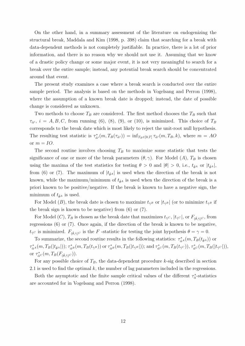
The present study examines a case where a break search is conducted over the entire

sample period. The analysis is based on the methods in Vogelsang and Perron (1998),

where the assumption of a known break date is dropped; instead, the date of possible

change is considered as unknown.

Two methods to choose TB are considered. The first method chooses the TB such that

ταi , i = A, B, C, from running (6), (8), (9), or (10), is minimized. This choice of TB

corresponds to the break date which is most likely to reject the unit-root null hypothesis.

The resulting test statistic is τ ∗αi(m, TB(ταi)) = infTB∈[0,T ] ταi(m,TB, k), where m = AO

or m = IO.

The second routine involves choosing TB to maximize some statistic that tests the

significance of one or more of the break parameters (θ, γ). For Model (A), TB is chosen

using the maxima of the test statistics for testing θ > 0 and |θ| > 0, i.e., tθA or |tθA|,from (6) or (7). The maximum of |tθA| is used when the direction of the break is not

known, while the maximum/minimum of tθA is used when the direction of the break is a

priori known to be positive/negative. If the break is known to have a negative sign, the

minimum of tθA is used.

For Model (B), the break date is chosen to maximize tγB or |tγB | (or to minimize tγB if

the break sign is known to be negative) from (6) or (7).

For Model (C), TB is chosen as the break date that maximizes tγC , |tγC |, or F(θ,γ)C , from

regressions (6) or (7). Once again, if the direction of the break is known to be negative,

tγC is minimized. F(θ,γ)C is the F -statistic for testing the joint hypothesis θ = γ = 0.

To summarize, the second routine results in the following statistics: τ ∗αA(m,TB(tθA)) or

τ ∗αA(m,TB(|tθA|)); τ ∗αB(m,TB(tγB)) or τ ∗αB(m,TB(|tγB |)); and τ ∗αC (m,TB(tγC )), τ ∗αC (m,TB(|tγC |)),or τ ∗αC (m, TB(F(θ,γ)C )).

For any possible choice of TB, the data-dependent procedure k-sig described in section

2.1 is used to find the optimal k, the number of lag parameters included in the regressions.

Both the asymptotic and the finite sample critical values of the different τ ∗α-statistics

are accounted for in Vogelsang and Perron (1998).

12

2.4 Special case 2: Unit-root test allowing for multiple unknown breaks

A model following the Perron methodology, but with multiple breaks, is proposed in

Morimune and Nakagawa (1997). There, the possible breaks are assumed to be exoge-

nously given. Another article dealing with the issue is Bai and Perron (2003), with a

focus on estimation of the break dates and model estimation, rather than tests for a unit

root.

In this paper, the model of choice is instead the one proposed by Lumsdaine and Papell

(1997). It involves a search for the location of two possible breaks in the following model

setting:

(AA) pt = µ + βt + θ1DU1t + θ2DU2t

+αpt−1 +k∑

i=1

ci∆pt−i + et

(CA) pt = µ + βt + θ1DU1t + γDT1t + θ2DU2t (11)

+αpt−1 +k∑

i=1

ci∆pt−i + et

(CC) pt = µ + βt + θ1DU1t + γDT1t + θ2DU2t + γ2DT2t

+αpt−1 +k∑

i=1

ci∆pt−i + et,

where

DUit = 1 if t > TBi, 0 otherwise; and

DTit = t− TBi if t > TBi, 0 otherwise,

where i = AA,CA, or CC. Model (AA) corresponds to Model (A) with two break

dates; Model (CA) corresponds to Model (C) at the first break date and Model (A) at

the second break date; and Model (CC) corresponds to Model (C) with two break dates.

Lumsdaine and Papell compute the limiting distribution of the estimated test statistic

τ ∗αi(TB1, TB2) = infTB1,TB2ταi(TB1, TB2) over distinct pairs of values of (TB1, TB2) for TB1 =

k0, k0+1, ..., T−k0, TB2 = k0, k0+1, ..., T−k0, TB1 6= TB2, TB1 6= (TB2±1). Here, k0 = Tδ0,

and δ0 represents some startup fraction of the sample.

13

3 Data

In this section we give a description of the data set used in the paper. But we begin with

a short overview of the European market for iron ore, closely following Hellmer (1997,

part I).

The world iron-ore market consists of a European and an Asian market. The price

of iron ore is set once a year in negotiations between the major supplier and the major

user in each market. Negotiating parts in the European market are most commonly steel

producers from Germany and the Brazilian iron ore company CVRD. The resulting prices

from the negotiations in each market are taken as the market prices for the coming year,

used by all other exporters of iron ore; thus, the Swedish company LKAB can be seen

as a price-taker and has no influence on the world price. All prices to Europe are set as

f.o.b. prices10, but prices are adjusted so that in principle, all prices to the buyer’s port

are equalized. Usually this means that for the European market, the f.o.b. price in Brazil

is lower than the f.o.b. price in Sweden because of the shipping distance. There are two

predominant qualities of iron ore traded on the world market: sinter feed (also called

fines), and pellets, which earns a premium relative to fines.

The world trade in iron ore was limited before 1940. Trading volumes began to grow

after the second world war, but the most significant increases were during the 1950s and

1960s, when transportation costs fell and more distant iron-ore deposits became profitable

to exploit. Thus if one wants to examine the European or the world market for iron ore,

data from the period before the second world war is not of any great interest.

Our data set consists of prices from Brazil and Sweden, which suits the purpose of

this paper well: Firstly, the data are from a period when world trade was substantial.

Secondly, Brazil is one of the most significant players on the European market, and Sweden

is a significant one.

Prices are expressed in US cents per metric ton 1% Fe-unit, which is equivalent to US

dollars per metric ton pure iron. The data are supplied from the World Bank and from

LKAB and consist of the following time series:

• Brazilian fines, 1960 to 2002 (BR f): Companhia Vale do Rio Doce (CVRD) contract

price for European markets. Itabira sinter feed f.o.b. Tubarao, up to 1986, and

Carajas sinter feed f.o.b. Carajas, thereafter. (source: the World Bank)

• LKAB fines f.o.b. Narvik, 1970 to 2002 (LKAB f N): Luossavaara-Kiirunavaara

Aktiebolag (LKAB) contract price for European markets (source: LKAB)

• LKAB fines f.o.b. Lulea, 1970 to 2002 (LKAB f L) (source: LKAB)

10f.o.b. = free on board: the seller is obliged to ship the ore to the sea port and load it on a vessel, andthe buyer covers the overseas costs.

14

• LKAB pellets f.o.b. Narvik/Lulea, 1970 to 2002 (LKAB p) (source: LKAB), and

• CVRD pellets f.o.b. Tubarao, 1971 to 2002 (CVRD p) (source: LKAB).

Prices are deflated with yearly averages of the Producer Price Index for finished goods

from the U.S. Department of Labor, Bureau of Labor Statistics, with 1982 as base year.

The deflated series are transformed by taking their natural logarithm. Thus, pt = ln(PNt ×

100/PPIt), where PNt are nominal $US-prices and PPIt is the Producer Price Index

(PPI1982 = 100). In the sequel, ’level’ denotes pt and ’first difference’ denotes ∆pt =

pt − pt−1.

4 Results

Following the structure of section 2, we begin with the empirical results from the ADF-

test. After a discussion of the results from the tests with an exogenous structural break,

the outcome of the endogenous-break procedures is commented. The section is closed

with the two-breaks procedure involving a break search.11

Before continuing, some general comments are in place. To begin with, unit-root testing

is a tricky business. Several books have been written on the subject, and among other

things, the question of why we should bother to test for unit root at all is raised. This study

therefore tries to give a motivation of why the issue is important for mineral commodities,

as stated in the introduction.

The main, and perhaps obvious, guideline the author uses for drawing conclusions from

the empirical results, is that a rejection of the unit-root null at a low significance level is

more valuable information than a non-rejection. In other words, a non-rejected null is by

no means regarded as an accepted one. The reason is that for a population autoregressive

parameter lying very close to, but not equal to one, few of the available tests can be relied

on. Instead of concluding that the process has a unit root, a non-rejection of the null can

be seen as either that, or as a sign of a stationary time-series process with a first-order

autoregressive parameter close to one.

Another issue concerns the bootstrap tests performed.12 Obviously, a case where the

result from the asymptotic test coincides with the result from the bootstrap is worth more

than a case where the different types of tests give different results. As will be seen later in

the paper, the bootstrap results often, but not always, agree nicely with the asymptotic

ones.

11All results in the paper were generated using Ox version 3.00.12For a description of the bootstrap routines, see Appendix A.

15

pt = α + ρpt−1 +∑k

j=1 γj∆pt−j + βt + ut ∆pt = θ∆pt−1 + ut

α ρ β θBR f 1.091 0.681 -0.003 0.211

[2.998]1 (-3.028) [-1.890]10 (-5.116)1

LKAB f N 2.198 0.409 -0.013 0.054[3.467]1 (-3.492)10 [-3.084]1 (-5.201)1

LKAB f L 2.265 0.385 -0.011 0.087[3.822]1 (-3.825)2.5 [-3.427]1 (-5.019)1

LKAB p 1.550 0.627 -0.008 0.144[2.710]2.5 (-2.733) [-2.204]5 (-4.729)1

CVRD p 1.439 0.641 -0.006 0.203[2.749]2.5 (-2.762) [-2.154]5 (-4.376)1

[t-value]c/(τ -statistic)c significant at the c% level

Table 2 Dickey-Fuller tests for a unit root in the level and in the first difference withkmax = 4. Critical values at the 0.01, 0.025, 0.05, and 0.1 significance levels: -4.15, -3.80,-3.50, and -3.18. The 0.01 critical value with no trend or intercept is -2.62.

4.1 Augmented Dickey-Fuller test

The test is applied both to each series (equation (1)) and to the first difference of each

series (∆pt = θ∆pt−1 + ut). Using the modified Box-Pierce Q-statistic, the residuals

from the test regressions are checked for serial correlation, and none is found at the 10%

significance level.13 As stated earlier, k is determined using the k-sig routine described

above, with kmax = 4. This represents roughly ten percent of the sample sizes, as in Ng

and Perron (1995), Perron (1989), Lumsdaine and Papell (1997), and in the empirical

part of Perron (1997). If kmax is found to be binding, it is not increased.

The results from the ADF-tests are displayed in Table 2. Starting with the results from

the test on the differenced series it can be seen that in all five cases, the null hypothesis

is rejected at the one percent significance level. The three fines series have the highest

|τ |-values. The bootstrap results from Table 8 (see appendix A) give a similar picture:

p-values close to zero for the three fines series, and between two and three percent for

pellets. Note that for the pellets series, the bootstrap gives higher p-values than what is

suggested by the asymptotic test. Nevertheless, given all test results, it is very unlikely

that any of the differenced series contains a unit root.

The outcome of the test on the level of the series shows a more heterogeneous picture.

First consider the results from the τ -test. Beginning with the Brazilian fines series, neither

the large sample test nor the bootstrap reject the null. The autoregressive coefficient is

estimated at 0.68, a much higher value than for the rest of the fines series. The test value

13The modified Box-Pierce Q-statistic is applicable to the case when the regressors cannot be assumedto be exogenous, as is the case with lagged dependent variables. For details about the statistic, see Hayashi(2000, p. 147). The test is performed for p = 1, 2, .., 15, where p is the order of autocorrelation checkedfor. For instance, for p = 4, the null hypothesis is that the first 4 autocorrelations are simultaneouslyzero, and the alternative is that at least one is different from zero.

16

for the LKAB fines f.o.b. Narvik lies very close to the five percent critical value, confirmed

by the bootstrap size estimate of 0.06. For the f.o.b. Lulea series, we get a rejection at

the 2.5 percent level, and a bootstrap value of 0.03. The estimated trend coefficients are

negative and significant, at the one percent level for the latter two series and at the ten

percent level for Brazilian fines. The test on the two pellets series results in no rejection of

the null at the ten percent level, and the trend coefficient estimate is once again negative.

The Φ3-statistics—in the same series order as in Table 2—are 4.58, 6.10, 7.42, 3.74,

and 3.84. From Dickey and Fuller (1981, Table VI) we see that the critical values are 9.31

(1%), 7.81 (2.5%), 6.73 (5%), and 5.61 (10%) for T = 50. Thus, we reject the null at the

ten percent level for LKAB fines f.o.b. Narvik, and at the five percent level for LKAB

fines f.o.b. Lulea. Table 8 in appendix A for the Φ3-tests reveal estimated p-values of 0.09

and 0.04 for the two series respectively. Thus, the results from applying the Φ3-tests are

close to those from the τ -tests.

To summarize, we can draw the following conclusions from the ADF-test: None of the

differenced series is likely to contain a unit root. Concerning the tests in level, only in

two cases we get rejections of the null, namely for the τ/Φ3-tests at significance levels of

roughly six/nine percent for the LKAB fines f.o.b. Narvik series and three/four percent

for LKAB fines f.o.b. Lulea.

4.2 A single break at a known date

The tests described in section 2.2 are applied to each series. The year for the first oil

crisis is chosen as the time of the instantaneous break, i.e., TB = 1973. This date is

chosen for two reasons: October 1973 brought an oil embargo by the Organization of

Arab Petroleum Exporting Countries, cutting into the supply of oil and elevating prices

to very high levels. This event, known as the Oil Crisis, had an immense impact on the

world economy. Thus, it would be natural to assume that he energy crisis had an effect

on iron ore prices, and we postulate a structural break in 1973.

A second, perhaps more important motivation for the choice, can be seen by examining

the OECD (1975) and OECD (1976) reports. With 1972 as a starting year, there was a

steady increase in activity in the world iron and steel industry. In spite of the slowdown in

general economic activity and the gathering energy crisis, these strong market conditions

continued at least to mid-1974. The demand from steel-using sectors in the industrialized

countries was continuously high. Also, many developing countries with greater purchasing

power because of the higher prices of agricultural products and raw materials, increased

their steel imports considerably. Many of the steel-intensive industries were very active;

the shipbuilding industry was bustling in 1973, and demand for capital goods in most

OECD countries was higher in 1972 and also in 1973 than the years before.

This picture of the iron and steel industry implies a positive price shock around 1973.

17

Indeed, as will be seen in the results below, the estimated shock in the examined iron ore

prices is positive when significant.

For each test regression, the number of lags is determined by the k-sig procedure, with

kmax = 4. Also, for each test, the modified Q-statistic is computed for p = 1, 2, ..., 15,

with no rejections at the ten percent level for any of the series.

The p-values reported in the result tables are calculated using simulated distributions

for ταA and ταC . Critical points for different values of the nuisance parameter λ (the

ratio between the break date and the sample size) are displayed in Table 9. One of the

reasons for not using the critical values reported in Perron (1989, Tables IV.B and VI.B)

is that a direct comparison with the estimated p-values from the bootstrap tests is made

much easier if the whole distribution is available. Another slight improvement is achieved

by using simulated distributions for more exact values of λ. In Perron’s article, critical

values for λ = 0.1, 0.2, . . . , 0.9 are reported, while for the iron ore samples we need values

for λ = 0.0909, 0.1212, and 0.3256. Perhaps the most important gain has to do with the

number of replications used for simulating the distributions of the test statistics: we use

50,000 replications, while Perron uses 5,000. For more details, see appendix B.

Some figures may be helpful before we continue. In Figures 3–7 (see appendix D), the

estimated broken trend functions according to the filtering regressions from the equations

in (7) are shown. The graphs illustrate what the Perron (AO) tests are all about: the data

is filtered by a broken trend function, and the residuals from that equation are tested for

unit root by ADF-techniques, with critical values that correspond to the type of filtering.

Not surprisingly, Model (B) does not fit the data. Therefore, the test results from that

model are omitted in the sequel. We only consider four possible models: Model (A) with

additive or innovation outliers, and Model (C) with additive or innovation outliers.

Before continuing with the results, a note on how to interpret some of the coefficients

might be useful. When we are dealing with additive outliers, θ measures the magnitude

of the instantaneous break in the level of the trend function in Models (A) and (C), while

γ measures the magnitude of the change in the slope of the trend function in Model (C).

For the case of innovation outliers, the same descriptions hold, but now the break is not

instantaneous; instead, the series reacts gradually to the breaks.

The filtering equations for the two models with additive outliers are presented in Table

3, while the results from the asymptotic and bootstrap tests can be found in Tables 4 and

8, respectively. For all series, the estimated coefficients in the filtering equation of Model

(A) are significant, except for the θ-estimate from the two pellets series. Note that the

estimates of θ are all positive, complying with the situation in the iron and steel market

described above. For Brazilian fines, the coefficient estimates from Model (C) are all

significant, but for the rest of the series they generally are not (except for µ). Introducing

the γ-coefficient does not seem to fit other series than the Brazilian fines prices. As was

18

µi βi θi γ

Model (A): pt = µA + βAt + θADUt + pAt

BR f 3.4579 -0.0175 0.3049[123.0160]1 [-9.2015]1 [6.0398]1

LKAB f N 3.6395 -0.0231 0.1716[62.6146]1 [-9.0323]1 [2.2959]5

LKAB f L 3.5467 -0.0207 0.2295[70.4802]1 [-9.3330]1 [3.5480]1

LKAB p 4.1029 -0.0215 0.1379[53.3282]1 [-6.3294]1 [1.3941]

CVRD p 3.9201 -0.0181 0.1455[48.3026]1 [-5.8157]1 [1.4775]

Model (C): pt = µC + βCt + θCDUt + γDTt + pCt

BR f 3.5626 -0.0315 0.1547 0.0155[74.6537]1 [-5.6207]1 [2.0896]5 [2.6275]2

LKAB f N 3.6453 -0.0254 0.1657 0.0023[25.3272]1 [-0.4838] [1.0778] [0.0436]

LKAB f L 3.5276 -0.0130 0.2490 -0.0077[28.3234]1 [-0.2869] [1.8713]10 [-0.1684]

LKAB p 4.0632 -0.0056 0.1783 -0.0159[21.3473]1 [-0.0805] [0.8767] [-0.2285]

CVRD p 4.0025 -0.0593 0.0623 0.0413[18.4255]1 [-0.5897] [0.2757] [0.4101]

[t-value]c significant at the c% level

Table 3 Results from filtering regressions, additive outlier; TB = 1973.

the case in the ADF-setting, both for the (A) and for the (C) model, the estimated trend

is negative when significant.

For the Brazilian iron ore series, the p-values from the asymptotic test for the (A) and

the (C) models are 0.02 and 0.003, respectively. The bootstrap tests give values of 0.03

and 0.006, which are close to the asymptotic ones.

In analogue with the results from the ADF-test, the two pellets series differ from the

rest. Neither series gives any rejection: the asymptotic/bootstrap p-values are 0.63/0.65

(A) and 0.66/0.67 (C) (LKAB pellets); and 0.37/0.21 (A) and 0.39/0.20 (C) (CVRD

pellets). The latter series is the first case thus far when the asymptotic and bootstrap

tests return significantly different p-values, although all well above ten percent.

The two types of fines series from LKAB give two rejections of the null for Model (A).

Using the asymptotic/bootstrap tests, the p-values are 0.08/0.07 for the f.o.b. Narvik

series, and somewhat lower for the f.o.b. Lulea fines lying at 0.02/0.02. The results

from applying the Model (C) tests are similar with 0.09/0.04 and 0.03/0.01. As in with

CVRD pellets above, the bootstrap tests give significantly lower p-value estimate than

the asymptotic tests.

Now let us turn to the case with innovational outliers displayed in Tables 5 (the test

19

k α σα τα p-valueModel (A):BR f 1 0.381 0.151 -4.099 0.023LKAB f N 1 0.464 0.152 -3.534 0.076LKAB f L 1 0.369 0.155 -4.066 0.021LKAB p 0 0.736 0.123 -2.151 0.629CVRD p 1 0.678 0.123 -2.619 0.365Model (C):BR f 1 0.184 0.158 -5.150 0.003LKAB f N 1 0.464 0.151 -3.541 0.091LKAB f L 1 0.371 0.156 -4.029 0.029LKAB p 0 0.738 0.123 -2.127 0.663CVRD p 1 0.679 0.123 -2.601 0.389

Table 4 Unit-root tests allowing for a single exogenous break, additive outlier, with kmax =4. Test equation: (8) with TB = 1973. For critical values see Table 9.

equations), 6 (the test results), and 8 (bootstrap τ - and F -tests). As with AO, the test

equations of Model (A) generally give coefficient estimates that are significant, while the

ones of from Model (C) are not completely so. Note also that the only significant estimate

of θ in Model (C) is positive, complying with the economic intuition. Furthermore, the

pellets series once again differ from the rest: the coefficient estimates of θ from Model (A)

are not significant for those series, while they are significant for the rest.

Let us begin with the results of the τ -tests. For Brazilian ore, we get rejections at

the one percent level for both Models (A) and (C), and both from the asymptotic and

from the bootstrap tests, with all estimated p-values close to zero. Applying the tests to

LKAB fines f.o.b. Lulea also results in rejections of the null hypotheses. The outcome

of the test for the f.o.b. Narvik series gives higher p-values, and the bootstrap tests give

lower p-values than the asymptotic ones, the difference being largest for Model (C). Also

with innovation outliers the pellets series stand out, with none of the tests giving any

rejections.

Recall that the article by Perron does not give any F -tests of joint hypotheses; thus,

our paper relies solely on bootstrap tests for the Models (A) and (C) with innovational

outliers, as displayed in Table 8. For Model (C) IO, the estimated p-values are close to

those from the τ -tests. For Model (A) IO, all F -tests give p-values that are higher than

the corresponding τ -tests. But the only important difference concerns LKAB fines f.o.b.

Narvik: for that series, with an F -test, we are able to reject the null at the ten percent

level, while with a τ -test, we get a rejection at the five percent level. To summarize, the

F -tests give approximately the same results as the τ -tests. Notice, though, that we have

only used bootstrap methods to perform the first-mentioned.

20

µi βi θi γ di a k

Model (A): pt = µA + βAt + θADUt + dAD(TB)t + aApt−1 +∑k

i=1 ci∆pt−i + et

BR f 2.1258 -0.0115 0.2172 -0.1014 0.3837 1[5.2191]1 [-4.7119]1 [4.3148]1 [-1.2460]

LKAB f N 2.1745 -0.0137 0.1447 0.1547 0.3889 1[3.5052]1 [-3.0992]1 [1.8152]10 [1.4259]

LKAB f L 2.6167 -0.0153 0.1949 0.0640 0.2555 1[4.3698]1 [-3.9431]1 [2.6269]2 [0.6557]

LKAB p 1.4464 -0.0069 0.0631 0.2258 0.6377 1[2.6233]2 [-1.8571]10 [0.7343] [2.0111]10

CVRD p 1.3407 -0.0065 0.1095 0.0782 0.6422 1[2.4846]2 [-1.9808]10 [1.0560] [0.7448]

Model (C): pt = µC + βCt + θCDUt + γCDTt + dCD(TB)t + aCpt−1 +∑k

i=1 ci∆pt−i + et

BR f 2.5022 -0.0231 0.1265 0.0112 -0.1164 0.3007 1[5.7317]1 [-3.6115]1 [1.8881]10 [1.9552]10 [-1.4808]

LKAB f N 2.7927 -0.2152 -0.5666 0.2020 0.1587 0.4129 1[3.8832]1 [-1.6824] [-1.2371] [1.5758] [1.5053]

LKAB f L 3.1677 -0.2030 -0.4706 0.1883 0.0728 0.2854 1[4.7778]1 [-1.8302]10 [-1.1779] [1.6931] [0.7719]

LKAB p 1.9109 -0.1490 -0.4368 0.1423 0.2271 0.6459 1[2.6306]2 [-1.0304] [-0.8469] [0.9830] [2.0206]10

CVRD p 1.1377 -0.0638 -0.0646 0.0587 0.0619 0.7352 0[1.7524]10 [-0.4465] [-0.1759] [0.4108] [0.5550]

[t-value]c significant at the c% level

Table 5 Results from unit-root test regressions, specifications with innovational outliers;TB = 1973 and kmax = 4.

4.3 Special case 1: A single break at an unknown date

Ideally, a researcher with an idea of when a break should occur would like the search

procedure to pick out that particular date, or any date close to it. The results for Brazilian

iron ore displayed in Table 10 are quite satisfactory in that respect:14 All procedures

resulting in a rejection of the null hypothesis at the 2.5 or five percent level pick out 1972

(in one out of six cases) or 1973 as the break date. In the exogenous tests 1973 is selected

as the date of the break, but the year before in the IO-setting, as is the case here, can

also be justified. A gradual change starting in 1972 is not implausible if one consults the

OECD reports mentioned earlier.

Unfortunately, none of the results for the rest of the series is easy to interpret. For

LKAB fines f.o.b. Narvik we get quite many rejections with the years 1980–1982 as break

dates, and some with a break in 1987; and for LKAB fines f.o.b. Lulea we get three

rejections at the ten percent level, with 1972, 1980, and 1982 as break dates (see Tables

11 and 12). The search on LKAB pellets in Table 13 results in some rejections, some of

14Tables 10–14 can be found on pp. 35–37.

21

k α σα τα p-valueModel (A):BR f 1 0.384 0.117 -5.265 0.001LKAB f N 1 0.389 0.166 -3.672 0.056LKAB f L 1 0.256 0.166 -4.494 0.006LKAB p 1 0.638 0.132 -2.749 0.324CVRD p 1 0.642 0.134 -2.675 0.339Model (C):BR f 1 0.301 0.120 -5.811 0.0004LKAB f N 1 0.413 0.162 -3.615 0.078LKAB f L 1 0.285 0.161 -4.445 0.009LKAB p 1 0.646 0.132 -2.680 0.383CVRD p 0 0.735 0.134 -1.969 0.711

Table 6 Unit-root tests allowing for a single exogenous break, innovational outlier, withkmax = 4. Test equations: (6) with TB = 1973. For critical values see Table 9.

the dates being around 1980, and some in 1988. Finally, as can be seen in Table 14, the

procedure chooses dates close to 1980 when rejections occur for CVRD pellets.

Naturally, even for dates far from 1973, the rejections of the null above are valid in

the statistical sense, but it is beyond the scope of this paper to try to find the economic

intuition behind the break dates. It is possible that either the second oil crisis, or the

world recession in the beginning of the 1980s, is responsible for a break in the series.

4.4 Special case 2: Two breaks at unknown dates

The results from the test can be found in Table 7, and for Brazilian fines they are not

very convincing: we get one rejection of the null at the ten percent level. The model

giving the rejection is AA; one of the breaks is found to be in 1974 and the second in

1989. Models CA for Narvik fines and CC for Lulea fines choose 1973 and 1989 as the

break dates (with rejections at the 2.5 percent level). For both Swedish fines series we

get rejections using each type of model at a maximum significance level of ten percent.

Both pellets series behave similarly, with rejections for model AA (with 1980 and 1982

as dates), and for model CA (1988 and 1982).

One interesting feature of the results above is that dates around 1980/1982 are often

chosen as one of the break dates in rejections at significance level five percent or less. The

reasons why a break is postulated in 1973 is given earlier in this paper. Concerning a

possible break soon after 1980 one reason might be the global recession around that date,

although a more thorough investigation is left for future research.

5 Conclusions

Using unit-root tests allowing for an exogenous structural break, the null hypothesis of a

unit root is rejected for Brazilian fines and LKAB fines f.o.b. Lulea. It is interesting to

22

Test resultsi TB1(ταi) TB2(ταi) k τ∗αi(TB1, TB2)

BR fAA 1989 1974 1 -6.08910%

CC 1982 1973 1 -6.298CA 1973 1982 1 -6.296

LKAB f NAA 1982 1973 1 -6.08910%

CC 1986 1992 4 -7.1622.5%

CA 1989 1973 1 -7.0992.5%

LKAB f LAA 1982 1973 1 -7.0021%

CC 1973 1989 1 -7.0572.5%

CA 1973 1982 1 -7.1682.5%

LKAB pAA 1980 1982 3 -7.1911%

CC 1987 1973 1 -6.174CA 1988 1982 3 -7.1422.5%

CVRD pAA 1980 1982 3 -6.8622.5%

CC 1987 1974 1 -5.715CA 1988 1982 3 -7.3411%

Critical values‡

i 1% 2.5% 5% 10%AA -6.94 -6.53 -6.24 -5.96CC -7.34 -7.02 -6.82 -6.49CA -7.24 -7.02 -6.65 -6.33

‡Source: Lumsdaine and Papell (1997). τ∗αi (·)c% signifi-

cant at the c% level.

Table 7 Unit-root tests involving a search for two breaks, kmax = 4.

note that the LKAB fines f.o.b. Narvik series gives rejections at higher significance levels

than the f.o.b. Lulea series. The two pellets series stand out, since none of the exogenous-

break test equations seems to fit the data, and we get no rejections of the null. This is

an interesting result, since the price formation should in theory give the same properties

for pellets as for fines.

If all models with exogenous trend breaks are to be summarized, the model of choice

for the three fines series would be Model (A) from Perron (1989), either with additive or

with innovational outliers. That model assumes a break in the level, but no change in the

slope of the trend function. With innovational outliers the break is not instantaneous;

instead, the series reacts gradually to a structural change.

The results from the tests with endogenous break(s) are more difficult to interpret,

except for Brazilian fines with one break, where we get many rejections of the null involving

breaks in 1973 (the first oil crisis). For the rest of the series, a number of rejections occur

around 1980–1982 (the world recession following the second oil embargo), but also other

break dates are estimated. The routine involving a search for one break must be handled

with care: depending on the criteria used, we may get different break dates. The search

23

routine involving two breaks gives quite many rejections of the null hypothesis, but in

many cases it is difficult to give an economic explanation for the break dates chosen.

To summarize the empirical findings, a time-series analysis of the five iron-ore prices

must take into consideration the structural break that seems to have taken place during

the first half of the 1970s. The state of the steel and iron ore industry seems to have

caused a structural break in three of the five examined series. Evidently, it is possible

that neglecting the break, as is done in the simple ADF-test, results in a false non-rejection

of the unit-root null hypothesis. This is the case for Brazilian fines. For LKAB fines f.o.b.

Narvik and Lulea, we get a rejection of the null hypothesis also by using the ADF-test,

but the estimated first autoregressive coefficient is too high when the break is neglected.

Finally, more accurate critical values for Models (A) and (C) with an exogenous break

are given and used, compared to the ones reported in Perron (1989). Instead of relying on

5,000 replications to simulate the distributions of the test statistics, we use 50,000. Perron

(1989, p. 1377) suggests that the limiting distributions are symmetric around λ = 0.5.

This is more clearly seen with 50,000 than with 5,000 replications.

References

Abadir, K., and W. Distaso (2003): “Testing joint hypotheses when one of the alter-natives is one-sided,” unpublished.

Agbeyegbe, T. D. (1993): The Stochastic Behavior of Mineral-CommodityPriceschap. 21, pp. 339–353, in (Peter C. B. Phillips, (ed.) 1993).

Ahrens, W. A., and V. R. Sharma (1997): “Trends in Natural Resource Commod-ity Prices: Deterministic or Stochastic?,” Journal of Environmental Economics andManagement, 33, 59–74.

Bai, J., and P. Perron (2003): “Computation and Analysis of Multiple StructuralChange Models,” Journal of Applied Econometrics, 18, 1–22.

Christiano, L. J. (1992): “Searching for a Break in GNP,” Journal of Business andEconomic Statistics, 3, 237–250.

Davison, A. C., and D. V. Hinkley (1997): Bootstrap Methods and their Applications.Cambridge University Press, Cambridge, UK.

Dickey, D. A., and W. A. Fuller (1981): “Likelihood Ratio Statistics for Autore-gressive Time Series with a Unit Root,” Econometrica, 49, 1057–1072.

Hamilton, J. D. (1994): Time Series Analysis. Princeton University Press, Princeton,New Jersey.

Hayashi, F. (2000): Econometrics. Princeton University Press, Princeton, New Jersey.

Hellmer, S. (1997): “Competitive Strength in Iron Ore Production,” Ph.D. thesis,Lulea University of Technology.

24

Howie, P. (2002): “Time-Series Models Analyzing the Long-Term Behaviour of MineralPrices,” working paper from the University of Montana.

Leon, J., and R. Soto (1997): “Structural Breaks and Long-Run Trends in CommodityPrices,” Journal of International Development, 9, 347–366.

Lumsdaine, R. L., and D. H. Papell (1997): “Multiple Trend Breaks and the Unit-Root Hypothesis,” The Review of Economics and Statistics, 79, 212–218.

Maddala, G. S., and I.-M. Kim (1998): Unit Roots, Cointegration, and StructuralChange. Cambridge University Press, Cambridge, UK.

Metcalf, G. E., and K. A. Hassett (1995): “Investment Under Alternative ReturnAssumptions: Comparing Random Walks and Mean Reversion,” Journal of EconomicDynamics and Control, 19, 1471–1488.

Morimune, K., and M. Nakagawa (1997): “Unit Root Tests Which Allow for MultipleTrend Breaks,” Discussion Paper No. 457, Kyoto Institute of Economic Research, KyotoUniversity, Japan.

Nelson, C. R., and C. I. Plosser (1982): “Trends and Random Walks in Macroeco-nomic Time Series: Some Evidence and Implications,” Journal of Monetary Economics,10, 139–162.

Ng, S., and P. Perron (1995): “Unit Root Tests in ARMA Models with Data-Dependent Methods for the Selection of the Truncation Lag,” Journal of the AmericanStatistical Association, 90, 268–281.

OECD (1975): “The Iron and Steel Industry in 1973 and Trends in 1974,” .

(1976): “The Iron and Steel Industry in 1974 and Trends in 1975,” .

Perron, P. (1989): “The Great Crash, the Oil Price Shock, and the Unit Root Hypoth-esis,” Econometrica, 57, 1361–1401.

(1997): “Further Evidence on Breaking Trend Functions in MacroeconomicVariables,” Journal of Econometrics, 80, 355–385.

Perron, P., and T. J. Vogelsang (1992): “Testing for a Unit Root in a TimeSeries with a Changing Mean: Corrections and Extensions,” Journal of Business andEconomic Statistics, pp. 467–470.

(1993): “Erratum: The Great Crash, the Oil Price Shock, and the Unit RootHypothesis,” Econometrica, 61, 248–249.

Peter C. B. Phillips, (ed.) (1993): Models, Methods, and Applications of Econo-metrics: Essays in Honor of A. R. Bergstrom. Blackwell Publishers, Cambridge, Mas-sachusetts.

Sarkar, S. (2003): “The Effect of Mean Reversion on Investment Under Uncertainty,”Journal of Economic Dynamics and Control, 28, 377–396.

25

Schwartz, E. S. (1997): “The Stochastic Behavior of Commodity Prices: Implicationsfor Valuation and Hedging,” Journal of Finance, 52, 923–973.

Slade, M. E. (1982): “Trends in Natural-Resource Commodity Prices: An Analysis ofthe Time Domain,” Journal of Environmental Economics and Management, 9, 122–137.

Vogelsang, T. J., and P. Perron (1998): “Additional Tests for a Unit Root Allowingfor a Break in the Trend Function at an Unknown Date,” International EconomicReview, 39, 1073–1100.

Zivot, E., and D. W. K. Andrews (1992): “Further Evidence on the Great Crash, theOil-Price Shock, and the Unit-Root Hypothesis,” Journal of Business and EconomicStatistics, 3, 251–270.

A Bootstrap procedures

ADF, level ADF, diff (A) AO (A) IO (C) AO (C) IOTests using τ -statisticsBR f 0.138 0.002 0.032 0.002 0.006 0.001LKAB f N 0.061 0.001 0.069 0.048 0.042 0.049LKAB f L 0.030 0.001 0.021 0.009 0.012 0.009LKAB p 0.238 0.023 0.655 0.248 0.667 0.252CVRD p 0.226 0.028 0.211 0.262 0.202Tests using F/Φ3-statisticsBR f 0.202 0.003 0.003LKAB f N 0.086 0.095 0.047LKAB f L 0.041 0.024 0.008LKAB p 0.330 0.449 0.351CVRD p 0.313 0.449

Table 8 Empirical size from bootstrap tests, 50,000 replications. The first two columnscorrespond to an ADF-test in level or first difference. The rest can be read as follows: forinstance, (A) AO is Model (A) with an additive outlier from Perron (1989). The numberof lags is the same as in the corresponding asymptotic tests presented earlier in the paper,TB = 1973 where applicable. For detailed information on the bootstrap procedures, see thecorresponding appendix.

In this section, the bootstrap procedures used in the paper are described. Two differentclasses of tests are used: bootstrap tests based on τ - or F -statistics. For each series, fivedifferent bootstrap versions of various asymptotic τ -tests are applied: the ADF-test withboth a constant and a trend; the Model (A) Perron test with additive (AO) and innovationoutliers (IO); and the Model (C) Perron test with AO and IO. In addition, the ADF-testwith no constant or trend is applied to each differenced series.

Three bootstraps based on F -statistics are applied to each series: the ADF-test withboth a constant and a trend, the Model (A) Perron test with innovation outliers (IO),and the Model (C) Perron test with IO.

The results from the various bootstrap tests are displayed in Table 8. The number ofreplications R is set to 50,000 in each bootstrap.

26

A.1 Bootstrap Dickey-Fuller test with a constant, no trend, and k = 0(τ-test)

This test is only applied to the difference of the series; for simplicity, we write ’pt’ instead of’∆pt’. The example in Davison and Hinkley (1997, pp. 391–393) and the recommendationsin Maddala and Kim (1998, ch. 10) are followed, and the test involves the following steps:

1. Using the sample {p1}T1 , estimate the model

pt = α + ρpt−1 + ut (12)

by OLS and construct the test statistic τ = (ρ − 1)/σρ, where σρ is the estimatedstandard error of ρ. The null hypothesis is ρ = 1, while the alternative is ρ < 1.

2. Construct T − 1 residuals et under H0,

et = ∆pt = α + ut.

3. Create R bootstrap samples by sampling with replacement and with equal proba-bility from {et}T

2 to obtain simulated innovations {e∗t}T2 .

4. For each bootstrap sample r = 1, 2, ..., R, create a {p∗t} sequence using recursion:set p∗1 = p1, and then

p∗t = p∗t−1 + e∗t , t = 2, 3, ..., T.

5. For each r, run the regression

p∗t = α∗ + ρ∗p∗t−1 + ut,

where t = 2, 3, ..., T , and calculate the test statistic τ ∗ = (ρ∗ − 1)/σρ∗ .

6. Estimate the size of the test by(PR

r=1 Ir)+1

R+1, where Ir = 1 if τ ∗ < τ and Ir = 0

otherwise.

As is evident from above, no centering of the residuals is performed, and that applies toall results in Table 8. In a preliminary study, all results were calculated with or withoutcentering for R = 1, 000, and the differences obtained were insignificant. Thus centeringthe residuals is not expected to change the results.

A.2 Bootstrap Dickey-Fuller test with trend and k > 0 (τ-test)

1. Estimate the regression

∆pt = α + δpt−1 + βt +k∑

j=1

γj∆pt−j + et, (13)

by OLS and construct the test statistic τδ = δ/σδ. The null hypothesis is δ = 0,and the alternative is δ < 0.

27

2. Generate residuals from (13) under H0, i.e.,

et = ∆pt − α− βt−k∑

j=1

γj∆pt−j,

where the coefficients are estimated with H0 imposed, i.e., from running (13) withoutpt−1 as regressor.

3. Create R bootstrap samples by sampling with replacement and with equal proba-bility from {et}T

k+2 to obtain simulated innovations {e∗t}Tk+2.

4. For each bootstrap sample r = 1, 2, ..., R, create the sequences {∆p∗t} and {p∗t}: set∆p∗t = ∆pt and p∗t = pt for t = 2, 3, ..., k + 1, and use the recursive equations

∆p∗t = α + βt +k∑

j=1

γj∆p∗t−j + e∗t and

p∗t = ∆p∗t + p∗t−1

for t = k + 2, 3, ..., T . Calculate the test statistic τδ∗ = δ∗/σδ∗ using step (1).

5. Estimate the size of the test by (1 +∑R

r=1 Ir)/(1 + R), where Ir = 1 if τδ∗ < τδ andIr = 0 otherwise.

A.3 Bootstrap Perron test of Model (A) with additive outliers (τ-test)

The description of the bootstrap for Model (C) is omitted due to its similarity: the onlydifference is the inclusion of one more dummy regressor.

1. Run the regression

pt = µA + βAt + θADUt + pt

to obtain the OLS-estimates (µA, βA, θA).

2. Estimate the model

pt = αpt−1 +k∑

j=0

ωjD(TB)t−j +k∑

j=1

cj∆pt−j + ut (14)

by OLS and construct the test statistic τα = (α − 1)/σα. The null hypothesis isα = 1, while the alternative is α < 1.

3. Generate residuals from (14) under H0,

ut = ∆pt −k∑

j=0

ωjD(TB)t−j −k∑

j=1

cj∆pt−j,

28

where ωj and cj are estimated with H0 imposed.

4. Create R bootstrap samples by sampling with replacement and with equal proba-bility from {ut}T

k+2 to obtain simulated innovations {u∗t}Tk+2.

5. For each bootstrap sample r = 1, 2, ..., R, create {∆p∗t} and {p∗t} sequences usingrecursion: set ∆p∗t = ∆pt and p∗t = pt for t = 2, 3, ..., k + 1, and use the recursiveequations

∆p∗t =k∑

j=0

ωjD(TB)t−j +k∑

j=1

cj∆p∗t−j + u∗t and

p∗t = ∆p∗t + p∗t−1

for t = k + 2, 3, ..., T .

6. For each r, create

p∗t = µA + βAt + θADUt + p∗t ,

where t = 2, 3, ..., T , and calculate the test statistic τα∗ = (α∗ − 1)/σα∗ using steps(1) and (2) above.

7. Estimate the size of the test by (1 +∑R

r=1 Ir)/(1 + R), where Ir = 1 if τα∗ < τα andIr = 0 otherwise.

A.4 Bootstrap Perron test of Model (A) with innovation outliers (τ-test)

The description of the bootstrap for Model (C) is omitted due to its similarity.

1. Estimate the regression

∆pt = µA + βAt + θADUt + dAD(TB)t + δpt−1 +k∑

i=1

cAi ∆pt−i + et (15)

by OLS and construct the test statistic τδ = δ/σδ. The null hypothesis is δ = 0,and the alternative is δ < 0.

2. Generate residuals from (15) under H0, i.e.,

et = ∆pt − µA − βAt− θADUt − dAD(TB)t −k∑

i=1

cAi ∆pt−i,

where the coefficients are estimated with H0 imposed, i.e., from running (15) withno pt−1 on the right hand side.

3. Create R bootstrap samples by sampling with replacement and with equal proba-bility from {et}T

k+2 to obtain simulated innovations {e∗t}Tk+2.

29

4. For each bootstrap sample r = 1, 2, ..., R, create the sequences {∆p∗t} and {p∗t}: set∆p∗t = ∆pt and p∗t = pt for t = 2, 3, ..., k + 1, and then for t = k + 2, 3, ..., T , use therecursive equations

∆p∗t = µA + βAt + θADUt + dAD(TB)t +k∑

i=1

cAi ∆p∗t−i + e∗t and

p∗t = ∆p∗t + p∗t−1.

Calculate the test statistic τδ∗ = δ∗/σδ∗ using step (1).

5. Estimate the size of the test by (1 +∑R

r=1 Ir)/(1 + R), where Ir = 1 if τδ∗ < τδ andIr = 0 otherwise.

A.5 Bootstrap Dickey-Fuller test with trend and k > 0 (Φ3-test)

The F -statistic below corresponds to the Φ3-statistic from Dickey and Fuller (1981). Fromthe F -statistics class, only this procedure is shown, since the A (IO) and C (IO) versionsare similar. (To perform the structural-break bootstraps, simply add the relevant dummyvariables to the regressions.)

1. Estimate the regression

∆pt = α + δpt−1 + βt +k∑

j=1

γj∆pt−j + et, (16)

by OLS and construct the test statistic F(δ,β) = (Rb− q)′[s2R(X′X)−1R′]−1(Rb− q)/2,where

R2×(3+k)

=

(0 1 0 0 · · · 00 0 1 0 · · · 0

),

b(3+k)×1

= (α δ β c1 · · · ck)′, q

2×1= 0,

XT×(3+k)

= (x1 x2 · · · xT )′, s2 = e′e/(T − 3− k),

eT×1

= (e1 e2 · · · eT )′, and

xt(3+k)×1

= (1 pt−1 t ∆pt−1 · · · ∆pt−k)′.

F(δ,β) is used to test H0 : θ = 0 against H0 : θ 6= 0, where θ = (δ β)′.

2. Generate residuals from (16) under H0, i.e.,

30

et = ∆pt − α−k∑

j=1

γj∆pt−j,

where the coefficients are estimated with H0 imposed, i.e., from running (16) withoutpt−1 and t as regressors.

3. Create R bootstrap samples by sampling with replacement and with equal proba-bility from {et}T

k+2 to obtain simulated innovations {e∗t}Tk+2.

4. For each bootstrap sample r = 1, 2, ..., R, create the sequences {∆p∗t} and {p∗t}: set∆p∗t = ∆pt and p∗t = pt for t = 2, 3, ..., k + 1, and use the recursive equations

∆p∗t = α +k∑

j=1

γj∆p∗t−j + e∗t and

p∗t = ∆p∗t + p∗t−1

for t = k + 2, 3, ..., T . Calculate the test statistic F(δ∗,β∗) using step 1.

5. Estimate the size of the test by (1+∑R

r=1 Ir)/(1+R), where Ir = 1 if F(δ∗,β∗) > F(δ,β)

and Ir = 0 otherwise.

B Simulated distributions for τα

Assume that W (t) is a standard Wiener process. In order to simulate the distributionsof the test statistics ταi , i = A,C, from Theorem 2 in Perron (1989, p. 1373) the follow-

ing functions of W (t) need to be approximated: W (1), W (λ),∫ λ

0W (r)dr,

∫ λ

0rW (r)dr,∫ 1

λW (r)dr,

∫ 1

λrW (r)dr,

∫ 1

0W (r)dr,

∫ 1

0rW (r)dr, and

∫ 1

0W (r)2dr. Below we show how

these functions are approximated and the expressions are accompanied by (very) informalproofs.

Let {et}Tt=1 be a sequence of pseudo-random i.i.d. N(0, 1) variables. Let ’

L−→’ denote

convergence in distribution, and ’d=’ equality in distribution. Then for λ ∈ [0, 1] and

xt =∑t

i=1 ei we get:

1.T− 1

2 xTd= W (1) ∼ N(0, 1)

Proof: Being a sum of normally distributed variables, the expression is normallydistributed with mean zero and variance

Var(T− 12 xT ) = T−1Var(xT )

= T−1T = 1.

2.T− 1

2 x[λT ]L−→ W (λ) ∼ N(0, λ),

31

where [·] denotes the integer-part function.

Proof: Obviously, T− 12 x[λT ] is normally distributed with mean zero and with variance

Var(T− 12 x[λT ]) = T−1Var(x[λT ]) = T−1[λT ]

L−→ λ.

3.

T− 32

[λT ]∑t=1

xtL−→

∫ λ

0

W (r)dr.

Proof: We have

T− 12 xt = W (

t

T), (17)

which can be proved in a similar manner as 1. above. Then we can write

T− 32

[λT ]∑t=1

xt =

[λT ]∑t=1

T− 12 xt

t− (t− 1)

T=

[λT ]∑t=1

T− 12 xt∆(

t

T)

d=

[λT ]∑t=1

W (t

T)(∆

t

T)

L−→∫ λ

0

W (r)dr,

where r ≡ tT.

Equation (17) and the last identity are used in the proofs of 4–6 and of 9 below.

4.

T− 52

[λT ]∑t=1

txtL−→

∫ λ

0

rW (r)dr.

Proof:

T− 52

[λT ]∑t=1

txt =

[λT ]∑t=1

(t

T)T− 1

2 xt∆(t

T)

d=

[λT ]∑t=1

(t

T)W (

t

T)∆(

t

T)

L−→∫ λ

0

rW (r)dr.

5.

T− 32

T∑

t=[λT ]

xtL−→

∫ 1

λ

W (r)dr.

Proof:

32

T− 32

T∑

t=[λT ]

xt =T∑

t=[λT ]

T− 12 xt∆(

t

T)

d=

T∑

t=[λT ]

W (t

T)∆(

t

T)

L−→∫ 1

λ

W (r)dr,

6.

T− 52

T∑

t=[λT ]

txtL−→

∫ 1

λ

rW (r)dr.

Proof:

T− 52

T∑

t=[λT ]

txt =T∑

t=[λT ]

(t

T)T− 1

2 xt∆t

T

d=

T∑

t=[λT ]

(t

T)W (

t

T)∆

t

T

L−→∫ 1

λ

rW (r)dr.

7.

T− 32

T∑t=1

xtL−→

∫ 1

0

W (r)dr.

Proof: This is 3 with λ = 1.

8.

T− 52

T∑t=1

txtL−→

∫ 1

0

rW (r)dr.

Proof: This is 4 with λ = 1.

9.

T−2

T∑t=1

x2t

d=

∫ 1

0

W (r)2dr.

Proof:

T−2

T∑t=1

x2t =

T∑t=1

(T− 12 xt)(T

− 12 xt)∆(

t

T)

d=

∫ 1

0

W (r)2dr.

Following Perron, for {et}1,000t=1 , the sums 1–9 are used to calculate one simulated value

of ταA or ταC . The latter is done with the help of the expressions in Perron (1989,pp. 1373–1374). (Note that there are several misprints, as pointed out in Perron andVogelsang (1993).) This is replicated 5,000 times, thereby simulating the distributions of

33

the statistics. For illustration, the density functions for λ = 0.3256 are plotted in Figure1. This break ratio corresponds to the Brazilian fines sample range with TB = 1973,while for the CVRD pellets sample we have λ = 0.0909, and for the rest of the series,λ = 0.1212.

−5.5 −5.0 −4.5 −4.0 −3.5 −3.0 −2.5 −2.0 −1.5 −1.0 −0.5 0.0 0.5 1.0 1.5

0.1

0.2

0.3

0.4

0.5ταA

−6.5 −6.0 −5.5 −5.0 −4.5 −4.0 −3.5 −3.0 −2.5 −2.0 −1.5 −1.0 −0.5 0.0 0.5 1.0

0.1

0.2

0.3

0.4

0.5 ταC

Figure 1 Simulated distributions of ταA and ταC using 5,000 replications and λ = 0.3256.

A comparison with the percentage points in Perron (1989, Tables IV.B and VI.B) revealssome slight differences. In order to see how robust the results from the simulation arewith T = 1, 000 and number of replications R = 5, 000, the experiment is repeated once.The difference between the first and the second simulation (as measured by the sum ofsquared differences between corresponding quartiles) is of the same order as the differencebetween any of them and Perron’s critical tables, and can thus be attributed to chance.

In order to increase the reliability of the critical values, a simulation with R = 50, 000 isperformed twice; since the differences between quartiles from the two sets of simulationsis much smaller than for R = 5, 000, in this paper we use 50,000 replications.

The percentage points of the simulated distributions of ταA and ταC are displayed inTable 9, and the new simulated distributions are plotted in Figure 2.

−6.0 −5.5 −5.0 −4.5 −4.0 −3.5 −3.0 −2.5 −2.0 −1.5 −1.0 −0.5 0.0 0.5 1.0 1.5

0.1

0.2

0.3

0.4

0.5ταA

−6.0 −5.5 −5.0 −4.5 −4.0 −3.5 −3.0 −2.5 −2.0 −1.5 −1.0 −0.5 0.0 0.5 1.0 1.5

0.1

0.2

0.3

0.4

0.5ταC

Figure 2 Simulated distributions of ταA and ταC using 50,000 replications and λ = 0.3256.

34

λ = 0.09 0.1 0.12 0.2 0.3 0.33 0.4 0.5 0.6 0.7 0.8 0.9ταA

1% -4.29 -4.28 -4.33 -4.36 -4.38 -4.41 -4.35 -4.34 -4.36 -4.37 -4.38 -4.272.5% -3.95 -3.96 -3.98 -4.04 -4.05 -4.06 -4.04 -4.02 -4.04 -4.05 -4.05 -3.955% -3.67 -3.69 -3.72 -3.79 -3.79 -3.78 -3.77 -3.75 -3.77 -3.79 -3.79 -3.6910% -3.37 -3.39 -3.41 -3.49 -3.49 -3.48 -3.47 -3.45 -3.46 -3.49 -3.49 -3.3990% -1.39 -1.39 -1.42 -1.46 -1.39 -1.37 -1.28 -1.22 -1.27 -1.40 -1.47 -1.3995% -1.09 -1.07 -1.11 -1.16 -1.06 -1.04 -0.93 -0.85 -0.91 -1.08 -1.16 -1.0797.5% -0.81 -0.79 -0.82 -0.87 -0.77 -0.77 -0.63 -0.52 -0.61 -0.78 -0.88 -0.7899% -0.46 -0.48 -0.49 -0.53 -0.44 -0.41 -0.27 -0.13 -0.24 -0.43 -0.55 -0.44

ταC

1% -4.33 -4.35 -4.43 -4.59 -4.69 -4.76 -4.81 -4.81 -4.80 -4.73 -4.60 -4.342.5% -4.01 -4.02 -4.08 -4.27 -4.38 -4.43 -4.48 -4.49 -4.48 -4.39 -4.28 -4.015% -3.72 -3.75 -3.80 -3.99 -4.12 -4.16 -4.21 -4.23 -4.22 -4.12 -3.99 -3.7510% -3.41 -3.43 -3.50 -3.68 -3.83 -3.86 -3.91 -3.94 -3.92 -3.82 -3.68 -3.4390% -1.41 -1.41 -1.46 -1.61 -1.77 -1.81 -1.91 -1.96 -1.90 -1.77 -1.60 -1.4195% -1.09 -1.09 -1.13 -1.29 -1.45 -1.49 -1.59 -1.65 -1.59 -1.44 -1.28 -1.0997.5% -0.81 -0.80 -0.85 -0.99 -1.14 -1.20 -1.31 -1.39 -1.30 -1.15 -0.99 -0.7999% -0.46 -0.49 -0.50 -0.64 -0.80 -0.90 -0.98 -1.07 -0.97 -0.82 -0.62 -0.46

Table 9 Percentage points of the simulated distributions of ταA and ταC , 50,000 replica-tions.

C Results from search for one break

Test results Critical values‡

i m TB(s) s k τ∗αi(m,TB(s)) 1% 2.5% 5% 10%A AO 1977 −ταi 1 -4.5062 −5.92 −5.49 −5.20 −4.83A IO 1972 −ταi 1 -5.44095% −5.92 −5.58 −5.23 −4.92C AO 1973 −ταi 1 -5.1505 −6.17 −5.87 −5.56 −5.21C IO 1973 −ταi 1 -5.81145% −6.32 −5.90 −5.59 −5.29A AO 1974 tθi 0 -4.1345 −5.24 −4.86 −4.53 −4.14A IO 1973 tθi 1 -5.26545% −5.70 −5.21 −4.92 −4.53A AO 1974 t|θi| 0 -4.1345 −5.35 −4.95 −4.73 −4.34A IO 1973 t|θi| 1 -5.2654 −5.85 −5.51 −5.18 −4.83C AO 1980 −tγi 1 -3.9648 −5.62 −5.30 −4.98 −4.60C IO 1980 −tγi 1 -3.2880 −5.77 −5.38 −4.98 −4.55C AO 1973 t|γi| 1 -5.15055% −5.64 −5.31 −5.01 −4.65C IO 1973 t|γi| 1 -5.81142.5% −6.07 −5.61 −5.33 −4.94C AO 1974 F(θ,γ)C 0 -4.1592 −5.71 −5.42 −5.11 −4.77C IO 1973 F(θ,γ)C 1 -5.81145% −6.29 −5.95 −5.59 −5.23‡Source: Perron (1997) and Vogelsang and Perron (1998).τ∗αi (·)c% significant at the c% level.

Table 10 Unit-root test involving a search for a single break, BR f; kmax = 4.

35

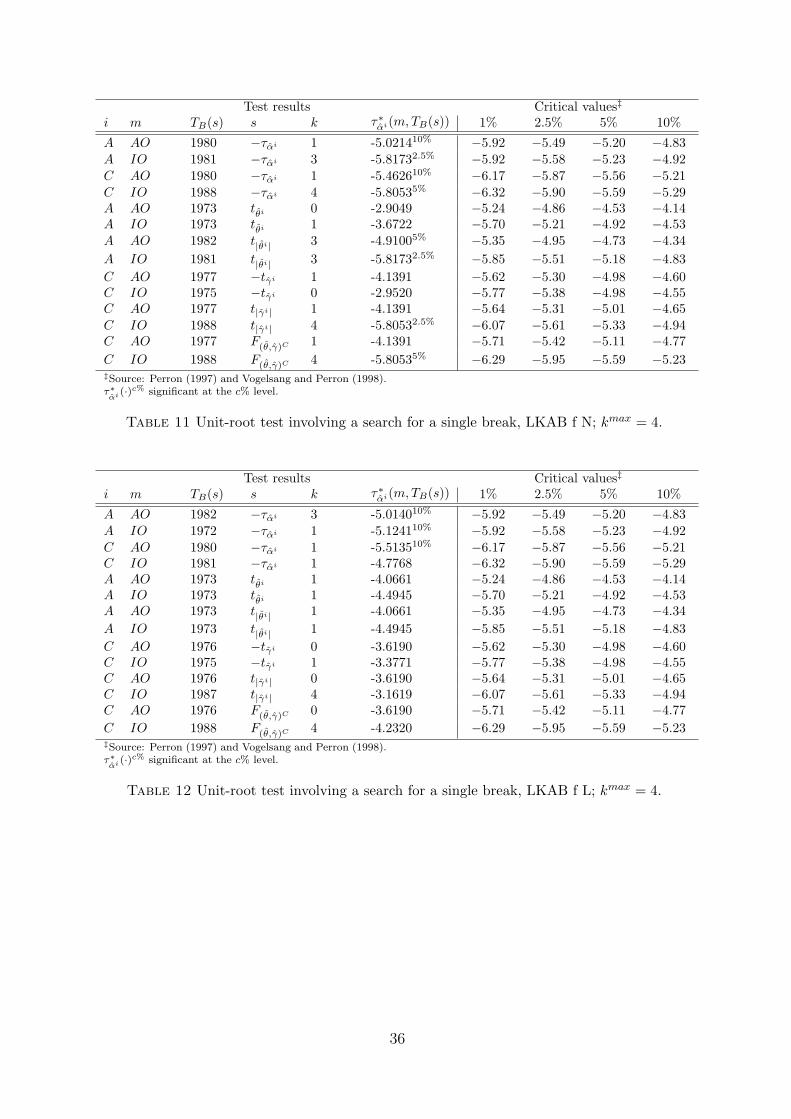
Test results Critical values‡

i m TB(s) s k τ∗αi(m,TB(s)) 1% 2.5% 5% 10%

A AO 1980 −ταi 1 -5.021410% −5.92 −5.49 −5.20 −4.83A IO 1981 −ταi 3 -5.81732.5% −5.92 −5.58 −5.23 −4.92C AO 1980 −ταi 1 -5.462610% −6.17 −5.87 −5.56 −5.21C IO 1988 −ταi 4 -5.80535% −6.32 −5.90 −5.59 −5.29A AO 1973 tθi 0 -2.9049 −5.24 −4.86 −4.53 −4.14A IO 1973 tθi 1 -3.6722 −5.70 −5.21 −4.92 −4.53A AO 1982 t|θi| 3 -4.91005% −5.35 −4.95 −4.73 −4.34A IO 1981 t|θi| 3 -5.81732.5% −5.85 −5.51 −5.18 −4.83C AO 1977 −tγi 1 -4.1391 −5.62 −5.30 −4.98 −4.60C IO 1975 −tγi 0 -2.9520 −5.77 −5.38 −4.98 −4.55C AO 1977 t|γi| 1 -4.1391 −5.64 −5.31 −5.01 −4.65C IO 1988 t|γi| 4 -5.80532.5% −6.07 −5.61 −5.33 −4.94C AO 1977 F(θ,γ)C 1 -4.1391 −5.71 −5.42 −5.11 −4.77C IO 1988 F(θ,γ)C 4 -5.80535% −6.29 −5.95 −5.59 −5.23‡Source: Perron (1997) and Vogelsang and Perron (1998).τ∗αi (·)c% significant at the c% level.

Table 11 Unit-root test involving a search for a single break, LKAB f N; kmax = 4.

Test results Critical values‡

i m TB(s) s k τ∗αi(m,TB(s)) 1% 2.5% 5% 10%

A AO 1982 −ταi 3 -5.014010% −5.92 −5.49 −5.20 −4.83A IO 1972 −ταi 1 -5.124110% −5.92 −5.58 −5.23 −4.92C AO 1980 −ταi 1 -5.513510% −6.17 −5.87 −5.56 −5.21C IO 1981 −ταi 1 -4.7768 −6.32 −5.90 −5.59 −5.29A AO 1973 tθi 1 -4.0661 −5.24 −4.86 −4.53 −4.14A IO 1973 tθi 1 -4.4945 −5.70 −5.21 −4.92 −4.53A AO 1973 t|θi| 1 -4.0661 −5.35 −4.95 −4.73 −4.34A IO 1973 t|θi| 1 -4.4945 −5.85 −5.51 −5.18 −4.83C AO 1976 −tγi 0 -3.6190 −5.62 −5.30 −4.98 −4.60C IO 1975 −tγi 1 -3.3771 −5.77 −5.38 −4.98 −4.55C AO 1976 t|γi| 0 -3.6190 −5.64 −5.31 −5.01 −4.65C IO 1987 t|γi| 4 -3.1619 −6.07 −5.61 −5.33 −4.94C AO 1976 F(θ,γ)C 0 -3.6190 −5.71 −5.42 −5.11 −4.77C IO 1988 F(θ,γ)C 4 -4.2320 −6.29 −5.95 −5.59 −5.23‡Source: Perron (1997) and Vogelsang and Perron (1998).τ∗αi (·)c% significant at the c% level.

Table 12 Unit-root test involving a search for a single break, LKAB f L; kmax = 4.

36

Test results Critical values‡

i m TB(s) s k τ∗αi(m,TB(s)) 1% 2.5% 5% 10%

A AO 1981 −ταi 3 -4.995210% −5.92 −5.49 −5.20 −4.83A IO 1981 −ταi 3 -5.57405% −5.92 −5.58 −5.23 −4.92C AO 1981 −ταi 3 -4.9965 −6.17 −5.87 −5.56 −5.21C IO 1987 −ταi 4 -5.74445% −6.32 −5.90 −5.59 −5.29A AO 1988 tθi 0 -2.7007 −5.24 −4.86 −4.53 −4.14A IO 1986 tθi 0 -2.5291 −5.70 −5.21 −4.92 −4.53A AO 1980 t|θi| 1 -4.718310% −5.35 −4.95 −4.73 −4.34A IO 1981 t|θi| 3 -5.57402.5% −5.85 −5.51 −5.18 −4.83C AO 1977 −tγi 3 -3.4449 −5.62 −5.30 −4.98 −4.60C IO 1975 −tγi 0 -2.7267 −5.77 −5.38 −4.98 −4.55C AO 1977 t|γi| 3 -3.4449 −5.64 −5.31 −5.01 −4.65C IO 1987 t|γi| 4 -5.74442.5% −6.07 −5.61 −5.33 −4.94C AO 1977 F(θ,γ)C 3 -3.4449 −5.71 −5.42 −5.11 −4.77C IO 1987 F(θ,γ)C 4 -5.74445% −6.29 −5.95 −5.59 −5.23‡Source: Perron (1997) and Vogelsang and Perron (1998).τ∗αi (·)c% significant at the c% level.

Table 13 Unit-root test involving a search for a single break, LKAB p; kmax = 4.

Test results Critical values‡

i m TB(s) s k τ∗αi(m,TB(s)) 1% 2.5% 5% 10%

A AO 1980 −ταi 1 -5.44225% −5.92 −5.49 −5.20 −4.83A IO 1981 −ταi 3 -5.39105% −5.92 −5.58 −5.23 −4.92C AO 1980 −ταi 1 -5.93712.5% −6.17 −5.87 −5.56 −5.21C IO 1982 −ταi 3 -4.7500 −6.32 −5.90 −5.59 −5.29A AO 1988 tθi 1 -2.8362 −5.24 −4.86 −4.53 −4.14A IO 1987 tθi 0 -2.2996 −5.70 −5.21 −4.92 −4.53A AO 1982 t|θi| 3 -4.0663 −5.35 −4.95 −4.73 −4.34A IO 1981 t|θi| 3 -5.39105% −5.85 −5.51 −5.18 −4.83C AO 1977 −tγi 2 -3.5232 −5.62 −5.30 −4.98 −4.60C IO 1976 −tγi 0 -3.1546 −5.77 −5.38 −4.98 −4.55C AO 1977 t|γi| 2 -3.5232 −5.64 −5.31 −5.01 −4.65C IO 1976 t|γi| 0 -3.1546 −6.07 −5.61 −5.33 −4.94C AO 1980 F(θ,γ)C 1 -5.9371 −5.71 −5.42 −5.11 −4.77C IO 1976 F(θ,γ)C 0 -3.1546 −6.29 −5.95 −5.59 −5.23‡Source: Perron (1997) and Vogelsang and Perron (1998).τ∗αi (·)c% significant at the c% level.

Table 14 Unit-root test involving a search for a single break, CVRD p; kmax = 4.

37

D Figures

1960 1970 1980 1990 2000

3.2

3.4

3.6The price of Brazilian fines

pt

1960 1970 1980 1990 2000

3.2

3.4

3.6OLS−fitted price from Model (A)

pt pt from Model (A)

1960 1970 1980 1990 2000

3.2

3.4

3.6OLS−fitted price from Model (B)

pt pt from Model (B)

1960 1970 1980 1990 2000

3.2

3.4

3.6OLS−fitted price from Model (C)

pt pt from Model (C)

Figure 3 pt under the alternative hypotheses of Models (A), (B), and (C), with AO;TB = 1973.

1970 1980 1990 2000

3.25

3.50

3.75

The price of LKAB fines f.o.b. Narvik

pt

1970 1980 1990 2000

3.25

3.50

3.75

OLS−fitted price from Model (A)

pt pt from Model (A)

1970 1980 1990 2000

3.25

3.50

3.75

OLS−fitted price from Model (B)

pt pt from Model (B)

1970 1980 1990 2000

3.25

3.50

3.75

OLS−fitted price from Model (C)

pt pt from Model (C)

Figure 4 pt under the alternative hypotheses of Models (A), (B), and (C), with AO;TB = 1973.

38

1970 1980 1990 2000

3.25

3.50

3.75

The price of LKAB fines f.o.b. Luleå

pt

1970 1980 1990 2000

3.25

3.50

3.75

OLS−fitted price from Model (A)

pt pt from Model (A)

1970 1980 1990 2000

3.25

3.50

3.75

OLS−fitted price from Model (B)

pt pt from Model (B)

1970 1980 1990 2000

3.25

3.50

3.75

OLS−fitted price from Model (C)

pt pt from Model (C)

Figure 5 pt under the alternative hypotheses of Models (A), (B), and (C), with AO;TB = 1973.

1970 1980 1990 2000

3.75

4.00

4.25

The price of LKAB pellets

pt

1970 1980 1990 2000

3.75

4.00

4.25

OLS−fitted price from Model (A)

pt pt from Model (A)

1970 1980 1990 2000

3.75

4.00

4.25

OLS−fitted price from Model (B)

pt pt from Model (B)

1970 1980 1990 2000

3.75

4.00

4.25

OLS−fitted price from Model (C)

pt pt from Model (C)

Figure 6 pt under the alternative hypotheses of Models (A), (B), and (C), with AO;TB = 1973.

39

1970 1980 1990 2000

3.75

4.00

4.25The price of CVRD pellets f.o.b. Tubarão

pt

1970 1980 1990 2000

3.50

3.75

4.00

4.25OLS−fitted price from Model (A)

pt pt from Model (A)

1970 1980 1990 2000

3.75

4.00

4.25OLS−fitted price from Model (B)

pt pt from Model (B)

1970 1980 1990 2000

3.50

3.75

4.00

4.25OLS−fitted price from Model (C)

pt pt from Model (C)

Figure 7 pt under the alternative hypotheses of Models (A), (B), and (C), with AO;TB = 1973.

40

WORKING PAPERS* Editor: Nils Gottfries 2005:6 Katarina Nordblom and Henry Ohlsson, Tax Avoidance and Intra-Family

Transfers. 25 pp. 2005:7 Sören Blomquist and Luca Micheletto, Optimal Redistributive Taxation

when Government’s and Agents’ Preferences Differ. 22 pp. 2005:8 Ruth-Aïda Nahum, Income Inequality and Growth: A Panel Study of

Swedish Counties 1960-2000. 39 pp. 2005:9 Olof Åslund and Peter Fredriksson, Ethnic Enclaves and Welfare Cultures –

Quasi-experimental Evidence. 37 pp. 2005:10 Annika Alexius and Erik Post, Exchange Rates and Asymmetric Shocks in

Small Open Economies. 31 pp. 2005:11 Martin Ågren, Myopic Loss Aversion, the Equity Premium Puzzle, and

GARCH. 34 pp. 2005:12 Pär Holmberg, Numerical Calculation of an Asymmetric Supply Function

Equilibrium with Capacity Constraints. 18 pp. 2005:13 Jovan Zamac, Winners and Losers from a Demographic Shock under

Different Intergenerational Transfer Schemes. 44 pp. 2005:14 Peter Welz and Pär Österholm, Interest Rate Smoothing versus Serially

Correlated Errors in Taylor Rules: Testing the Tests. 29 pp. 2005:15 Helge Bennmarker, Kenneth Carling and Bertil Holmlund, Do Benefit

Hikes Damage Job Finding? Evidence from Swedish Unemployment Insurance Reforms. 37 pp.

2005:16 Pär Holmberg, Asymmetric Supply Function Equilibrium with Constant

Marginal Costs. 27 pp. 2005:17 Pär Holmberg: Comparing Supply Function Equilibria of Pay-as-Bid and

Uniform-Price Auctions. 25 pp. 2005:18 Anders Forslund, Nils Gottfries and Andreas Westermark: Real and

Nominal Wage Adjustment in Open Economies. 49 pp. 2005:19 Lennart Berg and Tommy Berger, The Q Theory and the Swedish Housing

Market – An Empirical Test. 16 pp. 2005:20 Matz Dahlberg and Magnus Gustavsson, Inequality and Crime: Separating

the Effects of Permanent and Transitory Income. 27 pp. * A list of papers in this series from earlier years will be sent on request by the department.

2005:21 Jenny Nykvist, Entrepreneurship and Liquidity Constraints: Evidence from Sweden. 29 pp.

2005:22 Per Engström och Bertil Holmlund, Jenny Nykvist: Worker Absenteeism in

Search Equilibrium. 35pp. 2005:23 Peter Hästö och Pär Holmberg, Some inequalities related to the analysis of

electricity auctions. 7pp. 2006:1 Jie Chen, The Dynamics of Housing Allowance Claims in Sweden: A

discrete-time hazard analysis. 37pp. 2006:2 Fredrik Johansson and Anders Klevmarken: Explaining the size and

nature of response in a survey on health status and economic standard. 25pp.

2006:3 Magnus Gustavsson and Henrik Jordahl, Inequality and Trust: Some Inequalities are More Harmful than Others. 29pp.

2006:4 N. Anders Klevmarken, The Distribution of Wealth in Sweden: Trends and

Driving factors. 20pp. 2006:5 Erica Lindahl and Andreas Westermark: Soft Budget Constraints as a Risk

Sharing Arrangement in an Economic Federation. 22pp. 2006:6 Jonas Björnerstedt and Andreas Westermark: Bargaining and Strategic

Discrimination. 36pp. 2006:7 Mikael Carlsson, Stefan Eriksson and Nils Gottfries: Testing Theories of Job

Creation: Does Supply Create Its Own Demand? 23pp. 2006:8 Annika Alexius and Erik Post, Cointegration and the stabilizing role of

exchange rates. 33pp. 2006:9 David Kjellberg, Measuring Expectations. 46pp. 2006:10 Nikolay Angelov, Modellig firm mergers as a roommate problem. 21pp. 2006:11 Nikolay Angelov, Structural breaks in iron-ore prices: The impact of the

1973 oil crisis. 41pp. See also working papers published by the Office of Labour Market Policy Evaluation http://www.ifau.se/ ISSN 1653-6975