Transitions Between Hover and Level Flight for a Tailsitter...
98
TRANSITIONS BETWEEN HOVER AND LEVEL FLIGHT FOR A TAILSITTER UAV by Stephen R. Osborne A thesis submitted to the faculty of Brigham Young University in partial fulfillment of the requirements for the degree of Master of Science Department of Electrical and Computer Engineering Brigham Young University December 2007
-
Upload
nguyenduong -
Category
Documents
-
view
215 -
download
0
Transcript of Transitions Between Hover and Level Flight for a Tailsitter...
TRANSITIONS BETWEEN HOVER AND LEVEL FLIGHT FOR A
TAILSITTER UAV
by
Stephen R. Osborne
A thesis submitted to the faculty of
Brigham Young University
in partial fulfillment of the requirements for the degree of
Master of Science
Department of Electrical and Computer Engineering
Brigham Young University
December 2007

Copyright c© 2007 Stephen R. Osborne
All Rights Reserved

BRIGHAM YOUNG UNIVERSITY
GRADUATE COMMITTEE APPROVAL
of a thesis submitted by
Stephen R. Osborne
This thesis has been read by each member of the following graduate committee andby majority vote has been found to be satisfactory.
Date Randal W. Beard, Chair
Date Timothy W. McLain
Date D.J. Lee

BRIGHAM YOUNG UNIVERSITY
As chair of the candidate’s graduate committee, I have read the thesis of StephenR. Osborne in its final form and have found that (1) its format, citations, and bibli-ographical style are consistent and acceptable and fulfill university and departmentstyle requirements; (2) its illustrative materials including figures, tables, and chartsare in place; and (3) the final manuscript is satisfactory to the graduate committeeand is ready for submission to the university library.
Date Randal W. BeardChair, Graduate Committee
Accepted for the Department
Michael A. JensenChair
Accepted for the College
Alan R. ParkinsonDean, Ira A. Fulton College ofEngineering and Technology


ABSTRACT
TRANSITIONS BETWEEN HOVER AND LEVEL FLIGHT FOR A
TAILSITTER UAV
Stephen R. Osborne
Department of Electrical and Computer Engineering
Master of Science
Vertical Take-Off and Land (VTOL) Unmanned Air Vehicles (UAVs) possess
several desirable characteristics, such as being able to hover and take-off or land in
confined areas. One type of VTOL airframe, the tailsitter, has all of these advan-
tages, as well as being able to fly in the more energy-efficient level flight mode. The
tailsitter can track trajectories that successfully transition between hover and level
flight modes. Three methods for performing transitions are described: a simple con-
troller, a feedback linearization controller, and an adaptive controller. An autopilot
navigational state machine with appropriate transitioning between level and hover
waypoints is also presented. The simple controller is useful for performing a immedi-
ate transition. It is very quick to react and maintains altitude during the maneuver,
but tracking is not performed in the lateral direction. The feedback linearization
controller and adaptive controller both perform equally well at tracking transition
trajectories in lateral and longitudinal directions, but the adaptive controller requires
knowledge of far fewer parameters.

ACKNOWLEDGEMENTS
I would first like to thank the members of my committee for their support and
guidance in the creation of this thesis. Dr. Beard and Dr. McLain also deserve my
gratitude for their leadership in the Magicc Lab, where I have worked for the past two
years. Dr. Beard has also been an invaluable resource in directing my research and
proofreading this thesis numerous times. Along with these professors, I also thank all
my fellow Magicc Labbers who have helped me in any way, shape, or form during my
stay here. Special thanks goes to Nate Knoebel for his assistance and expertise on
tailsitter issues, as well as for many hours spent during flight testing in the summer
heat.

Table of Contents
Acknowledgements xi
List of Tables xvii
List of Figures xix
1 Introduction 1
1.1 Background and Motivation . . . . . . . . . . . . . . . . . . . . . . . 1
1.2 Literature Review . . . . . . . . . . . . . . . . . . . . . . . . . . . . . 3
1.3 Contributions . . . . . . . . . . . . . . . . . . . . . . . . . . . . . . . 5
1.4 Document Organization . . . . . . . . . . . . . . . . . . . . . . . . . 5
2 Tailsitter Physics 7
2.1 Three-dimensional Model . . . . . . . . . . . . . . . . . . . . . . . . . 7
2.1.1 Quaternion Motivation and Definition . . . . . . . . . . . . . . 7
2.1.2 Quaternion/Euler Conversions . . . . . . . . . . . . . . . . . . 9
2.1.3 Navigation Equations . . . . . . . . . . . . . . . . . . . . . . . 9
2.1.4 Kinematic Equations . . . . . . . . . . . . . . . . . . . . . . . 10
2.1.5 Force Equations . . . . . . . . . . . . . . . . . . . . . . . . . . 11
2.2 Two-dimensional Model . . . . . . . . . . . . . . . . . . . . . . . . . 13
2.3 Chapter Summary . . . . . . . . . . . . . . . . . . . . . . . . . . . . 17
3 Experimental Platform 19
xiii
3.1 Simulation . . . . . . . . . . . . . . . . . . . . . . . . . . . . . . . . . 19
3.2 Flight Test Setup . . . . . . . . . . . . . . . . . . . . . . . . . . . . . 19
3.3 Quaternion Attitude Control . . . . . . . . . . . . . . . . . . . . . . . 21
3.4 Hover Position Control . . . . . . . . . . . . . . . . . . . . . . . . . . 23
3.5 Level Flight Control . . . . . . . . . . . . . . . . . . . . . . . . . . . 26
3.6 Chapter Summary . . . . . . . . . . . . . . . . . . . . . . . . . . . . 28
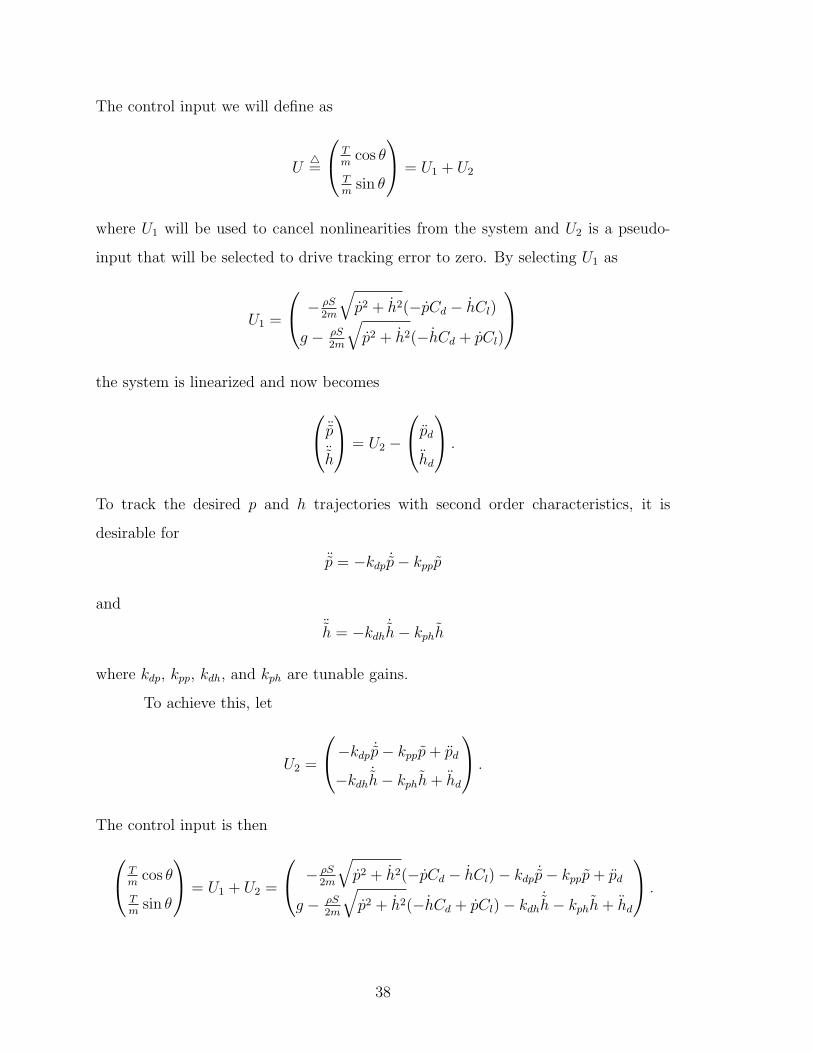
4 Trajectory Tracking Algorithms 31
4.1 Desired Trajectories . . . . . . . . . . . . . . . . . . . . . . . . . . . . 31
4.2 Simple Controller . . . . . . . . . . . . . . . . . . . . . . . . . . . . . 35
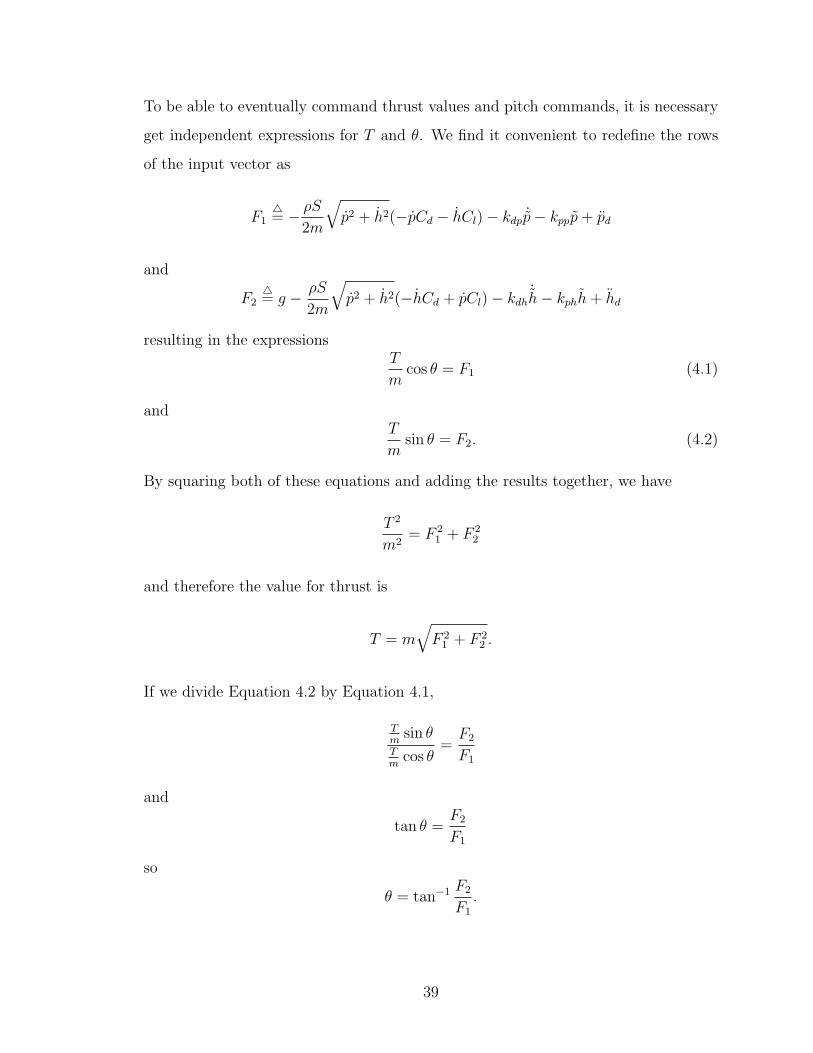
4.3 Feedback Linearization Controller . . . . . . . . . . . . . . . . . . . . 37
4.4 Adaptive Controller . . . . . . . . . . . . . . . . . . . . . . . . . . . . 40
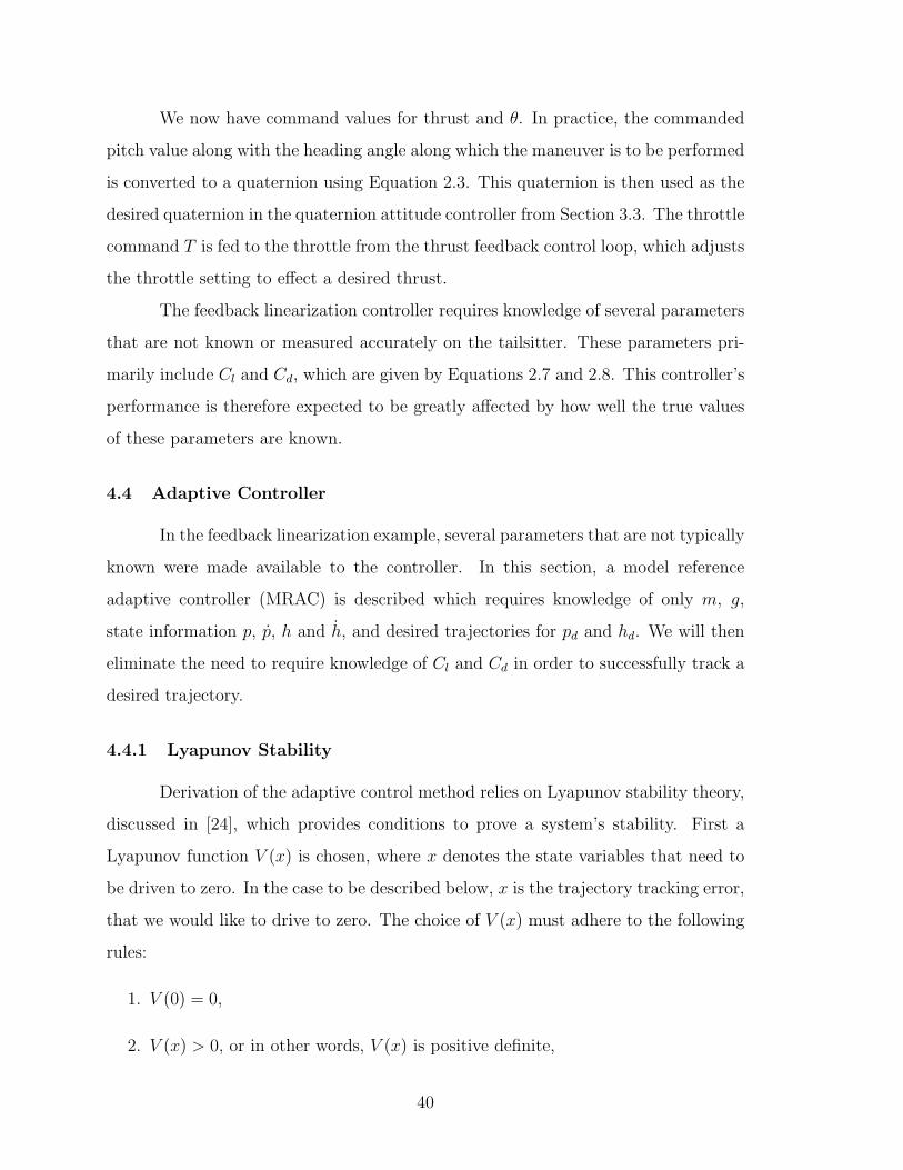
4.4.1 Lyapunov Stability . . . . . . . . . . . . . . . . . . . . . . . . 40
4.4.2 Equations of Motion . . . . . . . . . . . . . . . . . . . . . . . 41
4.4.3 Reference Model . . . . . . . . . . . . . . . . . . . . . . . . . 41
4.4.4 Controller Derivation . . . . . . . . . . . . . . . . . . . . . . . 42
4.5 Simulation Results . . . . . . . . . . . . . . . . . . . . . . . . . . . . 45
4.5.1 Simple Controller Simulations . . . . . . . . . . . . . . . . . . 46
4.5.2 Feedback Linearization Controller Simulations . . . . . . . . . 48
4.5.3 Adaptive Controller Simulations . . . . . . . . . . . . . . . . . 50
4.6 Flight Test Results . . . . . . . . . . . . . . . . . . . . . . . . . . . . 53
4.6.1 Simple Controller Flight Results . . . . . . . . . . . . . . . . . 53
4.6.2 Feedback Linearization Controller Flight Results . . . . . . . . 56
4.6.3 Adaptive Controller Flight Results . . . . . . . . . . . . . . . 59
4.7 Chapter Summary . . . . . . . . . . . . . . . . . . . . . . . . . . . . 62
5 Autopilot State Machine 63
xiv
5.1 Autopilot Structure . . . . . . . . . . . . . . . . . . . . . . . . . . . . 63
5.2 Autopilot Flight Results with Simple Controller . . . . . . . . . . . . 66
5.3 Autopilot Flight Results with Feedback Linearization Controller . . . 69
5.4 Autopilot Flight Results with Adaptive Controller . . . . . . . . . . . 71
5.5 Chapter Summary . . . . . . . . . . . . . . . . . . . . . . . . . . . . 73
6 Conclusion 75
6.1 Summary of Results . . . . . . . . . . . . . . . . . . . . . . . . . . . 75
6.2 Future Work . . . . . . . . . . . . . . . . . . . . . . . . . . . . . . . . 75
Bibliography 77
xv

xvi
List of Tables
5.1 Autopilot state machine state numbers . . . . . . . . . . . . . . . . . 67
xvii

xviii
List of Figures
1.1 Convair XFY-1 Pogo, 1954 . . . . . . . . . . . . . . . . . . . . . . . . 2
1.2 Ryan X-13 Vertijet, 1956 . . . . . . . . . . . . . . . . . . . . . . . . . 2
2.1 Lift and drag coefficients versus α. . . . . . . . . . . . . . . . . . . . 13
2.2 Forces acting on tailsitter . . . . . . . . . . . . . . . . . . . . . . . . 14
3.1 The Magicc Lab Pogo airframe . . . . . . . . . . . . . . . . . . . . . 20
3.2 Kestrel Autopilot . . . . . . . . . . . . . . . . . . . . . . . . . . . . . 21
3.3 Quaternion attitude controller performance in flight test . . . . . . . 24
3.4 Hover position tracking flight data . . . . . . . . . . . . . . . . . . . . 27
3.5 Level waypoint tracking flight data . . . . . . . . . . . . . . . . . . . 29
4.1 Hover-to-level trajectory goal . . . . . . . . . . . . . . . . . . . . . . 32
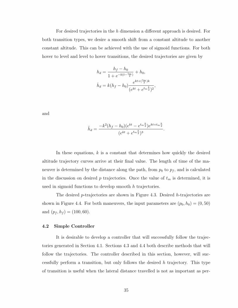
4.2 Level-to-hover trajectory goal . . . . . . . . . . . . . . . . . . . . . . 32
4.3 Desired p-trajectories . . . . . . . . . . . . . . . . . . . . . . . . . . . 34
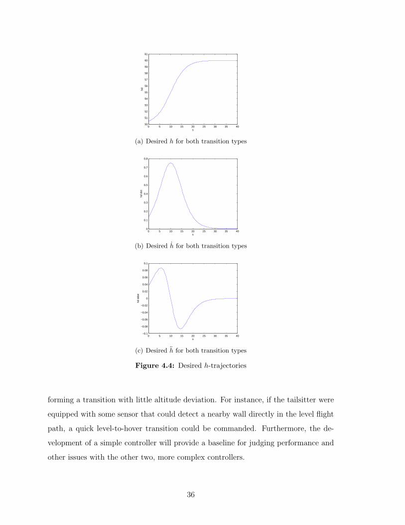
4.4 Desired h-trajectories . . . . . . . . . . . . . . . . . . . . . . . . . . . 36
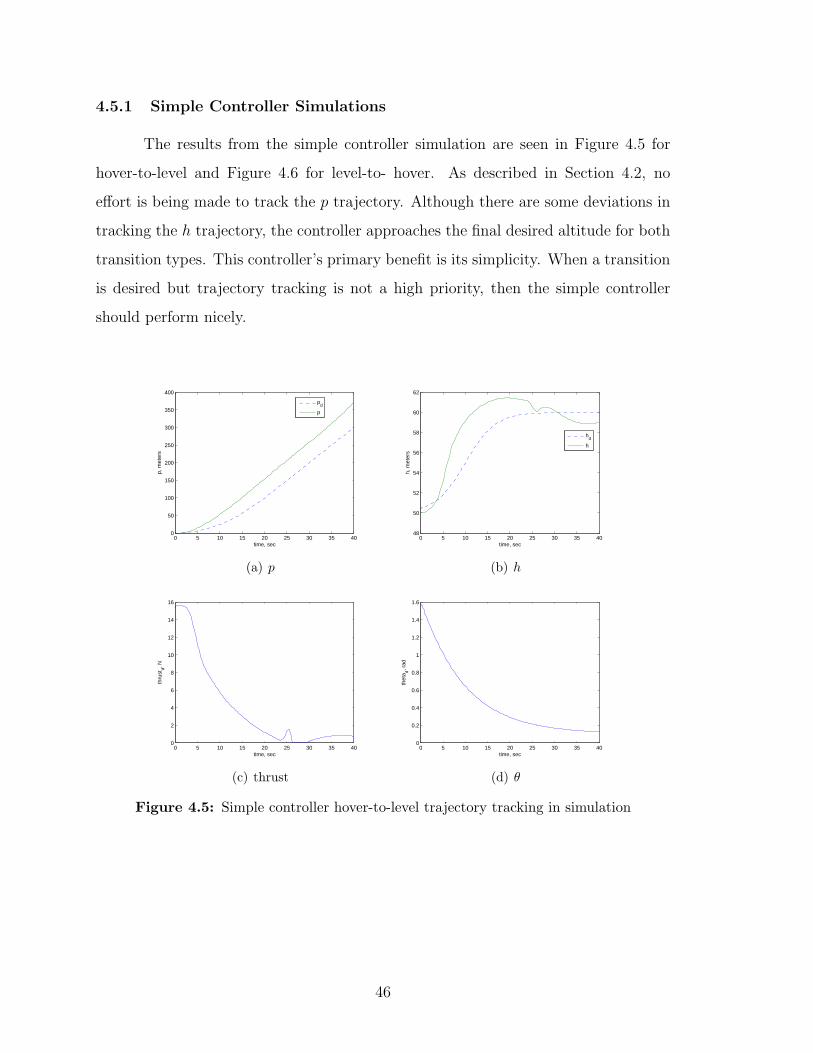
4.5 Simple controller hover-to-level trajectory tracking in simulation . . . 46
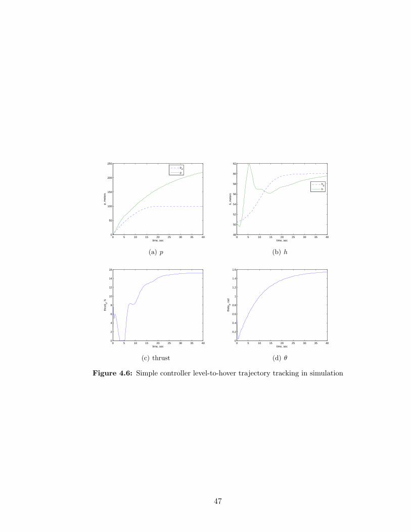
4.6 Simple controller level-to-hover trajectory tracking in simulation . . . 47
4.7 Feedback linearization controller hover-to-level trajectory tracking insimulation . . . . . . . . . . . . . . . . . . . . . . . . . . . . . . . . . 48
4.8 Feedback linearization controller level-to-hover trajectory tracking insimulation . . . . . . . . . . . . . . . . . . . . . . . . . . . . . . . . . 49
4.9 Adaptive controller hover-to-level trajectory tracking in simulation . . 51
xix
4.10 Adaptive controller level-to-hover trajectory tracking in simulation . . 52
4.11 Simple controller hover-to-level transition flight data . . . . . . . . . 54
4.12 Simple controller level-to-hover transition flight data . . . . . . . . . 55
4.13 Feedback linearization controller hover-to-level trajectory tracking flightdata . . . . . . . . . . . . . . . . . . . . . . . . . . . . . . . . . . . . 57
4.14 Feedback linearization controller level-to-hover trajectory tracking flightdata . . . . . . . . . . . . . . . . . . . . . . . . . . . . . . . . . . . . 58
4.15 Adaptive controller hover-to-level trajectory tracking flight data . . . 60
4.16 Adaptive controller level-to-hover trajectory tracking flight data . . . 61
5.1 Autopilot state machine . . . . . . . . . . . . . . . . . . . . . . . . . 64
5.2 State machine flight results with simple controller . . . . . . . . . . . 68
5.3 State machine flight results with feedback linearization controller . . . 70
5.4 State machine flight results with adaptive controller . . . . . . . . . . 72
xx
Chapter 1
Introduction
1.1 Background and Motivation
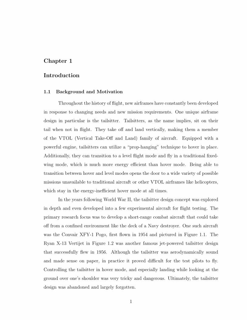
Throughout the history of flight, new airframes have constantly been developed
in response to changing needs and new mission requirements. One unique airframe
design in particular is the tailsitter. Tailsitters, as the name implies, sit on their
tail when not in flight. They take off and land vertically, making them a member
of the VTOL (Vertical Take-Off and Land) family of aircraft. Equipped with a
powerful engine, tailsitters can utilize a “prop-hanging” technique to hover in place.
Additionally, they can transition to a level flight mode and fly in a traditional fixed-
wing mode, which is much more energy efficient than hover mode. Being able to
transition between hover and level modes opens the door to a wide variety of possible
missions unavailable to traditional aircraft or other VTOL airframes like helicopters,
which stay in the energy-inefficient hover mode at all times.
In the years following World War II, the tailsitter design concept was explored
in depth and even developed into a few experimental aircraft for flight testing. The
primary research focus was to develop a short-range combat aircraft that could take
off from a confined environment like the deck of a Navy destroyer. One such aircraft
was the Convair XFY-1 Pogo, first flown in 1954 and pictured in Figure 1.1. The
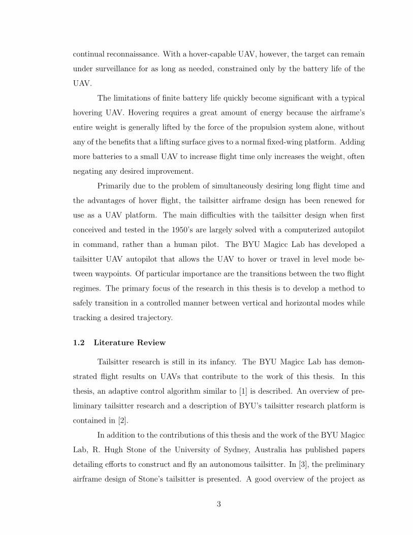
Ryan X-13 Vertijet in Figure 1.2 was another famous jet-powered tailsitter design
that successfully flew in 1956. Although the tailsitter was aerodynamically sound
and made sense on paper, in practice it proved difficult for the test pilots to fly.
Controlling the tailsitter in hover mode, and especially landing while looking at the
ground over one’s shoulder was very tricky and dangerous. Ultimately, the tailsitter
design was abandoned and largely forgotten.
1
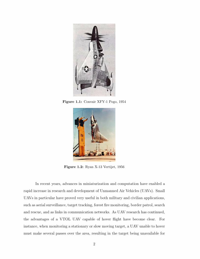
Figure 1.1: Convair XFY-1 Pogo, 1954
Figure 1.2: Ryan X-13 Vertijet, 1956
In recent years, advances in miniaturization and computation have enabled a
rapid increase in research and development of Unmanned Air Vehicles (UAVs). Small
UAVs in particular have proved very useful in both military and civilian applications,
such as aerial surveillance, target tracking, forest fire monitoring, border patrol, search
and rescue, and as links in communication networks. As UAV research has continued,
the advantages of a VTOL UAV capable of hover flight have become clear. For
instance, when monitoring a stationary or slow moving target, a UAV unable to hover
must make several passes over the area, resulting in the target being unavailable for
2
continual reconnaissance. With a hover-capable UAV, however, the target can remain
under surveillance for as long as needed, constrained only by the battery life of the
UAV.
The limitations of finite battery life quickly become significant with a typical
hovering UAV. Hovering requires a great amount of energy because the airframe’s
entire weight is generally lifted by the force of the propulsion system alone, without
any of the benefits that a lifting surface gives to a normal fixed-wing platform. Adding
more batteries to a small UAV to increase flight time only increases the weight, often
negating any desired improvement.
Primarily due to the problem of simultaneously desiring long flight time and
the advantages of hover flight, the tailsitter airframe design has been renewed for
use as a UAV platform. The main difficulties with the tailsitter design when first
conceived and tested in the 1950’s are largely solved with a computerized autopilot
in command, rather than a human pilot. The BYU Magicc Lab has developed a
tailsitter UAV autopilot that allows the UAV to hover or travel in level mode be-
tween waypoints. Of particular importance are the transitions between the two flight
regimes. The primary focus of the research in this thesis is to develop a method to
safely transition in a controlled manner between vertical and horizontal modes while
tracking a desired trajectory.
1.2 Literature Review
Tailsitter research is still in its infancy. The BYU Magicc Lab has demon-
strated flight results on UAVs that contribute to the work of this thesis. In this
thesis, an adaptive control algorithm similar to [1] is described. An overview of pre-
liminary tailsitter research and a description of BYU’s tailsitter research platform is
contained in [2].
In addition to the contributions of this thesis and the work of the BYU Magicc
Lab, R. Hugh Stone of the University of Sydney, Australia has published papers
detailing efforts to construct and fly an autonomous tailsitter. In [3], the preliminary
airframe design of Stone’s tailsitter is presented. A good overview of the project as
3
well as a description of possible applications for tailsitters is given in [4]. The control
and guidance architecture is presented in [5]. Of particular interest to this thesis is
[6], which describes optimization methods of the tailsitter’s stall-tumble maneuver
transitions between hover and level flight.
Although not much literature is available detailing their efforts, a tailsitter
UAV named SkyTote has been under development since 1998 by AeroVironment
[7], a company specializing in unmanned aircraft systems. As discussed in [8], the
SkyTote is being designed as a precision cargo delivery system, capable of delivering
a 50 pound payload to within a 15 foot area up to 200 miles away from the mission
start point, with a 1.5 hour max battery life. Mission parameters like these are ideal
for a tailsitter which has the precision landing capability of a hovering UAV and the
energy-efficiency of a fixed wing airframe. At this time, it is unknown what progress
has been made on the SkyTote system.
Green and Oh at Drexel University have contributed several papers of interest
to tailsitter research. Although the flight platform described is not a tailsitter, it can
transition between level and hover flight. Much of the research focus is on developing
a UAV that can fly in confined spaces, such as inside buildings. These efforts are de-
scribed in [9], [10] and [11]. The same authors also use vision-based guidance systems
to control small MAVs with similar hover characteristics to a miniature tailsitter in
[12], [13], and [14].
Other authors contribute useful theoretical discussion applicable to tailsitter
research. Methods for trajectory tracking with a VTOL aircraft are presented in
[15], [16], and [17]. Costic, et. al., [18] describe a quaternion-based attitude track-
ing controller for spacecraft. Trajectory tracking for fixed-wing UAVs performing
aggressive flight maneuvers is explored in [19]. An excellent description of attitude
representations, including an extensive description of the quaternion representation,
is presented in [20].
4
1.3 Contributions
The research described in this thesis presents three different control methods
which may be used for transitioning a VTOL tailsitter UAV between hover and level
flight modes. Simulation and flight test results for each of the modes are also pre-
sented. The tailsitter physics models used in the derivation as well as simulation of
the control methods are also given, and will prove useful to others seeking to further
develop tailsitter autopilot technology. Finally, a tailsitter navigational autopilot is
presented which provides a framework for flying a flight plan composed of hover and
level waypoints.
1.4 Document Organization
In Chapter 2, both 2D and 3D physics models are presented that will be
used in later derivations of controllers as well as for testing the algorithms in simu-
lation. Chapter 3 describes the simulation and hardware environments used in this
research. Chapter 4 contains derivations for simple, feedback linearization, and adap-
tive controllers for negotiating transitions between flight modes for a tailsitter UAV.
Simulation and flight test results for transitions are also included. In Chapter 5, a
navigational autopilot for flying a flight path composed of mixed hover and level way-
points is described and flight results are given. Conclusions and recommendations for
future work are given in Chapter 6.
5

6
Chapter 2
Tailsitter Physics
The starting point for developing trajectory tracking control is to develop an
accurate physical model of the system. Two models are presented in this chapter,
describing three-dimensional and two-dimensional dynamics. The three-dimensional,
quaternion-based, high fidelity model is used in simulation testing of the tracking
algorithms, but is too complex to be used as the basis for developing implementable
control. Therefore, a two-dimensional model that captures the essential features of
the system is used to develop the control algorithms.
2.1 Three-dimensional Model
The three-dimensional physics model uses a quaternion representation of tail-
sitter attitude. Quaternions, as described in this section, provide a unique description
of attitude without the singularity introduced in a hover position by an Euler angle
attitude representation.
2.1.1 Quaternion Motivation and Definition
Euler angles are traditionally used to represent aircraft attitude in aerospace
literature. Starting from an aircraft orientation with the nose facing North (the
world frame x axis), the right wing facing East (the world frame y axis) and the
belly facing down (the world frame z axis), each angle signifies a rotation about an
individual axis. The order of rotations is non-commutative and so a standard order
of rotations is used. First the aircraft is rotated about the z axis by ψ, called the
yaw angle. Then the aircraft is rotated about the newly created y axis by θ, the pitch
angle. The final rotation is about the new x axis and is called the roll angle, φ.
7
Euler angles are an intuitive measure of the aircraft’s attitude and thus are very
useful in aircraft control. However, this Euler angle representation has singularities
at θ = ±π2. At these points when the pitch angle is pointed straight up or straight
down, a situation called gimbal lock occurs where the body-fixed x and inertial z axes
are now aligned. This situation is analogous to being at the North or South pole of
the Earth where all longitudinal lines come together at a point, or singularity. At
the North pole, for instance, all directions point south. For the aircraft Euler angle
representation, no yaw information can be gathered at the singularities and attitude
cannot be properly determined. Quaternions, fortunately, do not suffer from gimbal
lock and provide a singularity-free version of attitude representation.
A quaternion contains four elements and may be thought of as the composition
of an axis of rotation and an angle specifying the magnitude of rotation about that
axis. A rotation of Θ radians about a three-dimensional vector ~v is represented as
the quaternion
η =
η1
η2
η3
η4
=
sin Θ2v1
sin Θ2v2
sin Θ2v3
cos Θ2
. (2.1)
For the tailsitter, attitude can be described with a single quaternion. This attitude
quaternion represents the axis of rotation (defined in the world frame) and magnitude
of rotation to achieve the current tailsitter orientation when starting from the initial
attitude of nose facing North and right wing facing East.
8
2.1.2 Quaternion/Euler Conversions
A unit quaternion can be translated to traditional Euler angle representation
by the transformation
φ
θ
ψ
=
tan−1 2(η2η3+η4η1)
1−2(η21+η2
2)
sin−1(−2(η1η3 − η4η2))
tan−1 2(η1η2+η4η3)
1−2(η22+η2
3)
(2.2)
and Euler angles are converted to a quaternion by
η1
η2
η3
η4
=
sin φ2
cos θ2cos ψ
2− cos φ
2sin θ
2sin ψ
2
cos φ2
sin θ2cos ψ
2+ sin φ
2cos θ
2sin ψ
2
cos φ2
cos θ2sin ψ
2− sin φ
2sin θ
2cos ψ
2
cos φ2
cos θ2cos ψ
2+ sin φ
2sin θ
2sin ψ
2
. (2.3)
Due to the singularity at θ = ±π2, care must be taken when converting from a quater-
nion to Euler angles when the pitch of the aircraft is near these values, as ψ will be
indeterminate.
2.1.3 Navigation Equations
Body frame velocities are translated to the inertial frame by
x
y
z
=
cos θ cos ψ sin φ sin θ cos ψ − cos φ sin ψ cos φ sin θ cos ψ + sin φ sin ψ
cos θ sin ψ sin φ sin θ sin ψ + cos φ cos ψ cos φ sin θ sin ψ − sin φ cos ψ
− sin θ sin φ cos θ cos φ cos θ
u
v
w
or, with quaternions,
x
y
z
=
1− 2(η22 + η2
3) 2(η1η2 − η4η3) 2(η1η3 + η4η2)
2(η1η2 + η4η3) 1− 2(η21 + η2
3) 2(η2η3 − η4η1)
2(η1η3 − η4η2) 2(η2η3 + η4η1) 1− 2(η21 + η2
2)
u
v
w
. (2.4)
9
2.1.4 Kinematic Equations
We assume a quaternion-based attitude controller. The quaternion update
equation is
η =1
2AΩ
with
A =
η4 −η3 η2
η3 η4 −η1
−η2 η1 η4
−η1 −η2 −η3
and
Ω =
p
q
r
where p, q, and r are angular velocities about the body frame x, y, and z axes,
respectively. The angular rates are updated by
Ω = kΩ(Ωc − Ω)
where
Ωc = keηe − kdΩ.
In these equations, kΩ, ke, and kd are gains and ηe is known as the error quaternion,
given by
10
ηe =
η4 η3 −η2 −η1
−η3 η4 η1 −η2
η2 −η1 η4 −η3
η1 η2 η3 η4
ηc.
The error quaternion is the error between the tailsitter’s current attitude, given by
η, and the desired attitude, ηc. The attitude controller adjusts the angular rates p, q,
and r to achieve the desired orientation. In practice, the angular rates are adjusted
by controlling the aileron, elevator, and rudder control surfaces.
2.1.5 Force Equations
World frame accelerations are found by taking the derivative of (2.4):
x
y
z
= N
u
v
w
+ N
u
v
w
(2.5)
= NV + NV (2.6)
where N is the rotation matrix from (2.4) and
N =
−4η3η3 − 4η4η4 2η2η3 + 2η2η3 − 2η1η4 − 2η1η4
2η2η3 + 2η2η3 + 2η1η4 + 2η1η4 −4η2η2 − 4η4η4
2η2η4 + 2η2η4 − 2η1η3 − 2η1η3 2η3η4 + 2η3η4 + 2η1η2 + 2η1η2
2η2η4 + 2η2η4 + 2η1η3 + 2η1η3
2η3η4 + 2η3η4 − 2η1η2 − 2η1η2
−4η2η2 − 4η3η3
and
V = (−Ω× V ) + N−1G +1
mT +
1
mL +
1
mD
11
where G is the world frame gravity vector, T is the thrust vector, and L and D are
lift and drag vectors given by
L =ρV 2S
2
sin αCl(α)
0
− cos αCl(α)
and
D =ρV 2S
2
− cos αCd(α)
0
− sin αCd(α)
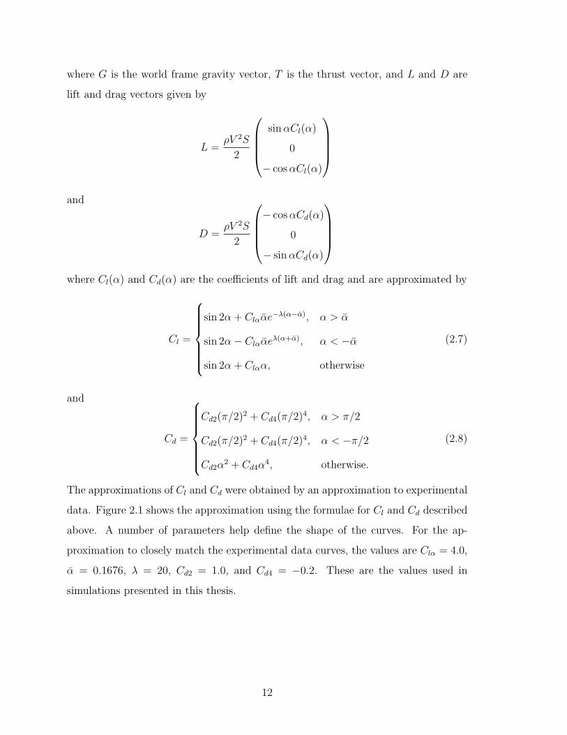
where Cl(α) and Cd(α) are the coefficients of lift and drag and are approximated by
Cl =
sin 2α + Clααe−λ(α−α), α > α
sin 2α− Clααeλ(α+α), α < −α
sin 2α + Clαα, otherwise
(2.7)
and
Cd =
Cd2(π/2)2 + Cd4(π/2)4, α > π/2
Cd2(π/2)2 + Cd4(π/2)4, α < −π/2
Cd2α2 + Cd4α
4, otherwise.
(2.8)
The approximations of Cl and Cd were obtained by an approximation to experimental
data. Figure 2.1 shows the approximation using the formulae for Cl and Cd described
above. A number of parameters help define the shape of the curves. For the ap-
proximation to closely match the experimental data curves, the values are Clα = 4.0,
α = 0.1676, λ = 20, Cd2 = 1.0, and Cd4 = −0.2. These are the values used in
simulations presented in this thesis.
12
−100 −50 0 50 100−1.5
−1
−0.5
0
0.5
1
1.5
α (degrees)
CL
−100 −50 0 50 1000
0.5
1
1.5
α (degrees)
CD
Figure 2.1: Lift and drag coefficients versus α.
After substituting in the kinematic equation for η, as well as enforcing the
quaternion unit norm constraint, the force equations simplify to
x
y
z
=
( Tm
+ Ax
m)(1− 2η2
3 − 2η24) + Az
m(2η1η3 + 2η2η4)
( Tm
+ Ax
m)(2η1η4 + 2η2η3) + Az
m(2η3η4 − 2η1η2)
( Tm
+ Ax
m)(2η2η4 − 2η1η3) + Az
m(1− 2η2
2 − 2η23) + g
(2.9)
where Ax and Az are the combined aerodynamic lift and drag forces given by
Ax =ρV 2S
2(sin αCl(α)− cos αCd(α))
and
Az =ρV 2S
2(− cos αCl(α)− sin αCd(α)).
2.2 Two-dimensional Model
In the course of this research, the three-dimensional tailsitter physics model
proved difficult to work with in the development of a transition controller. Resulting
controllers were overly complex due to the large number of control inputs (T , η1,
η2, η3, and η4) and the nature of these inputs being interspersed throughout the
13
force equations. For the scope and purpose of this thesis, it is convenient to derive a
simpler, two-dimensional physics model and develop controllers based upon it. Since
the transitions will be performed in the direction of current heading of the tailsitter,
the extra dimension is not necessary in any case.
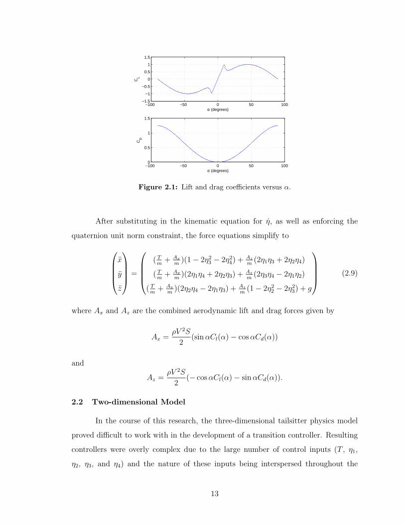
Figure 2.2: Forces acting on tailsitter
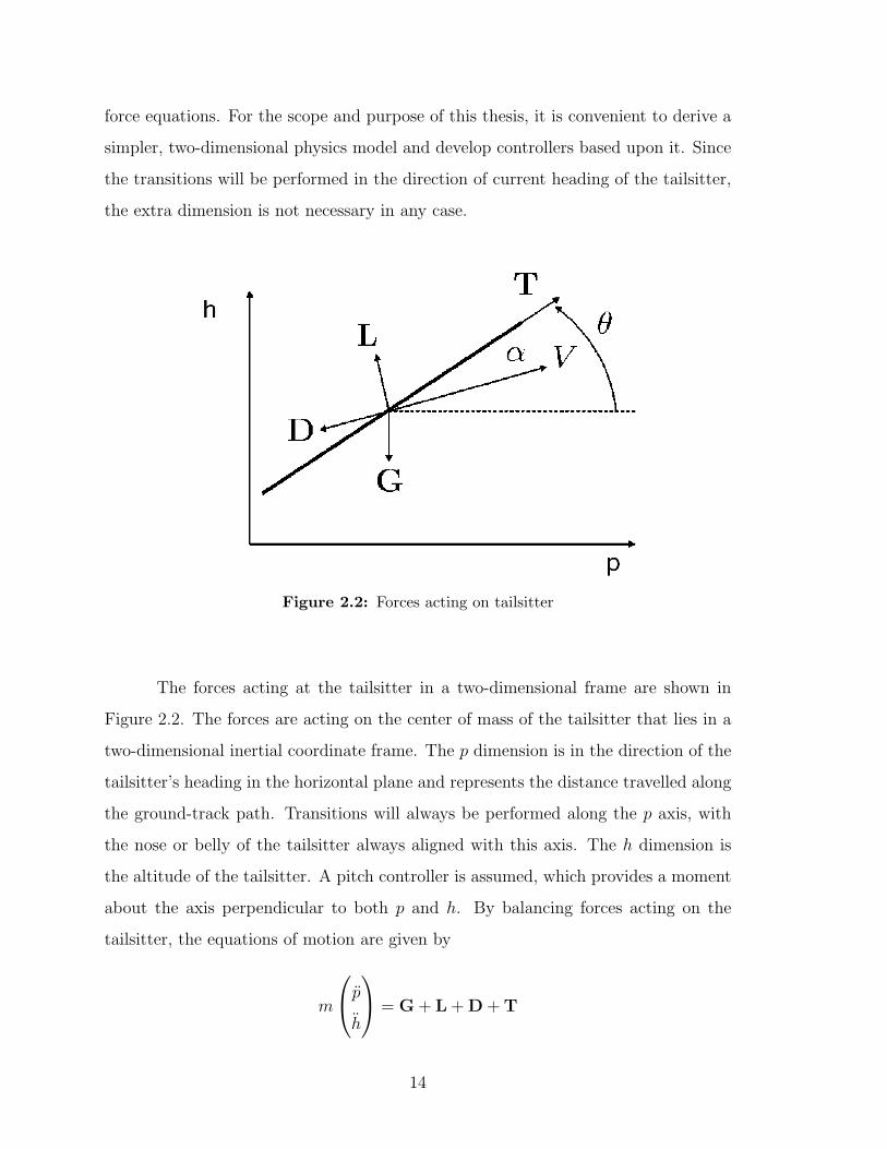
The forces acting at the tailsitter in a two-dimensional frame are shown in
Figure 2.2. The forces are acting on the center of mass of the tailsitter that lies in a
two-dimensional inertial coordinate frame. The p dimension is in the direction of the
tailsitter’s heading in the horizontal plane and represents the distance travelled along
the ground-track path. Transitions will always be performed along the p axis, with
the nose or belly of the tailsitter always aligned with this axis. The h dimension is
the altitude of the tailsitter. A pitch controller is assumed, which provides a moment
about the axis perpendicular to both p and h. By balancing forces acting on the
tailsitter, the equations of motion are given by
m
p
h
= G + L + D + T
14

and
θ = a(θc − θ)
where θ is the pitch angle, G is the force due to gravity, L is the lift force acting on
the wing, D is the drag force acting on the wing, T is the thrust produced by the
motor, and θc is the commanded pitch angle. It is assumed that a pitch controller is
available with first-order characteristics described by the positive autopilot constant
a.
In the inertial frame, the gravity vector is given by
G =
0
−mg
.
We will assume that the thrust vector is directed along the tailsitter’s body
frame x axis. Therefore, in the inertial frame we have
T = R(θ)
T
0
where R is the rotation matrix between body and inertial frames given by
R(ϕ)4=
cos ϕ − sin ϕ
sin ϕ cos ϕ
and T is the magnitude of thrust produced by the motor. We will assume that T > 0
is an input to the system.
Similarly, the lift and drag vectors are given by
L = R(θ − α)
0
L
and
D = R(θ − α)
−D
0
15
where
L =1
2ρV 2SCl(α)
is the magnitude of lift and
D =1
2ρV 2SCd(α)
is the magnitude of drag. Here Cl(α) and Cd(α) are given by Equation 2.7 and 2.8
and are shown in Figure 2.1. Combining the forces due to lift and drag gives
L + D =1
2ρV 2SR(θ − α)
−Cd(α)
Cl(α)
.
Note that the airspeed is given by
V =
√p2 + h2
and the angle of attack is given by
α = θ − tan−1
(h
p
).
Therefore θ − α = tan−1(
hp
)and
cos(θ − α) = cos
(tan−1
(h
p
))
=p√
p2 + h2
=p
V
16

and
sin(θ − α) = sin
(tan−1
(h
p
))
=h√
p2 + h2
=h
V.
Therefore
L + D =1
2ρV 2S
pV
− hV
hV
pV
−Cd
Cl
=1
2ρV S
−pCd − hCl
−hCd + pCl
and the equations of motion are given by
p
h
=
0
−g
+
1
2mρV S
−pCd − hCl
−hCd + pCl
+ R(θ)
Tm
0
(2.10)
and
θ = a(θc − θ).
2.3 Chapter Summary
Chapter 2 has given an overview of the quaternion representation used to de-
scribe the tailsitter’s attitude. The three-dimensional, quaternion-based dynamics
model will be used for simulations of controllers that will be described in later chap-
ters. A simpler, two-dimensional dynamics model was also developed. This model
will be used in the derivation of transition controllers. In Chapter 3, description
of the experimental setup and underlying navigational controllers will complete the
prerequisite discussion necessary before the development of transition controllers in
Chapter 4.
17

18
Chapter 3
Experimental Platform
This chapter describes the simulation and hardware platforms used to test
the algorithms derived to track tailsitter transition trajectories. Also, other Magicc
Lab research developed for tailsitter attitude control is described. Since the attitude
controller is prerequisite to being able to control the tailsitter during transitions with
the algorithms described in Chapter 4, it is included for completeness even though
it is not the focus of this thesis. Similarly, the navigational state machine autopilot
described in Chapter 5 for navigating between hover and level waypoints uses hover
control, level control, as well as transition control between the two modes. The hover
position controller and level flight controller are therefore briefly explained. Further
description of underlying tailsitter attitude and position controllers is found in [21].
3.1 Simulation
Each of the transition algorithms were developed and tested first in Matlab
with Simulink. The Matlab code was then converted to C and combined with the
navigational state machine code to get simulation results of the whole system at work.
The full flight path regime of hover and level waypoint following with transitions
was included. Doing this allowed the entire simulation to be tested at once. The
performance of the transition algorithms could also be seen and evaluated in the
context of residing in a larger autopilot system.
3.2 Flight Test Setup
The tailsitter test vehicle used for experimentation was the model Pogo air-
frame shown in Figure 3.1. The Pogo is modeled after the Convair Pogo mentioned in
19
the Introduction. The airframe is available commercially as a radio-controlled model
airplane kit. In the original kit purchased by the Magicc Lab, the construction ma-
terial was thin, tough styrofoam. In subsequent revisions and reworks of the Pogo,
corrugated plastic has replaced styrofoam due to its superior durability.
Figure 3.1: The Magicc Lab Pogo airframe
Prime characteristics of the Pogo airframe include very large control surfaces
and a powerful motor with large propeller attached. The motor and propeller are
able to generate a large air flow, or prop-wash over the control surfaces. In a typical
fixed-wing aircraft, aerodynamic lift forces are primarily used to keep the vehicle in
the air. When the Pogo is in hover flight, the only source of lift is generated by
the motor, and therefore the resultant thrust must be very large to keep the aircraft
aloft. The control surfaces, actuated by three electric servos typically used by radio-
controlled model airplane builders, are very large to maximize potential control in
the prop-wash region.
The Kestrel Autopilot version 2.2 shown in Figure 3.2, developed by Procerus
Technologies [22], is the heart of the Pogo. The autopilot is lightweight and compact,
measuring 5 x 10 x 1 centimeters and weighing 16 grams. The autopilot is equipped
with a Rabbit 3100 29MHz microprocessor, on which all autopilot control code is pro-
20
grammed. The autopilot also has a variety of on-board sensors, including three-axis
accelerometers and rate gyros, absolute and differential pressure sensors. Ports are
available for attaching an external GPS receiver and three-axis magnetometer. With
these sensor measurements, the autopilot is able to reasonably estimate the tailsitter’s
current state, including world frame position, altitude, attitude, and airspeed.
Figure 3.2: Kestrel Autopilot
The Kestrel Autopilot is also equipped with a communication link to the
ground station control software, Virtual Cockpit, via a 900MHz modem. The Virtual
Cockpit software, developed by the BYU Magicc Lab, displays heads-up information
about the aircraft’s current state. A satellite map of nearby terrain is also displayed,
allowing waypoints to be placed at desired locations. The waypoints and other com-
mands are uploaded and data from the aircraft can be downloaded and logged. A
bread-crumb trail of the aircraft’s trajectory is plotted.
3.3 Quaternion Attitude Control
The goal of quaternion attitude control is to adjust the tailsitter’s control
surfaces to achieve a desired attitude, as represented by the quaternion ηd. To begin
with, quaternion multiplication can be defined as
η′′ = η′ ⊗ η =
η4η
′ + η′4η − η′ × η
η′4η4 − η′η
(3.1)
21

where η′′ is the result of two successive rotations represented by η and η′ [20]. Equation
(3.1) can also be written as
η′′ = η′ ⊗ η = ηRη′ (3.2)
where
ηR =
η4 −η3 η2 η1
η3 η4 −η1 η2
−η2 η1 η4 η3
−η1 −η2 −η3 η4
.
In
ηd = ηε ⊗ ηa = ηaRηε (3.3)
ηa represents the actual attitude and ηε represents the error between the desired
and actual quaternions expressed in the aircraft’s body reference frame. Noting that
ηTRηR equals the identity matrix, the error quaternion can be written
ηε = ηaTRηd. (3.4)
The error quaternion is conveniently expressed in the aircraft body reference frame.
The aileron (δa), elevator (δe), and rudder (δr) can be used to directly control ηε and
drive Θε to zero. Therefore, for the case of zero external disturbances, stable attitude
control can be achieved by the PID-like strategy
δa
δe
δr
= k1ηε − k2Ω + k3ηεi (3.5)
where k1, k2, and k3 are diagonal gain matrices. In practice these values are gain
scheduled by dividing by the current prop-wash, creating larger gains and therefore
larger control surface deflections when the prop-wash is low. The Ω term represents
22
the current angular rates in each direction and provides a dampening effect. The
integral of quaternion error, ηεi, is used in the control to eliminate steady state error.
To provide smoother attitude tracking, the attitude control algorithm is en-
hanced by introducing a reference model quaternion. The model quaternion tracks
the desired quaternion with first-order characteristics. The model quaternion is then
used to formulate the error quaternion in Equation 3.4 rather than ηd. This provides
a smoother shift between attitudes.
The transition controllers described in Chapter 4 depend on the existence of an
underlying attitude controller. The transition controller algorithms generate desired
pitch and heading angles. These values are transformed into a desired quaternion for
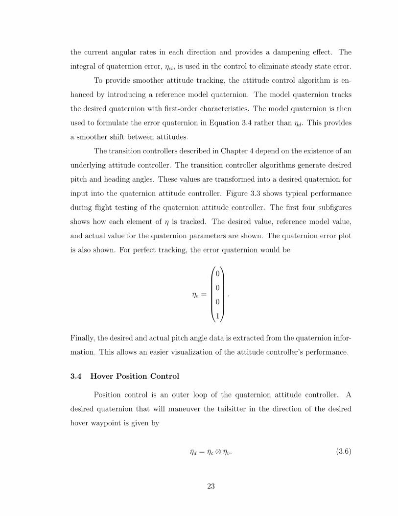
input into the quaternion attitude controller. Figure 3.3 shows typical performance
during flight testing of the quaternion attitude controller. The first four subfigures
shows how each element of η is tracked. The desired value, reference model value,
and actual value for the quaternion parameters are shown. The quaternion error plot
is also shown. For perfect tracking, the error quaternion would be
ηe =
0
0
0
1
.
Finally, the desired and actual pitch angle data is extracted from the quaternion infor-
mation. This allows an easier visualization of the attitude controller’s performance.
3.4 Hover Position Control
Position control is an outer loop of the quaternion attitude controller. A
desired quaternion that will maneuver the tailsitter in the direction of the desired
hover waypoint is given by
ηd = ηc ⊗ ηv. (3.6)
23
0 2 4 6 8 10−0.25
−0.2
−0.15
−0.1
−0.05
0
0.05
0.1
time, s
eta 1
eta1 desired
eta1 model
eta1 actual
(a) η1
0 2 4 6 8 100
0.05
0.1
0.15
0.2
0.25
0.3
0.35
time, s
eta 2
eta2 desired
eta2 model
eta2 actual
(b) η2
0 2 4 6 8 10−0.4
−0.2
0
0.2
0.4
0.6
0.8
1
time, s
eta 3
eta3 desired
eta3 model
eta3 actual
(c) η3
0 2 4 6 8 10
0.65
0.7
0.75
0.8
0.85
0.9
0.95
1
time, s
eta 4
eta4 desired
eta4 model
eta4 actual
(d) η4
0 2 4 6 8 10−0.5
0
0.5
1
time, s
quat
erni
on e
rror
eta1 error
eta2 error
eta3 error
eta4 error
(e) Error quaternion
0 2 4 6 8 100
5
10
15
20
25
30
35
40
45
time, s
deg
desired thetaactual theta
(f) θ tracking
Figure 3.3: Quaternion attitude controller performance in flight test
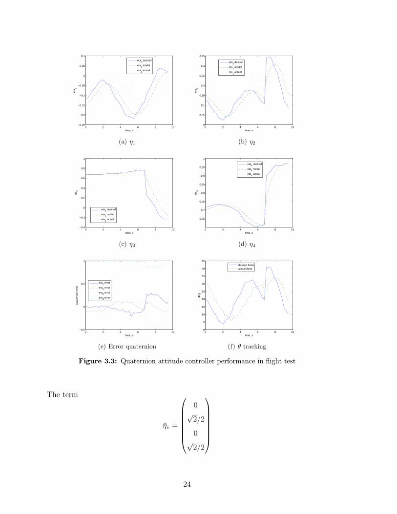
The term
ηv =
0√
2/2
0√
2/2
24
is the vertical quaternion, representing the tailsitter’s attitude with the nose of the
tailsitter pointing straight up and the belly facing North. In terms of the previously
described axes, the nose points along the negative z axis and the belly faces the
positive x axis.
The term ηc is a correction quaternion that describes the rotation needed to
tilt the nose of the aircraft in the proper direction for x-y position tracking and is
given by
ηc = ηcv ⊗ ηcp (3.7)
where ηcp is based on position error and ηcv provides dampening based on body frame
velocities. The quaternion parameters ηcp and Θcp are given by
ηcp =
0
0
1
×
(x− xd)/||ep||(y − yd)/||ep||
0
and
Θcp = k3||ep||
where k3 is a gain, xd and yd refer to the aircraft desired position, and ||ep|| is the
norm of position error
||ep|| =√
(x− xd)2 + (y − yd)2.
The quaternion components ηcv and Θcv are given by
ηcv =
0
0
1
×
w√v2+w2
v√v2+w2
0
and
Θcv = k4
√v2 + w2
25
where k4 is a gain.
Along with generating a desired quaternion for waypoint tracking, an altitude
controller also exists to allow the tailsitter to obtain and hold a given altitude while
in a hover position. Since the nose of the tailsitter generally points up in hover flight
mode, altitude can be adjusted with the throttle. First, a desired thrust command
is generated that would allow the tailsitter to descend or ascend to its commanded
altitude. A control loop that adjusts the throttle to match a desired thrust is then
used. This same throttle from thrust loop will be used by the transition controllers
in Chapter 4, which rely on being able to command and achieve a desired thrust.
In practice, descending is difficult for the tailsitter due to air flowing in the
opposing direction over the control surfaces and the decrease in prop-wash due to a
decreased throttle setting. It is therefore recommended to descend slowly, in order
to keep the throttle setting above some minimum value required to give good control
authority. With such considerations in mind, it is possible to control the tailsitter’s
altitude.
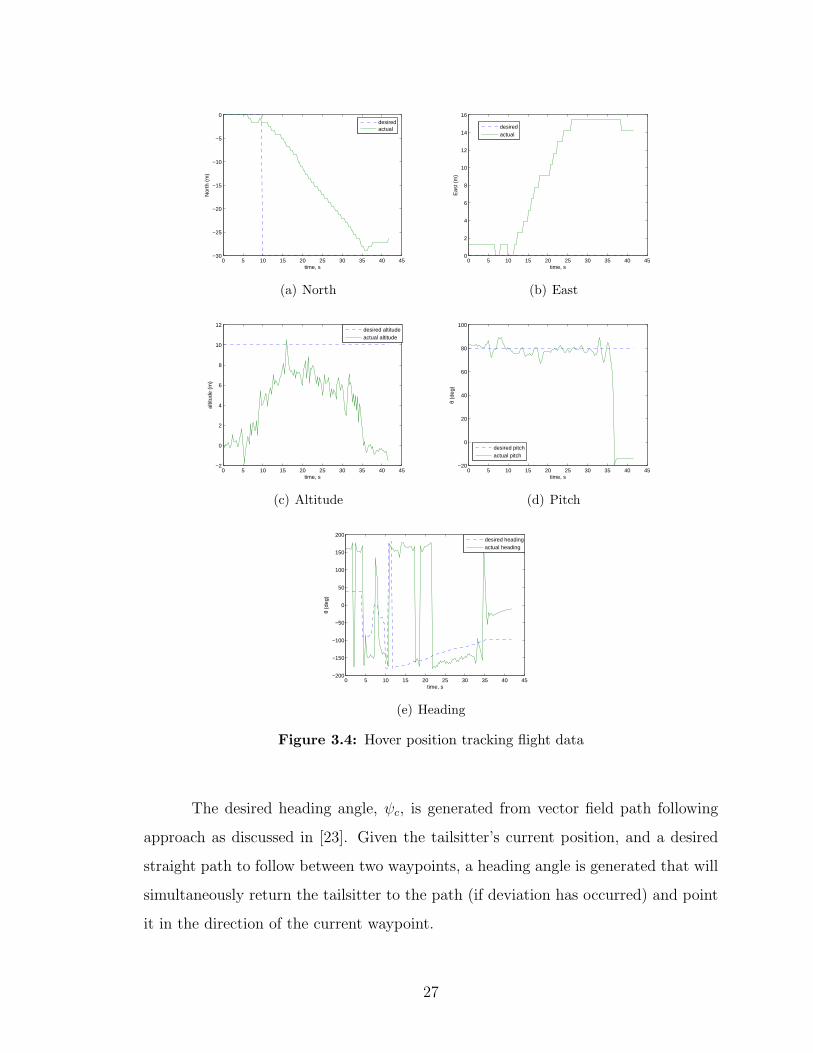
Typical performance of the hover position controller is shown in Figure 3.4.
In this experiment, the tailsitter hovers at (0,0) and then is commanded to hover to
a point 30 meters to the south. Also, the altitude is controlled by throttle and is set
to a desired value of 10 meters. The tailsitter begins on the ground and takes off at
about t = 10 seconds. It is seen that the tailsitter does move south 30 meters, but
also drifts to the east a considerable distance, which is caused by wind. Due its large
wing area and lightweight construction materials, the tailsitter is very susceptible to
wind, especially while in a hover position. The hover controller can compensate for
some wind by tilting the nose of the tailsitter into the wind, but for this flight test
this was not enough to prevent drifting in the direction of wind.
3.5 Level Flight Control
The level flight controller also has the quaternion attitude controller as an
inner loop. Desired Euler angles θc and ψc are generated and converted to a command
quaternion by Equation 2.3. The roll angle, φc is left at zero for level flight control.
26
0 5 10 15 20 25 30 35 40 45−30
−25
−20
−15
−10
−5
0
time, s
Nor
th (
m)
desiredactual
(a) North
0 5 10 15 20 25 30 35 40 450
2
4
6
8
10
12
14
16
time, s
Eas
t (m
)
desiredactual
(b) East
0 5 10 15 20 25 30 35 40 45−2
0
2
4
6
8
10
12
time, s
altit
ude
(m)
desired altitudeactual altitude
(c) Altitude
0 5 10 15 20 25 30 35 40 45−20
0
20
40
60
80
100
time, s
θ (d
eg)
desired pitchactual pitch
(d) Pitch
0 5 10 15 20 25 30 35 40 45−200
−150
−100
−50
0
50
100
150
200
time, s
θ (d
eg)
desired headingactual heading
(e) Heading
Figure 3.4: Hover position tracking flight data
The desired heading angle, ψc, is generated from vector field path following
approach as discussed in [23]. Given the tailsitter’s current position, and a desired
straight path to follow between two waypoints, a heading angle is generated that will
simultaneously return the tailsitter to the path (if deviation has occurred) and point
it in the direction of the current waypoint.
27
Pitch angle, θc, and the throttle setting are generated to track desired altitude.
When within a window of the desired altitude, the pitch angle is controlled with a
feed-forward loop using altitude error, and the throttle is used to maintain airspeed.
Above the altitude window, pitch is controlled to maintain airspeed and throttle is
set to a designated low setting. Below the altitude window, the pitch-from-airspeed
loop is also in effect, but throttle is turned on to full. With this scheme, good altitude
tracking in level flight is possible.
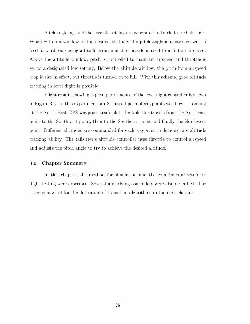
Flight results showing typical performance of the level flight controller is shown
in Figure 3.5. In this experiment, an X-shaped path of waypoints was flown. Looking
at the North-East GPS waypoint track plot, the tailsitter travels from the Northeast
point to the Southwest point, then to the Southeast point and finally the Northwest
point. Different altitudes are commanded for each waypoint to demonstrate altitude
tracking ability. The tailsitter’s altitude controller uses throttle to control airspeed
and adjusts the pitch angle to try to achieve the desired altitude.
3.6 Chapter Summary
In this chapter, the method for simulation and the experimental setup for
flight testing were described. Several underlying controllers were also described. The
stage is now set for the derivation of transition algorithms in the next chapter.
28
−140 −120 −100 −80 −60 −40 −20 0 20−140
−120
−100
−80
−60
−40
−20
0
20
40
60
East (m)
Nor
th (
m)
(a) N-E waypoints
0 10 20 30 40 50 600
5
10
15
20
25
30
35
40
45
time, s
altit
ude
(m)
desired altitudeactual altitude
(b) Altitude
0 10 20 30 40 50 60−2
0
2
4
6
8
10
12
time, s
airs
peed
(m
/sec
)
desired airspeedactual airspeed
(c) Airspeed
0 10 20 30 40 50 60−40
−30
−20
−10
0
10
20
30
40
50
time, s
φ (d
eg)
desired rollactual roll
(d) φ
0 10 20 30 40 50 60−20
−10
0
10
20
30
40
50
60
time, s
θ (d
eg)
desired pitchactual pitch
(e) θ
0 10 20 30 40 50 60−200
−150
−100
−50
0
50
100
150
200
time, s
ψ (
deg)
desired headingactual heading
(f) ψ
Figure 3.5: Level waypoint tracking flight data
29

30
Chapter 4
Trajectory Tracking Algorithms
In this chapter, a method for creating desired two-dimensional trajectories for
tailsitter transitions is presented. Also, three methods for following that trajectory
through each type of maneuver (hover-to-level and level-to-hover) are given. Simula-
tion results and actual flight test results are also given for each of the three methods.
4.1 Desired Trajectories
The goal of trajectory design is to develop trajectories that will be followed
during each type of transition maneuver. The trajectories should be simple and easy
to follow. Trajectory design is performed in a two-dimensional world frame. The
parameter p represents the distance travelled in a line along the current heading.
Altitude is referred to as h. The trajectories are all time based, with t being the
current time and t = 0 at the start of the transition.
In practice, a transition will occur between a level waypoint and a hover way-
point, or vice versa. The straight line path between the two waypoints is the heading
along which the maneuver is performed. The point along that path that the maneuver
begins is dictated by a higher level command module that is described in Chapter 5.
A desirable transition will guide the tailsitter in between an initial position,
(p0, h0), and a final desired position, (pf , hf ). For a hover-to-level transition, the tail-
sitter will be in a hover position at (p0, h0) and be flying level with a constant velocity
at (pf , hf ), as shown in Figure 4.1. For a level-to-hover transition, the tailsitter will
be flying level with some initial velocity at (p0, h0) and hovering at (pf , hf ), as shown
in Figure 4.2.
31
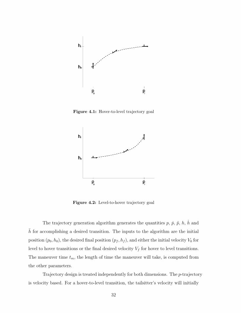
Figure 4.1: Hover-to-level trajectory goal
Figure 4.2: Level-to-hover trajectory goal
The trajectory generation algorithm generates the quantities p, p, p, h, h and
h for accomplishing a desired transition. The inputs to the algorithm are the initial
position (p0, h0), the desired final position (pf , hf ), and either the initial velocity V0 for
level to hover transitions or the final desired velocity Vf for hover to level transitions.
The maneuver time tm, the length of time the maneuver will take, is computed from
the other parameters.
Trajectory design is treated independently for both dimensions. The p-trajectory
is velocity based. For a hover-to-level transition, the tailsitter’s velocity will initially
32

be zero and will need to increase to Vf when it is in level flight. For a level-to-hover
transition, the velocity will initially be V0 and will then go to zero as the tailsitter
assumes a hover position. Trajectories in the p direction are developed with this goal
in mind and are given by
pd =
Vf
tm, t ≤ tm
0, otherwise
pd =
Vf
tmt, t ≤ tm
Vf , otherwise
pd =
Vf
2tmt2 + p0, t ≤ tm
Vf (t− tm) + Vftm2
, otherwise
where
tm =2(pf − p0)
Vf
for a hover-to-level transition and
pd =
− V0
tm, t ≤ tm
0, otherwise
pd =
− V0
tmt + V0, t ≤ tm
0, otherwise
pd =
− V0
2tmt2 + V0t + p0, t ≤ tm
− V0
2tmt2m + V0tm + p0, otherwise
where
tm =2(pf − p0)
V0
33

for a level-to-hover transition.
0 5 10 15 20 25 30 35 40
0
0.1
0.2
0.3
0.4
0.5
s
pd d
dot
(a) Desired p for hover to level
0 5 10 15 20 25 30 35 40
−0.5
−0.4
−0.3
−0.2
−0.1
0
s
pd d
dot
(b) Desired p for level to hover
0 5 10 15 20 25 30 35 400
1
2
3
4
5
6
7
8
9
10
11
s
pd d
ot
(c) Desired p for hover to level
0 5 10 15 20 25 30 35 40−1
0
1
2
3
4
5
6
7
8
9
10
s
pd d
ot
(d) Desired p for level to hover
0 5 10 15 20 25 30 35 400
50
100
150
200
250
300
s
pd
(e) Desired p for hover to level
0 5 10 15 20 25 30 35 400
10
20
30
40
50
60
70
80
90
100
s
pd
(f) Desired p for level to hover
Figure 4.3: Desired p-trajectories
34
For desired trajectories in the h dimension a different approach is desired. For
both transition types, we desire a smooth shift from a constant altitude to another
constant altitude. This can be achieved with the use of sigmoid functions. For both
hover to level and level to hover transitions, the desired trajectories are given by
hd =hf − h0
1 + e−k(t− tm2
)+ h0,
hd = k(hf − h0)ekt+( tm
2)k
(ekt + etmk2 )2
,
and
hd =−k2(hf − h0)(e
kt − etmk2 )ekt+tm
k2
(ekt + etmk2 )3
.
In these equations, k is a constant that determines how quickly the desired
altitude trajectory curves arrive at their final value. The length of time of the ma-
neuver is determined by the distance along the path, from p0 to pf , and is calculated
in the discussion on desired p trajectories. Once the value of tm is determined, it is
used in sigmoid functions to develop smooth h trajectories.
The desired p-trajectories are shown in Figure 4.3. Desired h-trajectories are
shown in Figure 4.4. For both maneuvers, the input parameters are (p0, h0) = (0, 50)
and (pf , hf ) = (100, 60).
4.2 Simple Controller
It is desirable to develop a controller that will successfully follow the trajec-
tories generated in Section 4.1. Sections 4.3 and 4.4 both describe methods that will
follow the trajectories. The controller described in this section, however, will suc-
cessfully perform a transition, but only follows the desired h trajectory. This type
of transition is useful when the lateral distance travelled is not as important as per-
35
0 5 10 15 20 25 30 35 4050
51
52
53
54
55
56
57
58
59
60
61
s
hd(a) Desired h for both transition types
0 5 10 15 20 25 30 35 400
0.1
0.2
0.3
0.4
0.5
0.6
0.7
0.8
s
hd d
ot
(b) Desired h for both transition types
0 5 10 15 20 25 30 35 40−0.1
−0.08
−0.06
−0.04
−0.02
0
0.02
0.04
0.06
0.08
0.1
s
hd d
dot
(c) Desired h for both transition types
Figure 4.4: Desired h-trajectories
forming a transition with little altitude deviation. For instance, if the tailsitter were
equipped with some sensor that could detect a nearby wall directly in the level flight
path, a quick level-to-hover transition could be commanded. Furthermore, the de-
velopment of a simple controller will provide a baseline for judging performance and
other issues with the other two, more complex controllers.
36
When the maneuver begins with the simple controller, a desired quaternion is
generated from Equation 2.3 with φ = 0, ψ being the heading between the previous
and current waypoint, and θ being zero for a hover-to-level transition or ninety degrees
for a level-to-hover transition. This is used as the desired quaternion in the quaternion
attitude controller described in Section 3.3 and in [21]. While the tailsitter is making
the transition, the throttle from altitude control loop is enabled, allowing desired
altitude to be tracked. This control loop generates a desired thrust to follow to
achieve a desired altitude. The desired thrust is tracked by adjusting the throttle.
4.3 Feedback Linearization Controller
Feedback linearization is a technique of controlling nonlinear systems by trans-
forming them into an equivalent linear system [24]. Fortunately for the case of tail-
sitter dynamics, Equation 2.10 is already in normal form, with the control inputs T
and θ separated from the nonlinearities. The feedback linearization controller relies
on knowledge of the aerodynamic model to derive a controller to track both p and h
trajectories through transition maneuvers. First, define position error as
p = p− pd
and
h = h− hd.
Then acceleration error is
¨p
¨h
=
p− pd
h− hd
=
ρS2m
√p2 + h2(−pCd − hCl) + T
mcos θ − pd
−g + ρS2m
√p2 + h2(−hCd + pCl) + T
msin θ − hd
.
37
The control input we will define as
U4=
Tm
cos θ
Tm
sin θ
= U1 + U2
where U1 will be used to cancel nonlinearities from the system and U2 is a pseudo-
input that will be selected to drive tracking error to zero. By selecting U1 as
U1 =
− ρS
2m
√p2 + h2(−pCd − hCl)
g − ρS2m
√p2 + h2(−hCd + pCl)
the system is linearized and now becomes
¨p
¨h
= U2 −
pd
hd
.
To track the desired p and h trajectories with second order characteristics, it is
desirable for
¨p = −kdp˙p− kppp
and
¨h = −kdh˙h− kphh
where kdp, kpp, kdh, and kph are tunable gains.
To achieve this, let
U2 =
−kdp
˙p− kppp + pd
−kdh˙h− kphh + hd
.
The control input is then
Tm
cos θ
Tm
sin θ
= U1 + U2 =
− ρS
2m
√p2 + h2(−pCd − hCl)− kdp
˙p− kppp + pd
g − ρS2m
√p2 + h2(−hCd + pCl)− kdh
˙h− kphh + hd
.
38
To be able to eventually command thrust values and pitch commands, it is necessary
get independent expressions for T and θ. We find it convenient to redefine the rows
of the input vector as
F14= − ρS
2m
√p2 + h2(−pCd − hCl)− kdp
˙p− kppp + pd
and
F24= g − ρS
2m
√p2 + h2(−hCd + pCl)− kdh
˙h− kphh + hd
resulting in the expressionsT
mcos θ = F1 (4.1)
andT
msin θ = F2. (4.2)
By squaring both of these equations and adding the results together, we have
T 2
m2= F 2
1 + F 22
and therefore the value for thrust is
T = m√
F 21 + F 2
2 .
If we divide Equation 4.2 by Equation 4.1,
Tm
sin θTm
cos θ=
F2
F1
and
tan θ =F2
F1
so
θ = tan−1 F2
F1
.
39
We now have command values for thrust and θ. In practice, the commanded
pitch value along with the heading angle along which the maneuver is to be performed
is converted to a quaternion using Equation 2.3. This quaternion is then used as the
desired quaternion in the quaternion attitude controller from Section 3.3. The throttle
command T is fed to the throttle from the thrust feedback control loop, which adjusts
the throttle setting to effect a desired thrust.
The feedback linearization controller requires knowledge of several parameters
that are not known or measured accurately on the tailsitter. These parameters pri-
marily include Cl and Cd, which are given by Equations 2.7 and 2.8. This controller’s
performance is therefore expected to be greatly affected by how well the true values
of these parameters are known.
4.4 Adaptive Controller
In the feedback linearization example, several parameters that are not typically
known were made available to the controller. In this section, a model reference
adaptive controller (MRAC) is described which requires knowledge of only m, g,
state information p, p, h and h, and desired trajectories for pd and hd. We will then
eliminate the need to require knowledge of Cl and Cd in order to successfully track a
desired trajectory.
4.4.1 Lyapunov Stability
Derivation of the adaptive control method relies on Lyapunov stability theory,
discussed in [24], which provides conditions to prove a system’s stability. First a
Lyapunov function V (x) is chosen, where x denotes the state variables that need to
be driven to zero. In the case to be described below, x is the trajectory tracking error,
that we would like to drive to zero. The choice of V (x) must adhere to the following
rules:
1. V (0) = 0,
2. V (x) > 0, or in other words, V (x) is positive definite,
40
3. V (x) is continuously differentiable.
If V (x) meets these criteria and V (x) < 0 for x 6= 0, or in other words, V (x) is
negative definite, then x → 0 asymptotically.
The adaptive control method described in this section will develop a Lyapunov
function based on the error in tracking desired trajectories. Then, with the addition
of a proper parameter estimation scheme, it will be shown that the derivative of the
Lyapunov function is negative definite and therefore the error in trajectory tracking
will go to zero.
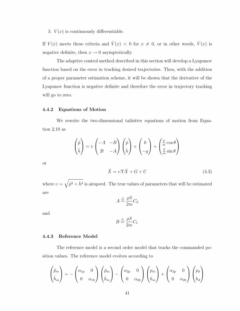
4.4.2 Equations of Motion
We rewrite the two-dimensional tailsitter equations of motion from Equa-
tion 2.10 as
p
h
= υ
−A −B
B −A
p
h
+
0
−g
+
Tm
cos θ
Tm
sin θ
or
X = υΥX + G + U (4.3)
where υ =
√p2 + h2 is airspeed. The true values of parameters that will be estimated
are
A4=
ρS
2mCd
and
B4=
ρS
2mCl.
4.4.3 Reference Model
The reference model is a second order model that tracks the commanded po-
sition values. The reference model evolves according to
pm
hm
= −
α1p 0
0 α1h
pm
hm
−
α2p 0
0 α2h
pm
hm
+
α2p 0
0 α2h
pd
hd
41
or
R = −α1R− α2R + α2Rc (4.4)
where α values are tunable gains and pd, hd are desired trajectory values.
4.4.4 Controller Derivation
The adaptive controller is given in Theorem 4.1. The proof is used to show
that with adaptive parameter estimation, the position error
X4= X −R
and the velocity error
˙X = X − R
are both asymptotically stable.
Theorem 4.1 If the estimates of A and B, called A and B, are updated according
to
˙A = γ1
√p2 + h2(−p ˙p− h ˙h)
and
˙B = γ2
√p2 + h2(−h ˙p + p ˙h)
where γ1 and γ2 are gains, and the control input is given as
U = −k ˙X − X − υΥX −G− α1R− α2R + α2Rc
where the reference model propagates according to Equation 4.4, then
˙X → 0
and
X → 0
42
asymptotically.
Proof: Consider the Lyapunov function candidate
V =1
2XT X +
1
2˙XT ˙X +
1
2γξT ξ (4.5)
where
ξ = ξ − ξ
is the difference between actual and estimated A and B parameters and is given by
ξ =
A
B
=
A
B
−
A
B
and γ is the vector of adaptive control gains
γ =
γ1
γ2
.
The time derivative of (4.5) can be shown to be
V = ˙XT X + ˙XT ¨X +1
γ˙ξT ξ (4.6)
where
¨X = X − R.
Replacing ¨X in Equation 4.6 with X from Equation 4.3 and R from Equation 4.4
results in
V = ˙XT (X + υΥX + G + U + α1R + α2R− α2Rc) +1
γ˙ξT ξ.
Substituting U with the expression given in the statement of Theorem 4.1 gives
V = −k ˙XT ˙X + υ ˙XT ΥX +1
γ˙ξT ˙ξ (4.7)
43
where
Υ4= Υ− Υ
is the difference between actual and estimated parameters A and B. Equation 4.7
may be rewritten as
V = −k ˙XT ˙X + υ ˙XT Zξ +1
γ˙ξT ξ
where
Z4=
−p −h
−h p
and
˙ξ = ξ − ˙ξ.
We assume that ξ is slowing varying enough that ξ may be treated as zero. Then the
Lyapunov function derivative becomes
V = −k ˙XT ˙X + υ ˙XT Zξ +1
γ˙ξT ξ.
By choosing the adaptive parameter update law as given in the statement of Theo-
rem 4.1, or in other terms
˙ξT = γυ ˙XT Z
then
V = −k ˙XT ˙X. (4.8)
Since V is negative definite, ˙X → 0 by the theory of Lyapunov. LaSalle’s Invariance
Principle [24] will be used to show that X → 0.
Let the set E be defined as
E4=
X
˙X
ξ
: V = 0
.
44
The derivative of the Lyapunov function is only 0 where ˙X = 0, so
E =
X
˙X
ξ
: ˙X = 0
.
Let M be the largest invariant set in E. Then
X
˙X
ξ
∈ M ⇒ ˙X(t) = 0 ∀ t.
Therefore if X(0) = 0, or in other words if the reference model begins as the current
value of X, then
X(t) = 0 ∀ t
and X is asymptotically stable.
Although using an adaptive controller is beneficial in that knowledge of system
parameters is not required, a host of new gains used in the algorithm are introduced
which must be then be tuned primarily by trial and error. In general, each of these
gains has a specific effect. The gain α determines how closely the reference model
tracks the desired trajectory, γ controls how fast the estimated parameters adapt,
and k determines how fast the actual values converge to the reference model.
4.5 Simulation Results
Each of the controllers was simulated in Matlab Simulink for both a hover-
to-level transition and a level-to-hover transition. The physics model used in the
simulations is described in Section 2.1.
45
4.5.1 Simple Controller Simulations
The results from the simple controller simulation are seen in Figure 4.5 for
hover-to-level and Figure 4.6 for level-to- hover. As described in Section 4.2, no
effort is being made to track the p trajectory. Although there are some deviations in
tracking the h trajectory, the controller approaches the final desired altitude for both
transition types. This controller’s primary benefit is its simplicity. When a transition
is desired but trajectory tracking is not a high priority, then the simple controller
should perform nicely.
0 5 10 15 20 25 30 35 400
50
100
150
200
250
300
350
400
time, sec
p, m
eter
s
pd
p
(a) p
0 5 10 15 20 25 30 35 4048
50
52
54
56
58
60
62
time, sec
h, m
eter
s
hd
h
(b) h
0 5 10 15 20 25 30 35 400
2
4
6
8
10
12
14
16
time, sec
thru
std, N
(c) thrust
0 5 10 15 20 25 30 35 400
0.2
0.4
0.6
0.8
1
1.2
1.4
1.6
time, sec
thet
a d, rad
(d) θ
Figure 4.5: Simple controller hover-to-level trajectory tracking in simulation
46
0 5 10 15 20 25 30 35 400
50
100
150
200
250
time, sec
p, m
eter
s
pd
p
(a) p
0 5 10 15 20 25 30 35 4048
50
52
54
56
58
60
62
time, sec
h, m
eter
s
hd
h
(b) h
0 5 10 15 20 25 30 35 400
2
4
6
8
10
12
14
16
time, sec
thru
std, N
(c) thrust
0 5 10 15 20 25 30 35 400
0.2
0.4
0.6
0.8
1
1.2
1.4
1.6
time, sec
thet
a d, rad
(d) θ
Figure 4.6: Simple controller level-to-hover trajectory tracking in simulation
47

4.5.2 Feedback Linearization Controller Simulations
Figure 4.7 shows the results of the feedback linearization controller simulation
for a hover-to-level transition. Level-to-hover transition results are shown in Fig-
ure 4.8. As is seen, the feedback linearization controller works very well for tracking
both trajectories during the entire course of the maneuver. During the level-to-hover
transition, it is seen that around t = 30 seconds a slight deviation in p tracking oc-
curs. To restore the tailsitter to the proper trajectory, a corresponding dip in pitch
can be seen. The controller pitches down the tailsitter in order to gain velocity in the
p direction and correct the deviation. When the tailsitter is once again tracking, the
tailsitter pitches back up to a vertical position.
0 5 10 15 20 25 30 35 400
50
100
150
200
250
300
350
time, sec
p, m
eter
s
pd
p
(a) p
0 5 10 15 20 25 30 35 4048
50
52
54
56
58
60
62
time, sec
h, m
eter
s
hd
h
(b) h
0 5 10 15 20 25 30 35 402
4
6
8
10
12
14
16
18
time, sec
thru
std, N
(c) thrust
0 5 10 15 20 25 30 35 400.4
0.6
0.8
1
1.2
1.4
1.6
1.8
time, sec
thet
a d, rad
(d) θ
Figure 4.7: Feedback linearization controller hover-to-level trajectory tracking in sim-ulation
48
0 5 10 15 20 25 30 35 400
20
40
60
80
100
120
time, sec
p, m
eter
s
pd
p
(a) p
0 5 10 15 20 25 30 35 4050
51
52
53
54
55
56
57
58
59
60
time, sec
h, m
eter
s
hd
h
(b) h
0 5 10 15 20 25 30 35 402
4
6
8
10
12
14
16
time, sec
thru
std, N
(c) thrust
0 5 10 15 20 25 30 35 400.4
0.6
0.8
1
1.2
1.4
1.6
1.8
time, sec
thet
a d, rad
(d) θ
Figure 4.8: Feedback linearization controller level-to-hover trajectory tracking in sim-ulation
49
4.5.3 Adaptive Controller Simulations
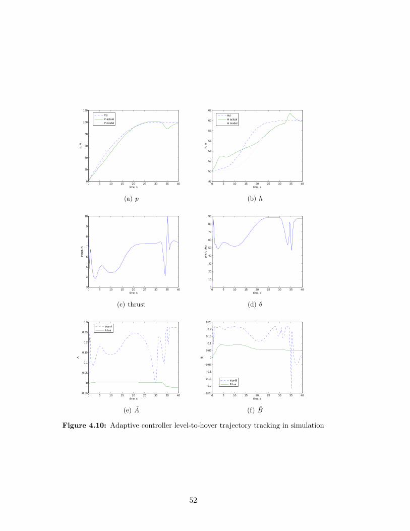
Adaptive controller simulation results are seen in Figure 4.9 and Figure 4.10
for hover-to-level transition results and level-to-hover transition results, respectively.
Simulation results show favorable trajectory tracking for both p and h dimensions
with a maximum deviation of about 7 m in p and 4 m in h. The adaptively estimated
parameters A and B are also plotted and can be seen to adapt to changing conditions
as the tailsitter flies through its transitions. The true values of A and B are also
plotted. The estimated parameters are not guaranteed to track the actual values of
these parameters and are not seen to do so, although the estimates do generally move
in the same direction as the actual values.
During the first moments of the level to hover transition, there is poor tracking
as the estimated parameters change rapidly. The result is a large spike in both desired
thrust and desired pitch angle. Once the adaptive algorithm has been running for a
few iterations, the parameters stabilize resulting in a smoother transition in thrust
and pitch angle. This effect will be minimized in actual implementation by choosing
gains appropriately.
50

0 5 10 15 20 25 30 35 400
20
40
60
80
100
120
140
160
180
time, s
p, m
PdP actualP model
(a) p
0 5 10 15 20 25 30 35 4050
55
60
65
time, s
h, m
HdH actualH model
(b) h
5 10 15 20 25 30 350
1
2
3
4
5
6
7
8
time, s
thru
st, N
(c) thrust
0 5 10 15 20 25 30 35 4020
30
40
50
60
70
80
90
time, s
pitc
h, d
eg
(d) θ
0 5 10 15 20 25 30 35 40−0.05
0
0.05
0.1
0.15
0.2
0.25
0.3
time, s
A
true AA hat
(e) A
0 5 10 15 20 25 30 35 40−0.25
−0.2
−0.15
−0.1
−0.05
0
0.05
0.1
0.15
0.2
0.25
time, s
B
true BB hat
(f) B
Figure 4.9: Adaptive controller hover-to-level trajectory tracking in simulation
51
0 5 10 15 20 25 30 35 400
20
40
60
80
100
120
time, s
p, m
PdP actualP model
(a) p
0 5 10 15 20 25 30 35 4048
50
52
54
56
58
60
62
time, s
h, m
HdH actualH model
(b) h
0 5 10 15 20 25 30 35 403
4
5
6
7
8
9
10
time, s
thru
st, N
(c) thrust
0 5 10 15 20 25 30 35 400
10
20
30
40
50
60
70
80
90
time, s
pitc
h, d
eg
(d) θ
0 5 10 15 20 25 30 35 40−0.05
0
0.05
0.1
0.15
0.2
0.25
0.3
time, s
A
true AA hat
(e) A
0 5 10 15 20 25 30 35 40−0.25
−0.2
−0.15
−0.1
−0.05
0
0.05
0.1
0.15
0.2
0.25
time, s
B
true BB hat
(f) B
Figure 4.10: Adaptive controller level-to-hover trajectory tracking in simulation
52
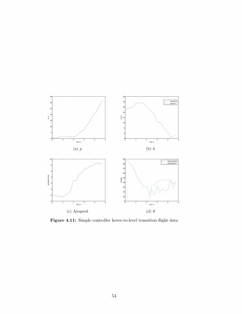
4.6 Flight Test Results
Results from flight testing show the algorithms working, but performance is
only satisfactory. Trajectory tracking is not as good as simulation results. This is
attributable to a number of factors. Primarily, the reality of sensor noise and lag
hurts performance the most. In particular, GPS, which is used to measure position
and velocities, is known to be inaccurate as well as time delayed. Also, GPS updates
occur only a few times per second. Performance would undoubtedly be improved if
GPS readings were improved and the frequency of updates increased.
Along with sub-par sensors, the other factors contributing to deviations in
the flight results are the characteristics of the underlying controllers described in
Chapter 3. Both feedback linearization and adaptive controllers depend on being
able to command a desired pitch angle and desired thrust command. The quaternion
attitude controller and thrust controller are not able to perfectly match the desired
commands. Improvements to trajectory tracking through transitions will be seen as
these controllers are improved.
4.6.1 Simple Controller Flight Results
In actual flight on the tailsitter, the simple controller is able to complete the
desired transitions very quickly. For both types of maneuvers, however, altitude devi-
ation is very large, approaching 10 meters or more. For the hover-to-level transition,
shown in Figure 4.11, a drop in altitude is seen while for the level-to-hover transi-
tion, shown in Figure 4.12, altitude increases by about this same amount. During
the transitions, the altitude hold loop is enabled, which uses the throttle to achieve
a thrust that should balance the weight of the tailsitter while in a hover position.
For the time the tailsitter is taken out of a hover position by the simple controller,
the altitude controller has difficulty maintaining altitude with just the throttle. Also,
limitations of the thrust tracking controller must also be taken into account to explain
the evident altitude deviations.
53
0 1 2 3 4 50
5
10
15
20
25
30
35
time, s
p, m
(a) p
0 1 2 3 4 54
6
8
10
12
14
16
18
20
time, s
h (m
)
desired hactual h
(b) h
0 1 2 3 4 5−4
−2
0
2
4
6
8
10
time, s
airs
peed
(m
/s)
(c) Airspeed
0 1 2 3 4 50
10
20
30
40
50
60
70
80
90
time, s
θ (d
eg)
desired pitchactual pitch
(d) θ
Figure 4.11: Simple controller hover-to-level transition flight data
54
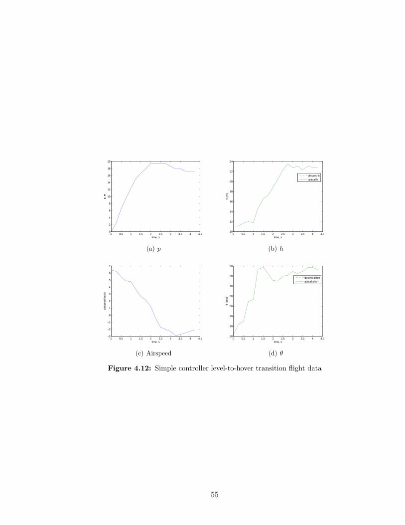
0 0.5 1 1.5 2 2.5 3 3.5 4 4.50
2
4
6
8
10
12
14
16
18
20
time, s
p, m
(a) p
0 0.5 1 1.5 2 2.5 3 3.5 4 4.510
12
14
16
18
20
22
24
time, s
h (m
)
desired hactual h
(b) h
0 0.5 1 1.5 2 2.5 3 3.5 4 4.5−3
−2
−1
0
1
2
3
4
5
6
7
time, s
airs
peed
(m
/s)
(c) Airspeed
0 0.5 1 1.5 2 2.5 3 3.5 4 4.520
30
40
50
60
70
80
90
time, s
θ (d
eg)
desired pitchactual pitch
(d) θ
Figure 4.12: Simple controller level-to-hover transition flight data
55
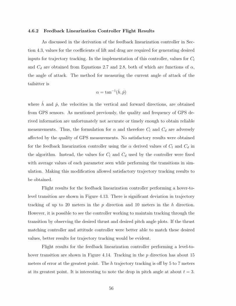
4.6.2 Feedback Linearization Controller Flight Results
As discussed in the derivation of the feedback linearization controller in Sec-
tion 4.3, values for the coefficients of lift and drag are required for generating desired
inputs for trajectory tracking. In the implementation of this controller, values for Cl
and Cd are obtained from Equations 2.7 and 2.8, both of which are functions of α,
the angle of attack. The method for measuring the current angle of attack of the
tailsitter is
α = tan−1(h, p)
where h and p, the velocities in the vertical and forward directions, are obtained
from GPS sensors. As mentioned previously, the quality and frequency of GPS de-
rived information are unfortunately not accurate or timely enough to obtain reliable
measurements. Thus, the formulation for α and therefore Cl and Cd are adversely
affected by the quality of GPS measurements. No satisfactory results were obtained
for the feedback linearization controller using the α derived values of Cl and Cd in
the algorithm. Instead, the values for Cl and Cd used by the controller were fixed
with average values of each parameter seen while performing the transitions in sim-
ulation. Making this modification allowed satisfactory trajectory tracking results to
be obtained.
Flight results for the feedback linearization controller performing a hover-to-
level transition are shown in Figure 4.13. There is significant deviation in trajectory
tracking of up to 20 meters in the p direction and 10 meters in the h direction.
However, it is possible to see the controller working to maintain tracking through the
transition by observing the desired thrust and desired pitch angle plots. If the thrust
matching controller and attitude controller were better able to match these desired
values, better results for trajectory tracking would be evident.
Flight results for the feedback linearization controller performing a level-to-
hover transition are shown in Figure 4.14. Tracking in the p direction has about 15
meters of error at the greatest point. The h trajectory tracking is off by 5 to 7 meters
at its greatest point. It is interesting to note the drop in pitch angle at about t = 3.
56
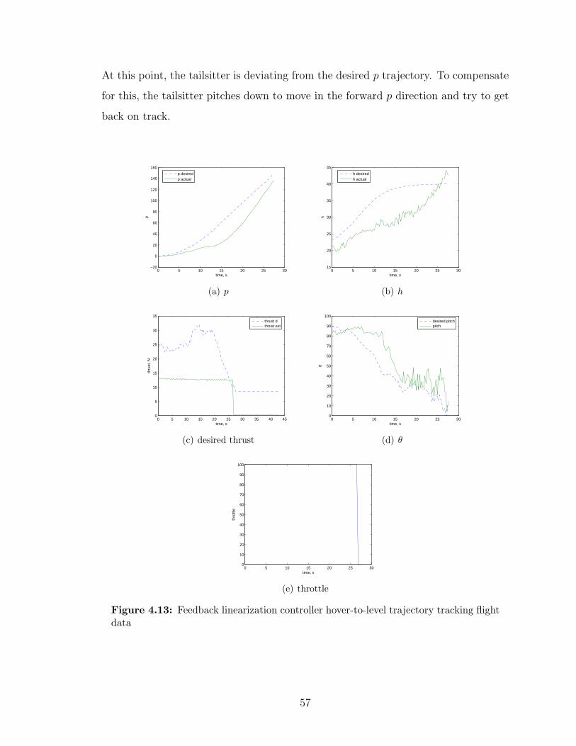
At this point, the tailsitter is deviating from the desired p trajectory. To compensate
for this, the tailsitter pitches down to move in the forward p direction and try to get
back on track.
0 5 10 15 20 25 30−20
0
20
40
60
80
100
120
140
160
time, s
p
p desiredp actual
(a) p
0 5 10 15 20 25 3015
20
25
30
35
40
45
time, s
h
h desiredh actual
(b) h
0 5 10 15 20 25 30 35 40 450
5
10
15
20
25
30
35
time, s
thru
st, N
thrust dthrust est
(c) desired thrust
0 5 10 15 20 25 300
10
20
30
40
50
60
70
80
90
100
time, s
θdesired pitchpitch
(d) θ
0 5 10 15 20 25 300
10
20
30
40
50
60
70
80
90
100
time, s
thro
ttle
(e) throttle
Figure 4.13: Feedback linearization controller hover-to-level trajectory tracking flightdata
57
0 1 2 3 4 5 6 7 8 90
5
10
15
20
25
30
35
40
45
50
time, s
m
PdP actual
(a) p
0 1 2 3 4 5 6 7 8 930
35
40
45
50
55
time, s
m
HdH actual
(b) h
0 1 2 3 4 5 6 7 8 90
5
10
15
20
25
30
time, s
Des
ired
thru
st, N
(c) desired thrust
0 1 2 3 4 5 6 7 8 9−10
0
10
20
30
40
50
60
70
80
90
time, s
deg
des thetatheta
(d) θ
0 1 2 3 4 5 6 7 8 940
50
60
70
80
90
100
time, s
% th
rottl
e
(e) throttle
Figure 4.14: Feedback linearization controller level-to-hover trajectory tracking flightdata
58
4.6.3 Adaptive Controller Flight Results
Flight results of a hover to level transition using the adaptive controller are
shown in Figure 4.15. Tracking in the p direction is good at the start of the maneuver
but grows to nearly 40 meters at the end. Altitude tracking is much better, with
deviations of less than 3 meters until the end of the transition, when error reaches
about 10 meters. These errors are likely due to limitations in the attitude and thrust
controllers. Also, the adaptive parameters A and B also change rapidly at the end
of the maneuver. The adaptive controller will have a difficult time tracking a trajec-
tory while the estimated parameters are still being adjusted by the algorithm. This
problem might be lessened by increasing the γ gains somewhat.
The thrust plot for the hover-to-level transition shows interesting behavior.
The desired thrust is plotted alongside the estimated thrust, which is measured by
accelerometers. Besides seeing the error in the thrust controller, the mechanism for
performing the transition is evident. Thrust drops rapidly in the beginning of the
maneuver, initiating a stall-tumble event causing the tailsitter’s pitch angle to drop
out of the hover position. Then thrust increases to steady the tailsitter and minimize
altitude tracking error. Finally thrust decrease once again as steady level flight is
assumed.
The results of a level-to-hover transition using the adaptive controller are
shown in Figure 4.16. Tracking error in p is up to 15 meters and is about the same
amount in h. However, some desirable characteristics are seen in these plots. Observ-
ing the data in the p plot, the tailsitter makes the transition too early and is hovering
several meters off of the desired forward trajectory. To rectify this situation, there is a
large momentary drop in pitch angle, which gives the tailsitter some forward airspeed
and allows it to better approach the desired p trajectory. Plots for A and B show
that the adaptive parameters reach steady state values by the time the maneuver is
finished.
59
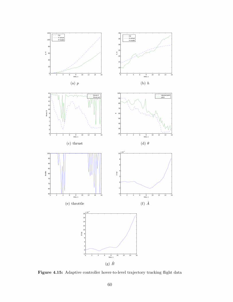
0 2 4 6 8 10 12 14 160
20
40
60
80
100
120
time, s
p, m
PdP actualP model
(a) p
0 2 4 6 8 10 12 14 165
10
15
20
25
30
35
40
time, s
h, m
HdH actualH model
(b) h
0 2 4 6 8 10 12 14 164
5
6
7
8
9
10
11
12
13
14
time, s
thru
st, N
thrust dthrust est
(c) thrust
0 2 4 6 8 10 12 14 1620
30
40
50
60
70
80
90
100
time, s
θ
desired pitchpitch
(d) θ
0 2 4 6 8 10 12 14 1660
65
70
75
80
85
90
95
100
time, s
thro
ttle
(e) throttle
0 2 4 6 8 10 12 14 16−4
−2
0
2
4
6
8
10x 10
−4
time, s
A h
at
(f) A
0 2 4 6 8 10 12 14 16−2
0
2
4
6
8
10
12
14
16
18x 10
−4
time, s
B h
at
(g) B
Figure 4.15: Adaptive controller hover-to-level trajectory tracking flight data
60
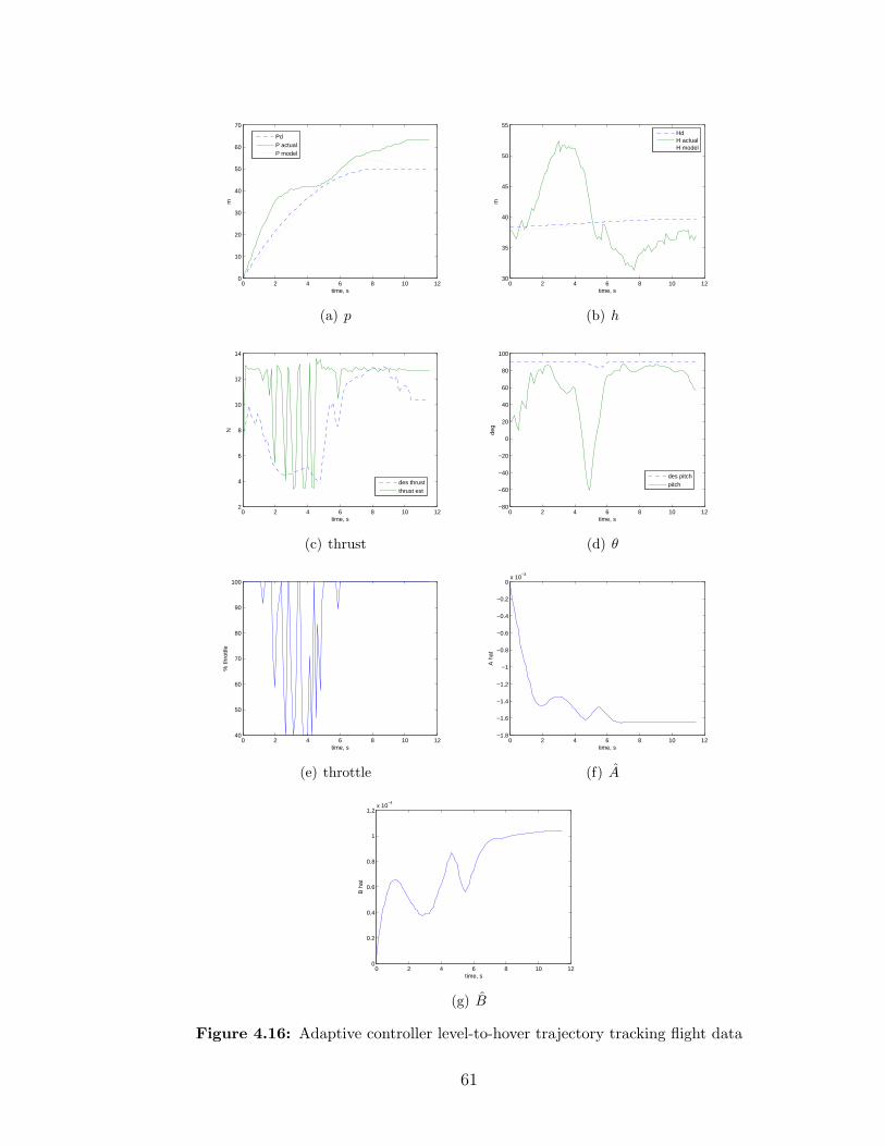
0 2 4 6 8 10 120
10
20
30
40
50
60
70
time, s
m
PdP actualP model
(a) p
0 2 4 6 8 10 1230
35
40
45
50
55
time, s
m
HdH actualH model
(b) h
0 2 4 6 8 10 122
4
6
8
10
12
14
time, s
N
des thrustthrust est
(c) thrust
0 2 4 6 8 10 12−80
−60
−40
−20
0
20
40
60
80
100
time, s
deg
des pitchpitch
(d) θ
0 2 4 6 8 10 1240
50
60
70
80
90
100
time, s
% th
rottl
e
(e) throttle
0 2 4 6 8 10 12−1.8
−1.6
−1.4
−1.2
−1
−0.8
−0.6
−0.4
−0.2
0x 10
−3
time, s
A h
at
(f) A
0 2 4 6 8 10 120
0.2
0.4
0.6
0.8
1
1.2x 10
−4
time, s
B h
at
(g) B
Figure 4.16: Adaptive controller level-to-hover trajectory tracking flight data
61
4.7 Chapter Summary
After discussing the creation of the desired trajectory generation goals and
process, three algorithms for tracking those trajectories through both types of tail-
sitter transitions were presented in this chapter. First, the simple controller was
discussed, followed by the feedback linearization controller and the adaptive con-
troller. Simulation results and flight test results were presented. In the next chapter,
the autopilot state machine will be discussed. The autopilot state machine will use
the hover position controller and level waypoint controller described in Chapter 3
along with the transition controllers presented in this chapter to fly a waypoint path
consisting of a combination of level and hover waypoints.
62
Chapter 5
Autopilot State Machine
The highest level of autopilot control code is the state machine. It contains
logic necessary to navigate a waypoint path consisting of both hover and level way-
points. The structure of the autopilot state machine is described in this chapter.
Flight results for a sample waypoint path will also be shown.
5.1 Autopilot Structure
The autopilot state machine shown in Figure 5.1 retrieves waypoints uploaded
by the Virtual Cockpit ground station and sets appropriate navigational control,
throttle, and attitude control modes to achieve desired functionality. Possible flight
commands in this autopilot are hover waypoints and level waypoints. Various flight
modes include hover flight mode, level flight mode, and modes for transitioning be-
tween these modes. The autopilot state machine code is run in an autopilot function
running at about 5 Hz. For each execution of the loop, UAV states and timers are
checked to see if a move to another state is in order. A description of each autopilot
state will be given.
It should be noted that in the autopilot state machine, hover-to-level tran-
sitions are performed immediately but level-to-hover transitions are performed only
when close enough to the desired hover waypoint. This is because of the desire to
stay in the more energy efficient level flight mode for as long as possible.
63
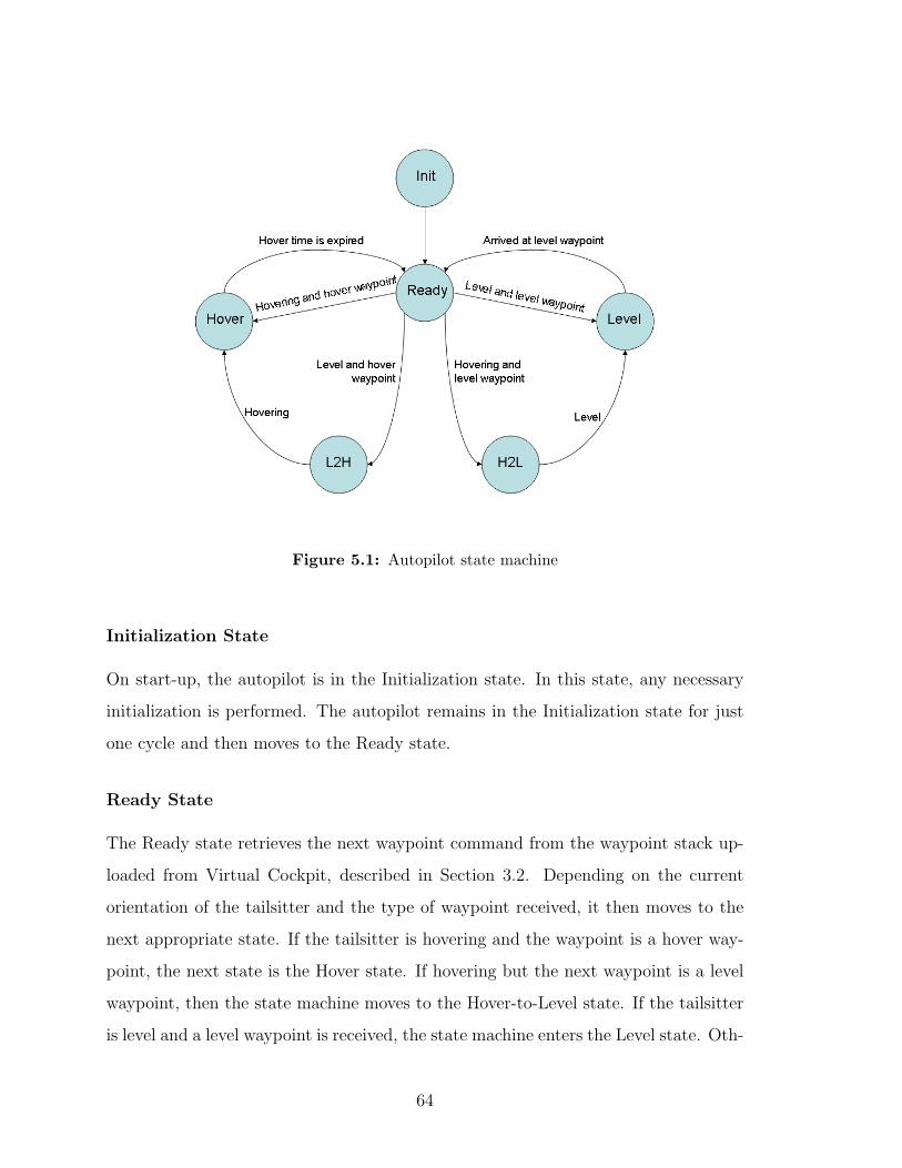
Figure 5.1: Autopilot state machine
Initialization State
On start-up, the autopilot is in the Initialization state. In this state, any necessary
initialization is performed. The autopilot remains in the Initialization state for just
one cycle and then moves to the Ready state.
Ready State
The Ready state retrieves the next waypoint command from the waypoint stack up-
loaded from Virtual Cockpit, described in Section 3.2. Depending on the current
orientation of the tailsitter and the type of waypoint received, it then moves to the
next appropriate state. If the tailsitter is hovering and the waypoint is a hover way-
point, the next state is the Hover state. If hovering but the next waypoint is a level
waypoint, then the state machine moves to the Hover-to-Level state. If the tailsitter
is level and a level waypoint is received, the state machine enters the Level state. Oth-
64
erwise, if level and the next waypoint is a hover waypoint, the Level-Level-to-Hover
state is entered.
Hover State
In this state, the hover position controller described in Section 3.4 is turned on. Also,
the throttle from altitude loop is enabled, which uses the throttle to control the
tailsitter’s altitude. When the tailsitter has arrived at the desired hover waypoint,
the state machine moves to the Maintain Hover state.
Maintain Hover State
Upon entering the Maintain Hover state a timer is initialized. Each hover waypoint
has a hover time associated with it. When this time has expired, the state machine
will move to the Ready state.
Level State
When flying between level waypoints the level flight controller described in Section 3.5
is used. Throttle is controlled along with pitch angle to maintain a desired altitude.
To control tailsitter attitude, the quaternion attitude controller is used as in the hover
flight mode, although different gains are loaded.
Rotate-to-Heading State
The Rotate to Heading state is entered before a hover to level transition is performed.
Since the transition is to be performed along a straight line, it is necessary to first
rotate the tailsitter in the direction of the new level waypoint. When the tailsitter is
within a certain angle threshold of the desired heading, the Hover to Level state is
entered.
65
Hover-to-Level State
While in the Hover-to-Level state, the desired trajectory is created and one of the
transition path following algorithms described in Chapter 4 is executed. Which algo-
rithm to perform is selectable by the user. Once the tailsitter achieves a level flight
attitude, the Level state is entered, which will take the tailsitter to its waypoint.
Level-Level-to-Hover State
This state functions just like the Level state, but will switch to the Level to Hover state
when the tailsitter arrives within a certain distance threshold of the hover waypoint.
This is to allow the tailsitter to fly in level flight mode for as long as possible to
conserve battery life.
Level-to-Hover State
The desired trajectory is created and one of the transition path following algorithms is
executed. Once the tailsitter reaches a near-hover position, the Hover state is entered.
5.2 Autopilot Flight Results with Simple Controller
Flight results are shown in Figure 5.2 for a flight path composed of two level
waypoints and two hover waypoints. The transitions in and out of the hover waypoint
are done with the simple controller described in Section 4.2. In this experiment, the
waypoints at (0,0) and (-30,-30), the first and last points of the path, are both hover
waypoints while the remaining two points are level waypoints. The autopilot state
is numbered, with the corresponding state names listed in Table 5.1. It can be seen
that the state machine successfully navigates the tailsitter in level and hover flight
modes as well as through transitions. It should be noted that the desired airspeed
has a positive value for the hover waypoints which should be corrected to read zero.
An examination of the GPS waypoint path reveals poor tracking on first in-
spection, but much of this is due to the confined flight area in which flight testing
was done. The tailsitter takes very wide turns in these results. If a larger flight test
66

area were available and longer flight path legs were flown, then the turns would not
be as noticeable and better waypoint tracking would be seen. Waypoint tracking for
the tailsitter will be much better given a long, straight level flight path rather than a
flight path with almost constant turns as is shown in the results.
The tailsitter hovers on takeoff up to its first waypoint. The tailsitter comes
within a threshold value of desired altitude at about t = 12 seconds. At that time,
the next waypoint is interpreted. Since it is a level waypoint, an immediate hover-to-
level transition is commanded, as can be seen in the plot of pitch angle. The tailsitter
switches to the level flight controller and flies to the next waypoint. During the time
the tailsitter is in level flight mode, pitch and throttle are adjusted to try to achieve
desired altitude and airspeed. At t = 50 seconds, the tailsitter is close enough to
the final hover waypoint to perform a level-to-hover transition. The tailsitter then
descends to the ground.
Table 5.1: Autopilot state machine state numbersNumber State
0 Initialization1 Ready2 Hover3 Maintain Hover4 Init Maintain Hover5 Level6 Rotate to Heading7 Hover to Level8 Init Hover to Level9 Level to Hover10 Init level to Hover11 Level-Level to Hover
67
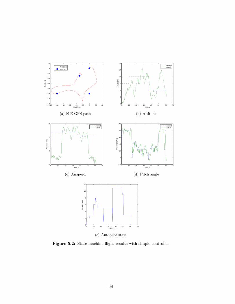
−120 −100 −80 −60 −40 −20 0 20 40−140
−120
−100
−80
−60
−40
−20
0
20
East (m)
Nor
th (
m)
measureddesired
(a) N-E GPS path
0 10 20 30 40 50 60 700
5
10
15
20
25
30
time, s
Alti
tude
(m
)
desiredactual
(b) Altitude
0 10 20 30 40 50 60 70−5
0
5
10
time, s
Airs
peed
(m
/s)
desiredactual
(c) Airspeed
0 10 20 30 40 50 60 70−20
0
20
40
60
80
100
time, s
Pitc
h an
gle
(deg
)
desiredactual
(d) Pitch angle
0 10 20 30 40 50 60 700
2
4
6
8
10
12
time, s
auto
pilo
t sta
te
(e) Autopilot state
Figure 5.2: State machine flight results with simple controller
68
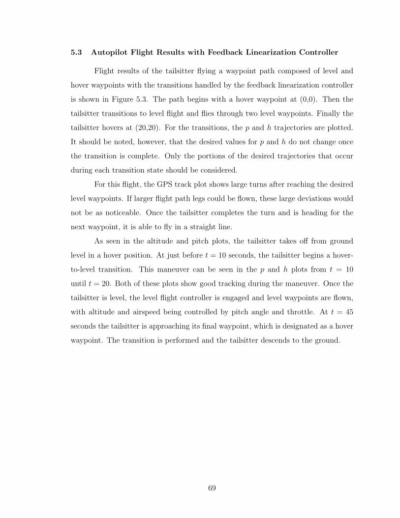
5.3 Autopilot Flight Results with Feedback Linearization Controller
Flight results of the tailsitter flying a waypoint path composed of level and
hover waypoints with the transitions handled by the feedback linearization controller
is shown in Figure 5.3. The path begins with a hover waypoint at (0,0). Then the
tailsitter transitions to level flight and flies through two level waypoints. Finally the
tailsitter hovers at (20,20). For the transitions, the p and h trajectories are plotted.
It should be noted, however, that the desired values for p and h do not change once
the transition is complete. Only the portions of the desired trajectories that occur
during each transition state should be considered.
For this flight, the GPS track plot shows large turns after reaching the desired
level waypoints. If larger flight path legs could be flown, these large deviations would
not be as noticeable. Once the tailsitter completes the turn and is heading for the
next waypoint, it is able to fly in a straight line.
As seen in the altitude and pitch plots, the tailsitter takes off from ground
level in a hover position. At just before t = 10 seconds, the tailsitter begins a hover-
to-level transition. This maneuver can be seen in the p and h plots from t = 10
until t = 20. Both of these plots show good tracking during the maneuver. Once the
tailsitter is level, the level flight controller is engaged and level waypoints are flown,
with altitude and airspeed being controlled by pitch angle and throttle. At t = 45
seconds the tailsitter is approaching its final waypoint, which is designated as a hover
waypoint. The transition is performed and the tailsitter descends to the ground.
69
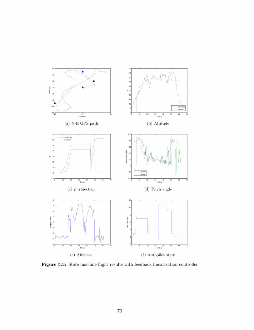
−50 0 50−80
−60
−40
−20
0
20
40
60
East (m)
Nor
th (
m)
(a) N-E GPS path
0 10 20 30 40 50 60 700
5
10
15
20
25
30
35
40
45
50
time, s
h
h desiredh actual
(b) Altitude
0 10 20 30 40 50 60 70−10
0
10
20
30
40
50
60
70
time, s
p
p desiredp actual
(c) p trajectory
0 10 20 30 40 50 60 70−40
−20
0
20
40
60
80
100
time, s
Pitc
h an
gle
(deg
)
desiredactual
(d) Pitch angle
0 10 20 30 40 50 60 70−6
−4
−2
0
2
4
6
8
10
time, s
Airs
peed
(m
/s)
(e) Airspeed
0 10 20 30 40 50 60 700
2
4
6
8
10
12
time, s
auto
pilo
t sta
te
(f) Autopilot state
Figure 5.3: State machine flight results with feedback linearization controller
70
5.4 Autopilot Flight Results with Adaptive Controller
The adaptive controller is used to negotiate transitions for the flight path
plotted in Figure 5.4. The desired flight path is the same as that used in Section 5.3,
with an initial hover waypoint followed by two level waypoints and a final hover
waypoint. Like the desired trajectories for p and h, the adaptive parameters A and
B only change during the transition state.
The GPS tracking plot looks considerably worse than the plots shown for the
simple and feedback linearization controllers. This is due to the same effects from
having short flight path legs as well as from an increase in wind during this flight.
In any case, however, the autopilot state machine as well as the adaptive controller-
managed transitions can be seen to work properly despite the poor performance of
the level and hover controllers themselves.
The tailsitter begins on the ground and hovers up to a desired altitude, where-
upon a hover-to-level transition is commanded. The pitch angle plot shows that the
transition is completed successfully, but the p plot shows that tracking in the forward
direction exhibited error of about 20 m. Tracking is off by about 10 m in the h direc-
tion during the transition, which lasts from about t = 15 seconds to t = 25 seconds.
Once in a level orientation, the level flight controller is engaged and level waypoints
are flown. At about t = 55 seconds a level-to-hover transitions is performed. Tracking
during this transition is much better in p but about the same in h.
The plots for A and B show the adaptive parameters changing during each
transition type. The values of these parameters are not changed during times when
the tailsitter is not in a transition state. These plots should only be considered for
the times when a transition is in progress. It can be seen that both parameters
approach much different values for the two different transitions, which is indicative
of the changing flight conditions when each is encountered.
71
−60 −50 −40 −30 −20 −10 0 10 20−100
−80
−60
−40
−20
0
20
40
60
80
100
East (m)
Nor
th (
m)
(a) N-E GPS path
0 10 20 30 40 50 60 70 800
10
20
30
40
50
60
time, s
h
h desiredh actual
(b) Altitude
0 10 20 30 40 50 60 70 800
5
10
15
20
25
30
35
40
45
time, s
p
p desiredp actual
(c) p trajectory
0 10 20 30 40 50 60 70 80−60
−40
−20
0
20
40
60
80
100
time, s
Pitc
h an
gle
(deg
)
desiredactual
(d) Pitch angle
0 10 20 30 40 50 60 70 80−6
−4
−2
0
2
4
6
8
10
12
time, s
Airs
peed
(m
/s)
(e) Airspeed
0 10 20 30 40 50 60 70 80−12
−10
−8
−6
−4
−2
0
2x 10
−4
time, s
A h
at
(f) A
0 10 20 30 40 50 60 70 80−4
−2
0
2
4
6
8
10x 10
−4
time, s
B h
at
(g) B
Figure 5.4: State machine flight results with adaptive controller
72

5.5 Chapter Summary
The autopilot state machine receives waypoint commands and engages appro-
priate flight modes to navigate the desired path. The state machine receives level or
hover waypoints and appropriately commands either the level flight controller, hover
position controller, or one of the transition controllers, depending on what is cur-
rently required. Flight results were given for flying a waypoint path with each of the
transition controllers described in Chapter 4.
73

74
Chapter 6
Conclusion
6.1 Summary of Results
Flight test results show the three transition trajectory tracking algorithms
working satisfactorily. The simple controller can be used in cases where a specific
trajectory does not require tracking and only a flight mode transition is desired.
When further control over the tailsitter’s path is desired, the feedback linearization
controller or adaptive controller can be used. These two controllers exhibit similar
performance, but the adaptive controller requires knowledge of fewer parameters and
therefore is the more useful of the two.
There is much room for improvement in the actual flight results. The difficul-
ties in tracking trajectories well are attributable to a number of factors. Tailsitter
position and velocity measurements are required for both feedback linearization and
adaptive controllers. Both of these measurements are obtained by GPS readings, but
these readings are subject to inaccuracies and time delays. A faster, more precise
measure of position and velocity would be needed to track the transition trajectories
well. Along with imperfect sensors, limitations in the attitude and thrust controllers
also lead to tracking error in the transition trajectory tracking algorithms. Finally,
wind of almost any strength at all is enough to disturb the tailsitter away from its
desired flight trajectory. If these limitations were addressed, the algorithms presented
in this thesis should perform much better.
6.2 Future Work
In this thesis the trajectories to track were limited to transition maneuvers
performed with the tailsitter travelling straight, with the nose/belly always facing
75
the direction of travel. However, the tailsitter is a very agile and flexible aircraft.
Tailsitter maneuverability is much greater than a fixed wing aircraft due to its ability
to hover. With a quaternion attitude representation and controller, it is theoretically
possible to command the tailsitter to any conceivable attitude. Of course, some
attitudes will be very hard to maintain for an extended period of time if they are
outside of a near hover position or in the stall region. However, future research could
focus on creating and tracking trajectories for any number of flight paths, such as
spirals, curved paths, or even aerobatic flight maneuvers.
Furthermore, each type of maneuver, like the transitions described in this
thesis or other possible maneuvers that could be developed for the tailsitter, has many
possibilities for execution. For example, a hover-to-hover maneuver with a climb
in altitude could be performed by climbing in hover mode to the correct altitude
and pitching slightly in hover mode to transition to the desired position. Or, the
same maneuver could be accomplished by transitioning to level flight, spiraling up
to the appropriate altitude, getting close to the final desired hover waypoint, and
transitioning back to hover mode. It would be a beneficial study to see what maneuver
types are more energy efficient or otherwise beneficial in different situations.
It has been suggested that the tailsitter could benefit greatly by the addition
of a downward pointing optic flow or other vision sensor. With such a sensor, hover
stabilization techniques would be possible by adjusting the control surfaces to cancel
out optic flow movements in all directions caused by wind or other factors. For
example, the tailsitter could use vision processing algorithms to identify a landing
platform and land in the proper orientation to recharge batteries. With the ability to
take-off from the ground, the tailsitter equipped with autonomous landing technology
could fly several consecutive missions without a need for human interaction.
76
Bibliography
[1] N. B. Knoebel, S. R. Osborne, J. S. Matthews, A. M. Eldredge, and R. W.Beard, “Computationally simple model reference adaptive control for miniatureair vehicles,” Proceedings of the 2006 American Control Conference, pp. 5978–5983, 2006. 3
[2] N. B. Knoebel, S. R. Osborne, D. O. Snyder, T. W. McLain, R. W. Beard,and A. M. Eldredge, “Preliminary modeling, control, and trajectory design forminiature autonomous tailsitters,” AIAA Conference on Guidance, Navigation,and Control, 2006. 3
[3] H. Stone and K. C. Wong, “Preliminary design of a tandem-wing tail-sitter UAVusing multi-disciplinary design optimisation,” International Aerospace Congress,pp. 707–720, 2004. 3
[4] H. Stone and G. Clarke, “The t-wing: A VTOL UAV for defense and civilianapplications,” UAV Australia Conference, 2001. 4
[5] R. H. Stone, “Control architecture for a tail-sitter unmanned air vehicle,” Pro-ceedings of the 5th Asian Control Conference, pp. 736–744, 2004. 4
[6] H. Stone and G. Clarke, “Optimization of transition maneuvers for a tail-sitterunmanned air vehicle (UAV),” Australian International Aerospace Congress,2001. 4
[7] http://www.aerovironment.com/. 4
[8] T. J. Cord and S. Newbern, “Unmanned air vehicles: New challenges in design,”Proceedings of the 2001 IEEE Aerospace Conference, vol. 6, pp. 2699–2704, 2001.4
[9] W. E. Green and P. Y. Oh, “A MAV that flies like an airplane and hovers like ahelicopter,” Proceedings of the 2005 IEEE/ASME International Conference onAdvanced Intelligent Mechatronics, pp. 693–698, 2005. 4
[10] ——, “A fixed-wing aircraft for hovering in caves, tunnels, and buildings,” Pro-ceedings of the 2006 American Control Conference, pp. 1092–1097, 2006. 4
[11] ——, “Autonomous hovering of a fixed-wing micro air vehicle,” Proceedings ofthe 2006 IEEE International Conference on Robotics and Automation, pp. 2164–2169, 2006. 4
77
[12] ——, “Optic flow based collision avoidance on a hybrid MAV,” IEEE Roboticsand Automation Magazine, in press. 4
[13] ——, “Flying insect inspired vision for autonomous aerial robot maneuvers innear-earth environments,” Proceedings of the 2004 IEEE International Confer-ence on Robotics and Automation, pp. 2347–2352, 2004. 4
[14] P. Y. Oh and W. E. Green, “CQAR: Closed quarter aerial robot design for recon-naissance, surveillance and target acquisition tasks in urban areas,” InternationalJournal of Computational Intelligence, vol. 1, no. 4, pp. 353–360, 2004. 4
[15] A. Ailon, “Control of a VTOL aircraft: Motion planning and trajectory track-ing,” Proceedings of the 13th Mediterranean Conference on Control and Automa-tion, pp. 1493–1498, 2005. 4
[16] P. Martin, S. Devasia, and B. Paden, “A different look at output tracking: controlof a VTOL aircraft,” Proceedings of the 33rd Conference on Decision and Control,pp. 2376–2381, 1994. 4
[17] P. Setlur, D. Dawson, Y. Fang, and B. Costic, “Nonlinear tracking control ofthe VTOL aircraft,” Proceedings of the 40th IEEE Conference on Decision andControl, pp. 4592–4597, 2001. 4
[18] B. T. Costic, D. M. Dawson, M. S. de Queiroz, and V. Kapila, “Quaternion-basedadaptive attitude tracking controller without velocity measurements,” AIAAJournal of Guidance, Control, and Dynamics, vol. 24, no. 6, pp. 1214–1222,2001. 4
[19] J. Hauser and R. Hindman, “Aggressive flight maneuvers,” Proceedings of the36th Conference on Decision and Control, pp. 4186–4191, 1997. 4
[20] M. D. Shuster, “A survey of attitude representations,” The Journal of the As-tronautical Sciences, vol. 41, no. 4, pp. 439–517, 1993. 4, 22
[21] N. B. Knoebel, Master’s Thesis. Brigham Young University, 2007. 19, 37
[22] http://www.procerusuav.com/. 20
[23] D. R. Nelson, D. B. Barber, T. W. McLain, and R. W. Beard, “Vector field pathfollowing for small unmanned air vehicles,” Proceedings of the 2006 AmericanControl Conference, pp. 5788–5794, 2006. 27
[24] H. K. Khalil, Nonlinear Systems, 3rd ed. Upper Saddle River, New Jersey:Prentice Hall, 2002. 37, 40, 44
78