TRANSIMS traﬃc ﬂow characteristics - arXiv.org e … · 2008-02-04 · PREPRINT February 4,...

arX

iv:a

dap-

org/

9710

003v

1 2

1 O

ct 1

997

TRANSIMS traffic flow characteristics

Kai Nagel†, (505) 665-0921 phone, (505) 982-0565 fax, [email protected] email

Paula Stretz†, (505) 665-6598 phone, (505) 665-7464 fax, [email protected] email

Martin Pieck†, (505) 665-0086 phone, (505) 665-7464 fax, [email protected] email

Shannon Leckey†, (505) 665-3733 phone, (505) 665-7464 fax, [email protected] email

Rick Donnelly†,∗, (505) 665-3733 phone, (505) 665-7464 fax,[email protected] email

Christopher L. Barrett† (505) 665-0430 phone, (505) 665-7464 fax, [email protected]

† Los Alamos National Laboratory, MS 997, Los Alamos NM 87545, USA

∗ Parsons Brinckerhoff, Inc., 5801 Osuna Road NE # 220, Albuquerque NM 87109, USA

PREPRINT May 30, 2018

Abstract

Knowledge of fundamental traffic flow characteristics of traffic simulation

models is an essential requirement when using these models for the planning,

design, and operation of transportation systems. In this paper we discuss the

following: a description of how features relevant to traffic flow are currently

under implementation in the TRANSIMS microsimulation, a proposition for

standardized traffic flow tests for traffic simulation models, and the results of

these tests for two different versions of the TRANSIMS microsimulation.

keywords: traffic simulation, traffic flow, intersections

0

http://arxiv.org/abs/adap-org/9710003v1

PREPRINT May 30, 2018 0


I. INTRODUCTION

One could probably reach agreement that the traffic flow behavior of traffic simulation mod-els should be well documented. Yet, in practice, this turns out to be somewhat difficult.Many traffic simulation models are under continuous development, and the traffic flow dy-namics documented in a certain publication has probably been refined and extended untilthe paper gets actually published.

It makes thus sense to agree on a certain set of tests for traffic flow dynamics which shouldalways be run and documented together with any “real” results. In this paper, we proposesuch a suite of traffic flow measurements. We are well aware of the fact that some ofthe results in this paper are arguably unrefined with respect to reality. Yet, as we statedabove, we are continuously working on improvements, and this publication represents botha snapshot of where we currently stand and an argument for a standardized traffic flowtest suite for simulation models. We hope that this publication will both open the wayfor a constructive dialogue on which standardized traffic flow tests should be run for trafficsimulation models, and which of the features of our traffic simulation models may needimprovement.

When designing a traffic microsimulation model, the first idea might be to measure all as-pects of human driving and put them in algorithmic form into the computer. Unfortunately,such attempts cause many problems. The first is a data collection problem, because onecan certainly not measure “all” aspects of human driving and is thus faced with the doublesided problem that the necessary data collection process is extremely costly and still selec-tive. Second, what if the macroscopic flow properties of such a model are clearly wrong,for example producing an hourly flow rate that is much to high or to low? Since, in such amodeling approach, one does not know the connection between the many parameters of themodel and the emergent properties (such as flow), one is left to random trial and error.

For that reason, the TRANSIMS (TRansportation ANalysis and SIMulation System [1])microsimulation starts with a minimal approach. A minimal set of driving rules is used tosimulate traffic, and this set of rules is only extended when it becomes clear that a certainimportant aspect of traffic flow behavior cannot be included with the current rule set. Besidesthe conceptual clarity, this also has the advantage that it is usually computationally fast –minimal models have few rules and thus run fast on computers. This argument also makesit clear that one wants to remain flexible with respect to refinements of the model: If certainrefinements are unnecessary with respect to a certain question, one would want to switchthem off both for conceptual clarity and for computational speed.

The questions that TRANSIMS is currently designed for are transportation planning ques-tions. The most important zeroth order result of a transportation microsimulation shouldbe the delays, since, once they occur, they dominate travel times, and also hinder dischargeof the transportation system, thus leading to grid-lock. Delays are caused by congestion,and congestion is caused by demand being higher than capacity. This implies that the firstthing the TRANSIMS traffic microsimulation has to get right are capacity constraints (andpossibly their variance). Capacity constraints are caused by a variety of effects:

• Undisturbed roadways such as freeways have capacity constraints given by the maxi-


mum of the flow-density diagram.

• Typical arterials have their capacity constraints given by traffic lights.

• In the case of unprotected turning movements (yield, stop, ramps, unprotected left,etc.), the capacity constraints are given as a function of the traffic on the “interferinglanes”. For example, the number of vehicles making an unprotected left turn dependson the oncoming traffic.

Building a simulation which can be adjusted against all these diagrams seems a hopeless taskgiven the enormous amount of degrees of freedom. The TRANSIMS approach for that reasonhas been to generate the correct behavior from a few much more basic parameters. Thecorrect behavior with respect to the above criteria can essentially be obtained by adjustingtwo parameters: (i) The value of a certain asymmetric noise parameter in the accelerationdetermines maximum flow on freeways and through traffic lights; (ii) the value of the gapacceptance determines flow for unprotected movements.

The remainder of this paper will first describe the algorithms TRANSIMS uses for the mostimportant traffic movements, and then describe the resulting flow characteristics.

II. RULES

A. Single lane uni-directional traffic

Our traffic simulation is based on a cellular automata technique, i.e., a road is composedof cells, and each cell can either be empty, or occupied by exactly one vehicle [2,3], seeFig. 1 (a). Since movement has to be from one cell to another cell, velocities have to beinteger numbers between 0 and vmax, where the unit of velocity is [cells per time-step]. Itturns out that reasonable values are [3,4]:

• length of a box = 1/ρjam = 7.5 m (ρjam = density of vehicles in a jam).

• time step = 1 sec

• maximum velocity = 5 boxes per time step = 5 · 7.5 m/sec = 135km/h ≈ 85mph

For other conditions, such as higher or lower speed limits, this can be adapted.

Note that this approach implies a coarse graining of the spatial and temporal resolution andtherefore of the velocities. A vehicle which has a speed of, say, 4 in this model stands for avehicle which has a speed anywhere between 3.5 · 7.5 meters/sec ≈ 95 km/h (59 mph) and4.49999 · 7.5 meters/sec ≈ 121 km/h (75 mph).

Vehicles move only in one direction. For an arbitrary configuration (velocity and position),one update of the traffic system consists of two steps: a velocity update step consisting ofthree consecutive rules, and a movement step according to the result of the velocity update.The whole update is performed simultaneously for all vehicles. The complete configurationat time step t is stored and the configuration at time step t+1 is computed from that “old”


information. Computationally we calculate in time step t (with the three rules) the newvelocity of each car and write this newly calculated velocity in the same site without movingthe car (velocity update). After that we move all cars according to their newly calculatedvelocity (movement update).

1. (velocity update)

For all particles i simultaneously, do the following:

IF ( vi ≥ gapi )

vi :={

gapi − 1 with probability pnoise if possible1

gapi else(close following/braking)

ELSE IF ( vi < vmax )

vi :={

vi with probability pnoisevi + 1 else

(acceleration)

ELSE (i.e. ( vi = vmax AND vi < gapi )

vi :={

vmax − 1 with probability pnoisevmax else

(free driving)

ENDIF

2. (movement update)

Move all particles i to xi(t+ 1) = xi(t) + vi.

The index i denotes the position (an integer number) of a vehicle, v(i) its current velocity,vmax its maximum speed, gap(i) the number of empty cells ahead, and pnoise is a random-ization parameter.

The first velocity rule represents noisy car following or braking. If the vehicle ahead istoo close, the vehicle itself attempts to adjusts its velocity such that it would, in the nexttime-step, reach a position just behind where the vehicle ahead is at the moment. Yet, withprobability pnoise, the vehicle is a bit slower than this.

The second velocity rule represents noisy acceleration. Essentially, the acceleration is linear(i.e. independent from current speed), but with probability pnoise, no acceleration happens inthe current time step (maybe as a result of switching gears etc.). Instead of an accelerationsequence of 0 → 1 → 2 → 3 → . . ., a possible acceleration sequence can now be 0 → 0 →

1 → 2 → 2 → 2 → 3 → . . ..

The last velocity rule represents free driving. Instead of remaining always at the samespeed, such vehicles fluctuate between vmax (with probability 1− pnoise) and vmax − 1 (withprobability pnoise). Note that a vehicle which is set to vmax−1 will go through the accelerationstep next time, thus in the next time step either staying at vmax − 1 with probability pnoiseor getting back to vmax. Note that the resulting average speed of a freely driving vehicle isthus vmax − pnoise.

This microsimulation is also fairly well understood from a theoretical perspective; see [5,6]for more information.


B. Lane changing for passing

For multi-lane traffic, the model consists of parallel single lane models with additional rulesfor lane changing. Here we describe the two lane model which can be modified to any kindof multi lane model. Lane changing is modeled by an additional update step, which is addedbefore the velocity update. The new sequence of steps is presented below. Steps two andthree are the same in the single lane model and they are executed separately for each lane.

1. Lane changing decision

2. Velocity update

3. Vehicle movement

According to this lane changing rule set the vehicles are only moving sideways during thelane changing step; forwards movement is done in the vehicle movement step. One should,though, look at the combined effect of the lane changing and the movement, and thenvehicles will usually have moved sideways and forwards. The decision to change lane isimplemented as strictly parallel update, i.e. each vehicle is making its decision based uponthe configuration at the beginning of the update.

• Lane changing decision for passing

– IF neighboring position xo(i) in other lane is vacant

∗ THEN Calculate:

· gap(i) Gap Forward in Current Lane,

· gapo(i) Gap Forward in Other Lane,

· gapb(i) Gap Backward in Other Lane,

· IF (gap(i) < v(i) AND gapo(i) > gap(i) )− THEN weight1 = 1− ELSE weight1 = 0

· weight2 = v(i)− gapf(i)

· weight3 = vmax(i)− gapb(i).

∗ IF ( weight1 > weight2 ) AND ( weight1 > weight3 )2

· THEN mark vehicle for lane change3

2Weights are used because of extensibility towards “lane changing for plan following”. See below.

3In the current version, the lane change is actually still rejected with a probability of 0.01 even

when all the rules are fulfilled. This is in order to break the following artifact or variations of

it: Assume one lane is completely occupied and one is completely empty. The above rule set will

result in these vehicles just changing back and forth between the lanes—the vehicles will never get

smeared out across the lanes. See Ref. [7] for more details.


The rules are working in the following way (see Fig. 1 (b)): First we look at the neighboringposition in the target lane. If this cell is vacant, we calculate the gap forward in the currentlane (gap), the gap forward in the target lane (gapo), and the gap backward in the target lane(gapb). With these results we calculate the weight1 to weight3 described above. Finally ifthe weight comparisons render true the car will change to the new lane. After executing thelane changing decision we calculate the new velocity for all cars and move them accordingto this velocity.

For three or more lanes, a simultaneous implementation of the lane changing decision canlead to collisions. For example, in a three-lane road two vehicles on the left and right lanecould decide to go to the same spot in the middle lane. From an algorithmic point of view,this is possible because the lane changing decision is based on the configuration on time t;but it is also an entirely realistic situation.4 To avoid collision we only allow lane changesin a certain direction in each time step:

• IF the time step is even

THEN start procedure lane changing decision to the left for cars on the middle andthen on the right lane

• IF the time step is odd

THEN start procedure lane changing decision to the right side for cars on the middleand then on the left lane

Thus, left lane changes occur only on even time steps, right lane changes occur only on oddtime steps. This behavior is collision free.

C. Lane changing for plan following

Vehicles in TRANSIMS follow route plans, i.e. they know ahead of time the sequence oflinks they intend to follow. This means that, when they approach an intersection, they needto get into the correct lanes in order to make the intended turn. For example, a vehiclewhich intends, according to its route plan, to make a left turn at the next intersection needsto get into one of the lanes which actually allow a left turn.

This is achieved in TRANSIMS by supplementing the basic lane changing rules with a biastowards the intended lanes. This bias increases with increasing urgency, i.e. with decreasingdistance to the intersection. Technically, this is achieved by adding another weight to theacceptance conditions for lane changing:

• IF (weight1 + weight4 > weight2) AND (weight1 + weight4 > weight3)

THEN change lane

4In a deeper sense, the problem is caused by the fact that the underlying decision making dynamics

has a time scale which is smaller than the time resolution of the simulation. The simulation thus

must resolve the conflict by other means.


weight4 is calculated according to

weight4 = max

[

d∗ − d

vmax

, 0

]

for lane changes in the desired direction as long as the vehicle is not in one of the correctlanes, cf. Fig. 1 (c). d is the remaining distance to the intersection, d∗ is a parameter;both are given in the unit of “cells”. d∗ is currently set to 70 cells, i.e. approx. 500 mor 1/3 of a mile, throughout the simulation. In consequence, weight4 increases from zeroto d∗/vmax = 14 during the approach to the intersection. If weight4 = 0, then it doesnot influence lane changing decision. weight4 = 1 has the same effect as a slower vehicleahead on the same lane. Further increases of weight4 more and more override the securitycriterions that the forward and the backward gap on the destination lane need to be largeenough. weight4 > vmax lets the vehicle make the lane change even if only the neighboringcell on the destination lane is free.

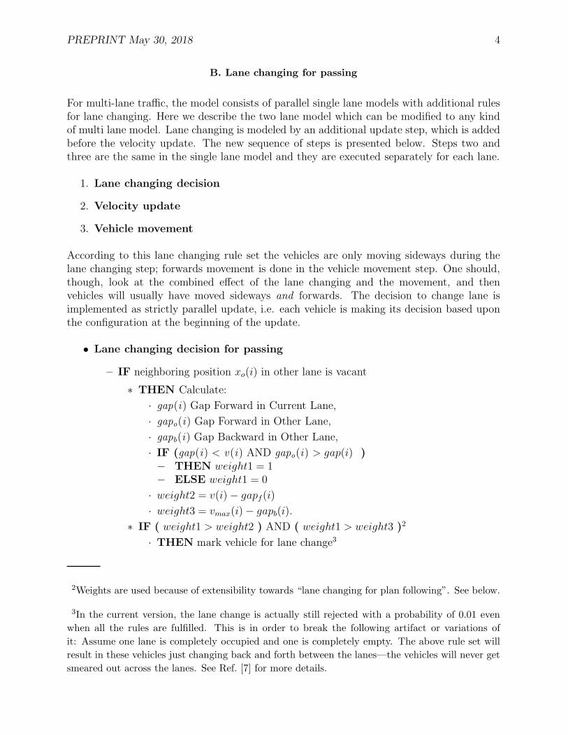
D. Unprotected turning movements

A necessary element of traffic simulations are unprotected turning movements. By this wemean that that for the movement the driver intends to make, some other lanes have priority.Examples are stop signs, yield signs, on-ramps, unprotected left turns.

The general modeling principle for this in TRANSIMS is based on a gap acceptance in theinterfering lanes, see Fig. 1 (d). Interfering lanes are the lanes which have priority; forexample, for a stop-controlled left turn onto a major road this would be all lanes comingfrom the left plus the leftmost lane coming from the right. In order to accept the turn, therehas to be a sufficient gap on each of these lanes.

Note that “gap divided by the velocity of the oncoming vehicle” is the oncoming vehicle’stime headway, which is the typical measure used in the Highway Capacity Manual [8]. Ifone wants a time headway on an interfering lane of at least 3 seconds, then a vehicle witha velocity of 4 cells/second would have to be at least 12 cells away from the intersection.

The current TRANSIMS microsimulation uses a gap acceptance (gap between intersectionand nearest car to the intersection which is approaching) of 3 times the oncoming vehicle’svelocity, i.e. when the gap on each interfering lane is larger than or equal to the first vehicleon that lane, the move is accepted. For example, if the oncoming vehicle has a speed of 3, atleast 9 empty cells have to be between the oncoming vehicle and the intersection. A specialcase is if the oncoming vehicle has the velocity zero, in which case no gap is necessary.5

5The condition for the “case study” microsimulation of TRANSIMS [9,10] was that a movement

was accepted if, for all interfering lanes, the gap was larger than vmax. That means that for fast

oncoming traffic the acceptance was higher than in the newer version, but for low speed oncoming

traffic the acceptance rate was lower—with the extreme case that no turns were possible against

oncoming traffic of speed zero.


E. Signalized intersections

In TRANSIMS, we distinguish between signalized intersections and unsignalized intersec-tions because they are modeled differently in TRANSIMS. In signalized intersections, thepriorities are changing in time and regulated by signals. In unsignalized intersections, thepriorities are fixed.

When a simulated vehicle approaches a signalized intersection, the algorithm first decides if,according to its current speed, it potentially wants to leave the link, i.e. its current speed (incells per update) is larger than or equal to the remaining number of cells on the link.6 If avehicle wants to leave the link, the algorithm checks the “traffic control”, which determinesif the vehicle can leave the link. If it encounters a red light, it can not leave the link and nofurther action is taken. If it encounters a protected (green arrow) or caution (yellow) signal,the vehicle is allowed to enter the intersection. If it encounters a permitted signal (green, forexample permitted left turn against oncoming traffic), the vehicle checks all interfering lanesfor the gap that is larger or equal to 3 times the oncoming vehicle’s velocity (see Subsec. IIDabove).

If the movement into the intersection is accepted, the vehicle is moved into an “intersectionqueue”; there is one queue for each incoming lane. This queue models vehicle behaviorinside an intersection. The vehicle gets a “time stamp”, before which it is not allowed toleave the intersection; this time stamp is representative for the duration of the movementthrough the intersection. The intersection queues have finite capacity; once they are full, nomore vehicles are accepted and the vehicles start to queue up on the link. This models thefinite vehicle storing capacity of an intersection.

Once a vehicle is ready to leave the intersection, it moves to the first cell on the destinationlink if available.7 The speed of the vehicle is not changed when it is in the intersection queueso it exits on the destination link in the first cell with the same velocity that it had when itentered the queue.

Note that vehicles turning against interfering traffic make their decision to accept the turnwhen they enter the intersection queue, not when they leave it. This can have the effectthat a vehicle enters the intersection queue when there is no oncoming traffic, but, becauseof other vehicles ahead of it in the same queue, cannot make its turn immediately. Yet, sincethe turn was already accepted, it will be executed as soon as all vehicles ahead in the samequeue have cleared the queue and a cell on the destination link is available. The turn canoccur during oncoming traffic. So in some sense vehicles will go “through” each other. Yet,note that on average the result is still correct. The approach described above will not letmore vehicles through the intersection than a gap acceptance calculated when leaving theintersection queue. The above logic was chosen for simplification purposes since unsignalizedintersections (see below) do not have queues and thus need to make their acceptance decisionswhen entering the intersection.

6Vehicles may accelerate or slow down before they actually reach the intersection. See below.

7Algorithmically, it only “reserves” a cell. See below.


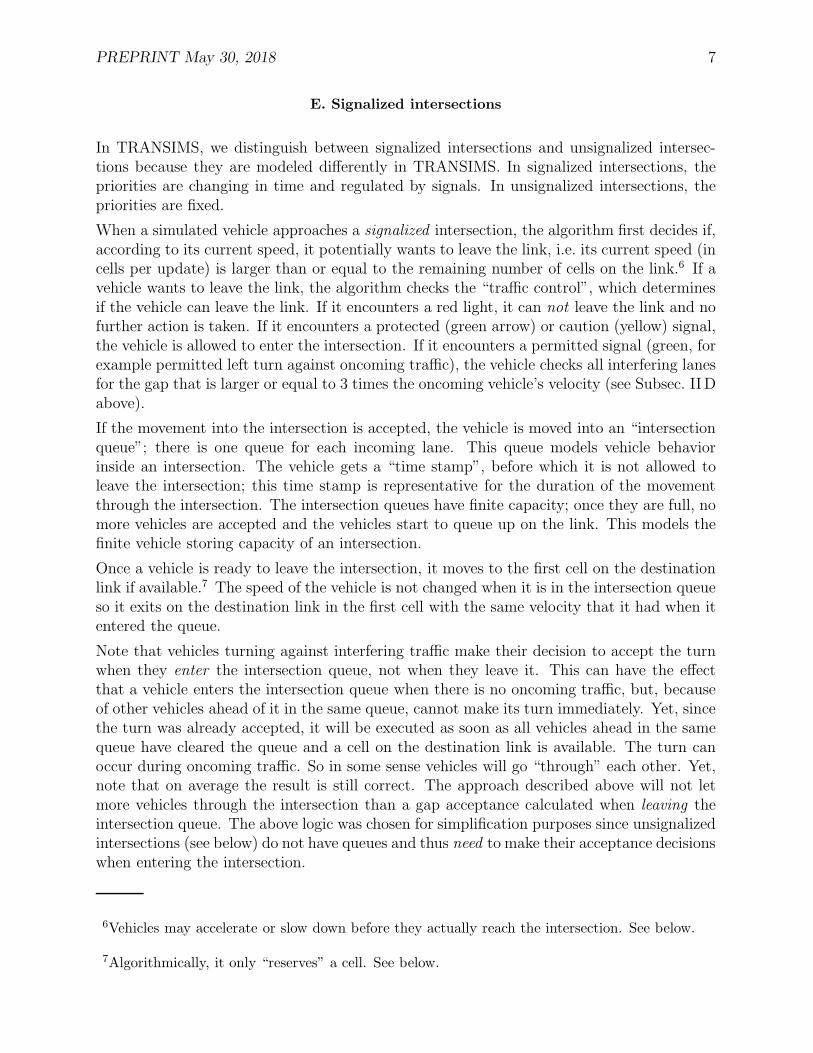
F. Unsignalized intersections

Unsignalized intersections in TRANSIMS have no internal queues, i.e. vehicles go rightthrough them.8 Also, vehicles leaving an unsignalized intersection go down the destinationlink as far as prescribed by their velocity, not just into the first cell as in the signalizedintersections. Apart from these two differences, unsignalized intersections are similar tosignalized ones.

When a simulated vehicle approaches an unsignalized intersection, the algorithm first decidesif, according to its current speed, it potentially wants to leave the link, i.e. its current speed(in cells per update) is larger than or equal to the remaining number of sites on the link. If avehicle wants to leave the link, the algorithm checks the “traffic control”, which determinesif the vehicle can leave the link. Currently occuring traffic controls are: no control, yield,and stop.

If a “no control” is encountered, the vehicle is moved to its destination cell without anyfurther checks. For example, if a vehicle has a velocity of 5 cells per update and 2 morecells to go on its link, then it attempts to go 3 cells into the destination link. If that cell isalready reserved (either by another “reservation” or by a real vehicle), then the next closercell is attempted, etc., until the algorithm either finds an empty cell or returns that thedestination lane is full. “No control” is usually used for the major directions, i.e. for thelanes which have priority.

If a “yield” is encountered, the vehicle checks the gap on all interfering lanes. According tothe same rules as above, on all interfering lanes the gap needs to be larger or equal threetimes the first vehicle’s speed on that lane. If the movement is accepted, the destination cellis selected according to the same rules as with the “no control” case.

If it encounters a “stop”, the vehicle is brought to a stop. Only when the vehicle has avelocity of zero for at least one time step on the last cell of the link, is it allowed to continue.If the result of the regular velocity update indeed accelerates the vehicle,9 then it attemptsto go through the intersection. On all interfering lanes the gap, according to the same rulesas above, needs to be larger or equal to three times the first vehicle’s speed on that lane. Ifthe movement is accepted, a vehicle coming from a stop sign will always go to the first cellon the destination link (if empty) and will have a velocity of one.

G. Parking locations

In the current TRANSIMS microsimulation, vehicular trips start and end at parking loca-tions. Each link in the microsimulation, except for freeway ramps, freeway links, and some

8Again, technically the vehicles only reserve cells on the destination links. The actual move

through the intersection happens later and can also be postponed if after the velocity update the

vehicle actually does not make it to the intersection.

9I.e. there is a probability of 1− pnoise that the vehicle will not accelerate in the given time step.


“virtual” links such as centroid connectors, has at least one parking location. Parking lo-cations thus represent the aggregated parking options on that link. Parking locations haverules about how vehicles enter and exit the simulation:

• Each vehicle in TRANSIMS has a complete route plan, together with a starting time.At the starting time, the vehicle is added to a queue of vehicles that want to leave thesame parking location. When the vehicle is the first one in the queue, it attempts toenter the link. The acceptance logic is in spirit similar to the logic of the unsignalizedintersections, i.e. vehicles check the available gap and make their decision based onthat. Parking accessory logic is not the focus of the current paper, and since that logicmay change in TRANSIMS in the near future and we also expect no influence on theresults presented here, we omit further technical details.

• A vehicle that has reached its destination parking location according to its plan willleave the microsimulation. It is simply removed from the traffic.

H. Parallel logic

TRANSIMS is designed to run on parallel computers, such as coupled workstations, desktopmulti-processors, or supercomputers. The parallelization approach used for the microsimu-lation is a geographical distribution, i.e. different geographical parts of the simulated areaare computed on different CPUs.

The current TRANSIMS microsimulation has these boundaries always in the middle of links.This is done in order to keep the complexity of the parallel computing logic as far away aspossible from the complexity of the intersection logic.

Information needs to be exchanged at the boundaries several times per update in order tokeep the dynamics consistent. For example, if a vehicle changes lanes and end up close infront of another one, that other one is probably forced to brake. Now, if the lane changingvehicle is on one CPU and the following one on another, one needs to communicate the lanechange. This will be called “Update boundaries” in the following section.

I. Complete scheduling

For a complete transportation microsimulation, we need to specify when movements are ac-cepted, and also how conflicts are resolved. For example, vehicles simultaneously attemptingto change lanes into the middle lane represent such a conflict. Another conflict is two vehiclesfrom two different links competing for the same site on the destination link.

The complete update of the current TRANSIMS microsimulation is as follows. Assume thatthe state at time t is the result of the last update. Let t1, t2, etc. be intermediate partialtime steps.

1. Vehicles which are ready to leave intersection queues from signalized intersectionsreserve cells on outgoing lanes. They only attempt to reserve the first cell on the link;


their velocity is the same as it was when they entered the intersection. When the cellis occupied (either by another “reservation” or by a vehicle), then the vehicle cannotleave the intersection. Note that there can be a conflict between different queues forthe same destination cell. The current solution in TRANSIMS is that queues areserved on a first come first served basis in some arbitrarily defined way, i.e. a queuewhich happens to be treated earlier in the microsimulation has a slightly higher chanceof unloading its vehicles. — Result: t1 information.

2. Vehicles change Lanes. Use information from time t1 to calculate situation at time t2.

3. Exit from Parking. Results in t3 information.

4. Exchange boundary information for parallel computing.

5. Non-signalized intersections reserve sites on target lanes. Note that there can be aconflict of two incoming links competing for the same destination cell. The currentsolution in TRANSIMS is that links are served on a first come first served basis,i.e. a link which happens to be treated earlier in the microsimulation has a slightlyhigher chance of unloading its vehicles. Note that this conflict only happens betweenminor links. Major links never compete for the same outgoing link except when thereis a network coding error; and for the competition between major and minor links,the major link always wins because of the interfering lanes conditions.10 Result: t4information.

6. Calculate speeds and do movements. If a vehicle scheduled for an intersection doesnot go through the intersection as a result of the velocity update, the reservation iscancelled. Vehicles which go through unsignalized intersections have p set to zero,i.e. if it turns out that the result of the velocity update indeed brings them into theintersection, they need to go to the site on the destination lane which was reservedearlier. Result: t5 = t+ 1 information.

7. Exchange boundary information and migrate vehicles for parallel computing.

III. STANDARDIZED FLOW TEST SUITE FOR SIMULATION MODELS

In order to control the effect of driving rules, TRANSIMS provides controlled tests for trafficflow behavior. These tests are simplified situations where elements of the microsimulationcan be tested in isolation. This test suite uses the standard microsimulation code in the sameway it is used for full-scale regional simulations, and it also uses the same input and outputfacilities: The test network is currently defined via a table in an oracle data base, in the sameformat as the Dallas/Fort Worth network is kept. Input of vehicles is, following individualvehicle’s plans, via parking locations, the same way vehicles enter regional simulations.

10Note that the situation slightly different when the speed of the vehicle on the major link is

zero—see below.


Output is collected on certain parts of the network on a second-by-second basis, the sameway it can be collected for regional microsimulations. The collected output is then post-processed to obtain the aggregated results presented in this paper.

The test cases we look at in this paper are the following (see also Fig. 1 (e)):

• One-lane traffic, in order to see if car following behavior generates reasonable funda-mental diagrams.

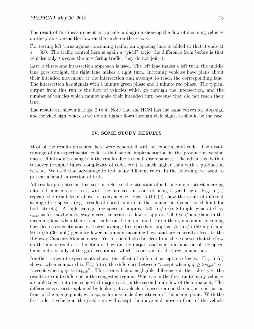
• Three-lane traffic, in order to see if the addition of passing lane changing behavior stillgenerates reasonable fundamental diagrams, and in order to look at lane usage.

• Stop sign, yield sign, and left turns against oncoming traffic, in order to see it the logicfor non-signalized intersections generates acceptable flow rates.

• A signalized intersection, in order to see of we obtain reasonable flow rates, and inorder to check lane changing behavior for plan following purposes.

A. Measured quantities

We look at three minute averages of the following quantities:

• Local Flow. Flow q is defined as usual by:

q =N

T[vehicles/hour]

N is the number of cars which pass a certain site at a time period T .

• Local Density. Density is in principle easily defined, ρ = N/L, where N is thenumber of vehicles on a piece of roadway of length L. Yet, given current sensoringtechnology, this is not easy to achieve since one would need a sensor which counts,say once a second, cars on a predefined stretch of length L of the roadway. For thatreason, empirical papers sometimes resort to occupancy, which is the fraction of timea given sensor has been occupied by a vehicle. Current TRANSIMS measures densityaccording to its original definition, i.e., once a time step, we count the number ofvehicles on a stretch of roadway of L = 5 sites = 5× 7.5 m = 37.5 m.11 We add thesecounts for k = 180 measurement events and then divide the resulting number by Land by k:

ρ =N

k ∗ L

11The “magical” number of L = 5 sites is equal to the maximum velocity of vmax = 5 sites/update.

This ensures that each vehicle is counted at least once.


The result can be scaled to convenient units, for example “vehicles per km”.

Note that this way of computing density averages the counts over a length of 37.5 m,which is longer than the usual sensor extensions. The effect of this should be system-atically studied.

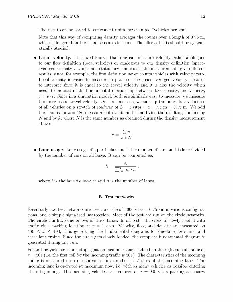
• Local velocity. It is well known that one can measure velocity either analogousto our flow definition (local velocity) or analogous to our density definition (space-averaged velocity). Under non-stationary conditions, the measurements give differentresults, since, for example, the first definition never counts vehicles with velocity zero.Local velocity is easier to measure in practice; the space-averaged velocity is easierto interpret since it is equal to the travel velocity and it is also the velocity whichneeds to be used in the fundamental relationship between flow, density, and velocity,q = ρ · v. Since in a simulation model, both are similarly easy to measure, we measurethe more useful travel velocity. Once a time step, we sum up the individual velocitiesof all vehicles on a stretch of roadway of L = 5 sites = 5 × 7.5 m = 37.5 m. We addthese sums for k = 180 measurement events and then divide the resulting number byN and by k, where N is the same number as obtained during the density measurementabove:

v =

∑

v

k ∗N

• Lane usage. Lane usage of a particular lane is the number of cars on this lane dividedby the number of cars on all lanes. It can be computed as:

fi =ρi

∑nj=1

ρj · n,

where i is the lane we look at and n is the number of lanes.

B. Test networks

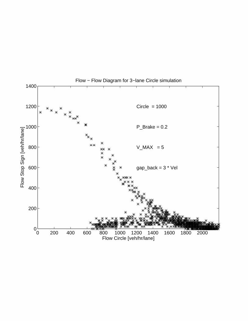
Essentially two test networks are used: a circle of 1 000 sites = 0.75 km in various configura-tions, and a simple signalized intersection. Most of the test are run on the circle networks.The circle can have one or two or three lanes. In all tests, the circle is slowly loaded withtraffic via a parking location at x = 1 sites. Velocity, flow, and density are measured on486 ≤ x ≤ 490, thus generating the fundamental diagrams for one-lane, two-lane, andthree-lane traffic. Since the circle gets slowly loaded, the complete fundamental diagram isgenerated during one run.

For testing yield signs and stop signs, an incoming lane is added on the right side of traffic atx = 501 (i.e. the first cell for the incoming traffic is 501). The characteristics of the incomingtraffic is measured on a measurement box on the last 5 sites of the incoming lane. Theincoming lane is operated at maximum flow, i.e. with as many vehicles as possible enteringat its beginning. The incoming vehicles are removed at x = 900 via a parking accessory.


The result of this measurement is typically a diagram showing the flow of incoming vehicleson the y-axis versus the flow on the circle on the x-axis.

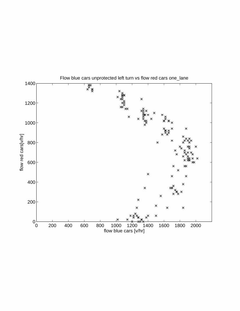
For testing left turns against oncoming traffic, an opposing lane is added so that it ends atx = 500. The traffic control here is again a “yield” logic; the difference from before is thatvehicles only traverse the interfering traffic, they do not join it.

Last, a three-lane intersection approach is used. The left lane makes a left turn, the middlelane goes straight, the right lane makes a right turn. Incoming vehicles have plans abouttheir intended movement at the intersection and attempt to reach the corresponding lane.The intersection has signals with 1 minute green phase and 1 minute red phase. The typicaloutput from this run is the flow of vehicles which go through the intersection, and thenumber of vehicles which cannot make their intended turn because they did not reach theirlane.

The results are shown in Figs. 2 to 4. Note that the HCM has the same curves for stop signand for yield sign, whereas we obtain higher flows through yield signs, as should be the case.

IV. SOME STUDY RESULTS

Most of the results presented here were generated with an experimental code. The disad-vantage of an experimental code is that actual implementation in the production versionmay still introduce changes in the results due to small discrepancies. The advantage is thatturnover (compile times, complexity of code, etc.) is much higher than with a productionversion. We used that advantage to test many different rules. In the following, we want topresent a small subsection of tests.

All results presented in this section refer to the situation of a 1-lane minor street merginginto a 1-lane major street, with the intersection control being a yield sign. Fig. 5 (a)repeats the result from above for convenience. Figs. 5 (b)–(c) show the result of differentaverage free speeds (e.g. result of speed limits) in the simulation (same speed limit forboth streets). A high average free speed of approx. 130 km/h (≈ 80 mph, generated byvmax = 5), maybe a freeway merge, generates a flow of approx. 2000 veh/hour/lane in theincoming lane when there is no traffic on the major road. From there, maximum incomingflow decreases continuously. Lower average free speeds of approx. 75 km/h (50 mph) and50 km/h (30 mph) generate lower maximum incoming flows and are generally closer to theHighway Capacity Manual curve. Yet, it should also be clear from these curves that the flowon the minor road as a function of flow on the major road is also a function of the speedlimit and not only of the gap acceptance, which is constant in all three simulations.

Another series of experiments shows the effect of different acceptance logics. Fig. 5 (d)shows, when compared to Fig. 5 (a), the difference between “accept when gap ≥ 3vback” vs.“accept when gap > 3vback”. This seems like a negligible difference in the rules; yet, theresults are quite different in the congested regime. Whereas in the first, quite many vehiclesare able to get into the congested major road, in the second, only few of them make it. Thedifference is easiest explained by looking at a vehicle of speed zero on the major road just infront of the merge point, with space for a vehicle downstream of the merge point. With thefirst rule, a vehicle at the yield sign will accept the move and move in front of the vehicle


on the major road, in the second case, it will not. Both scenarios seem to be plausible tous; only systematic measurements can probably resolve which one is better for a simulationmodel.

A last series of experiments shows the effect of different values for the gap acceptance.Figs. 5 (e) and (f) show “accept when gap > vback and gap > vmax. Clearly, more vehiclesare accepted, leading to a higher flow of turning vehicles as a function of the flow on themajor road. Note that the flow via the yield sign is never higher than 1800 minus the flowon the major road. This reflects the fact that the major road cannot have a higher flowthan 1800 veh/h/lane (free speed approx 50 mph); traffic through the yield sign can thus atmost fill the major road to capacity. This explains why the much weaker gap acceptances tonot produce even more difference in the regime where the major road is uncongested. Thesituation is clearly different for unprotected turns across instead of into traffic, as can beseen for the left turns in the next section.

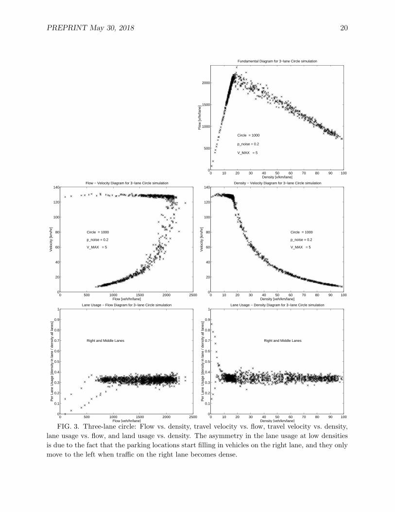
V. COMPARISON TO CASE STUDY LOGIC

The gap acceptance logic presented here and used in the current TRANSIMS microsimula-tion is different from the logic used in the “Dallas/Fort Worth Case Study” [9,10]. The logicduring that case study was: “Accept an unprotected movement if in all interfering lanes thegap is larger than vmax = 5.” This means that at low flow rates on the major road, moreturns were accepted, whereas at high flow rates on the major road, less turns were accepted.

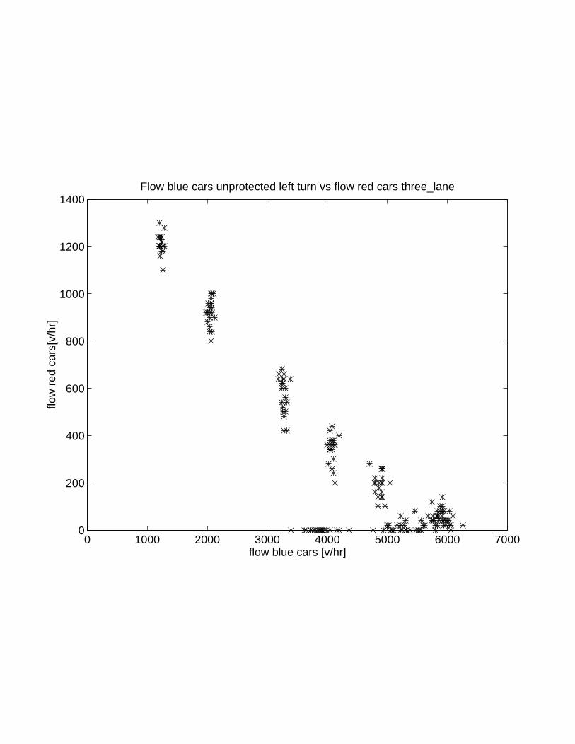
Fig. 6 compares the results for the current gap-acceptance logic and the one used in the casestudy for the case where the major road is a 3-lane road. Note that the results for the turnsinto other traffic are not that much different whereas the result for the turns across othertraffic yields dramatically higher flows with the case study logic. This is due to the fact thatfor turns into other traffic, there is a capacity constraint of the form that the joint flowsfrom the major and the incoming road cannot exceed capacity of the major road. Such aconstraint obviously does not exist for turns across the major road.

VI. SUMMARY AND CONCLUSION

In transportation simulation models for larger scale questions such as planning, the flowcharacteristics of the traffic dynamics are in some sense more important than the microscopicdriving dynamics of the vehicles itself. This becomes especially true since a “complete”representation of human driving is impossible anyway, both due to knowledge constraintsand due to computational constraints. Yet, calibrating a traffic simulation model againstall types of desired behavior (for example against all HCM curves and values mentioned inthis paper) seems a hopeless task given the high degrees of freedom.

TRANSIMS thus attempts to generate plausible macroscopic behavior from simplified mi-croscopic rules. This paper described the more important aspects of these rules as currentlyimplemented or under implementation in TRANSIMS. Before we implement rules in theTRANSIMS production version, we usually try to run systematic studies with more exper-


imental versions. The results of the traffic flow behavior from that study were presented.Also, we showed the effects of some changes in the rules for the example of a yield sign.Finally, some comparisons were made between the logic currently under implementation andthe logic used for the Dallas/Fort Worth case study.

One problem with microscopic approaches is that, in spite of all possible diligence, subtledifferences between design and actual implementation can make a significant difference inthe macroscopic outcome. For that reason, this paper should also be seen as an argumentfor a standardized traffic flow test suite for simulation models. We propose that simulationmodels, when used for studies, should first run these tests to see how the macroscopic flowdynamics actually is. We think that the combination of results presented in Figs. 2 to 4are a good test set, although extensions may be necessary in the future (e.g. merge lanes,weaving, etc.). We will attempt to provide future TRANSIMS results also with updatedversions of the results of the traffic flow tests.


REFERENCES

[1] TRANSIMS, TRansportation ANalysis and SIMulation System, Los Alamos NationalLaboratory, Los Alamos, U.S.A. See http://www-transims.tsasa.lanl.gov.

[2] Kai Nagel. Freeway traffic, cellular automata, and some (self-organizing) criticality.In R.A. de Groot and J. Nadrchal, editors, Physics Computing ’92, page 419. WorldScientific, 1993.

[3] K. Nagel and M. Schreckenberg. A cellular automaton model for freeway traffic. J. Phys.I France, 2:2221, 1992.

[4] C.L. Barrett, S. Eubank, K. Nagel, J. Riordan, and M. Wolinsky. Issues in the repre-sentation of traffic using multi-resolution cellular automata. Los Alamos UnclassifiedReport 95-2658, Los Alamos National Laboratory, 1995.

[5] K. Nagel. Particle hopping models and traffic flow theory. Phys. Rev. E, 53(5):4655,1996.

[6] K. Nagel. Fluid-dynamical vs. particle hopping models for traffic flow. In D.E.Wolf,M.Schreckenberg, and A.Bachem, editors, Traffic and granular flow, page 41. WorldScientific, Singapore, 1996.

[7] M. Rickert, K. Nagel, M. Schreckenberg, and A. Latour. Two lane traffic simulationsusing cellular automata. Physica A, 231:534, 1996.

[8] Transportation Research Board. Highway Capacity Manual. Special Report No. 209.National Research Council, Washington, D.C., 3rd edition, 1994.

[9] R.J. Beckman et al. TRANSIMS Dallas/Fort Worth case study report. Technical report,Los Alamos National Laboratory, TSA-Division, Los Alamos, NM 87545, 1997. To bereleased.

[10] K. Nagel and C.L.Barrett. Using microsimulation feedback for trip adaptation for real-istic traffic in Dallas. International Journal of Modern Physics C, 8(3):505–526, 1997.


FIGURES

1 5 2

gap

1 vehicle with velocity 1 cell per time-step (a)

5

3 2

2

forward gapbackward gap

gap

forward gap

gap

Situation I

Situation II

5

2

3

backward gap

(b)

Wrong Lane

Turn Lane

Weight 4

1212120 1 1 1 1 1 2 131312 13 13 13 14

No Weight 4 added for lane changing

4

3

Weight 4 added for lane changing (c) 1

5

3

5

3

2

1

2

3

gap = 3 * velocity(oncoming vehicle) (d)

Locationx=1

Flow

ParkingLane

Box

Opposing Lane

Measurement

Incoming

ParkingAccessory

x=501x=490x=486

x=900

(e)


FIG. 1. (a) Definition of gap and examples for one-lane update rules. Traffic is moving to the

right. The leftmost vehicle accelerates to velocity 2 with probability 0.8 and stays at velocity 1 with

probability 0.2. The middle vehicle slows down to velocity 1 with probability 0.8 and to velocity 0

with probability 0.2. The right most vehicle accelerates to velocity 3 with probability 0.8 and

stays at velocity 2 with probability 0.2. Velocities are in “cells per time step”. All vehicles are

moved according to their velocities at a later phase of the update. (b) Illustration of lane changing

rules. Traffic is moving to the right; only lane changes to the left are considered. Situation I: The

leftmost vehicle on the bottom lane will change to the left because (i) the forward gap on its own

lane, 1, is smaller than its velocity, 3; (ii) the forward gap in the other lane, 10, is larger than

the gap on its own lane, 1; (iii) the forward gap is large enough compared to its own velocity:

weight2 = v − gapf = 3 − 10 = −7 < 1 = weight1; (iv) the backward gap is large enough:

weight3 = vmax − gapb = 5 − 6 = −1 < 1 = weight1. Situation II: The second vehicle from the

right on the right lane will not accept a lane change because the gap backwards on the target lane

is not sufficient. (c) Value of weight4 when in wrong lane during the approach to the intersection.

(d) Example of a left turn against oncoming traffic. The turn is accepted because on all three

oncoming lanes, the gap is larger or equal to three times the first oncoming vehicle’s velocity. (e)

Test networks.


0 10 20 30 40 50 60 70 80 90 1000

500

1000

1500

2000

Density [v/km/lane]

Flo

w [v

/hr/

lane

]

Fundamental Diagram for 1−lane Circle simulation

Circle = 1000

p_noise = 0.2

V_MAX = 5

0 500 1000 1500 2000 25000

20

40

60

80

100

120

140

Flow [veh/hr/lane]

Vel

ocity

[km

/hr]

Flow − Velocity Diagram for 1−lane Circle simulation

Circle = 1000

p_noise = 0.2

V_MAX = 5

0 10 20 30 40 50 60 70 80 90 1000

20

40

60

80

100

120

140

Density [veh/km/lane]

Vel

ocity

[km

/hr]

Density − Velocity Diagram for 1−lane Circle simulation

Circle = 1000

p_noise = 0.2

V_MAX = 5

(a)

0 5 10 15 20 25800

850

900

950

1000

1050

1100

1150

1200

Flo

w T

−In

ters

ectio

n [v

eh/h

r/la

ne]

Time [min]

Time − Flow Diagram for traffic light controlled T−intersection

(b)FIG. 2. (a) One-lane traffic: Flow vs. density, travel velocity vs. flow, and travel velocity vs.

density. (b) Number of vehicles going through the intersection and number of vehicles “off plan”

per green phase, re-scaled to hourly flow rates per lane.


0 10 20 30 40 50 60 70 80 90 1000

500

1000

1500

2000

Density [v/km/lane]

Flo

w [v

/hr/

lane

]


Circle = 1000

p_noise = 0.2

V_MAX = 5

0 500 1000 1500 2000 25000

20

40

60

80

100

120

140

Flow [veh/hr/lane]

Vel

ocity

[km

/hr]

Flow − Velocity Diagram for 3−lane Circle simulation

Circle = 1000

p_noise = 0.2

V_MAX = 5

0 10 20 30 40 50 60 70 80 90 1000

20

40

60

80

100

120

140


Vel

ocity

[km

/hr]

Density − Velocity Diagram for 3−lane Circle simulation

Circle = 1000

p_noise = 0.2

V_MAX = 5

0 500 1000 1500 2000 25000

0.1

0.2

0.3

0.4

0.5

0.6

0.7

0.8

0.9

1

Flow [veh/hr/lane]

Per

Lan

e U

sage

[den

sity

in la

ne /

dens

ity a

ll la

nes]

Lane Usage − Flow Diagram for 3−lane Circle simulation

Right and Middle Lanes

0 10 20 30 40 50 60 70 80 90 1000

0.1

0.2

0.3

0.4

0.5

0.6

0.7

0.8

0.9

1


Per

Lan

e U

sage

[den

sity

in la

ne /

dens

ity a

ll la

nes]

Lane Usage − Density Diagram for 3−lane Circle simulation

Right and Middle Lanes

FIG. 3. Three-lane circle: Flow vs. density, travel velocity vs. flow, travel velocity vs. density,

lane usage vs. flow, and land usage vs. density. The asymmetry in the lane usage at low densities

is due to the fact that the parking locations start filling in vehicles on the right lane, and they only

move to the left when traffic on the right lane becomes dense.


0 200 400 600 800 1000 1200 1400 1600 1800 20000

200

400

600

800

1000

1200

1400

Flow Circle [veh/hr/lane]

Flo

w S

top

Sig

n [v

eh/h

r/la

ne]

Flow − Flow Diagram for 1−lane Circle simulation

Circle = 1000

p_noise = 0.2

V_MAX = 3

gap_back = 3 * Vel

−−− HCM

0 200 400 600 800 1000 1200 1400 1600 1800 20000

200

400

600

800

1000

1200

1400


Flo

w S

top

Sig

n [v

eh/h

r/la

ne]


Circle = 1000

p_noise = 0.2

V_MAX = 3

gap_back = 3 * Vel

−−− HCM

0 200 400 600 800 1000 1200 1400 1600 1800 20000

200

400

600

800

1000

1200

1400

1600

1800

2000


Flo

w Y

ield

Sig

n [v

eh/h

r/la

ne]


Circle = 1000

p_noise = 0.2

V_MAX = 3

gap_back = 3 * Vel

−−− HCM

0 200 400 600 800 1000 1200 1400 1600 1800 20000

200

400

600

800

1000

1200

1400

1600

1800

2000


Flo

w Y

ield

Sig

n [v

eh/h

r/la

ne]


Circle = 1000

p_noise = 0.2

V_MAX = 3

gap_back = 3 * Vel

−−− HCM

0 200 400 600 800 1000 1200 1400 1600 1800 20000

200

400

600

800

1000

1200

1400

1600

1800

2000


Flo

w L

eft T

urn

[veh

/hr/

lane

]


Circle = 1000

p_noise = 0.2

V_MAX = 3

gap_back = 3 * Vel

−− HCM

0 200 400 600 800 1000 1200 1400 1600 1800 20000

200

400

600

800

1000

1200

1400

1600

1800

2000


Flo

w L

eft T

urn

[veh

/hr/

lane

]


Circle = 1000

p_noise = 0.2

V_MAX = 3

gap_back = 3 * Vel

−− HCM

FIG. 4. Flow through stop sign, yield sign, and unprotected left turn. Left column: one-lane

traffic on major road (circle). Right column: two-lane traffic on major road (circle). Solid line:

Highway Capacity Manual [8]. Note that for “left turn across two lanes” (bottom right) the

interfering volume is the sum of both lanes, i.e. twice the value show on the x-axis.


0 200 400 600 800 1000 1200 1400 1600 1800 20000

200

400

600

800

1000

1200

1400

1600

1800

2000


Flo

w Y

ield

Sig

n [v

eh/h

r/la

ne]


Circle = 1000

p_noise = 0.2

V_MAX = 3

gap_back > 3 * Vel

−−− HCM

0 200 400 600 800 1000 1200 1400 1600 1800 20000

200

400

600

800

1000

1200

1400

1600

1800

2000


Flo

w Y

ield

Sig

n [v

eh/h

r/la

ne]


Circle = 1000

p_noise = 0.2

V_MAX = 5

gap_back > 3 * Vel

0 200 400 600 800 1000 1200 1400 1600 1800 20000

200

400

600

800

1000

1200

1400

1600

1800

2000


Flo

w Y

ield

Sig

n [v

eh/h

r/la

ne]


Circle = 1000

p_noise = 0.2

V_MAX = 2

gap_back > 3 * Vel

0 200 400 600 800 1000 1200 1400 1600 1800 20000

200

400

600

800

1000

1200

1400

1600

1800

2000


Flo

w Y

ield

Sig

n [v

eh/h

r/la

ne]


Circle = 1000

p_noise = 0.2

V_MAX = 3

gap_back >= 3 * Vel

0 200 400 600 800 1000 1200 1400 1600 1800 20000

200

400

600

800

1000

1200

1400

1600

1800

2000


Flo

w Y

ield

Sig

n [v

eh/h

r/la

ne]


Circle = 1000

p_noise = 0.2

V_MAX = 3

gap_back > Vel

0 200 400 600 800 1000 1200 1400 1600 1800 20000

200

400

600

800

1000

1200

1400

1600

1800

2000


Flo

w Y

ield

Sig

n [v

eh/h

r/la

ne]


Circle = 1000

p_noise = 0.2

V_MAX = 3

gap_back > V_MAX

FIG. 5. Comparison between different rules for the case of a 1-lane minor road controlled by a

yield sign merging into a 1-lane major road. (a) Figure as shown earlier, i.e. “accept if gap > 3vback”

and vmax = 3. (b) – (c) Effect of different maximum velocities vmax = 5 and vmax = 2. (d) Effect

of a slightly different acceptance rule “accept if gap ≥ 3vback” (vmax = 3). (e) – (f) Effect of

weaker gap acceptances “accept if gap > vback” and “accept if gap > vmax” (vmax = 3).


1000 1200 1400 1600 1800 2000 2200 24000

100

200

300

400

500

600


Flo

w S

top

Sig

n [v

eh/h

r/la

ne]


Circle = 1000

p_noise = 0.2

V_MAX = 5

gap_back = 3 * Vel

1000 1200 1400 1600 1800 2000 2200 24000

100

200

300

400

500

600


Flo

w S

top

Sig

n [v

eh/h

r/la

ne]

Flow − Flow Diagram (TRANSIMS) for 3−lane Circle simulation

1000 1200 1400 1600 1800 2000 2200 24000

100

200

300

400

500

600

700

800


Flo

w Y

ield

Sig

n [v

eh/h

r/la

ne]


Circle = 1000

p_noise = 0.2

V_MAX = 5

gap_back = 3 * Vel

1000 1200 1400 1600 1800 2000 2200 24000

100

200

300

400

500

600

700

800


Flo

w Y

ield

Sig

n [v

eh/h

r/la

ne]


1000 1200 1400 1600 1800 2000 2200 24000

100

200

300

400

500

600

700

800


Flo

w L

eft T

urn

[veh

/hr/

lane

]


Circle = 1000

p_noise = 0.2

V_MAX = 5

gap_back = 3 * Vel

1000 1200 1400 1600 1800 2000 2200 24000

100

200

300

400

500

600

700

800


Flo

w L

eft T

urn

[veh

/hr/

lane

]


FIG. 6. Comparison between current TRANSIMS microsimulation gap acceptance logic and

the one used in the case study where the major road has three lanes. Flow through stop sign, yield

sign, and unprotected left turn into/across one-lane traffic on major road. Left column: current

TRANSIMS microsimulation. Right column: case study TRANSIMS microsimulation. Note that

the results for the turns into other traffic are not that much different whereas the result for the

turns across other traffic yields much higher flows with the case study logic.

L o s A l a m o s N a t i o n a l L a b o r a t o r y

505-665-6598FAX 505-665-2083

14 of 14

Movement

v=4v=2 v=3Before

After v=2 v=2 v=5

Rules:

If gap > speed, speed = speed + 1. If gap < speed, speed = gap. (No collisions) Sometimes slow down for no reason.


505-665-6598FAX 505-665-2083

13 of 14

Left Lane Change

v=3

Gap = 3Gap Forward = 5Gap Backward = 5Desired Speed = 4Current Speed = 3

Weight1 = 4 > 3 AND 5 > 3 = 1Weight2 = 3 - 5 = -2Weight3 = 5 - 5 = 0

Lane Change = (1 > -2) AND (1 > 0) = 1


505-665-6598FAX 505-665-2083

12 of 14

Stop-After Movement

v=1Link 3 Link 2

Link 1

v=2

v=5v=4

v=3 v=5 v=2


505-665-6598FAX 505-665-2083

11 of 14

Stop--Before Movement

v=0

Link 3 Link 2

Link 1v=3

v=5v=5

v=3 v=5 v=3


505-665-6598FAX 505-665-2083

10 of 14

Link 4

Link 1

Link 2

Link 3


505-665-6598FAX 505-665-2083

9 of 14

Signal - Phase 2

Link 3 Link 2

Link 1


505-665-6598FAX 505-665-2083

8 of 14

Signal - Phase 1

Link 3 Link 2

Link 1


505-665-6598FAX 505-665-2083

7 of 14

Rules for Traffic Signal

Protected, Caution (green, yellow): Proceed if intersection buffer not full.

Wait (red): Move as far as possible on current link, (gap > 0), then wait.

Permitted: Proceed if gap on interfering lanes >= maxV, intersection buffer not full.


505-665-6598FAX 505-665-2083

6 of 14

Rules for Yield

Proceed if:

Gap on interfering lanes >= maxV.

Destination cell on destination link vacant.


505-665-6598FAX 505-665-2083

5 of 14

Rules for Stop

Proceed if:

Stopped for at least 1 time step.

Gap on interfering lanes >= maxV.

Destination cell on destination link vacant.


505-665-6598FAX 505-665-2083

4 of 14

Plan Following Rules

Lane Changes to follow plan ignored until vehicle is within theconsideration distance (70 cells from intersection).

Is current lane an acceptable lane for plan following?

Yes - bias vehicle to stay in current lane (Weight 4 = -1).

No - bias vehicle to change lanes based on distance fromintersection. (Weight 4 = MaxSpeed - (Distance FromIntersection - MaxSpeed) / 13)

Execute lane change rules modified to include plan followingweight (Weight 4).

Weight 1 = (Gap in current lane < desired speed AND GapForward in new lane > Gap in current lane) + Weight4.


505-665-6598FAX 505-665-2083

3 of 14

Lane Change Rules

Probability of 0.5 - skip lane change.

Cell at Current Position in New Lane Must be vacant.

Calculate Gap in Current Lane, Gap Forward in New Lane, GapBackward in New Lane.

Weight 1 = Gap in current lane < desired speed AND GapForward in new lane > Gap in current lane. [1,0]

Weight 2 = Current speed - Gap Forward in new lane.

Weight 3 = Max Speed - Gap Backward.

Change Lanes if:

(Weight 1 > Weight 2) AND (Weight 1 > Weight 3).


505-665-6598FAX 505-665-2083

2 of 14

Stop-After Movement

Link 2Link 3

Link 1v=3

v=5

v=1v=3


505-665-6598FAX 505-665-2083

1 of 14

Stop-Before Movement

Link 2Link 3

Link 1

v=0

v=4

v=5v=3

0 200 400 600 800 1000 1200 1400 1600 1800 20000

200

400

600

800

1000

1200

1400

flow blue cars [v/hr]

flow

red

car

s[v/

hr]

Flow blue cars unprotected left turn vs flow red cars one_lane

0 200 400 600 800 1000 1200 1400 1600 1800 20000

200

400

600

800

1000

1200

1400


Flo

w S

top

Sig

n [v

eh/h

r/la

ne]


Circle = 1000

P_Brake = 0.2

V_MAX = 5

gap_back = 3 * Vel

0 1000 2000 3000 4000 5000 6000 70000

200

400

600

800

1000

1200

1400

flow blue cars [v/hr]

flow

red

car

s[v/

hr]

Flow blue cars unprotected left turn vs flow red cars three_lane

��

��

��

5

Parking Accessory

CPN I CPN II

0 10 20 30 40 50 60 70 80 90 1000

500

1000

1500

2000

Density [v/km/lane]

Flo

w [v

/hr/

lane

]


Circle = 1000

P_Brake = 0.2

V_MAX = 5

0 200 400 600 800 1000 1200 1400 1600 1800 20000

200

400

600

800

1000

1200

1400


Flo

w S

top

Sig

n [v

eh/h

r/la

ne]


Circle = 1000

P_Brake = 0.2

V_MAX = 3

gap_back = 3 * Vel

0 200 400 600 800 1000 1200 1400 1600 1800 20000

200

400

600

800

1000

1200

1400

1600

1800

2000


Flo

w Y

ield

Sig

n [v

eh/h

r/la

ne]


Circle = 1000

P_Brake = 0.2

V_MAX = 5

gap_back = 3 * Vel

0 200 400 600 800 1000 1200 1400 1600 1800 20000

200

400

600

800

1000

1200

1400

1600

1800

2000


Flo

w Y

ield

Sig

n [v

eh/h

r/la

ne]


Circle = 1000

P_Brake = 0.2

V_MAX = 3

gap_back = 3 * Vel

0 200 400 600 800 1000 1200 1400 1600 1800 20000

200

400

600

800

1000

1200

1400

1600

1800

2000


Flo

w Y

ield

Sig

n [v

eh/h

r/la

ne]


Circle = 1000

P_Brake = 0.2

V_MAX = 3

gap_back = 2 * Vel

0 200 400 600 800 1000 1200 1400 1600 1800 20000

200

400

600

800

1000

1200

1400

1600

1800

2000


Flo

w L

eft T

urn

[veh

/hr/

lane

]


Circle = 1000

P_Brake = 0.2

V_MAX = 3

gap_back = 3 * Vel

TRANSIMS traﬃc ﬂow characteristics - arXiv.org e … · 2008-02-04 · PREPRINT February 4,...

Documents

Transcript of TRANSIMS traﬃc ﬂow characteristics - arXiv.org e … · 2008-02-04 · PREPRINT February 4,...