TRANSIMS: Volume 0, Overview - Carlos...
45
Los Alamos NATIONAL LABORATORY LA-UR- Approved for public release; distribution is unlimited. Title: Author(s): Submitted to: Form 836 (10/96) Los Alamos National Laboratory, an affirmative action/equal opportunity employer, is operated by the University of California for the U.S. Department of Energy under contract W-7405-ENG-36. By acceptance of this article, the publisher recognizes that the U.S. Government retains a nonexclusive, royalty-free license to publish or reproduce the published form of this contribution, or to allow others to do so, for U.S. Government purposes. Los Alamos National Laboratory requests that the publisher identify this article as work performed under the auspices of the U.S. Department of Energy. Los Alamos National Laboratory strongly supports academic freedom and a researcher’s right to publish; as an institution, however, the Laboratory does not endorse the viewpoint of a publication or guarantee its technical correctness. 99-1658 TRANSIMS (TRansportation ANalysis SIMulation System) Volume 0 – Overview C. L. Barrett, R. J. Beckman, K. P. Berkbigler, K. R. Bisset, B. W. Bush, S. Eubank, J. M. Hurford, G. Konjevod, D. A. Kubicek, M. V. Marathe, J. D. Morgeson, M. Rickert, P. R. Romero, L. L. Smith, M. P. Speckman, P. L. Speckman, P. E. Stretz, G. L. Thayer, M. D. Williams WWW
Transcript of TRANSIMS: Volume 0, Overview - Carlos...

Los AlamosNATIONAL LABORATORY
LA-UR-Approved for public release;distribution is unlimited.
Title:
Author(s):
Submitted to:
Form 836 (10/96)
Los Alamos National Laboratory, an affirmative action/equal opportunity employer, is operated by the University of California for the U.S.Department of Energy under contract W-7405-ENG-36. By acceptance of this article, the publisher recognizes that the U.S. Governmentretains a nonexclusive, royalty-free license to publish or reproduce the published form of this contribution, or to allow others to do so, for U.S.Government purposes. Los Alamos National Laboratory requests that the publisher identify this article as work performed under theauspices of the U.S. Department of Energy. Los Alamos National Laboratory strongly supports academic freedom and a researcher’s right topublish; as an institution, however, the Laboratory does not endorse the viewpoint of a publication or guarantee its technical correctness.
99-1658
TRANSIMS (TRansportation ANalysis SIMulation System)Volume 0 – Overview
C. L. Barrett, R. J. Beckman, K. P. Berkbigler, K. R. Bisset,B. W. Bush, S. Eubank, J. M. Hurford, G. Konjevod,D. A. Kubicek, M. V. Marathe, J. D. Morgeson, M. Rickert,P. R. Romero, L. L. Smith, M. P. Speckman, P. L. Speckman,P. E. Stretz, G. L. Thayer, M. D. Williams
WWW

TRANSPORTATION ANALYSIS SIMULATION SYSTEM(TRANSIMS)
Version: TRANSIMS-LANL-1.0
VOLUME 0 – OVERVIEW
May 28,1999
LA-UR 99-1658

TRANSIMS-LANL-1.0 – Overview – May 1999 Page 2LA-UR – 99-1658
COPYRIGHT, 1999, THE REGENTS OF THE UNIVERSITY OF CALIFORNIA. THIS SOFTWARE WAS PRODUCED
UNDER A U.S. GOVERNMENT CONTRACT (W-7405-ENG-36) BY LOS ALAMOS NATIONAL LABORATORY,WHICH IS OPERATED BY THE UNIVERSITY OF CALIFORNIA FOR THE U.S. DEPARTMENT OF ENERGY. THE U.S.GOVERNMENT IS LICENSED TO USE, REPRODUCE, AND DISTRIBUTE THIS SOFTWARE. NEITHER THE
GOVERNMENT NOR THE UNIVERSITY MAKES ANY WARRANTY, EXPRESS OR IMPLIED, OR ASSUMES ANY
LIABILITY OR RESPONSIBILITY FOR THE USE OF THIS SOFTWARE.
TRANSIMS-LANL-1.0 – Overview – May 1999 Page 3LA-UR – 99-1658
TRANSIMS
Version TRANSIMS-LANL-1.0
VOLUME 0 – OVERVIEW
May 28, 1999
LA-UR-99-1658
The following persons contributed to this document:C. L. Barrett*
R. J. Beckman*K. P. Berkbigler*
K. R. Bisset*B. W. Bush*S. Eubank*
J. M. Hurford*G. Konjevod*
D. A. Kubicek*M. V. Marathe*J. D. Morgeson*
M. Rickert*P. R. Romero*L. L. Smith*
M. P. Speckman**P. L. Speckman**
P. E. Stretz*G. L. Thayer*
M. D. Williams*
* Los Alamos National Laboratory, Los Alamos, NM 87545** National Institute of Statistical Sciences, Research Triangle Park, NC

TRANSIMS-LANL-1.0 – Overview – May 1999 Page 4LA-UR – 99-1658
AcknowledgmentsThis work was supported by the U. S. Department of Transportation (Assistant Secretary forTransportation Policy, Federal Highway Administration, Federal Transit Administration), the U.S. Environmental Protection Agency, and the U. S. Department of Energy as part of the TravelModel Improvement Program.
TRANSIMS-LANL-1.0 – Overview – May 1999 Page 5LA-UR – 99-1658
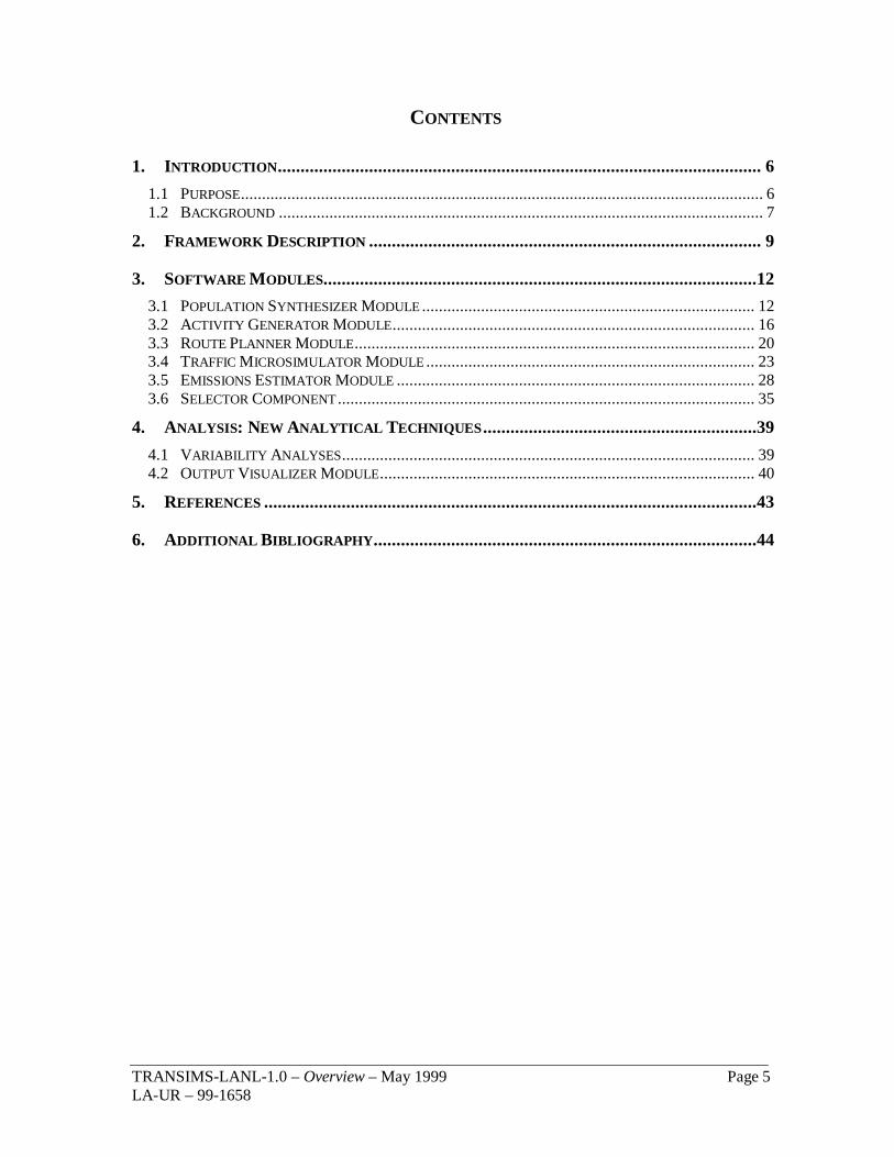
CONTENTS
1. INTRODUCTION.......................................................................................................... 6
1.1 PURPOSE............................................................................................................................ 61.2 BACKGROUND ................................................................................................................... 7
2. FRAMEWORK DESCRIPTION ...................................................................................... 9
3. SOFTWARE MODULES...............................................................................................12
3.1 POPULATION SYNTHESIZER MODULE ............................................................................... 123.2 ACTIVITY GENERATOR MODULE...................................................................................... 163.3 ROUTE PLANNER MODULE............................................................................................... 203.4 TRAFFIC MICROSIMULATOR MODULE .............................................................................. 233.5 EMISSIONS ESTIMATOR MODULE ..................................................................................... 283.6 SELECTOR COMPONENT ................................................................................................... 35
4. ANALYSIS: NEW ANALYTICAL TECHNIQUES............................................................39
4.1 VARIABILITY ANALYSES.................................................................................................. 394.2 OUTPUT VISUALIZER MODULE......................................................................................... 40
5. REFERENCES ............................................................................................................43
6. ADDITIONAL BIBLIOGRAPHY....................................................................................44

TRANSIMS-LANL-1.0 – Overview – May 1999 Page 6LA-UR – 99-1658
1. INTRODUCTION
1.1 Purpose
This document provides a high-level, conceptual overview of the TRANSIMS software package.It explains the end-to-end capability of TRANSIMS by describing the major data that must beprepared, the major software methods that use these data, and the major output data produced bythe software. The document is intended as a primer for potential end users and potential softwarevendors who might package the system for long-term use. This document does not provide adetailed description of individual data items or data structures, nor does it provide a detailedalgorithmic description of the software methods. These more-detailed descriptions are providedvia the Internet at http://transims.tsasa.lanl.gov.
TRANSIMS has flexible data requirements and modular software methods, along with multiplehardware and software operating environments. All of the modules in TRANSIMS are uniformlybased on the representation of individual synthetic travelers. Accordingly, TRANSIMS is moredata- and computation-intensive than existing methods. However, it is possible to begin the useof TRANSIMS by converting existing data to TRANSIMS formats and using minimallyconfigured hardware. Some existing issues can be adequately addressed in this manner. Mostissues, however, will demand more extensive data sets and more powerful computingenvironments to realize the full power of TRANSIMS. These needs are described in the nextsection. Over time, TRANSIMS modules and methods within those modules can be replaced bynew, more powerful methods developed by users and researchers. These new methods will workwell with other TRANSIMS modules provided that the framework data and communicationprotocols connecting modules and methods are followed.

TRANSIMS-LANL-1.0 – Overview – May 1999 Page 7LA-UR – 99-1658
1.2 Background
The goal of the TRANSIMS project has been to conduct major research and development offundamentally new approaches to travel forecasting. TRANSIMS emphasizes and quantifiesaspects of (1) activity-based travel demand, (2) intermodal trip planning, (3) trafficmicrosimulation, and (4) air quality and other macro analyses within the single, unifiedarchitecture shown in Figure 1.
Figure 1 The highest level view of TRANSIMS consists of four major modules: ActivityGenerator, Route Planner, Traffic Microsimulator, and Emissions Estimator. Feedbackbased on the modules is used to re-plan and modify activity demand and as a modeling tool.Multiple analyses, in addition to air quality analyses, can be performed usingmicrosimulation results.
TRANSIMS departs from traditional demand forecasting and impact analysis methods commonlyin use. New technical approaches in TRANSIMS respond to issues derived from legislation suchas the Intermodal Surface Transportation Efficiency Act and the Clean Air Act. Transportationplanning issues requiring new technical approaches include (1) congestion pricing, (2) alternativedevelopment patterns, (3) transportation control measures, and (4) motor vehicle emissions. Inaddition, major programs such as the Intelligent Transportation System require new TRANSIMSanalytical approaches for substantive evaluation of their effectiveness.
A major TRANSIMS technical feature is that the identity of individual synthetic travelers ismaintained throughout the entire simulation and analysis architecture. All synthetic travelers aregenerated as part of a synthetic population developed for a specific metropolitan region using avariety of data sources including census, surveys, etc. Activity times and locations are computedfor each individual. The plans generated by the Route Planner maintain individual identities, asdoes the Traffic Microsimulator. The resulting simulation output can provide a detailed, second-by-second history of every traveler in the system over a 24-hour day. A variety of impactanalyses can be conducted using these results. This approach relies on a simple, consistentarchitecture—one that provides planners with deeper insight into the underlying, second-by-second dynamics of the traffic system under different local (e.g., traffic signals) and global (e.g.,congestion) conditions.
Householdsand
Activities
Routesand
Plansµsimulation
EmissionsMODELS3

TRANSIMS-LANL-1.0 – Overview – May 1999 Page 8LA-UR – 99-1658
TRANSIMS consists of a series of building blocks or modules that produce populations,activities for populations, routes for travelers, and microsimulated traffic dynamics. TheTRANSIMS framework allows these modules to be executed in any desired order by a set ofselector scripts. As each module is executed using the framework with the selector scripts,chosen data is collected in an iteration database to be used by the other modules. This allows forinformation from, say, the microsimulated traffic dynamics to be fed back to the route generatorto produce a new set of more realistic routes for selected travelers.
Feedback and the control of feedback is an important function of the framework. One of thefunctions of feedback is to stabilize the results. As in assignment methodologies, the RoutePlanner may place more vehicles on links than the capacity of the link may allow. This maycause congestion to spill back onto other links. Results of the microsimulation in these cases canbe fed back to reroute selected travelers to stabilize this situation. The other function of feedbackis to model various aspects of transportation systems such as Intelligent Transportation Systems(ITS) implementations. Many ITS applications involve the movement of traffic information toselected travelers. Feedback accomplishes this.
The modules of TRANSIMS can be easily replaced or modified without redoing the entireTRANSIMS framework. Additionally, new modules may be added without much trouble. Forexample, a refined vehicle ownership module could be created to assign vehicles to an alreadycreated synthetic population without any change in the TRANSIMS framework.

TRANSIMS-LANL-1.0 – Overview – May 1999 Page 9LA-UR – 99-1658
2. FRAMEWORK DESCRIPTION
The TRANSIMS framework is shown in more detail in Figure 2 and Figure 3.In
put F
iles
Mod
ules
Inpu
t & O
utpu
t F
iles
PopulationSynthesizer
TravelerSurvey
SyntheticPopulation
Census
RoutePlanner
Activity
ActivityGenerator
OutputVisualizer
Traffic Micro-simulator
EmissionsEstimator
Network
TravelerPlans
Transit
VehicleSimulation
OutputEmissionsInventory
Arbitrary BoxData
MODELS3Database
Air QualitySurveys
Figure 2: The TRANSIMS architecture from the perspective of data flow. The majorTRANSIMS modules are represented in the middle row as boxes. Each of the TRANSIMSmodules depends on external data that are shown in the top row. Data produced by themodules, depicted along the bottom row, are used as input to other modules. The flow ofdata is controlled by the framework as shown in Figure 3.
ActivityGenerator
filter, sort,m
erge
,n
oise
reassigntravelers
SummaryOutput
TravelerEvents
Activity Set
RoutePlanner
Traffic Micro-simulator
update
Plan SetIteration
Database
new activities
replantravelers
merg
e/update
filter, sort,m
erge,noise
new plans update
filter, sort,m
erge,noise
new output
SyntheticPopulation
PopulationSynthesizer
selector
resimulatetravelers
roll back time, or pause
SelectorStatistics
update
update
EmissionsEstimator
EmissionsInventory
filter, sort,
merge,
noise
updatenew emissionsrecalculateemissions
arch
ive
Figure 3: TRANSIMS framework diagram with the Selector at the left.

TRANSIMS-LANL-1.0 – Overview – May 1999 Page 10LA-UR – 99-1658
This section provides an overview of the framework by emphasizing the flow of data andcomputation. From left to right, Figure 2 focuses on a single pass, feed forward data flow tosimplify the explanation of the process. This flow is controlled by the framework and a series ofselector scripts. Figure 3 describes the framework with the Selector component. The frameworkis the series of modules and their file interfaces. The Selector controls the flow of informationamong the modules. This flow may be as simple as the feed-forward depicted in Figure 2, or itcould be as complex as a series of feedback loops that takes data that have been produced by oneof the modules and stored in the iteration database and selectively feeds them back for iterativecomputation by the Activity Generator and Route Planner modules.
A single feed forward pass through the TRANSIMS framework, as shown in Figure 2, beginswith the preparation of a synthetic population data file for the metropolitan area. Although avariety of data sources can be used as input to the Population Synthesizer, to date we have usedthe following census data as sources:
1) U.S. Census Bureau Public Use Microdata Samples (PUMS)
2) U.S. Census Bureau STF-3A data
3) MABLE/GEOCORR data
The first two sources are available on CD-ROM from the Census Bureau; MABLE/GEOCORR isavailable over the Internet at the following web site location:http://plue.sedac.ciesin.org/plue/geocorr. The Population Synthesizer also uses land use data tolocate households relative to the transportation network.
The second data input required is the TRANSIMS networks. In contrast to most existing networkrepresentations, network data requirements for TRANSIMS are more detailed and contain moredata. TRANSIMS networks contain information similar to a TRANSYT-7F networkrequirements and include features such as the number of lanes, presence of turn pockets andmerge lanes, lane-use restrictions, high-occupancy-vehicle lanes, turn prohibitions, and speedlimits. Data on the location and type of signalized intersections are also required to producerealistic traffic flows.
The TRANSIMS networks may be viewed as “layered,” where each mode is represented by alayer of the network. TRANSIMS allows walking as a travel mode (the Route Plannerdetermines appropriate time delays for walking, but pedestrian movement is not microsimulated).Accordingly, a network especially for walking may be included in the TRANSIMS networks datafile. A useful, quick way to develop a walking network is to consider it as a subset of theroadway network. Transit data are incorporated when appropriate. The information contained inthis file provides the routes, operating schedules, and capacities for each transit asset (e.g., a busor light rail train). Each link on the vehicle network may be assigned zero to many parkinglocations. Finally, zero to multiple activity locations may be assigned to links of any type. Landuse data is associated with the activity locations. These data are used to determine the locationsof specific activities.
Not all traffic in a metropolitan area is caused by residents of that area. Non-Residential Traveldata include information on freight movements and itinerant travelers (i.e., those travelers passingthrough the metropolitan region whose trips originate outside the region). Currently, thisinformation is derived by using the same methods that generate trip tables for these types of tripsin the four-step process.

TRANSIMS-LANL-1.0 – Overview – May 1999 Page 11LA-UR – 99-1658
The Activity Generator module takes as major input the households in the synthetic population,local area surveys, Non-Residential travel data, TRANSIMS networks, and land use data. TheActivity Generator produces a list of activities for each traveler in the system and for each freight-hauling truck. For travelers contained in the synthetic population, activity patterns and modechoice preferences are derived from surveys. This derivation depends on demographicinformation contained in the synthetic households. Locations for the activities of each travelerare currently chosen by using methods derived from gravity models.
The Route Planner module attempts to produce plans for every individual and freight shipmentlisted in the activities list. The Route Planner computes a shortest or least-cost path for eachtraveler. If mode preferences are recorded for the traveler, the Route Planner ensures that theseare met and that the plan contains the required modal legs. The Route Planner estimates the timethat it takes to make a trip based on link traversal time estimates contained in the TRANSIMSnetworks or in simulation output. The Route Planner uses household vehicle information derivedfrom the synthetic population data file and transit service from the transit routes, stops, andschedules.
The Traffic Microsimulator module simulates the travel of individual vehicles and travelers inaccordance with the plans provided by the Route Planner. Each plan has a specified start time,which begins the execution of movement for that traveler. Plans that overlap in time are executedsimultaneously by the Traffic Microsimulator. The interactions of travelers and vehicles on thevarious networks over time create traffic flow dynamics. A one-second update interval ensuresthat dynamic vehicle behaviors (e.g., acceleration, deceleration, mode transfer, and signalintersection behavior) are captured with enough fidelity to generate realistic overall trafficbehavior.
The Emissions Estimator module uses results from the microsimulation to predict tailpipeemissions for light- and heavy-duty vehicles. Pollution from spilled fuel evaporation is alsoestimated. These emissions are aggregated to provide input to the MODELS-3 system to produceoverall Regional Air Quality estimates.
The Selector component, shown in Figure 3, is the primary mechanism used to achieve internalconsistency (i.e., to achieve a reasonable agreement among the travel demands expressed in theactivities list, the travel plans to meet these demands, and the execution of the plans in themicrosimulation) among the various computational modules. It selectively feeds backinformation from one module to another. For example, results from the Traffic Microsimulatormay be fed back to the Activity Generator or the Route Planner. In effect, this information isused to modify some designated subset of activities and/or plans to achieve realistic overall trafficresults.
Different versions of each module have been developed during the research process. Thedifferences range from minor changes in factors or values to completely different techniques.TRANSIMS is designed to accommodate and encourage the use of different modules both duringthe research process and in later commercial versions. This design, or Framework, will facilitatethe development and use of new modules and, ultimately, a stronger modeling package. Anexample of two completely different techniques for activity generation is discussed in Section3.2.2.

TRANSIMS-LANL-1.0 – Overview – May 1999 Page 12LA-UR – 99-1658
3. SOFTWARE MODULES
3.1 Population Synthesizer Module
The Population Synthesizer module builds virtual households for a given metropolitan area.These households are statistically derived from and consistent with available baseline informationsuch as standard census data and public use microdata samples.
3.1.1 Population Synthesizer Data Input/Output
PopulationSynthesizer
STF-3Aé summary tables of
demographicsé available at census tract and
block group levels of detail
PUMSé 5% sample of census recordsé PUMA consisting of census
tracts, etc.é approximately 5,000
individuals
TIGER/Lineé using MABLE/Geocorré geographic layout of census
tracts and block groups
Network Dataé activity locations
Synthetic Householdsé locationé block group
Synthetic Personsé genderé ageé schoolingé employment (type, location,
hours)é transportationé income
Vehiclesé vehicle idé householdé initial network locationé type of vehicle
Figure 4: The Population Synthesizer uses the following source data: (1) U.S. CensusBureau Public Use Microdata Samples (PUMS); (2) U.S. Census Bureau STF-3A data; (3)MABLE/GEOCORR; (4) land use data; and (5) TRANSIMS networks. The first twosources are available on CD-ROM from the Census Bureau; MABLE/GEOCORR isavailable over the Internet at the following Web site location:http://plue.sedac.ciesin.org/plue/geocorr. The major output of the modules is a syntheticpopulation of households containing a set of information associated with each householdand household locations within the TRANSIMS networks. Forecast populations used forplanning studies must contain information similar to Census STF-3A data.

TRANSIMS-LANL-1.0 – Overview – May 1999 Page 13LA-UR – 99-1658
3.1.2 Population Synthesizer Module Description
Any viable source of household and demographic data can be used to construct a syntheticpopulation, provided that the output of the computation is formatted in accordance withTRANSIMS data formats for synthetic populations (see TRANSIMS, Volume 3—Files athttp://transims.lanl.gov. A separately released software package called TRANSIMS: SyntheticPopulation is available. This package allows users to experiment with and build syntheticpopulations using census data.
Synthetic populations contain households comprised of one or more individuals. Each individualhas an associated set of demographic variables (e.g., age, sex, income, etc.) Households areusually generated for small areas such as census block groups or census tracts. Households areassigned to activity locations on a link of the TRANSIMS network according to land usecharacteristics associated with the activity locations on that link. If a walk network is used, it isuseful to assign households to activity locations on walk links only. It should be noted thatmultiple activity locations can be assigned to one link. In particular, an activity location on a linkcan represent one side of a street, while a second could represent the activities that take place onthe other side; activity locations might even represent individual buildings on a street. Syntheticpopulations provide input to the Activity Generator. Information contained in syntheticpopulations can also be used to categorize and filter subsets of the population used for varioustypes of equity analyses.
In the methodology presented here, each household in a synthetic population is classified as eitherfamily, non-family, or individuals living in group quarters such as dorms. Family householdscontain one or more adults and possibly children. Demographics associated with members ofhouseholds vary in accordance with source data and study needs. At a minimum, a TRANSIMShousehold must contain at least one person.
An example of how to generate a synthetic population is outlined in the paper by Beckman,Baggerly, and McKay, 1996 [1]. This technique uses the 1990 census data given in CensusStandard Tape File 3A (STF-3A) and PUMS. STF-3A gives demographic summary data on acensus tract or census block group level. The PUMS data is comprised of complete censusrecords, without any identification data such as name, address, census block, block group, ortract. PUMS covers 5% of the households surveyed over a large number of block groups. Thearea over which the PUMS ranges is called the Public Use Microdata Area (PUMA). The blockgroups that compose a PUMA are obtained from MABLE/GEOCORR, a geographiccorrespondence engine available at web site http://plue.sedac.ciesin.org/plue/geocorr.

TRANSIMS-LANL-1.0 – Overview – May 1999 Page 14LA-UR – 99-1658
Figure 5: The first step of constructing a synthetic population is to use PUMS data andstandard census data STF-3A. PUMS contains a 5% sample of real census records thathave been modified to maintain anonymity. These are used in conjunction with STF-3Asummary data, which contains demographic information.
The construction of a synthetic population is accomplished in several steps. First, an appropriatePUMA is identified, then MABLE/GEOCORR is used to obtain a listing of block groups withinthe PUMA (see Figure 5). Next, summary statistics from STF-3A for each of the block groupsidentified in the PUMA are obtained. As an example, summary data might include the age of thehouseholder, the family income, the number of workers in the family, the race of the householder,and the type of family. A multidimensional table is constructed from the PUMS data where thedimensions correspond to the summary statistics from STF-3A. In the example above, themultidimensional table would have five dimensions corresponding to five classifications: the ageof the householder, the family income, the number of workers in the family, the race of thehouseholder, and the type of family. The numbers of households in the PUMS for eachclassification compose the multidimensional table. The proportion of households for eachclassification for the block groups is unknown—they are determined by a two-stage iterativeproportional fitting procedure outlined in Beckman, Baggerly, and McKay, 1996. This proceduresatisfies the distributions of the STF-3A data for each block group while maintaining thecorrelation structure of the table constructed from the PUMS. A forecast population can begenerated using the same techniques, but replacing the STF-3A data with forecast STF-3A data.

TRANSIMS-LANL-1.0 – Overview – May 1999 Page 15LA-UR – 99-1658
Figure 6: Creating households and placing them on the network involves randomlyselecting actual PUMS households in accordance with the proportions derived from theIterated Proportional Fitting method.
The final two steps in population generation are (1) selection of households from the PUMS tomatch the constructed tables, and (2) placement of the households on links in the network. Anestimated proportion of households for each block group in each category of themultidimensional table is obtained from the iterative proportional fitting procedure. Thesynthetic population is formed for each block group by randomly selecting households from thePUMS according to these proportions.
Households are selected from the PUMS to match the number of households in the Census over agiven geographic area such as a block group or a census tract. Land use information is used toplace each household within a block group at an activity location on a walk link. Land use data isstored in the network activity location file. At a minimum, this file contains the identity of theactivity locations, their locations, the corresponding block group and census tract, and someindication of the activities that may be performed at that location. For the Portland Metro casestudy, this information is represented by the area (in square feet) of land use types surroundingthe link containing the activity location. Here, land use information includes the square footageof commercial, industrial, multi-family, and single-family residential property surrounding thelink. Additionally, the number of employers and the total number of employees around the linkare included in this file. The data in the file may be generated using aggregated data byconsidering the proportion of area around the link when compared to the total area represented bythe aggregated data.

TRANSIMS-LANL-1.0 – Overview – May 1999 Page 16LA-UR – 99-1658
To place households from the synthetic population at an activity location on a link, the linkswithin a block group are first identified. For Portland, weights for each activity location aredetermined by adding the residential square footage and a multiple of the multifamily squarefootage. Each individual weight for an activity location is divided by the total of the weights ofall of the activity locations in the block group. These ratios are used as the probability of ahousehold being located on a link. For each household, a random link (based on the probabilities)is selected, and the household is placed on that link. Note that households need not be placed atunique activity locations. Many households can share the same activity location. This householdlocation algorithm may remain the same no matter which area is being studied. However, theweights given to the activity locations in a block group will depend on the quality and availabilityof land use data.
Households may be located on a link by other techniques. For example, census block data couldbe used to determine the number of households in a block, and this number could then beassociated with an activity location on the link. Another possibility is to use electronic phonebooks or aerial photography to determine this number. Neither of these techniques has been usedto date in TRANSIMS case studies.
Each generated household is comprised of individuals. The household and individualdemographics are as rich as the data in the PUMS. Since the household is a replica of ahousehold in the PUMS, every variable in the PUMS is also associated with the household. Thisincludes, but is not limited to, the household structure, the individual and household incomes,individuals’ races and ages, those individuals who work, and those who attend school.
At this time, the vehicle ownership is given by the number generated from the syntheticpopulation procedure using the PUMS. A more refined vehicle ownership model based onpopulation demographics and network characteristics could be implemented and called in theframework after the synthetic population is generated. In both cases, each vehicle is an entry inthe vehicle file described in TRANSIMS Volume 3—Files. This file contains the TRANSIMSvehicle identification number, the household to which it is assigned, and the vehicle emissionstype. The emissions type is used in the Emissions Estimator module to determine emissions. Itreflects the operating condition of the vehicle, its type, and age. Presently, these vehicle types areassigned at random according to a national distribution of 23 vehicle emission types that aredescribed in the Emissions Estimator section of this document. In the future, the analyst maywish to utilize a vehicle type model based on Department of Motor Vehicle statistics, inspectionand maintenance records, and the synthetic population.
3.2 Activity Generator Module
The Activity Generator module computes a list of activities for each traveler and each freightmovement. Each activity in the list has an associated activity type, location, and time. Anymethodology may be used to generate the TRANSIMS activities as long as the activities areTRANSIMS compatible—that is, if each member of the synthetic population is assigned a set ofactivities and these activities are stored in an activity file in the format outlined in TRANSIMSVolume 3—Files. In this document, we describe two methods for generating TRANSIMSactivity files. One is being developed by the National Institute of Statistical Sciences (NISS) forthe Los Alamos National Laboratory, while the other is work performed for Portland Metro.

TRANSIMS-LANL-1.0 – Overview – May 1999 Page 17LA-UR – 99-1658
3.2.1 Activity Generator Major Input / Output
ActivityGenerator
Household ActivitySurvey
é representative sample ofpopulation
é including travel and activityparticipation of all householdmembers
é recorded continuously for 24+hours
Network Dataé nodesé linksé activity locations (includes
land use and employment)
Synthetic Population
Activitiesé participantsé activity typeé activity priorityé starting time, ending time,
duration (preferences andbounds)
é mode preferenceé vehicle preferenceé possible locations
Figure 7: The Activity Generator uses the synthetic population and non-residential traveldata to compute an activity list for every traveler and freight movement. This listconstitutes the travel demand for the region under study. Surveys are used to determineactivity patterns for households in the synthetic population.
Each TRANSIMS household member is assigned a set of activities for a 24-hour period. Theseactivities are based on models developed from activity surveys that are collected by metropolitanplanning organizations. The activity surveys generally ask respondents to list the householddemographics and to report the location, type, and duration of their activities over one or a multi-day period. The survey is used to develop activity patterns for households of various types.
The output of the Activity Generator is a data file containing the activities for each individualtraveler. This file identifies an individual and his/her corresponding household. Each individualis given a list of activities with the following attributes: type (e.g., home, work, shopping, school,or any other activity type collected in the survey), starting time range, ending time range, andactivity duration range.
3.2.2 Activity Generator Description
TRANSIMS assumes that any two activities, separated by time and location, require travelbetween them. The degree of detail in both the synthetic population and activities can varydepending on the availability of data and the study being performed. A more detailed study withmore realistic traffic can be accomplished with a more detailed and realistic representation of the

TRANSIMS-LANL-1.0 – Overview – May 1999 Page 18LA-UR – 99-1658
metropolitan population and the activities in which the population engages. The only requirementis that the file structure protocols are not violated. This section outlines the structure of theactivities, the methods for generating them, the minimum data required to execute TRANSIMS,and other sets of data that may be required by some TRANSIMS analyses.
Consider the following example: A person may need to arrive at work between 7:30 and 7:45a.m. and stay until 11:45 a.m. to noon. The starting time range in the activity list would be 7:30to 7:45; the ending time, 11:45 to 12:00 with a duration of 4 to 4.5 hours. The time information isa redundant set; consequently, not all of the fields (start time, end time, and duration) need to becompletely specified. Each activity has a location specified in the file, which must be part of theTRANSIMS network data file. The location is one of the activity locations listed in the activitylocation network file. In addition to the time and location, a travel mode to reach the activity isalso assigned. The mode may be very specific (such as requiring a car), or it may be general,allowing the Route Planner to search for the best mode(s) out of all possible modes. If two ormore individuals are making the same trip, in a particular driving trip, the individuals areidentified as part of the activity list.
One technique for activity generation, the NISS methodology, involves overlaying each synthetichousehold with a complete activity pattern. This is accomplished in the following way: Anactivity survey is processed to obtain the total time spent in activities by activity type for eachsurveyed household. These times are weighted and summed to form a measure of total time spentin activities for each household. Demographic variables of the household and the individuals inthe household are chosen based on which ones make the best predictors of the activity durationtime. The predictor takes the form of a decision tree where questions are asked at every level ofthe tree. (See Figure 8)
workers = 0all households
workers = 1
workers = 2
workers >= 3
persons = 1
persons = 2
persons >= 3
persons = 1
hhage < 38.5
hhage >= 38.5
hhage < 53
income > 5.5
income < 5.5
hhage >= 53
persons = 2 ages5to17 = 0
ages5to17 = 1
ages5to17 <= 1persons = 3 hhage < 29.5
hhage >= 29.5
ages5to17 >= 2
persons = 4 ages5to17 <= 1
ages5to17 >= 2
persons >= 5 ages5to17 <= 2
ages5to17 >= 3
persons = 2
persons = 3
persons >= 4 hdensity < 1.295
hdensity >= 1.295
persons = 3
persons >= 4
Figure 8: An example of a decision tree used to classify household activity patterns.

TRANSIMS-LANL-1.0 – Overview – May 1999 Page 19LA-UR – 99-1658
For example, the first question may be “is the household size equal to one?” The next level ofquestion for single person households may be “is the person a worker?” while the next level ofquestion for a multiple-person household might be “are there more than two people in thishousehold?” The tree ends at what are called terminal nodes, which specify the activity patternfor the household.
Once a decision tree is constructed, each household from the survey is classified as belonging toone of the terminal nodes of the tree. More than one household is usually assigned to each of theterminal nodes. Base activity patterns are allocated to individual households in the syntheticpopulation by classifying them according to the decision tree and giving them an activity patternof one of the survey households that were similarly classified as belonging to that node. Theactivity pattern is screened and corrected for obvious errors, such as a two-year-old personworking or having to drive. Given the base activity pattern, the locations of the activities aredetermined by a modified gravity model based on land use data in the activity location file. ForPortland, these are the square footage of commercial and industrial property around activitylocations on the link and the number of employees and employers assigned to the activitylocations on the link. Initial activity start and end times are determined from network skim timesfor travel from one area to another.
A second approach to TRANSIMS compatible activity generation is being developed by PortlandMetro. Using nested logit models with the parameters estimated from the Portland survey data,primary tours are assigned to individuals in the population. Some primary tours are home-to-work, work-to-home, and home-to-shop. After the primary tours are assigned to the individuals,secondary tours and intermediate stops on a primary tour are assigned to the individual bysampling the tours from the survey. Times, locations, and mode choices are obtained usinggravity models.
The TRANSIMS Framework allows the activity sequence, times, and locations to be easilychanged by feedback from the Route Planner and the Traffic Microsimulator. There is a tradeoffbetween spending resources to make the activity list as correct as possible and correcting the listby feedback. This is an active area of TRANSIMS research. Hopefully, only a rough cut isneeded for the base activity list, and a refined list will easily emerge through feedback.
The importance of feedback to refine the activity list should not be underestimated. If it can beshown that feedback can improve an activity list so that extremely detailed activity models arenot necessary, then national survey data and data from other sources could be used to constructthe base set of activities. In this case, an extensive local survey would not be needed. FutureTRANSIMS research in this area is important and may reduce the cost of surveys formetropolitan areas.
At this time, freight and itinerant travelers are handled in TRANSIMS through trip tables, whichare derived from a portion of the four-step process. The lack of data and models in these twoareas makes this simplifying approximation necessary. This can be changed easily as betterfreight models are developed. Trip tables are transformed into TRANSIMS activities in thefollowing way. Individuals (not created as part of synthetic populations) are created as vehicledrivers, and one vehicle is created for each trip in the trip tables. There may be multiple triptables representing various types of vehicles. For example, numerous trip tables could be used torepresent trucks with different numbers of axles. A trip table must be available to accommodatethe microsimulation of itinerant travelers. In this version of TRANSIMS, a single vehicle is usedfor only one trip. If a new model generates a sequence of trips for, say, a single delivery truck,this would be implemented easily by creating an activity list with an activity at every stop. Each
TRANSIMS-LANL-1.0 – Overview – May 1999 Page 20LA-UR – 99-1658
truck (and bus) simulated in TRANSIMS is listed in the vehicle file. As with automobiles, trucksand buses are assigned an emissions type.
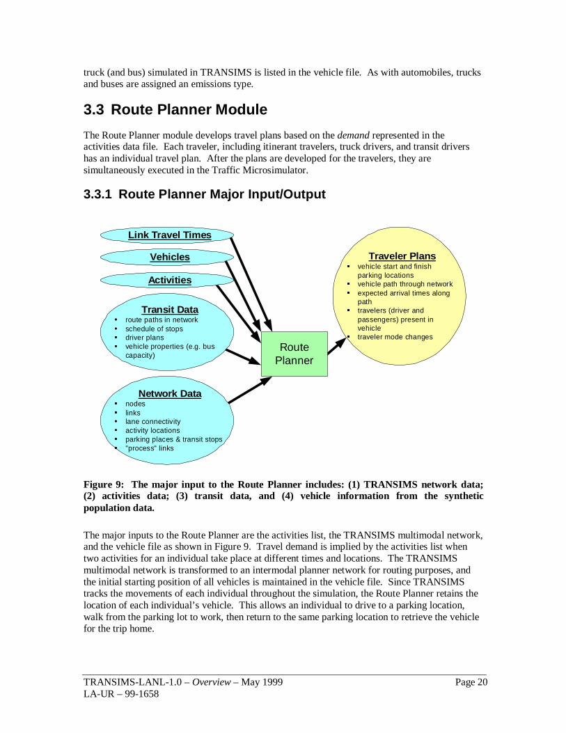
3.3 Route Planner Module
The Route Planner module develops travel plans based on the demand represented in theactivities data file. Each traveler, including itinerant travelers, truck drivers, and transit drivershas an individual travel plan. After the plans are developed for the travelers, they aresimultaneously executed in the Traffic Microsimulator.
3.3.1 Route Planner Major Input/Output
RoutePlanner
Transit Dataé route paths in networké schedule of stopsé driver plansé vehicle properties (e.g. bus
capacity)
Network Dataé nodesé linksé lane connectivityé activity locationsé parking places & transit stopsé "process" links
Vehicles Traveler Plansé vehicle start and finish
parking locationsé vehicle path through networké expected arrival times along
pathé travelers (driver and
passengers) present invehicle
é traveler mode changes
Activities
Link Travel Times
Figure 9: The major input to the Route Planner includes: (1) TRANSIMS network data;(2) activities data; (3) transit data, and (4) vehicle information from the syntheticpopulation data.
The major inputs to the Route Planner are the activities list, the TRANSIMS multimodal network,and the vehicle file as shown in Figure 9. Travel demand is implied by the activities list whentwo activities for an individual take place at different times and locations. The TRANSIMSmultimodal network is transformed to an intermodal planner network for routing purposes, andthe initial starting position of all vehicles is maintained in the vehicle file. Since TRANSIMStracks the movements of each individual throughout the simulation, the Route Planner retains thelocation of each individual’s vehicle. This allows an individual to drive to a parking location,walk from the parking lot to work, then return to the same parking location to retrieve the vehiclefor the trip home.

TRANSIMS-LANL-1.0 – Overview – May 1999 Page 21LA-UR – 99-1658
3.3.2 Route Planner Description
The Route Planner computes the shortest path for each traveler in the system, subject toconstraints. Each link within the network system has a cost associated with it. Costs for a linkcan be computed simply with input such as an estimated time delay. It can also be computed inmore sophisticated ways—for example, as a function of several variables including time delaysand actual monetary costs of the link, or including more abstract variables such as a penalty fortraveling through construction areas. Accordingly, shortest path can also be interpreted as leastcost. Constraints are provided by criteria such as mode preferences for different legs of the trip.
The Route Planner has several distinguishing features:
• First, plans are computed for each individual traveler in the population, based on thatindividual’s activity demands and preferences. This allows each traveler to have anindividualized view of the transportation system. Accordingly, costs associated with links inthe network are computed for each traveler.
• Second, link costs are computed in a time-dependent manner, which can account for timedelays resulting from actual travel conditions such as peak-hour congestion.
• Third, the Route Planner abides by any mode preferences contained in the activity files.Thus, if the activity files specify that a traveler will first walk, then take a car, and then walkagain between two desired activities, the Route Planner will produce a plan (if feasible) thatensures these modes are used in this sequence.
The Route Planner assumes the following definitions: A traveler plan is the set of trips thatcarries the traveler through his/her desired activities. Trips may be separated by activities thathave a given duration. A trip is a set of contiguous legs. A leg is a set of contiguous nodes andlinks that are traversed with a single travel mode. For example, a trip may consist of three legs,the first walking, the second transit, and the third walking; and a traveler plan could consist of atrip from home to work, work to shopping, then a trip from shopping to home.

TRANSIMS-LANL-1.0 – Overview – May 1999 Page 22LA-UR – 99-1658
walk
auto
bus
light railrail stop
bus stop
parking lot
activitylocation
pro
cess
lin
k
Figure 10: A high-level depiction of the various network levels used by the Route Planner.From individual traveler preferences and constraints contained in the synthetic populationand activities data blocks, the Route Planner must plan for trips comprised of multiplemodal legs (e.g., walk-car-walk). Constructing multiple network levels where each level canbe encoded as a different modal network allows for the efficient calculation of tripsconstrained by modal sequences. Also shown are the process links connecting the modalnetworks.
As shown in Figure 10, the Route Planner conceptually views the network as a set ofinterconnected, unimodal layers. That is, for each mode (e.g., walking, car, transit, etc.) aseparate network exists. At certain designated nodes in each of these networks, a special link,called a process link, exists to one or more of the other unimodal networks. These links allowintermodal transitions to occur. The process links are considered to be part of the walkingnetwork. The layered networks are constructed from the underlying network data representation.Traversal time for each link in each layered network is computed by a link traversal function,which is time-dependent.
The Activity Generator provides information on mode preferences for each trip. Conceptually,this information is captured in simple, alphabetical expressions. For example, a trip that containsa walking leg from a traveler’s house to his/her car, a car leg to parking at the place of work, anda walking leg from the parking lot to his/her actual work location would be represented as “w-c-w.” The Route Planner uses this information in the following way: For the first leg of the trip,the walking leg, the Route Planner searches for possible paths within the walking layer of thenetwork to obtain a walking route from the home to the parking location of the individual’svehicle. As soon as the walking path is found, a series of least-cost driving links is found toobtain a route to a parking location near the work location. A walk route is then developed tomove the traveler from the parking lot to the work activity location.
The last two legs of the above route highlight the capabilities of the Route Planner. Once thesearch algorithm is in the car network layer, it chooses additional links from the car network orparks the vehicle and chooses links from the walking network—whichever is lower in cost. TheRoute Planner ensures that the final link is a walking link in this example. Trips that cannot befeasibly planned are marked and provided as output from the Route Planner to be fed back to theactivity list to choose a new activity time or location or mode for travel to the activity.

TRANSIMS-LANL-1.0 – Overview – May 1999 Page 23LA-UR – 99-1658
3.4 Traffic Microsimulator Module
The Traffic Microsimulator module executes individuals’ travel plans link by link, as provided bythe Route Planner, at the start time specified by the plan. Plans that overlap in time are executedsimultaneously by the Traffic Microsimulator, resulting in overall transportation dynamics alongthe intermodal networks.
3.4.1 Traffic Microsimulator Major Input/Output
TrafficMicro-
Simulator
Transit Dataé route paths in networké schedule of stopsé driver plansé vehicle properties (e.g.
starting location)
Network Dataé nodesé linksé lane use and connectivityé intersections (signs and
signals)é activity locationsé parkingé transit stops
Traveler Plans
Traveler Eventsé traveler id, trip id, leg idé time, locationé inconvenience measuresé anomaliesé events
Summary Dataé link travel timesé link/lane densitiesé turn counts
VehiclesSnapshot Data
é vehicles on linksé vehicles in intersectionsé traffic controlsé vehicle sub-populations
Figure 11: The major inputs to the Traffic Microsimulator are the intermodal plans,transit data, TRANSIMS network data, and vehicle data.
The Traffic Microsimulator uses the TRANSIMS network and the intermodal plans asdiagrammed in Figure 11.
At a minimum, TRANSIMS network information must include the locations of streets andintersections, the number of lanes on the streets, the manner in which the lanes are connected, andsome parking locations on the streets at a collection of activity locations. Some studies mightbenefit from or require more detailed information about the network. Examples of more detailedstreet information that the Traffic Microsimulator is capable of using include the presence of turnpockets and merge lanes, lane use restrictions (such as high-occupancy vehicle lanes), turnprohibitions, and speed limits. Each intersection has a controller associated with it, which canvary from a stop or yield sign to a traffic signal, or to a set of coordinated traffic signals. Anotherkind of network information is the list of transit stops serviced by each route. The actual transitschedule is encoded in the travel plans of transit drivers. Transit drivers stop to pick up or dropoff passengers at transit stops.
For each traveler, the simulation must have a complete description of the traveler’s transportationplans. A plan is broken down into a sequential set of trips, which must begin and end at anactivity location, such as home, work, or shopping center. A trip is further decomposed into a setof unimodal legs. A traveler can use only a single mode of transportation on a leg. Accordingly,several legs are chained together to form a single trip.

TRANSIMS-LANL-1.0 – Overview – May 1999 Page 24LA-UR – 99-1658
3.4.2 Traffic Microsimulator Description
As a simulated day progresses, each person moves from one activity to the next according to thepredefined plan, using combinations of modes such as walking, driving a vehicle, and/or riding ina (private or public) vehicle. The Route Planner provides the link-by-link travel plan of thetraveler including the mode of travel. All TRANSIMS vehicles are simulated in detail to includedriving on roads, stopping for signals, accelerating, decelerating, changing lanes, stopping to pickup passengers, and so on. Mode changes—for example, from walking to car or to transit—areexplicitly simulated based on information contained in the traveler’s plan.
Vehicles follow a simple set of rules that guarantee that no collisions will occur. Phenomenasuch as reaction times and limited visibility are not simulated explicitly. However, the effects ofthese phenomena are simulated by the values of parameters used in the driving rules so that thefundamental flow-density diagram matches real, observed traffic.
The simulation can estimate the impact of hypothetical changes on quality of service. It providesanswers to such questions as the following:
• What would be the effect on traffic patterns of building a proposed highway?
• What is the impact of a change in transit schedules on riders?
• Can changing signalization alleviate congestion?
• Are there common demographic characteristics of the subpopulation most affected by aparticular infrastructure change?
The analytical power of the Traffic Microsimulator lies in aggregating the results of millions ofinteractions within the transportation system. These summaries focus on issues of interest such ascongestion and many other issues that can be addressed based on understanding very detailedtraffic flow information.
3.4.2.1 Single Trip Example
This example considers a work-to-home trip. It begins and ends at activity locations that arecoded in the TRANSIMS networks.
• Leg 1: walk from activity location W to bus stop X where W is the designation of the work activity location, and X is the designation of a bus stop in the network description
• Leg 2: take route Y to bus stop Z
• Leg 3: walk to parking lot P
• Leg 4: drive to day care at activity location D
• Leg 5: drive, with one passenger, to parking location P2
• Leg 6: walk to activity location H (home)
The first leg of this hypothetical trip is a walking leg. For walking legs, TRANSIMS does notexplicitly microsimulate the second-to-second locations of pedestrians. Based on information
TRANSIMS-LANL-1.0 – Overview – May 1999 Page 25LA-UR – 99-1658
contained in a given traveler’s plan, legs of a trip that involve walking will begin at the timespecified by the Route Planner at the point of origin for the leg and end at the destination of theleg. The traveler arrives at the destination at a simulation time computed by adding the delaytime (contained in the plan) to the start time for the walk mode leg. No additional information isrequired or generated for walk mode legs.
The second leg of the trip is a bus leg. A bus leg plan requires only one additional piece ofinformation: the acceptable route(s). The precise itinerary of the bus the traveler gets on isdetermined by the driver’s plan. The traveler simply waits until his desired stop is reached andexits the bus. Bus loading and unloading is represented explicitly by the microsimulation.Resource constraints such as vehicle capacity and parking lot capacity are observed. If a bus isfull when it reaches the bus stop, the traveler is not permitted to board and will wait for the nextbus on the same route. With this level of detail, it is easy to determine how many passengerscannot find space on the bus, or how many minutes a traveler must wait for a bus.
The next leg calls for the traveler to walk to the parking lot after getting off the bus. In thisinstance, the parking lot is where the traveler left his/her private vehicle. This walking leg ishandled as previously described.
Upon arriving at the parking lot, the traveler is associated with a specific vehicle, which musteither have been left in the parking lot earlier in the simulation or placed there duringinitialization. The traveler and car exit the parking lot into the traffic network. The traveler’splan specifies exactly which turns he/she will take until he/she arrives at the daycare center.Here, the traveler waits until his/her passenger enters the car. The passenger’s plan will specifywhat vehicle to ride in, and the passenger will be waiting for this vehicle to arrive. Then, asbefore, the driver re-enters the transportation network, following his/her plan, parks, and walkshome.
As described above, a transit schedule is implemented by providing plans for each transit driver.Like other travelers, a driver can switch vehicles, switch routes (with or without switchingvehicles), and take layovers of prescribed duration or ending time at specific control points.
The Traffic Microsimulator enforces physical constraints—travelers cannot be in two places atonce, and they cannot create vehicles. Thus, travelers and vehicles will be initialized and placedin their initial start locations based on information in the plan file.
3.4.2.2 Cellular Automata
Vehicle movement is accomplished using a cellular automata simulation. Each section ofroadway (see Figure 12) is divided into cells of a grid 1-lane wide by 7.5-meters long. Each celleither contains a vehicle (or a part of one) or is empty. The simulation is carried out in discretetimesteps, each simulating one second of real time. On each timestep, a vehicle on the networkdecides whether to accelerate, brake, or change lanes in response to the occupancy of nearby gridcells. After every vehicle is allowed to make these decisions, they are all moved to new grid cellsin accordance with their current velocity.

TRANSIMS-LANL-1.0 – Overview – May 1999 Page 26LA-UR – 99-1658
Figure 12: The roadway is divided into lanes, and the lanes are divided into cells. Eachlane’s possible turning movements at intersections are defined. Controls at intersectionsmanage traffic and maintain information about oncoming vehicles. Shown from theperspective of the middle peach-colored car, the gap (labeled 1 in the figure) betweenvehicles determines accelerations and influences lane changes. The gaps (2, 4 for left-lanechange, 6 for right-lane change) to vehicles in other lanes also influence lane changing. Thedistance at the intersection (3) determines the relative importance of changing lanes. Thegaps (4, 5, 6) to upstream vehicles from a parking facility determine whether vehicles canexit the parking facility.
As part of the lane-changing procedure, transit vehicles scan the nearby cells for transit stops,which they must service. The transit vehicles can examine the queue at the stop to see if anyoneis waiting for the vehicle and can also query their passengers to see if anyone wants to get out atthe stop. If so, they either stop in the cell next to the transit stop or pull off the grid, depending onthe type of transit stop. Passengers take a fixed time to enter or leave the vehicle.
Each intersection has traffic control logic, which controls entry of vehicles into the intersection.Traffic controllers examine the traffic in each lane at the intersection. If the intersection is clear,vehicles pass through it in a fixed amount of time and are placed on the next roadway’s grid.
Vehicles entering the roadway from parking locations or off-street transit stops can enter any lanewith a large enough gap between it and the oncoming traffic. The gap must be large enough toensure that on the next timestep, no vehicles will collide with vehicles entering the roadway.
The simulation guarantees that each vehicle makes decisions based on the state of every othervehicle in its local vicinity (i.e., 5 cells) at the same time. That is, every vehicle in the networkmakes its acceleration decision based only on information available at time t, which does notinclude the time t+1 positions of vehicles that have already made their acceleration decision.This parallel update scheme ensures that the simulation results do not depend on the order inwhich streets in the network are updated.

TRANSIMS-LANL-1.0 – Overview – May 1999 Page 27LA-UR – 99-1658
To accomplish the simulation update, a single timestep must be broken down into several parts.First, the vehicles at the head of a queue waiting to leave a parking location are allowed to enterthe road. Then, all vehicles are allowed to change lanes (in this step, transit vehicles are allowedto enter transit stops also). In order to avoid possible collisions when vehicles in two lanes attime t both try to change into the same lane, we alternate the direction of lane changing everytimestep. Next, those vehicles that will enter intersections are marked and given instructionsfrom the intersection controller about the availability of their destination link. Every vehiclemakes its acceleration decision, and all of the vehicles are moved. Finally, vehicles are allowedto exit into parking locations.
3.4.2.3 Traffic Microsimulator Output
There are four major kinds of output from the Traffic Microsimulator. Figure 13 shows summarydata (both spatial and temporal), traveler events, and snapshot data. Spatial summaries includedata aggregated over user-defined sections of roadway defined along the street networks—forexample, densities and total flow in a 150-meter section. Temporal summaries include data abouttravel times along streets at various times of day. Almost anything that happens to a traveler canbe reported as a time-stamped event in the event output. Commonly used events includebegin/end waiting at a given location, such as a bus stop, begin/end a leg, pass through anintersection, and enter a vehicle. If desired, traffic animation can be produced from the snapshotfiles, which contain time, position, and velocity information for each vehicle in the simulation.These files can also be used to recover data that has not already been provided in the summarydata files. For instance, if some new study requires the average gap between vehicles, it can becomputed from snapshot data.
Dumping out the snapshot data for a 24-hour simulation of a major metropolitan area createsextremely large files. Users are allowed to restrict output to smaller portions of the network andspecific times during the simulation, as well as to select only a few desired fields or only thoserecords that meet certain criteria. For example, a user may choose only specific events likebeginning a leg, only particular travelers, or only vehicles traveling above a given speed. Thesampling rate and reporting frequency for each of these data types is controlled by parametersselected by the user.

TRANSIMS-LANL-1.0 – Overview – May 1999 Page 28LA-UR – 99-1658
The state of eachvehicle on thelink is reported.
Snap-shotData
vehicle id, time, link id, position, velocitiy, lane, status
The stateof thetrafficcontrol isreported.
node id, time, phase, allowed movements
The state ofeach vehicle inthe intersectionis reported.
vehicle id, time, node id, position
Thetraversaltimes forvehiclesthat havetraveledthe lengthof the linkare summ-arized.
Summ-ary
Data
link id, vehicle count, sum of travel times
{
The vehicle counts and velocities in"boxes" along the link are summarized.
link id, box position, vehicle count, sum of velocities
The traveler hasjust become lostbecause he/shecannot make theleft turn he/sheplanned onmaking at thisintersection.This event isreported.
TravelerEvents
traveler id, vehicle id, time, location, event
Figure 13: The various types of Traffic Microsimulator output—traveler events, snapshotdata, and summary data—are depicted.
3.5 Emissions Estimator Module
The Emissions Estimator module translates traveler (vehicle) behavior into estimates of airquality, energy consumption, and carbon dioxide emissions. Four major computationalsubmodules compose the Emissions Estimator module: (1) emissions, (2) atmospheric conditions,(3) local transport and dispersion, and (4) chemical reactions. The MODELS-3 system,developed by the EPA, contains the last three of these and is not part of the TRANSIMSframework.

TRANSIMS-LANL-1.0 – Overview – May 1999 Page 29LA-UR – 99-1658
3.5.1 Emissions Estimator Major Input/Output
F l e e t S t a t u s
E m i s s i o n I n v e n t o r y
· N O X · C O · H C · P a r t . 3 0 m b y 1 5 m i n .
· C h e m i s t r y · T r a n s p o r t · D i s p e r s i o n
· O z o n e · P a r t . · N O 2 · C O · H C 3 - D c o n c e n t r a t i o n s h o u r l y h o r i z o n t a l r e s . 1 ” 5 k m v e r t i c a l r e s . 2 0 ” 5 0 0 m .
D e c e l s I n s i g
P l a n n e r T r u c k L o a d s
M i c r o - s i m u l a t i o n
R e s u l t s
V e h i c l e S y n t h e t i c
P o p u l a t i o n
1 1 , 2 , . . . , 1 2 1 3 1 4 , . . . , 2 5
2
4 0
D e c e l s A c c e l s
A c c e l s
1 1 2 3
2
4 0
R e g i o n a l A i r Q u a l i t y
L D V A g g r e g a t e D y n a m i c s
H D V A g g r e g a t e D y n a m i c s
E V A P
L D V T A I L P I P E
H D V T A I L P I P E
P o w e r D i s t . b y T i m e a n d
S e g .
F l e e t D y n a m i c s
P o w e r ( v / A D i s t . )
M O D E L S 3
Figure 14: Emissions Estimator data flow.
The data flow of the Emissions Estimator is summarized in Figure 14. The Emissions Estimatorrequires information on the fleet composition developed from the Population Synthesizer, vehicleloads, and traffic patterns. The Population Synthesizer provides vehicle fleet characteristicsincluding the fraction of the fleet that is malfunctioning. The traffic patterns are produced by theTraffic Microsimulator.
The bulk of the information required by the Emissions Estimator is produced by the TrafficMicrosimulator. The following items are included in this category:
1) spatial summaries of vehicle velocities over 30-meter sections of roadway
2) summaries of the gaps between vehicles as a function of vehicle speeds
3) histograms of the number of vehicles entering a link grouped by velocity-acceleration productsummed over time since the vehicles were parked
4) bus loads
Emissions Estimator output data is aggregated on 30-meter segments for each simulated 15-minute period. Fuel economy and CO2 emissions are also estimated. The emission inventory isdesigned to be used with the MODELS-3 code, developed by the Environmental ProtectionAgency (EPA) to produce three-dimensional, hourly, gridded emissions values over themetropolitan area.

TRANSIMS-LANL-1.0 – Overview – May 1999 Page 30LA-UR – 99-1658
3.5.2 Emissions Estimator Description
There are three major submodules in the Emissions Estimator:
1) Fuel Evaporation submodule
2) Light-Duty Vehicle (LDV) Tailpipe submodule
3) Heavy-Duty Vehicle (HDV) Tailpipe submodule
The Fuel Evaporation submodule treats emissions associated with resting losses, running losses,hot soaks, and diurnal pressure changes. It deals with both normally operating vehicles and withvehicles with significant leaks in the fuel system.
The LDV Tailpipe submodule treats tailpipe emissions from cars, small trucks, and sport utilityvehicles. Important aspects include:
1) malfunctioning vehicles
2) emissions from cold starts
3) emissions from warm starts in which the engine is still warm but the catalyst is cold
4) emissions from off-cycle conditions, conditions that occur outside those in the federal testprocedure, or that render the pollution controls inefficient
5) normal driving
The HDV Tailpipe submodule treats tailpipe emissions from trucks and buses. While truckemissions are not sensitive to power levels as are LDVs, their emissions are sensitive to the loadcarried by the vehicle.
3.5.2.1 Fuel Evaporation Submodule
The Fuel Evaporation submodule uses vehicle activity information generated by TRANSIMS andactivity-specific emissions models from the EPA to generate the evaporative emissions values. Ituses an age distribution of the vehicles in the simulation and includes the ratio of light-duty trucksto automobiles. The evaporative model provides values for outputs of hydrocarbons over 15-minute periods (interpolated from hourly values) on 30-meter segments along links, or at parkinglocations.
The Fuel Evaporation submodule uses information from the Traffic Microsimulator to determinethe location of a vehicle and whether it is presently operating or has operated in the previoushour. If the vehicle is not operating or has not operated in the last hour, resting losses and diurnalevaporative emissions are calculated for the vehicle using the vehicle categories and the equationsdeveloped for the Mobile 6 model of the EPA. These emissions are then assigned to the spatialgrid where the vehicle is located. If the vehicle is operating, running losses are calculated usingthe Mobile 5 formulation. If a vehicle has operated within the past hour, hot soak emissions arecalculated using the hot soak model developed by the EPA for Mobile 6.
For vehicles in the simulation area but not operating during the simulation period, diurnal andresting losses are calculated and assigned to the appropriate spatial location.

TRANSIMS-LANL-1.0 – Overview – May 1999 Page 31LA-UR – 99-1658
3.5.2.2 Light-Duty Vehicle Tailpipe Submodule
The Light-Duty Vehicle Tailpipe submodule treats emissions from off-cycle driving,malfunctioning vehicles, normal driving, idling, and vehicles with cold engines and/or catalysts.The LDV data flow is illustrated in Figure 15. Three major sets of information—fleetcomposition, fleet status, and fleet dynamics—are inputs to this submodule.
Figure 15: LDV Tailpipe submodule data flow.
3.5.2.2.1 LDV Tailpipe Fleet Composition
Fleet composition is given in the vehicle file from the Population Synthesizer. The 23 categoriesof vehicles in this file reflect such characteristics as engine-to-weight ratio and the catalyst type.
3.5.2.2.2 LDV Tailpipe Fleet Status
Fleet status is developed from the pattern of usage of the vehicles traversing a given link. Fuelconsumption is a function of the temperature of the engine and the catalyst. The TrafficMicrosimulator records when and where the vehicles have been operating on an individual-vehicle basis. Consequently, the fraction of the fleet in various phases of cold engine/coldcatalyst operation can be estimated from the vehicle origins and links traveled.
3.5.2.2.3 LDV Tailpipe Fleet Dynamics
Given good estimates of a vehicle’s continuous power output, its velocity, and the type of vehicle(provided in the synthetic population data file), predictive models of tailpipe emissions can bedeveloped. The principal component in estimating a vehicle’s continuous power is directlyproportional to the product of its velocity and acceleration. Thus, good estimates of thesevariables for the vehicles in a TRANSIMS microsimulation are extremely important to predictemissions.
The velocity of TRANSIMS LDVs is estimated in the following way: Since the microsimulationis a cellular automata, only a discrete number of vehicle velocities are possible. The

TRANSIMS-LANL-1.0 – Overview – May 1999 Page 32LA-UR – 99-1658
microsimulation vehicles can be moving an integer number, 0 to 5, cells per second. Theserepresent speeds of 0 to 7.5∗5=37.5 meters per second (or 0 to 84 miles per hour). For theEmissions Estimator, we summarize TRANSIMS velocity output over 15-minute intervals and30-meter segments (boxes) by counting the number of vehicles in each of the six speed bins, 0 to5 cells per second.
Because of the significant nonlinear character of the relationship between power and emissions, amore finely grained estimate of velocity is needed. This is accomplished by fitting a continuousmodel to the discrete data in the six speed cells that range from 0 to 37.5 meters per second.From this fit, the number of vehicles traveling at speeds in 2-mph increments is determined.
Next, vehicle accelerations are estimated. Data collected in the EPA’s three-city study, wheremany vehicles were fitted with a data logger that recorded times and speeds throughout thevehicles’ travels, are used. Frequency distributions of accelerations for given velocities weredetermined from these data. From these data, it was evident that the fraction of vehicles having avelocity-acceleration product greater than a specified level falls off exponentially with the level.
In the case of decelerations, the frequency also falls off exponentially with the velocity-deceleration product. These relationships form one of the principal empirical underpinnings inthe approach used here. All accelerations are placed in one of three groups: (1) hardaccelerations, (2) insignificant accelerations, and (3) hard decelerations. From empirical data andanalysis, hard accelerations are defined as those accelerations greater than the accelerationsassociated with the 10% of vehicles that have the largest velocity-acceleration product. Thenumber of vehicles undergoing a hard acceleration is estimated, and 12 different power levelsabove the hard acceleration cutoff are chosen to represent different levels of aggressiveness. Thetotal population of vehicles undergoing hard acceleration from a given speed is then distributedover the 12 power (or equivalently acceleration) levels. This data is used to estimate the relativeproportions of vehicles having different levels of acceleration within the group of vehicles thatundergo hard accelerations.
A second methodology to estimate the number of vehicles undergoing hard-acceleration,insignificant acceleration, and hard deceleration is being investigated. It is hypothesized that thefraction of vehicles undergoing hard acceleration would be related to average speed changesbetween segments or to the standard deviation of speeds within a segment. If most vehicles areaccelerating so that the average speed is increasing along the link, a higher proportion of hardaccelerations would be expected. On the other hand, if the average speeds are not changing butthere is a large standard deviation of speeds within the segment, slower vehicles would beaccelerating to regain their desired speed after encountering a temporary traffic jam. Thishypothesis was tested by examining data collected by the California Air Resources Board. Here,driving on freeways with seven different levels of congestion and driving on arterials with threedifferent levels of congestion were described. A simple two-parameter curve-fit was used torelate the probability of a hard acceleration to gradients in speed to the standard deviation ofspeeds within a link segment. In the calibration, only the fastest freeway, a mid-speed freewaythat had the highest standard deviation of speeds, and the fastest arterial that had a large gradientin speeds for vehicles leaving a signalized intersection were used. The relationships on theremainder of the arterials and freeways were tested, and good results were obtained. Therelationships are used to estimate the fraction of the vehicles undergoing hard acceleration,insignificant acceleration, and hard deceleration. The fraction of vehicles in the hard-accelerationgroup is distributed with the exponential distribution into 12 groups of velocity-accelerationproduct. Emissions are estimated for each velocity grouping (2-mph bins) and each accelerationgrouping (25 levels of 1.5 feet per second).

TRANSIMS-LANL-1.0 – Overview – May 1999 Page 33LA-UR – 99-1658
3.5.2.2.4 LDV Emissions Model
Barth et. al. [4] developed an improved modal emission model for LDVs. They carried outextensive tests on over 300 vehicles chosen to represent the major types of emitters in the existingLDV fleet. They also worked with other data to help draw associations between the testedvehicles and the fleet at large.
Using speeds and accelerations, the model computes the tractive power by taking into accountengine friction losses, rolling resistance, wind resistance, changes in kinetic energy, and changesin potential energy. It also considers the power to drive accessories such as air conditioning, andit estimates drive-train efficiency. With the engine power known, it calculates the rate of fuelconsumption and engine emissions. It treats enrichment, enleanment, and stoichiometricoperations, as well as cold-start operation.
Once the engine emissions are calculated, catalyst pass fractions are used to calculate the tailpipeemissions. The approach uses a composite vehicle to represent vehicles in the same class. Aregression approach was used to define the parameters required by the model. The vehicles wereall tested over cycles involving very high power demands and a variety of driving patterns.
There are composite vehicles representing normal-emitting cars categorized by technology, lowand high power-to-weight ratios, and mileages above or below 50,000. The technologycategories are (1) no catalyst, (2) two-way catalyst, (3) three-way catalyst with carburetion, (4)three-way catalyst with fuel injection, and (5) Tier 1. Only the last two categories are broken intomileage or power-to-weight ratio groupings. There are high-emitting composite vehicles fortechnologies (3) through (5), but they are not further subdivided into power-to-weight ratios ormileage groupings.
There are composite vehicles representing normal-emitting trucks with model year categories: (1)pre-1979, (2) 1979 to 1983, (3) 1984 to 1987, (4) 1988 to 1993, and (5) 1994 and newer. In agecategories (1) through (3), there is only a single composite vehicle. For age category (4), thereare categories for trucks above and below 3750 pounds loaded-vehicle weight, while for category(5) there is a category for trucks with loaded-vehicle weights between 3751 and 5750 pounds, anda category for gross vehicle weights between 6001 and 8500 pounds. There are compositevehicles representing high-emitting trucks for model years 1984 to 1987, 1988 to 1993, and 1994and newer. In the high-emitting category, there are no breakdowns by vehicle weight.
3.5.2.3 Heavy-Duty Vehicle Tailpipe Submodule
The Heavy-Duty Vehicle (HDV) Tailpipe submodule treats emissions from trucks and buses asthey idle or deliver loads about the city. Truck emissions are sensitive to power demandsassociated with accelerations, climbing grades, and hauling heavy loads. Bus emissions aresensitive to power demands, but loads play a relatively smaller role. Figure 16 describes the dataflow for the HDV Tailpipe submodule. There are three major sets of information that must bedeveloped: (1) fleet composition, (2) fleet status, and (3) fleet dynamics.
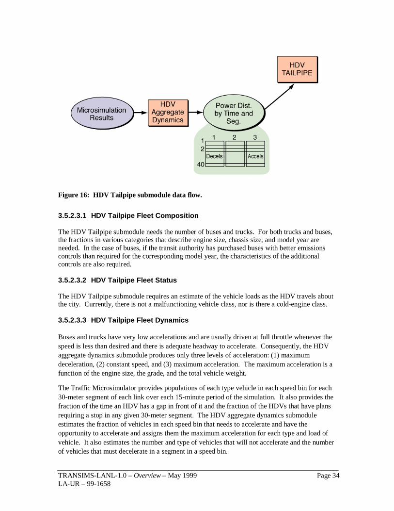
TRANSIMS-LANL-1.0 – Overview – May 1999 Page 34LA-UR – 99-1658
Figure 16: HDV Tailpipe submodule data flow.
3.5.2.3.1 HDV Tailpipe Fleet Composition
The HDV Tailpipe submodule needs the number of buses and trucks. For both trucks and buses,the fractions in various categories that describe engine size, chassis size, and model year areneeded. In the case of buses, if the transit authority has purchased buses with better emissionscontrols than required for the corresponding model year, the characteristics of the additionalcontrols are also required.
3.5.2.3.2 HDV Tailpipe Fleet Status
The HDV Tailpipe submodule requires an estimate of the vehicle loads as the HDV travels aboutthe city. Currently, there is not a malfunctioning vehicle class, nor is there a cold-engine class.
3.5.2.3.3 HDV Tailpipe Fleet Dynamics
Buses and trucks have very low accelerations and are usually driven at full throttle whenever thespeed is less than desired and there is adequate headway to accelerate. Consequently, the HDVaggregate dynamics submodule produces only three levels of acceleration: (1) maximumdeceleration, (2) constant speed, and (3) maximum acceleration. The maximum acceleration is afunction of the engine size, the grade, and the total vehicle weight.
The Traffic Microsimulator provides populations of each type vehicle in each speed bin for each30-meter segment of each link over each 15-minute period of the simulation. It also provides thefraction of the time an HDV has a gap in front of it and the fraction of the HDVs that have plansrequiring a stop in any given 30-meter segment. The HDV aggregate dynamics submoduleestimates the fraction of vehicles in each speed bin that needs to accelerate and have theopportunity to accelerate and assigns them the maximum acceleration for each type and load ofvehicle. It also estimates the number and type of vehicles that will not accelerate and the numberof vehicles that must decelerate in a segment in a speed bin.

TRANSIMS-LANL-1.0 – Overview – May 1999 Page 35LA-UR – 99-1658
3.5.2.3.4 HDV Emissions Model
West Virginia University investigators have carried out detailed studies using a chassisdynamometer on a variety of HDVs. For the TRANSIMS work, they have developed emissionsvalues for two different classes of buses under full throttle, constant speed, and deceleration in 2-mph increments from idle to 78 mph. They have also developed full-throttle trajectories for thebuses and have provided relationships to correct the trajectories for vehicle weight and grade.
The HDV model estimates emissions for the HDVs with specified loads, speeds, grades, andacceleration categories. The principal emissions of interest are NOx and fine particles, and theseare provided as 15-minute averages for each 30-meter segment of each link.
3.6 Selector Component
The process of iterative feedback is an important feature of TRANSIMS. It is the primarymechanism used to achieve internal consistency (i.e., to achieve a reasonable agreement amongthe travel demands expressed in the activities list, the travel plans to meet these demands, and theexecution of the plans in the Traffic Microsimulator) among the various computational modules.It selectively feeds back information from the Traffic Microsimulator into the Activity Generatorand Route Planner or from the Route Planner to the Activity Generator. In effect, thisinformation is used to modify a designated subset of activities and/or plans of the syntheticpopulation to achieve realistic overall traffic results. In addition, it allows the overallcomputational system to abstractly reflect learned behavior within the simulated populationrepresented. TRANSIMS synthetic travelers do not learn in the way humans do, but thistechnique emulates the ability of humans to learn from day-to-day experiences in order to avoidcongestion, etc. It also provides a way to model intelligent responses to information that may beprovided ultimately by Intelligent Transportation Systems (ITS) technologies.
The Selector controls the iterative process. A typical TRANSIMS study involves repeatediteration between components such as the Activity Generator, Route Planner, and TrafficMicrosimulator. There is no single, standard selector component, however, because differentstudy designs involve different iteration schemes. A variety of selectors have uses in differentstudies or other contexts.

TRANSIMS-LANL-1.0 – Overview – May 1999 Page 36LA-UR – 99-1658
Link SummaryOutput
Traveler EventOutput
Activity Set
update
Plan Set
IterationDatabase
merge/update
SyntheticPopulation
selector
SelectorStatistics
Network
arch
ive
ActivityGenerator
filter, sort,m
erge,noise
reassigntravelers
Route Planner
Traffic Micro-simulator
new activities
replantravelers
filter, sort,m
erge,noise
new plans update
filter, sort,m
erge,noise
new output
PopulationSynthesizer
resimulatetravelers
roll back time, or pause
update
update
ITS
filter, sort,m
erge,noise
updatenew networkadapt network
Figure 17: TRANSIMS framework diagram with the Selector at left.
The user can prepare a script to control the whole process of iteration. The script uses a specialcontrol language specifically developed for this component. It allows the user to filter results, runrepeated iterations, establish stopping criteria, and perform a variety of other operations that makethe analyst’s job less manpower-intensive.
At the beginning of each iteration, the iteration script controlling the current study typicallyinvokes the Selector. (The script might even use a different selector for each iteration in a study.)When the Selector runs, it usually will do the following:
• Read information about the travelers from the iteration database.
• Examine each traveler and decide whether to
� regenerate his/her activities using the Activity Generator,
� choose a new route between his/her existing activities using the Route Planner, or
� retain his/her existing activities and the planned route between them.
• Write the selections made for each traveler into data files that can be read by the ActivityGenerator and/or Route Planner when they are executed.
• Summarize the selections made and the current state of the system into the Selector statisticsdata file.
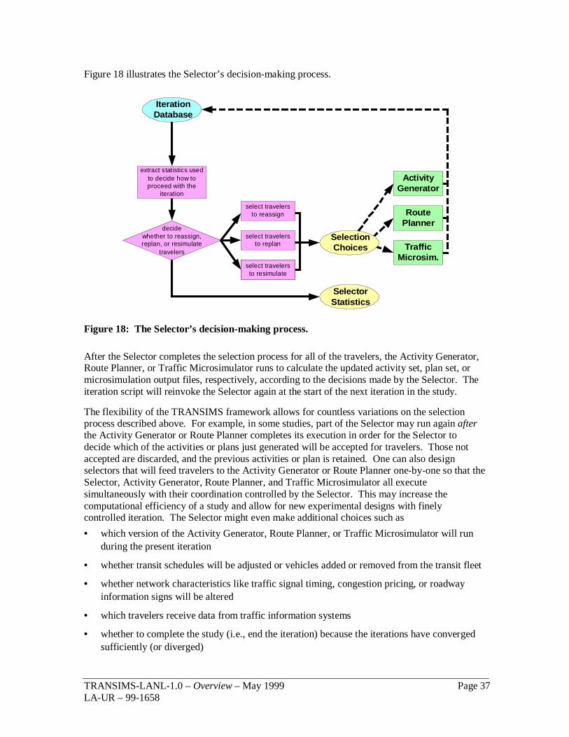
TRANSIMS-LANL-1.0 – Overview – May 1999 Page 37LA-UR – 99-1658
Figure 18 illustrates the Selector’s decision-making process.
select travelersto resimulate
IterationDatabase
SelectorStatistics
SelectionChoices
extract statistics usedto decide how toproceed with the
iteration
select travelersto reassign
decidewhether to reassign,replan, or resimulate
travelers
select travelersto replan
ActivityGenerator
RoutePlanner
TrafficMicrosim.
select travelersto resimulate
Figure 18: The Selector’s decision-making process.
After the Selector completes the selection process for all of the travelers, the Activity Generator,Route Planner, or Traffic Microsimulator runs to calculate the updated activity set, plan set, ormicrosimulation output files, respectively, according to the decisions made by the Selector. Theiteration script will reinvoke the Selector again at the start of the next iteration in the study.
The flexibility of the TRANSIMS framework allows for countless variations on the selectionprocess described above. For example, in some studies, part of the Selector may run again afterthe Activity Generator or Route Planner completes its execution in order for the Selector todecide which of the activities or plans just generated will be accepted for travelers. Those notaccepted are discarded, and the previous activities or plan is retained. One can also designselectors that will feed travelers to the Activity Generator or Route Planner one-by-one so that theSelector, Activity Generator, Route Planner, and Traffic Microsimulator all executesimultaneously with their coordination controlled by the Selector. This may increase thecomputational efficiency of a study and allow for new experimental designs with finelycontrolled iteration. The Selector might even make additional choices such as
• which version of the Activity Generator, Route Planner, or Traffic Microsimulator will runduring the present iteration
• whether transit schedules will be adjusted or vehicles added or removed from the transit fleet
• whether network characteristics like traffic signal timing, congestion pricing, or roadwayinformation signs will be altered
• which travelers receive data from traffic information systems
• whether to complete the study (i.e., end the iteration) because the iterations have convergedsufficiently (or diverged)

TRANSIMS-LANL-1.0 – Overview – May 1999 Page 38LA-UR – 99-1658
Several Selector implementations have been written that have use in typical transportationplanning studies. For example, Figure 19 shows a typical iteration scheme that is set up by theSelector script. In this scheme, activities, plans, and microsimulations are iterated until trafficbehavior on the network stabilizes. It is not difficult for analysts to write additional selectors fortheir own specialized studies.
Figure 19: A typical iteration scheme set up by selector scripts.
The major input to the Selector is the iteration database. It contains a summary history of eachtraveler’s attributes, expectations, and experiences during the iterations within a study. TheSelector uses these data items to make its selection decisions. Attributes represent informationabout travelers like their age, income, gender, or profession. Expectations encompassinformation such as how long a traveler expects to travel between two activities based on theroute between them generated by the Route Planner. Experiences compose information extractedfrom detailed Traffic Microsimulator output—for instance, the actual travel time realized in themicrosimulation between two activities. The analyst may choose which attribute, expectation,and experience data reside in the iteration database for a particular study. These data form theuniverse of information readily available to the Selector; however, additional data from activitysets, plan sets, and microsimulation output might also be used by some selector implementations.
The Selector also has two principal outputs: selector statistics and selection choices. Theselection choices files simply list the travelers that will be reassigned activities, replanned,resimulated, etc. These files embody the detailed decisions of the Selector. The selectorstatistics provide a basic summary of the choices the Selector makes; e.g., how many travelers arebeing replanned, distributions of the difference between expected travel times and experiencedtravel times for various traveler populations, and the like.
Population
Activities
Plans
Traffic
Emissions
1
2
3
4
75
6 8
9
10
11
12
13
14
15
16
17
18
19
20
21
22
23
iteration number

TRANSIMS-LANL-1.0 – Overview – May 1999 Page 39LA-UR – 99-1658
4. ANALYSIS: NEW ANALYTICAL TECHNIQUES
Most traditional analyses can be performed by using the aggregate, summary data that result fromthe TRANSIMS microsimulation. In an existing case study for Dallas (available athttp://transims.tsasa.lanl.gov, for example, we used the Traffic Microsimulator output to comparetwo alternative improvements to the highway infrastructure in the vicinity of two major malls.Ostensibly, these improvements were intended to alleviate the congested conditions along a majorcorridor adjacent to the malls. The types of questions addressed were “What is the average traveltime for all travelers going to the mall for each of the three infrastructures considered?” or “Towhat extent do mean freeway speeds increase under each of the choices considered?” ButTRANSIMS also affords users the ability to provide new and different insights into the morefundamental, dynamic nature of the transportation system. The TRANSIMS project hasdeveloped and successfully demonstrated feasible technical approaches for conducting thefollowing analyses.
4.1 Variability Analyses
Aggregate methods normally depend on averages and expected values of such key variables aslink travel times and link speeds. These averages pertain to all vehicles using the links during agiven time period. Estimates for the averages are based on simple models that relate trafficvolume to the average speed of all vehicles using a particular link. In contrast, TRANSIMS useslocal interactions of simulated vehicles (updated every second) to generate instantaneous vehiclespeeds that can be averaged over user-defined time periods. These averages are sensitive tosignal timing, local traffic conditions, ITI options, etc. Because travelers are tracked throughout,TRANSIMS can produce variability measures by comparing the impact on individual travelers orsubpopulations of travelers with overall population trends. Statistical measures generated bythese methods can address questions such as the following:
• What is the variance, or spread, in total travel times for the subpopulation of mall travelersbetween the infrastructure changes being considered?
• Given that the average travel time for the subpopulation of mall travelers improves, does thevariance or spread of their travel times improve also, and if so, by how much?
Variability measures are extremely important. They may be used (1) to assess infrastructurereliability, (2) in equity analysis, and (3) to assess uncertainty induced by the model components.These variability measures are discussed in the following sections.
4.1.1 Infrastructure Reliability Analyses
The basic notion is to define the network reliability in terms of its dependability in meetingtraveler expectations from day to day. For example, if 5% of the population experiences adramatic variation in the time it takes to make the same trip, using the same route, under the sameconditions from one day to the next, one could subjectively conclude that these travelers mighthave a high degree of dissatisfaction. These travelers are probably not very confident that theycan accurately predict, from day to day, how long their trips will take. This measure ofunpredictably, which is easily computed by TRANSIMS, is relevant and manifests itself in realtraffic systems—especially those at or near maximum capacity. Having the capability to compareproposed infrastructure alternatives using measures such as reliability is unique to TRANSIMS

TRANSIMS-LANL-1.0 – Overview – May 1999 Page 40LA-UR – 99-1658
and other simulations that track individual travelers. These measures will allow planners to focusbetter on that subset of the population likely to be dissatisfied because of an inability to make areasonable prediction of the time it takes to make a trip. If the percentage of travelers in thiscategory is large enough and the variability in travel time is big enough, these factors are likely tobe of greater importance to planners than improving the average travel time for the overallpopulation by a marginal amount.
4.1.2 Equity Analyses
Equity analysis is an important aspect of any travel network study. The subpopulations used forequity comparisons may be based on travel characteristics such as origins or destinations, lengthof trips, or traveler demographics. The availability of tracking information on individual travelersin TRANSIMS makes partitions of the populations based on any of these factors very simple tocreate. Because TRANSIMS includes environmental and other kinds of impact analyses, onealso can begin to measure effects such as the total pollution or the energy utilization attributableto a given subpopulation such as the mall travelers. While traditional equity analyses usuallydiscriminate subpopulations based on information intrinsic to the supporting databases (e.g., zoneof origin, type of trip, etc.), TRANSIMS provides an interesting capability to discriminatesubpopulations based on dynamic information resulting from the microsimulation. For example,one could ask if there is any correlation between the subpopulation of travelers experiencing alarge variability in travel times from day to day, where they live, what routes they have incommon, etc.
4.1.3 Uncertainty Analyses
Like all simulations or models, TRANSIMS only approximates reality. Accordingly, it isimperative for analysts and decision makers to understand how much of the change in simulationresults is attributable to the structural properties of the computational components of thesimulation. These types of effects are defined as uncertainty in simulation results induced by thecomputational system itself. For example, if a particular algorithm represents a random process,one would like to know how changing a random number seed would affect the simulation results.If these effects are large compared to effects attributable to an infrastructure change, then, on thebasis of the simulation results, one should be much less confident that the infrastructure changewill make any difference. There has been a significant effort in the first case study to define andquantify the effects of uncertainty.
4.2 Output Visualizer Module
One of the most important analysis techniques is graphical visualization of the results of a study.The TRANSIMS Output Visualizer module allows the analyst to view dynamically the outputfrom the Activity Generator, Route Planner, and Traffic Microsimulator modules. All displaysare both temporally and spatially dynamic. That is, spatial areas may be located and the displayzoomed to give better viewing. Additionally, all displays may be stepped through time to assessthe changing characteristics of the roadway network. Figure 20 shows a view from the tool of asingle route from the Route Planner. Planned routes are overlaid in time and displayed in Figure21. These show potential congestion points on the roadway network.

TRANSIMS-LANL-1.0 – Overview – May 1999 Page 41LA-UR – 99-1658
Figure 20: A single route viewed with the Output Visualizer.
Figure 21: Multiple routes are overlaid in time to show predicted congestion points.
Traffic Microsimulator snapshot data may be displayed dynamically. Here, the individualvehicles are shown as they move on the transportation network. A picture of a single timestep forthis display is shown in Figure 22. Summary data from the Traffic Microsimulator output mayalso be displayed by the tool. Figure 23 shows the traffic density over a short time period. Herered indicates areas where the traffic is heaviest.

TRANSIMS-LANL-1.0 – Overview – May 1999 Page 42LA-UR – 99-1658
Figure 22: A one-second view of network traffic from the Traffic Microsimulator snapshotdata. The Output Visualizer shows the dynamic second-to-second movement of vehicles onthe roadway network.
Figure 23: Traffic density from the microsimulation over a short time period is displayed.Red indicates heavily congested roadways.
TRANSIMS-LANL-1.0 – Overview – May 1999 Page 43LA-UR – 99-1658
5. REFERENCES
[1] Beckman, Richard J., Keith A. Baggerley, and Michael D. McKay. 1996. “CreatingSynthetic Baseline Populations,” Transportation Research A, 30 #6, pp. 415–429.
[2] Effa, Robert C., and Lawrence C. Larson. 1993. “Development of Real-World DrivingCycles for Estimating Facility-Specific Emissions from Light-Duty Vehicles,” CaliforniaEnvironmental Protection Agency, Air Resources Board, presented at the Air and WasteManagement Association Specialty Conference on Emission Inventory, Pasadena, California,Oct. 18–20, 1993.
[3] EPA (US Environmental Protection Agency). 1993. “Federal Test Procedure ReviewProject: Preliminary Technical Report,” EPA 420-R-93-007, Office of Air and Radiation,Washington, DC.
[4] Barth, M., T. Younglove, T. Wenzel, G. Scora, F. An, M. Ross, and J. Norbeck. 1997.“Analysis of Modal Emissions for a Diverse in-use Vehicle Fleet,” Transportation ResearchRecord 1587, pp. 73-84.
TRANSIMS-LANL-1.0 – Overview – May 1999 Page 44LA-UR – 99-1658
6. ADDITIONAL BIBLIOGRAPHYBarrett, C., R. Jacob, and M.V. Marathe. “Formal Language Constrained Path Problems,” inProc. 6th Scandinavian Workshop on Algorithmic Theory (SWAT), Stockholm, Sweden, LNCS1432, pp. 234-245, Springer Verlag, New York (1998).
Jacob, R., M.V. Marathe, and K. Nagel. “A Computational Study of Routing Algorithms forRealistic Transportation Networks,” 2nd Workshop on Algorithmic Engineering, Saarbrucken,Germany, August 1998, Los Alamos National Laboratory report LA-UR-98-2249 (May 1998).
Jacob, R., C. Barrett, and M.V. Marathe. “Models and Algorithms for Routing in Inter-modalTime Dependent Transportation Networks,” Los Alamos National Laboratory, in preparation(January 1999).
Nagel, K., and M. Schreckenberg. “A Cellular Automaton Model for Freeway Traffic,” J. Phys.I. France 2, pg. 2221 (1992).
Nagel, K., and M. Schreckenberg. “Traffic Jam Dynamics in Stochastic Cellular Automata,” LosAlamos National Laboratory report LA-UR-95-2132 (June 1995).
Nagel, K., C. L. Barrett, and M. Rickert. “Parallel Traffic Microsimulation by Cellular Automataand Application for Large Scale Transportation Modeling,” Los Alamos National Laboratoryreport LA-UR-96-0050 (January 1996).
Nagel, K., M. Rickert, and C. L. Barrett. Large Scale Traffic Simulations, Lecture Notes inComputer Science, ed. JMLM Palma and J. Dongarra, vol. 1215, pp. 380–402, Springer Verlag,New York (1997).
Wagner, P., K. Nagel, and D. Wolf. “Realistic Multi-Lane Traffic Rules for Cellular Automata,”Los Alamos National Laboratory report LA-UR-96-2586 (July 1996).
Nagel, K., P. Stretz, M. Pieck, S. Leckey, R. Donnelly, and C. L. Barrett. “TRANSIMS TrafficFlow Characteristics,” Los Alamos National Laboratory report LA-UR-97-3530 (July 1997).