Trajectory mapping of middle atmospheric water vapor by a ...
20
Atmos. Chem. Phys., 15, 9711–9730, 2015 www.atmos-chem-phys.net/15/9711/2015/ doi:10.5194/acp-15-9711-2015 © Author(s) 2015. CC Attribution 3.0 License. Trajectory mapping of middle atmospheric water vapor by a mini network of NDACC instruments M. Lainer 1 , N. Kämpfer 1 , B. Tschanz 1 , G. E. Nedoluha 2 , S. Ka 3 , and J. J. Oh 3 1 Institute of Applied Physics, University of Bern, Bern, Switzerland 2 Remote Sensing Division, Naval Research Laboratory, Washington, DC, USA 3 Sookmyung Women’s University, Seoul 140-742, South Korea Correspondence to: M. Lainer ([email protected]) Received: 13 March 2015 – Published in Atmos. Chem. Phys. Discuss.: 29 April 2015 Revised: 22 July 2015 – Accepted: 10 August 2015 – Published: 31 August 2015 Abstract. The important task to observe the global cover- age of middle atmospheric trace gases like water vapor or ozone usually is accomplished by satellites. Climate and at- mospheric studies rely upon the knowledge of trace gas dis- tributions throughout the stratosphere and mesosphere. Many of these gases are currently measured from satellites, but it is not clear whether this capability will be maintained in the future. This could lead to a significant knowledge gap of the state of the atmosphere. We explore the possibilities of mapping middle atmospheric water vapor in the North- ern Hemisphere by using Lagrangian trajectory calculations and water vapor profile data from a small network of five ground-based microwave radiometers. Four of them are op- erated within the frame of NDACC (Network for the Detec- tion of Atmospheric Composition Change). Keeping in mind that the instruments are based on different hardware and cal- ibration setups, a height-dependent bias of the retrieved wa- ter vapor profiles has to be expected among the microwave radiometers. In order to correct and harmonize the differ- ent data sets, the Microwave Limb Sounder (MLS) on the Aura satellite is used to serve as a kind of traveling standard. A domain-averaging TM (trajectory mapping) method is ap- plied which simplifies the subsequent validation of the qual- ity of the trajectory-mapped water vapor distribution towards direct satellite observations. Trajectories are calculated for- wards and backwards in time for up to 10 days using 6 hourly meteorological wind analysis fields. Overall, a total of four case studies of trajectory mapping in different meteorologi- cal regimes are discussed. One of the case studies takes place during a major sudden stratospheric warming (SSW) accom- panied by the polar vortex breakdown; a second takes place after the reformation of stable circulation system. TM cases close to the fall equinox and June solstice event from the year 2012 complete the study, showing the high potential of a net- work of ground-based remote sensing instruments to synthe- size hemispheric maps of water vapor. 1 Introduction Trace gases with a long chemical lifetime can serve as indica- tors for middle atmospheric dynamics. In our study the focus is directed to middle atmospheric water vapor and its dis- tribution in the Northern Hemisphere (NH). As outlined by Holton and Gettelman (2001), “the bulk of evidence suggests that large-scale slow vertical ascent dominates mass trans- port across the tropical tropopause, and that slow ascent is required for effective dehydration”. A seasonal cycle in the amount of dehydrated air, due to varying temperatures in the UTLS (upper troposphere/lower stratosphere) region, leads to the so called tape recorder effect (Mote et al., 1996). Water vapor in the lower stratosphere of mid-latitudes can originate from moisture plumes above severe thunderstorms during in- jection processes (Wang, 2003). However chemical reactions like methane oxidation are the major source of middle at- mospheric water vapor. These reactions happen in general below an altitude of 50 km (Brasseur and Solomon, 2006). In higher atmospheric regions the mean lifetime of water va- por due to vertical transport and photochemical mechanisms is similar and on the order of several weeks. As there is no other major chemical source of H 2 O in the mesosphere, it serves as an ideal tracer to study atmospheric dynam- Published by Copernicus Publications on behalf of the European Geosciences Union.
Transcript of Trajectory mapping of middle atmospheric water vapor by a ...

Atmos. Chem. Phys., 15, 9711–9730, 2015
www.atmos-chem-phys.net/15/9711/2015/
doi:10.5194/acp-15-9711-2015
© Author(s) 2015. CC Attribution 3.0 License.
Trajectory mapping of middle atmospheric water vapor by a mini
network of NDACC instruments
M. Lainer1, N. Kämpfer1, B. Tschanz1, G. E. Nedoluha2, S. Ka3, and J. J. Oh3
1Institute of Applied Physics, University of Bern, Bern, Switzerland2Remote Sensing Division, Naval Research Laboratory, Washington, DC, USA3Sookmyung Women’s University, Seoul 140-742, South Korea
Correspondence to: M. Lainer ([email protected])
Received: 13 March 2015 – Published in Atmos. Chem. Phys. Discuss.: 29 April 2015
Revised: 22 July 2015 – Accepted: 10 August 2015 – Published: 31 August 2015
Abstract. The important task to observe the global cover-
age of middle atmospheric trace gases like water vapor or
ozone usually is accomplished by satellites. Climate and at-
mospheric studies rely upon the knowledge of trace gas dis-
tributions throughout the stratosphere and mesosphere. Many
of these gases are currently measured from satellites, but
it is not clear whether this capability will be maintained in
the future. This could lead to a significant knowledge gap
of the state of the atmosphere. We explore the possibilities
of mapping middle atmospheric water vapor in the North-
ern Hemisphere by using Lagrangian trajectory calculations
and water vapor profile data from a small network of five
ground-based microwave radiometers. Four of them are op-
erated within the frame of NDACC (Network for the Detec-
tion of Atmospheric Composition Change). Keeping in mind
that the instruments are based on different hardware and cal-
ibration setups, a height-dependent bias of the retrieved wa-
ter vapor profiles has to be expected among the microwave
radiometers. In order to correct and harmonize the differ-
ent data sets, the Microwave Limb Sounder (MLS) on the
Aura satellite is used to serve as a kind of traveling standard.
A domain-averaging TM (trajectory mapping) method is ap-
plied which simplifies the subsequent validation of the qual-
ity of the trajectory-mapped water vapor distribution towards
direct satellite observations. Trajectories are calculated for-
wards and backwards in time for up to 10 days using 6 hourly
meteorological wind analysis fields. Overall, a total of four
case studies of trajectory mapping in different meteorologi-
cal regimes are discussed. One of the case studies takes place
during a major sudden stratospheric warming (SSW) accom-
panied by the polar vortex breakdown; a second takes place
after the reformation of stable circulation system. TM cases
close to the fall equinox and June solstice event from the year
2012 complete the study, showing the high potential of a net-
work of ground-based remote sensing instruments to synthe-
size hemispheric maps of water vapor.
1 Introduction
Trace gases with a long chemical lifetime can serve as indica-
tors for middle atmospheric dynamics. In our study the focus
is directed to middle atmospheric water vapor and its dis-
tribution in the Northern Hemisphere (NH). As outlined by
Holton and Gettelman (2001), “the bulk of evidence suggests
that large-scale slow vertical ascent dominates mass trans-
port across the tropical tropopause, and that slow ascent is
required for effective dehydration”. A seasonal cycle in the
amount of dehydrated air, due to varying temperatures in the
UTLS (upper troposphere/lower stratosphere) region, leads
to the so called tape recorder effect (Mote et al., 1996). Water
vapor in the lower stratosphere of mid-latitudes can originate
from moisture plumes above severe thunderstorms during in-
jection processes (Wang, 2003). However chemical reactions
like methane oxidation are the major source of middle at-
mospheric water vapor. These reactions happen in general
below an altitude of 50 km (Brasseur and Solomon, 2006).
In higher atmospheric regions the mean lifetime of water va-
por due to vertical transport and photochemical mechanisms
is similar and on the order of several weeks. As there is
no other major chemical source of H2O in the mesosphere,
it serves as an ideal tracer to study atmospheric dynam-
Published by Copernicus Publications on behalf of the European Geosciences Union.

9712 M. Lainer et al.: Trajectory mapping of middle atmospheric H2O
ics (Allen et al., 1981; Bevilacqua et al., 1983). Besides its
chemical characteristics, water vapor modifies the fluxes of
incoming and outgoing radiation in the atmosphere through
absorption and emission in the IR band. Another important
issue concerns the chemical interaction with ozone. Water
vapor in the middle atmosphere is the main source of the OH
radical, which contributes to destruction processes of the UV-
protective stratospheric ozone layer. Therefore having infor-
mation about the distribution of water vapor is of high scien-
tific value.
Apart from “reverse domain filling” (Sutton et al., 1994)
and “Kalman filtering” (Julier and Uhlmann, 1997) espe-
cially “trajectory mapping” (Morris, 1994; Morris et al.,
2000) is used for constructing trace gas maps, validation
and climatology studies from irregular (in time and space)
distributed profile measurements of either ground- or space-
based instruments. The idea of trajectory mapping is to cre-
ate synoptic maps by advecting measurements forward and
backward in time using a trajectory model that is driven by
analyzed model wind fields. Satellite data alone suffer from a
poor global horizontal resolution. With the above-mentioned
methods, horizontal data gaps can be reduced without spatial
interpolation. Several investigations have used this technique
in the stratosphere, where O3 and N2O/NOy are of primary
importance (Bacmeister et al., 1999; Morris et al., 1995; Liu
et al., 2013). Here we will make use of this technique even in
the mesosphere and studying water vapor in more detail and
its relation to dynamics.
In this study we demonstrate that the trajectory mapping
(TM) technique applied to ground-based water vapor profile
measurements of a small instrument network operated within
the frame of NDACC (Network for the Detection of Atmo-
spheric Composition Change) has the ability to provide ad-
equate information about the horizontal distribution of wa-
ter vapor, even during fast changing dynamic conditions in
the atmosphere (e.g., deformation of the stratospheric polar
vortex during a SSW (sudden stratospheric warming) event).
A first approach uses a spatial domain-filling TM technique
according to Liu et al. (2013). They used the technique
for studying global stratospheric ozone climatologies up to
26 km altitude. The quality of our hemispheric H2O volume
mixing ratio (VMR) maps depends on how equally the tra-
jectory endpoints are distributed around the hemisphere in a
defined pressure layer. By increasing the thickness of a pres-
sure layer, it is possible to enhance the number of TM points
and thus the hemispheric data coverage, but the noise in the
water vapor maps may increase if vertical H2O gradients are
large. For the numerical calculation of the 3-dimensional tra-
jectories, it is important to have adequate 3-dimensional wind
field data as input. Wind field data sets with large errors may
lead to uncontrolled uncertainties of the exact locations of the
trajectories. In fact, Stohl and Seibert (1998) found that tra-
jectory position errors in space are much more important than
for instance tracer conservation errors. It has been shown that
3-dimensional trajectories in the stratosphere (e.g., as calcu-
lated by LAGRANTO) are more accurate in terms of wa-
ter vapor conservation than for example kinematic isentropic
trajectory calculations. In order to keep position errors small,
highly accurate meteorological data are needed. Operational
analysis data from the European Centre for Medium-Range
Weather Forecasts (ECMWF) have been processed to initial-
ize the Lagrangian trajectory model LAGRANTO (Wernli
and Davies, 1997). There might be concerns about trajec-
tory qualities above the troposphere in consideration of the
question how well high-altitude wind fields can be resolved
in global numerical models. Published work, e.g., that of
Monge-Sanz et al. (2007), highlights upgrades in the rep-
resentation of stratospheric winds in operational ECMWF
analysis due to better assimilation schemes such as 4D-Var
(Rabier et al., 2000). We also explore the suitability of meso-
spheric trajectory calculations by creating water vapor maps
for the 0.13–0.07 hPa pressure range.
The idea to use trajectory mapping of single water va-
por profiles by a network of instruments to obtain more in-
formation about the horizontal distribution of H2O in the
middle atmosphere is not new. However, there are only few
studies (Flury et al., 2008; Scheiben et al., 2012) that make
use of trajectory calculations (e.g., LAGRANTO) to study
mesospheric dynamics. Scheiben et al. (2012) applied the
TM technique in order to study the effect of a major SSW
(sudden stratospheric warming) on the horizontal distribution
of water vapor VMR on pressure layers between 0.07–0.14
and 7–14 hPa. A simple contrasting juxtaposition between
raw (non-unified, non-interpolated) TM maps and pressure
layer averaged Aura MLS (Microwave Limb Sounder) mea-
surements has been performed, but a quantitative validation
within superposable observations was not applied. In our ap-
proach, Aura MLS measurements and the trajectory-mapped
data are averaged in 3-dimensional domains; hence one par-
ticular mean water vapor VMR value can be assigned to a
TM- or MLS-related domain. Because the horizontal and ver-
tical dimension as well as the position of the TM and MLS
domains is the same, a more valuable direct comparison is
achieved.
A serious problem to overcome is unknown biases be-
tween retrieved H2O profiles from the mini network of
five microwave radiometers. Even though common instru-
ment hardware features were present, we expected a non-
negligible bias in the water vapor VMR between the differ-
ent instruments. We calculate quasi-seasonal correction fac-
tors, depending on the instrument location and height above
ground, by making use of NASA’s EOS Aura MLS satellite
instrument as a kind of traveling standard. Such an approach
has been previously used in, e.g., Hocke et al. (2007). A more
detailed description of the procedure is outlined in the second
part of the paper (Sect. 2.2).
Retrieved water vapor profiles from ground-based ob-
servations of a network of five microwave radiometers lo-
cated over the Northern Hemisphere, where four of them
are part of NDACC, are processed. The instruments are MI-
Atmos. Chem. Phys., 15, 9711–9730, 2015 www.atmos-chem-phys.net/15/9711/2015/

M. Lainer et al.: Trajectory mapping of middle atmospheric H2O 9713
AWARA (Middle Atmospheric Water Vapor Radiometer)
(Deuber and Kämpfer, 2004) at Bern/Zimmerwald (Switzer-
land), SWARA (Seoul Water Vapor Radiometer) at Seoul
(South Korea) (De Wachter et al., 2011), WVMS4 (Wa-
ter Vapor Millimeter-Wave Spectrometer) (Nedoluha et al.,
2011) at Table Mountain (California, USA) and WVMS6
(Nedoluha et al., 2009) at Mauna Loa (Hawaii, USA). Addi-
tionally, data from the campaign-based middle atmospheric
water vapor radiometer (MIAWARA-C) (Straub et al., 2010),
gathered during the Sodankylä campaign at FMI ARC (Arc-
tic Research Centre of Finnish Meteorological Institute) be-
tween June 2011 to March 2013, have been incorporated in
this TM survey. In the discussion of the results, it will turn
out that instrument locations at higher northern latitudes are
mandatory to resolve particular polar vortex structures by tra-
jectory mapping.
The paper continues with the description of the trajectory
mapping method and construction of the hemispheric maps
(Sects. 2.3 and 2.4). In the subsequent Sect. 3 results and
validations of four chosen case scenarios for trajectory map-
ping in 2012 are shown. Different seasonal times are covered
to analyze special seasonally caused effects in different dy-
namical regimes in consideration of an existing middle at-
mospheric polar vortex. Section 3.3 is dedicated to a major
SSW event close to 17 January 2012, a difficult, but interest-
ing test bed for the TM method. A simple error estimation
of the trajectory mapping approach is provided in Sect. 3.6.
With Sect. 4 a summary and discussion is addressed and a
short conclusion is presented in Sect. 5.
2 Data and methods
2.1 NDACC H2O microwave radiometer network
Research stations all over the world contribute to NDACC
and provide high-quality long-term measurements of var-
ious atmospheric trace gases in a standardized procedure.
Identifying trends and changes in the atmospheric compo-
sition, understanding their impacts and links to the tropo-
sphere and middle atmosphere in the light of climate change
are among the most important tasks of this research com-
pound. The NDACC database is commonly used to validate
space-based atmospheric measurements (e.g., Froidevaux et
al., 1996; Palm et al., 2005; Nedoluha et al., 2007). In our
trajectory mapping investigation the different microwave ra-
diometers were cross validated against each other in a first at-
tempt by making use of the double differencing method, first
introduced by Revercomb et al. (1988) and applied to either
satellite-to-satellite or ground-based-to-ground-based obser-
vation validations in the study of Hocke et al. (2007). The five
ground-based remote sensing instruments, listed in Table 1,
measure the pressure broadened emission line of water va-
por molecules at a center frequency of 22.235 GHz (Kämpfer
et al., 2012). Water vapor profiles are retrieved from mea-
sured spectra by radiative transfer calculations and retrieval
techniques such as the optimal estimation method (Rodgers,
2000). Some specifications of the instruments measurement
techniques and details about the applied retrieval versions of
the H2O observations are provided in the next paragraphs.
The microwave radiometer MIAWARA was built in 2002
at the Institute of Applied Physics (University of Bern) and
has been continuously operating on the roof of the building
for Atmospheric Remote Sensing in Zimmerwald close to
Bern since September 2006. The vertical resolution of the in-
strument varies between 11 km in the stratosphere and 14 km
in the mesosphere. A former measurement range from ap-
proximately 7 to 0.1 hPa (Deuber et al., 2005) could be ex-
tended to roughly 10 to 0.02 hPa with instrumental upgrades
in spring 2007. An acousto-optical spectrometer (AOS) was
replaced by a digital FFT (fast Fourier transform) spectrome-
ter that improved the spectral resolution from 600 to 61 kHz.
Tropospheric opacity due to weather conditions can affect
the temporal resolution. With low optical depths in the sensi-
tive frequency region of the radiometer during dry and cold
tropospheric conditions, temporal resolutions on the order
of few hours are achievable. But temporal resolutions up to
12 h or more are likely when warm and humid periods oc-
cur. The MIAWARA profile retrievals used for the trajectory
mapping investigation have a constant time resolution (inte-
gration time) of 12 h, a total bandwidth of 225 MHz and are
processed with Aura MLS v3.3 observation data to initialize
pressure, temperature and geopotential height as PTZ source.
The campaign-based version of MIAWARA, MIAWARA-
C (Straub et al., 2010), was operated in Sodankylä at FMI
ARC (67.37◦ N/26.63◦ E, Finland) from June 2011 to March
2013 with practically no interruptions. Because of an almost
doubled FFT spectrometer resolution of 30.5 kHz the up-
per measurement limit reaches 0.015 hPa (78 km). At best, a
lower measurement limit of 35km≈ 7hPa can be achieved.
Vertical resolution varies from 12 to 15km (Tschanz et al.,
2013). In this study we process a MIAWARA-C retrieval
version with fixed temporal resolution of 12 h, a bandwidth
of 80MHz and Aura MLS v3.3 data as PTZ source. Even
though temporal integrations of less than 2 h are feasible for
retrieval calculations, we prefer a constant 12 h integration
time due to better signal to noise ratios.
The microwave radiometer SWARA was developed, like
MIAWARA and MIAWARA-C, at the Institute of Applied
Physics at the University of Bern and has been operational
since October 2006 at the Sookmyung Women’s University
of Seoul in South Korea (De Wachter et al., 2011). SWARA
is in principle a copy of MIAWARA and the same speci-
fications apply. However, as the wings of the spectrum are
affected by baseline ripples a retrieval of water vapor at al-
titudes below 38 km with a reasonable (> 60 %) measure-
ment response is limited (50 MHz retrieval bandwidth). For
that reason data below 4 hPa are not used. The SWARA H2O
profiles for TM have a fixed temporal resolution with an in-
tegration time of the calibrated spectrum (Level 1 data) of
www.atmos-chem-phys.net/15/9711/2015/ Atmos. Chem. Phys., 15, 9711–9730, 2015

9714 M. Lainer et al.: Trajectory mapping of middle atmospheric H2O
Table 1. Locations of middle atmospheric water vapor radiometers used in this study with the geolocation and operational period of each
station (OP). MIAWARA-C is a campaign instrument.
Station/instrument name Latitude (◦N) Longitude (◦E) Altitude (m) OP (yr)
Bern/MIAWARA 46.88 7.46 907 since 2002
Seoul/SWARA 37.54 127 52 since 2006
Mauna Loa/WVMS6 19.5 −155.4 3394 since 1996
Table Mountain/WVMS4 34.4 −117.7 2282 since 1993
Sodankylä/MIAWARA-C 67.37 26.63 190 2011–2013
24 h. The same PTZ information source (Aura MLS v3.3) as
for MIAWARA applies.
Two further instruments from NDACC are used. Specifi-
cally, we make use of measurements from the ground-based
Water Vapor Millimeter-wave Spectrometer (WVMS6) at
Mauna Loa (HI, USA), and from WVMS4 at Table Moun-
tain (CA, USA). In this study we will make use of data from
both of these instruments up to 68 km (0.05 hPa). Nedoluha
et al. (2013) showed that retrievals from the WVMS4 instru-
ment down to 26 km were in good agreement with satel-
lite measurements, and we will use these retrievals down
to 10 hPa. The WVMS6 instrument now continues the wa-
ter vapor record at Mauna Loa (since March 2011) pre-
viously recorded by the WVMS3 instrument. WVMS6 re-
trievals have not been validated below 40 km, and we will
restrict their use here to the range 5–0.05 hPa. These instru-
ments have a vertical resolution of around 15 km and a mea-
surement error of about 9 %. The WVMS data are provided
in the downloadable NDACC files (NASA Ames Format
for Data Exchange) as daily averages between midnight and
midnight in local time and are linked to an altitude grid with
a spacing of 2 km. Dependent on the altitude region, tem-
perature and pressure for the retrieval calculations come ei-
ther from a MLS climatology (upper stratosphere and meso-
sphere), NCEP (National Centers for Environmental Predic-
tion) data (lower stratosphere) or MSIS (Mass Spectrometer
Incoherent Scatter Radar) model (thermosphere).
In principle, a 6-hour temporal resolution of the profile
data (to fit the time spacing of the meteorological input fields
of the ECMWF analysis data) would be optimal for trajec-
tory mapping in the proper sense of unifying the data sets
with fewer interpolation steps. Due to different locations and
altitudes of the instruments (different climatological condi-
tions) such a uniform and high temporal data resolution is
not realizable. To resolve fast changing water vapor distribu-
tions associated with polar vortex movements adequately by
trajectory mapping, at least a 24 h temporal resolution of the
retrieved H2O profiles should be used.
The vertical H2O a priori profile information needed in
the retrieval calculations of the instruments MIAWARA,
MIAWARA-C and SWARA is based on the same climatol-
ogy. The a priori is taken from a monthly mean zonal mean
climatology using Aura MLS v2.2 data between 2004 and
2008. The NDACC retrievals of the instruments in Hawaii
(WVMS6) and on Table Mountain (WVMS4) are all also
run with an Aura MLS based climatology as a priori. Par-
ticularly, it is based on v3.3 data taken from August 2004
to March 2011 within ±2◦ latitude and ±30◦ longitude of
each observation site. For each day of the year, the data are
averaged over ±5 days.
In the following more details about the a priori contribu-
tion or measurement response of the individual instruments
are given. Different features observed in the measurement re-
sponses between 0.05–10 hPa resulted in adjusted data omis-
sions to keep the a priori influence on the H2O retrievals
small. This is of special importance since the trajectory-
mapped data are compared to Aura MLS for validation. At
the Mauna Loa observation site (WVMS6) the validation of
the data variations down into the lower stratosphere is still
missing, which is why it is grayed out in Figs. 1 and 2 and
data from below 5 hPa are not used in the four TM case
studies. The instruments providing measurements down to
10 hPa (MIAWARA and WVMS4) have a priori contribu-
tions of less than 25 % (20 % for WVMS4) at this level.
In case of SWARA and MIAWARA-C there is a transition
from 2 to 4 hPa, where the a priori contribution drops from
∼ 50 % (at 4 hPa) to ∼ 20 % (at 2 hPa). At higher altitudes
the measurement responses are widespread above 80 %, con-
sidering data from 2012. Accordingly, data from SWARA
and MIAWARA-C are only used between 0.05–4 hPa as indi-
cated in Figs. 1 and 2. It is stated that SWARA H2O retrievals
sometimes show a priori contributions up to 40% between
0.05–0.3 hPa in the summer months, which is tolerable.
We conclude that the fact that Aura MLS H2O climatolo-
gies serve as a priori profiles in the five ground-based in-
strument retrievals, which are compared to MLS data after
application of our TM method, is of minor relevance as we
do account for bad profile sections and therefore confine the
comparison of TM data where the contribution of the a priori
is most of the time low.
2.2 Data harmonization – satellites as traveling
standard
Although several significant studies have been performed to
validate ground-based water vapor microwave radiometer in-
struments and to find biases relative to space-borne mea-
Atmos. Chem. Phys., 15, 9711–9730, 2015 www.atmos-chem-phys.net/15/9711/2015/
M. Lainer et al.: Trajectory mapping of middle atmospheric H2O 9715
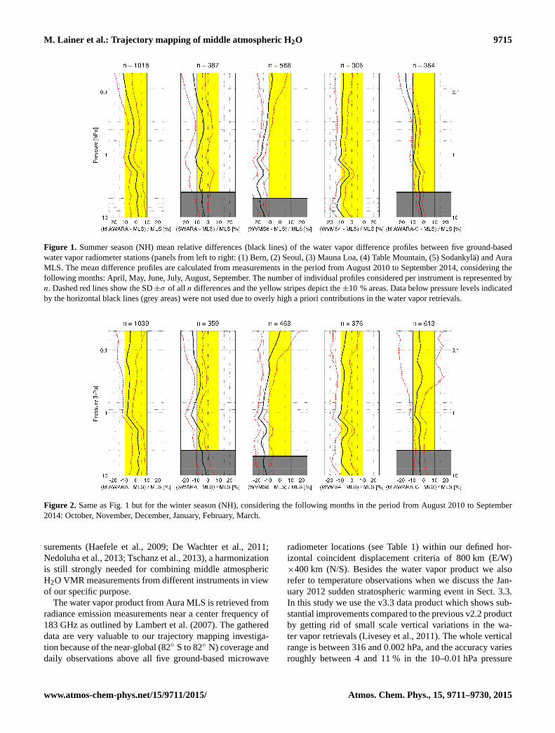
Figure 1. Summer season (NH) mean relative differences (black lines) of the water vapor difference profiles between five ground-based
water vapor radiometer stations (panels from left to right: (1) Bern, (2) Seoul, (3) Mauna Loa, (4) Table Mountain, (5) Sodankylä) and Aura
MLS. The mean difference profiles are calculated from measurements in the period from August 2010 to September 2014, considering the
following months: April, May, June, July, August, September. The number of individual profiles considered per instrument is represented by
n. Dashed red lines show the SD±σ of all n differences and the yellow stripes depict the ±10 % areas. Data below pressure levels indicated
by the horizontal black lines (grey areas) were not used due to overly high a priori contributions in the water vapor retrievals.
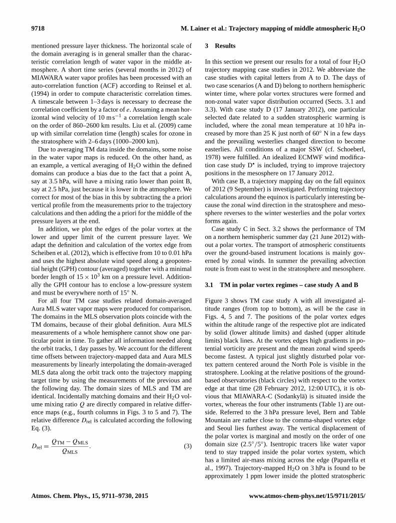
Figure 2. Same as Fig. 1 but for the winter season (NH), considering the following months in the period from August 2010 to September
2014: October, November, December, January, February, March.
surements (Haefele et al., 2009; De Wachter et al., 2011;
Nedoluha et al., 2013; Tschanz et al., 2013), a harmonization
is still strongly needed for combining middle atmospheric
H2O VMR measurements from different instruments in view
of our specific purpose.
The water vapor product from Aura MLS is retrieved from
radiance emission measurements near a center frequency of
183 GHz as outlined by Lambert et al. (2007). The gathered
data are very valuable to our trajectory mapping investiga-
tion because of the near-global (82◦ S to 82◦ N) coverage and
daily observations above all five ground-based microwave
radiometer locations (see Table 1) within our defined hor-
izontal coincident displacement criteria of 800 km (E/W)
×400 km (N/S). Besides the water vapor product we also
refer to temperature observations when we discuss the Jan-
uary 2012 sudden stratospheric warming event in Sect. 3.3.
In this study we use the v3.3 data product which shows sub-
stantial improvements compared to the previous v2.2 product
by getting rid of small scale vertical variations in the wa-
ter vapor retrievals (Livesey et al., 2011). The whole vertical
range is between 316 and 0.002 hPa, and the accuracy varies
roughly between 4 and 11 % in the 10–0.01 hPa pressure
www.atmos-chem-phys.net/15/9711/2015/ Atmos. Chem. Phys., 15, 9711–9730, 2015

9716 M. Lainer et al.: Trajectory mapping of middle atmospheric H2O
regime. A 3.2 to 10 km vertical resolution again in-between
10–0.01 hPa goes along with a spatial wide horizontal res-
olution in the range of 300 to 680 km. We use MLS data if
according to the data quality documentation (Livesey et al.,
2011) quality thresholds are preserved within the addressed
vertical range.
The double differencing method is a useful technique in
the case of a two-instrument network to obtain the bias be-
tween instruments by making use of one traveling satellite,
which observes the same air columns above the ground-
based observation sites. A larger network, such as ours, re-
quires a different strategy. Mean relative difference profiles
are calculated for every single ground-based instrument to
Aura MLS in a quasi-seasonal (6-month periods) manner to
take the bias into account. All individual profiles are linearly
interpolated in logarithmic pressure to cover the same verti-
cal extent (10–0.05 hPa) with the identical number of 1000
grid points, which serve later as trajectory starting points.
The mean relative difference profiles (Figs. 1 and 2) re-
veal that nearly all relative H2O deviations are within±15 %.
An exception is WVMS6 located in Hawaii with deviations
exceeding 15 %. As the yellow bands indicate, the instru-
ments at Bern, Seoul, Table Mountain and Sodankylä have
biases of less than 10 % to MLS in most of the regarded al-
titude ranges. During both the April to September and the
October to March periods, the mean difference water vapor
profiles of all measurement sites show an abrupt increase
of 5–10 % difference to MLS from around 2 to 1 hPa. De-
spite small variations in the seasonal behavior of the SD
(standard deviation) σ the profile structures stay compara-
ble. The largest uncertainty (σ ≈ 20 %) in the mean differ-
ence can be assigned to MIAWARA-C observations above
the polar winter stratopause. Several hundreds of profiles are
processed in the time period from August 2010 until Septem-
ber 2014 to calculate the mean difference H2O profiles, serv-
ing as height-dependent correction factors to harmonize the
trajectory-mapped H2O VMR values during the synthesis of
hemispheric maps (see Sect. 2.4).
In summary, all averaged ground-based measurements of
the five instrument locations result in a negative bias to Aura
MLS throughout all of the studied altitudes; i.e., the water
vapor mixing ratio measured by MLS is consistently higher
than that measured by ground-based instruments.
2.3 The trajectory model
Numerical trajectory simulations in the middle atmosphere
were performed with LAGRANTO (Wernli and Davies,
1997), a software tool consisting of UNIX shell scripts and
FORTRAN programs to analyze Lagrangian aspects of at-
mospheric phenomena. The program requires a time series
of 3-dimensional wind fields in NetCDF files. Possible er-
ror sources are interpolation steps and uncertainties in me-
teorological input data. Interpolation errors develop when
the model wind field from the model time and grid resolu-
tion is interpolated to an actual trajectory location in the 4-
dimensional continuum. With respect to the true atmospheric
state, errors will remain in the initial model conditions, lim-
iting the accuracy of the wind fields.
The 3-dimensional wind vector data are from the European
Centre for Medium-Range Weather Forecasts (ECMWF). A
daily model run (cycle 37R3 – T1279) provides meteorologi-
cal data sets on a 6 hourly spaced time interval from midnight
to midnight. The operational model analysis provides 91 ver-
tical model levels from the surface up to 0.02 hPa. A regular
latitude/longitude grid with a resolution of 1.125◦×1.125◦ is
used for the horizontal plane. Scheiben et al. (2012) created
middle atmospheric H2O trajectory maps of synoptic scale
also with 6 hourly ECMWF data, but at a higher horizontal
resolution of 0.5◦× 0.5◦. Our results suggest that the hori-
zontal model resolution is not a key factor and more accurate
trajectory maps can be produced with a lower LAT/LON res-
olution, even during dynamical extreme events. In general,
errors connected to wind field interpolations are of signifi-
cant relevance. According to Stohl et al. (1995) errors (e.g.,
gridded ECMWF model variables) related to spatial interpo-
lations are much smaller than those related to temporal inter-
polations, which are the primary limiting factor of the accu-
racy of trajectories. The interpolation of the horizontal wind
components is less error-prone than for the vertical motion
w. Stohl et al. (1995) described in their study that a doubling
of the temporal model resolution from 3 to 6 h can result in
up to 40 % mean relative interpolation errors of the vertical
wind component.
Most modern trajectory models use the second-order iter-
ative Petterssen scheme (Petterssen, 1940) in their dynamical
core for solving the trajectory (Eq. 1).
Dx
Dt= u(x, t). (1)
The Petterssen scheme (Eq. 2) has a truncation (numerical
dispersion) error proportional to1t2 where1t is the numer-
ical time step. This error occurs, when higher order terms in
the Taylor expansion are neglected. In Eq. (2) x0 describes
the initial position vector, whereas x1, xn correspond to the
positions after 1 respectively n iteration steps.
x1 = x0+1t ·u(x0, t)
xn = x0+1
21t[u(x0, t)+u(xn−1, t +1t)]. (2)
The external velocity field u(x, t) and a second-order semi-
implicit discretization in time and space are needed to com-
pute the future trajectory position. If the Courant–Friedrichs–
Lewy (CFL) criterion (c = u ·1t/1x < 1) is fulfilled, the
computed solution is numerically convergent. Obviously, the
Courant number c depends on the numerical time step 1t
and the wind field variable u. Earlier simulations performed
by Scheiben et al. (2012) revealed that a time step of around
300 s is short enough for calculations with the ECMWF op-
erational data set. There, observations of two ground-based
Atmos. Chem. Phys., 15, 9711–9730, 2015 www.atmos-chem-phys.net/15/9711/2015/

M. Lainer et al.: Trajectory mapping of middle atmospheric H2O 9717
water vapor microwave radiometers were used for trajectory
mapping and it was possible to find the approximate loca-
tion and extension of the stratospheric polar vortex with the
obtained H2O distribution. But irregularities in the measure-
ments and a sparsely distributed observation network could
not match the quality of synoptic maps from satellite obser-
vations.
The applied trajectory mapping method uses the follow-
ing assumption. It is assumed that an air parcel’s water va-
por volume mixing ratio stays constant while moving along
a 3-dimensional 10-day trajectory. Hence, turbulent mixing,
photolysis, chemical reactions and phase changes of H2O are
not taken into account. Schoeberl and Sparling (1995) as well
as Morris et al. (1995) already showed with trajectory studies
that a time period of 10 days for forward or backward trajec-
tories is a reasonable timescale in the stratosphere. We will
make use of 10-day trajectories up to 0.05 hPa.
2.4 Trajectory mapping – synthesis of hemispheric
H2O maps
LAGRANTO initializes trajectory calculations with starting
points of an air parcel in a latitude, longitude and pressure
level coordinate system. To generate synoptic maps with tra-
jectory mapping, the definition of a pressure layer with a cer-
tain thickness 1p is required. In order to increase the num-
ber of trajectory arrival points from instrument observations
(trajectory starting points) inside a defined pressure layer,
different implementations such as increasing the TM pres-
sure layer thickness, the number of vertical trajectory start-
ing points with interpolation or an extended instrument net-
work might be considered. Keeping in mind that a maximal
vertical measurement resolution of ∼ 10 km is realistic, the
number of vertical starting points can only be enlarged by
interpolation of the water vapor profiles. The largest uncer-
tainties during the LAGRANTO calculations are likely aris-
ing from the interpolation of the vertical wind component. It
is important that the starting points of the trajectory calcula-
tions in LAGRANTO are within the ECMWF vertical model
grid (91 levels). Otherwise the interpolations to the starting
point positions are impossible. Horizontal interpolations of
the ECMWF wind field data to the actual trajectory positions
are bilinear; vertical ones linear with pressure and time inter-
polations are also performed linearly.
The water vapor profiles of the instrument network are in-
terpolated to a pressure grid with a logarithmic equispaced
subdivision of 1000 pressure levels between 10–0.05 hPa.
This is equal to a ∼ 37 m vertical grid point spacing. Ac-
cording to instrument features and retrieval versions differ-
ent altitude data cut-off limits in the stratosphere are used as
described in Sect. 2.1 and illustrated with the bias correction
plots of Figs. 1 and 2. The interpolated volume mixing ratios
on the grid points are used to create raw trajectory maps. Al-
together 20 days of water vapor profile measurements from
each instrument are taken. As the temporal resolution varies
between 12 and 24 h, one or two profiles per day are obtained
accordingly. A mean time is assigned to each profile, which
results in a H2O profile time series. Because the wind field
data of the ECMWF model that go into LAGRANTO have
temporal resolution of 6 h, we further temporally interpolate
the prior pressure interpolated profile time series of every sin-
gle radiometer onto the time grid of the ECMWF model.
Now trajectories can be calculated every 6 h starting from
every grid point of the processed profiles. For 20 days and
with four profiles per day plus the initial profile on the TM
target time (4 · 20)+ 1= 81 profiles are created over one
ground-based instrument location. If measurement gaps ex-
tend over more than 96 h the mixing ratios of the correspond-
ing interpolated water vapor profiles are disregarded. The re-
maining data are needed to synthesize a trajectory map at
the center of the 20-day time period of considered measure-
ments. Forward trajectories are calculated for the first 40 wa-
ter vapor profiles of each measurement site and the corre-
sponding backward trajectories for the last 40 profiles. The
profile number 41 is already at the right position in time for
the trajectory map. If all trajectories are summed for a 20-
day period and five ground-based stations, we count 4× 10⁵
trajectories.
The volume mixing ratios from the grid points of the pro-
files belonging to the trajectory start points were assigned to
the new calculated trajectory end points, assuming that the
H2O mixing ratio stays constant. While we are calculating
3-dimensional paths through the atmosphere, the trajectory
end points can rise or sink in altitude. A simple filtering is
done to separate out the mixing ratios of points within the
different defined pressure layers (12–8, 3.5–2.5, 1.3–0.7 and
0.13–0.07 hPa) in order to get a simple raw TM map, consist-
ing of single points in 3-dimensional space, at 12:00 UTC. A
problem with a thick pressure layer can be that a less homo-
geneous trajectory map is produced if large vertical gradients
in H2O exist. The trajectory origin of the single points can be
outside the previous defined pressure layers due to rising or
descending trajectories. Later in Sect. 3 we only refer to the
middle of the pressure layers (10, 3, 1 and 0.1 hPa). The cho-
sen layers ensure that at least one MLS measurement on the
native vertical resolution is situated at or close to the middle
of a layer.
On the basis of raw trajectory maps alone, a quantita-
tive verification to other measurements would be difficult.
With the idea of uniquely defined 3-dimensional domains,
where the trajectory-mapped H2O VMR data are averaged,
a proper solution for following verifications was found. De-
pending on whether domains are in the stratosphere or meso-
sphere, the horizontal expansion varies from 2.5◦× 2.5◦ to
5◦×5◦ (LAT×LON) in the domain-averaged TM maps. With
a doubling of the horizontal domain-averaging size at the
stratopause region and above, we accounted for the altitude
increasing uncertainty of middle atmospheric ECMWF wind
fields by an increased blurring of trajectory endpoint posi-
tions. The vertical extent is in agreement with the previous
www.atmos-chem-phys.net/15/9711/2015/ Atmos. Chem. Phys., 15, 9711–9730, 2015
9718 M. Lainer et al.: Trajectory mapping of middle atmospheric H2O
mentioned pressure layer thickness. The horizontal scale of
the domain averaging is in general smaller than the charac-
teristic correlation length of water vapor in the middle at-
mosphere. A short time series (several months in 2012) of
MIAWARA water vapor profiles has been processed with an
auto-correlation function (ACF) according to Reinsel et al.
(1994) in order to compute characteristic correlation times.
A timescale between 1–3 days is necessary to decrease the
correlation coefficient by a factor of e. Assuming a mean hor-
izontal wind velocity of 10 ms−1 a correlation length scale
on the order of 860–2600 km results. Liu et al. (2009) came
up with similar correlation time (length) scales for ozone in
the stratosphere with 2–6 days (1000–2000 km).
Due to averaging TM data inside the domains, some noise
in the water vapor maps is reduced. On the other hand, as
an example, a vertical averaging of H2O within the defined
domains can produce a bias due to the fact that a point A,
say at 3.5 hPa, will have a mixing ratio lower than point B,
say at 2.5 hPa, just because it is lower in the atmosphere. We
correct for most of the bias in this by subtracting the a priori
vertical profile from the measurements prior to the trajectory
calculations and then adding the a priori for the middle of the
pressure layers at the end.
In addition, we plot the edges of the polar vortex at the
lower and upper limit of the current pressure layer. We
adapt the definition and calculation of the vortex edge from
Scheiben et al. (2012), which is effective from 10 to 0.01 hPa
and uses the highest absolute wind speed along a geopoten-
tial height (GPH) contour (averaged) together with a minimal
border length of 15× 103 km on a pressure level. Addition-
ally the GPH contour has to enclose a low-pressure system
and must be everywhere north of 15◦ N.
For all four TM case studies related domain-averaged
Aura MLS water vapor maps were produced for comparison.
The domains in the MLS observation plots coincide with the
TM domains, because of their global definition. Aura MLS
measurements of a whole hemisphere cannot show one par-
ticular point in time. To gather all information needed along
the orbit tracks, 1 day passes by. We account for the different
time offsets between trajectory-mapped data and Aura MLS
measurements by linearly interpolating the domain-averaged
MLS data along the orbit track onto the trajectory mapping
target time by using the measurements of the previous and
the following day. The domain sizes of MLS and TM are
identical. Incidentally matching domains and their H2O vol-
ume mixing ratio Q are directly compared in relative differ-
ence maps (e.g., fourth columns in Figs. 3 to 5 and 7). The
relative difference Drel is calculated according the following
Eq. (3).
Drel =QTM−QMLS
QMLS
. (3)
3 Results
In this section we present our results for a total of four H2O
trajectory mapping case studies in 2012. We abbreviate the
case studies with capital letters from A to D. The days of
two case scenarios (A and D) belong to northern hemispheric
winter time, where polar vortex structures were formed and
non-zonal water vapor distribution occurred (Sects. 3.1 and
3.3). With case study D (17 January 2012), one particular
selected date related to a sudden stratospheric warming is
included, where the zonal mean temperature at 10 hPa in-
creased by more than 25 K just north of 60◦ N in a few days
and the prevailing westerlies changed direction to become
easterlies. All conditions of a major SSW (cf. Schoeberl,
1978) were fulfilled. An idealized ECMWF wind modifica-
tion case study D? is included, trying to improve trajectory
positions in the mesosphere on 17 January 2012.
With case B, a trajectory mapping day on the fall equinox
of 2012 (9 September) is investigated. Performing trajectory
calculations around the equinox is particularly interesting be-
cause the zonal wind direction in the stratosphere and meso-
sphere reverses to the winter westerlies and the polar vortex
forms again.
Case study C in Sect. 3.2 shows the performance of TM
on a northern hemispheric summer day (21 June 2012) with-
out a polar vortex. The transport of atmospheric constituents
over the ground-based instrument locations is mainly gov-
erned by zonal winds. In summer the prevailing advection
route is from east to west in the stratosphere and mesosphere.
3.1 TM in polar vortex regimes – case study A and B
Figure 3 shows TM case study A with all investigated al-
titude ranges (from top to bottom), as will be the case in
Figs. 4, 5 and 7. The positions of the polar vortex edges
within the altitude range of the respective plot are indicated
by solid (lower altitude limits) and dashed (upper altitude
limits) black lines. At the vortex edges high gradients in po-
tential vorticity are present and the mean zonal wind speeds
become fastest. A typical just slightly disturbed polar vor-
tex pattern centered around the North Pole is visible in the
stratosphere. Looking at the relative positions of the ground-
based observatories (black circles) with respect to the vortex
edge at that time (28 February 2012, 12:00 UTC), it is ob-
vious that MIAWARA-C (Sodankylä) is situated inside the
vortex, whereas the four other instruments (Table 1) are out-
side. Referred to the 3 hPa pressure level, Bern and Table
Mountain are rather close to the comma-shaped vortex edge
and Seoul lies furthest away. The vertical displacement of
the polar vortex is marginal and mostly on the order of one
domain size (2.5◦/5◦). Isentropic tracers like water vapor
tend to stay trapped inside the polar vortex system, which
has a limited air-mass mixing across the edge (Paparella et
al., 1997). Trajectory-mapped H2O on 3 hPa is found to be
approximately 1 ppm lower inside the plotted stratospheric
Atmos. Chem. Phys., 15, 9711–9730, 2015 www.atmos-chem-phys.net/15/9711/2015/
M. Lainer et al.: Trajectory mapping of middle atmospheric H2O 9719
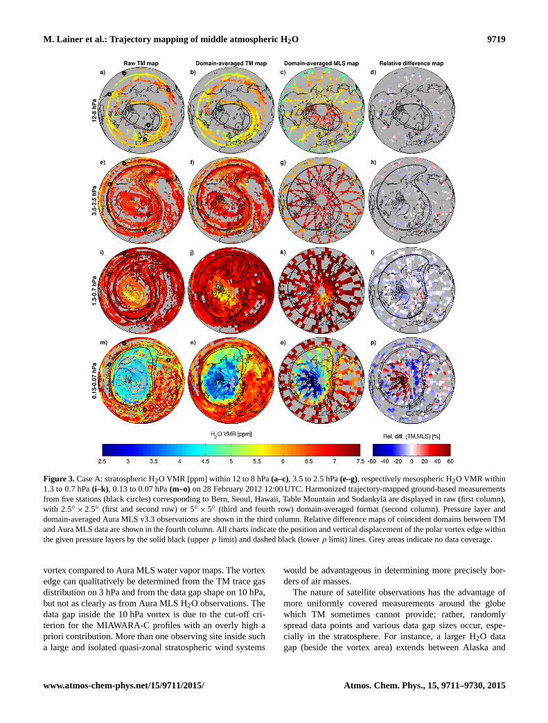
Figure 3. Case A: stratospheric H2O VMR [ppm] within 12 to 8 hPa (a–c), 3.5 to 2.5 hPa (e–g), respectively mesospheric H2O VMR within
1.3 to 0.7 hPa (i–k), 0.13 to 0.07 hPa (m–o) on 28 February 2012 12:00 UTC. Harmonized trajectory-mapped ground-based measurements
from five stations (black circles) corresponding to Bern, Seoul, Hawaii, Table Mountain and Sodankylä are displayed in raw (first column),
with 2.5◦× 2.5◦ (first and second row) or 5◦× 5◦ (third and fourth row) domain-averaged format (second column). Pressure layer and
domain-averaged Aura MLS v3.3 observations are shown in the third column. Relative difference maps of coincident domains between TM
and Aura MLS data are shown in the fourth column. All charts indicate the position and vertical displacement of the polar vortex edge within
the given pressure layers by the solid black (upper p limit) and dashed black (lower p limit) lines. Grey areas indicate no data coverage.
vortex compared to Aura MLS water vapor maps. The vortex
edge can qualitatively be determined from the TM trace gas
distribution on 3 hPa and from the data gap shape on 10 hPa,
but not as clearly as from Aura MLS H2O observations. The
data gap inside the 10 hPa vortex is due to the cut-off cri-
terion for the MIAWARA-C profiles with an overly high a
priori contribution. More than one observing site inside such
a large and isolated quasi-zonal stratospheric wind systems
would be advantageous in determining more precisely bor-
ders of air masses.
The nature of satellite observations has the advantage of
more uniformly covered measurements around the globe
which TM sometimes cannot provide; rather, randomly
spread data points and various data gap sizes occur, espe-
cially in the stratosphere. For instance, a larger H2O data
gap (beside the vortex area) extends between Alaska and
www.atmos-chem-phys.net/15/9711/2015/ Atmos. Chem. Phys., 15, 9711–9730, 2015

9720 M. Lainer et al.: Trajectory mapping of middle atmospheric H2O
Figure 4. Case B: same as Fig. 3, except for 22 September 2012, 12:00 UTC close to the fall equinox.
China just south of the stratospheric vortex as Fig. 3b re-
veals. The coverage over Europe is in contrast quite good.
With increasing altitude, the water vapor observations from
Sodankylä almost reach the inner mesospheric vortex edge in
case A (28 February 2012), but data from MIAWARA-C still
mainly contribute for the part of the map which is framed
by the vortex. Contrarily in the two higher altitude regions
(Fig. 3j and n) the hemispherical coverage of water vapor
data is much better in the synthesized domain-averaged TM
map than in the Aura MLS map (Fig. 3k and o). A main ad-
vantage of the synthesized water vapor maps is a temporal
coherent data set without any post-processing, covering over
95 % of the Northern Hemisphere on the 1 and 0.1 hPa pres-
sure level. The area covered by TM data is remarkable and
similar to that in the TM case scenario B for the 0.1 hPa and
D for the 1 and 0.1 hPa pressure level (see Figs. 4n and 7j
and n). The minimum H2O mixing ratios inside the 1 hPa
(stratopause) and 0.1 hPa vortices coincide very well. An
eastward shift in the position of the lowest VMR domains is
apparent between the Aura MLS and TM water vapor maps
for the stratopause region. A mesospheric vortex position at
0.1 hPa can be seen in both TM and direct satellite observa-
tion techniques (Fig. 3n and o). A perceptible difference be-
tween Fig. 3m and n in areas with low water vapor is likely
due to the applied correction for vertical averaging in the do-
main TM map (cf. Sect. 2.4).
TM case B is represented in Fig. 4. The trajectory mapping
target time was 22 September 2012, 12:00 UTC, the second
Atmos. Chem. Phys., 15, 9711–9730, 2015 www.atmos-chem-phys.net/15/9711/2015/

M. Lainer et al.: Trajectory mapping of middle atmospheric H2O 9721
Figure 5. Case C: same as Fig. 3, except for 21 June 2012, 12:00 UTC close to the June solstice.
day of equinox in the year 2012. A rapid increase in plane-
tary wave mode 1 usually occurs near the fall equinox in the
Northern Hemisphere, and their propagated and transferred
momentum drives the zonal west wind circulation in the
middle atmosphere (Liu et al., 2001). Regarding the consid-
ered pressure layers, inside-the-vortex measurements from
the ground-based instrument network were always available
on the TM target date, if the measurement response down
to 10 hPa was high enough. Nevertheless there is the pos-
sibility that subsiding air from higher altitudes can provide
TM data down to lower altitudes. The polar vortex edge de-
tection algorithm worked for the equinox scenario (B) and
the reformed vortex after the summer season. For the meso-
spheric vortex (see Fig. 4m), a large vertical gradient of the
edge is evident, where a 3-dimensional interpretation would
be cone-shaped.
The hemispheric coverage of the TM H2O VMR data of
case study B in the stratosphere and on stratopause level
(Fig. 4a, e and i) is not as good as for the previous case
study A, but similar for the 0.1 hPa pressure level. Some
larger measurement gaps between 12 September and 2 Octo-
ber 2012 in the Table Mountain and Hawaii data lead to a re-
duced number of the TM values of water vapor in case B. The
visual impression of the comparison between Fig. 4f and g
gives the result that TM can reproduce the H2O VMR within
a few percent of relative difference along the inner black vor-
tex contours, as the relative difference maps to Aura MLS ob-
servations (Fig. 4h) prove. Horizontal meridional H2O VMR
www.atmos-chem-phys.net/15/9711/2015/ Atmos. Chem. Phys., 15, 9711–9730, 2015

9722 M. Lainer et al.: Trajectory mapping of middle atmospheric H2OLatitude[deg]
Aura MLS v3.3 zonal mean temperature at 10 hPa
Jan12 Feb12 Mar120
15
30
45
60
75
90
T[K]
190
200
210
220
230
240D A
Latitu
de [deg]
ECMWF zonal mean zonal wind at 10 hPa
Jan12 Feb12 Mar120
15
30
45
60
75
90
u [m
/s]
−50
0
50
Figure 6. Northern hemispheric Aura MLS v3.3 zonal mean temperature in [K] (upper pannel) and ECMWF
zonal mean zonal wind in [m s−1] for the 10hPa pressure level. The time period extends from mid-December
2011 to mid-March 2012. The left dashed black line indicates the date of TM case D and the right one TM case
A.
29
Figure 6. Northern hemispheric Aura MLS v3.3 zonal mean tem-
perature in [K] (upper panel) and ECMWF zonal mean zonal wind
in [ms−1] for the 10 hPa pressure level. The time period extends
from mid-December 2011 to mid-March 2012. The left dashed
black line indicates the date of TM case D and the right one TM
case A.
gradients match well between Aura MLS and TM maps for
the 3 and 1 hPa altitude. At 0.1 hPa trajectory-mapped wa-
ter vapor tends to be too low on the order of 5–10 %, as
is obvious in Fig. 4p, where bluish domains are prevalent.
In general, horizontal gradients in water vapor were found
to be higher in the stratosphere than in the mesosphere near
equinox.
To sum up so far, Aura MLS water vapor observations
show a quite good and widespread agreement over the an-
alyzed pressure levels of case scenarios A and B in relation
to the generated TM maps, which have more noise (variabil-
ity between neighboring domains) in water vapor. Reducing
the noise of TM data without smoothing algorithms is diffi-
cult. More accurate wind field data with a higher temporal
resolution could improve the TM quality in the sense of de-
creasing noise in the horizontal water vapor distribution and
trajectory position errors.
3.2 TM in a non-polar vortex regime – case study C
The prevailing wind direction in the middle atmosphere re-
verses seasonally, in winter the winds are mainly eastward
and in summer westward. Enhanced gravity wave activity
during NH winter leads to a deposition of angular momen-
tum in the middle atmosphere and decelerates the zonal flow.
Meridional transport of atmospheric constituents in summer
is limited, because of missing wave-induced forces driving
north–south circulations (Holton and Alexander, 2000). As
a consequence, trace constituents in the NH summer strato-
and mesosphere become fairly evenly distributed around lat-
itudinal bands within weeks because there are no dynamical
barriers to atmospheric transport as provided by the winter-
time stratospheric polar vortex. Circle like structures in the
TM water vapor maps of Fig. 5, close to the June solstice, ex-
emplify the situation. With only five measurement locations,
whereof two (Seoul and Table Mountain) are almost at the
same latitude, the hemispheric coverage compared to Aura
MLS is poor. If we intend to reduce the water vapor gaps in
summer time, ground-based observations of more latitudes
from tropical to polar regions would be necessary. Stations
located at various longitudes are much more important in the
winter than in the summer period. A spatial interpolation of
H2O in environments where the horizontal gradient is small
(Fig. 5c and g) or even absent (Fig. 5k) could be taken into
consideration to fill in the gaps. For filling in data gaps in
the satellite observational record, analysis or reanalysis data
from e.g., ECMWF could be used. Thus an increased num-
ber of possible comparison domains would be created. This
concept has not been implemented, because the accuracy of
moisture fields in ECMWF model could be problematic in
the upper atmosphere. Some studies (e.g., Feist et al., 2007)
found that the ECMWF model produces an unrealistically
moist mesosphere, which is not present in the MLS observa-
tions. And more importantly, there is no stratospheric H2O
data assimilated in the ECMWF integrated forecasting sys-
tem (IFS), and we think that using the model data above the
troposphere is not an alternative regarding the TM map vali-
dation.
In the stratosphere of case study C the difference between
the highest (high LAT) and lowest (low LAT) mixing ratios is
on the order of 1 ppm, what is confirmed by TM (see Fig. 5b
and f). The 10 hPa trajectory map shows that WVMS6 and
MIAWARA-C instruments are not able to provide valuable
scientific information for this pressure layer (12–8 hPa).
The H2O VMR distribution at the 1 and 0.1 hPa level is
quite uniform and reaches values between 7 and 8 ppm as 3
months later in the case of scenario B. With increasing alti-
tude, the water vapor coverage over the Northern Hemisphere
is found to increase in the TM plots (Fig. 5a, e, i and m). The
short-scale H2O variation (noise) is obvious in the Aura MLS
map in Fig. 5o.
3.3 Performance during the January 2012 SSW – case
study D
We restrict the temporal description of the major SSW of Jan-
uary 2012 to Aura MLS zonal mean temperature measure-
ments and ECMWF zonal mean zonal winds on the 10 hPa
pressure surface. Figure 6 shows a strong negative tempera-
ture gradient north of 40◦ N right before the end of Decem-
ber 2011 in connection with the stratospheric polar vortex.
At the beginning of January 2012, the temperature gradient
started to weaken and reversed near the middle of the month.
The increase in zonal mean temperature in the polar strato-
sphere is about 25 K during 1 week. In the same period of
Atmos. Chem. Phys., 15, 9711–9730, 2015 www.atmos-chem-phys.net/15/9711/2015/

M. Lainer et al.: Trajectory mapping of middle atmospheric H2O 9723
Figure 7. Case D: same as Fig. 3, except for 17 January 2012, 12:00 UTC close to the maximum temperature increase at 10 hPa during a
major SSW in the Northern Hemisphere.
time, the ECMWF operational analysis of the mean zonal
wind component shows a reversal from westerly to easterly
winds. Compared to the January 2010 major SSW, described
in Scheiben et al. (2012), the temperature increase in this case
was not so abrupt and also the duration of the easterlies at
10 hPa did not persist as long. After the SSW the tempera-
tures decreased again in the stratosphere north of 45◦ N, but
did not reach as low values as in December 2011 (∼ 205 K
compared to 190 K) owing to a less intense reformation of
the polar vortex.
Case D (Fig. 7) occurs near the time of the maximum tem-
perature observed on 10 hPa during the 2012 SSW. The dis-
tortion and weakening of the vortex is a difficult situation for
applying trajectory mapping. By comparing the position of
the vortex edge contours between 10 and 3 hPa, big differ-
ences in size and position can be found. The mean vortex
edge horizontal wind velocities decline by almost 10 ms−1
when going up in altitude from 10 to 3 hPa. Usually, in an
undisturbed and stable circulation environment in NH win-
ters the opposite (increasing wind speeds with altitude) is
typical in the stratosphere. Regarding the trajectory map and
MLS H2O footprints on the 10 hPa reference layer a good
match is found (cf. Fig. 7b–d as well as f–h).
Trajectory mapping of water vapor in the mesosphere dur-
ing a SSW provides synoptic maps of slightly reduced qual-
ity and higher errors (Fig. 7n and p). However in this instance
www.atmos-chem-phys.net/15/9711/2015/ Atmos. Chem. Phys., 15, 9711–9730, 2015

9724 M. Lainer et al.: Trajectory mapping of middle atmospheric H2O
it is found to work even better than in case A with a stable
polar vortex environment. To perfectly match the noisy Aura
MLS map (Fig. 7o) is by chance very unlikely. The correla-
tion between these differences (TM−MLS) and photolytic
or chemical processes, which are entirely neglected, is not
evaluated. We note that the ECMWF winds become increas-
ingly uncertain with increasing altitude, and may contribute
significantly to the observed differences between MLS and
the ground-based radiometers.
3.4 Modification of ECMWF mesospheric wind
velocities – case study D?
Additionally we want to briefly describe a performed sen-
sitivity study with the ECMWF wind field data, that might
improve mesospheric trajectory positions. Based on mea-
surements from the ground-based microwave Doppler wind
radiometer WIRA (Rüfenacht et al., 2014) during different
campaigns, which suggests that ECMWF wind components
(u, v and w) are overestimated in the mesosphere (above
1 hPa) by the model, a constant downscaling of u, v and
w by 30 % on all model grid points above 1 hPa has been
performed and new trajectories were calculated with LA-
GRANTO for the SSW case study D to synthesize new
H2O trajectory maps (case study D?). Compared to the Aura
MLS water vapor maps a non-significant improvement in the
0.13–0.07 hPa pressure layer could be detected (cf. last two
columns in Table 2). Less than 4 % more coincident relative
comparison domains display a difference of up to ±10 % to
Aura MLS H2O VMR domains. From this point of view it is
not possible to cross-check and prove whether the ECMWF
winds in the mesosphere are indeed too high. An assessment
for effects of potential error sources in the TM analysis, such
as wind errors, chemical reactions or a removal of water va-
por by phase transitions (e.g., mesospheric clouds), is pre-
sented in Sect. 3.6.
3.5 Validation and statistical analysis with MLS
In addition to the relative difference maps shown before, his-
tograms are plotted for every individual case study to illus-
trate the number of matching domains corresponding to devi-
ation bins with a width of 5 % in the pressure layers. The his-
tograms and relative difference maps are used for a statistical
analysis and validation. Table 2 further summarizes the per-
centage of H2O VMR domains within 10, respectively 20 %
relative difference (Drel, see Eq. 3) between TM and Aura
MLS results. Further, percentages corresponding to the TM
performance without instrument bias corrections are given.
The relative differences to Aura MLS in the domain ar-
eas do not exceed 20 % in most cases and altitude regions.
Regarding the whole number of domains per map, only a
few outliers with deviations Drel > | ± 20| % are present at
pressure levels below 0.1 hPa as confirmed in the histogram
charts (Fig. 8). The deviation bins with the maximum number
of relative difference domains (peak of Gaussian curve) are
centered around the zero percent line (perfect coincidence),
except for the lowest altitude in case study B and D where the
TM domains show either too high (case B) or too low (case
D) H2O VMR values and for the highest altitude in all cases
where overly low mixing ratios from TM dominate.
Table 2 underlines the good results of the TM approach
with respect to Aura MLS observations. Referred to the bias
corrected row values of case A and B in the stratosphere
and stratopause level (1 hPa), between 98.4 and 100 % of
the compared domains have a difference of less than ±20 %.
At least around half of all domains from the investigated
difference maps in Figs. 3 and 4d and h are indeed within
±10 %. By ignoring case B with its small statistical sig-
nificance, slightly over 82 % (83 %) of the domains agree
within ±10 % in case A at 10 hPa (3 hPa). Within the meso-
spheric vortices a significant number of domains show that
TM resulted in too high H2O VMR values (reddish colors in
the February polar vortex case study in Fig. 3p). Inside the
equinox polar vortex this feature is not present. In the his-
togram of case A (0.1 hPa) roughly 15 domains exist with a
difference of 95–100 %, located in the vortex over Greenland
and westwards thereof. While the Gaussian center line still
lies close to the zero percent line (green), the shape of the
histogram spreads. The homogeneous distributed water va-
por in case study B at 0.1 hPa with values around 7 to 8 ppm
(Fig. 4o) is better confirmed by TM than in the previous sit-
uation. In numbers we now count 46.1 % (case study A) and
80 % (case study B) of the domains to be within the ±10 %
deviation limit but at least 75.7 and 99.4 % are within the
doubled deviation threshold of 20 %.
Regarding TM case study C (21 June 2012) close to the
June solstice event, the number of coincident TM and MLS
domains is reduced on the investigated stratospheric pressure
levels owing to zonal circulation patterns compared to case
study A or D. Throughout the middle atmosphere, all rela-
tive difference domains from high to low latitude bands show
only light blue to light red colors (Fig. 5d, h, l and p). The
deviations in H2O VMR are tiny, the histograms are always
narrow. More than 350 (200) 5◦× 5◦ domains are within ±5
% at 1 hPa (3 hPa) and nearly all compared areas show less
than 20 % relative difference (cf. Table 2) on all four altitude
levels.
Next we show the agreement of TM results with MLS ob-
servations in case study D (17 January 2012), the SSW event.
As it is affirmed by Fig. 7, the prolonged shape of the vortex
is very well represented by the applied trajectory mapping
method at the lowest investigated altitude. Less than 2 % of
the compared domains deviate more than 20 % in relative
difference. Examining the variations in H2O VMR of the in-
ner parts of the 3 hPa vortex on 17 January 2012, the outcome
has to be evaluated positively with a majority of domains that
satisfy the 10 % relative difference quality criterion (Figs. 7h
and 8). The more or less uniform H2O distribution of 7–
7.5 ppm in MLS (Fig. 7k) could be displayed correctly by
Atmos. Chem. Phys., 15, 9711–9730, 2015 www.atmos-chem-phys.net/15/9711/2015/

M. Lainer et al.: Trajectory mapping of middle atmospheric H2O 9725
Figure 8. Pressure layer corresponding histograms of TM case study A (28 February 2012, first column), B (22 September 2012, second
column), C (21 June 2012, third column) and D (17 January 2012, fourth column). The number of relative difference (TM−MLS) domains
in a certain deviation bin of a width of 5 % between TM and Aura MLS solution is shown. From top to bottom, the pressure layers are 12–8,
3.5–2.5, 1.3–0.7 and 0.13–0.07 hPa. Vertical green lines indicate zero deviation.
TM (Fig. 7j). There, the relative differences to MLS never
exceed 20 %. At 0.1 hPa the water vapor VMR underesti-
mation by TM is reduced compared to case A at the same
altitude. More than 53 % (89 %) of the compared domains
stay within a relative difference of 10 % (20 %). In the mean,
TM domains revealed low mixing ratios relative to MLS in
the mesospheric pressure layer as the leftward shifted peak
of the histogram reveals.
Summarizing cases A to D, very good agreement between
TM- and MLS-derived water vapor maps was found at the
stratopause level (1 hPa∼ 48 km). All TM domains for case
B, C and D deviate less than 20 % from MLS (see Table 2)
and only a tiny percentage of 0.2 % show larger relative dif-
ferences in case A. Of course histograms show tight bounds
and the full widths at half maxima are small (Fig. 8). We
assume that low planetary wave activity in the upper strato-
sphere around the selected TM dates was accountable for the
low meridional gradients in water vapor in this altitude re-
gion and hence simplified the TM method to work well.
3.6 Error estimation of TM approach
In this section, the strategy and outcome of the investigation
to estimate the error and limitation of the trajectory map-
ping (TM) approach is briefly summarized. In a first step
Aura MLS profiles are taken, located near the five ground-
based observation sites. The chosen criterion for spatial coin-
cident of the satellite measurements is 600× 300 km around
www.atmos-chem-phys.net/15/9711/2015/ Atmos. Chem. Phys., 15, 9711–9730, 2015

9726 M. Lainer et al.: Trajectory mapping of middle atmospheric H2O
Table 2. The percentage of coincident domains in which the H2O from TM and Aura MLS observations agree within 10 (20) % in each
pressure layer. All four studied TM scenarios (A–D) with applied bias correction (Y), according to Sect. 2.2, or no correction (N) are shown.
In the last column the percentages regarding the ECMWF sensitivity case study D? (30 % downscaled mesospheric wind velocities for TM)
are given.
TM Case A B C D D?
Date 28 Feb 2012 22 Sep 2012 21 Jun 2012 17 Jan 2012 17 Jan 2012
12–8 hPa (N) 77.6(99.1) 56.9(96.1) 84.9(100) 70.9(93.9) 70.9(93.9)
12–8 hPa (Y) 82.6(100) 64.7(98.0) 89.0(100) 64.0(98.5) 64.0(98.5)
3.5–2.5 hPa (N) 72.5(96.8) 87.0(99.7) 59.2(93.7) 56.4(96.1) 57.9(95.6)
3.5–2.5 hPa (Y) 83.1(98.4) 86.0(99.1) 92.7(99.1) 91.1(99.3) 91.7(99.3)
1.3–0.7 hPa (N) 37.7(94.0) 57.7(99.7) 51.4(99.3) 66.0(99.8) 74.4(99.6)
1.3–0.7 hPa (Y) 87.0(99.8) 99.7(100) 98.6(100) 98.5(100) 98.4(100)
0.13–0.07 hPa (N) 26.0(66.5) 16.3(84.7) 35.1(88.7) 35.1(75.1) 40.0(80.6)
0.13–0.07 hPa (Y) 46.1(75.7) 80.0(99.4) 76.2(99.1) 53.3(89.3) 57.2(89.8)
the ground-based radiometer locations. The 300 km go along
north–south direction, while the 600 km go along east–west
direction. The unequal lengths are due to typical water va-
por gradients, which tend to be much smaller in zonal than
meridional direction. A similar way of data processing has
been applied to the obtained Aura MLS profile time series,
according to Sect. 2.4. It is evident that correction factors
to account for biases are not necessary, since the same in-
strument is used to generate the H2O profiles. The histogram
charts in Fig. 9 show the results of the investigation. These
charts are similar to the ones in Fig. 8 only with additional
tags for the standard deviations ±σ .
For the three pressure layers at lower altitudes (12–8, 3.5–
2.5 and 1.3–0.7 hPa) it is found that deviations from the co-
incident domain comparison never exceed 20 %. Approxi-
mately 2/3 of all domains show less than 10 % deviation.
The errors become significantly higher in the mesosphere
(0.13–0.07 hPa). Estimating the position of the 2/3 value
of the domains in the bar charts, it is now roughly within
∼ 20 % (doubled) in the mesospheric pressure layers. Re-
garding the standard deviation σ , it is clear that the uncer-
tainties of TM are largest in the mesosphere (0.13–0.07 hPa)
of case study A (28 February 2012). It is also noticeable that
TM during the SSW case D (17 January 2012) reveals less
uncertainties (σ is smaller).
4 Summary and discussion
We have generated NH middle atmospheric water vapor
maps from five single water vapor profile measurement sites,
mainly operated in the frame of NDACC, by use of a spa-
tial domain-averaging trajectory mapping technique. For-
ward and backward trajectories were calculated for up to
10 days with LAGRANTO driven by ECMWF operational
analysis wind field data. A total of four TM case-by-case
studies were presented and discussed, belonging to differ-
ent atmospheric circulation patterns and seasons of the year.
Apart from the SSW scenario (D) in January 2012, we dis-
cussed (1) a stable polar vortex case (A) at the end of Febru-
ary, (2) a case near June solstice (C) and (3) a fall equinox
scenario (B). For each case study four pressure layers from
the stratosphere (centered at 10 hPa) to the lower mesosphere
(centered at 0.1 hPa) were analyzed.
Biases between the ground-based instruments have been
corrected using coincident Aura MLS observations during a
defined time period (August 2010 to September 2014). Cal-
culated mean relative difference profiles of H2O served as
correction factors to harmonize the data sets. The improve-
ments of the bias corrected synoptic maps is very pronounced
above the 3 hPa pressure layer compared to the uncorrected
versions (Table 2). At best (case study B, 0.1 hPa), 80 % in-
stead of 16.3 % of the relative difference domains had a bias
of only ±10 %. For the three upper pressure layers of TM
studies A, C and D/D?, the corrections led always to an im-
provement of trajectory-mapped data, referring to the±10 %
as well as to the ±20 % regime. On the 10 and 3 hPa pres-
sure level the applied correction factors led sometimes to a
slight worsening for cases B and D/D?, for instance a loss of
almost 10 % of comparison domains (case D/D? on 10 hPa),
which were associated to the 10 % quality threshold.
The mesospheric polar vortex edge was very well repro-
duced, with the trajectory mapping method by the north–
south gradient in water vapor VMR on 28 February 2012
(Fig. 3n). In the mesosphere, where uncertainties in the 3-
dimensional wind field become larger, leading to trajectory
position errors, the quality of the TM-derived water vapor
distribution is generally reduced, compared to coincident
Aura MLS observations. However, the TM data coverage is
found to be better at higher altitudes such as at the 0.1 hPa
level in the mesosphere. In addition, the assumption of un-
changed mixing ratios along 240 h trajectories might not be
sufficient any more in mesospheric altitudes where photol-
ysis or chemical reactions of water vapor cannot be totally
Atmos. Chem. Phys., 15, 9711–9730, 2015 www.atmos-chem-phys.net/15/9711/2015/
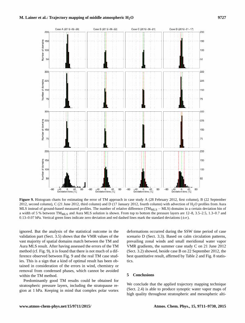
M. Lainer et al.: Trajectory mapping of middle atmospheric H2O 9727
Figure 9. Histogram charts for estimating the error of TM approach in case study A (28 February 2012, first column), B (22 September
2012, second column), C (21 June 2012, third column) and D (17 January 2012, fourth column) with advection of H2O profiles from Aura
MLS instead of ground-based measured profiles. The number of relative difference (TMMLS−MLS) domains in a certain deviation bin of
a width of 5 % between TMMLS and Aura MLS solution is shown. From top to bottom the pressure layers are 12–8, 3.5–2.5, 1.3–0.7 and
0.13–0.07 hPa. Vertical green lines indicate zero deviation and red dashed lines mark the standard deviations (±σ ).
ignored. But the analysis of the statistical outcome in the
validation part (Sect. 3.5) shows that the VMR values of the
vast majority of spatial domains match between the TM and
Aura MLS result. After having assessed the errors of the TM
method (cf. Fig. 9), it is found that there is not much of a dif-
ference observed between Fig. 9 and the real TM case stud-
ies. This is a sign that a kind of optimal result has been ob-
tained in consideration of the errors in wind, chemistry or
removal from condensed phases, which cannot be avoided
within the TM method.
Predominantly good TM results could be obtained for
stratospheric pressure layers, including the stratopause re-
gion at 1 hPa. Keeping in mind that complex polar vortex
deformations occurred during the SSW time period of case
scenario D (Sect. 3.3). Based on calm circulation patterns,
prevailing zonal winds and small meridional water vapor
VMR gradients, the summer case study C on 21 June 2012
(Sect. 3.2) showed, beside case B on 22 September 2012, the
best quantitative result, affirmed by Table 2 and Fig. 8 statis-
tics.
5 Conclusions
We conclude that the applied trajectory mapping technique
(Sect. 2.4) is able to produce synoptic water vapor maps of
high quality throughout stratospheric and mesospheric alti-
www.atmos-chem-phys.net/15/9711/2015/ Atmos. Chem. Phys., 15, 9711–9730, 2015
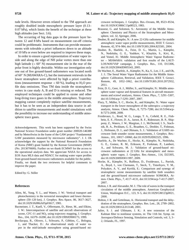
9728 M. Lainer et al.: Trajectory mapping of middle atmospheric H2O
tude levels. However errors related to the TM approach are
roughly doubled inside mesospheric pressure layer (0.13–
0.07 hPa), which limits the benefit of the technique at these
high altitudes (see Sect. 3.6).
The occurring of big data gaps in the pressure layer be-
tween 12 and 8 hPa based on measurement cut-off criteria
could be problematic. Instruments that can provide measure-
ments with tolerable a priori influences down to an altitude
of 10 hPa or even below are required to improve these maps.
In order to ensure a good representation of water vapor in-
side and along the edge of NH polar vortex more than one
high latitude (> 60◦ N) measurement site in the rear of the
polar front is highly desirable. Within our investigation only
one out of five ground-based radiometers was located north
of 60◦ N (MIAWARA-C), but the instrument retrievals in the
lower stratosphere were affected by high a priori contribu-
tions (measurement response < 60 %), leading to H2O pro-
file data omissions. Thus TM data inside the stratospheric
vortex in case study A, B and D is missing or reduced. The
employed techniques could be applied to ozone and other
long-living trace gases in the middle atmosphere. Trajectory
mapping cannot completely replace satellite measurements,
but it has to be seen as an independent data source in ad-
dition to satellite measurements and model simulations with
the possibility to increase our understanding of middle atmo-
spheric trace gases.
Acknowledgements. This work has been supported by the Swiss
National Science Foundation under grant number 200020-146388
and by MeteoSwiss in the frame of the GAW project “Fundamental
GAW parameters measured by microwave radiometry”. J. J. Oh
acknowledges the support by the National Research Foundation
of Korea (NRF) grant funded by the Korean Government (MSIP)
(No. 2013070600). Further on we thank ECMWF for the access to
the operational analysis data. We appreciate NASA for access to
EOS Aura MLS data and NDACC for making water vapor profiles
from ground-based microwave radiometers available for the public.
Finally, we thank the two reviewers for helpful comments to
improve the paper.
Edited by: G. Stiller
References
Allen, M., Yung, Y. L., and Waters, J. W.: Vertical transport and
photochemistry in the terrestrial mesosphere and lower thermo-
sphere (50–120 km), J. Geophys. Res.-Space, 86, 3617–3627,
doi:10.1029/JA086iA05p03617, 1981.
Bacmeister, J. T., Kuell, V., Offermann, D., Riese, M., and Elkins,
J. W.: Intercomparison of satellite and aircraft observations of
ozone, CFC-11 and NOy using trajectory mapping, J. Geophys.
Res., 104, 16379–16390, doi:10.1029/1999JD900173, 1999.
Bevilacqua, R., Olivero, J., Schwartz, P., Gibbins, C., Bologna,
J., and Thacker, D.: An observational study of water va-
por in the mid-latitude mesosphere using ground-based mi-
crowave techniques, J. Geophys. Res.-Oceans, 88, 8523–8534,
doi:10.1029/JC088iC13p08523, 1983.
Brasseur, G. and Solomon, S.: Aeronomy of the Middle Atmo-
sphere: Chemistry and Physics of the Stratosphere and Meso-
sphere, vol. 32, Springer, 2006.
Deuber, B. and Kämpfer, N.: A new 22-GHz radiometer for middle
atmospheric water vapor profile measurements, IEEE T. Geosci.
Remote, 42, 974–984, doi:10.1109/TGRS.2004.825581, 2004.
Deuber, B., Haefele, A., Feist, D. G., Martin, L., Kämpfer,
N., Nedoluha, G. E., Yushkov, V., Khaykin, S., Kivi, R.,
and Vomel, H.: Middle Atmospheric Water Vapour Radiome-
ter – MIAWARA: validation and first results of the LAUT-
LOS/WAVVAP campaign, J. Geophys. Res., 110, D13306,
doi:10.1029/2004JD005543, 2005.
De Wachter, E., Haefele, A., Kämpfer, N., Ka, S., Lee, J. E., and Oh,
J. J.: The Seoul Water Vapor Radiometer for the Middle Atmo-
sphere: Calibration, Retrieval, and Validation, IEEE T. Geosci.
Remote, 49, 1052–1062, doi:10.1109/TGRS.2010.2072932,
2011.
Feist, D. G., Geer, A. J., Müller, S., and Kämpfer, N.: Middle atmo-
sphere water vapour and dynamical features in aircraft measure-
ments and ecmwf analyses, Atmos. Chem. Phys., 7, 5291–5307,
doi:10.5194/acp-7-5291-2007, 2007.
Flury, T., Müller, S. C., Hocke, K., and Kämpfer, N.: Water vapor
transport in the lower mesosphere of the subtropics: a trajectory
analysis, Atmos. Chem. Phys., 8, 7273–7280, doi:10.5194/acp-
8-7273-2008, 2008.
Froidevaux, L., Read, W. G., Lungu, T. A., Cofield, R. E., Fish-
bein, E. F., Flower, D. A., Jarnot, R. F., Ridenoure, B. P., Ship-
pony, Z., Waters, J. W., Margitan, J. J., McDermid, I. S., Stach-
nik, R. A., Peckham, G. E., Braathen, G., Deshler, T., Fishman,
J., Hofmann, D. J., and Oltmans, S. J.: Validation of UARS mi-
crowave limb sounder ozone measurements, J. Geophys. Res.-
Atmos., 101, 10017–10060, doi:10.1029/95JD02325, 1996.
Haefele, A., De Wachter, E., Hocke, K., Kämpfer, N., Nedoluha,
G. E., Gomez, R. M., Eriksson, P., Forkman, P., Lambert,
A., and Schwartz, M. J.: Validation of ground-based mi-
crowave radiometers at 22 GHz for stratospheric and meso-
spheric water vapor, J. Geophys. Res.-Atmos., 114, D23305,
doi:10.1029/2009JD011997, 2009.
Hocke, K., Kämpfer, N., Ruffieux, D., Froidevaux, L., Parrish,
A., Boyd, I., von Clarmann, T., Steck, T., Timofeyev, Y. M.,
Polyakov, A. V., and Kyrölä, E.: Comparison and synergy of
stratospheric ozone measurements by satellite limb sounders
and the ground-based microwave radiometer SOMORA, At-
mos. Chem. Phys., 7, 4117–4131, doi:10.5194/acp-7-4117-2007,
2007.
Holton, J. R. and Alexander, M. J.: The role of waves in the transport
circulation of the middle atmosphere, American Geophysical
Union, Washington D.C., 123, 9–5, doi:10.1029/GM123p0021,
2000.
Holton, J. R. and Gettelman, A.: Horizontal transport and the dehy-
dration of the stratosphere, Geophys. Res. Lett., 28, 2799–2802,
doi:10.1029/2001GL013148, 2001.
Julier, S. J. and Uhlmann, J. K.: A new extension of the
Kalman filter to nonlinear systems, in: The 11th Int. Symp. on
Aerospace/Defence Sensing, Simulation and Controls, vol. 3, 3–
2, Orlando, FL, 1997.
Atmos. Chem. Phys., 15, 9711–9730, 2015 www.atmos-chem-phys.net/15/9711/2015/

M. Lainer et al.: Trajectory mapping of middle atmospheric H2O 9729
Kämpfer, N., Nedoluha, G., Haefele, A., and De Wachter, E.: Mi-
crowave Radiometry, vol. 10 of ISSI Scientific Report Series,
Springer, New York, doi:10.1007/978-1-4614-3909-7, 2012.
Lambert, A., Read, W. G., Livesey, N. J., Santee, M. L., Manney,
G. L., Froidevaux, L., Wu, D. L., Schwartz, M. J., Pumphrey, H.
C., Jimenez, C., Nedoluha, G. E., Cofield, R. E., Cuddy, D. T.,
Daffer, W. H., Drouin, B. J., Fuller, R. A., Jarnot, R. F., Knosp,
B. W., Pickett, H. M., Perun, V. S., Snyder, W. V., Stek, P. C.,
Thurstans, R. P., Wagner, P. A., Waters, J. W., Jucks, K. W., Toon,
G. C., Stachnik, R. A., Bernath, P. F., Boone, C. D., Walker, K.
A., Urban, J., Murtagh, D., Elkins, J. W., and Atlas, E.: Validation
of the Aura Microwave Limb Sounder middle atmosphere water
vapor and nitrous oxide measurements, J. Geophys. Res.-Atmos.,
112, D24S36, doi:10.1029/2007JD008724, 2007.
Liu, G., Tarasick, D. W., Fioletov, V. E., Sioris, C. E., and Ro-
chon, Y. J.: Ozone correlation lengths and measurement uncer-
tainties from analysis of historical ozonesonde data in North
America and Europe, J. Geophys. Res.-Atmos., 114, D04112,
doi:10.1029/2008JD010576, 2009.
Liu, H.-L., Roble, R. G., Taylor, M. J., and Pendleton,
W. R.: Mesospheric planetary waves at Northern Hemi-
sphere fall equinox, Geophys. Res. Lett., 28, 1903–1906,
doi:10.1029/2000GL012689, 2001.
Liu, J., Tarasick, D. W., Fioletov, V. E., McLinden, C., Zhao, T.,
Gong, S., Sioris, C., Jin, J. J., Liu, G., and Moeini, O.: A global
ozone climatology from ozone soundings via trajectory mapping:
a stratospheric perspective, Atmos. Chem. Phys., 13, 11441–
11464, doi:10.5194/acp-13-11441-2013, 2013.
Livesey, N. J., Read, W. G., Froidevaux, L., Lambert, A., Manney,
G. L., Pumphrey, H. C., Santee, M. L., Schwartz, M. J., Wang,
S., Coeld, R. I., Cuddy, D. T., Fuller, R. A., Jarnot, R. F., Jiang,
J. H., Knosp, B. W., Stek, P. C., Wagner, P. A., and Wu, D. L.:
Version 3.3 and 3.4 Level 2 data quality and description docu-
ment, Tech. rep., Jet Propulsion Laboratory, California Institute
of Technology, 2011.
Monge-Sanz, B. M., Chipperfield, M. P., Simmons, A. J., and Up-
pala, S. M.: Mean age of air and transport in a CTM: comparison
of different ECMWF analyses, Geophys. Res. Lett., 34, L04801,
doi:10.1029/2006GL028515, 2007.
Morris, G. A.: A demonstration and evaluation of trajectory map-
ping, PhD thesis, Rice University, 1994.
Morris, G. A., Schoeberl, M. R., Sparling, L. C., Newman, P. A.,
Lait, L. R., Elson, L., Walters, J., Suttie, R. A., Roche, A., Kumer,
J., and Russel, J. M.: Trajectory mapping and applications to data
from the Upper Atmosphere Research Satellite, J. Geophys. Res.,
100, 16491–16505, doi:10.1029/95JD01072, 1995.
Morris, G. A., Gleason, J. F., Ziemke, J., and Schoeberl,
M. R.: Trajectory mapping: A tool for validation of trace
gas observations, J. Geophys. Res., 105, 17875–17894,
doi:10.1029/1999JD901118, 2000.
Mote, P. W., Rosenlof, K. H., McIntyre, M. E., Carr, E. S.,
Gille, J. C., Holton, J. R., Kinnersley, J. S., Pumphrey, H.
C., Russell, J. M., and Waters, J. W.: An atmospheric tape
recorder: the imprint of tropical tropopause temperatures on
stratospheric water vapor, J. Geophys. Res.-Atmos., 101, 3989–
4006, doi:10.1029/95JD03422, 1996.
Nedoluha, G. E., Gomez, R. M., Hicks, B. C., Bevilacqua, R. M.,
Russell, J. M., Connor, B. J., and Lambert, A.: A comparison of
middle atmospheric water vapor as measured by WVMS, EOS-
MLS, and HALOE, J. Geophys. Res.-Atmos., 112, D24S39,
doi:10.1029/2007JD008757, 2007.
Nedoluha, G. E., Gomez, R. M., Hicks, B. C., Wrotny, J. E., Boone,
C., and Lambert, A.: Water vapor measurements in the meso-
sphere from Mauna Loa over solar cycle 23, J. Geophys. Res.-
Atmos., 114, D23303, doi:10.1029/2009JD012504, 2009.
Nedoluha, G. E., Gomez, R. M., Hicks, B. C., Helmboldt,
J., Bevilacqua, R. M., and Lambert, A.: Ground-based mi-
crowave measurements of water vapor from the midstratosphere
to the mesosphere, J. Geophys. Res.-Atmos., 116, D02309,
doi:10.1029/2010JD014728, 2011.
Nedoluha, G. E., Gomez, R. M., Neal, H., Lambert, A., Hurst,
D., Boone, C., and Stiller, G.: Validation of long-term measure-
ments of water vapor from the midstratosphere to the meso-
sphere at two Network for the Detection of Atmospheric Com-
position Change sites, J. Geophys. Res.-Atmos., 118, 934–942,
doi:10.1029/2012JD018900, 2013.
Palm, M., v. Savigny, C., Warneke, T., Velazco, V., Notholt,
J., Künzi, K., Burrows, J., and Schrems, O.: Intercomparison
of O3 profiles observed by SCIAMACHY and ground based
microwave instruments, Atmos. Chem. Phys., 5, 2091–2098,
doi:10.5194/acp-5-2091-2005, 2005.
Paparella, F., Babiano, A., Basdevant, C., Provenzale, A.,
and Tanga, P.: A Lagrangian study of the Antarctic po-
lar vortex, J. Geophys. Res.-Atmos., 102, 6765–6773,
doi:10.1029/96JD03377, 1997.
Petterssen, S.: Weather analysis and forecasting, McGraw-Hill
Book Company, New York, 221–223, 1940.
Rabier, F., Järvinen, H., Klinker, E., Mahfouf, J.-F., and Sim-
mons, A.: The ecmwf operational implementation of four-
dimensional variational assimilation. I: Experimental results with
simplified physics, Q. J. Roy. Meteor. Soc., 126, 1143–1170,
doi:10.1002/qj.49712656417, 2000.
Reinsel, G., Box, G., and Jenkins, G.: Time Series Analysis:
Forecasting and Control, Third Edn., Prentice-Hall, Englewood
Cliffs, 1994.
Revercomb, H. E., Buijs, H., Howell, H. B., LaPorte, D. D., Smith,
W. L., and Sromovsky, L. A.: Radiometric calibration of IR
Fourier transform spectrometers: solution to a problem with
the High-Resolution Interferometer Sounder, Appl. Optics, 27,
3210–3218, doi:10.1364/AO.27.003210, 1988.
Rodgers, C. D.: Inverse Methods for Atmospheric Sounding: The-
ory and Practice, vol. 2, World Scientific, Singapore, 2000.
Rüfenacht, R., Murk, A., Kämpfer, N., Eriksson, P., and Buehler,
S. A.: Middle-atmospheric zonal and meridional wind profiles
from polar, tropical and midlatitudes with the ground-based mi-
crowave Doppler wind radiometer WIRA, Atmos. Meas. Tech.,
7, 4491–4505, doi:10.5194/amt-7-4491-2014, 2014.
Scheiben, D., Straub, C., Hocke, K., Forkman, P., and Kämpfer,
N.: Observations of middle atmospheric H2O and O3 during
the 2010 major sudden stratospheric warming by a network of
microwave radiometers, Atmos. Chem. Phys., 12, 7753–7765,
doi:10.5194/acp-12-7753-2012, 2012.
Schoeberl, M. R.: Stratospheric warmings: observations and theory,
Rev. Geophys., 16, 521–538, doi:10.1029/RG016i004p00521,
1978.
Schoeberl, M. R. and Sparling, L. C.: Trajectory modelling, in: Di-
agnostic Tools in Atmospheric Physics, edited by: Fiocco, G. and
Visconti, G., vol. 1, IOS Press, p. 289, 1995.
www.atmos-chem-phys.net/15/9711/2015/ Atmos. Chem. Phys., 15, 9711–9730, 2015

9730 M. Lainer et al.: Trajectory mapping of middle atmospheric H2O
Stohl, A. and Seibert, P.: Accuracy of trajectories as determined
from the conservation of meteorological tracers, Q. J. Roy. Me-
teor. Soc., 124, 1465–1484, doi:10.1002/qj.49712454907, 1998.
Stohl, A., Wotawa, G., Seibert, P., and Kromp-Kolb, H.: Interpola-
tion errors in wind fields as a function of spatial and temporal
resolution and their impact on different types of kinematic tra-
jectories, J. Appl. Meteorol., 34, 2149–2165, doi:10.1175/1520-
0450(1995)034<2149:IEIWFA>2.0.CO;2, 1995.
Straub, C., Murk, A., and Kämpfer, N.: MIAWARA-C, a new
ground based water vapor radiometer for measurement cam-
paigns, Atmos. Meas. Tech., 3, 1271–1285, doi:10.5194/amt-3-
1271-2010, 2010.
Sutton, R. T., Maclean, H., Swinbank, R., O’Neill, A., and Tay-
lor, F. W.: High-resolution stratospheric tracer fields estimated
from satellite observations using Lagrangian trajectory cal-
culations, J. Atmos. Sci., 51, 2995–3005, doi:10.1175/1520-
0469(1994)051<2995:HRSTFE>2.0.CO;2, 1994.
Tschanz, B., Straub, C., Scheiben, D., Walker, K. A., Stiller, G. P.,
and Kämpfer, N.: Validation of middle-atmospheric campaign-
based water vapour measured by the ground-based microwave
radiometer MIAWARA-C, Atmos. Meas. Tech., 6, 1725–1745,
doi:10.5194/amt-6-1725-2013, 2013.
Wang, P. K.: Moisture plumes above thunderstorm anvils and
their contributions to cross-tropopause transport of water va-
por in midlatitudes, J. Geophys. Res.-Atmos., 108, 4194,
doi:10.1029/2002JD002581, 2003.
Wernli, H. and Davies, H. C.: A Lagrangian-based analysis of ex-
tratropical cyclones. I: The method and some applications, Q. J.
Roy. Meteor. Soc., 123, 467–489, doi:10.1002/qj.49712353811,
1997.
Atmos. Chem. Phys., 15, 9711–9730, 2015 www.atmos-chem-phys.net/15/9711/2015/