Long-term trends in the atmospheric water vapor

content estimated from ground-based GPS data

T. Nilsson1 and G. Elgered1

Received 12 March 2008; revised 29 June 2008; accepted 16 July 2008; published 1 October 2008.

[1] We have used 10 years of ground-based data from the Global Positioning System(GPS) to estimate time series of the excess propagation path due to the gases in the neutralatmosphere. We first derive the excess path caused by water vapor which in turn is used toinfer the water vapor content above each one of 33 GPS receiver sites in Finland andSweden. Although a 10 year period is much too short to search for climate change we usethe data set to assess the stability and consistency of the linear trend of the watervapor content that can be estimated from the data. The linear trends in the integrated watervapor content range from �0.2 to +1.0 kg m�2 decade�1. As one may expect we finddifferent systematic patterns for summer and winter data. The formal uncertainty of thesetrends, taking the temporal correlation of the variability about the estimated model intoaccount, are of the order of 0.4 kg m�2 decade�1. Mostly, this uncertainty is due to thenatural short-term variability in the water vapor content, while the formal uncertainties inthe GPS measurements have only a small impact on the trend errors.

Citation: Nilsson, T., and G. Elgered (2008), Long-term trends in the atmospheric water vapor content estimated from ground-based

GPS data, J. Geophys. Res., 113, D19101, doi:10.1029/2008JD010110.

1. Introduction

[2] Water vapor in the atmosphere is a parameter of greatimportance in climate models because of its role as agreenhouse gas. In fact water vapor is a very efficientgreenhouse gas. An increase of 20% of the water vaporcontent in the tropics has a larger impact than a doubling ofthe carbon dioxide concentration [Buehler et al., 2006]. Inthis presentation we will focus on the integrated water vapor(IWV).[3] The direct human influence on the IWV is almost

negligible [Intergovernmental Panel on Climate Change,2007]. However, water vapor feedback is one of the mostimportant climate feedback processes. An increase of tem-perature due to, e.g., emission of other greenhouse gaseswill result in an increase in IWV since the equilibrium vaporpressure increases with increasing temperature. Typicallyclimate models tend to predict that the average relativehumidity is conserved when the temperature changes[Trenberth et al., 2003]. The relationship between changesin the IWV and changes in the temperature was recentlyassessed byMears et al. [2007]. They found that an increaseof the temperature of 1 K will result in an IWV increase by5–7%. Using long time series of IWV and temperature thisdependence can be tested. Furthermore, if the relativehumidity is conserved, long time series of IWV measure-ments can be used as an independent data source to detectglobal warming. In all applications for monitoring of

climate change high long-term stability of the measurementsis needed.[4] A number of different studies to measure trends in

IWV have been performed. Ross and Elliott [1996] studiedthe trends in IWV over North America as measured byradiosondes. Their analysis was later extended to the wholeNorthern Hemisphere [Ross and Elliott, 2001]. Overall theyfound an increase of IWV for the period 1973–1995,although there were large regional variations and evennegative trends in some regions. However, extending thisanalysis to include periods after 1995 is problematic becauseof large changes in the radiosonde types at the end of 1995and later [Elliott et al., 2002; Trenberth et al., 2005].Bengtsson et al. [2004] studied temperature and IWV trendsobtained from the ERA40 data set and found a globalincrease in IWV (+0.36 kg m�2 decade�1) which was twiceas large as could be expected from the global temperaturetrend (+0.11 K decade�1). The likely reason for this wasidentified as an artifact caused by the changes in the globalobserving systems over the last decades. Similar conclu-sions were drawn by Trenberth et al. [2005] who comparedtrends obtained from ERA40, NCEP reanalysis, satellitemeasurements and the radiosonde data used by Ross andElliott [2001].[5] Global Navigation Satellite Systems (GNSS) can be

used as a tool to estimate the IWV in the atmosphere. Mostof the observations and studies on the accuracy of GNSSestimation of IWV carried out so far have used data fromthe Global Positioning System (GPS) [see, e.g., Tralli andLichten, 1990; Bevis et al., 1992; Emardson et al., 1998;Hagemann et al., 2003; Gutman et al., 2004]. Today thereare many national and international GPS networks that havebeen operating for more than 10 years.

JOURNAL OF GEOPHYSICAL RESEARCH, VOL. 113, D19101, doi:10.1029/2008JD010110, 2008ClickHere

for

FullArticle

1Onsala Space Observatory, Department of Radio and Space Science,Chalmers University of Technology, Onsala, Sweden.

Copyright 2008 by the American Geophysical Union.0148-0227/08/2008JD010110$09.00

D19101 1 of 12

[6] Relatively few investigations of trends estimatedusing GPS have been performed to date. Gradinarsky etal. [2002] investigated IWV trends over Sweden for theyears 1993–2001, and found positive trends in general. Jinet al. [2007] used estimated trends in the Zenith Total Delay(ZTD) from a large number of globally distributed GPSsites, and found an average ZTD trend of 15 mm decade�1

(corresponding to an IWV trend of 2 kg m�2 decade�1,assuming that the average hydrostatic delay does notchange). There were, however, large regional variationsincluding large negative trends at some sites. A compar-ison of trends estimated by GPS and the similar techniqueVLBI (Very Long Baseline Interferometry) was done bySteigenberger et al. [2007]. They showed that the trendsestimated using the two techniques only agree when ZTDestimates from both techniques are available simultaneously,demonstrating that the estimated trend is very sensitive tothe time period used. The same conclusions were drawn byHaas et al. [2003].[7] In this work we study the trends in IWV estimated

using GPS data from Sweden and Finland acquired over a10 year period. We begin in section 2 with a summary of thebackground theory. In section 3 we describe the analysis ofGPS data. Thereafter, in section 4, the derivation of IWVfrom the estimated propagation delays is described togetherwith examples of IWV time series. Sections 5 and 6 presentthe estimation of linear trends and their uncertainties,

respectively. The results are discussed in section 7, andsection 8 ends the paper with the conclusions.

2. Theoretical Background

[8] The atmospheric parameter estimated in the GPS dataprocessing is the equivalent excess propagation path referredto the zenith direction, often called the Zenith Total Delay(ZTD). It is often expressed in units of length, using thespeed of light in vacuum for the conversion from a timedelay. The ZTD, ‘t, can be divided into a Zenith HydrostaticDelay (ZHD), ‘h, and a Zenith Wet Delay (ZWD), ‘w [Daviset al., 1985]:

‘t ¼ ‘h þ ‘w ð1Þ

[9] The hydrostatic term can be determined with anuncertainty of less than 1 mm in the zenith direction if thetotal ground pressure is measured with an uncertainty of lessthan 0.5 hPa [Davis et al., 1985]. The ZWD can be writtenas [Elgered, 1993]:

‘w ¼ 24 � 10�6

Z1

0

e

Tdhþ 0:3754

Z1

0

e

T2dh m½ ð2Þ

where e is of the partial pressure of water vapor and T is thetemperature, expressed in hPa and K, respectively. Theexpression for the IWV is similar:

V ¼Z1

0

rvdh ð3Þ

where rv is the absolute humidity in kg m�3. The ZWD isrelated to the IWV because, according to the ideal gas law,rv is proportional to e/T. A conversion factor Q:

Q ¼ ‘wV

ð4Þ

can be calculated by assuming a value of the meantemperature of the wet refractivity in the atmosphere. Thisconversion factor can be modeled, e.g., using a history ofradiosonde data [Emardson and Derks, 2000], or calculatedusing reanalysis data from a numerical weather model suchas the ECMWF model [Wang et al., 2005]. These studieshave shown that the IWV can be estimated from the ZWDwith a typical root-mean-square (RMS) conversion error ofless than 2%.

3. Analysis of GPS Data From SWEPOS andFinnRef

[10] We have used data from 33 GPS receiver sites inSweden and Finland. The sites are of geodetic quality,meaning that they are mounted on solid bedrock. Most ofthe Swedish and Finnish sites have been in continuousoperation since late 1993 and late 1996, respectively.Figure 1 shows the sites. Their names and coordinates are

Figure 1. GPS receiver sites in the Swedish SWEPOSnetwork and the Finnish FinnRef network.

D19101 NILSSON AND ELGERED: TRENDS IN WATER VAPOR FROM GPS DATA

2 of 12

D19101

listed in Table 1. For more details about the networks [see,e.g., Johansson et al., 2002].[11] The GPS data were analyzed using the GAMIT GPS

processing software, developed at the Massachusetts Insti-tute of Technology [Herring et al., 2006]. The software isbased on a method referred to as a network solution. Thismeans that many sites are processed together. Since theprocessing time increases rapidly as the number of sites inthe network increases, it is convenient to divide the networkinto subnetworks and process each one separately [Lidberg,2007]. In our case all SWEPOS sites are processed in onesolution and all FinnRef sites in another. Six of theSWEPOS sites have also been included in the FinnRefsolution in order to be able to compare the two solutions.All observations are included down to an elevation cutoffangle of 10� and the elevation dependencies of the ZHD andthe ZWD were modeled using the mapping functionsdeveloped by Niell [1996]. In the analysis site coordinates,satellite coordinates, integer ambiguities, and the ZTD areestimated. An elevation-dependent weighting of the GPSobservations was used. The weights were determined foreach site and each day from a preliminary solution. Fordetails about the data processing, see Lidberg et al. [2007]and Lidberg [2007].[12] We chose to use the data from the 10 year period 17

November 1996 to 16 November 2006. The data acquiredwith SWEPOS from the first 3 years (before 17 November1996) were not used in order to cover the same time periodwith all sites. Furthermore, there were a number of antenna

radome changes during 1993–1996 which have a signifi-cant impact on the estimated values of the IWV whenperforming network solutions [Emardson et al., 2000].

4. Deriving the Water Vapor Content FromZenith Total Delays

[13] In order to obtain the ZWD from the estimated ZTDwe use the total pressure at the GPS antenna to calculate andsubtract the ZHD. A pressure error of 1 hPa results in anerror of 2.3 mm in the ZHD, and hence also in the ZWD,which is equivalent to an IWV error of 0.35 kg m�2.[14] The majority of the SWEPOS and FinnRef sites are

not equipped with barometers, hence direct pressure meas-urements are not available. One possible way to obtainpressure data is to use the results from numerical weathermodels. In this work we have used pressure estimates

Table 1. GPS Sites, Sorted by Decreasing Latitude

Site

Longitude (�E) Latitude (�N) Heighta (m)Acronym Full Name

KEVO Kevo 27.007 69.756 111KIR0 Kiruna 21.060 67.877 469SODA Sodankyla 26.389 67.421 279ARJ0 Arjeplog 18.125 66.318 459OVE0 Over Kalix 22.770 66.310 200KUUS Kuusamo 29.033 65.910 361OULU Oulu 25.893 65.086 71SKE0 Skelleftea 21.050 64.880 59VIL0 Vilhelmina 16.559 64.697 420ROMU Romuvaara 29.932 64.217 224UME0 Umea 19.509 63.578 32OST0 Ostersund 14.858 63.442 459VAAS Vaasa 21.771 62.961 40KIVE Kivetty 25.702 62.820 198JOEN Joensuu 30.096 62.391 97SUN0 Sundsvall 17.659 62.232 7SVE0 Sveg 14.700 62.017 458OLKI Olkiluoto 21.473 61.240 12LEK0 Leksand 14.877 60.722 448MAR6 Martsbo 17.258 60.595 51VIRO Virolahti 27.555 60.539 22TUOR Tuorla 22.443 60.416 41METS Metsahovi 24.395 60.217 76KAR0 Karlstad 13.505 59.444 83LOV0 Lovo 17.830 59.340 56VAN0 Vanersborg 12.070 58.690 135NOR0 Norrkoping 16.250 58.590 13JON0 Jonkoping 14.059 57.745 227SPT0 Boras 12.891 57.715 185VIS0 Visby 18.367 57.653 55ONSA Onsala 11.925 57.395 9OSK0 Oskarshamn 16.000 57.060 120HAS0 Hassleholm 13.718 56.092 79aThe heights are referenced to the mean sea level.

Figure 2. Comparison between modeled and measuredpressure at the Onsala site. (a) The differences areoccasionally large because of the 3 h temporal resolutionof the model. (b) The largest difference is caused by rapidvariations during the passage of a low-pressure weathersystem.

D19101 NILSSON AND ELGERED: TRENDS IN WATER VAPOR FROM GPS DATA

3 of 12

D19101

obtained from a model used by the Swedish Meteorologicaland Hydrological Institute (SMHI). However, it is notobvious that the pressure values obtained from this modelare accurate enough. For example, Hagemann et al. [2003]found that pressure estimated from the ECMWF (EuropeanCentre for Medium Range Weather Forecasts) operationalanalysis did contain too large errors (several hPa). Themodel used in this work does however have a betterresolution than the ECMWF model.[15] To test the accuracy of the pressure estimates

obtained from SMHI, we made a comparison to indepen-dent local pressure measurements at the Onsala site(ONSA). The differences between the two time series areshown in Figure 2a. They agree with an RMS difference of0.42 hPa. We note occasional large differences of severalhPa. These are caused by the limited temporal resolution(3 h) of the SMHI model which fails to correctly model therapid pressure variation associated with a passing low-pressure system. This is illustrated in Figure 2b, showingthe period with the largest difference in mid 1998. Theestimated linear trend of the difference is �0.0074 hPa a�1.If this were a long-term drift it would introduce an error of�0.17 mm decade�1 in the ZWD trend and �0.026 kg m�2

decade�1 in the IWV trend, if not corrected for. However,

we chose not to make any such corrections. It is difficult todetermine if it is a true long-term drift in the model or in thebarometer measurements. Furthermore, if we assume thatthe errors are correlated over a few days, the observed driftis comparable to its uncertainty. Given the size of the drift, itis not of large importance for our application because it issignificantly below the uncertainties in the linear trendsestimated from the GPS data, as we will show below. Weconclude that the pressure estimates obtained from SMHIare accurate enough to be used in our study. However,future investigations shall assess the accuracy of the SMHIpressure estimates also at other locations.[16] The next conversion, from ZWD to IWV will also

introduce an error in the trend estimates through anyunmodeled trend in the conversion factor. Since the con-version factor (4) depends on a mean temperature of the wetrefractivity in the atmosphere, it will be affected by apossible trend in the temperature. An unmodeled meantemperature change of 1 K will introduce an error in theconversion factor of about 0.4%. Assuming that the tem-

Figure 3. Lomb-Scargle periodograms for the IWV timeseries from (a) Arjeplog and (b) Hassleholm.

Figure 4. IWV time series from (a) Arjeplog and(b) Hassleholm. The straight line is the fitted linear drift,and the periodic function models the seasonal variability inaccordance with equation (5).

D19101 NILSSON AND ELGERED: TRENDS IN WATER VAPOR FROM GPS DATA

4 of 12

D19101

perature change over the last decade is less than 1 K, theerror in the IWV trends caused by a trend in the conversionfactor will be much smaller than the IWV trends we observe(see below). This whole problem can of course be avoided ifZWD is analyzed rather than the IWV. We have, however,done the conversion to IWV using Emardson et al. [1998,equation (3)]. This equation is slightly less accurate com-pared to those using ground temperatures. However, wechose this path rather than risking introducing any trendsfrom such a local point observation.

5. Estimation of Linear Trends in IWV

[17] In order to obtain the linear trends from the GPS timeseries we need to consider the annual variations in watervapor, especially if there are gaps in the time series (or if thelength of the investigated period would not be an integernumber of years). In order to investigate how many terms ina Fourier expansion that are needed in order to describe theannual variation of the IWV (annual term, semiannual termetc.), and also to investigate if there are any other periodicvariations on time scales 1 year, we calculated the Lomb-Scargle periodograms [Hocke, 1998] from the time series.Two examples are shown in Figure 3. We can clearly see apeak for the annual period, and also one much smaller at thesemiannual period. No other significant peaks are seen,

indicating that it is sufficient to use an annual and asemiannual term to describe the seasonal variations. Wenote that the semiannual term is relatively stronger at theArjeplog site, in the north of Sweden, compared to theresults for the Hassleholm site in the south.[18] We also investigated to use a logarithmic scale in the

analysis, i.e., studying log(V +D) instead of in V because thismay suppress the semiannual term. The constantD should bechosen so that the variability of log(V + D) is relativelyconstant over the year. We found that this approach indeeddecreased the semiannual term, especially when a D closeto zero is used. However, the semiannual term was generallystill significant and needed to be estimated. Furthermore,there were only small differences in the trends estimatedusing a logarithmic scale or a linear scale (at the most thesediffered by 0.1 kg m�2 decade�1). Hence, we have usedIWV in a linear scale when estimating the trends but notethat a logarithmic scale may be investigated further usingother data sets.[19] On the basis of the results from the periodograms,

the following model is used with the ZWD and the IWVtime series:

V ¼ V0 þ a1t þ a2 sin 2ptð Þ þ a3 cos 2ptð Þþ a4 sin 4ptð Þ þ a5 cos 4ptð Þ ð5Þ

Table 2. Model Parameters Describing the Estimated Long-Term Trends and Annual Systematics in the Equivalent ZWD and the IWV

Sitea

Zenith Wet Delay Integrated Water Vapor

RelativeTrend

(% decade�1)

Meanb

‘w,0(mm)

Trenda‘w,1(mm

decade�1)

Annual Semiannual

Meanb V0

(kg m�2)

Trend aV1(kg m�2

decade�1)

Annual Semiannual

a‘w,2(mm)

a‘w,3(mm)

a‘w,4(mm)

a‘w,5(mm)

aV2(kg m�2)

aV3(kg m�2)

aV4(kg m�2)

aV5(kg m�2)

KEVO 65.60 3.83 �22.4 �38.6 9.3 7.5 9.91 0.58 �3.5 �6.0 1.5 1.2 5.8KIR0 64.22 2.42 �19.2 �34.6 8.7 9.2 9.72 0.37 �3.0 �5.4 1.4 1.4 3.8SODA 67.33 2.31 �23.0 �41.0 8.3 8.4 10.21 0.35 �3.6 �6.4 1.3 1.3 3.4ARJ0 65.41 2.54 �19.7 �34.5 8.7 8.0 9.93 0.39 �3.1 �5.4 1.4 1.3 3.9OVE0 72.79 2.43 �22.3 �39.9 9.5 9.2 11.05 0.37 �3.5 �6.3 1.5 1.4 3.3KUUS 64.27 0.72 �21.8 �41.4 7.3 8.0 9.77 0.11 �3.4 �6.5 1.2 1.3 1.1OULU 74.18 2.90 �24.0 �43.3 9.4 8.5 11.29 0.45 �3.7 �6.8 1.5 1.3 3.9SKE0 78.32 2.93 �23.7 �42.1 9.2 10.0 11.92 0.45 �3.7 �6.6 1.5 1.6 3.7VIL0 70.25 3.85 �20.3 �34.8 8.2 8.1 10.69 0.59 �3.2 �5.5 1.3 1.3 5.5ROMU 71.68 0.90 �22.5 �43.1 8.5 8.3 10.92 0.15 �3.5 �6.8 1.4 1.3 1.3UME0 81.43 2.00 �24.5 �41.8 9.5 9.1 12.42 0.31 �3.8 �6.6 1.5 1.4 2.5OST0 71.21 2.77 �20.1 �33.8 8.7 7.4 10.86 0.43 �3.2 �5.4 1.4 1.2 3.9VAAS 79.07 5.94 �25.7 �41.8 9.3 8.3 12.07 0.91 �4.0 �6.6 1.5 1.3 7.5KIVE 73.56 2.76 �23.7 �43.1 8.0 7.6 11.24 0.43 �3.7 �6.8 1.3 1.2 3.8JOEN 76.68 3.09 �24.6 �45.4 9.1 10.4 11.72 0.48 �3.9 �7.1 1.5 1.6 4.0SUN0 83.44 2.51 �25.1 �41.5 9.3 8.4 12.75 0.39 �3.9 �6.6 1.5 1.3 3.0SVE0 72.51 3.33 �20.9 �35.4 8.3 7.7 11.08 0.51 �3.3 �5.6 1.3 1.2 4.6OLKI 81.76 5.21 �25.5 �42.0 8.6 8.2 12.51 0.81 �4.0 �6.7 1.4 1.3 6.4LEK0 74.43 2.93 �21.5 �35.8 7.2 7.7 11.40 0.45 �3.4 �5.7 1.2 1.2 3.9MAR6 84.95 2.56 �24.3 �42.4 8.3 9.2 13.02 0.40 �3.8 �6.7 1.3 1.5 3.0VIRO 84.23 4.51 �24.0 �44.5 8.1 10.3 12.91 0.70 �3.8 �7.1 1.3 1.6 5.4TUOR 79.26 2.57 �24.4 �41.6 8.4 9.2 12.15 0.41 �3.8 �6.6 1.4 1.4 3.2METS 80.16 0.28 �24.0 �42.7 7.9 10.0 12.29 0.06 �3.8 �6.8 1.3 1.6 0.4KAR0 86.70 3.83 �24.5 �40.4 7.4 7.5 13.31 0.59 �3.9 �6.5 1.2 1.2 4.4LOV0 88.43 �1.07 �24.5 �41.1 7.6 9.1 13.57 �0.16 �3.9 �6.6 1.2 1.4 �1.2VAN0 86.68 1.90 �23.5 �38.6 6.6 6.8 13.32 0.30 �3.7 �6.2 1.1 1.1 2.2NOR0 89.82 0.03 �24.9 �42.4 7.6 8.6 13.81 0.01 �4.0 �6.8 1.2 1.4 0.0JON0 85.16 1.27 �22.8 �39.3 6.2 7.4 13.11 0.20 �3.6 �6.3 1.0 1.2 1.5SPT0 89.30 0.82 �23.5 �38.8 6.9 6.8 13.74 0.14 �3.7 �6.2 1.1 1.1 0.9VIS0 88.65 �1.28 �24.7 �40.9 6.7 8.6 13.65 �0.19 �3.9 �6.5 1.1 1.4 �1.4ONSA 88.63 3.71 �24.9 �40.1 6.8 6.7 13.65 0.58 �4.0 �6.4 1.1 1.1 4.2OSK0 89.80 �0.93 �24.3 �41.6 6.5 7.5 13.84 �0.14 �3.9 �6.7 1.1 1.2 �1.0HAS0 91.85 0.41 �24.5 �40.3 6.1 6.0 14.17 0.07 �3.9 �6.5 1.0 1.0 0.4

aThe site names are identified in Table 1 and their locations are seen in the map in Figure 1.bMean values refers to the time epoch t = 0, which in this work is 1 January 1997.

D19101 NILSSON AND ELGERED: TRENDS IN WATER VAPOR FROM GPS DATA

5 of 12

D19101

where t is the time in years and the coefficients V0, a1, a2,a3, a4, and a5, are estimated using the method of leastsquares.[20] Two examples of the original time series and the

fitted models are presented in Figure 4. As seen the fitfollows the seasonal pattern well, however there are alsovariations on time scales of a few weeks or less which are ofcourse not described by the model.[21] We have estimated trends as well as the other model

parameters in both the ZWD and the IWV for the differentsites shown in Figure 1. The results are given in Table 2.The average ZWD/IWV typically is larger for the sites inthe south compared to the sites in the north, as expected.Furthermore, the seasonal variations show more water vaporin the summer compared to the winter, also as expected. Thesemiannual terms are little bit larger at the northern sitesbecause the period of higher IWV in summer is shorter atthe northern sites than at the southern ones (see Figure 4).The ratio between the amplitudes of the annual and semi-annual terms agree with what is expected from the Lomb-Scargle periodograms.[22] When studying the values of the estimated trends we

note that the relative values of the ZWD trends and the IWV

trends are almost identical. This is expected because theconversion algorithm used to derive the IWV from theZWD does only include the site latitude and the time ofthe year. Hence, in Table 2 we give only one relative trend,valid for both the ZWD and the IWV. In the following wefocus on the estimated trends in the IWV.[23] The trends in the IWV for the full 10 year time

period fall in the range from �0.2 to +1.0 kg m�2 decade�1.Figure 5 shows the geographical pattern of these trends. Thetrends at sites located close to each other are similar andthere are differences in the trends at sites in the northern partof the area compared to sites in the southern part. The trendsare largest for the northwestern sites and around the siteVaasa, while the trends at the sites in the southeast ofSweden are slightly negative.[24] The sensitivity of the trends to the selected time

period is demonstrated in Figure 6 and in Table 3, where thetrends obtained using only the first 8 years or the last 8 yearsof the period are shown. The trends obtained using datafrom only the last 8 years are much smaller than thoseobtained using the first 8 years, or the whole 10 year period.The reason is that a 10 (or 8) year period is too short. A verywet or dry year in the beginning or the end of the period will

Figure 5. Estimated IWV trends (in kg m�2 decade�1) in Sweden and Finland for the period17 November 1996 to 16 November 2006.

D19101 NILSSON AND ELGERED: TRENDS IN WATER VAPOR FROM GPS DATA

6 of 12

D19101

Figure 6. Estimated IWV trends (in kg m�2 decade�1) using subsets of the available 10 years of data:(a) 17 November 1996 to 16 November 2004 and (b) 17 November 1998 to 16 November 2006.

D19101 NILSSON AND ELGERED: TRENDS IN WATER VAPOR FROM GPS DATA

7 of 12

D19101

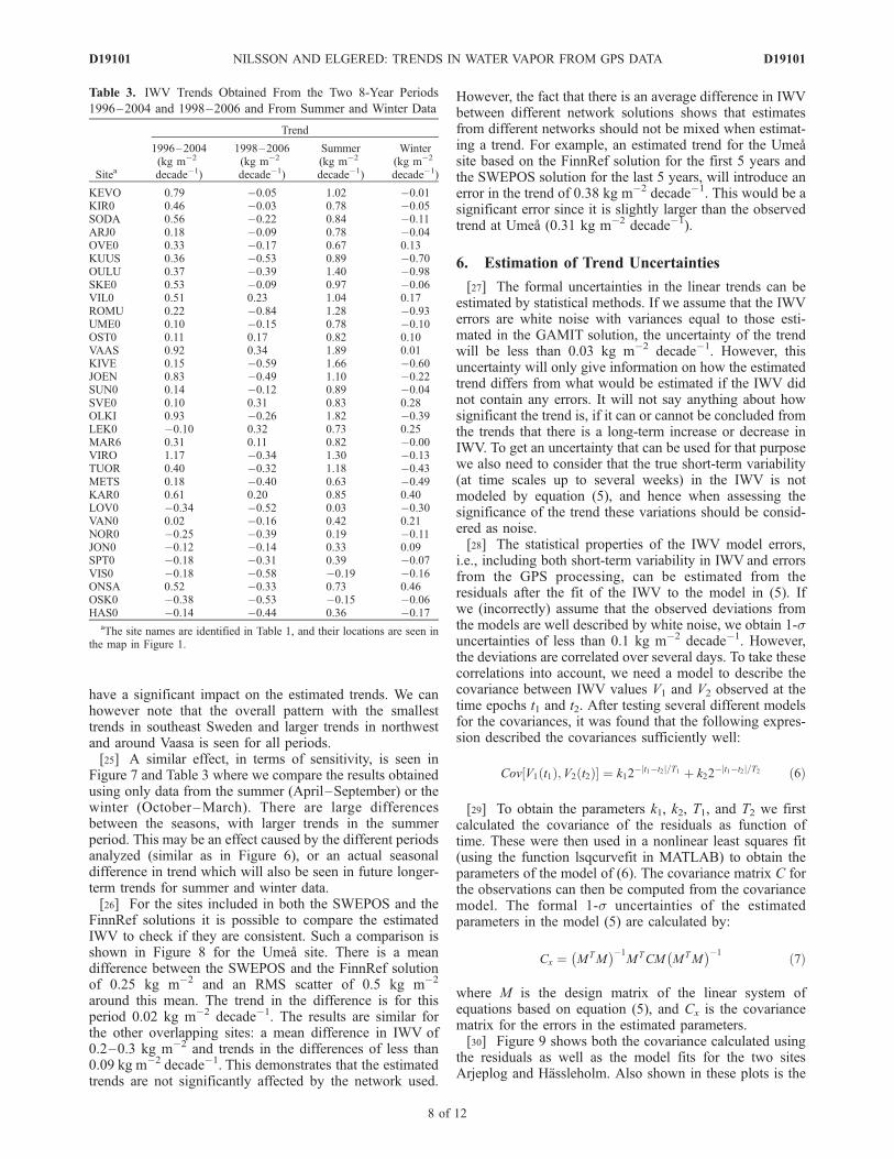
have a significant impact on the estimated trends. We canhowever note that the overall pattern with the smallesttrends in southeast Sweden and larger trends in northwestand around Vaasa is seen for all periods.[25] A similar effect, in terms of sensitivity, is seen in

Figure 7 and Table 3 where we compare the results obtainedusing only data from the summer (April–September) or thewinter (October–March). There are large differencesbetween the seasons, with larger trends in the summerperiod. This may be an effect caused by the different periodsanalyzed (similar as in Figure 6), or an actual seasonaldifference in trend which will also be seen in future longer-term trends for summer and winter data.[26] For the sites included in both the SWEPOS and the

FinnRef solutions it is possible to compare the estimatedIWV to check if they are consistent. Such a comparison isshown in Figure 8 for the Umea site. There is a meandifference between the SWEPOS and the FinnRef solutionof 0.25 kg m�2 and an RMS scatter of 0.5 kg m�2

around this mean. The trend in the difference is for thisperiod 0.02 kg m�2 decade�1. The results are similar forthe other overlapping sites: a mean difference in IWV of0.2–0.3 kg m�2 and trends in the differences of less than0.09 kg m�2 decade�1. This demonstrates that the estimatedtrends are not significantly affected by the network used.

However, the fact that there is an average difference in IWVbetween different network solutions shows that estimatesfrom different networks should not be mixed when estimat-ing a trend. For example, an estimated trend for the Umeasite based on the FinnRef solution for the first 5 years andthe SWEPOS solution for the last 5 years, will introduce anerror in the trend of 0.38 kg m�2 decade�1. This would be asignificant error since it is slightly larger than the observedtrend at Umea (0.31 kg m�2 decade�1).

6. Estimation of Trend Uncertainties

[27] The formal uncertainties in the linear trends can beestimated by statistical methods. If we assume that the IWVerrors are white noise with variances equal to those esti-mated in the GAMIT solution, the uncertainty of the trendwill be less than 0.03 kg m�2 decade�1. However, thisuncertainty will only give information on how the estimatedtrend differs from what would be estimated if the IWV didnot contain any errors. It will not say anything about howsignificant the trend is, if it can or cannot be concluded fromthe trends that there is a long-term increase or decrease inIWV. To get an uncertainty that can be used for that purposewe also need to consider that the true short-term variability(at time scales up to several weeks) in the IWV is notmodeled by equation (5), and hence when assessing thesignificance of the trend these variations should be consid-ered as noise.[28] The statistical properties of the IWV model errors,

i.e., including both short-term variability in IWV and errorsfrom the GPS processing, can be estimated from theresiduals after the fit of the IWV to the model in (5). Ifwe (incorrectly) assume that the observed deviations fromthe models are well described by white noise, we obtain 1-suncertainties of less than 0.1 kg m�2 decade�1. However,the deviations are correlated over several days. To take thesecorrelations into account, we need a model to describe thecovariance between IWV values V1 and V2 observed at thetime epochs t1 and t2. After testing several different modelsfor the covariances, it was found that the following expres-sion described the covariances sufficiently well:

Cov V1 t1ð Þ;V2 t2ð Þ½ ¼ k12�jt1�t2 j=T1 þ k22

�jt1�t2 j=T2 ð6Þ

[29] To obtain the parameters k1, k2, T1, and T2 we firstcalculated the covariance of the residuals as function oftime. These were then used in a nonlinear least squares fit(using the function lsqcurvefit in MATLAB) to obtain theparameters of the model of (6). The covariance matrix C forthe observations can then be computed from the covariancemodel. The formal 1-s uncertainties of the estimatedparameters in the model (5) are calculated by:

Cx ¼ MTM� ��1

MTCM MTM� ��1 ð7Þ

where M is the design matrix of the linear system ofequations based on equation (5), and Cx is the covariancematrix for the errors in the estimated parameters.[30] Figure 9 shows both the covariance calculated using

the residuals as well as the model fits for the two sitesArjeplog and Hassleholm. Also shown in these plots is the

Table 3. IWV Trends Obtained From the Two 8-Year Periods

1996–2004 and 1998–2006 and From Summer and Winter Data

Sitea

Trend

1996–2004(kg m�2

decade�1)

1998–2006(kg m�2

decade�1)

Summer(kg m�2

decade�1)

Winter(kg m�2

decade�1)

KEVO 0.79 �0.05 1.02 �0.01KIR0 0.46 �0.03 0.78 �0.05SODA 0.56 �0.22 0.84 �0.11ARJ0 0.18 �0.09 0.78 �0.04OVE0 0.33 �0.17 0.67 0.13KUUS 0.36 �0.53 0.89 �0.70OULU 0.37 �0.39 1.40 �0.98SKE0 0.53 �0.09 0.97 �0.06VIL0 0.51 0.23 1.04 0.17ROMU 0.22 �0.84 1.28 �0.93UME0 0.10 �0.15 0.78 �0.10OST0 0.11 0.17 0.82 0.10VAAS 0.92 0.34 1.89 0.01KIVE 0.15 �0.59 1.66 �0.60JOEN 0.83 �0.49 1.10 �0.22SUN0 0.14 �0.12 0.89 �0.04SVE0 0.10 0.31 0.83 0.28OLKI 0.93 �0.26 1.82 �0.39LEK0 �0.10 0.32 0.73 0.25MAR6 0.31 0.11 0.82 �0.00VIRO 1.17 �0.34 1.30 �0.13TUOR 0.40 �0.32 1.18 �0.43METS 0.18 �0.40 0.63 �0.49KAR0 0.61 0.20 0.85 0.40LOV0 �0.34 �0.52 0.03 �0.30VAN0 0.02 �0.16 0.42 0.21NOR0 �0.25 �0.39 0.19 �0.11JON0 �0.12 �0.14 0.33 0.09SPT0 �0.18 �0.31 0.39 �0.07VIS0 �0.18 �0.58 �0.19 �0.16ONSA 0.52 �0.33 0.73 0.46OSK0 �0.38 �0.53 �0.15 �0.06HAS0 �0.14 �0.44 0.36 �0.17

aThe site names are identified in Table 1, and their locations are seen inthe map in Figure 1.

D19101 NILSSON AND ELGERED: TRENDS IN WATER VAPOR FROM GPS DATA

8 of 12

D19101

Figure 7. Estimated IWV trends (in kg m�2 decade�1) using seasonal data: (a) summer data and(b) winter data.

D19101 NILSSON AND ELGERED: TRENDS IN WATER VAPOR FROM GPS DATA

9 of 12

D19101

model result obtained if only one term is used in thecovariance model. When taking these covariances intoaccount, using the two term model described by (6), theformal 1-s error is approximately 0.4–0.5 kg m�2 decade�1

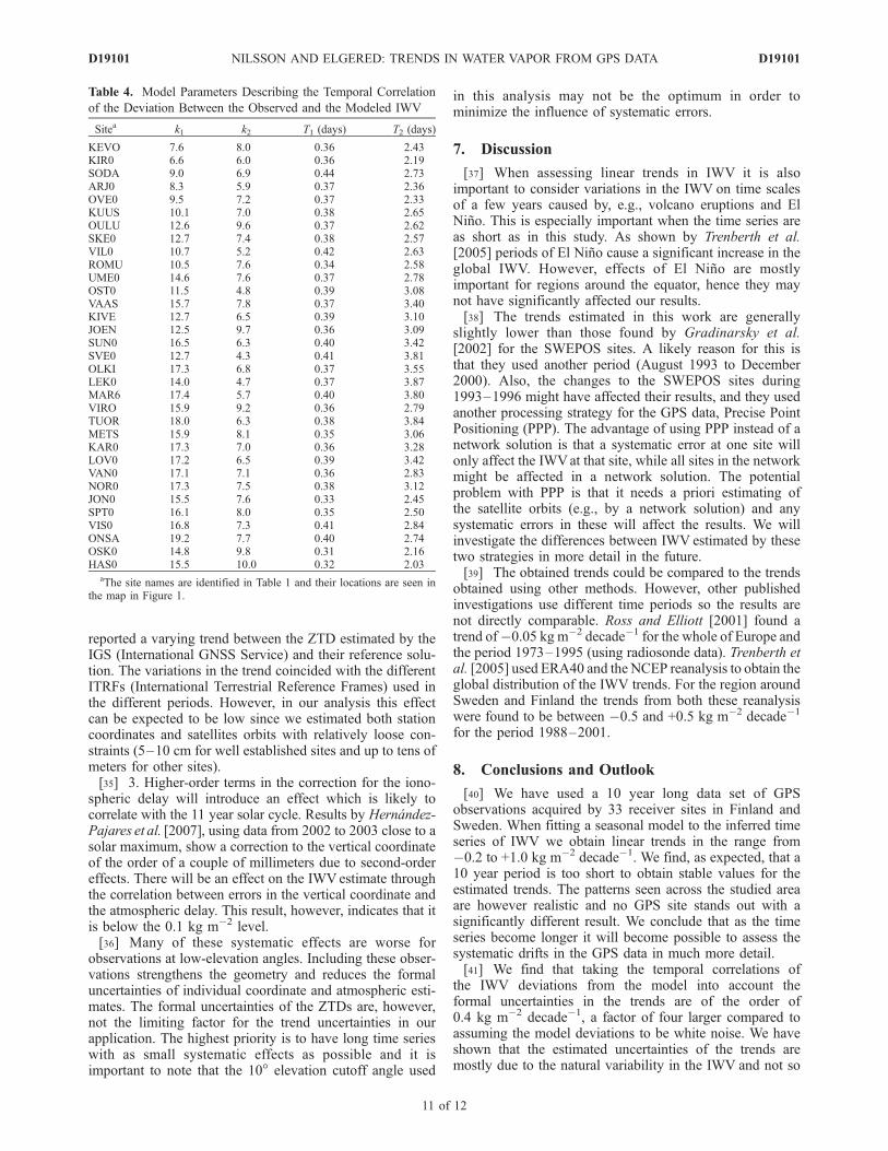
for the 10 year long data set, i.e., at least a factor of fourlarger than when assuming the deviations to be white noise.A similar study, using 8 years of GPS data from SouthAfrica, resulted in an increase by a factor of two describingthe deviations with an ARMA(1, 1) model [Combrink et al.,2007]. The weather conditions in South Africa are howeversignificantly different from the typical situation in Swedenand Finland.[31] The obtained model parameters for all sites are

shown in Table 4. As seen the covariances for shorter timescales are larger for the sites in the south (as seen by thek1 parameter). The covariances over longer time scales(described by k2 and T2) differs less between the differentlocations.[32] Systematic errors introduced in the GPS data must

also be taken into account when estimating trends overtime scales of many years. We do not make any attempt tomodel these effects in this work, but rather recommendthat this is important to study in the future as the timeseries of GPS data from different areas, with differentclimate, become available. We can today identify thefollowing sources of systematic errors:[33] 1. Unmodeled delays which have a dependence of

the elevation angle are of fundamental importance sincesuch a dependence is used, through the mapping functionsof the hydrostatic and wet atmospheric delays, to estimatethe ZTD. Errors in the mapping functions will therefore adddifferent bias-type effects depending on the elevation cutoffangle [Stoew et al., 2007]. Phase center variations of thesatellite and ground antennas will also add biases dependingon the distribution of observations at different elevationangles. A constant bias is acceptable when searching fortrends but this implies that the distribution of observationsmust remain stable of the entire time period studied. Such arequirement will not be fulfilled if there are changes in theGPS satellite constellation over time. Furthermore, the bias

will change if a satellite is replaced with another satellitehaving an antenna with a different phase center pattern[Schmid and Rothacher, 2003], or similarly if the receiverantenna is replaced by an antenna of a different type. Anobvious improvement, although not done in this analysis, istherefore to model the phase center variations of theindividual satellite and ground antennas [Schmid et al.,2007]. In spite of the possibility to correct for antennaeffects the interaction with the electromagnetic environmentat the site is still a potential problem [Granstrom, 2006].Surface wetness, rain, and snow are likely to affect multi-path and scattering effects at a receiver site. Other changessuch as adding or removing a reflecting object close to areceiver site or changing the radome can have a seriousimpact. For example, as shown by Emardson et al. [2000]and Gradinarsky et al. [2002] changing an antenna radometo a different type can introduce an offset of more than1 kg m�2 in the IWV.[34] 2. Errors in the reference frame can propagate into

the IWVestimates. For example, Steigenberger et al. [2007]

Figure 8. The difference between the IWV estimated inthe SWEPOS solution and in the FinnRef solution, for theUmea site.

Figure 9. Covariance of IWV time series from(a) Arjeplog and (b) Hassleholm. The solid line is theobserved covariance. The dash-dotted and the dotted linesare the one and the two term models, respectively.

D19101 NILSSON AND ELGERED: TRENDS IN WATER VAPOR FROM GPS DATA

10 of 12

D19101

reported a varying trend between the ZTD estimated by theIGS (International GNSS Service) and their reference solu-tion. The variations in the trend coincided with the differentITRFs (International Terrestrial Reference Frames) used inthe different periods. However, in our analysis this effectcan be expected to be low since we estimated both stationcoordinates and satellites orbits with relatively loose con-straints (5–10 cm for well established sites and up to tens ofmeters for other sites).[35] 3. Higher-order terms in the correction for the iono-

spheric delay will introduce an effect which is likely tocorrelate with the 11 year solar cycle. Results by Hernandez-Pajares et al. [2007], using data from 2002 to 2003 close to asolar maximum, show a correction to the vertical coordinateof the order of a couple of millimeters due to second-ordereffects. There will be an effect on the IWVestimate throughthe correlation between errors in the vertical coordinate andthe atmospheric delay. This result, however, indicates that itis below the 0.1 kg m�2 level.[36] Many of these systematic effects are worse for

observations at low-elevation angles. Including these obser-vations strengthens the geometry and reduces the formaluncertainties of individual coordinate and atmospheric esti-mates. The formal uncertainties of the ZTDs are, however,not the limiting factor for the trend uncertainties in ourapplication. The highest priority is to have long time serieswith as small systematic effects as possible and it isimportant to note that the 10� elevation cutoff angle used

in this analysis may not be the optimum in order tominimize the influence of systematic errors.

7. Discussion

[37] When assessing linear trends in IWV it is alsoimportant to consider variations in the IWV on time scalesof a few years caused by, e.g., volcano eruptions and ElNino. This is especially important when the time series areas short as in this study. As shown by Trenberth et al.[2005] periods of El Nino cause a significant increase in theglobal IWV. However, effects of El Nino are mostlyimportant for regions around the equator, hence they maynot have significantly affected our results.[38] The trends estimated in this work are generally

slightly lower than those found by Gradinarsky et al.[2002] for the SWEPOS sites. A likely reason for this isthat they used another period (August 1993 to December2000). Also, the changes to the SWEPOS sites during1993–1996 might have affected their results, and they usedanother processing strategy for the GPS data, Precise PointPositioning (PPP). The advantage of using PPP instead of anetwork solution is that a systematic error at one site willonly affect the IWVat that site, while all sites in the networkmight be affected in a network solution. The potentialproblem with PPP is that it needs a priori estimating ofthe satellite orbits (e.g., by a network solution) and anysystematic errors in these will affect the results. We willinvestigate the differences between IWV estimated by thesetwo strategies in more detail in the future.[39] The obtained trends could be compared to the trends

obtained using other methods. However, other publishedinvestigations use different time periods so the results arenot directly comparable. Ross and Elliott [2001] found atrend of�0.05 kg m�2 decade�1 for the whole of Europe andthe period 1973–1995 (using radiosonde data). Trenberth etal. [2005] used ERA40 and the NCEP reanalysis to obtain theglobal distribution of the IWV trends. For the region aroundSweden and Finland the trends from both these reanalysiswere found to be between �0.5 and +0.5 kg m�2 decade�1

for the period 1988–2001.

8. Conclusions and Outlook

[40] We have used a 10 year long data set of GPSobservations acquired by 33 receiver sites in Finland andSweden. When fitting a seasonal model to the inferred timeseries of IWV we obtain linear trends in the range from�0.2 to +1.0 kg m�2 decade�1. We find, as expected, that a10 year period is too short to obtain stable values for theestimated trends. The patterns seen across the studied areaare however realistic and no GPS site stands out with asignificantly different result. We conclude that as the timeseries become longer it will become possible to assess thesystematic drifts in the GPS data in much more detail.[41] We find that taking the temporal correlations of

the IWV deviations from the model into account theformal uncertainties in the trends are of the order of0.4 kg m�2 decade�1, a factor of four larger compared toassuming the model deviations to be white noise. We haveshown that the estimated uncertainties of the trends aremostly due to the natural variability in the IWV and not so

Table 4. Model Parameters Describing the Temporal Correlation

of the Deviation Between the Observed and the Modeled IWV

Sitea k1 k2 T1 (days) T2 (days)

KEVO 7.6 8.0 0.36 2.43KIR0 6.6 6.0 0.36 2.19SODA 9.0 6.9 0.44 2.73ARJ0 8.3 5.9 0.37 2.36OVE0 9.5 7.2 0.37 2.33KUUS 10.1 7.0 0.38 2.65OULU 12.6 9.6 0.37 2.62SKE0 12.7 7.4 0.38 2.57VIL0 10.7 5.2 0.42 2.63ROMU 10.5 7.6 0.34 2.58UME0 14.6 7.6 0.37 2.78OST0 11.5 4.8 0.39 3.08VAAS 15.7 7.8 0.37 3.40KIVE 12.7 6.5 0.39 3.10JOEN 12.5 9.7 0.36 3.09SUN0 16.5 6.3 0.40 3.42SVE0 12.7 4.3 0.41 3.81OLKI 17.3 6.8 0.37 3.55LEK0 14.0 4.7 0.37 3.87MAR6 17.4 5.7 0.40 3.80VIRO 15.9 9.2 0.36 2.79TUOR 18.0 6.3 0.38 3.84METS 15.9 8.1 0.35 3.06KAR0 17.3 7.0 0.36 3.28LOV0 17.2 6.5 0.39 3.42VAN0 17.1 7.1 0.36 2.83NOR0 17.3 7.5 0.38 3.12JON0 15.5 7.6 0.33 2.45SPT0 16.1 8.0 0.35 2.50VIS0 16.8 7.3 0.41 2.84ONSA 19.2 7.7 0.40 2.74OSK0 14.8 9.8 0.31 2.16HAS0 15.5 10.0 0.32 2.03

aThe site names are identified in Table 1 and their locations are seen inthe map in Figure 1.

D19101 NILSSON AND ELGERED: TRENDS IN WATER VAPOR FROM GPS DATA

11 of 12

D19101

much due to random errors in the IWVestimates. Hence, forinvestigation of climate trends it is probably not thatimportant to use a low-elevation cutoff angle in the GPSdata analysis. Several systematic errors affecting the trendsare mostly important for low-elevation angle observations,hence by using a high-elevation cutoff angle these effectscan be decreased. However, the systematic errors affectingobservations at high-elevation angles will have a largerimpact on the estimated IWV. In the future we will inves-tigate the impact of using a higher-elevation cutoff angle.[42] We will continue to investigate trends in IWV

estimated from GPS. It would be interesting to look at datafrom regions where other investigations have seen signifi-cant IWV trends. For example, the results of Ross andElliott [2001] and Trenberth et al. [2005] indicate that thetrends in the Pacific Ocean are much more significant thanin Europe.

[43] Acknowledgments. We are grateful to Martin Lidberg at Chalmersand Lars Mueller at the SMHI for providing the ZTD time series and theground meteorological data, respectively. The maps were produced usingthe Generic Mapping Tools (GMT) [Wessel and Smith, 1998]. The ongoingresearch project ‘‘Long Term Water Vapour Measurements Using GPS forImprovement of Climate Modelling’’ is funded by the Swedish Govern-mental Agency for Innovation Systems (VINNOVA).

ReferencesBengtsson, L., S. Hagemann, and K. I. Hodges (2004), Can climate trendsbe calculated from reanalysis data?, J. Geophys. Res., 109, D11111,doi:10.1029/2004JD004536.

Bevis, M., S. Businger, T. Herring, C. Rocken, R. Anthes, and R. Ware(1992), GPS meteorology: Remote sensing of atmospheric water vaporusing the Global Positioning System, J. Geophys. Res., 97, 15,787–15,801.

Buehler, S. A., A. von Engeln, E. Brocard, V. O. John, T. Kuhn, andP. Eriksson (2006), Recent developments in the line-by-line modeling ofoutgoing longwave radiation, J. Quant. Spectrosc. Radiat. Transfer,98(3), 446–457, doi:10.1016/j.jqsrt.2005.11.001.

Combrink, A., M. S. Bos, R. M. Fernandes, W. L. Combrinck, and C. L.Merry (2007), On the importance of proper noise modelling for long-termprecipitable water vapour trend estimations, S. Afr. J. Geol., 110, 211–218.

Davis, J. L., T. A. Herring, I. I. Shapiro, A. E. E. Rogers, and G. Elgered(1985), Geodesy by radio interferometry: Effects of atmospheric model-ling errors on estimates of baseline length, Radio Sci., 20, 1593–1607.

Elgered, G. (1993), Tropospheric radio-path delay from ground based micro-wave radiometry, in Atmospheric Remote Sensing by Microwave Radio-metry, edited byM. Janssen, chap. 5, pp. 215–258, JohnWiley, NewYork.

Elliott, W. P., R. J. Ross, and W. H. Blackmore (2002), Recent changes inNWS upper-air observations with emphasis on changes from VIZ toVaisala radiosondes, Bull. Am. Meteorol. Soc., 83, 1003–1017.

Emardson, T. R., and H. J. P. Derks (2000), On the relation between the wetdelay and the integrated precipitable water vapour in the European atmo-sphere, Meteorol. Appl., 7, 61–68.

Emardson, T. R., G. Elgered, and J. M. Johansson (1998), Three months ofcontinuous monitoring of atmospheric water vapour with a network ofGlobal Positioning System receivers, J. Geophys. Res., 103, 1807–1820.

Emardson, T., J. Johansson, and G. Elgered (2000), The systematic beha-vior of water vapor estimates using four years of GPS observations, IEEETrans. Geosci. Remote Sens., 38(1), 324–329.

Gradinarsky, L. P., J. Johansson, H. R. Bouma, H.-G. Scherneck, andG. Elgered (2002), Climate monitoring using GPS, Phys. Chem. Earth,27, 225–340.

Granstrom, C. (2006), Site-dependent effects in high-accuracy applicationsof GNSS, Rep. 13L, Dep. of Radio and Space Sci., Chalmers Univ. ofTechnol., Goteborg, Sweden.

Gutman, S., S. Sahm, S. Benjamin, B. Schwartz, K. Holub, J. Stewart, andT. L. Smith (2004), Rapid retrieval and assimilation of ground based GPSprecipitable water observations at the NOAA Forecast Systems Labora-tory: Impact on weather forecasts, J. Meteorol. Soc. Jpn., 82(1B), 351–360.

Haas, R., G. Elgered, L. Gradinarsky, and J. Johansson (2003), Assessinglong term trends in the atmospheric water vapor content by combiningdata from VLBI, GPS, radiosondes and microwave radiometry, in 16thWorking Meeting On European VLBI for Geodesy and Astrometry,edited by W. Schwegmann and V. Thorandt, pp. 279–288, Bundesamtfur Kartogr. und Geod., Frankfurt, Germany.

Hagemann, S., L. Bengtsson, and G. Gendt (2003), On the determination ofatmospheric water vapor from GPS measurements, J. Geophys. Res.,108(D21), 4678, doi:10.1029/2002JD003235.

Hernandez-Pajares, M., J. M. Juan, J. Sanz, and R. Orus (2007), Second-order ionospheric term in GPS: Implementation and impact on geodeticestimates, J. Geophys. Res., 112, B08417, doi:10.1029/2006JB004707.

Herring, T. A., R. W. King, and S. C. McClusky (2006), Introduction toGAMIT/GLOBK, technical report, Dep. of Earth, Atmos., and Planet.Sci., Mass. Inst. of Technol., Cambridge. (Available at http://chandler.mit.edu/~simon/gtgk/Intro_GG_10.3.pdf)

Hocke, K. (1998), Phase estimation with Lomb-Scargle periodogram meth-od, Ann. Geophys., 16, 356–358.

Intergovernmental Panel on Climate Change (2007), Climate Change 2007:The Physical Science Basis-Contribution of Working Group I to theFourth Assessment Report of the Intergovernmental Panel on ClimateChange, Cambridge Univ. Press, Cambridge, U.K.

Jin, S., J.-U. Park, J.-H. Cho, and P.-H. Park (2007), Seasonal variability ofGPS-derived zenith tropospheric delay (1994–2006) and climate impli-cations, J. Geophys. Res., 112, D09110, doi:10.1029/2006JD007772.

Johansson, J. M., et al. (2002), Continuous GPS measurements of postgla-cial adjustment in Fennoscandia: 1. Geodetic results, J. Geophys. Res.,107(B8), 2157, doi:10.1029/2001JB000400.

Lidberg, M. (2007), Geodetic reference frames in presence of crustal defor-mations, Ph.D. thesis, Dep. of Radio and Space Sci., Chalmers Univ. ofTechnol., Goteborg, Sweden.

Lidberg, M., J. M. Johansson, H.-G. Scherneck, and J. L. Davis (2007), Animproved and extended GPS-derived 3D velocity field of the glacialisostatic adjustment (GIA) in Fennoscandia, J. Geod., 81(3), 213–230,doi:10.1007/s00190-006-0102-4.

Mears, C., B. D. Santer, F. J. Wentz, K. Taylor, and M. Wehner (2007),Relationship between temperature and precipitable water changes overtropical oceans, Geophys. Res. Lett., 34, L24709, doi:10.1029/2007GL031936.

Niell, A. (1996), Global mapping functions for the atmosphere delay atradio wavelengths, J. Geophys. Res., 101(B2), 3227–3246.

Ross, R. J., and W. P. Elliott (1996), Tropospheric water vapor climatologyand trends over North America: 1973–93, J. Clim., 9(12), 3561–3574.

Ross, R. J., and W. P. Elliott (2001), Radiosonde-based Northern Hemi-sphere tropospheric water vapor trends, J. Clim., 14(7), 1602–1611.

Schmid, R., and M. Rothacher (2003), Estimation of elevation-dependentsatellite antenna phase center variations of GPS satellites, J. Geod.,77(7–8), 440–446.

Schmid, R., P. Steigenberger, G. Gendt, M. Ge, and M. Rothacher (2007),Generation of a consistent absolute phase center correction model forGPS receiver and satellite antennas, J. Geod., 81(12), 781 – 798,doi:10.1007/s00190-007-0148-y.

Steigenberger, P., V. Tesmer, M. Krugel, D. Thaller, R. Schmid, S. Vey, andM. Rothacher (2007), Comparison of homogeneously reprocessed GPSand VLBI long time-series of troposphere zenith wet delays and gradi-ents, J. Geod., 81, 503–514, doi:10.1007/s00190-006-0124-y.

Stoew, B., T. Nilsson, G. Elgered, and P. O. J. Jarlemark (2007), Temporalcorrelations of atmospheric mapping function errors in GPS estimation,J. Geod., 81(5), 311–323, doi:10.1007/s00190-006-0114-0.

Tralli, D. M., and S. M. Lichten (1990), Stochastic estimation of tropo-spheric path delays in Global Positioning System geodetic measurements,Bull. Geod., 64, 127–159.

Trenberth, K. E., A. Dai, R. Rasmussen, and D. Parsons (2003), The chan-ging character of precipitation, Bull. Am. Meteorol. Soc., 84(9), 1205–1217, doi:10.1175/BAMS-84-9-1205.

Trenberth, K. E., J. Fasullo, and L. Smith (2005), Trends and variability incolumn-integrated water vapor, Clim. Dyn., 24, 741–758, doi:10.1007/s00382-005-0017-4.

Wang, J., L. Zhang, and A. Dai (2005), Global estimates of water-vapor-weighted mean temperature of the atmosphere for GPS applications,J. Geophys. Res., 110, D21101, doi:10.1029/2005JD006215.

Wessel, P., and W. H. F. Smith (1998), New, improved version of genericmapping tools released, Eos Trans. AGU, 79(47), 579.

�����������������������G. Elgered and T. Nilsson, Onsala Space Observatory, Department of

Radio and Space Science, Chalmers University of Technology, SE 43992Onsala, Sweden. (tobias.nilsson@chalmers.se)

D19101 NILSSON AND ELGERED: TRENDS IN WATER VAPOR FROM GPS DATA

12 of 12

D19101