NBER WORKING PAPER SERIES

TRADE WARS AND TRADE TALKS WITH DATA

Ralph Ossa

Working Paper 17347http://www.nber.org/papers/w17347

NATIONAL BUREAU OF ECONOMIC RESEARCH1050 Massachusetts Avenue

Cambridge, MA 02138August 2011

I am grateful to the editor Penny Goldberg and two anonymous referees. I would also like to thankKyle Bagwell, Kerem Cosar, Chang-Tai Hsieh, Giovanni Maggi, Andres Rodriguez-Clare, Bob Staiger,Jon Vogel, and seminar participants at various universities and conferences for very helpful commentsand suggestions. Seyed Ali Madanizadeh provided excellent research assistance. This work is supportedby the Business and Public Policy Faculty Research Fund at the University of Chicago Booth Schoolof Business. The usual disclaimer applies. The views expressed herein are those of the author anddo not necessarily reflect the views of the National Bureau of Economic Research.

NBER working papers are circulated for discussion and comment purposes. They have not been peer-reviewed or been subject to the review by the NBER Board of Directors that accompanies officialNBER publications.

© 2011 by Ralph Ossa. All rights reserved. Short sections of text, not to exceed two paragraphs, maybe quoted without explicit permission provided that full credit, including © notice, is given to the source.

Trade Wars and Trade Talks with DataRalph OssaNBER Working Paper No. 17347August 2011, Revised January 2014JEL No. F11,F12,F13

ABSTRACT

How large are optimal tariffs? What tariffs would prevail in a worldwide trade war? How costly wouldbe a breakdown of international trade policy cooperation? And what is the scope for future multilateraltrade negotiations? I address these and other questions using a unified framework which nests traditional,new trade, and political economy motives for protection. I find that optimal tariffs average 62 percent,world trade war tariffs average 63 percent, the government welfare losses from a breakdown of internationaltrade policy cooperation average 2.9 percent, and the possible government welfare gains from futuremultilateral trade negotiations average 0.5 percent. Optimal tariffs are tariffs which maximize a politicaleconomy augmented measure of real income.

Ralph OssaUniversity of ChicagoBooth School of Business5807 South Woodlawn AvenueChicago, IL 60637and NBERralph.ossa@chicagobooth.edu

1 Introduction

I propose a flexible framework for the quantitative analysis of noncooperative and cooperative

trade policy. It is based on a multi-country multi-industry general equilibrium model of

international trade featuring inter-industry trade as in Ricardo (1817), intra-industry trade

as in Krugman (1980), and special interest politics as in Grossman and Helpman (1994). By

combining these elements, it takes a unified view of trade policy which nests traditional, new

trade, and political economy motives for protection. Specifically, it features import tariffs

which serve to manipulate the terms-of-trade, shift profits away from other countries, and

protect politically influential industries. It can be easily calibrated to match industry-level

tariffs and trade.

I use this framework to provide a first comprehensive quantitative analysis of noncoop-

erative and cooperative trade policy, focusing on the main players in recent GATT/WTO

negotiations. I begin by considering optimal tariffs, i.e. the tariffs countries would impose

if they did not have to fear any retaliation.1 I find that each country can gain considerably

at the expense of other countries by unilaterally imposing optimal tariffs. In the complete

version with lobbying, the mean welfare gain of the tariff imposing government is 1.9 percent,

the mean welfare loss of the other governments is -0.7 percent, and the average optimal tariff

is 62.4 percent. These averages are of a comparable magnitude in the baseline version in

which political economy forces are not taken into account.

I then turn to an analysis of Nash tariffs, i.e. the tariffs countries would impose in a

worldwide trade war in which their trading partners retaliated optimally. I find that countries

can then no longer benefit at the expense of one another and welfare falls across the board

so that nobody is winning the trade war. Intuitively, each country is imposing import tariffs

in an attempt to induce favorable terms-of-trade and profit shifting effects. The end result is

a large drop in trade volumes which is leaving everybody worse off. In the complete version

with lobbying, the mean government welfare loss is -2.9 percent and the average Nash tariff is

63.4 percent. These averages are again quite similar in the baseline version in which political

economy forces are not taken into account.

1They are optimal in the sense of maximizing the political economy augmented measure of real incomegiven by equation (3).

2

I finally investigate cooperative tariffs, i.e. the tariffs countries would negotiate to in

effi cient trade negotiations. I consider trade negotiations starting at Nash tariffs, factual

tariffs, and zero tariffs following a Nash bargaining protocol. I find that trade negotiations

yield significant welfare gains, that a large share of these gains has been reaped during past

trade negotiations, and that free trade is close to the effi ciency frontier. In the complete

version with lobbying, trade negotiations starting at Nash tariffs, factual tariff, and zero

tariffs yield average government welfare gains of 3.6 percent, 0.5 percent, and 0.2 percent,

respectively. These averages are again quite similar in the baseline version in which political

economy forces are not taken into account.

I am unaware of any quantitative analysis of noncooperative and cooperative trade policy

which is comparable in terms of its scope. I believe that this is the first quantitative framework

which nests traditional, new trade, and political economy motives for protection. Likewise,

there is no precedent for estimating noncooperative and cooperative tariffs at the industry level

for the major players in recent GATT/WTO negotiations. The surprising lack of comparable

work is most likely rooted in long-binding methodological and computational constraints. In

particular, the calibration of general equilibrium trade models has only been widely embraced

quite recently following the seminal work of Eaton and Kortum (2002). Also, the calculation

of disaggregated noncooperative and cooperative tariffs is very demanding computationally

and was simply not feasible without present-day algorithms and computers.

The most immediate predecessors are Perroni and Whalley (2000), Broda et al (2008), and

Ossa (2011). Perroni and Whalley (2000) provide quantitative estimates of noncooperative

tariffs in a simple Armington model which features only traditional terms-of-trade effects.

Ossa (2011) provides such estimates in a simple Krugman (1980) model which features only

new trade production relocation effects. Both contributions allow trade policy to operate only

at the most aggregate level so that a single tariff is assumed to apply against all imports from

any given country.2 Broda et al (2008) provide detailed statistical estimates of the inverse

export supply elasticities faced by a number of non-WTO member countries. The idea is to

2Neither contribution computes cooperative tariffs. The work of Perroni and Whalley (2000) is in thecomputable general equilibrium tradition and extends an earlier contribution by Hamilton and Whalley (1983).It predicts implausibly high noncooperative tariffs of up to 1000 percent. See also Markusen and Wigle (1989)and Ossa (2012a).

3

test the traditional optimal tariff formula which states that a country’s optimal tariff is equal

to the inverse export supply elasticity it faces in equilibrium.3

The paper further relates to an extensive body of theoretical and quantitative work. The

individual motives for protection are taken from the theoretical trade policy literature includ-

ing Johnson (1953-54), Venables (1987), and Grossman and Helpman (1994).4 The analysis

of trade negotiations builds on a line of research synthesized by Bagwell and Staiger (2002).

My calibration technique is similar to the one used in recent quantitative work based on the

Eaton and Kortum (2002) model such as Caliendo and Parro (2011). However, my analysis

differs from this work in terms of question and framework. In particular, I go beyond an

investigation of exogenous trade policy changes by emphasizing noncooperative and coopera-

tive tariffs.5 Also, I take a unified view of trade policy by nesting traditional, new trade, and

political economy effects.

My application focuses on 7 regions and 33 industries in the year 2007. The regions are

Brazil, China, the EU, India, Japan, the US, and a residual Rest of the World and are chosen

to comprise the main players in recent GATT/WTO negotiations. The industries span the

agricultural and manufacturing sectors of the economy. My main data source is the most

recent Global Trade Analysis Project database (GTAP 8) from which I take industry-level

trade, production, and tariff data. In addition, I use United Nations trade data for the

time period 1994-2008 for my estimation of demand elasticities, and the International Trade

Centre’s Market Access Map tariff data as well as the United Nation’s TRAINS tariff data

for my calibration of political economy weights. A detailed discussion of the data including

the applied aggregation and matching procedures can be found in the appendix.

To set the stage for a transparent presentation of the theory, it is useful to discuss the

3This approach is not suitable for estimating the optimal tariffs of WTO member countries. This is becausesuch countries impose cooperative tariffs so that the factual inverse export supply elasticities they face are notinformative of the counterfactual inverse export supply elasticities they would face if they imposed optimaltariffs under all but the most restrictive assumptions.

4Mathematically, the analyzed profit shifting effect is more closely related to the production relocation effectin Venables (1987) than the classic profit shifting effect in Brander and Spencer (1981). This is explained inmore detail in footnote 13. See Mrazova (2010) for a recent treatment of profit shifting effects in the contextof GATT/WTO negotiations.

5Existing work typically focuses on quantifying the effects of exogenous tariff changes. Caliendo and Parro(2011), for example, analyze the effects of the North American Free Trade Agreement. One exception can befound in the work of Alvarez and Lucas (2007) which includes a short discussion of optimal tariffs in smallopen economies.

4

elasticity estimation up-front. As will become clear shortly, I need industry-level estimates of

CES demand elasticities which do not vary by country. I obtain such estimates by applying

the well-known Feenstra (1994) method to the United Nations trade data pooled across the

main importers considered in my analysis. The results are listed in Table 1. As can be seen,

the variation in the elasticities appears plausible with homogeneous goods such as wheat

and rice having the largest values. Moreover, the mean elasticity of 3.4 is within the range

of previous findings in the literature, and I will also consider various scalings as sensitivity

checks. The interested reader can find a more detailed discussion of the elasticity estimation

in the appendix.

The remainder of the paper is organized as follows. In the next section, I lay out the basic

setup, characterize the equilibrium for given tariffs, demonstrate how to compute the general

equilibrium effects of tariff changes, and discuss the welfare effects of tariff changes. I then

turn to optimal tariffs, world trade wars, and world trade talks.

2 Analysis

2.1 Basic setup

There are N countries indexed by i or j and S industries indexed by s. Consumers have

access to a continuum of differentiated varieties. Preferences over these varieties are given by

the following utility functions:

Uj =∏s

(∑i

∫ Mis

0xijs (νis)

σs−1σs dνis

) σsσs−1µjs

(1)

where xijs is the quantity of an industry s variety from country i consumed in country j, Mis

is the mass of industry s varieties produced in country i, σs > 1 is the elasticity of substitution

between industry s varieties, and µjs is the fraction of country j income spent on industry s

varieties.

Each variety is uniquely associated with an individual firm. Firms are homogeneous

within industries and their technologies are summarized by the following inverse production

5

functions:

lis =∑

j

θijsxijsϕis

(2)

where lis is the labor requirement of an industry s firm in country i featuring iceberg trade

barriers θijs and a productivity parameter ϕis. Each firm has monopoly power with respect

to its own variety and the number of firms is given exogenously.6

Governments can impose import tariffs but do not have access to other policy instruments.7

I denote the ad valorem tariff imposed by country j against imports from country i in industry

s by tijs and make frequent use of the shorthand τ ijs ≡ tijs + 1 throughout. Government

preferences are given by the following objective functions:

Gj =∑

sλjsWjs (3)

where Wjs is the welfare of industry s in country j and λjs ≥ 0 is the political economy

weight of industry s in country j which is scaled such that 1S

∑s λjs = 1. Welfare is given by

real income in this setup which can be defined at the industry level, Wjs ≡ XjsPj, and at the

aggregate level, Wj ≡ XjPj, where Xjs is the nominal income in industry s of country j, Pj is

the ideal price index in country j, and Xj =∑

sXjs. Xjs consists of industry labor income,

industry profits, and a share of aggregate tariff revenue, which I assume to be allocated to

industries based on employment shares.8

Notice that governments simply maximize welfare if the political economy weights are

set equal to one since Wj =∑

sWjs. The interpretation of the political economy weights

is that one dollar of income accruing to industry s of country j counts λjs as much in the

government’s objective function as one dollar of income accruing to an industry which receives

6The model can also be solved and calibrated with free entry and fixed costs of production. I focus on aversion without free entry for two main reasons. First, because it features positive profits and therefore lendsitself more naturally to an analysis of political economy considerations. Second, because it rules out cornersolutions with zero production in some sectors so that it can be implemented using a much simpler algorithm.See footnote 13 for a further discussion of the model with free entry.

7This restriction is motivated by the fact that import tariffs have always been by far the most importanttrade policy instruments in practice. However, it would be easy to extend the framework to also includeexport subsidies, import quotas, or voluntary export restraints. See Bagwell and Staiger (2009a, 2009b) fora discussion of the importance of this restriction for the theory of trade agreements in a range of simple newtrade models.

8To be clear, Xjs = wjLjs + πjs +LjsLjTRj , where wj is the wage rate in country j, Ljs is employment in

industry s of country j, πjs are the profits in industry s of country j, Lj is total employment in country j, andTRj is the tariff revenue of country j.

6

average political support. This formulation of government preferences can be viewed as a

reduced form representation of the "protection for sale" theory of Grossman and Helpman

(1994). However, it takes a somewhat broader approach by taking producer interests and

worker interests into account. As will become clear shortly, industry profits and industry

labor income are proportional to industry sales so that this is the margin special interest

groups seek to affect.

2.2 Equilibrium for given tariffs

Utility maximization implies that firms in industry s of country i face demands

xijs =(pisθijsτ ijs)

−σs

P 1−σsjs

µjsXj (4)

where pis is the ex-factory price of an industry s variety from country i and Pjs is the ideal

price index of industry s varieties in country j. Also, profit maximization requires that firms

in industry s of country i charge a constant markup over marginal costs

pis =σs

σs − 1

wiϕis

(5)

where wi is the wage rate in country i.

The equilibrium for given tariffs can be characterized with four condensed equilibrium

conditions. The first condition follows from substituting equations (2), (4), and (5) into the

relationship defining industry profits πis = Mis

(∑j pisθijsxijs − wilis

):

πis =1

σs

∑jMisτ

−σsijs

(σs

σs − 1

θijsϕis

wiPjs

)1−σsµjsXj (6)

The second condition combines equations (2), (4), and (5) with the requirement for labor

market clearing Li =∑

sMislis:

wiLi =∑

sπis (σs − 1) (7)

The third condition results from substituting equation (5) into the formula for the ideal price

7

index Pjs =(∑

iMis (pisθijsτ ijs)1−σs

) 11−σs :

Pjs =

(∑iMis

(σs

σs − 1

wiθijsτ ijsϕis

)1−σs) 1

1−σs

(8)

And the final condition combines equations (4) and (5) with the budget constraint equating

total expenditure to labor income, plus tariff revenue, plus aggregate profits:

Xj = wjLj +∑

i

∑stijsMis

(σs

σs − 1

θijsϕis

wiPjs

)1−σsτ−σsijs µjsXj +

∑sπjs (9)

Conditions (6) - (9) represent a system of 2N (S + 1) equations in the 2N (S + 1) un-

knowns wi, Xi, Pis, and πis which can be solved given a numeraire. An obvious problem,

however, is that this system depends on the set of unknown parameters {Mis, θijs, ϕis} which

are all diffi cult to estimate empirically.

2.3 General equilibrium effects of tariff changes

I avoid this problem by computing the general equilibrium effects of counterfactual tariff

changes using a method inspired by Dekle at al (2007). In particular, conditions (6) - (9) can

be rewritten in changes as

πis =∑

jαijs (τ ijs)

−σs (wi)1−σs

(Pjs

)σs−1Xj (10)

wi =∑

sδisπis (11)

Pjs =(∑

iγijs (wiτ ijs)

1−σs) 1

1−σs (12)

Xj =wjLjXj

wj +∑

i

∑s

tijsTijsXj

tijs (wi)1−σs

(Pjs

)σs−1(τ ijs)

−σs Xj +∑

s

πjsXj

πjs (13)

where a "hat" denotes the ratio between the counterfactual and the factual value, αijs ≡

Tijs /∑

n Tins , γijs ≡ τ ijsTijs /∑

m τmjsTmjs , δis ≡∑

jσs−1σs

Tijs

/∑t

∑nσt−1σt

Tint , and Tijs ≡

Mis

(σsσs−1

θijsϕis

wiPjs

)1−σsτ−σsijs µjsXj is the factual value of industry s trade flowing from country

i to country j evaluated at world prices.

Equations (10) - (13) represent a system of 2N (S + 1) equations in the 2N (S + 1) un-

8

knowns wi, Xi, Pis, πis. Crucially, their coeffi cients depend on σs and observables only so

that the full general equilibrium response to counterfactual tariff changes can be computed

without further information on any of the remaining model parameters. Moreover, all re-

quired observables can be inferred directly from widely available trade and tariff data since

the model requires Xj =∑

i

∑s τ ijsTijs and wjLj = Xj −

∑i

∑s tijsTijs −

∑s πjs, where

πjs = 1σs

∑j Tijs in this constant markup environment.

9

Notice that this procedure also ensures that the counterfactual effects of tariff changes

are computed from a reference point which perfectly matches industry-level trade and tariffs.

Essentially, it imposes a restriction on the set of unknown parameters {Mis, θijs, ϕis} such

that the predicted Tijs perfectly match the observed Tijs given the observed τ ijs and the

estimated σs. It is important to emphasize that the restriction on {Mis, θijs, ϕis} does not

deliver estimates of {Mis, θijs, ϕis} given the high dimensionality of the parameter space. To

obtain estimates of {Mis, θijs, ϕis}, one would have to reduce this dimensionality, for example,

by imposing some structure on the matrix of iceberg trade barriers.10

One issue with equations (10) - (13) is that they are based on a static model which does

not allow for aggregate trade imbalances thereby violating the data. The standard way of

addressing this issue is to introduce aggregate trade imbalances as constant nominal transfers

into the budget constraints. However, this approach has two serious limitations which have

gone largely unnoticed by the literature. First, the assumption of constant aggregate trade

imbalances leads to extreme general equilibrium adjustments in response to high tariffs and

cannot be true in the limit as tariffs approach infinity. Second, the assumption of constant

nominal transfers implies that the choice of numeraire matters since real transfers then change

with nominal prices.11

To circumvent these limitations, I first purge the original data from aggregate trade im-

balances using my model and then conduct all subsequent analyses using this purged dataset.

The first step is essentially a replication of the original Dekle et al (2007) exercise using my

9Notice that this system can be reduced to 2N equations in the 2N unknowns wi and Xi, by substitutingfor πis and Pjs in conditions (11) and (13) using conditions (10) and (12). I work with this condensed systemin my numerical analysis to improve computational effi ciency.10 I do not further pursue an estimation of {Mis, θijs, ϕis} in this paper, since the model relates Tijs and{Mis, θijs, ϕis} with a standard gravity equation whose empirical success is widely known.11Essentially, the choice of numeraire reflects an assumption of how real aggregate trade imbalances change

in counterfactuals. This is explained in more detail in the appendix.

9

setup. In particular, I introduce aggregate trade imbalances as nominal transfers into the

budget constraint and calculate the general equilibrium responses of setting those transfers

equal to zero which allows me to construct a matrix of trade flows featuring no aggregate

trade imbalances. I discuss this procedure and its advantages as well as the first-stage results

in more detail in the appendix.

As an illustration of the key general equilibrium effects of trade policy, the upper panel of

Table 2 summarizes the effects of a counterfactual 50 percentage point increase in the US tariff

on chemicals or apparel. Chemical products have a relatively low elasticity of substitution

of 2.34 while apparel products have a relatively high elasticity of substitution of 5.39. The

first column gives the predicted percentage change in the US wage relative to the numeraire.

As can be seen, the US wage is predicted to increase by 1.45 percent if the tariff increase

occurs in chemicals and is predicted to increase by 0.67 percent if the tariff increase occurs in

apparel.

The second column presents the predicted percentage change in the quantity of US output

in the protected industry and the third column the simple average of the predicted percentage

changes in the quantity of US output in the other industries. Hence, US output is predicted

to increase by 5.73 percent in chemicals and decrease by an average 1.40 percent in all other

industries if the tariff increase occurs in chemicals. Similarly, US output is predicted to

increase by 33.35 percent in apparel and decrease by an average 0.97 percent in all other

industries if the tariff increase occurs in apparel.

Intuitively, a US import tariff makes imported goods relatively more expensive in the US

market so that US consumers shift expenditure towards US goods. This then incentivizes US

firms in the protected industry to expand which bids up US wages and thereby forces US firms

in other industries to contract. Even though it is not directly implied by Table 2, it should be

clear that mirroring adjustments occur in other countries. In particular, firms in the industry

in which the US imposes import tariffs contract which depresses wages and allows firms in

other industries to expand.

10

2.4 Welfare effects of tariff changes

Given the general equilibrium effects of tariff changes, the implied welfare effects can be

computed from Wj = Xj/Pj , where Pj = Πs

(Pjs

)µjsis the change in the aggregate price

index. This framework features both traditional as well as new trade welfare effects of trade

policy. This can be seen most clearly from a log-linear approximation around factuals. As I

explain in detail in the appendix, it yields the following relationship for the welfare change

induced by tariff changes, where ∆Wj

Wjis the percentage change in country j’s welfare and so

on:12

∆Wj

Wj≈∑i

∑s

TijsXj

(∆pjspjs

− ∆pispis

)+∑s

πjsXj

(∆πjsπjs

− ∆pjspjs

)+∑i

∑s

tijsTijsXj

(∆TijsTijs

− ∆pispis

)(14)

The first term is a traditional terms-of-trade effect which captures changes in country

j’s real income due to differential changes in the world prices of country j’s production and

consumption bundles. Country j benefits from an increase in the world prices of its produc-

tion bundle relative to the world prices of its consumption bundle because its exports then

command more imports in world markets. The terms-of-trade effect can also be viewed as a

relative wage effect since world prices are proportional to wages given the constant markup

pricing captured by formula (5).

Notice that this equivalence between terms-of-trade effects and relative wage effects implies

that changes in tariffs always change the terms-of-trade in all industries at the same time.

This is because a tariff in a particular industry can only affect the terms-of-trade in that

industry if it changes relative wages in which case it then also alters the terms-of-trade in all

other industries. This would no longer be true if the tight connection between prices across

industries within countries was broken by allowing for variable markups, changing marginal

costs, or more than one perfectly mobile factor of production.

12As will become clear shortly, this welfare decomposition emphasizes international trade policy externalitiesby focusing on terms-of-trade effects and profit shifting effects. While this seems most useful for the purposeof this paper, one can also derive an alternative decomposition which highlights the distributional effects oftrade policy. In particular, since nominal income consists of wage income (wjLj), industry profits (πjs), and

tariff revenue (Rj), changes in real income can be decomposed as Wj =wjLjXj

wj

Pj+∑s

πjsXj

πjs

Pj+

RjXj

Rj

Pj. If one

equates the notion of "consumer" with the notion of "worker", the first term can be interpreted as a weightedchange in consumer surplus, the second as a weighted change in producer surplus, and the third as a weightedchange in government surplus.

11

The second term is a new trade profit shifting effect which captures changes in country

j’s real income due to changes in country j’s aggregate profits originating from changes in

industry output. It takes changes in industry profits, nets out changes in industry prices,

and then aggregates the remaining changes over all industries using profit shares as weights.

These remaining changes are changes in industry profits originating from changes in indus-

try output since industry profits are proportional to industry sales in this constant markup

environment.13

The last term is a combined trade volume effect which captures changes in country j’s

real income due to changes in country j’s tariff revenue originating from changes in import

volumes. It takes changes in import values, nets out changes in import prices, and then

aggregates the remaining changes over all countries and industries using tariff revenue shares

as weights. These remaining changes are changes in import volumes since changes in import

values can be decomposed into changes in import prices and import volumes.14

As an illustration, the lower panel of Table 2 reports the welfare effects of the counter-

factual 50 percentage point increase in the US tariff on chemicals or apparel and decomposes

them into terms-of-trade and profit shifting components following equation (14). As can be

seen, US welfare increases by 0.17 percent if the tariff increase occurs in chemicals but de-

creases by 0.14 percent if the tariff increase occurs in apparel. The differential welfare effects

are due to differential profit shifting effects. While the terms-of-trade effect is positive in both

cases, the profit shifting effect is positive if the tariff increase occurs in chemicals and negative

if the profit increase occurs in apparel.

The positive terms-of-trade effects are a direct consequence of the increase in the US

13While this effect is similar to the classic profit shifting effect from Brander and Spencer (1981), there is alsoa close mathematical connection to the production relocation effect from Venables (1987). It can be shown thatin a version of the model with free entry and fixed costs of production, the equivalent of equation (14) would

be ∆VjVj

≈∑i

∑s

TijsXj

(∆pjspjs− ∆pis

pis

)+∑i

∑s

τijsTijsXj

1σs−1

∆MisMis

+∑i

∑s

tijsTijsXj

(∆TijsTijs

− ∆pispis

), where the

second term can now be interpreted as a production relocation effect. Essentially, tariffs lead to changes inindustry output at the intensive margin without free entry and at the extensive margin with free entry.14Readers familiar with the analysis of Flam and Helpman (1987) may wonder why decomposition (14) does

not reveal that tariffs can also be used to partially correct for a domestic distortion brought about by cross-industry differences in markups. The reason is simply that this decomposition only captures first-order effects,while the Flam and Helpman (1987) corrections operate through second-order adjustments in expenditureshares. As will become clear in the discussion of effi cient tariffs, they always push governments to imposesomewhat higher tariffs on higher elasticity goods in an attempt to counteract distortions in relative prices.While I take this force into account in all my calculations, I only emphasize it in the discussion of effi cienttariffs, as the key channels through which countries can gain at the expense of one another are terms-of-tradeand profit shifting effects.

12

relative wage identified above. The differential profit shifting effects are the result of cross-

industry differences in markups which are brought about by cross-industry differences in the

elasticity of substitution. Since the quantity of US output always increases in the protected

industry but decreases in other industries, the change in profits which is due to changes in

industry output is always positive in the protected industry but negative in other industries.

The overall profit shifting effect depends on the net effect which is positive if the tariff increase

occurs in a high profitability industry such as chemicals and negative if it occurs in a low

profitability industry such as apparel.15

Notice that the overall welfare effects are smaller than the sum of the terms-of-trade and

profit shifting effects in both examples. One missing factor is, of course, the trade volume

effect from equation (14). However, this effect is close to zero in both examples since the loss in

tariff revenue due to a decrease in import volumes in the protected industry is approximately

offset by the gain in tariff revenue due to an increase in import volumes in other industries.

The discrepancy therefore largely reflects the fact that equation (14) only provides a rough

approximation if tariff changes are as large as 50 percentage points since it is obtained from

a linearization around factuals.16

To put these and all following welfare statements into perspective, it seems useful to pro-

vide a sense of the magnitude of the gains from trade. As I explain in detail in Ossa (2012b),

the gains from trade are typically larger in multi-sector models than in their single-sector

equivalents because they avoid an aggregation bias stemming from cross-industry heterogene-

ity in the trade elasticities. This model is no exception and predicts welfare losses of moving

from factual tariffs to autarky of -9.9 percent for Brazil, -12.9 percent for China, -12.3 percent

for the EU, -10.8 percent for India, -13.0 percent for Japan, -20.8 percent for the Rest of the

World, and -13.5 percent for the US.17

15As is easy to verify, equations (5) and (11) imply that∑s

πjsXj

(∆πjsπjs− ∆pjs

pjs

)= 0 if σs = σ for all s so

that there is then no profit shifting effect.16 In particular, the overall reduction in imports associated with the increase in tariffs also reduces the import

shares which leverage the improvement in relative world prices. This effect does not appear in equation (14)since changes in import shares are second order effects.17The welfare losses of moving from free trade to autarky are -10.0 percent for Brazil, -13.1 percent for

China, -12.6 percent for the EU, -11.2 percent for India, -15.4 percent for Japan, -20.8 percent for the Rest ofthe World, and -14.2 percent for the US. Most of the variation in the gains from trade is due to variation intrade openness, just as in Ossa (2012b).

13

2.5 Optimal tariffs

The above discussion suggests that governments have incentives to use import tariffs to in-

crease relative wages generating a positive terms-of-trade effect and expand high-profitability

industries generating a positive profit shifting effect. However, these incentives combine with

political economy considerations as governments also seek to favor politically influential indus-

tries. In particular, governments grant extra protection to high λis industries as this increases

industry revenue by increasing industry sales. Recall from above that producers and workers

simply split industry revenue using the constant shares 1σsand 1 − 1

σs. As a result, there

is no conflict of interest between producers and workers with respect to trade policy in this

environment.

I compute optimal tariffs using the Su and Judd (forthcoming) method of mathematical

programming with equilibrium constraints, as I explain in detail in the appendix. Essentially,

it involves maximizing the government’s objective function (3) subject to the equilibrium

conditions (10) - (13), which ensures relatively fast convergence despite the high dimensionality

of the optimization problem. I begin by discussing optimal tariffs for the baseline version in

which λis = 1 ∀ i and s. I then describe how I calibrate the political economy weights and

present the political economy results. To be clear, optimal tariffs refer to tariffs countries

would choose given all other countries’ factual tariffs. They are regarded as an important

benchmark in the trade policy literature.

Figure 1a summarizes the optimal tariffs of each country for the baseline version in which

λis = 1 ∀ i and s. It ranks all industries by elasticity of substitution and plots the optimal

tariffs of each country with respect to all trading partners against the industry rank. As

can be seen, optimal tariffs vary widely across industries and are strongly decreasing in the

elasticity of substitution, as one would expect given the profit shifting motive for protection.18

There is also some variation across countries and trading partners even though it is much less

pronounced. Optimal tariffs are highly correlated across countries with the mean pairwise

correlation coeffi cient being 91.2 percent. The median optimal tariff across all countries

18Loosely speaking, governments choose the level of tariffs to optimally manipulate the terms-of-trade andthe distribution of tariffs to optimally shift profits.

14

combined is 58.9 percent.19

Table 3a lists the effects of imposing the optimal tariffs from Figure 1a individually for

each country, always showing the effects on the tariff imposing country ("own") as well as the

averages of the effects on all other countries ("other"). Recall that Gj = Wj if λis = 1 ∀ i and

s so that the changes in government welfare and overall welfare are identical here. As can be

seen from the first to fourth column of Table 3a, each country can gain considerably at the

expense of other countries by unilaterally imposing optimal tariffs. The average welfare gain

of the tariff imposing country is 2.2 percent. The average welfare loss of the other countries

is 0.7 percent. The reason each country can gain at the expense of other countries is that the

terms-of-trade and profit shifting effects have a beggar-thy-neighbor character, as can be seen

from the fifth to eighth column of Table 3a.20

Country sizes vary significantly in my sample, with the largest countries (EU and Rest

of World) being around eight times larger than the smallest countries (Brazil and India) in

nominal income terms. This variation in country size matters for optimal tariffs just as one

would expect. In particular, median optimal tariffs are positively related to country size, as

one can see from the last column of Table 3a. Also, the trade policy externalities associated

with optimal tariffs are positively related to country size, as one can see from columns two,

four, six, and eight of Table 3a. Japan is an outlier in Table 3a because of its extreme factual

trade policy. Most notably, Japan imposes factual tariffs of up to 513 percent on rice which

implies that factual tariffs are highly distortive so that a move to optimal tariffs also brings

about sizeable effi ciency gains.

The extreme protection of the Japanese rice industry is the result of the political influence

this industry enjoys as a key constituent of the Japanese Liberal Democratic Party.21 And

political economy forces also provide a plausible explanation for the cross-industry variation

in factual tariffs in other countries. For example, the five most protected US industries in

the sample are sugar, dairy, leather products, wearing apparel, and textiles which are all

perceived as having political clout. Interestingly, the most protected industries also tend to

19To be precise, this is the average of the median optimal tariffs reported in the last row of Table 3a.20 I have also computed the effects of optimal tariffs on trade flows. On average, trade flows are predicted to

fall by 30.8 percent for the tariff imposing country and by 7 percent for all other countries.21See, for example, a Japan Times article from February 20, 2011 entitled "The sticky subject of Japan’s

rice protection".

15

be associated with the highest elasticities as one might suspect from inspecting the industry

ranking in Table 1. As a result, the cross-industry variation in factual tariffs differs from the

cross-industry variation in optimal tariffs in the baseline case in which λis = 1 ∀ i and s with

the rank correlation coeffi cient averaging -16 percent.

A natural approach to identifying the political economy weights would therefore be to

match the cross-industry distribution of optimal tariffs to the cross-industry distribution of

factual tariffs after controlling for their respective means. However, factual tariffs are the result

of complex and unfinished trade negotiations so that their relationship to optimal tariffs is

far from clear. I therefore instead match the cross-industry distribution of optimal tariffs to

the cross-industry distribution of noncooperative tariffs whenever measures of noncooperative

tariffs are available from the MAcMap or TRAINS database.22 The MAcMap database is the

source of GTAP’s applied tariffs which I use as factual tariffs throughout. However, it also

separately lists the components of applied tariffs including noncooperative tariffs whenever

noncooperative tariffs are imposed. The TRAINS database is an additional source of tariff

data which I consult only when noncooperative tariffs are unavailable from the MAcMap

database.

The MAcMap database contains direct measures of noncooperative tariffs for China,

Japan, and the US. These are tariffs applied nondiscriminatorily against a number of non-

WTO member countries with which China, Japan, or the US do not have normal trade

relations.23 They are known as "general rate" tariffs in the case of China and Japan, and

as "column 2 tariffs" in the case of the US. They are significantly higher than factual tariffs

with the simple averages being 69 percent as opposed to 10 percent for China, 76 percent

as opposed to 21 percent for Japan, and 23 percent as opposed to 3 percent for the US.24

22 I refer to these tariffs as noncooperative tariffs because it is unclear whether they should be thought ofas measures of optimal tariffs or Nash tariffs. Similarly, it is also unclear whether I should match the cross-industry distribution of optimal tariffs or the cross-industry distribution of Nash tariffs to the cross-industrydistribution of noncooperative tariffs. While I choose optimal tariffs for simplicity, I also show below that theresults would have looked very similar if I had chosen Nash tariffs instead.23The particular countries are Andorra, Bahamas, Bermuda, Bhutan, British Virgin Islands, British Cayman

Islands, French Guiana, Occupied Palestinian Territory, Gibraltar, Monserrat, Nauru, Aruba, New Caledonia,Norfolk Island, Palau, Timor-Leste, San Marino, Seychelles, Western Sahara, and Turks and Caicos Islandsfor China; Andorra, Equatorial Guinea, Eritrea, Democratic People’s Republic of Korea, Lebanon, and Timor-Leste for Japan; and Cuba and Democratic People’s Republic of Korea for the US.24The average reported for the US column 2 tariffs might seem too low to readers closely familiar with

US tariff data. Notice, however, that the average is taken over GTAP sectors which gives a lot of weight toagricultural industries. The simple average over all HS 6-digit US column 2 tariffs in my dataset is 32 percent.

16

However, their ranking is highly correlated with the ranking of factual tariffs with the rank

correlation coeffi cients being 49 percent for China, 80 percent for Japan, and 28 percent for

the US.

Moreover, the TRAINS database provides direct measures of noncooperative tariffs for

the EU. They are known as "autonomous rate" tariffs and are obtained from Annex I of

the EU’s Combined Nomenclature Regulation. Just like the abovementioned measures of

noncooperative tariffs, these "autonomous rate" tariffs used to apply to non-WTO member

countries with which the EU did not have normal trade relations. However, the EU no longer

makes use of them and now simply applies its most-favored nation tariffs by default.25 The

"autonomous rate" tariffs are again significantly higher than factual tariffs with the simple

average being 25 percent as opposed to 8 percent. They are also again highly correlated with

factual tariffs with the rank correlation coeffi cient being 78 percent.

Finally, it might be argued that the factual tariffs of Brazil and India reflect their nonco-

operative tariffs to some extent. This is because Brazil and India choose to set their factual

tariffs well below the bound tariffs they have committed to in the WTO. In particular, the

MAcMap database suggests that the average "water in the tariff", i.e. is the difference be-

tween bound and factual tariffs, is around 20 percentage points for Brazil and around 30

percentage points for India. Needless to say, these and the other measures of noncooperative

tariffs have to be taken with a large grain of salt. However, it will turn out that all aggregate

results are quite robust to the choice of political economy weights which will considerably

mitigate this concern.

Figure 1b shows the result of matching the distribution of optimal tariffs to the distribution

of noncooperative tariffs for the EU, China, Japan, and the US, and to the distribution of

factual tariffs for Brazil, India, and the Rest of the World. The matching is conducted by

minimizing the residual sum of squares between the optimal tariffs and the noncooperative or

factual tariffs after controlling for their respective means.26 Since noncooperative tariffs are

applied nondiscriminatorily I also restrict the optimal tariffs to be applied nondiscriminatorily

for the purpose of this exercise. As can be seen, the model is largely able to replicate the

25 In the rare instances in which the "autonomous rate" is lower than the bound most-favored nation rate,the EU actually still applies the "autonomous rate", albeit on a most-favored nation basis.26A more detailed discussion of the algorithm can be found in the appendix.

17

distributions of noncooperative and factual tariffs as one would expect given the number of

free political economy parameters.27 However, it also overpredicts the levels of noncooperative

tariffs for all countries other than China, an issue which can be addressed by adjusting the

elasticities of substitution, as I explain below.

Japan’s most extreme noncooperative tariffs are too close to prohibitive to be exactly

matched by my method of computing optimal tariffs without imposing extreme convergence

tolerances. For example, Japans noncooperative tariff on rice is 721 percent which is virtually

indistinguishable from a tariff of, say, 800 percent as far as its quantitative implications are

concerned. I therefore restrict each optimal tariff corresponding to a noncooperative tariff

higher than 225 percent to be at most as high as the noncooperative tariff itself and find

the lowest possible political economy weight which makes the optimal tariff hit that upper

bound. As can be seen from Figure 1b, this procedure applies only to the most extreme

noncooperative tariffs of Japan.

The resulting political economy weights are reported in the second to eighth column of

Table 1 in which I have marked the five highest values for each country with boxes for better

legibility. Overall, the estimates appear highly plausible. For example, the five most favored

US industries are found to be wearing apparel, dairy, textiles, beverages and tobacco products,

and wheat. With an average rank correlation of 70 percent, the political economy weights

are highly correlated across countries. With an average rank correlation of 78 percent, they

are also highly correlated with the elasticities. To understand the latter correlation, recall

that politically unmotivated governments impose lower tariffs in higher elasticity industries.

As a result, even a completely flat schedule of observed noncooperative tariffs could only be

rationalized with higher political economy weights in higher elasticity industries. What is

more, observed noncooperative tariffs tend to be higher in higher elasticity industries as one

might expect from inspecting the industry ranking in Table 1.28

27Given that there are as many free parameters as data points, one might expect the distributions of predictedoptimal tariffs to be identical to the distributions of observed noncooperative and factual tariffs except for theirmeans. Recall, however, that the political economy weights are constrained to be non-negative so that thisdoes not always have to be the case. In my application, this constraint only binds in the case of the EU’s woolindustry which explains the slight outlier in the corresponding graph (industry rank 3). This occurs becausethe EU imports the vast majority of its wool which makes the optimal tariff very inelastic with respect to thepolitical economy weight.28For a number of reasons, it is hard to compare these estimates to the ones obtained by Goldberg and

Maggi (1999). First, Goldberg and Maggi (1999) estimate a dummy variable indicating whether or not an

18

Table 3b lists the effects of unilaterally imposed optimal tariffs given the estimated political

economy weights in exactly the same format as the earlier Table 3a. A comparison of the last

rows of Table 3a and Table 3b reveals that the aggregate implications of optimal tariffs with

lobbying are quite similar to the aggregate implications of optimal tariffs without lobbying.

The unweighted welfare gains are now a bit smaller given that governments now maximize

weighted welfare. Also, the median optimal tariffs are now a bit higher given that the optimal

tariff distribution is now more extreme. The main difference is that profit shifting effects

are now all but eliminated given that the cross-industry distribution of tariffs is now driven

primarily by political considerations.

Table 3c explores the sensitivity of the results in Tables 3a and 3b to alternative assump-

tions on the elasticity of substitution. In particular, it recalculates the averages reported in

the last rows of Tables 3a and 3b using scaled versions of the original elasticity estimates

reported in Table 1, where the scaling is such that the elasticities average to the values dis-

played in the first column of Table 3c (recall that the original elasticity estimates reported in

Table 1 average to 3.4 percent). The specific range is chosen to correspond to the range of

aggregate trade elasticities suggested by Simonovska and Waugh (2011). As can be seen, the

optimal tariffs and their welfare effects are strongly decreasing in the elasticities. Intuitively,

lower elasticities give countries more monopoly power in world markets which they optimally

exploit through higher tariffs.29

Recalculating the last row of Table 3b involves recalibrating the political economy weights

to ensure that the distribution of optimal tariffs continues to match the distribution of non-

cooperative or factual tariffs. The main effect of increasing the elasticities is to decrease the

variance of the political economy weights as it makes the optimal tariffs more sensitive to

changes in the political economy weights. At the same time, the ranking of the political

economy weights stays largely unchanged with the average rank correlation coeffi cient across

industry is politically organized whereas I allow the political economy weights to vary continuously by industry.Also, Goldberg and Maggi (1999) restrict attention to US manufacturing industries only whereas I consideragricultural and manufacturing industries around the world. Finally, Goldberg and Maggi (1999) use an SIC3-digit industry classification which is hard to match to the GTAP sectors considered here.29The trade elasticities are the partial equilibrium elasticities of trade flows with respect to trade costs and

equal 1− σs here. Simonovska and Waugh (2011) obtain their results in the context of an Eaton and Kortum(2002) model, which means that their results do not exactly apply here. However, it is now well-understoodthat different gravity models share similar aggregate behaviors so that I still use their numbers as rough bounds.

19

specifications being 97 percent. Moreover, recalculating the last rows of Table 3a and 3b

also involves repurging the original data from aggregate trade imbalances following the same

procedure explained above.

Since optimal tariffs are strongly decreasing in the elasticities, increasing the elasticities

also reduces the differences between optimal tariffs and noncooperative or factual tariffs for

all countries other than China for which the levels were already closely matched in Figure

1b. For example, the optimal tariffs of the US almost perfectly match the noncooperative

tariffs of the US in a version of Figure 1b drawn for the case in which the elasticities average

to 6.5. In light of this, it is tempting to calibrate the average elasticity to minimize the

differences between optimal tariffs and noncooperative or factual tariffs. Recall, however,

that the measured noncooperative or factual tariffs are highly imperfect proxies for the actual

noncooperative tariffs so that I do not pursue this here.30 ,31

2.6 Trade wars

The above discussion of each country’s optimal tariffs assumes that the other countries do not

retaliate which allows each country to benefit considerably at the other countries’expense.

I now turn to an analysis of the Nash equilibrium in which all countries retaliate optimally.

The Nash tariffs are such that each government chooses its tariffs to maximize its objective

function (3) given the tariffs of all other governments as well as conditions (10) - (13). They

can be computed by iterating over the algorithm used to compute optimal tariffs, as I discuss

in detail in the appendix. I refer to optimal tariffs without retaliation as optimal tariffs and

30By giving an extra weight to real profits in the government objective functions (3), one could also controlthe level of optimal tariffs from the political economy side. However, this would work in a highly implausiblefashion which is why I refrain from it here. In particular, the level of optimal tariffs could then be decreasedby increasing the weights on real profits in all industries. To see this, consider a tariff reduction which is suchthat it leaves the scale of all industries unchanged. Such a tariff reduction would then increase real profits inall industries by reducing the aggregate price index while leaving nominal profits in all industries unchangedas nominal profits are directly proportional to industry scale. Essentially, governments would then cater toproducer interests by subsidizing consumption since they cannot boost production in all industries at the sametime.31To get a sense of how a version of the model without profit shifting effects behaves, I have also computed

optimal tariffs in the baseline case without lobbying under the assumption that the elasticity of substitution isequal to 3.42 in all industries which is the average of my elasticity estimates from Table 1. In this case, optimaltariffs would be uniform across industries and have a median of 44 percent. They would increase welfare in thetariff imposing country by 1.5 percent on average and decrease welfare in all other countries by 0.5 percent onaverage. Of course, the prediction that optimal tariffs are uniform across industries should not be expected togeneralize to richer terms-of-trade only environments in which relative prices and relative wages are less closelylinked.

20

optimal tariffs with retaliation as Nash tariffs throughout.32

Figure 2a summarizes the Nash tariffs of each country for the baseline version in which

λis = 1 ∀ i and s. It ranks all industries by elasticity of substitution and plots the Nash

tariffs of each country with respect to all trading partners against the industry rank. As can

be seen, these Nash tariffs are very similar to the optimal tariffs from Figure 1a. The median

Nash tariff across all countries is 58.1 percent which is remarkably close to the average tariff

of 50 percent typically reported for the trade war following the Smoot-Hawley Tariff Act of

1930.33 This trade war is the only full-fledged trade war in economic history and therefore

an interesting benchmark for me. Of course, it can only serve as a rough reference point

given the differences in the set of players and the timing of the experiment. I will therefore

also contrast the predicted Nash tariffs with the abovementioned measures of noncooperative

tariffs when I discuss the political economy case below.

Table 5a lists the welfare effects of Nash tariffs in a similar format as Table 3a. The main

difference is that there is now only a single multilateral tariff scenario under consideration

in contrast to the seven unilateral ones from Table 3a. As can be seen, countries can no

longer benefit at one another’s expense and welfare falls across the board with the average

loss equaling -2.4 percent. This loss is much higher than the average loss from unilaterally

imposed optimal tariffs since all countries now impose noncooperative tariffs at the same time.

Intuitively, each country now increases its import tariffs in an attempt to induce favorable

terms-of-trade and profit shifting effects. The end result is a large drop in trade volumes

which leaves all countries worse off.34

Notice that the welfare losses resulting from Nash tariffs are quite similar across countries

with only Japan and the Rest of the World standing out. The relatively small welfare loss of

Japan is again mainly due to Japan’s highly distortive factual tariffs which imply that Japan’s

Nash tariffs are well below Japan’s factual tariffs in agricultural industries such as rice. The

relatively large welfare loss of the Rest of the World is mainly due to the fact that the Rest

32 I have experimented with many different starting values without finding any differences in the results whichmakes me believe that the identified Nash equilibrium is unique. This is, of course, subject to the well-knownqualification that complete autarky is also always a Nash equilibrium.33See, for example, Bagwell and Staiger (2002: 43). The reported number is again the average of the median

Nash tariffs reported in the last row of Table 5a.34On average, trade flows are predicted to fall by 57.7 percent due to Nash tariffs.

21

of the World is by far the most open economy in the sample with an overall import share

of 27 percent (the average across all other countries is 16 percent). Variation in openness is

also the reason why variation in country size is not as visible as in Table 3a, since the larger

countries also tend to be the more open ones here.

Figure 2b turns to the political economy case and plots the Nash tariffs computed using

the political economy weights from above against the same measures of noncooperative and

factual tariffs shown in Figure 2a. As can be seen, the distribution of Nash tariffs is also quite

closely in line with the distribution of noncooperative and factual tariffs even though they have

not been directly matched.35 This suggest that the political economy weights would have been

very similar if they had been chosen to match the distribution of Nash tariffs rather than the

distribution of optimal tariffs to the distribution of noncooperative and factual tariffs. This is

comforting since it is not entirely clear which point on the tariff reaction curves the measures

of noncooperative and factual tariffs best represent.

Table 5b summarizes the welfare effects of Nash tariffs in the political economy case. A

comparison of the last rows of Table 5a and Table 5b reveals that the aggregate implications

of Nash tariffs are also quite similar with and without political economy forces. Similar to

what we observed with respect to optimal tariffs, the unweighted welfare losses are a bit larger

in the political economy case given that governments now maximize weighted welfare. Also,

the median Nash tariffs are a bit higher in the political economy case given that the tariff

distribution is now more extreme. Notice that the average profit shifting effects are very small

even without lobbying which is the case because all governments attempt to boost their most

profitable industries at the same time.36

Table 5c explores the sensitivity of the results in Tables 5a and 5b to alternative assump-

tions on the elasticity of substitution exactly in the same fashion as explained earlier for Table

3c. As can be seen, the Nash tariffs and their welfare effects are strongly decreasing in the

elasticity of substitution just like the optimal tariffs discussed above. Indeed, the average

35Just like the optimal tariffs, the Nash tariffs also overpredict the levels of noncooperative tariffs for allcountries other than China. See the section on optimal tariffs for a discussion of how this issue can be addressed.36While the relatively high government welfare loss in the Rest of the World is again the result of its relatively

high trade exposure, the relatively low government welfare loss of Japan is now driven by its relatively extremepolitical economy. In particular, Japan is effectively banning imports in its politically best connected industrieswhich limits the losses in government welfare but significantly harms overall welfare.

22

welfare loss from Nash tariffs almost goes to zero in the baseline version without lobbying.

This is because high factual tariffs such as some of the agricultural tariffs imposed by Japan

become more distortive the higher the elasticity so that a move to Nash tariffs also entails

sizeable effi ciency gains. Recall that all welfare changes are computed relative to factual tariffs

and not relative to free trade as in much of the theoretical literature.37

2.7 Trade talks

The ineffi ciency of the Nash equilibrium creates incentives for international trade policy co-

operation. I now turn to an analysis of such cooperation by characterizing the outcome of

effi cient multilateral trade negotiations. As will become clear shortly, there is an entire effi -

ciency frontier so that I have to take a stance on the specific bargaining protocol. I adopt one

in the spirit of symmetric Nash bargaining according to which all governments evenly split

all effi ciency gains. In particular, I solve max G1 s.t. Gj = G1 ∀ j starting at Nash tariffs,

thereby invoking the same threat point as most of the theoretical literature. Moreover, I also

report results starting at factual tariffs and zero tariffs in order to quantify the scope for

future mutually beneficial trade liberalization and assess how close global free trade is to the

effi ciency frontier.

Figures 3a, 3b, and 3c show the world cooperative tariffs under these three regimes for

the baseline version in which λis = 1 ∀ i and s. They rank all industries by the elasticity of

substitution and plot the cooperative tariffs of each country with respect to all trading partners

against the industry rank. As can be seen, the cross-industry variation in the cooperative

tariffs is very similar across the three figures while the cross-country variation is changing

quite a bit. The cross-industry variation in the cooperative tariffs counteracts distortions

in relative prices originating from cross-industry variation in markups. The cross-country

variation in the cooperative tariffs induces terms-of-trade effects which replicate international

side payments and ensure that all effi ciency gains are split equally as required by the bargaining

37To get a sense of how a version of the model without profit shifting effects behaves, I have again also com-puted Nash tariffs in the baseline case without lobbying under the assumption that the elasticity of substitutionis equal to 3.42 in all industries which is the average of my elasticity estimates from Table 1. In this case, Nashtariffs would be uniform across industries and have a median of 43 percent. They would decrease welfare by1.8 percent on average. Just like before, the prediction that Nash tariffs are uniform across industries shouldnot be expected to generalize to richer terms-of-trade only environments in which relative prices and relativewages are less closely linked.

23

protocol.

To better understand the cross-industry variation in cooperative tariffs, notice that the

equilibrium in this economy is effi cient as long as relative prices equal relative marginal costs.38

If markups are the same across industries, this is the case without policy intervention so

that free trade is then first-best. If markups differ across industries, however, relative prices

are distorted without policy intervention but can be fully corrected by taxing imports and

domestic sales in the high elasticity industries and subsidizing imports and domestic sales

in the low elasticity industries. This is also what governments attempt in the cooperative

equilibrium with the important difference that they are given no access to domestic policy

instruments. This is similar to the point of Flam and Helpman (1987).39

To better understand the cross-country variation in cooperative tariffs, notice that a combi-

nation of import tariffs and import subsidies can induce terms-of-trade effects which replicate

international side payments. As an illustration, consider the case of the US and Japan. If

the US imposes an across-the-board import tariff, this improves the US terms-of-trade but

also increases the prices of Japanese goods relative to US goods in the US market with the

opposite occurring in Japan. If Japan now responds with the right across-the board import

subsidy, it is possible to further improve the US terms-of-trade but now decrease the prices

of Japanese goods relative to US goods in the US market back to their original level with

the opposite occurring in Japan. In this situation, Japan would then effectively make a side

payment to the US. This is essentially the point of Mayer (1981).

An unrealistic feature of the cooperative tariffs summarized in Figures 3a, 3b, and 3c is that

they include import subsidies which are rarely found in practice. However, ruling out import

subsidies makes very little difference in terms of the quantitative results in the baseline version

in which λis = 1 ∀ i and s. Table 7a therefore lists the effects of cooperative tariffs under the

more realistic assumption that tariffs cannot be negative. These restricted cooperative tariffs

38To see this, consider the effects of a fully symmetric increase in markups starting at the effi cient benchmarkwhere prices equal marginal costs. On the demand side, consumption would be unchanged for all varieties sincerelative prices would be unchanged and profits would be fully redistributed to consumers. On the supply side,output would be unchanged for all varieties since there is a fixed number of firms, a fixed supply of workers,and wages adjust to ensure full employment.39 In the baseline version in which λis = 1 ∀ i and s, moving from Nash tariffs to cooperative tariffs therefore

implies moving from a tariff schedule which is decreasing in the elasticity of substitution (governments attemptto shift profits) to one which is increasing in the elasticity of substitution (governments attempt to correctmarkup distortions).

24

look like a raised and truncated version of the unrestricted cooperative tariffs presented in

Figures 3a, 3b, and 3c. The different columns of Table 7a refer to negotiations starting at

Nash tariffs, factual tariffs, and free trade, and all changes are always computed relative to

these respective starting points.40

As can be seen, trade negotiations starting at Nash tariffs increase each country’s welfare

by 3.4 percent. Since this number relates the worst-case scenario to the best-case scenario,

it can be viewed as an upper bound on the value of multilateral trade policy cooperation.

The results for trade negotiations starting at factual tariffs suggest that around 85 percent

of these gains have already been reaped during past trade liberalizations with future trade

negotiations only permitting additional welfare gains of 0.5 percent. Moreover, the results for

trade negotiations starting at free trade suggest that free trade is very close to the effi ciency

frontier as the potential gains from such negotiations are negligibly small. This implies that

tariffs are not an effective tool for correcting domestic distortions exactly as the standard

targeting principle predicts.

The wage effects reported in Table 7a reflect the equilibrium side payments which ensure

that all governments gain the same. For example, Brazil suffers less from the Nash equilibrium

than other countries because it is relatively closed to international trade. As a result, it

faces lower tariffs than other countries in the cooperative equilibrium from Figure 3a which

explains the associated terms-of-trade gains apparent in Table 7a. Similarly, Japan gains a

lot by reducing its high factual tariffs on rice and other agricultural products. This implies

that it needs to make transfers to all other countries if the Nash bargaining protocol is to be

satisfied, which explains the high tariffs it faces in the cooperative equilibrium from Figure

3b as well as the associated wage decline noted in Table 7a.

Table 7b turns to the welfare effects of cooperative tariffs in the political economy case,

again focusing on the realistic scenario that tariffs must be nonnegative. A comparison of

the last rows of Table 7a and Table 7b reveals that the aggregate implications of cooperative

tariffs are also quite similar with and without lobbying. The unweighted welfare gains from

40Without ruling out import subsidies, the mean welfare effects would have been 3.5%, 0.6%, and 0.05%,the mean wage effects would have been 0.0%, 0.0%, and 0.0%, and the mean profit effects would have been0.3%, 0.4%, and 0.2%, for negotiations starting at Nash tariffs, factual tariffs, and zero tariffs, respectively.Comparing those numbers to the last row of Table 7a reveals that ruling out import subsidies indeed makesvery little difference here.

25

negotiations starting at factual tariffs or free trade are now a bit smaller since governments

now maximize weighted welfare. In contrast, the unweighted welfare gains from negotiations

starting at Nash tariffs are now a bit larger because Nash tariffs are now associated with

lower unweighted welfare. Interestingly, trade negotiations starting at Nash tariffs make

households in all countries better off even though they are conducted by politically motivated

governments. This is no longer true, however, for trade negotiations starting at factual tariffs

or zero tariffs, specifically in the cases of China, India, and Japan.41

Table 7b further reveals that free trade is quite close to the effi ciency frontier even in the

political economy case. In particular, government welfare only increases by 0.2 percent in all

countries following trade negotiations starting at free trade. This suggests that a good rule

of thumb for achieving effi ciency in remaining trade negotiations might be to focus on tariff

reductions in sectors in which factual tariffs remain high. One complication, however, is that

a move to free trade does not make all governments better off relative to factual tariffs. For

example, Indian government welfare would fall by 0.9 percent since Indian factual tariffs and

optimal tariffs are closely alined in the political economy case.

Table 7c explores the sensitivity of the results in Tables 7a and 7b to alternative assump-

tions on the elasticity of substitution exactly in the same fashion as explained earlier for

Tables 3c and 5c. As can be seen, the gains from trade negotiations starting at Nash tariffs

are decreasing in the elasticity while the gains from trade negotiations starting at factual tar-

iffs are increasing in the elasticity. The gains from trade negotiations starting at Nash tariffs

are decreasing in the elasticity simply because the Nash tariffs themselves are decreasing in

the elasticity. The gains from trade negotiations starting at factual tariffs are increasing in

the elasticity simply because factual tariffs get more distortive the higher the elasticity.42

In practice, governments do not simply engage in multilateral Nash bargaining but instead

41The strong political preferences of Japan also imply that restricting tariffs to be nonnegative is not asinnocuous here as it was in the benchmark case without political economy forces. Without that restriction,Japan would be able to make larger side payments to other countries thereby buying additional support for itsrice and wheat industry and imposing significant distortions on its economy.42To get a sense of how a version of the model without profit shifting effects behaves, I have again also

computed cooperative tariffs in the baseline case without lobbying under the assumption that the elasticity ofsubstitution is equal to 3.42 in all industries which is the average of my elasticity estimates from Table 1. Inthis case, cooperative tariffs would be uniform across industries. They would increase welfare by 2.5 percent,0.5 percent, and 0.0 percent for trade negotiations starting at Nash tariffs, factual tariffs, and zero tariffsrespectively with the latter result simply reflecting that free trade would then be on the effi ciency frontier.

26

follow a rules-based negotiation approach guided by the principles of the General Agreement

on Tariffs and Trade (GATT) and the World Trade Organization (WTO). The most prominent

one is the most-favored nation (MFN) principle which forces countries to impose the same

tariff against all trading partners for any given traded product. A comprehensive assessment

of the implications of this principle is diffi cult in the context of this paper since MFN is

enforced at the tariff-line level and therefore does not have to hold within the broad industry

categories considered here. Nevertheless, it seems useful to discuss the effects of imposing

MFN to get a sense of some of the broader issues involved.

Tables 4a, 4b, and 4c report the effects of imposing optimal tariffs subject to the constraint

of MFN in the same format as the Tables 3a, 3b, and 3c discussed above. As can be seen, the

results are virtually identical with and without MFN, as one might have suspected from the

lack of cross-country variation in Figure 1a. Tables 6a, 6b, and 6c then turn to the effects of

MFN versions of the Nash tariffs covered in Table 5a, 5b, and 5c. Again, the results are very

similar with and without MFN, as one might have suspected from the lack of cross-country

variation in Figure 2a. Overall, these results suggest that MFN by itself is hardly effective in

pushing countries towards the effi ciency frontier. Incidentally, this is consistent with the fact

that the abovementioned "autonomous rate", "general rate", and "column 2" tariffs of the

EU, China, Japan, and the US are all imposed nondiscriminatorily.

Tables 8a, 8b, and 8c list the effects of trade negotiations subject to the constraint of

MFN in the same format as Tables 7a, 7b, and 7c. Recall from the above discussion of

Figures 3a, 3b, and 3c that cross-country variation in the cooperative tariffs induces terms-of-

trade effects which replicate international side payments. Imposing MFN somewhat restricts

such side payments which implies slightly lower gains from trade negotiations starting at Nash

tariffs or factual tariffs. The main effect of imposing MFN, however, is that it significantly

reduces the difference between changes in government welfare and overall welfare for trade

negotiations starting at Nash tariffs or factual tariffs in the political economy case. This is due

to the fact that a restriction of side payments limits the governments’ability to coordinate

their support for each other’s politically influential industries.

An additional implication of the MFN principle is that it "multilateralizes" trade negotia-

tions between a subset of countries by forcing them to extend all negotiated tariff concessions

27

to non-participating countries as well. This implication has been discussed quite controver-

sially in the theoretical literature. Some authors argue that it undermines multilateral trade

negotiations by allowing non-participating countries to free ride on the bargaining outcomes

of participating ones (e.g. Caplin and Krishna, 1988). Other authors argue that it solves a

bilateral opportunism problem resulting from a trade bloc’s ability to manipulate its external

terms-of-trade (e.g. Bagwell and Staiger, 2005).43 While a comprehensive quantitative analy-

sis of these issues is beyond the scope of this paper, a simple thought experiment nevertheless

sheds some interesting light on them.

In particular, consider the trade war equilibrium in the baseline version in which λis = 1

∀ i and s and suppose that the EU, Japan, and the US reciprocally reduce their tariffs

against one another by the same percentage while the other countries keep their trade war

tariffs in place. The Northwest panel of Figure 4 shows the average welfare effects of this

tariff reduction under the assumption that the liberalizing countries also keep their trade war

tariffs against all other countries in place. As can be seen, this non-MFN tariff reduction

benefits the liberalizing countries and harms the other countries. The welfare loss of the other

countries is explained by a deterioration of their terms-of-trade which can be seen from the

associated relative wage effects in the Northeast panel of Figure 4. It is the result of a shift

in US, EU, and Japanese consumer expenditure towards the cheaper liberalized goods.44

Suppose now that the EU, Japan, and the US undertake the same tariff reductions but

extend them to the other countries according to the MFN principle while the other countries

still keep their trade war tariffs in place.45 As can be seen from the Southwest panel of Figure

4, the liberalizing countries first gain and then lose from this MFN-tariff reduction while the

other countries are left much better off. The welfare gain of the other countries is explained

by an improvement of their terms-of-trade which can be seen from the associated relative

wage effects in the Southeast panel of Figure 4. This is due to the fact that the liberalizing

countries make tariff concessions to the other countries without receiving anything in return.

43See chapter 5 of Bagwell and Staiger (2002) for a detailed review of the relevant literature.44The associated profit shifting effects are minimal since the tariff reduction occurs proportionately across

industries.45Recall that the trade war equilibrium is very similar with and without imposing MFN so that it does not

really matter which one is taken as a staring point. For simplicity, I focus on the trade war equilibrium subjectto MFN in all thought experiments captured in Figure 4.

28

Overall, MFN therefore seems to protect "outsider" countries from welfare losses associated

with liberalizations among "insider" countries. However, it also makes "insider" liberalizations

much less attractive by more than neutralizing their adverse external effects.

Readers familiar with the work of Bagwell and Staiger (2005) will recall that MFN neu-

tralizes external terms-of-trade effects in their framework if the liberalizing parties keep their

bilateral terms-of-trade unchanged. While the thought experiment underlying Figure 4 sim-

ply considers proportional tariff cuts, the bilateral terms-of-trade of the liberalizing countries

are still largely unchanged so that this does not explain why the Bagwell and Staiger (2005)

result does not apply. Instead, the key is the presence of product differentiation which breaks

the direct link between countries’bilateral terms-of-trade and makes MFN tariff concessions

excessive to the extent that the neutralization of external terms-of-trade effects is the goal. As

an illustration, consider Chinese and Japanese electronics producers competing for customers

in the US and suppose that the US and Japan agree to a reciprocal trade liberalization which

leaves the world price of Japanese electronics unchanged:

If the US reduces its tariffs against Japan by 10 percent, the price of Japanese electronics

in the US market falls by 10 percent. The repercussions this has on the world price of

Chinese electronics depend on the degree of substitutability between Chinese and Japanese

electronics. If they are perfect substitutes, as in Bagwell and Staiger (2005), the Chinese

world price falls by 10 percent because otherwise Chinese electronics become uncompetitive

in the US market. If they are imperfect substitutes, as in the model developed here, the drop

in the Chinese world price is less extreme because Chinese electronics are then less susceptible

to Japanese competition. While a 10 percent (i.e. MFN) tariff reduction against China is

therefore required to neutralize the negative effect of the US-Japanese trade liberalization

on the Chinese world price with perfect substitutes, such a tariff reduction is excessive with

imperfect substitutes, which explains my findings in Figure 4.46

46While I only provide an intuitive discussion of this point in the interest of brevity, a formal analysis isavailable from me upon request.

29

3 Conclusion

I proposed a flexible framework for the quantitative analysis of noncooperative and cooperative

trade policy which nests traditional, new trade, and political economy motives for protection.

I used this framework to provide a first comprehensive quantitative analysis of noncooperative

and cooperative trade policy, addressing some natural questions emerging from the theoretical

trade policy literature. I began by considering optimal tariffs, i.e. the tariffs countries would

impose if they did not have to fear any retaliation. I then turned to an analysis of Nash

tariffs, i.e. the tariffs countries would impose in a worldwide trade war in which their trading

partners retaliated optimally. I finally investigated cooperative tariffs, i.e. the tariffs countries

would negotiate to in effi cient trade negotiations with and without being restricted by the

GATT/WTO’s most-favored nation clause.

The interpretation of my results depends on whether the framework is taken as a main-

tained or tested hypothesis. In the former case, they can be viewed as answers to questions of

immediate policy relevance: for example, as revealing what would have happened if a trade

war had broken out in the wake of the recent financial crisis; or as suggesting how much there

is to gain from future multilateral trade negotiations. In the latter case, they can be inter-

preted as suggestive of the plausibility of some of the leading models of trade policy making:

for example, as demonstrating that the predicted noncooperative tariffs can be brought in line

with observed noncooperative tariffs by choosing plausible political economy weights; or as

showing that the underlying trade policy externalities can be suffi ciently strong to reasonably

justify a lengthy process of multilateral trade negotiations.

Given the near-absence of prior quantitative analyses of noncooperative and cooperative

trade policy, the framework could be extended in many ways and used to address a whole

host of related questions emerging from the large qualitative trade policy literature. As one

of many examples, one could elaborate on the role played by the GATT/WTO principles

of reciprocity and nondiscrimination as formalized by Bagwell and Staiger (1999) and ask

whether they are helpful or harmful for achieving and maintaining global effi ciency. This could

entail a quantitative analysis of the long-standing debate associated with Bhagwati (1991) of

whether free trade agreements, which are allowed under GATT/WTO rules as an important

30

exception to the principle of nondiscrimination, represent building-blocks or stumbling-blocks

on the way towards full multilateral cooperation.

31

4 Appendix

4.1 Data

My main data source is the eighth version of the Global Trade Analysis Project database

(GTAP 8) from which I take industry-level trade, production, and tariff data for the year

2007. The GTAP 8 database is a carefully cleaned, fully documented, publicly available,

and globally consistent database covering 129 countries and 57 industries which span the

agricultural, manufacturing, and service sectors of the economy. The GTAP 8 database is

itself based on a number of underlying databases. In particular, its trade data is mainly

drawn from the UN’s Comtrade database, its production data is mainly built from national

input-output tables, and its tariff data is mainly taken from the International Trade Centre’s

Market Access Map database. Additional information is available directly from the GTAP

website under https://www.gtap.agecon.purdue.edu.

For my estimation of the demand elasticities, I further make use of the NBER-UN trade

data for the time period 1994-2008 which covers most countries in the world. The data is

originally at the SITC-Rev2 4-digit level and I convert it, first, to the SITC-Rev3 4-digit level

using a concordance from the Center for International Data at UC Davis and, second, to the

GTAP sector level using a concordance which I manually constructed with the help of various

concordances available from the GTAP website. This involved combining the original GTAP

sectors "raw milk" and "dairy products" into a new GTAP sector "raw and processed dairy",

the original GTAP sectors "paddy rice" and "processed rice" into a new GTAP sector "raw

and processed rice", and the original GTAP sectors "raw and processed sugar" and "sugar

cane, sugar beet" into a new GTAP sector "sugar".

For my calibration of the political economy weights of China, Japan, and the US, I also

make direct use of the International Trade Centre’s Market Access Map database (MAcMap).

The MAcMap data provides exhaustive and consistent measures of tariff protection across

the world. Particular care has been taken to transform specific tariffs into ad valorem equiva-

lents which is especially relevant for agricultural industries. While the database includes the

measure of noncooperative tariffs described in the main text for China for the year 2007, I

have to use data from the year 2005 for the US and Japan. A small number observations are

32

missing for Japan which I replace with Japan’s applied MFN rate. The data is originally at

the HS 6-digit level and I convert it to the GTAP sector level using a concordance available

from the GTAP website.

For my calibration of the political economy weights of the EU, I make use of the UN’s

Trade Analysis and Information System (TRAINS) database which is made available using

the World Integrated Trade Solutions (WITS) software of the World Bank. The database

does not contain the measure of noncooperative tariffs described in the main text for the year

2007, so I use the next closest alternative which is from the year 2000. The data is originally

at the HS 6-digit level and I convert it to the GTAP sector level using a concordance from

the WITS-TRAINS website.

4.2 Elasticity estimation

I estimate the import demand elasticities using the method of Feenstra (1994) which identifies

them from variation in the variances and covariances of demand and supply shocks across

countries and over time. I base my estimation on the instructions in Feenstra (2010) in which

the method is particularly clearly explained. My estimating equation is equation (2.21) in

Feenstra (2010) which I estimate using weighted least squares following the code provided

in Appendix 2.2 of Feenstra (2010). However, I do not focus on a single importer, but pool

across the main importers considered in my analysis.

Specifically, I pool across the importers Brazil, China, India, Japan, the US, and the

EU-25 countries Austria, Belgium, Cyprus, Czech Republic, Denmark, Estonia, Finland,

France, Germany, Greece, Hungary, Ireland, Italy, Latvia, Lithuania, Luxembourg, Malta,

The Netherlands, Poland, Portugal, Slovakia, Slovenia, Sweden, Spain, and the United King-

dom. I use all exporters available in the data. In my estimation, all results turn out to be

real numbers so that I do not need to resort to the grid search method proposed by Broda

and Weinstein (2006).

Given that profit shifting effects feature prominently in my analysis, one might wonder

how the cross-industry variation in markups implied by my elasticity estimates compares to

the cross-industry variation in other markup estimates in the literature. To address this, I

have compared the cross-country averages of the markup estimates reported in Tables 3 and 4

33

of Martins et al (1996) to the markup estimates implied by the elasticity estimates in my Table

1. This was possible only for 23 of the 33 industries I consider since Martins at al (1996) do

not provide estimates for agricultural industries. Encouragingly, the estimates are positively

related with only one industry clearly standing out (beverages and tobacco products). The

overall correlation is 30 percent if the outlier is included and 45 percent otherwise.

4.3 Elimination of aggregate trade imbalances

To purge the trade data of aggregate trade imbalances, I essentially replicate the original Dekle

et al (2007) exercise using my model. In particular, I introduce aggregate trade imbalances as

nominal transfers into the budget constraints and allow them to change exogenously so that

equation (13) becomes

Xj =wjLjXj

wj +∑

i

∑s

tijsTijsXj

tijs (wi)1−σs

(Pjs

)σs−1(τ ijs)

−σs Xj +∑

s

πjsXj

πjs −NX ′jXj

(15)

where NXi ≡∑

j

∑s (Tijs − Tjis) is taken from the data. I then use equations (10), (11),

(12), and (15) to solve for the general equilibrium effects wi, Xi, Pis, πis resulting from setting

NX ′j = 0 while keeping all tariffs unchanged. I finally use these general equilibrium effects to

calculate the effects on trade flows using the relationship Tijs = (wi)1−σs

(Pjs

)σs−1Xj , which

delivers a trade matrix without aggregate trade imbalances.

Aggregate trade imbalances are quite large in the raw data. In particular, exports minus

imports as a ratio of exports plus imports equal 17 percent for Brazil, 21 percent for China,

8 percent for the EU, -4 percent for India, 28 percent for Japan, -9 percent for the Rest of

the World, and -22 percent for the US. Given the elasticities listed in Table 1, the predicted

changes in exports and imports resulting from an elimination of aggregate trade imbalances

are -15 percent and 20 percent for Brazil, -17 percent and 28 percent for China, -9 percent

and 6 percent for the EU, 1 percent and -8 percent for India, -18 percent and 44 percent for

Japan, 6 percent and -11 percent for the Rest of the World, and 16 percent and -26 percent

for the US.

As indicated in the main text, calculating the counterfactual effects of trade policy changes

using the purged data and equations (10), (11), (12), and (13) has two main advantages over

34

the standard approach which would call for using the raw data and equations (10), (11),

(12), and (15) with aggregate net exports kept unchanged. First, the assumption of constant

aggregate trade imbalances leads to extreme general equilibrium adjustments in response to

high tariffs and cannot be true in the limit as tariffs approach infinity. Second, the assumption

of constant nominal transfers implies that the choice of numeraire matters since real transfers

then change with nominal prices.

While the first point should be obvious, the second point may not be immediately clear.

To see the problem, notice that country j’s real income depends on NXjPj

in the presence

of aggregate trade imbalances if they are introduced as nominal transfers into the budget

constraints. If NXj is held fixed, changes in real income therefore depend on changes in Pj

which, in turn, depend on the choice of numeraire. As a result, changes in all real variables

then depend on the choice of numeraire which can be a serious problem. Notice that NXj

can generally not be held fixed in real terms since it also has to satisfy the global adding up

constraint∑

j NXj = 0. Notice also that the numeraire is not an issue in the original Dekle

et al (2008) exercise since aggregate net exports are then set equal to zero anyway.

4.4 Algorithm

As indicated in the main text, calculating disaggregated noncooperative and cooperative tariffs

is very intensive computationally due to the high dimensionality of the problem which has been

a major barrier to progress in the area. I overcome this barrier with a combination of modern

computing power and an effi cient algorithm based on the idea of mathematical programming

with equilibrium constraints as formulated in Su and Judd (forthcoming). Using a high-end

desktop computer and standard MATLAB software, it takes about 4 days to calculate all

results which are reported in the paper.

I compute US optimal tariffs by maximizing the government’s objective function (3) sub-

ject to the equilibrium conditions (10) - (13) using the algorithm suggested by Su and Judd

(forthcoming). To minimize the dimensionality of the problem, I do not literally use equations

(10) - (13) but substitute first for πis using equation (10) and then for Pjs using equation (12).

As an alternative, I have also experimented with computing optimal tariffs directly from the

first-order conditions which can also be manipulated in the spirit of Dekle et al (2008). How-

35

ever, I eventually abandoned this approach since it did not suffi ciently improve performance

to justify the substantial added complication.

I compute world Nash tariffs using a similar approach as Perroni and Whalley (2000) and

Ossa (2011). Starting at factual tariffs, I compute each country’s optimal tariffs, then impose

these optimal tariffs, and let each country reoptimize given all other countries’optimal tariffs,

and so on, until the solution converges in the sense that no country has an incentive to deviate

from its tariffs. I have experimented with many different starting values without finding any

differences in the result which makes me believe that the identified Nash equilibrium in unique.

This is, of course, subject to the well-known qualification that complete autarky is also always

a Nash equilibrium.

I compute world cooperative tariffs by maximizing G1 subject to the equilibrium conditions

(10) - (13) as well as the condition that Gj = G1 for all j using again the algorithm suggested

by Su and Judd (forthcoming). I either start from Nash tariffs, factual tariffs, or zero tariffs

and again substitute first for πis using equation (10) and then for Pjs using equation (12)

to reduce the dimensionality of the problem. As discussed in the main text, there is an

entire frontier of effi cient tariffs due to the existence of de facto side payments and restricting

Gj = G1 for all j can be thought of as finding the point on that frontier which also lies on a

45 degree line from the origin.

I compute the political economy weights using a simple iterative procedure. Starting with

an initial guess, I always increase the political economy weights in industries in which the

predicted optimal tariff is below the targeted noncooperative tariff, and decrease the politi-

cal economy weights in industries in which the predicted optimal tariff is above the targeted

optimal tariff, always controlling for the cross-industry mean. I continue this procedure until

the distribution of predicted optimal tariffs converges to the distribution of targeted nonco-

operative tariffs, as in Figure 1b. For Japan’s most extreme noncooperative tariffs, I follow a

slightly modified procedure as explained in the main text.

36

4.5 Derivations

4.5.1 Derivation of equation (14)

Equilibrium conditions (8) and (9) can be approximated as

∆PjsPjs

≈∑i

τ ijsTijsXj

(∆wiwi

+∆τ ijsτ ijs

)(16)

∆Xj

Xj≈ wjLj

Xj

∆wjwj

+∑i

∑s

tijsTijsXj

(∆tijstijs

+∆TijsTijs

)+∑s

πjsXj

∆πjsπjs

(17)

These approximations imply

∆PjPj≈∑i

∑s

TijsXj

∆pispis

+∑i

∑s

tijsTijsXj

∆pispis

+∑i

∑s

tijsTijsXj

∆tijstijs

(18)

∆Xj

Xj≈∑i

∑s

TijsXj

∆pjspjs

+∑s

πjsXj

(∆πjsπjs

− ∆pjspjs

)+∑i

∑s

tijsTijsXj

∆TijsTijs

+∑i

∑s

tijsTijsXj

∆tijstijs

(19)

which immediately combines to equation (14) since ∆Wj

Wj≈ ∆Xj

Xj− ∆Pj

Pj. Notice that changes in

profits which are due to changes in prices are attributed to the terms-of-trade effect. Notice

also that changes in the price index which directly result from changes in tariffs cancel with

changes in tariff revenue which directly result from changes in tariffs.

37

References

[1] Alvarez, F. and R. Lucas. 2007. "General Equilibrium Analysis of the Eaton-Kortum

Model of International Trade." Journal of Monetary Economics 54(6): 1726-1768.

[2] Bhagwati, J. 1991. "The World Trading System at Risk." Princeton, NJ: Princeton Uni-

versity Press.

[3] Bagwell, K. and R. Staiger. 1999. "An Economic Theory of GATT." American Economic

Review 89(1): 215-248.

[4] Bagwell, K. and R. Staiger. 2005. "Multilateral Trade Negotiations, Bilateral Oppor-

tunism and the Rules of the GATT/WTO." Journal of International Economics 67:

268-294.

[5] Bagwell, K. and R. Staiger. 2006. The Economics of the World Trading System. Cam-

bridge, MA: MIT Press.

[6] Bagwell, K. and R. Staiger. 2009a. "Delocation and Trade Agreements in Imperfectly

Competitive Markets." Manuscript, Stanford University.

[7] Bagwell, K. and R. Staiger. 2009b. "Profit Shifting and Trade Agreements in Imperfectly

Competitive Markets." Manuscript, Stanford University.

[8] Bagwell and Staiger. 2011. "What Do Trade Negotiators Negotiate About? Empirical

Evidence from theWorld Trade Organization." American Economic Review 101(4): 1238-

1273.

[9] Brander, J. and B. Spencer. 1981. "Tariffs and the Extraction of Foreign Monopoly Rents

under Potential Entry." Canadian Journal of Economics 14: 371-389.

[10] Broda, C., N. Limao, and D. Weinstein. 2008. "Optimal Tariffs and Market Power: The

Evidence." American Economic Review 98(5): 2032-2065.

[11] Broda, C. and D. Weinstein. 2006. "Globalization and the Gains from Variety." Quarterly

Journal of Economics 121(2): 541-585.

38

[12] Caliendo, L. and F. Parro. 2011. "Estimates of the Trade and Welfare Effects of NAFTA."

Manuscript, University of Chicago.

[13] Dekle, R., J. Eaton, and S. Kortum. 2007. "Unbalanced Trade." American Economic

Review Papers and Proceedings 97(2): 351-355.

[14] Eaton, J. and S. Kortum. 2002. "Technology, Geography, and Trade." Econometrica

70(5): 1741-1779.

[15] Feenstra, R. 1994. "New Product Varieties and the Measurement of International Prices."

American Economic Review 84(1): 157-177.

[16] Feenstra, R. 1996. "US Imports, 1972-1994: Data and Concordances." NBER Working

Paper 5515

[17] Feenstra, R. 2010. Product Variety and the Gains from International Trade. Cambridge,

MA: MIT Press.

[18] Flam, H., Helpman, E. 1987. "Industrial Policy under Monopolistic Competition." Jour-

nal of International Economics 22: 79-102.

[19] Goldberg, P. and G. Maggi. 1999. "Protection for Sale: An Empirical Investigation."

American Economic Review 89(5): 1135-1155.

[20] Grossman, G. and E. Helpman. 1994. "Protection for Sale." American Economic Review

84(4): 833-850.

[21] Hamilton, B. and J. Whalley. 1983. "Optimal Tariff Calculations in Alternative Trade

Models and Some Possible Implications for Current World Trading Arrangements." Jour-

nal of International Economics 15: 323-348.

[22] Johnson, H. 1953-54. "Optimum Tariffs and Retaliation." Review of Economic Studies

21(2): 142-153.

[23] Martins, J., S. Scarpetta, and D. Pilat. 1996. "Mark-up ratios in manufacturing indus-

tries." OECD Working Paper 162.

39

[24] Markusen, J. and R. Wigle. 1989. "Nash Equilibrium Tariffs for the United States and

Canada: The Roles of Country Size, Scale Economies, and Capital Mobility." Journal of

Political Economy 97(2): 368-386.

[25] Mayer, W. 1981. "Theoretical Considerations on Negotiated TariffAdjustments." Oxford

Economic Papers 33: 135-153.

[26] Mrazova, M. 2011. "Trade Agreements When Profits Matter." Manuscript, London

School of Economics.

[27] Krugman, P. 1980. "Scale Economies, Product Differentiation, and the Pattern of Trade."

American Economic Review 70(5): 950-959.

[28] Ossa, R. 2011. "A "New Trade" Theory of GATT/WTO Negotiations." Journal of Po-

litical Economy 119(1): 122-152.

[29] Ossa, R. 2012a. "Profits in the "New Trade" Approach to Trade Negotiations". American

Economic Review 102(3): 466-469.

[30] Ossa, R. 2012b. "Why Trade Matters After All". NBER Working Paper 18113.

[31] Perroni, C. and J. Whalley. 2000. "The New Regionalism: Trade Liberalization or Insur-

ance?" Canadian Journal of Economics 33(1): 1-24.

[32] Pierce, J. and P. Schott. 2009. "Concording US Harmonized System Codes Over Time."

NBER Working Paper 15548.

[33] Ricardo, D. 1817. "On the Principles of Political Economy and Taxation." London,

United Kingdom: John Murray.

[34] Simonovska, I. and M. Waugh. 2011. The Elasticity of Trade: Estimates and Evidence.

Manuscript, New York University.

[35] Su, C. and K. Judd. Forthcoming. "Constrained Optimization Approaches to Estimation

of Structural Models." Econometrica.

[36] Venables, A. 1987. "Trade and Trade Policy with Differentiated Products: A

Chamberlinian-Ricardian Model." Economic Journal 97: 700-717.

40

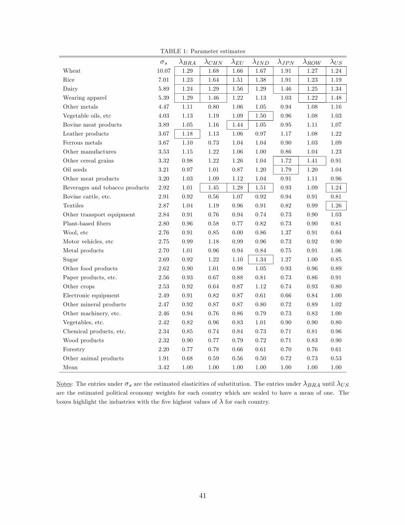
TABLE 1: Parameter estimates

σs λBRA λCHN λEU λIND λJPN λROW λUSWheat 10.07 1.29 1.68 1.66 1.67 1.91 1.27 1.24

Rice 7.01 1.23 1.64 1.51 1.38 1.91 1.23 1.19

Dairy 5.89 1.24 1.29 1.56 1.29 1.46 1.25 1.34

Wearing apparel 5.39 1.29 1.46 1.22 1.13 1.03 1.22 1.48

Other metals 4.47 1.11 0.80 1.06 1.05 0.94 1.08 1.16

Vegetable oils, etc 4.03 1.13 1.19 1.09 1.50 0.96 1.08 1.03

Bovine meat products 3.89 1.05 1.16 1.44 1.05 0.95 1.11 1.07

Leather products 3.67 1.18 1.13 1.06 0.97 1.17 1.08 1.22

Ferrous metals 3.67 1.10 0.73 1.04 1.04 0.90 1.03 1.09

Other manufactures 3.53 1.15 1.22 1.06 1.00 0.86 1.04 1.23

Other cereal grains 3.32 0.98 1.22 1.26 1.04 1.72 1.41 0.91

Oil seeds 3.21 0.97 1.01 0.87 1.20 1.79 1.20 1.04

Other meat products 3.20 1.03 1.09 1.12 1.04 0.91 1.11 0.96

Beverages and tobacco products 2.92 1.01 1.45 1.28 1.51 0.93 1.09 1.24

Bovine cattle, etc. 2.91 0.92 0.56 1.07 0.92 0.94 0.91 0.81

Textiles 2.87 1.04 1.19 0.96 0.91 0.82 0.99 1.26

Other transport equipment 2.84 0.91 0.76 0.94 0.74 0.73 0.90 1.03

Plant-based fibers 2.80 0.96 0.58 0.77 0.82 0.73 0.90 0.81

Wool, etc 2.76 0.91 0.85 0.00 0.86 1.37 0.91 0.64

Motor vehicles, etc 2.75 0.99 1.18 0.99 0.96 0.73 0.92 0.90

Metal products 2.70 1.01 0.96 0.94 0.84 0.75 0.91 1.06

Sugar 2.69 0.92 1.22 1.10 1.34 1.27 1.00 0.85

Other food products 2.62 0.90 1.01 0.98 1.05 0.93 0.96 0.89

Paper products, etc. 2.56 0.93 0.67 0.88 0.81 0.73 0.86 0.91

Other crops 2.53 0.92 0.64 0.87 1.12 0.74 0.93 0.80

Electronic equipment 2.49 0.91 0.82 0.87 0.61 0.66 0.84 1.00

Other mineral products 2.47 0.92 0.87 0.87 0.80 0.72 0.89 1.02

Other machinery, etc. 2.46 0.94 0.76 0.86 0.79 0.73 0.83 1.00

Vegetables, etc. 2.42 0.82 0.96 0.83 1.01 0.90 0.90 0.80

Chemical products, etc. 2.34 0.85 0.74 0.84 0.73 0.71 0.81 0.96

Wood products 2.32 0.90 0.77 0.79 0.72 0.71 0.83 0.90

Forestry 2.20 0.77 0.78 0.66 0.61 0.70 0.76 0.61

Other animal products 1.91 0.68 0.59 0.56 0.50 0.72 0.73 0.53

Mean 3.42 1.00 1.00 1.00 1.00 1.00 1.00 1.00

Notes: The entries under σs are the estimated elasticities of substitution. The entries under λBRA until λUSare the estimated political economy weights for each country which are scaled to have a mean of one. The

boxes highlight the industries with the five highest values of λ for each country.

41

TABLE 2: Effects of 50 percentage point increase in US tariff

General equilibrium effects

∆ US wage ∆ US production (protected) ∆ US production (other)

Chem. 1.45% 5.73% -1.40%

Appar. 0.67% 33.35% -0.97%

Welfare effects

∆ US welfare Terms-of-trade effect Profit shifting effect

Chem. 0.17% 0.34% 0.12%

Appar. -0.14% 0.16% -0.15%

Notes: The entries under "General equilibrium effects" are the percentage change in the US wage normalized

such that the average wage change across all countries is zero (column 1), the percentage change in the quantity

of output in the US chemicals or apparel industry (column 2), and the average of the percentage changes in

the quantity of output in the other US industries (column 3). The entries under "Welfare effects" are the

percentage change in US welfare (column 1), the component due to terms-of-trade effects (column 2), and the

component due to profit shifting effects (column 3). The values in column 2 and 3 do not add up to the value

in column 1 because they are computed using equation (14) which is a linear approximation. Here, all changes

are computed relative to factual tariffs.

42

TABLE 3a: Optimal tariffs without lobbying

∆ gvt. welfare ∆ welfare ∆ wage ∆ profits opt. tariff

own other own other own other own other median

Brazil 1.1% -0.1% 1.1% -0.1% 18.2% -3.0% 0.8% -0.0% 56.1%

China 1.8% -0.6% 1.8% -0.6% 17.6% -2.9% 0.5% -0.1% 59.3%

EU 1.9% -1.0% 1.9% -1.0% 22.5% -3.7% 0.1% -0.2% 61.3%

India 1.7% -0.1% 1.7% -0.1% 8.7% -1.5% 2.7% -0.1% 54.0%

Japan 4.0% -0.3% 4.0% -0.3% 18.6% -3.1% 1.7% -0.1% 59.6%

RoW 2.9% -1.7% 2.9% -1.7% 19.0% -3.2% 1.1% -0.6% 61.5%

US 2.3% -0.9% 2.3% -0.9% 23.8% -4.0% 0.6% -0.1% 60.3%

Mean 2.2% -0.7% 2.2% -0.7% 18.3% -3.1% 1.1% -0.2% 58.9%

TABLE 3b: Optimal tariffs with lobbying

∆ gvt. welfare ∆ welfare ∆ wage ∆ profits opt. tariff

own other own other own other own other median

Brazil 0.9% -0.1% 1.0% -0.1% 18.1% -3.0% 0.3% -0.0% 54.2%

China 1.5% -0.4% 1.5% -0.5% 13.3% -2.2% 0.1% -0.0% 60.7%

EU 2.2% -1.2% 1.7% -1.1% 27.0% -4.5% -0.9% 0.1% 69.0%

India 0.5% -0.0% 0.7% -0.0% 11.4% -1.9% 0.6% -0.0% 49.9%

Japan 2.6% -0.4% 1.0% -0.4% 30.0% -5.0% -1.4% 0.1% 77.5%

RoW 2.9% -1.7% 2.6% -1.8% 21.9% -3.7% -0.1% -0.2% 68.9%

US 2.5% -0.9% 2.1% -0.9% 26.4% -4.4% -0.2% 0.0% 56.4%

Mean 1.9% -0.7% 1.5% -0.7% 21.2% -3.5% -0.2% 0.0% 62.4%

TABLE 3c: Sensitivity of optimal tariffs w.r.t. σs

Without lobbying (all values are means)

σ ∆ gvt. welfare ∆ welfare ∆ wage ∆ profits opt. tariff

mean own other own other own other own other median

3.5 2.2% -0.6% 2.2% -0.6% 17.6% -2.9% 1.1% -0.2% 56.8%

5.0 1.7% -0.4% 1.7% -0.4% 9.1% -1.5% 1.1% -0.2% 34.3%

6.5 1.5% -0.2% 1.5% -0.2% 5.4% -0.9% 1.1% -0.2% 24.6%

With lobbying (all values are means)

σ ∆ gvt. welfare ∆ welfare ∆ wage ∆ profits opt. tariff

mean own other own other own other own other median

3.5 1.8% -0.6% 1.5% -0.6% 20.2% -3.4% -0.2% 0.0% 60.1%

5.0 1.2% -0.4% 0.9% -0.4% 10.5% -1.7% -0.2% 0.0% 35.5%

6.5 1.1% -0.3% 0.7% -0.3% 6.5% -1.1% -0.2% 0.0% 25.6%

Notes: The entries under "gvt. welfare" are the percentage changes in G, the entries under "welfare" are the

percentage changes in W, the entries under "wage" are the percentage changes in w normalized such that the

average wage change across all countries is zero, the entries under "profits" are the percentage changes in total

profits due to changes in industry output, and the entries under "opt. tariff" are the medians of the optimal

tariffs. The entries under "own" are the effects on the tariff imposing country while the entries under "other"

are the averages of the effects on all other countries. The last rows of Tables 3a and 3b report averages. Table

3c reports only such averages.

43

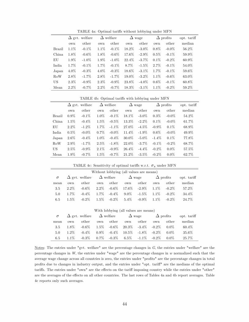
TABLE 4a: Optimal tariffs without lobbying under MFN

∆ gvt. welfare ∆ welfare ∆ wage ∆ profits opt. tariff

own other own other own other own other median

Brazil 1.1% -0.1% 1.1% -0.1% 18.2% -3.0% 0.8% -0.0% 56.2%

China 1.8% -0.6% 1.8% -0.6% 17.6% -2.9% 0.5% -0.1% 59.9%

EU 1.9% -1.0% 1.9% -1.0% 22.4% -3.7% 0.1% -0.2% 60.9%

India 1.7% -0.1% 1.7% -0.1% 8.7% -1.5% 2.7% -0.1% 54.0%

Japan 4.0% -0.3% 4.0% -0.3% 18.6% -3.1% 1.7% -0.1% 59.6%

RoW 2.8% -1.7% 2.8% -1.7% 19.0% -3.2% 1.1% -0.6% 63.0%

US 2.3% -0.9% 2.3% -0.9% 23.8% -4.0% 0.6% -0.1% 60.8%

Mean 2.2% -0.7% 2.2% -0.7% 18.3% -3.1% 1.1% -0.2% 59.2%

TABLE 4b: Optimal tariffs with lobbying under MFN

∆ gvt. welfare ∆ welfare ∆ wage ∆ profits opt. tariff

own other own other own other own other median

Brazil 0.9% -0.1% 1.0% -0.1% 18.1% -3.0% 0.3% -0.0% 54.2%

China 1.5% -0.4% 1.5% -0.5% 13.3% -2.2% 0.1% -0.0% 61.7%

EU 2.2% -1.2% 1.7% -1.1% 27.0% -4.5% -0.9% 0.1% 68.9%

India 0.5% -0.0% 0.7% -0.0% 11.4% -1.9% 0.6% -0.0% 49.9%

Japan 2.6% -0.4% 1.0% -0.4% 30.0% -5.0% -1.4% 0.1% 77.8%

RoW 2.9% -1.7% 2.5% -1.8% 22.0% -3.7% -0.1% -0.2% 68.7%

US 2.5% -0.9% 2.1% -0.9% 26.4% -4.4% -0.2% 0.0% 57.5%

Mean 1.9% -0.7% 1.5% -0.7% 21.2% -3.5% -0.2% 0.0% 62.7%

TABLE 4c: Sensitivity of optimal tariffs w.r.t. σs under MFN

Without lobbying (all values are means)

σ ∆ gvt. welfare ∆ welfare ∆ wage ∆ profits opt. tariff

mean own other own other own other own other median

3.5 2.2% -0.6% 2.2% -0.6% 17.6% -2.9% 1.1% -0.2% 57.2%

5.0 1.7% -0.4% 1.7% -0.4% 9.0% -1.5% 1.1% -0.2% 34.4%

6.5 1.5% -0.2% 1.5% -0.2% 5.4% -0.9% 1.1% -0.2% 24.7%

With lobbying (all values are means)

σ ∆ gvt. welfare ∆ welfare ∆ wage ∆ profits opt. tariff

mean own other own other own other own other median

3.5 1.8% -0.6% 1.5% -0.6% 20.3% -3.4% -0.2% 0.0% 60.4%

5.0 1.2% -0.4% 0.9% -0.4% 10.5% -1.8% -0.2% 0.0% 35.6%

6.5 1.1% -0.3% 0.7% -0.3% 6.5% -1.1% -0.2% 0.0% 25.7%

Notes: The entries under "gvt. welfare" are the percentage changes in G, the entries under "welfare" are the

percentage changes in W, the entries under "wage" are the percentage changes in w normalized such that the

average wage change across all countries is zero, the entries under "profits" are the percentage changes in total

profits due to changes in industry output, and the entries under "opt. tariff" are the medians of the optimal

tariffs. The entries under "own" are the effects on the tariff imposing country while the entries under "other"

are the averages of the effects on all other countries. The last rows of Tables 4a and 4b report averages. Table

4c reports only such averages.

44

TABLE 5a: Nash tariffs without lobbying

∆ gvt. welfare ∆ welfare ∆ wage ∆ profits Nash tariff

Brazil -1.9% -1.9% 1.3% 0.4% 56.4%

China -2.2% -2.2% 0.5% -0.2% 58.6%

EU -2.6% -2.6% 2.7% -0.9% 59.1%

India -2.2% -2.2% -9.3% 1.9% 54.5%

Japan -0.8% -0.8% -0.6% 0.7% 58.5%

RoW -5.0% -5.0% -0.8% -0.6% 59.7%

US -2.2% -2.2% 6.3% -0.3% 59.6%

Mean -2.4% -2.4% 0.0% 0.2% 58.1%

TABLE 5b: Nash tariffs with lobbying

∆ gvt. welfare ∆ welfare ∆ wage ∆ profits Nash tariff

Brazil -2.7% -2.5% -4.6% 0.5% 54.7%

China -3.4% -2.9% -7.1% 0.3% 62.9%

EU -2.2% -2.7% 5.6% -1.2% 69.4%

India -3.6% -3.3% -10.5% 0.8% 54.1%

Japan -1.0% -2.8% 11.4% -1.7% 77.6%

RoW -5.3% -5.6% -1.3% -0.1% 68.5%

US -2.0% -2.4% 6.5% -0.2% 56.6%

Mean -2.9% -3.2% 0.0% -0.2% 63.4%

TABLE 5c: Sensitivity of Nash tariffs w.r.t. σs

Without lobbying (all values are means)

σmean ∆ gvt. welfare ∆ welfare ∆ wage ∆ profits Nash tariff

3.5 -2.3% -2.3% 0.0% 0.2% 56.0%

5.0 -1.0% -1.0% 0.0% 0.3% 34.4%

6.5 -0.3% -0.3% 0.0% 0.2% 25.4%

With lobbying (all values are means)

σmean ∆ gvt. welfare ∆ welfare ∆ wage ∆ profits Nash tariff

3.5 -2.8% -3.0% 0.0% -0.2% 61.2%

5.0 -1.5% -1.7% 0.0% -0.1% 36.2%

6.5 -0.8% -1.1% 0.0% -0.1% 26.4%

Notes: The entries under "gvt. welfare" are the percentage changes in G, the entries under "welfare" are the

percentage changes in W, the entries under "wage" are the percentage changes in w normalized such that the

average wage change across all countries is zero, the entries under "profits" are the percentage changes in total

profits due to changes in industry output, and the entries under "Nash tariff" are the medians of the Nash

tariffs. The last rows of Tables 5a and 5b report averages. Table 5c reports only such averages.

45

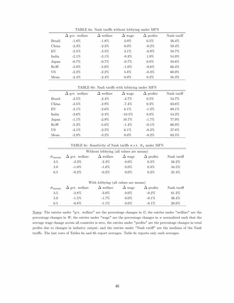
TABLE 6a: Nash tariffs without lobbying under MFN

∆ gvt. welfare ∆ welfare ∆ wage ∆ profits Nash tariff

Brazil -1.8% -1.8% 2.0% 0.5% 56.4%

China -2.3% -2.3% 0.0% -0.2% 59.4%

EU -2.5% -2.5% 3.1% -0.9% 58.7%

India -2.1% -2.1% -9.3% 1.9% 54.9%

Japan -0.7% -0.7% -0.7% 0.8% 58.6%

RoW -5.0% -5.0% -1.0% -0.6% 60.4%

US -2.2% -2.2% 5.8% -0.3% 60.0%

Mean -2.4% -2.4% 0.0% 0.2% 58.3%

TABLE 6b: Nash tariffs with lobbying under MFN

∆ gvt. welfare ∆ welfare ∆ wage ∆ profits Nash tariff

Brazil -2.5% -2.4% -3.7% 0.5% 54.7%

China -3.5% -2.9% -7.4% 0.3% 63.6%

EU -2.1% -2.6% 6.1% -1.2% 69.1%

India -3.6% -3.3% -10.5% 0.8% 54.3%

Japan -1.1% -2.9% 10.7% -1.7% 77.9%

RoW -5.3% -5.6% -1.4% -0.1% 66.9%

US -2.1% -2.5% 6.1% -0.2% 57.8%

Mean -2.9% -3.2% 0.0% -0.2% 63.5%

TABLE 6c: Sensitivity of Nash tariffs w.r.t. σs under MFN

Without lobbying (all values are means)

σmean ∆ gvt. welfare ∆ welfare ∆ wage ∆ profits Nash tariff

3.5 -2.3% -2.3% 0.0% 0.2% 56.2%

5.0 -1.0% -1.0% 0.0% 0.3% 34.5%

6.5 -0.2% -0.2% 0.0% 0.2% 25.4%

With lobbying (all values are means)

σmean ∆ gvt. welfare ∆ welfare ∆ wage ∆ profits Nash tariff

3.5 -2.8% -3.0% 0.0% -0.2% 61.2%

5.0 -1.5% -1.7% 0.0% -0.1% 36.4%

6.5 -0.8% -1.1% 0.0% -0.1% 26.6%

Notes: The entries under "gvt. welfare" are the percentage changes in G, the entries under "welfare" are the

percentage changes in W, the entries under "wage" are the percentage changes in w normalized such that the

average wage change across all countries is zero, the entries under "profits" are the percentage changes in total

profits due to changes in industry output, and the entries under "Nash tariff" are the medians of the Nash

tariffs. The last rows of Tables 6a and 6b report averages. Table 6c reports only such averages.

46

TABLE 7a: Cooperative tariffs without lobbying

∆ gvt. welfare ∆ welfare ∆ wage ∆ profits

Nash Fact. Free Nash Fact. Free Nash Fact. Free Nash Fact. Free

Brazil 3.4% 0.5% 0.03% 3.4% 0.5% 0.03% 9.2% 6.1% 0.1% -0.7% -0.7% 0.0%

China 3.4% 0.5% 0.03% 3.4% 0.5% 0.03% 0.0% 0.2% -0.2% -0.8% -0.9% 0.2%

EU 3.4% 0.5% 0.03% 3.4% 0.5% 0.03% -2.1% 2.7% 0.1% 1.0% 0.3% 0.0%

India 3.4% 0.5% 0.03% 3.4% 0.5% 0.03% 5.8% -4.0% -0.1% -0.9% 1.0% 0.2%

Japan 3.4% 0.5% 0.03% 3.4% 0.5% 0.03% -2.7% -9.4% 0.6% 1.4% 1.8% -0.2%

RoW 3.4% 0.5% 0.03% 3.4% 0.5% 0.03% -6.0% 1.8% -0.2% 0.6% -0.2% 0.3%

US 3.4% 0.5% 0.03% 3.4% 0.5% 0.03% -4.2% 2.8% -0.3% 0.4% 0.3% 0.2%

Mean 3.4% 0.5% 0.03% 3.4% 0.5% 0.03% 0.0% 0.0% 0.0% 0.1% 0.2% 0.1%

TABLE 7b: Cooperative tariffs with lobbying

∆ gvt. welfare ∆ welfare ∆ wage ∆ profits

Nash Fact. Free Nash Fact. Free Nash Fact. Free Nash Fact. Free

Brazil 3.6% 0.5% 0.2% 3.5% 0.5% 0.28% 10.7% 3.3% 1.4% -0.7% -0.1% 0.6%

China 3.6% 0.5% 0.2% 1.0% -1.6% -1.25% -4.7% -8.0% -3.1% -2.3% -2.1% -1.4%

EU 3.6% 0.5% 0.2% 4.0% 0.3% -0.01% -2.7% 0.9% 0.8% 1.4% 0.0% -0.1%India 3.6% 0.5% 0.2% 3.6% 0.8% -0.86% 5.7% 0.6% -0.7% -0.6% 0.2% -0.7%

Japan 3.6% 0.5% 0.2% 4.9% 0.5% -0.44% -0.8% 1.5% 1.0% 1.7% 0.5% -0.5%

RoW 3.6% 0.5% 0.2% 4.2% 0.7% 0.28% -4.7% 1.1% 1.0% 0.4% 0.3% 0.5%

US 3.6% 0.5% 0.2% 4.1% 0.6% 0.15% -3.5% 0.6% -0.4% 1.0% 1.0% 1.0%

Mean 3.6% 0.5% 0.2% 3.6% 0.3% -0.27% 0.0% 0.0% 0.0% 0.1% 0.0% -0.1%

TABLE 7c: Sensitivity of cooperative tariffs w.r.t. σs

Without lobbying (all values are means)

σ ∆ gvt. welfare ∆ welfare ∆ wage ∆ profits

mean Nash Fact. Free Nash Fact. Free Nash Fact. Free Nash Fact. Free

3.5 3.3% 0.5% 0.03% 3.3% 0.5% 0.03% 0.0% 0.0% 0.0% 0.1% 0.2% 0.1%

5.0 2.2% 0.8% 0.01% 2.2% 0.8% 0.01% 0.0% 0.0% 0.0% -0.1% 0.1% 0.1%

6.5 1.7% 1.1% 0.01% 1.7% 1.1% 0.01% 0.0% 0.0% 0.0% -0.2% 0.0% 0.1%

With lobbying (all values are means)

σ ∆ gvt. welfare ∆ welfare ∆ wage ∆ profits

mean Nash Fact. Free Nash Fact. Free Nash Fact. Free Nash Fact. Free

3.5 3.5% 0.5% 0.2% 3.5% 0.3% -0.26% 0.0% 0.0% 0.0% 0.1% 0.0% -0.1%

5.0 2.3% 0.7% 0.3% 2.2% 0.4% -0.29% 0.0% 0.0% 0.0% 0.0% 0.0% 0.1%

6.5 1.8% 1.0% 0.4% 1.7% 0.6% -0.33% 0.0% 0.0% 0.0% 0.1% 0.0% 0.2%

Notes: The entries under "gvt. welfare" are the percentage changes in G, the entries under "welfare" are the

percentage changes in W, the entries under "wage" are the percentage changes in w normalized such that the

average wage change across all countries is zero, and the entries under "profits" are the percentage changes in

total profits due to changes in industry output. The individual columns refer to trade negotiations starting at

Nash tariffs, factual tariffs, and free trade, respectively. The last rows of Tables 7a and 7b report averages.

Table 7c reports only such averages.

47

TABLE 8a: Cooperative tariffs without lobbying under MFN

∆ gvt. welfare ∆ welfare ∆ wage ∆ profits

Nash Fact. Free Nash Fact. Free Nash Fact. Free Nash Fact. Free

Brazil 3.3% 0.3% 0.03% 3.3% 0.3% 0.03% 10.5% 3.3% 0.0% -0.4% -0.5% 0.1%

China 3.3% 0.3% 0.03% 3.3% 0.3% 0.03% -0.3% -0.6% -0.2% -0.5% -0.9% 0.2%

EU 3.3% 0.3% 0.03% 3.3% 0.3% 0.03% -2.3% 1.2% 0.1% 0.9% 0.2% 0.0%

India 3.3% 0.3% 0.03% 3.3% 0.3% 0.03% 5.2% -5.9% -0.2% -0.4% 1.0% 0.3%

Japan 3.3% 0.3% 0.03% 3.3% 0.3% 0.03% -2.9% 0.6% 0.7% 1.2% 0.5% -0.1%

RoW 3.3% 0.3% 0.03% 3.3% 0.3% 0.03% -6.0% 0.5% -0.2% 0.3% -0.1% 0.3%

US 3.3% 0.3% 0.03% 3.3% 0.3% 0.03% -4.2% 0.8% -0.2% 0.3% 0.5% 0.2%

Mean 3.3% 0.3% 0.03% 3.3% 0.3% 0.03% 0.0% 0.0% 0.0% 0.2% 0.1% 0.1%

TABLE 8b: Cooperative tariffs with lobbying under MFN

∆ gvt. welfare ∆ welfare ∆ wage ∆ profits

Nash Fact. Free Nash Fact. Free Nash Fact. Free Nash Fact. Free

Brazil 3.4% 0.3% 0.1% 3.3% 0.3% 0.17% 10.2% 2.5% 0.6% -0.6% -0.2% 0.5%

China 3.4% 0.3% 0.1% 2.2% -0.5% -0.24% -1.0% -5.1% -0.3% -1.1% -1.1% -0.2%

EU 3.4% 0.3% 0.1% 3.8% 0.2% -0.10% -3.6% 0.2% 0.2% 1.2% 0.0% -0.2%

India 3.4% 0.3% 0.1% 3.4% 0.5% -0.30% 4.2% 0.9% -0.2% -0.6% 0.2% -0.3%

Japan 3.4% 0.3% 0.1% 4.5% 0.3% -0.41% -0.7% 0.4% -0.6% 1.3% 0.4% -0.4%

RoW 3.4% 0.3% 0.1% 4.0% 0.5% 0.07% -5.5% 0.4% 0.2% 0.5% 0.2% 0.3%

US 3.4% 0.3% 0.1% 3.8% 0.4% 0.08% -3.5% 0.7% 0.1% 0.7% 0.3% 0.4%

Mean 3.4% 0.3% 0.1% 3.6% 0.2% -0.11% 0.0% 0.0% 0.0% 0.2% 0.0% 0.0%

TABLE 8c: Sensitivity of cooperative tariffs w.r.t. σs under MFN

Without lobbying (all values are means)

σ ∆ gvt. welfare ∆ welfare ∆ wage ∆ profits

mean Nash Fact. Free Nash Fact. Free Nash Fact. Free Nash Fact. Free

3.5 3.2% 0.3% 0.03% 3.2% 0.3% 0.03% 0.0% 0.0% 0.0% 0.2% 0.1% 0.1%

5.0 2.1% 0.6% 0.01% 2.1% 0.6% 0.01% 0.0% 0.0% 0.0% 0.0% 0.0% 0.1%

6.5 1.6% 0.8% 0.01% 1.6% 0.8% 0.01% 0.0% 0.0% 0.0% -0.1% -0.1% 0.1%

With lobbying (all values are means)

σ ∆ gvt. welfare ∆ welfare ∆ wage ∆ profits

mean Nash Fact. Free Nash Fact. Free Nash Fact. Free Nash Fact. Free

3.5 3.3% 0.3% 0.09% 3.5% 0.3% -0.11% 0.0% 0.0% 0.0% 0.2% 0.0% 0.0%

5.0 2.0% 0.4% 0.14% 2.1% 0.3% -0.15% 0.0% 0.0% 0.0% 0.1% -0.1% 0.1%

6.5 1.5% 0.4% 0.20% 1.7% 0.3% -0.20% 0.0% 0.0% 0.0% 0.1% -0.2% 0.1%

Notes: The entries under "gvt. welfare" are the percentage changes in G, the entries under "welfare" are the

percentage changes in W, the entries under "wage" are the percentage changes in w normalized such that the

average wage change across all countries is zero, and the entries under "profits" are the percentage changes in

total profits due to changes in industry output. The individual columns refer to trade negotiations starting at

Nash tariffs, factual tariffs, and free trade, respectively. The last rows of Tables 8a and 8b report averages.

Table 8c reports only such averages.

48

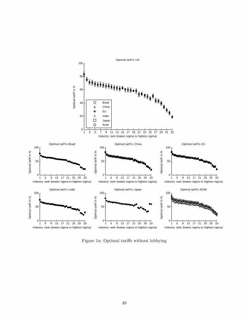
1 5 9 13 17 21 25 29 330

50

100Optimal tarif f s Brazil

Industry  rank (lowest sigma to highest sigma)

Opt

imal

 tar

iff in

 %

1 5 9 13 17 21 25 29 330

50

100Optimal tarif f s China

Industry  rank (lowest sigma to highest sigma)

Opt

imal

 tar

iff in

 %

1 5 9 13 17 21 25 29 330

50

100Optimal tarif f s EU

Industry  rank (lowest sigma to highest sigma)

Opt

imal

 tar

iff in

 %

1 5 9 13 17 21 25 29 330

50

100Optimal tarif f s India

Industry  rank (lowest sigma to highest sigma)

Opt

imal

 tar

iff in

 %

1 5 9 13 17 21 25 29 330

50

100Optimal tarif f s Japan

Industry  rank (lowest sigma to highest sigma)

Opt

imal

 tar

iff in

 %

1 5 9 13 17 21 25 29 330

50

100Optimal tarif f s ROW

Industry  rank (lowest sigma to highest sigma)

Opt

imal

 tar

iff in

 %

1 3 5 7 9 11 13 15 17 19 21 23 25 27 29 31 330

20

40

60

80

100Optimal tarif f s US

Industry  rank (lowest sigma to highest sigma)

Opt

imal

 tar

iff in

 %

BrazilChinaEUIndiaJapanRoW

Figure 1a: Optimal tariffs without lobbying

49

1 5 9 13 17 21 25 29 330

50

100

150

200

250Optimal tarif f s Brazil

Industry  rank (lowest tarif f  to highest tarif f )

Opt

imal

 tar

iff in

 %

1 5 9 13 17 21 25 29 330

50

100

150

200

250Optimal tarif f s China

Industry  rank (lowest tarif f  to highest tarif f )

Opt

imal

 tar

iff in

 %

1 5 9 13 17 21 25 29 330

50

100

150

200

250Optimal tarif f s EU

Industry  rank (lowest tarif f  to highest tarif f )

Opt

imal

 tar

iff in

 %

1 5 9 13 17 21 25 29 330

50

100

150

200

250Optimal tarif f s India

Industry  rank (lowest tarif f  to highest tarif f )

Opt

imal

 tar

iff in

 %

1 5 9 13 17 21 25 29 330

200

400

600

800Optimal tarif f s Japan

Industry  rank (lowest tarif f  to highest tarif f )

Opt

imal

 tar

iff in

 %

1 5 9 13 17 21 25 29 330

50

100

150

200

250Optimal tarif f s RoW

Industry  rank (lowest tarif f  to highest tarif f )

Opt

imal

 tar

iff in

 %

1 5 9 13 17 21 25 29 330

50

100

150

200

250Optimal tarif f s US

Industry  rank (lowest tarif f  to highest tarif f )

Opt

imal

 tar

iff in

 %

DataModel

Figure 1b: Optimal tariffs with lobbying

50

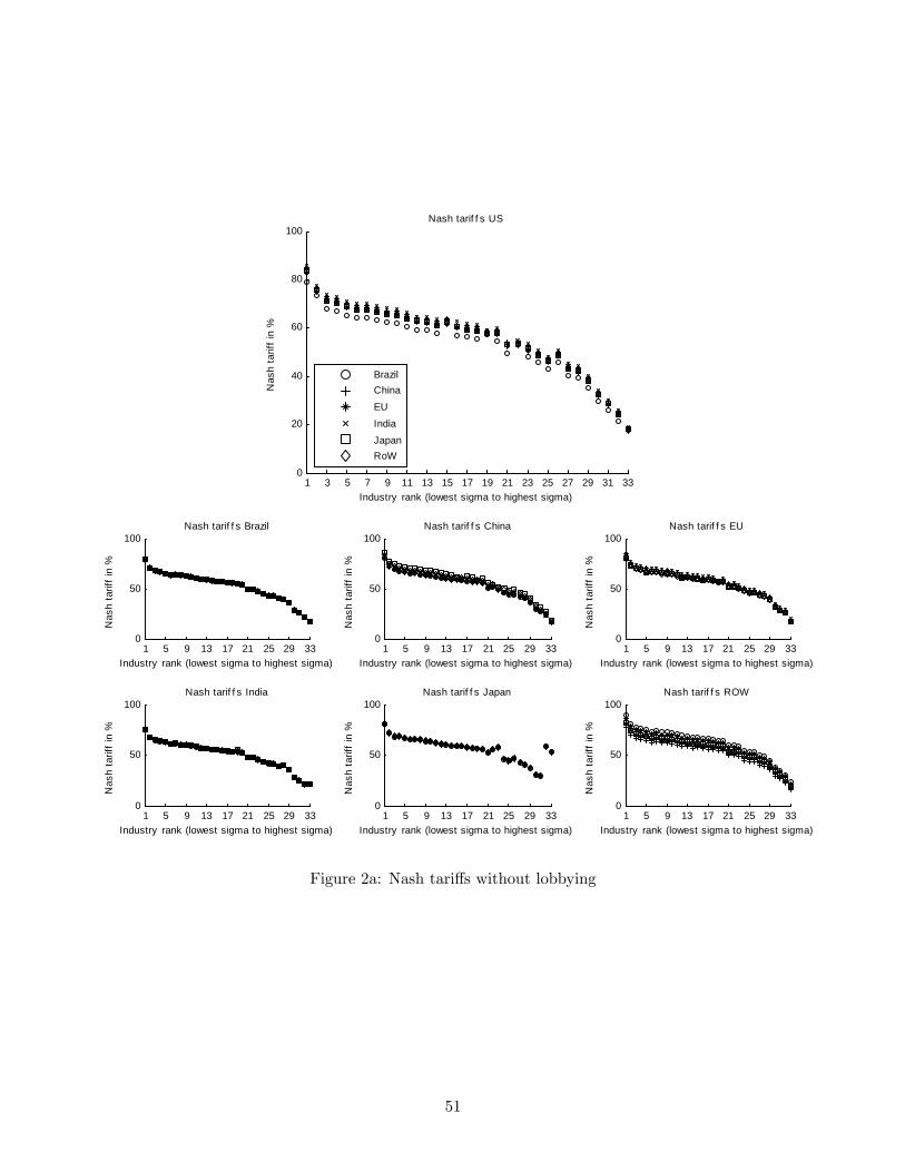
1 5 9 13 17 21 25 29 330

50

100Nash tarif f s Brazil

Industry  rank (lowest sigma to highest sigma)

Nas

h ta

riff 

in %

1 5 9 13 17 21 25 29 330

50

100Nash tarif f s China

Industry  rank (lowest sigma to highest sigma)

Nas

h ta

riff 

in %

1 5 9 13 17 21 25 29 330

50

100Nash tarif f s EU

Industry  rank (lowest sigma to highest sigma)

Nas

h ta

riff 

in %

1 5 9 13 17 21 25 29 330

50

100Nash tarif f s India

Industry  rank (lowest sigma to highest sigma)

Nas

h ta

riff 

in %

1 5 9 13 17 21 25 29 330

50

100Nash tarif f s Japan

Industry  rank (lowest sigma to highest sigma)

Nas

h ta

riff 

in %

1 5 9 13 17 21 25 29 330

50

100Nash tarif f s ROW

Industry  rank (lowest sigma to highest sigma)

Nas

h ta

riff 

in %

1 3 5 7 9 11 13 15 17 19 21 23 25 27 29 31 330

20

40

60

80

100Nash tarif f s US

Industry  rank (lowest sigma to highest sigma)

Nas

h ta

riff 

in %

BrazilChinaEUIndiaJapanRoW

Figure 2a: Nash tariffs without lobbying

51

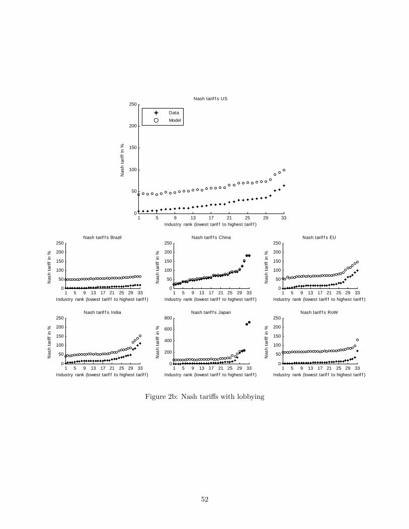
1 5 9 13 17 21 25 29 330

50

100

150

200

250Nash tarif f s Brazil

Industry  rank (lowest tarif f  to highest tarif f )

Nas

h ta

riff 

in %

1 5 9 13 17 21 25 29 330

50

100

150

200

250Nash tarif f s China

Industry  rank (lowest tarif f  to highest tarif f )

Nas

h ta

riff 

in %

1 5 9 13 17 21 25 29 330

50

100

150

200

250Nash tarif f s EU

Industry  rank (lowest tarif f  to highest tarif f )

Nas

h ta

riff 

in %

1 5 9 13 17 21 25 29 330

50

100

150

200

250Nash tarif f s India

Industry  rank (lowest tarif f  to highest tarif f )

Nas

h ta

riff 

in %

1 5 9 13 17 21 25 29 330

200

400

600

800Nash tarif f s Japan

Industry  rank (lowest tarif f  to highest tarif f )

Nas

h ta

riff 

in %

1 5 9 13 17 21 25 29 330

50

100

150

200

250Nash tarif f s RoW

Industry  rank (lowest tarif f  to highest tarif f )

Nas

h ta

riff 

in %

1 5 9 13 17 21 25 29 330

50

100

150

200

250Nash tarif f s US

Industry  rank (lowest tarif f  to highest tarif f )

Nas

h ta

riff 

in %

DataModel

Figure 2b: Nash tariffs with lobbying

52

1 5 9 13 17 21 25 29 33­50

0

50Cooperativ e tarif f s Brazil

Industry  rank (lowest sigma to highest sigma)

Coo

pera

tive 

tarif

f in

 %

1 5 9 13 17 21 25 29 33­50

0

50Cooperativ e tarif f s China

Industry  rank (lowest sigma to highest sigma)

Coo

pera

tive 

tarif

f in

 %

1 5 9 13 17 21 25 29 33­50

0

50Cooperativ e tarif f s EU

Industry  rank (lowest sigma to highest sigma)

Coo

pera

tive 

tarif

f in

 %

1 5 9 13 17 21 25 29 33­50

0

50Cooperativ e tarif f s India

Industry  rank (lowest sigma to highest sigma)

Coo

pera

tive 

tarif

f in

 %

1 5 9 13 17 21 25 29 33­50

0

50Cooperativ e tarif f s Japan

Industry  rank (lowest sigma to highest sigma)

Coo

pera

tive 

tarif

f in

 %

1 5 9 13 17 21 25 29 33­50

0

50Cooperativ e tarif f s ROW

Industry  rank (lowest sigma to highest sigma)

Coo

pera

tive 

tarif

f in

 %

1 3 5 7 9 11 13 15 17 19 21 23 25 27 29 31 33­50

0

50Cooperativ e tarif f s US

Industry  rank (lowest sigma to highest sigma)

Coo

pera

tive 

tarif

f in

 %

BrazilChinaEUIndiaJapanRoW

Figure 3a: Cooperative tariffs without lobbying starting at Nash tariffs

53

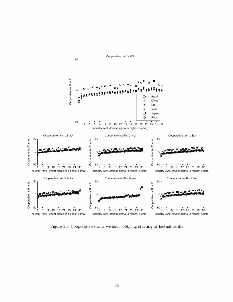
1 5 9 13 17 21 25 29 33­50

0

50Cooperativ e tarif f s Brazil

Industry  rank (lowest sigma to highest sigma)

Coo

pera

tive 

tarif

f in

 %

1 5 9 13 17 21 25 29 33­50

0

50Cooperativ e tarif f s China

Industry  rank (lowest sigma to highest sigma)

Coo

pera

tive 

tarif

f in

 %

1 5 9 13 17 21 25 29 33­50

0

50Cooperativ e tarif f s EU

Industry  rank (lowest sigma to highest sigma)

Coo

pera

tive 

tarif

f in

 %

1 5 9 13 17 21 25 29 33­50

0

50Cooperativ e tarif f s India

Industry  rank (lowest sigma to highest sigma)

Coo

pera

tive 

tarif

f in

 %

1 5 9 13 17 21 25 29 33­50

0

50Cooperativ e tarif f s Japan

Industry  rank (lowest sigma to highest sigma)

Coo

pera

tive 

tarif

f in

 %

1 5 9 13 17 21 25 29 33­50

0

50Cooperativ e tarif f s ROW

Industry  rank (lowest sigma to highest sigma)

Coo

pera

tive 

tarif

f in

 %

1 3 5 7 9 11 13 15 17 19 21 23 25 27 29 31 33­50

0

50Cooperativ e tarif f s US

Industry  rank (lowest sigma to highest sigma)

Coo

pera

tive 

tarif

f in

 %

BrazilChinaEUIndiaJapanRoW

Figure 3b: Cooperative tariffs without lobbying starting at factual tariffs

54

1 5 9 13 17 21 25 29 33­50

0

50Cooperativ e tarif f s Brazil

Industry  rank (lowest sigma to highest sigma)

Coo

pera

tive 

tarif

f in

 %

1 5 9 13 17 21 25 29 33­50

0

50Cooperativ e tarif f s China

Industry  rank (lowest sigma to highest sigma)

Coo

pera

tive 

tarif

f in

 %

1 5 9 13 17 21 25 29 33­50

0

50Cooperativ e tarif f s EU

Industry  rank (lowest sigma to highest sigma)

Coo

pera

tive 

tarif

f in

 %

1 5 9 13 17 21 25 29 33­50

0

50Cooperativ e tarif f s India

Industry  rank (lowest sigma to highest sigma)

Coo

pera

tive 

tarif

f in

 %

1 5 9 13 17 21 25 29 33­50

0

50Cooperativ e tarif f s Japan

Industry  rank (lowest sigma to highest sigma)

Coo

pera

tive 

tarif

f in

 %

1 5 9 13 17 21 25 29 33­50

0

50Cooperativ e tarif f s ROW

Industry  rank (lowest sigma to highest sigma)

Coo

pera

tive 

tarif

f in

 %

1 3 5 7 9 11 13 15 17 19 21 23 25 27 29 31 33­50

0

50Cooperativ e tarif f s US

Industry  rank (lowest sigma to highest sigma)

Coo

pera

tive 

tarif

f in

 %

BrazilChinaEUIndiaJapanRoW

Figure 3c: Cooperative tariffs without lobbying starting at zero tariffs

55

0 20 40 60 80 100­0.5

0

0.5

1

1.5Non­MFN liberalization among EU, Japan, and US

Tarif f  cut relativ e to Nash in %

Avera

ge w

elfare

 cha

nge 

in %

Liberalizing countries

Other countries

0 20 40 60 80 100­1

­0.5

0

0.5

1

1.5Non­MFN liberalization among EU, Japan, and US

Tarif f  cut relativ e to Nash in %

Avera

ge w

age 

chan

ge in

 %

Liberalizing countries

Other countries

0 20 40 60 80 100­1

0

1

2

3

4MFN liberalization among EU, Japan, and US

Tarif f  cut relativ e to Nash in %

Avera

ge w

elfare

 cha

nge 

in %

Liberalizing countries

Other countries

0 20 40 60 80 100­15

­10

­5

0

5

10

15MFN liberalization among EU, Japan, and US

Tarif f  cut relativ e to Nash in %

Avera

ge w

age 

chan

ge in

 %

Liberalizing countries

Other countries

Figure 4: Discriminatory versus nondiscriminatory tariff reductions

56