Trade Credit and Credit Rationing in Canadian Firms

Rose Cunningham International Department

Bank of Canada

September 2006

Abstract

This paper tests the prediction from Burkart and Ellingsen (2004) model that trade credit will be used by medium-wealth and low-wealth firms to help ease bank credit rationing. It does so using a large sample of more than 28,000 Canadian firms. The data supports the main predictions of the model fairly well. The findings indicate that medium-wealth firms substitute trade credit for bank credit, consistent with using it to alleviate bank credit rationing. The low-wealth firms also use trade credit, but it is positively related to their bank credit usage, suggesting those firms are constrained in both bank credit and trade credit markets. I also test other hypotheses arising from the model and the findings suggest that there are very few unconstrained, high-wealth Canadian firms. Moreover, I find low-wealth, declining and distressed firms supply proportionally more trade credit than firms with healthier balance sheets. Although this is somewhat surprising, similar results have been found in other studies, and may simply reflect some exploitation of market power by their customers. JEL Classification Code: G32 *I am grateful for many helpful comments from Ali Dib, Eric Santor, Larry Schembri, seminar participants at the Bank of Canada and an anonymous reviewer at Statistics Canada. I also thank John Baldwin and his staff at Statistics Canada for providing access to the data.

1

1. Introduction

Trade credit refers to credit granted by a supplier to its customers. It is a relatively

expensive form of financing with implicit annual interest rates of over 40 per cent if the firm does

not take advantage of early payment discounts. Yet trade credit is often identified as a very

important source of short term finance for many firms. Why do firms use trade credit instead of

cheaper sources of finance? Why do suppliers provide credit when banks and other financial

institutions exist to do so? Burkart and Ellingsen (2004) develop a theory of trade credit that

addresses these questions by focusing on how the illiquidity of inputs reduces moral hazard risks,

enabling suppliers to provide trade credit when banks would not. Their model explains why firms

of different wealth categories face different degrees of credit rationing and have different trade

credit usage patterns.

I test their model by examining the relationship between trade credit and bank credit for a

large panel of more than 28,000 Canadian firms. To the best of my knowledge, this paper is one of

the first trade credit studies to use panel data with both public and private firms. I use an

endogenous method to split the sample into categories of firms likely to face different degrees of

credit constraints. The findings show that a large portion of Canadian firms appear to be credit

rationed to some extent. The other predictions of the model appear to be fairly consistent with the

data in that medium-wealth firms can use trade credit as a substitute for bank credit, but low-

wealth firms seem to be constrained in both bank credit and trade credit markets.

The most common trade credit terms are simple net terms whereby full payment is

required within a certain period after delivery, often 30 days. A more complex form of trade credit

involves two-part terms such that a discount is offered if payment is made within the discount

period, or full payment is required at the end of the net period. Surveys by Ng, Smith and Smith

2

(1999) and Dun and Bradstreet (1970) indicate that the most common two-part terms are 2/10 net

30. This means a two per cent discount is available if the buyer pays within 10 days of delivery, or

the full amount is required if they pay 11 to 30 days after delivery. Two-part trade credit terms

imply a very high effective annualized interest rate if the purchaser foregoes the discount, equal to

44.6% for 2/10 net 30 terms.1

Trade credit volumes are usually measured by accounts receivable (AR) and accounts

payable (AP). Accounts receivable measure the unpaid claims a firm has against its customers at a

given time, and therefore indicates its supply of trade credit. Accounts payable is a measure of its

usage of trade credit. Trade credit volumes are economically important; for example, in 1998,

accounts receivable for non-financial firms in Canada totalled $202.6 billion, and accounts payables

were $228.6 billion. Therefore accounts receivable were equivalent to 13.4% of total sales revenue

of $1,511 billion in 1998, and the total accounts payable made up 15.1% of sales.2

The next section reviews related theoretical and empirical literature while the third section

describes Burkart and Ellingsen’s model of trade credit in the presence of bank credit rationing and

the resulting testable hypotheses. Section 4 describes the data and summary statistics and section 5

explains the estimation methods. The regression results for the models of trade credit usage,

supply and net trade credit are presented in section 6, and section 7 concludes.

2. Trade Credit Literature

Theories explaining why firms provide or use trade credit focus on several different

motives. There are at least four broad motives for supplying or demanding trade credit: financial

motives, transactions costs, product market information asymmetries, and price discrimination. 1 Assuming a 10 day discount period and 2% discount rate for a $100 purchase, the full price can be viewed as the future value of a loan on the discounted amount for the remaining 20 day period. The implicit annualized interest rate can be found from the expression 98( 1+ i )365/20=100, which gives i=0.446. 2 Statistics Canada. Financial and Taxation Statistics for Enterprises 1998. Cat.61-219-XPB.p.74.

3

Petersen and Rajan (1997) and Burkart et al (2005) provide good reviews of the various theories of

trade credit. The primary focus here is on financial explanations of trade credit.

2.1 Financial Theories of Trade Credit

Financial factors are key motive for both trade credit supply and demand in the literature.

To explain why sellers supply trade credit, many authors assume a comparative advantage that

suppliers have over financial institutions in certain segments of the short-term funds market. One

source of this advantage may be information asymmetries about borrowers’ creditworthiness.

When there are significant information asymmetries between lenders and borrowers, some

potential borrowers may be credit-rationed by banks or other financial institutions.3

Petersen and Rajan (1997) argue that suppliers may have lower monitoring costs and are

thus able to provide trade credit to firms that are bank-finance-constrained. Specifically, suppliers

observe the buyer at regular intervals and may detect changes in the customer’s financial health

sooner than banks or other institutions. Furthermore, the supplier may be better able to enforce

the credit contract with the threat of cutting off supplies. Another source of the supplier’s

comparative advantage may be their superior ability to salvage value from repossessed goods. The

financing advantage suppliers may have allows them to provide liquidity to their customers. The

supplier’s role in providing liquidity was also recognized in early models without asymmetric

information by Emery (1984), Bitros (1979) and Schwartz (1974). Smith (1987) shows that the

terms of trade credit offered by the supplier effectively screen buyers in the presence of

information asymmetries about credit worthiness. Buyers who choose not to pay in the discount

period signal to the supplier that they are a greater credit risk and require additional monitoring.

3 There is a large literature on financing constraints and credit-rationing that arises due to information asymmetries in credit markets. See Hubbard (1998) for a review.

4

Several recent papers formalize the relationship between bank credit rationing and trade

credit due to information asymmetries. Jain (2001) provides a model of trade credit in which

suppliers act as a second layer of financial intermediaries between banks and borrowers due to

their lower monitoring costs. Biais and Gollier (1997) also emphasize the monitoring advantage of

suppliers in a model where banks and suppliers have different signals about the borrower’s credit

worthiness. Trade credit helps alleviate the adverse selection problem for banks by identifying

firms with good investment opportunities.

Burkart and Ellingsen (2004) argue that monitoring cost advantage does not fully explain

the supplier’s advantage over banks. They ask why would banks (specialists in evaluating credit

worthiness) have less information than suppliers, and if they do, why do suppliers not use their

superior information to lend cash rather than inputs? Burkart and Ellingsen develop a model in

which trade credit suppliers can overcome the moral hazard problem of resource diversion by the

borrower better than banks, because inputs are harder to divert than cash, and suppliers have a

monitoring advantage with respect to input use only. Their model predicts that trade credit

increases finance-constrained firms’ access to bank credit, however the poorest firms will be

constrained in both bank credit and trade credit. The Burkart and Ellingsen model is the basis for

the empirical work here and it is described in more detail in the next section.

Wilner (2000) examines trade credit relationships and the exploitation of market power.

Large purchasers of inputs may use trade credit to exploit the trade creditors’ dependence in cases

of financial distress. In his model, large trade debtor firms can extract additional concessions from

a dependent trade creditor in the case of financial distress, but they cannot do so with a trade

creditor that has less financial stake in future sales to the trade debtor. He predicts that large

5

customers with dependent trade credit suppliers will prefer trade credit to bank credit if they are

financially distressed.

2.2 Empirical Findings on Financial Motives for Trade Credit

Existing empirical work on financing models of trade credit supply is somewhat mixed.

Mian and Smith (1992) show that bond-rated firms, which are assumed to have better access to

low-cost financing, provide more trade credit than unrated firms do. Petersen and Rajan (1997) use

age and size as proxies for the suppliers’ access to credit and they find evidence consistent with

finance constraints in that older firms offer more trade credit than younger firms do, although the

coefficients are not economically large. They do find a significant effect when size is used as a

proxy for credit access; large firms offer significantly more trade credit than small firms do.

Petersen and Rajan provide some evidence of finance constraints and trade credit demand using

data on firms’ relationships with their banks. Using the duration of the firm’s relationship with its

primary financial institution as an indicator of the degree to which a firm is credit rationed, they

find firms with shorter banking relationships rely more on trade credit.

One of the most surprising findings of Petersen and Rajan (1997) is that net profits are

negatively related to the amount of trade credit offered, and that even distressed firms with low sales

growth and negative profits offer trade credit. They suggest that this may be a matter of window

dressing, if firms in trouble attempt to keep the sales numbers up by offering trade credit to low

quality customers.

Small firms may not offer as much trade credit even if they also have ready access to funds

from banks or other financial institutions due to economies of scale. Ng, Smith and Smith (1999)

show that large firms may offer more trade credit because they experience scale economies in

providing trade credit. After controlling for size, Ng, Smith and Smith do not find that liquidity is a

6

significant determinant in suppliers’ decisions to offer trade credit. Burkart et al (2005) also find

larger firms tend to offer more trade credit, and that after controlling for size other variables

representing access to bank credit are not significant. They also find that large firms use relatively

less trade credit, but receive more favourable trade credit terms such as longer payment periods,

lower penalties for late payment. These authors also find evidence that the decision to offer trade

credit depends on the moral hazard risk of diversion and nonpayment (consistent with the theory

of Burkart and Ellingsen (2004)), and also on the bargaining power of the trade credit supplier

relative to the buyer.

Demirguc-Kunt and Maksimovic (2001) compare manufacturing firms in 40 countries and

find that the use of trade credit is a complement to bank credit, suggesting that suppliers act as

financial intermediaries between banks and borrowers. Nilsen (2002) argues that firms with

reduced access to other sources of credit use trade credit as a poor substitute for other sources of

financing. He finds evidence supporting this view of trade credit demand and shows that trade

credit is particularly likely to be used as a substitute for other credit during periods of tight

monetary policy.

Although there is a sizable literature on trade credit, there has been very little analysis of

trade credit data from Canada, especially for small firms. Petersen and Rajan (1997) also point out

that panel data analysis is required to further our knowledge of trade credit usage and its

implications. Therefore one contribution of this paper is that it tests trade credit hypotheses on a

large panel dataset of both public and private firms, including many very small firms that may be

the most likely to face credit constraints.

7

3. Theoretical Framework

Burkart and Ellingsen (BE) (2004) model trade credit as a way of overcoming a moral

hazard problems that exists when the entrepreneur’s investment decisions cannot be observed by

lenders, and he may divert some of the resources for private gain. In response to this potential

diversion, lenders ration the entrepreneur’s access to credit.

In the BE model, the entrepreneur’s first best level of investment I* depends on the

relevant equilibrium interest rate, either the bank credit interest rate rBC , or the interest rate implied

by the trade credit terms, rTC > rBC . In deciding how much to invest or divert, the entrepreneur

trades off his return from investing the availabe resources versus his private gain from diverting

them. The resulting incentive constraints determine the equilibrium bank credit limits BC , and

trade credit limits TC . Whether the amount of bank credit or trade credit actually used exhausts

those limits depends on the entrepreneur’s initial funds available for investment, i.e. his wealth. 4

Based on their differing credit limits, entrepreneurs with different wealth levels have

different credit usage and investment behaviour, as summarized in Table 1.

Table 1: Borrowing and Investment Behaviour by Firms in Various Wealth Categories in the Burkart and Ellingsen Model

High-Wealth Medium-Wealth Low-Wealth Bank Credit Usage BC BC< BC BC= BC BC= Trade Credit Usage 0TC = TC TC< TC TC= Investment Level I = I*(rBC) I = I*(r TC) I < I*(rTC)

The model predicts high-wealth entrepreneurs have sufficient internal wealth to finance

their desired investment I*(rBC) and therefore they use less bank credit than their limit,

4 Appendix A provides an overview of their model.

8

BC BC< and do not use trade credit (TC) for financing.5 Medium-wealth entrepreneurs must

borrow to invest I*(rTC). They exhaust their bank credit limit BC BC= , but not their trade credit

limit, TC TC< . Since trade credit is more expensive, investors prefer bank credit, and medium-

wealth entrepreneurs only use trade credit as an imperfect substitute once they reach their bank

credit limit. Entrepreneurs with sufficiently low wealth cannot obtain enough credit to invest

I*(rTC) even when they exhaust both credit lines.

The BE model shows that trade credit helps to mitigate the moral hazard problem and

reduces credit rationing. The availability of trade credit increases aggregate investment since low-

or medium-wealth entrepreneurs are able to invest more than when only bank credit is available.

Testable Hypotheses

Burkart and Ellingsen derive the comparative static effects of changes in the model

parameters on the equilibrium credit limits BC and TC . The authors prove the two credit limits

move together for a given change any of the parameters. An increase in wealth (? ) or product price

(p) increase both BC and TC because they increase the entrepreneur’s residual return from

investment relative to diversion. Similarly, more illiquid inputs (lower ß) or greater creditor security

(lower f ) make diversion less profitable relative to invesment and raise the credit limits. A higher

trade credit interest rate (rTC) decreases the two credit limits because it reduces the payoff to

investment relative to diversion.

The comparative statics, combined with whether the firm exhausts its bank or trade credit

limits, result in different predicted effects from parameter changes for firms in different wealth

categories. Table 2 summarizes the sign predictions and the regression variables I use to test them.

5 Other authors prove that firms may use trade credit for other reasons such as reducing transactions costs, as in Ferris (1981). See Petersen and Rajan (1997) for a review of the literature on motives for using trade credit.

9

Table 2: Sign Predictions for Trade Credit Usage in the Burkart and Ellingsen Model

Model Parameter Regression Proxy Predicted Change in Trade Credit Use from an Increase in Explantory Variable

Low-Wealth Medium-Wealth High-Wealth

Bank Credit (BC) LOANS/SALES + - 0 Input Iliquidity (-ß) CAPEX/SALES + 0 0 Wealth (? ) PROFIT/SALES + - 0 Creditor Security (-f ) COVRATIO + - 0

Revenue (P(Q)) SALES SHOCK + ? 0 Trade Credit Cost (rTC) industry dummy variables - ? 0

The trade credit and bank credit limits are both binding for low-wealth entrepreneurs.

Low-wealth entrpreneurs are also predicted to have a positive relationship between bank credit and

trade credit because any change to one credit limit affects the other credit in the same direction.

Thus one of the main predictions of the model is that, for low-wealth firms, trade credit and bank

credit are complements. The other sign preditions all follow from the comparative statics for trade

credit limits described above.

The predictions for the medium-wealth group are more complex. These entrepreneurs are

at their bank credit limit, but they have not exhausted the trade credit available to them. Therefore,

they compensate for reductions in bank credit by increasing their use of trade credit. This credit

substitution effect for medium-wealth firms is a key prediction to test in this study. Burkart and

Ellingsen also predict that medium-wealth entrepreneurs trade credit usage is decreasing in wealth

and increasing in creditor vulnerability (since these variables both change BC ). The authors show

that input liquidity does not affect how much trade credit the medium-wealth entrepreneurs use.

The sign predictions for product price or the trade credit interest rate are ambiguous because

changes in those parameters have opposing effects on trade credit usage.

10

High-wealth entrepreneurs do not use trade credit for financing in Burkart and Ellingsen’s

model, so there are no significant relationships predicted between trade credit usage and the

explanatory variables for the high-wealth group.

The Burkart and Ellingsen model focuses primarily on trade credit usage. With respect to a

firm’s decision to offer trade credit, the authors predict that bank-credit-constrained entrepreneurs

will offer trade credit up to the point where an extra dollar of trade credit given earns as high a

return an extra dollar invested. BE argue that trade credit claims provide collateral for suppliers

because they are illiquid, so the entrepreneur can then borrow against those illiquid trade credit

claims (accounts receivables) and obtain more bank credit. Therefore many firms, even low-wealth

firms, will simultaneously give and take trade credit in the BE model, and there is a positive

relationship between trade credit supplied and bank credit.

4. Data Description and Summary Statistics

I use annual, unpublished microdata on firms in Statistics Canada’s Financial and Taxation

Statistics for Enterprises (FTSE) dataset. The FTSE contains balance sheet and income statement

data. The data cover an 11-year period from 1988 to 1998. Some firms have fewer than 11 years of

data, so the panel is unbalanced.

Trade credit volumes are available from the customers’ perspective (accounts payable), and

from the suppliers’ perspective (accounts receivable), but unfortunately the dataset does not have

information on trade credit terms. However, a key advantage of the FTSE microdata is that it

includes both public and private firms, including some very small firms which may be most likely

to face credit constraints. Another advantage of the FTSE database is its size. I use only a subset of

the observations where sales growth is non-negative (since that is the criteria used to identify firms

11

with good investment opportunities) but this still leaves 72,291 observations on 28,749 firms.

Appendix B provides further details on the data and variable construction.

Over the sample period, aggregate FTSE data show that nominal total sales of goods and

services by Canadian non-financial firms increased from $991 billion in 1988 to $1,510 billion in

1998.6 By comparison, the sample firms’ weighted sales total $496 billion in 1988 and $613.5 billion

in 1998. Over the 11 year period studied, the sample firms’ weighted sales account for 36.8 per

cent to 59.6 per cent of the aggregate sales for the Canadian non-financial sector.

Table 3 presents summary statistics for the variables and observations used in the main

regression analyses. Perhaps the most striking feature of the data is that the mean and median

values are very different for most variables, often by a factor of ten or more. This reflects the fact

that the population of Canadian firms consists of many small firms and a few large firms. The

means are strongly influenced by the large firms and are usually much higher than the median

values. For accounts payable, which measures trade credit utilization, the mean is $6.5 million but

the median is only $327 thousand in 1997 Canadian dollars. The mean accounts receivables are

somewhat larger than accounts payable at $7.3 million, but the median value is only $362 thousand.

Net trade balances are quite small but similarly skewed. Consistent with the reported importance of

trade credit as a source of finance for small firms, accounts payable and accounts recievable are

comprable in size to the bank loan amounts for this sample of firms. Capital expenditures and

profits are considerably smaller, with mean values of $3.8 million and $2.2 million respectively.

Sales average $65 million with a median value of $5 million.

Scaling the variables by sales gives the proportion of trade credit used or supplied by the

firm. The ratios are less skewed since the medians and means are fairly similar for most variables.

6 Statistics Canada. Financial and Taxations Statistics for Enterprises Cat. No.61-219XPB, various years.

12

The means and medians for AP/SALES are 0.094 and 0.073 respectively, and for AR/SALES

the mean and median values are 0.109 to 0.091. On balance, the net trade credit to sales is slightly

positive for these firms with nonnegative sales growth. The Canadian data here seem broadly

consistent with findings from Petersen and Rajan (1997) who study U.S. trade credit data from

1987. The U.S. firms in their sample have mean AP/SALES of 0.044 for small firms and 0.116 for

large firms; and they find mean AR/SALES of 0.073 for small firms, and 0.185 for large firms.

Also Burkart et al (2005) find AR/SALES of 0.10 in their 1998 dataset of small U.S. firms.

Table 3: Summary Statistics for Canadian Firms 1988-1998 thousands of 1997 Canadian dollars (72,291 observations, 28,749 firms)

Mean Median Std. Dev.

ACCTS. PAYABLE (AP) 6468.81 327.00 51105.44 ACCTS. RECEIVABLE(AR) 7277.39 362.00 55377.60

NET TC (AR-AP) 808.57 16.00 29734.52

LOANS 7733.90 204.84 86894.46

CAPITAL EXPENDITURE 3783.41 67.26 40518.97

PROFIT 2221.49 73.28 41457.92

SALES 64967.17 4999.00 460117.80

AP/SALES 0.094 0.073 0.092 AR/SALES 0.109 0.091 0.106

NET TC/SALES 0.016 0.009 0.112

LOANS/SALES 0.085 0.012 0.169

CAPITAL EXP./SALES 0.046 0.014 0.081

PROFIT/SALES 0.029 0.018 0.499

COVERAGE RATIO 25.07 2.76 336.52

SALES GROWTH (Y/Y%) 125.23 12.43 10647.94

13

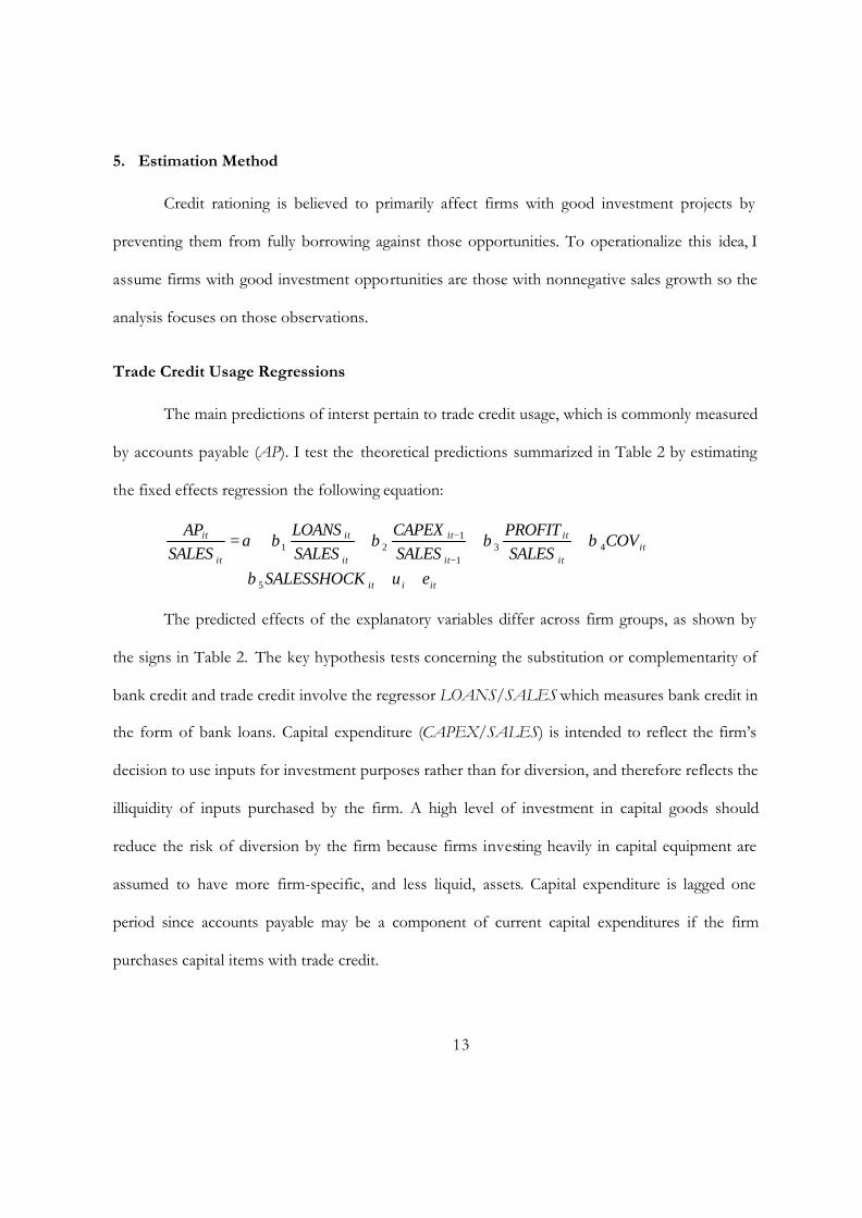
5. Estimation Method

Credit rationing is believed to primarily affect firms with good investment projects by

preventing them from fully borrowing against those opportunities. To operationalize this idea, I

assume firms with good investment opportunities are those with nonnegative sales growth so the

analysis focuses on those observations.

Trade Credit Usage Regressions

The main predictions of interst pertain to trade credit usage, which is commonly measured

by accounts payable (AP). I test the theoretical predictions summarized in Table 2 by estimating

the fixed effects regression the following equation:

itiit

itit

it

it

it

it

it

it

it

euSALESSHOCK

COVSALES

PROFITSALESCAPEX

SALESLOANS

SALESAP

+++

++++=−

−

5

431

121

β

ββββα

The predicted effects of the explanatory variables differ across firm groups, as shown by

the signs in Table 2. The key hypothesis tests concerning the substitution or complementarity of

bank credit and trade credit involve the regressor LOANS/SALES which measures bank credit in

the form of bank loans. Capital expenditure (CAPEX/SALES) is intended to reflect the firm’s

decision to use inputs for investment purposes rather than for diversion, and therefore reflects the

illiquidity of inputs purchased by the firm. A high level of investment in capital goods should

reduce the risk of diversion by the firm because firms investing heavily in capital equipment are

assumed to have more firm-specific, and less liquid, assets. Capital expenditure is lagged one

period since accounts payable may be a component of current capital expenditures if the firm

purchases capital items with trade credit.

14

Funds available for investing, called wealth in the BE model, is proxied by different

variables in the trade credit literature: assets, bank credit and profits. Bank credit provides the key

test described above, and we also operationalize available funds by including a profit measure, net

income before tax, denoted PROFIT. The interest coverage ratio (COV) is a common measure of

credit quality and is included in the regression as a proxy for creditor security. A higher coverage

ratio improves the likelihood of repayment and reduces creditor vulnerability.

The SALESSHOCK variable controls for unexpected changes in demand conditions faced

by the firm, which is meant to correspond to changes in output prices (p) in the BE model. The

SALESSHOCK variable consists of the residuals from an auxiliary OLS regression of sales on a

full set of industry and year dummy variables. The predictions from the auxiliary regression

produces the expected sales for a firm in a given year and industry, and the residuals capture

demand shocks faced by individual firms. I do not have a measure of trade credit financing cost in

the regression; however, Ng, Smith and Smith (1999) and others have observed that there is very

little variation in trade credit terms over time, but considerable cross-industry variation. I include

time and industry dummy variables in the regressions to control for these effects.

Trade Credit Supplied

To analyze trade credit supply behaviour the dependent variable in the regression is

AR/SALES. The theoretical model predicts that a bank-credit-constrained firm will offer trade

credit as long as the trade credit extended earns as high a return as their investment project. I

expect that firms with slow sales growth probably have fewer good investment opportunities than

faster-growing firms, so I add an explanatory variable, GROWTH, to the regression equation for

trade credit supplied. The GROWTH variable is expected to have a negative coefficient.

15

BE argue that since AR claims are illiquid, they can be used as collateral to obtain more

bank loans, and so there should be a positive relationship between trade credit supplied and

LOANS/SALES. A positive relationship may also occur if the causality runs from bank credit to

trade credit because firms with greater access to bank credit just pass it on to their customers. The

other variables should have the same signs as predicted for the AP regressions since the firm still

faces a diversion decision – whether to divert available bank credit or use it to finance accounts

receivable (trade credit lending).

Net Trade Credit

Although the BE model does not explicitly deal with net trade credit (AR-AP), one can

interpret the main BE results concerning the substitution or complementarity of bank and trade

credit as affecting net trade credit positions. The entrepreneur’s aggregate credit limit is BC + TC .

Now, consider the effects of a reduction in the bank credit limit. Medium-wealth firms can

increase their use of trade credit to make up for the decrease in bank credit. They may also choose

to decrease the credit they supply, AR, or perhaps to preserve good relationships with their

customers they keep AR the same. Whether AR remains fixed or is decreased, net trade credit

(AR-AP) will decrease as long as AP increases by more than AR decreases. So for medium-wealth

firms, I expect a positive coefficient on the bank loans variable in the net trade credit regression.

For low-wealth firms, bank credit reductions decrease trade credit usage AP and may also

lead to reduced AR. A reduction in bank credit increases net trade credit (AR-AP) for low-wealth

firms if AR remains constant or is reduced by less than AP. If AR and AP fall by the same amount

in response to lower bank credit, then net trade credit is unchanged. Therefore, I expect that low-

wealth firms’ net trade credit is more negatively related or unrelated to the bank credit variable.

16

Sample Splitting and Estimating Wealth Category Thresholds

As the theory predicts different behaviour for different categories based on their access to

investment funds (wealth), the regression models are estimated for each wealth-group by adding

dummy variables for low and medium-wealth categories and interacting these dummy variables

with the other explanatory variables. To define the high, medium and low wealth categories, one

needs to find a lower and upper threshold that distinguishes low-wealth from medium-wealth and

medium-wealth from high-wealth. Previous studies on credit rationing often use arbitrarily

assigned thresholds, such as the median or other quartiles. Since the sample here has so many small

firms and appears to be quite skewed with respect profits and other variables, there is likely to be a

large proportion of credit-constrained, low-wealth firms. Nevertheless it is not obvious where the

boundaries between wealth groups are. Therefore it seems appropriate to try to find the wealth

thresholds using an endogenous method.

I follow the approach recommended by Hansen (2000) to find endogenous thresholds.

First, to find the low -wealth threshold, I define a LOW dummy variable which equals one if

PROFIT is below a given value, which is allowed to range from -$50 thousand to $174 thousand

1997 dollars. This range corresponds to about the 10th and 75 th percentiles of the profit variable,

giving a large window around the median, a natural starting point. The LOW dummy and

interactions of LOW with the other five main regressors are added to the basic regression model

which is then is estimated separately for each value of PROFIT in the range. The sum of squared

residuals from each regression are then compared and the low-wealth threshold selected is the

value of PROFIT that minimizes the sum of the squared residuals. This process yielded a lower

profit threshold of $60 thousand, equal to about the 55th percentile of PROFIT. Low-wealth firms

are therefore defined as those with profit less than $60 thousand in 1997 dollars.

17

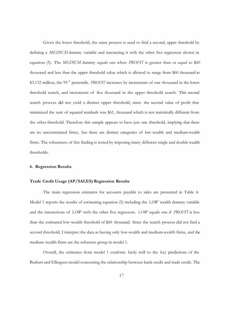
Given the lower threshold, the same process is used to find a second, upper threshold by

defining a MEDIUM dummy variable and interacting it with the other five regressors shown in

equation (5). The MEDIUM dummy equals one when PROFIT is greater than or equal to $60

thousand and less than the upper threshold value which is allowed to range from $60 thousand to

$3.132 million, the 95 th percentile. PROFIT increases by increments of one thousand in the lower

threshold search, and increments of five thousand in the upper threshold search. This second

search process did not yield a distinct upper threshold, since the second value of profit that

minimized the sum of squared residuals was $61, thousand which is not statistically different from

the other threshold. Therefore this sample appears to have just one threshold, implying that there

are no unconstrained firms, but there are distinct categories of low-wealth and medium-wealth

firms. The robustness of this finding is tested by imposing many different single and double wealth

thresholds.

6. Regression Results

Trade Credit Usage (AP/SALES) Regression Results

The main regression estimates for accounts payable to sales are presented in Table 4.

Model 1 reports the results of estimating equation (5) including the LOW wealth dummy variable

and the interactions of LOW with the other five regressors. LOW equals one if PROFIT is less

than the estimated low -wealth threshold of $60 thousand. Since the search process did not find a

second threshold, I interpret the data as having only low-wealth and medium-wealth firms, and the

medium-wealth firms are the reference group in model 1.

Overall, the estimates from model 1 conform fairly well to the key predictions of the

Burkart and Ellingsen model concerning the relationship between bank credit and trade credit. The

18

medium-wealth firms do seem to substitute trade credit for bank credit since the coefficient on

LOANS/SALES is negative and signficantly different from zero at the one per cent level. The

low-wealth firms have a positive and significant coefficient on LOANS/SALES, implying that for

them, bank credit and trade credit are complements rather than substitutes, consistent with the BE

theory. All the other variables in model 1 have the predicted signs for the medium-wealth firms,

except PROFIT/SALES for which the sign is contrary to the predictions for both low- and

medium-wealth firms. The contrary signs on the PROFIT/SALES variable suggests that the

theory’s cyclical implications do not match the data well, however, neither coefficient is

significantly different from zero at the five per cent level. The predictions for variables other than

bank loans hold up less well for the low-wealth firms. Three variables, LOWxPROFIT/SALES,

LOWxCOV and LOWxSALESSHOCK, have signs contrary to predictions, but they are also very

small and not significant at the five per cent level.

Although the estimated relationships between bank credit and trade credit are statistically

significant, they do not appear to be economically large. For the average medium-wealth firm in

the sample, a one standard deviation increase in its bank credit to sales ratio (from 0.085 to 0.245)

results in a decrease in its AP/SALES ratio of just 0.003, reducing the average trade credit usage

ratio from 0.094 to 0.091. For low-wealth firms, the estimated bank loans coefficient of 0.0246 (-

0.0181 + 0.0327) implies that a one standard deviation increase in LOANS/SALES of 0.169

would increase AP/SALES by just 0.004, raising the ratio to 0.098 for the average firm.

Model 1 relies on an estimated threshold to split the sample into low- and medium-wealth

firms. To test the robustness this threshold, I also estimate the model using the 25th, 35th, 45th 50th,

65th, 75th, 85th and 95 th percentiles of PROFIT as threshold to define the LOW dummy variable.

The results are qualitatively the same as reported for model 1 in Table 4. The coefficient on

19

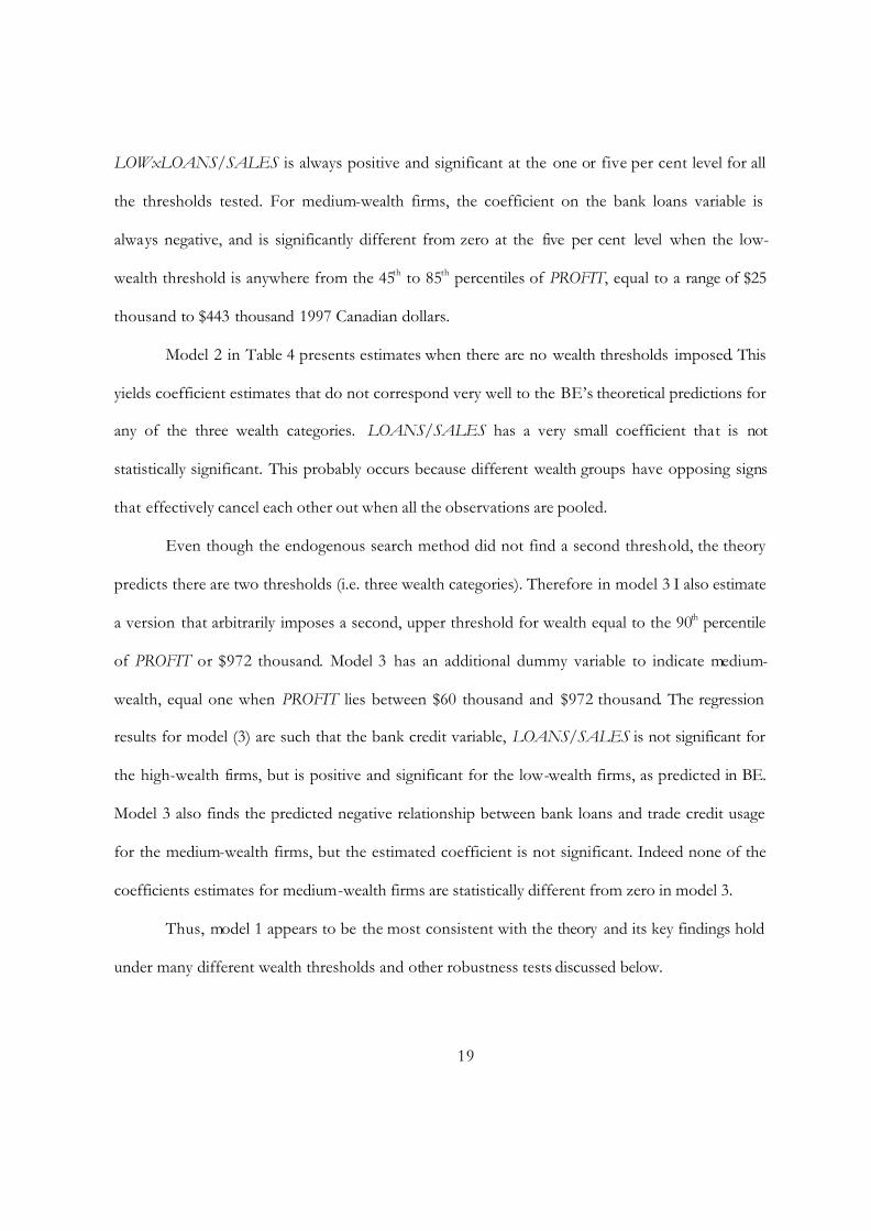
LOWxLOANS/SALES is always positive and significant at the one or five per cent level for all

the thresholds tested. For medium-wealth firms, the coefficient on the bank loans variable is

always negative, and is significantly different from zero at the five per cent level when the low-

wealth threshold is anywhere from the 45th to 85th percentiles of PROFIT, equal to a range of $25

thousand to $443 thousand 1997 Canadian dollars.

Model 2 in Table 4 presents estimates when there are no wealth thresholds imposed. This

yields coefficient estimates that do not correspond very well to the BE’s theoretical predictions for

any of the three wealth categories. LOANS/SALES has a very small coefficient that is not

statistically significant. This probably occurs because different wealth groups have opposing signs

that effectively cancel each other out when all the observations are pooled.

Even though the endogenous search method did not find a second threshold, the theory

predicts there are two thresholds (i.e. three wealth categories). Therefore in model 3 I also estimate

a version that arbitrarily imposes a second, upper threshold for wealth equal to the 90th percentile

of PROFIT or $972 thousand. Model 3 has an additional dummy variable to indicate medium-

wealth, equal one when PROFIT lies between $60 thousand and $972 thousand. The regression

results for model (3) are such that the bank credit variable, LOANS/SALES is not significant for

the high-wealth firms, but is positive and significant for the low-wealth firms, as predicted in BE.

Model 3 also finds the predicted negative relationship between bank loans and trade credit usage

for the medium-wealth firms, but the estimated coefficient is not significant. Indeed none of the

coefficients estimates for medium-wealth firms are statistically different from zero in model 3.

Thus, model 1 appears to be the most consistent with the theory and its key findings hold

under many different wealth thresholds and other robustness tests discussed below.

20

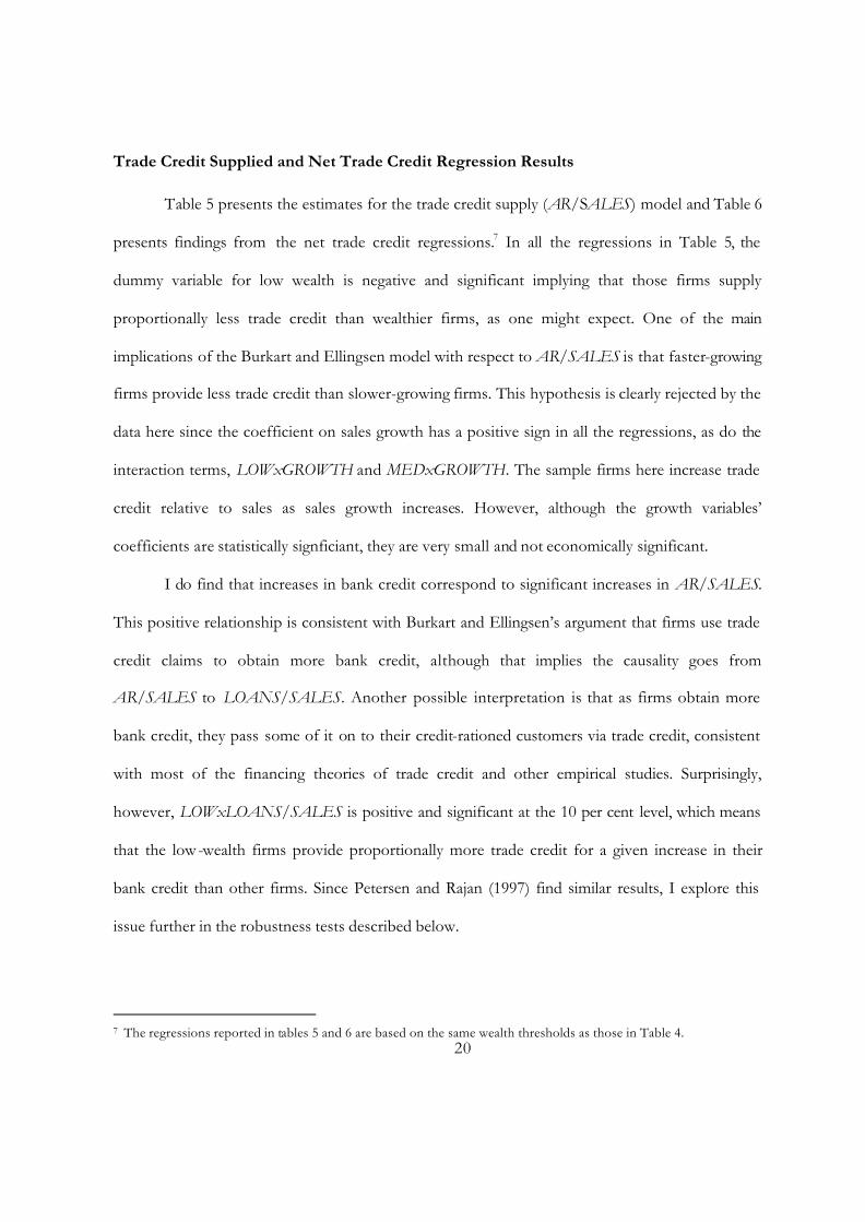
Trade Credit Supplied and Net Trade Credit Regression Results

Table 5 presents the estimates for the trade credit supply (AR/SALES) model and Table 6

presents findings from the net trade credit regressions.7 In all the regressions in Table 5, the

dummy variable for low wealth is negative and significant implying that those firms supply

proportionally less trade credit than wealthier firms, as one might expect. One of the main

implications of the Burkart and Ellingsen model with respect to AR/SALES is that faster-growing

firms provide less trade credit than slower-growing firms. This hypothesis is clearly rejected by the

data here since the coefficient on sales growth has a positive sign in all the regressions, as do the

interaction terms, LOWxGROWTH and MEDxGROWTH. The sample firms here increase trade

credit relative to sales as sales growth increases. However, although the growth variables’

coefficients are statistically signficiant, they are very small and not economically significant.

I do find that increases in bank credit correspond to significant increases in AR/SALES.

This positive relationship is consistent with Burkart and Ellingsen’s argument that firms use trade

credit claims to obtain more bank credit, although that implies the causality goes from

AR/SALES to LOANS/SALES. Another possible interpretation is that as firms obtain more

bank credit, they pass some of it on to their credit-rationed customers via trade credit, consistent

with most of the financing theories of trade credit and other empirical studies. Surprisingly,

however, LOWxLOANS/SALES is positive and significant at the 10 per cent level, which means

that the low -wealth firms provide proportionally more trade credit for a given increase in their

bank credit than other firms. Since Petersen and Rajan (1997) find similar results, I explore this

issue further in the robustness tests described below.

7 The regressions reported in tables 5 and 6 are based on the same wealth thresholds as those in Table 4.

21

Table 4: Trade Credit Usage Regression Results fixed effects regression (72,291 observations 28,749 firms)

(1) (2) (3) Dependent Variable is AP/SALES

Low-Wealth Threshold

No Wealth Thresholds

Low- and High-Wealth Thresholds

Coeff. t-stat. Coeff. t-stat. Coeff. t-stat.

LOANS/SALES -0.0181*** -2.51 9.66e05 0.02 -0.0144 -1.51 CAPEX t-1/SALES t-1 5.26e05 0.67 2.18e04 0.92 0.0029 0.54 PROFIT/SALES 0.0013 1.51 -2.11e05 -0.65 1.09e04 1.01 COV -2.62e06** -2.23 -3.49e06** -2.32 -2.54e06** -2.20 SALES SHOCK -1.31e08*** -4.28 -1.32e08*** -4.22 -1.30e08*** -4.33 LOW WEALTH DUMMY 0.0017 1.55 0.0086*** 4.30 LOWxLOANS/SALES 0.0327*** 4.45 0.0278*** 2.81 LOWxCAPEXt-1/SALES t-1 5.96e05 0.57 -0.0022 -0.41 LOWxPROFIT/SALES -1.93e05* -1.94 -0.0016 -1.42 LOWx COV -3.06e05 -1.56 -3.09e05 -1.56 LOW xSALES SHOCK -1.61e09 -0.85 -3.38e09* -1.79 MED. WEALTH DUMMY

0.0076*** 3.88

MEDx LOANS/SALES -0.0071 -0.63 MEDxCAPEXt-1/SALES t-1 -0.0029 -0.54 MEDxPROFIT/SALES 0.0016 1.06 MEDxCOV 1.30e05 0.81 MEDxSALES SHOCK 1.24e09 0.10 Adjusted R-squared 0.6550 0.6566 0.6584

Note: Statistical significance is indicated by ***, **, and * for 1-per cent, 5-per cent and 10 -per cent levels, respectively. All regressions use White’s robust standard errors and incude a constant and year dummy variables. The low-wealth threshold to identify low wealth firms was found by estimating model (2) allowing PROFIT to range from (-50 to 174) and selecting the profit value that minimized the sum of squared residuals. This method defined low wealth firms are those with PROFIT<$60,000 (about the 55th percentile). The same method found no second upper threshold to define high-wealth firms. Models (2) and (3) provide robustness tests of the thresholds. Model (3) imposes the 90th percentile of PROFIT, $972,000 to define medium wealth firms as those with 60=PROFIT<972. See text for more detail on method and robustness tests.

22

Table 5: Trade Credit Supplied Regression Results fixed effects regressions (72,291 observations 28,749 firms)

(1) (2) (3) Dependent Variable is AR/SALES

Low-Wealth Threshold

No Wealth Thresholds

Low- and High-Wealth Thresholds

Coeff. t-stat. Coeff. t-stat. Coeff. t-stat.

LOANS/SALES 0.0457*** 7.50 0.0508*** 10.41 0.0402*** 4.45 CAPEX t-1/SALES t-1 1.88e04*** 3.65 2.46e04*** 2.80 0.0054* 1.66 PROFIT/SALES 7.28e06 0.16 -1.89e06 -0.94 -3.63e05 -0.79 COV -1.41e06 -1.00 -2.39e06 -1.41 -1.30e06 -0.92 SALES SHOCK -1.63e08*** -3.89 -1.58e08*** -3.78 -1.63e08*** -3.88 GROWTH 7.21e07*** 6.53 7.23e07*** 6.52 8.28e07*** 33.66 LOW WEALTH DUMMY -0.0056*** -5.73 -0.0053*** -2.94 LOWxLOANS/SALES 0.0117* 1.80 0.0180* 1.86 LOWxCAPEXt-1/SALES t-1 2.56e04 0.99 -0.0050 -1.52 LOWxPROFIT/SALES -3.94e05 -0.77 5.19e06 0.10 LOWx COV -3.53e05* -1.88 -3.51e05* -1.91 LOW xSALES SHOCK -2.98e09** -1.97 -3.21e09** -2.07 LOWxGROWTH 1.59e06* 1.64 1.64e06* 1.76 MED. WEALTH DUMMY

-0.0004 -0.22

MEDx LOANS/SALES 0.0095 0.94 MEDxCAPEXt-1/SALES t-1 -0.0053 -1.61 MEDxPROFIT/SALES 0.0018 1.44 MEDxCOV -3.03e06 -0.20 MEDxSALES SHOCK -1.93e09 -0.16 MEDxGROWTH -6.84e07*** -2.91 Adjusted R-squared 0.7565 0.7572 0.7573 Note: Wealth thresholds are the same as those used for AP/SALES regressions. See notes to Table 4.

23

The BE framework can also generate testable predictions for net trade credit. Specifically,

the bank credit variable is expected to have a positive influence on the net trade credit to sales ratio

for medium-wealth firms, and to have a negative or zero coefficient for the low-wealth firms. The

regression results in Table 6 provide considerable support for this prediction, since the coefficient

on LOANS/SALES is positive and highly significant, consistent with the prediction for medium-

wealth firms. Also in model 1, the coefficient for LOWxLOANS/SALES is negative and

significant, so there is a significant difference from the other firms. This difference implies that

medium-wealth firms increase net trade credit more for a given increase in bank credit than low-

wealth firm do. Neverthess, the estimated coefficient for bank loans for the low wealth firms is

0.0430, contrary to the prediction of a negative or zero coefficient. The trade credit supply and net

trade credit regressions provide some additional support for the theoretical model, especially for

medium-wealth firms.

6.3 Robustness Tests

Although there are no explicit predictions about the trade credit behaviour of firms that

may be financially distressed in the Burkart and Ellingsen model, Petersen and Rajan (1997) find

that distressed firms offer proportionally more trade credit than other firms. I find something

similar for growing firms with low-wealth in Table 5. To compare my findings more directly with

Petersen and Rajan, I also estimate the basic model (no wealth thresholds) for firms with negative

sales growth and distressed firms. Distressed firms are defined as those with negative sales growth

and negative profit. These results are reported in Table 7. In columns 1 and 3, trade credit usage

increases as bank credit increases for both the declining and distressed firms. This is not surprising

since declining and distressed firms are likely to be constrained in their access to both bank and

24

trade credit, leading to a complementary relationship between the two types of credit as in the

earlier findings for low -wealth firms.

With respect to trade credit supplied, the AR/SALES regressions indicate that both

declining and distressed firms increase their trade credit supplied when their bank loans increase.

This finding is consistent with Petersen and Rajan but is surprising, especially for the distressed

firms. Firms that are in trouble might decrease the trade credit they provide if bank credit declines,

but one would not expect them to increase their supply of trade credit if their access to bank credit

improved. Wilner (2000) provides a potential explanation. Customers of distressed suppliers may

have high market power such that dependent trade creditors are required by their large customers

to provide credit even in periods of financial distress. A financially distressed supplier may be

distressed because its largest customers are distressed. Wilner predicts that large, financially

distressed customers prefer trade credit from a dependent supplier to credit from sources that are

less dependent on them for future profits. The sample data here may be picking up on the kind of

exploitation of buyers’ market power predicted in Wilner’s model. In empirical tests on trade credit

terms (rather than the volumes studied) Burkart et al (2005) also find evidence that buyers exert

market power over trade credit suppliers such that buyers with many suppliers receive more

generous trade credit concessions such as early payment discountrs and longer payment periods.

25

Table 6: Net Trade Credit Supplied Regression Results fixed effects regressions (72,291 observations 28,749 firms)

(1) (2) (3) Dependent Variable is (AR-AP) /SALES

Low-Wealth Threshold

No Wealth Thresholds

Low- and High-Wealth Thresholds

Coeff. t-stat. Coeff. t-stat. Coeff. t-stat.

LOANS/SALES 0.0639*** 8.02 0.0508*** 7.84 0.0546*** 5.05 CAPEX t-1/SALES t-1 1.36e04*** 3.01 3.07e05 0.14 0.0026 0.51 PROFIT/SALES -1.29e04 -1.60 3.63e06 0.09 -1.45e04* -1.64 COV 1.21e06 1.11 1.10e06 1.01 1.25e06 1.15 SALES SHOCK -3.29e09 -1.44 -2.62e09 -1.23 -3.32e09 -1.45 GROWTH 9.66e08*** 2.81 1.04e07*** 3.03 9.40e08*** 3.60 LOW WEALTH DUMMY -0.0074*** -6.13 -0.0139*** -6.28 LOWxLOANS/SALES -0.0209*** -2.46 -0.0099 -0.84 LOWxCAPEXt-1/SALES t-1 -3.27e04 -0.27 -0.0028 -0.53 LOWxPROFIT/SALES 1.55e04* 1.68 1.69e04* 1.70 LOWx COV -4.71e06 -0.45 -4.11e06 -0.39 LOW xSALES SHOCK -1.32e09 -0.88 2.35e10 0.16 LOWxGROWTH 2.74e07 0.35 4.25e07 0.56 MED. WEALTH DUMMY

-0.0080*** -3.65

MEDx LOANS/SALES 0.0165 1.25 MEDxCAPEXt-1/SALES t-1 -0.0025 -0.48 MEDxPROFIT/SALES 1.08e05 0.05 MEDxCOV -1.60e05 -1.28 MEDxSALES SHOCK -3.19e09 -0.25 MEDxGROWTH 4.02e09 0.02 Adjusted R-squared 0.6881 0.6890 0.6892 Note: Wealth thresholds are the same as those used for AP/SALES regressions. See notes to Table 4.

26

Table 7: Trade Credit Usage and Trade Credit Supplied Regression Results for Declining and Distressed Firms, fixed effect regressions

Declining Firms (Growth<0)

Distressed Firms (Growth<0 & Profit<0)

Dependent Variable AP/ SALES AR/ SALES AP/ SALES AR/ SALES (1) (2) (3) (4)

LOANS/SALES 0.0280*** 0.0450*** 0.0229 0.0396*** (-3.23) (5.68) (1.31) (2.56) CAPEX t-1/SALES t-1 0.0077 0.0168* -0.0036 0.0053

(0.76) (1.78) (-0.19) (0.41)

PROFIT/SALES -1.39e05 -4.50e06 -0.0003** -1.67e06 (-1.47) (-1.45) (-2.08) (-0.30) COV -2.34e06 2.30e06 3.98e06 6.98e06 (-0.81) (0.99) (0.30) (0.48) SALES SHOCK -1.69e08** -8.85e09* -1.10e07*** -4.08e08* (-2.38) (-1.68) (-3.67) (-1.70) GROWTH -5.87e04*** -3.88e04*** (-10.90) (-3.79) Number of Observations 49,648 49,648 21,216 21,216 Number of Firms 24,354 24,354 13,196 13,196 Adjusted R-squared 0.6016 0.6845 0.6266 0.7157 Note: t-statistics shown below in parentheses. See notes to Table 4.

27

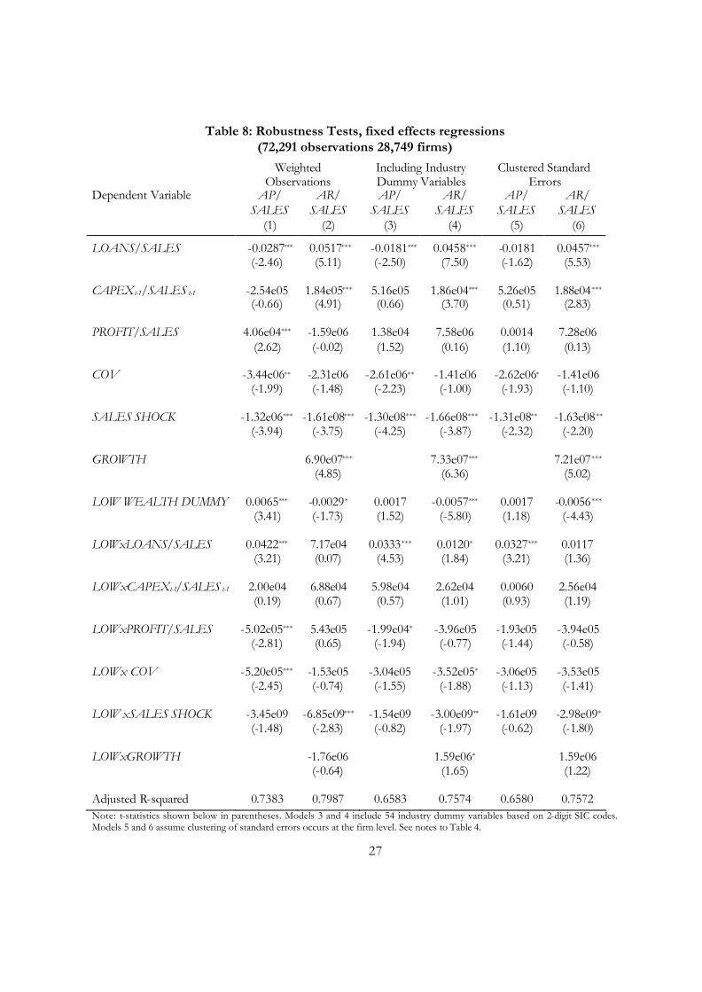
Table 8: Robustness Tests, fixed effects regressions (72,291 observations 28,749 firms)

Weighted Observations

Including Industry Dummy Variables

Clustered Standard Errors

Dependent Variable AP/ SALES

AR/ SALES

AP/ SALES

AR/ SALES

AP/ SALES

AR/ SALES

(1) (2) (3) (4) (5) (6)

LOANS/SALES -0.0287*** 0.0517*** -0.0181*** 0.0458*** -0.0181 0.0457*** (-2.46) (5.11) (-2.50) (7.50) (-1.62) (5.53) CAPEX t-1/SALES t-1 -2.54e05 1.84e05*** 5.16e05 1.86e04*** 5.26e05 1.88e04***

(-0.66) (4.91) (0.66) (3.70) (0.51) (2.83)

PROFIT/SALES 4.06e04*** -1.59e06 1.38e04 7.58e06 0.0014 7.28e06 (2.62) (-0.02) (1.52) (0.16) (1.10) (0.13) COV -3.44e06** -2.31e06 -2.61e06** -1.41e06 -2.62e06* -1.41e06 (-1.99) (-1.48) (-2.23) (-1.00) (-1.93) (-1.10) SALES SHOCK -1.32e06*** -1.61e08*** -1.30e08*** -1.66e08*** -1.31e08** -1.63e08** (-3.94) (-3.75) (-4.25) (-3.87) (-2.32) (-2.20) GROWTH 6.90e07*** 7.33e07*** 7.21e07*** (4.85) (6.36) (5.02) LOW WEALTH DUMMY 0.0065*** -0.0029* 0.0017 -0.0057*** 0.0017 -0.0056*** (3.41) (-1.73) (1.52) (-5.80) (1.18) (-4.43) LOWxLOANS/SALES 0.0422*** 7.17e04 0.0333*** 0.0120* 0.0327*** 0.0117 (3.21) (0.07) (4.53) (1.84) (3.21) (1.36) LOWxCAPEXt-1/SALES t-1 2.00e04 6.88e04 5.98e04 2.62e04 0.0060 2.56e04 (0.19) (0.67) (0.57) (1.01) (0.93) (1.19) LOWxPROFIT/SALES -5.02e05*** 5.43e05 -1.99e04* -3.96e05 -1.93e05 -3.94e05 (-2.81) (0.65) (-1.94) (-0.77) (-1.44) (-0.58) LOWx COV -5.20e05*** -1.53e05 -3.04e05 -3.52e05* -3.06e05 -3.53e05 (-2.45) (-0.74) (-1.55) (-1.88) (-1.13) (-1.41) LOW xSALES SHOCK -3.45e09 -6.85e09*** -1.54e09 -3.00e09** -1.61e09 -2.98e09* (-1.48) (-2.83) (-0.82) (-1.97) (-0.62) (-1.80) LOWxGROWTH -1.76e06 1.59e06* 1.59e06 (-0.64) (1.65) (1.22) Adjusted R-squared 0.7383 0.7987 0.6583 0.7574 0.6580 0.7572 Note: t-statistics shown below in parentheses. Models 3 and 4 include 54 industry dummy variables based on 2-digit SIC codes. Models 5 and 6 assume clustering of standard errors occurs at the firm level. See notes to Table 4.

28

To further test the robustness of the main findings, I also analyze several modified versions

of regression model 1 in Tables 4 and 5. Table 8 reports the results of estimating the main trade

credit usage and supply regressions with weighted observations, dummy variables for industry, and

controls for clustered standard errors. Weighted data can help adjust for the stratified sampling

methods used to collect some of the data. Industry-specific trade credit terms, and other industry-

specific factors may be better controlled for with the addition of industry dummy variables. Finally,

if the data are independent across firms but not necessarily independent over time within firms,

controlling for clustering in the data may be appropriate. This correction increases the standard

errors in the coefficient estimates and therefore reduces the t-statistics.

The results of these robustness tests are generally quite similar to the findings presented for

model 1 in Tables 4 and 5. Regressions with weighted observations have somewhat larger

coefficients for the bank credit variables in the AP/SALES regressions. Adding industry dummy

variables makes almost no difference to any of the coefficients. Correcting for clustered standard

errors reduces the precision of the coefficient estimates and weakens the findings somewhat.

Specifically LOANS/SALES in column (5) is no longer statistically significant, although the

coefficient on LOWxLOANS/SALES remains significant.

7. Conclusions

Burkart and Ellingsen (2004) model trade credit as means to help overcome a potential

moral hazard problem of borrowers diverting resources for private gain. This problem causes

credit rationing of both bank credit and trade credit, but because inputs are harder to divert than

cash and suppliers have a monitoring advantage for input use, suppliers can provide credit when

banks cannot. Their model explains why firms of different wealth categories face different degrees

of credit rationing and have different trade credit usage patterns. Aggregate investment is higher

29

when trade credit is available because it allows medium- and low-wealth firms to invest more than

their bank credit constraint would permit.

The findings here on trade credit usage provide considerable support for the theory’s main

predictions particularly with respect to medium-wealth firms. For the medium-wealth firms, bank

credit and trade credit usage is negatively related, consistent with trade credit playing the role of

less desirable substitute form of credit when bank credit is exhausted. These firms can increase

their reliance on trade credit if bank credit becomes less available. The firms identified as low-

wealth have a positive, complementary relationship between their bank credit and trade credit use,

suggesting they are constrained in both trade credit and bank credit markets. The findings on trade

credit usage seem robust to a large range of possible wealth thresholds. Nevertheless, the effects

for the low- and medium-wealth firms seem economically small despite being statistical significant.

The findings also suggest that there are very few high-wealth, unconstrained firms in

Canada. This is consistent with Nilsen (2002) who finds that all but the largest, bond-rated firms

appear to be finance-constrained. The data do not seem to support the view that firms supply less

trade credit when their investment opportunities increase insofar as sales growth captures

investment opportunities. I find that faster sales growth corresponds to provision of more trade

credit. Consistent with empirical evidence in Petersen and Rajan (1997), I also find that low-wealth,

declining and distressed firms provide proportionally more trade credit than more wealthy firms

do. These results and recent empirical research by Burkart et al (2005) on trade credit terms seem

to support Wilner’s (2000) bargaining power hypothesis. Further empirical work to discover why

distressed firms supply more trade credit than others and the cyclical implications of this behaviour

would also be of interest.

30

References:

Biais, Bruno and Christian Gollier. (1997). “Trade Credit and Credit Rationing,” The Review of Financial Studies , 10(4), 903—937. Burkart, Mike and Tore Ellingsen and Mariassunta Giannetti. (2005). “What You Sell is What You Lend? Explaining Tra de Credit Contracts,” Stockholm School of Economics. Working Paper. Burkart, Mike and Tore Ellingsen (2004). “In-Kind Finance: A Theory of Trade Credit,” American Economic Review, 94(3). 569—90. Demirguc-Kunt, Asli and Vojislav Makismovic. (2001). “Firms as Financial Intermediaries: Evidence from Trade Credit Data,” Working Paper , March 2001. Dun and Bradstreet. (1970). Handbook of Credit Terms. (New York: Dun and Bradstreet). Emery, Gary W. (1984). “A Pure Financial Explanation for Trade Credit,” Journal of Financial and Quantitative Analysis, 19(3), 271—285. Ferris, J. Stephen. (1981). “A Transactions Cost Theory of Trade Credit Use,” Quarterly Journal of Economics , 96(2), 243—70. Hansen, Bruce E. (2000) “Sample Splitting and Threshold Estimation,” Econometrica, 68(3) 575—603. Hubbard, Glen. (1998) “Capital Market Imperfections and Investment,” Journal of Economic Literature , 36(1) 193—225. Jain, Neelam. (2001). “Monitoring Costs and Trade Credit,” Quarterly Review of Economics and Finance, 41(2001), 89—110. Long, Michael S., Ileen B. Malitz, and S. Abraham Ravid. (1993). “Trade Credit, Quality Guarantees, and Product Marketability,” Financial Management, 22, 117—127. Mian, S. and C.W. Smith. (1992). “Accounts Receivables Management Policy: Theory and Evidence,” Journal of Finance , 47, 169—200. Nadiri, M. I. (1969). “The Determinants of Trade Credit in the U.S. Total Manufacturing Sector,” Econometrica, 47(1), 408—423. Ng, Chee K., Janet Kiholm Smith and Richard Smith. (1999). “Evidence on the Determinants of Credit Terms Used in Interfirm Trade,” Journal of Finance, 54(3), 1109—1129. Nilsen, Jeffrey (2002). “Trade Credit and the Bank Lending Channel,” Journal of Money, Credit and Banking, 34(1), 227—253.

31

Petersen, Mitchell A. and Raghuram G. Rajan (1997). “Trade Credit: Theories and Evidence,” Review of Financial Studies 10(3), 661—691. Smith, Janet Kiholm. (1987). “Trade Credit and Informational Asymmetry,” Journal of Finance, 42(4), 863—872. Wilner, Benjamin. (2000). “The Exploitation of Relationships in Financial Distress: The Case of Trade Credit,” Journal of Finance, 55(1), 153—178.

32

Appendix A: Overview of Burkart and Ellingsen Model

A risk-neutral entrepreneur with wealth ? = 0 has an opportunity to undertake an

investment. The investment which converts an input into output according to a production

function Q(I), where I is the input quantity actually invested into the project, and q is the total

quantity of inputs purchased. The input price is normalized to 1 and output price is p. The

entrepreneur is a price-taker in both the input and output markets. In a perfect credit market with

interest rate rBC , the entrepreneur would choose the first best level of investment I*(rBC) that solves

the first order condition, pQ’(I*) = 1+rBC. The entrepreneur’s wealth cannot fully fund this

investment level, ? < I*(rBC), so he must borrow. There are two possible sources of external

funding, bank credit and trade credit from the input supplier.

Banks and suppliers are assumed to operate in competitive markets, and they

simulanteously offer a loan contract to the entrepreneur. Since the entrepreneur may divert some

project resources for private gain rather than investment, there is a moral hazard problem for both

types of creditors and they ration the credit available to him. The bank loan offer specifies the

bank credit limit BC and interest rate rBC . Similarly, the supplier’s loan contract indicates the

maximum trade credit it will provide TC , input purchases q, and trade credit interest rate rTC .

A key assumption of the BE model is that banks and suppliers differ in their exposure to

moral hazard because suppliers have a monitoring advantage over the banks. Suppliers observe

input purchases and revenues but not investment, whereas banks observe only revenues. The

supplier conditions its lending on input purchases, ( )TC q , where bank credit limit is just a fixed

amount, BC .

33

If the entrepreneur diverts a unit of cash, he gets some private benefit f < 1, (so f can be

viewed as creditor vulnerability). Since inputs have to be converted to cash and then diverted, the

private gain is from diverting a unit of input is ßf is less the private gain from diverting cash, f ,

and it depends on how liquid the input is, ß =1. More liquid inputs have larger ß and are more

attractive for diversion.

Since banks are assumed to be competitive, they earn zero profits and equilibrium bank

interest rates normalized at rBC = 0. The trade credit interest rate rTC is assumed to be higher than

rBC, so the entrepreneur uses trade credit only if the cash available from his own wealth and bank

credit are less than the desired investment level, i.e. if *( )TCBC I rω + < . If the entrepreneur does

not divert any resourc es, he buys inputs q BC TCω= + + and his trade credit utilized is TCU, just

enough to invest the desired amount or up to the trade credit limit,

(1) { }*min ( ) , ( )UTCTC I r BC TC qω= − −

After accepting credit offers from a bank and a supplier, the entrepreneur chooses q, I, BC,

and TC to maximize his utility,

(2) { } [ ]max 0, ( ) (1 ) ( ) ( )TCU pQ I BC r TC q I BC TC qϕ β ω= − − + + − + + + −

subject to the constraints,

( )

q B C T CI q

BC B C

TC TC q

ω≤ + +≤

≤

≤

The first term in the utility function is the entrepreneur’s residual return from investing the

available resources, and the second term is his private benefit from diverting inputs and cash

respectively. In addition to four constraints shown in (2), BE derive two incentive compatibility

34

constraints shown in equations (3) and (4), to ensure that investment generates a residual return to

the entrepreneur that is greater than or equal to his private payoff from diversion. Equation (3)

ensures the entrepreneur does not exhaust all available trade credit and then divert all inputs and

remaining cash. Equation (4) is required to prevent the entrepreneur from not purchasing any

inputs at all and just diverting all the cash.

(3) ( ) (1 ) ( )U UTCpQ BC TC BC r TC BC TCω ϕβ ω+ + − − + ≥ + +

(4) ( ) (1 ) ( )U UTCpQ BC TC BC r TC BCω ϕ ω+ + − − + ≥ +

Constraints (3) and (4) give the equilibrium credit limits BC and TC . Based on their differing

credit limits, entrepreneurs with different wealth levels have different credit usage and investment

behaviour, as summarized in Table 1 in the text (based on BE’s Proposition 2). BE analyze the

comparative statics of the TC and BC limits with respect to changes in output prices, wealth,

creditor vulnerability, input liquidity and trade credit interest rates which form the basis for the

regression coefficient tests. These are summarized in Table 2 in the text (from BE’s Propositions 3

and 4.)

35

Appendix B: Variable Definitions and Data Description

Variable Description

Accounts Payable (AP)

Accounts Payable from Trade (arising from sale of goods and services) measured in 1997 Canadian dollars. Nominal values converted to real using the GDP deflator.

Accounts Receivable (AR)

Accounts Receivable from Trade (arising from purchase of goods and services), measured in 1997 Canadian dollars.

Net Trade Credit AR – AP

Shareholder Equity Assets - Liabilities

Sales Sales of goods and services in 1997 dollars.

Profit Net Income after all items have been included (taxes, income from affiliates, extraordinary items etc.), measured in 1997 dollars.

Loans Loans from Non-Affiliates in 1997 dollars.

Capital Expenditure

Net Capital Expenditures, measured in 1997 dollars.

Coverage Ratio (COVRATIO)

Earnings Before Interest and Taxes (EBIT) / Interest Expense on Debt, where EBIT is calculated as Net Profit Before Tax + Interest Expense on Debt

Growth Percentage change in sales from previous year.

The data come from Statistics Canada’s unpublished microdata files of the Financial and

Taxation Statistics for Enterprises (FTSE) annual database, which is a detailed database of balance

sheet, income statement and corporate income tax data. The dataset contains enterprise-level data

that are collected using a combination of survey data and administrative data from corporate tax

returns provided by Canada Customs and Revenue Agency (CCRA). The sample is stratified three

ways: by industry, by country of control, and by size. Industries are defined using 63 groupings of

the 1980 2-digit SICs. Within each industry, there are three strata for country of control: Canada,

the United States or other. Finally, within the country of control stratum, there are multiple size

categories based on the firm’s assets or revenues. The largest firms in each industry are sampled

with certainty, although the size bounds vary by industry. For most industries this “take-all”

36

stratum consists of the largest firms with assets or annual revenues of more than $25 million in

current dollars. The second strata consists of smaller firms that are randomly selected for inclusion

in the survey. In the take-some stratum, data were collected through a mix of surveys and

administrative tax files. The final stratum of the sample consists of the smallest firms which were

not surveyed, so all their data come from the tax return files.

I select only the non-financial firms from the dataset, and also remove observations from

the sample if regression variables seem to have very extreme values. Specifically I restrict the

sample to those observations where the dependent variables in the regressions, the accounts

payable to sales and accounts receivable to sales ratios, were between zero and one; this removes

approximately 1% of the original observations. Observations where sales are negative are also

omitted, as are the cases where ratios of capital expenditures to sales or bank loans to sales were

zero or greater than the 95th percentile value.