TRACING ABUNDANCES IN GALAXIES WITH THE SPITZER SPACE

TELESCOPE INFRARED SPECTROGRAPH

A Dissertation

Presented to the Faculty of the Graduate School

of Cornell University

in Partial Fulfillment of the Requirements for the Degree of

Doctor of Philosophy

by

Shannon Laura Gutenkunst

May 2008

c© 2008 Shannon Laura Gutenkunst

ALL RIGHTS RESERVED

TRACING ABUNDANCES IN GALAXIES WITH THE SPITZER SPACE

TELESCOPE INFRARED SPECTROGRAPH

Shannon Laura Gutenkunst, Ph.D.

Cornell University 2008

As a galaxy evolves, its stars change the amounts (abundances) of elements within

it. Thus determining the abundances of these elements in different locations within

a galaxy traces its evolution. This dissertation presents abundances of planetary

nebulae in our Galaxy and of H II regions in a nearby galaxy (M51). Observations

at optical wavelengths dominated such studies in the past. However, abundances

determined from infrared lines have the advantages that they are less affected by

extinction and the adopted electron temperature. We employ spectra from the

Spitzer Space Telescope Infrared Spectrograph and derive abundances for argon,

neon, sulfur, and oxygen. These elements are not usually affected by nucleosyn-

thesis in the progenitor stars of planetary nebulae, and thus their abundances

trace the amounts of these elements in the progenitor cloud. The abundances of

these elements in H II regions trace the amounts of these elements in the interstellar

medium today. We do a case study of abundances in the planetary nebula IC 2448,

finding that it has subsolar abundances, which indicates that the progenitor star

formed out of subsolar material. We also derive abundances and assess the dust

properties of eleven planetary nebulae in the Bulge of the Milky Way. We find that

the abundances from these planetary nebulae do not follow the abundance trend

observed in planetary nebulae in the Disk. This points toward separate evolution

for the Bulge and Disk components. Additionally, we find peculiar dust proper-

ties in planetary nebulae in the Bulge which indicate that the progenitors of these

nebulae evolved in binaries. Finally, we make a pilot study of the abundances in

H II regions across the galaxy M51.

BIOGRAPHICAL SKETCH

Shannon was born on May 23, 1979 in Albuquerque, New Mexico to Norman

and Sharon Guiles. They all moved to Redlands, California when Shannon was six

months old. Her brother, Jason, was born there on February 3, 1981, and Shannon

cannot remember life without him. As Shannon grew up, her father helped her

when she got stuck on math or science homework and her mother taught her how

to learn from books. She also learned a lot from tutoring her brother in math when

he wanted help.

Shannon graduated from Redlands High School in 1997. She went on to attend

the University of California, San Diego (UCSD) where she received her Bachelor’s

Degree in Physics in 2001. During her undergraduate years she participated in

three Research Experience for Undergraduates (REU) programs: (1) with Prof.

Ami Berkowitz at UCSD on magnetic materials, (2) in Prof. Michael Wiescher’s

group at the University of Notre Dame in nuclear physics, and (3) with Prof.

George Fuller at UCSD in theoretical astrophysics. The most enjoyable of these

REU programs was working with George Fuller, who encouraged her in applying

to graduate schools, and for part of the year after she graduated she continued to

work with him and his graduate student Jason Pruet.

In August of 2002, Shannon and her mom took a road trip to Ithaca, New

York where Shannon became a graduate student in the Department of Physics

at Cornell University. During her first summer in graduate school she worked in

biophysics with Prof. Carl Frank, but ultimately decided that biophysics was not

for her. After her second year in graduate school she joined Prof. Jim Houck’s

group in Astronomy, and she has worked in this group for the last four years, with

her work in this group culminating in her dissertation. She also met her husband,

Ryan Gutenkunst, while at Cornell, and they married on April 29, 2007.

iii

To my husband Ryan, my parents Sharon and Norman Guiles, my brother Jason

Guiles, and my grandma Frieda Maloney.

iv

ACKNOWLEDGEMENTS

First and foremost, I thank Jeronimo Bernard-Salas, who mentored me during my

last two years of research. The work I have done with him forms the bulk of this

dissertation. I am grateful to him for paying attention when I needed help, for

sharing and explaining his code for calculating abundances, and for finding my

mistakes and pointing me in the right direction to fix them (although of course

any mistakes left in this dissertation are my fault and not his). Thanks also to Jim

Houck for providing me with such a great opportunity to work on data from the

Spitzer Space Telescope Infrared Spectrograph. I feel fortunate that I happened to

be a graduate student when and where I had the chance to work with data from

such an important instrument. Additionally, thanks to all of the other members

of my special committee: Terry Herter, Saul Teukolsky, and Ira Wasserman.

I thank the past and present members of the Spitzer IRS group at Cornell whom

I have had the pleasure to work with (in alphabetical order): Don Barry, Jeronimo

Bernard-Salas, Bernhard Brandl, Vassilis Charmandaris, Daniel Devost, Duncan

Farrah, Elise Furlan, Peter Hall, Lei Hao, Terry Herter, James Higdon, Sarah

Higdon, Jim Houck, Jason Marshall, Laurie McCall, Greg Sloan, Henrik Spoon,

Keven Uchida, Dan Weedman, and Yanling Wu. All of them have helped me at

some point, and their support has meant a lot to me. I would like to single out

Don Barry who kept my computer running happily, Elise Furlan for teaching me

the intricacies of SMART, Peter Hall for keeping SMART running, Laurie McCall

for keeping things in the group running smoothly, Greg Sloan for answering my

questions about dust, and Yanling Wu for being a kind and supportive office mate

who never hesitated to answer my questions.

Thanks to all of my co-authors on the two papers about planetary nebulae.

Jeronimo Bernard-Salas and Stuart Pottasch gave me thorough comments and

v

suggestions on the two papers, which indubitably made the papers fly through

the review process with ease; their expertise in the subject helped immensely.

Jeronimo also planned the observations on which the second paper was based.

Also thanks to my other co-authors on those papers: Tom Roellig (who planned

the observations on which the first paper was based), Greg Sloan (who helped with

the interpretation of the dust features in the second paper), and Jim Houck (who

gave me helpful comments on both papers and donated the IRS GTO time for the

observations for the second paper).

I also thank Daniel Devost and Terry Herter for helping me with a project to

take data at Palomar, and to Thomas Jarrett for showing me how to best use the

WIRC instrument there for narrow-band imaging and setting me up to use his

data reduction software. Thanks to James Lloyd and Don Banfield for letting me

use some of their telescope time to learn how to use the WIRC instrument before

my observing run. Thanks also to the night assistant there, Jean Mueller.

Also thanks to NASA for funding my research. This work is based in part on

observations made with the Spitzer Space Telescope, which is operated by the Jet

Propulsion Laboratory, California Institute of Technology under NASA contract

1407. Support for this work was provided by NASA through Contract Number

1257184 issued by JPL/Caltech.

Additionally, I thank the members of the Ithaca Area Toastmasters Club. Their

support and positive feedback have helped me improve my public speaking skills,

which in turn helped me when I gave presentations on my work and talks for out-

reach. I also found their friendship, cheer, and different outlook on life invaluable.

Finally, I thank my family. My parents and grandparents always encouraged

me to do my best, and without that encouragement I would not be here. My

brother is one of my best friends, and I appreciate his support. Most of all, I

vi

thank my husband Ryan. The rest of my family lives across the country. Ryan’s

presence here and his love, support, and encouragement helped buoy me through

the deep and sometimes turbulent waters of graduate school.

vii

TABLE OF CONTENTS

Biographical Sketch . . . . . . . . . . . . . . . . . . . . . . . . . . . . . . iiiDedication . . . . . . . . . . . . . . . . . . . . . . . . . . . . . . . . . . . ivAcknowledgements . . . . . . . . . . . . . . . . . . . . . . . . . . . . . . vTable of Contents . . . . . . . . . . . . . . . . . . . . . . . . . . . . . . . viiiList of Tables . . . . . . . . . . . . . . . . . . . . . . . . . . . . . . . . . xList of Figures . . . . . . . . . . . . . . . . . . . . . . . . . . . . . . . . . xi

1 Introduction 11.1 Elements and the Evolution of the Galaxy . . . . . . . . . . . . . . 2

1.1.1 Creation of the Elements . . . . . . . . . . . . . . . . . . . . 21.1.2 Formation and Evolution of the Galaxy . . . . . . . . . . . . 4

1.2 Photoionization Regions . . . . . . . . . . . . . . . . . . . . . . . . 71.2.1 Planetary Nebulae . . . . . . . . . . . . . . . . . . . . . . . 101.2.2 H II Regions . . . . . . . . . . . . . . . . . . . . . . . . . . . 12

1.3 What We Can Learn from Spectra of Photoionization Regions . . . 131.3.1 Extinction . . . . . . . . . . . . . . . . . . . . . . . . . . . . 131.3.2 Electron Density and Temperature . . . . . . . . . . . . . . 141.3.3 Abundances . . . . . . . . . . . . . . . . . . . . . . . . . . . 151.3.4 Ionizing Radiation Field . . . . . . . . . . . . . . . . . . . . 20

1.4 Dust: Gemstones and Carcinogens in Space . . . . . . . . . . . . . 211.4.1 Silicates . . . . . . . . . . . . . . . . . . . . . . . . . . . . . 231.4.2 Polycyclic Aromatic Hydrocarbons (PAHs) . . . . . . . . . . 25

1.5 Observing with the Spitzer Space Telescope . . . . . . . . . . . . . 261.6 In This Dissertation . . . . . . . . . . . . . . . . . . . . . . . . . . . 29

2 The Spitzer IRS Infrared Spectrum and Abundances of the Plan-etary Nebula IC 2448 302.1 Abstract . . . . . . . . . . . . . . . . . . . . . . . . . . . . . . . . . 302.2 Introduction . . . . . . . . . . . . . . . . . . . . . . . . . . . . . . . 302.3 Spitzer Observations and Data Reduction . . . . . . . . . . . . . . . 322.4 Optical and UV Data . . . . . . . . . . . . . . . . . . . . . . . . . . 382.5 Data Analysis . . . . . . . . . . . . . . . . . . . . . . . . . . . . . . 40

2.5.1 Extinction Correction . . . . . . . . . . . . . . . . . . . . . . 402.5.2 Electron Density . . . . . . . . . . . . . . . . . . . . . . . . 422.5.3 Electron Temperature . . . . . . . . . . . . . . . . . . . . . 432.5.4 Abundances . . . . . . . . . . . . . . . . . . . . . . . . . . . 43

2.6 Discussion . . . . . . . . . . . . . . . . . . . . . . . . . . . . . . . . 472.7 Conclusions . . . . . . . . . . . . . . . . . . . . . . . . . . . . . . . 50

viii

3 Chemical Abundances and Dust in Planetary Nebulae in theGalactic Bulge 523.1 Abstract . . . . . . . . . . . . . . . . . . . . . . . . . . . . . . . . . 523.2 Introduction . . . . . . . . . . . . . . . . . . . . . . . . . . . . . . . 533.3 Spitzer IRS Data . . . . . . . . . . . . . . . . . . . . . . . . . . . . 55

3.3.1 Observations . . . . . . . . . . . . . . . . . . . . . . . . . . 553.3.2 Source Selection . . . . . . . . . . . . . . . . . . . . . . . . . 553.3.3 Data Reduction . . . . . . . . . . . . . . . . . . . . . . . . . 59

3.4 Supplementary Data . . . . . . . . . . . . . . . . . . . . . . . . . . 603.5 Data Analysis . . . . . . . . . . . . . . . . . . . . . . . . . . . . . . 66

3.5.1 Abundances . . . . . . . . . . . . . . . . . . . . . . . . . . . 663.5.2 Crystalline Silicates . . . . . . . . . . . . . . . . . . . . . . . 763.5.3 PAHs . . . . . . . . . . . . . . . . . . . . . . . . . . . . . . 76

3.6 Discussion . . . . . . . . . . . . . . . . . . . . . . . . . . . . . . . . 773.6.1 Elemental Abundances . . . . . . . . . . . . . . . . . . . . . 773.6.2 Crystalline Silicates . . . . . . . . . . . . . . . . . . . . . . . 903.6.3 PAHs . . . . . . . . . . . . . . . . . . . . . . . . . . . . . . 923.6.4 Dual Chemistry Nebulae . . . . . . . . . . . . . . . . . . . . 93

3.7 Conclusions . . . . . . . . . . . . . . . . . . . . . . . . . . . . . . . 94

4 Abundances in H II Regions Across M51 from Spitzer Spectra 964.1 Introduction . . . . . . . . . . . . . . . . . . . . . . . . . . . . . . . 964.2 Observations and Data Reduction . . . . . . . . . . . . . . . . . . . 98

4.2.1 Spitzer Data . . . . . . . . . . . . . . . . . . . . . . . . . . . 984.2.2 Hα Map . . . . . . . . . . . . . . . . . . . . . . . . . . . . . 103

4.3 Data Analysis . . . . . . . . . . . . . . . . . . . . . . . . . . . . . . 1054.3.1 Extinction Correction . . . . . . . . . . . . . . . . . . . . . . 1054.3.2 Electron Temperature and Density . . . . . . . . . . . . . . 1054.3.3 Abundances . . . . . . . . . . . . . . . . . . . . . . . . . . . 106

4.4 Discussion . . . . . . . . . . . . . . . . . . . . . . . . . . . . . . . . 1084.4.1 Ionizing Radiation Field . . . . . . . . . . . . . . . . . . . . 1084.4.2 Neon to Sulfur Abundance Ratio . . . . . . . . . . . . . . . 109

4.5 Conclusions . . . . . . . . . . . . . . . . . . . . . . . . . . . . . . . 110

ix

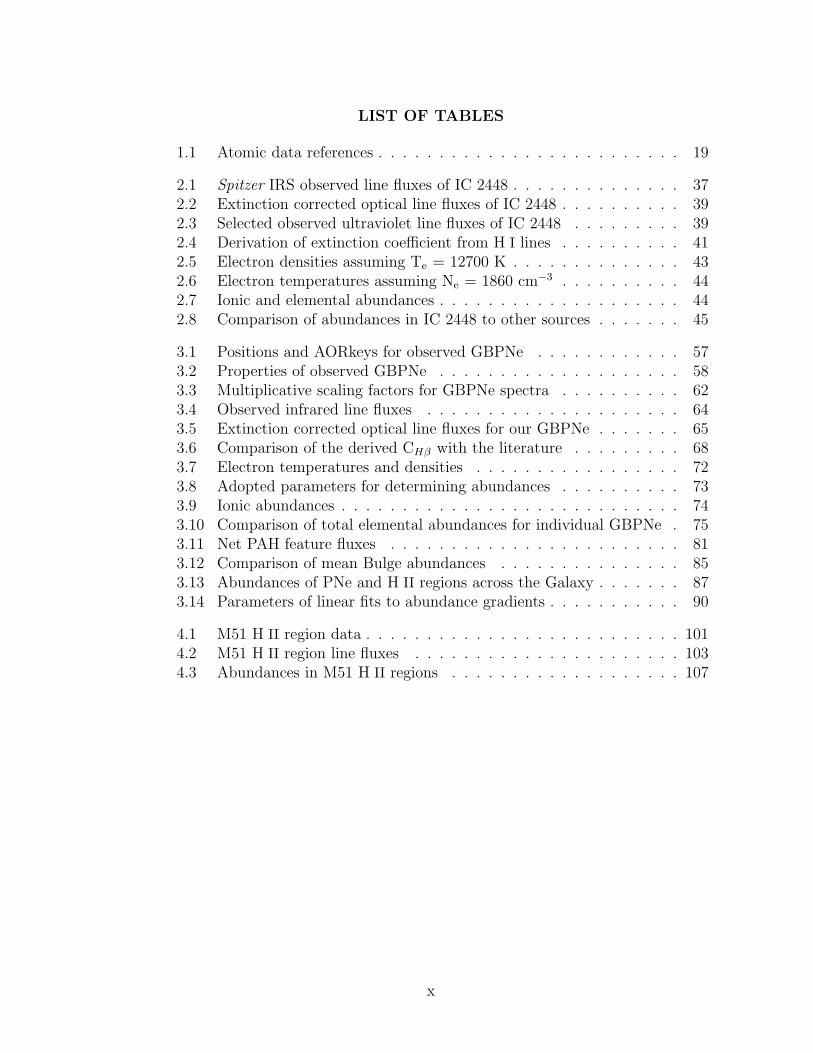
LIST OF TABLES

1.1 Atomic data references . . . . . . . . . . . . . . . . . . . . . . . . . 19

2.1 Spitzer IRS observed line fluxes of IC 2448 . . . . . . . . . . . . . . 372.2 Extinction corrected optical line fluxes of IC 2448 . . . . . . . . . . 392.3 Selected observed ultraviolet line fluxes of IC 2448 . . . . . . . . . 392.4 Derivation of extinction coefficient from H I lines . . . . . . . . . . 412.5 Electron densities assuming Te = 12700 K . . . . . . . . . . . . . . 432.6 Electron temperatures assuming Ne = 1860 cm−3 . . . . . . . . . . 442.7 Ionic and elemental abundances . . . . . . . . . . . . . . . . . . . . 442.8 Comparison of abundances in IC 2448 to other sources . . . . . . . 45

3.1 Positions and AORkeys for observed GBPNe . . . . . . . . . . . . 573.2 Properties of observed GBPNe . . . . . . . . . . . . . . . . . . . . 583.3 Multiplicative scaling factors for GBPNe spectra . . . . . . . . . . 623.4 Observed infrared line fluxes . . . . . . . . . . . . . . . . . . . . . 643.5 Extinction corrected optical line fluxes for our GBPNe . . . . . . . 653.6 Comparison of the derived CHβ with the literature . . . . . . . . . 683.7 Electron temperatures and densities . . . . . . . . . . . . . . . . . 723.8 Adopted parameters for determining abundances . . . . . . . . . . 733.9 Ionic abundances . . . . . . . . . . . . . . . . . . . . . . . . . . . . 743.10 Comparison of total elemental abundances for individual GBPNe . 753.11 Net PAH feature fluxes . . . . . . . . . . . . . . . . . . . . . . . . 813.12 Comparison of mean Bulge abundances . . . . . . . . . . . . . . . 853.13 Abundances of PNe and H II regions across the Galaxy . . . . . . . 873.14 Parameters of linear fits to abundance gradients . . . . . . . . . . . 90

4.1 M51 H II region data . . . . . . . . . . . . . . . . . . . . . . . . . . 1014.2 M51 H II region line fluxes . . . . . . . . . . . . . . . . . . . . . . 1034.3 Abundances in M51 H II regions . . . . . . . . . . . . . . . . . . . 107

x

LIST OF FIGURES

1.1 Diagram of the structure of the Milky Way . . . . . . . . . . . . . 51.2 Example IRS spectrum . . . . . . . . . . . . . . . . . . . . . . . . 91.3 Configuration as well as Ne and Te diagnostics for S III . . . . . . . 161.4 Synthetic spectra of the radiation from an instantaneous starburst 221.5 Example of crystalline silicate features in an IRS spectrum . . . . . 241.6 Image of an olivine grain . . . . . . . . . . . . . . . . . . . . . . . 241.7 Structure of forsterite . . . . . . . . . . . . . . . . . . . . . . . . . 251.8 Example structures of PAH molecules . . . . . . . . . . . . . . . . 261.9 Example of PAH features in an IRS spectrum . . . . . . . . . . . . 27

2.1 The Spitzer IRS spectrum of IC 2448. . . . . . . . . . . . . . . . . 352.2 Close-ups of emission lines in the Spitzer spectrum of IC 2448 . . . 36

3.1 Spitzer IRS spectra of our GBPNe . . . . . . . . . . . . . . . . . . 633.2 Continuum subtracted spectra showing crystalline silicates . . . . . 803.3 Profiles of PAH features . . . . . . . . . . . . . . . . . . . . . . . . 823.4 Abundances of Bulge and Disk PNe versus galactocentric distance . 893.5 Comparison of mean 28 and 33 µm silicate features . . . . . . . . . 91

4.1 SINGS Hα continuum subtracted image of M51 . . . . . . . . . . . 994.2 IRS spectra of H II regions in M51 . . . . . . . . . . . . . . . . . . 1024.3 M51 H II region Ne III/Ne II flux ratio versus distance . . . . . . . 1084.4 M51 (Ne++Ne++)/(S+++S3+) abundance ratio versus distance . . 109

xi

CHAPTER 1

INTRODUCTION

On Earth, some snakes in the pit viper family have sacks on the sides of their

heads that allow them to detect infrared light, or heat. This ability to “see” in

the infrared allows the snakes to detect delectable rodents in dark underground

tunnels where there is no optical light. Just as viewing objects on Earth in the

infrared can uncover secrets hidden from optical light, viewing objects in space in

the infrared allows astronomers to probe precious pieces of the cosmos unseen in

the optical. For example, dust hinders optical studies because it absorbs optical

light, but this same dust re-radiates the light in the infrared. Astronomers can

identify the type of dust by looking at the features they produce in the infrared

spectra (see §1.4).

Infrared spectra also allow astronomers to determine the amounts of various

elements (abundances) by measuring fluxes in infrared emission lines. Abundances

from different locations in a galaxy give information about its formation and evo-

lution. In the past, observations at optical wavelengths dominated abundance

studies. However, studies at other wavelengths give new insights. This disserta-

tion concentrates on what we can learn from infrared spectra of photoionization

regions (specifically planetary nebulae and H II regions) in our Galaxy and M51

(NGC 5194). First we derive abundances of the planetary nebula IC 2448 in the

Disk of the Milky Way, finding that it has abundances of argon, neon, sulfur, and

oxygen slightly lower than solar which implies that the cloud from which the pro-

genitor star formed had a subsolar abundance. Then we derive abundances for

eleven planetary nebulae in the Galactic Bulge, finding that these nebulae do not

follow the trend of abundance versus galactocentric distance displayed by nebulae

in the Disk, thus indicating the separate evolution of the Bulge and the Disk. Ad-

1

ditionally we find that these nebulae in the Bulge have different dust properties

than typical for nebulae in the Disk, and the dust signatures indicate that the

progenitors of many of the Bulge nebulae probably evolved in binary systems. Fi-

nally we derive abundances from H II regions across M51; while we cannot derive

accurate abundances with respect to hydrogen, we can make an approximation of

the neon to sulfur abundance ratio which appears to show that Ne/S decreases

with increasing distance from the center, but this probably is not a real affect.

The next section (§1.1) discusses the formation of elements and how determin-

ing elemental abundances in different parts of a galaxy gives clues about how it

formed and evolved. §1.2 summarizes the important properties of photoionization

regions that are relevant to this work. Then §1.3 discusses what we can learn from

spectra of these photoionization regions. §1.4 discusses the types of dust which

produce features in infrared spectra of planetary nebulae and H II regions. §1.5

gives information about the Spitzer Space Telescope Infrared Spectrograph (IRS)

which made the bulk of the observations for this dissertation. Finally §1.6 gives a

brief description of the remaining chapters of the dissertation.

1.1 Elements and the Evolution of the Galaxy

1.1.1 Creation of the Elements

Big Bang nucleosynthesis created the elements of hydrogen, helium, lithium, and

trace amounts of beryllium. Stars create the rest. Understanding what types of

stars make which elements and on what timescales these elements form is vital for

understanding how galaxies form and evolve. A summary of when various elements

are made in different types of stars follows; for more details see Matteucci (2001)

on which this discussion is based.

Massive stars with masses above ∼8 M¯ end their lives in core collapse (Type

2

II and Ib/c) supernovae (SNe) explosions. They produce the bulk of the oxygen,

the principal element in the global abundance, as well as the bulk of other α-

elements (such as argon, neon, and sulfur) which are formed by fusing together

α particles (helium-4 nuclei, He+2) either in the core of the star or during the

explosion (Matteucci, 2008). These supernova also produce other heavy elements

through the r-process, the rapid capture of neutrons onto seed nuclei relative to

the timescale of β decay (Woosley et al., 1994). Such massive stars have short

lifetimes in the range of 1 to 10 Myr.

Type Ia SNe caused by exploding white dwarfs in binary systems produce

most (∼70%) of the iron and small amounts of other heavy elements (Matteucci &

Greggio, 1986). Because the progenitors of these Type Ia SNe are low-intermediate

mass stars, they have long lifetimes of several 10 Myr to over 10 Gyr. These low

mass stars live longer than the massive stars which produce oxygen and other α-

elements, and thus there is a delay between the iron and α-element enrichment of

the ISM for a group of stars which formed at the same time. Thus the abundance

ratio of α-elements to iron [α/Fe] can serve as a ‘cosmic clock’.

Low and intermediate mass stars with masses in the range ∼0.8 to ∼8 M¯

ignite helium in their core and dredge-up episodes occur which bring the processed

material from the core to the surface. The stars then eject some of their material in

stellar winds during the Red Giant Branch (RGB) and Asymptotic Giant Branch

(AGB) phases (Iben & Renzini, 1983). Radiation from the central star ionizes

this ejected material which then “lights up” during a planetary nebula (PN) phase

before the star ends its life as a carbon-oxygen white dwarf. In this way the

stars restore part of their processed and unprocessed material to the interstellar

medium, enriching the interstellar medium in helium, carbon, nitrogen, and the

heavy s-process elements which are made by the slow capture of neutrons onto

3

seed nuclei relative to the β decay timescale (Iben & Renzini, 1983). While each

of these stars has much less mass and evolves more slowly than a massive star,

the Galaxy contains many more of these low-intermediate mass stars, and they

probably produce most of the nitrogen and carbon in the interstellar medium

today (Chiappini et al., 2003), making carbon mainly as a primary element and

making nitrogen mainly as a secondary element during hydrogen burning (in the

CNO cycle).

In summary, stars with masses (∼8 M¯–100 M¯) which explode as core collapse

SNe make most of the α-elements (like oxygen, neon, sulfur, and argon) as well as

heavy r-process elements on short timescales (1–10 Myr). Low–intermediate mass

stars that end their lives as Type Ia SNe produce most of the iron and limited

amounts of other heavy elements on long timescales (10 Myr to 10+ Gyr). The

other low–intermediate mass stars produce helium, carbon, nitrogen and heavy

s-process elements, releasing their material into the interstellar medium also on

long timescales. The abundance ratio of an element released in to the interstellar

medium on a short timescale to that of an element released on a long timescale

serves as a cosmic clock, revealing the nature of the chemical evolution of a galaxy.

1.1.2 Formation and Evolution of the Galaxy

Figure 1.1 shows a diagram of the different parts of the Milky Way. The Disk

(including the Thin and Thick Disks) contains gas and stars. The Thin Disk

contains most of the mass of the Disk and the young stars; the Thick Disk contains

only a few percent of the total mass of the Disk and most of the old stars. The Bulge

resides at the center of the Disk, and a spherical Outer Halo of stars surrounds

the Disk and Bulge, with a spherical dark matter Halo extending out beyond the

stellar Halo (Carroll & Ostlie, 1996). The Inner Halo of stars has a more squashed

4

Sun

8 kpc

2 kpc

15 kpc

25 kpc

50 + kpc

Thin Disk

Thick Disk

BulgeGalactic Center

Inner Halo

Outer Halo

Figure 1.1 Diagram of the structure of the Milky Way; not to scale. Figure designafter Matteucci (2001) Figure 1.1; distances in the figure taken from Carroll &Ostlie (1996), except for the boundary between the Inner and Outer Halo notgiven in Carroll & Ostlie (1996) which is from Carollo et al. (2007). The Outerstellar Halo extends out to a radius of about 50 kpc, but the dark matter Haloextends beyond a radius of 100 kpc.

5

shape (Carollo et al., 2007). These different parts of the Galaxy have different

chemical compositions which gives information about their evolution, as discussed

below.

Determining how the Galaxy formed and evolved from the abundances and

motions of stars began in the 1960’s with the paper by Eggen et al. (1962). They

found that high velocity stars with lower abundances move in more elliptical orbits

and have smaller angular momenta than stars with higher abundances, and they

concluded that the old low abundance stars populate a Halo formed out of a

quick infall of a cloud of gas. In the 1970’s Searle & Zinn (1978) questioned this

picture of Halo formation. They found that some globular clusters in the Halo

were much older than others, implying that the Halo could not have formed as

quickly as proposed by Eggen et al. (1962). They suggested that the Halo formed

out of many cloud fragments, which may themselves already have formed stars and

globular clusters.

Radial elemental abundance gradients indicate how the Disk formed. Different

elements can have different gradients because they are made in different processes

in stars. That is, the gradient of each element depends on the timescale for pro-

duction (and release into the interstellar medium) of that element. For example,

nitrogen and iron have slightly steeper gradients than oxygen because long-lived

low to intermediate mass stars produce most of the nitrogen (released during the

PN phase) and iron (from Type Ia SNe) whereas short-lived high mass stars pro-

duce most of the oxygen; additionally nitrogen is a secondary element and thus is

produced proportionally to the original oxygen abundance. Characterizing these

abundances gives important information on when star formation occurred in dif-

ferent regions of the Galaxy (Matteucci, 2001).

Several studies comparing galactic chemical evolution models of the Milky Way

6

with observationally derived abundances give the following description of its for-

mation and evolution, but this is still an area of active research. The Inner Halo

and Bulge form out of an infall episode on a short timescale of ∼1 Gyr (Buonanno

et al., 1994; Ballero et al., 2007). The Outer Halo forms with a longer timescale of

∼5 Gyr by accreting satellite stellar systems and/or extragalactic gas (Buonanno

et al., 1994; Carollo et al., 2007). The Thin Disk forms out of another infall episode

inside-out and more slowly — with the timescale increasing linearly with galac-

tocentric distance with a value of ∼7 Gyr in the solar neighborhood (Chiappini

et al., 1997). The inside-out Disk formation is brought about because the outer

parts of the Disk form later as gas with higher angular momentum settles into

the plane of the Disk at larger radii, and this theory can reproduce the observed

abundance gradients along the Disk (Matteucci, 2001). The Thick Disk may have

formed from mergers of satellite galaxies with the primordial Thin Disk (Quinn

et al., 1993). Other spiral galaxies may form through similar processes.

1.2 Photoionization Regions

Photoionization regions are present around newly formed stars (H II regions),

dying stars (planetary nebulae, PNe), and accreting black holes; the following

discussion on such regions is based on Ferland (2003) and Osterbrock (1989) where

the reader can find further details. Ultraviolet (and optical to a lesser extent)

photons emitted by a radiation source (such as a star) inside or nearby a gaseous

nebula heat its dust grains to ∼100 K which then re-radiate the energy in the

infrared, causing the continuum in infrared spectra. Additionally these photons

collide with atomic hydrogen (hydrogen being the most abundant element in the

Universe and in these nebulae) and photionize it. The photoelectrons ejected in

this process then (elastically) collide with each other and ions, reaching a Maxwell-

7

Boltzmann velocity distribution characterized by a unique electron temperature,

which is usually between 5000 and 20000 K. A typical photoelectron remains in the

continuum for several years, often (elastically) colliding with other photoelectrons,

and every few weeks or so it (inelastically) collides with an ion, losing part of its

kinetic energy to internal excitations in the ion.

At the low densities of these nebulae (Ne . 104 cm−3) collisional de-excitation

of these excited levels of ions does not occur often, and thus these excited levels

radiate photons to reach the ground state, causing forbidden lines in the spectra

of these nebulae. The lines are called ‘forbidden’ because the energy transitions

which produce them (electric quadrupole or magnetic dipole) are less likely to

occur than the ‘permitted’ (electric dipole) transitions; additionally the forbidden

lines cannot be seen in laboratory experiments on Earth because even in the best

man-made vacuum the density is high enough for collisional de-excitation to occur.

The permitted transitions do not dominate the spectra of photoionization regions

because they often require a very high energy to excite (and would only occur

in the far-UV), and thus it is important to study the forbidden transitions in

photoionization regions.

Measuring the fluxes of these forbidden lines along with other information al-

lows us to determine elemental abundances in these regions, as discussed more in

§1.3.3. The brightest forbidden lines are labeled in the the Spitzer IRS spectrum of

the Bulge planetary nebulae PNG000.7+04.7 shown in Figure 1.2. The forbidden

lines are denoted by square brackets surrounding an abbreviation of the element

and a roman numeral equal to the ionization state plus one, e.g. a forbidden line

of O+3 is denoted by [O IV].

In a photoionization region, an ion (usually hydrogen or helium) will eventually

recapture a thermal photoelectron, producing a free-bound photon, and the balance

8

Figure 1.2 Example IRS spectrum the Bulge planetary nebula PNG000.7+04.7.The above spectrum results from averaging the fluxes from the two nod positionsand scaling the flux in each module to the module with the highest flux (LH). Thespectrum consists of low resolution data below 10 µm and high resolution dataabove 10 µm. Bright lines are labeled. The inset shows a close-up of the spectrumaround the H I(7-6) Humphreys-α line at 12.37 µm.

9

between recapture and photoionization sets the degree of ionization in each part

of the nebula. The ion recaptures the electron to an excited level in the process

called recombination, and the excited atom decays to lower levels by radiating

photons. When a hydrogen ion (H+) recombines with an electron (leading to an

excited H0 atom), the excited H0 atom decays to the ground state by emitting a

series of photons which generate the H I recombination lines, such as the H I(6-5)

Pfund-α line at 7.46 µm and the H I(7-6) Humphreys-α line at 12.37 µm observed

in Spitzer spectra of photoionization regions. Figure 1.2 shows a close-up of the

Humphreys-α line observed in the spectrum of PNG000.7+04.7. Other elements

such as helium also emit recombination lines.

1.2.1 Planetary Nebulae

The name “planetary” is a misnomer and was originally derived from the fact that

when PNe were studied through small telescopes over two hundred years ago they

looked like planets. The name “nebula”, Latin for “cloud” is, however, more appro-

priate. Huggins & Miller (1864) were the first to look at planetary nebulae through

a spectrograph, finding that the spectra of these nebulae differed significantly from

those of stars. The planetary nebulae showed only three bright emission lines with

little continuum emission in their spectra, and Huggins & Miller (1864) remark

“In place of an incandescent solid or liquid body transmitting light of all [wave-

lengths] through an atmosphere which intercepts by absorption a certain number of

them, such as our sun appears to be, we must probably regard these objects, or at

least their photo-surfaces, as enormous masses of luminous gas or vapour. For it

is alone from matter in the gaseous state that light consisting of certain definite

[wavelengths] only, as is the case with the light of these nebulae, is known to be

emitted.” This marked the beginning of our understanding of the physical nature

10

of these beautiful objects. Recent references on which this discussion about them

is based are: Pottasch (1984), Osterbrock (1989), and Bernard-Salas (2003).

The blown off outer layers of a star form the gas cloud of a planetary nebula.

This low density (∼102–104 cm−3) gas is illuminated by a low to intermediate

mass (∼1–8 M¯) hot (T∗ ∼ 3×104–2×105 K) central star which is evolving quickly

towards a white-dwarf. The nebula expands at ∼100 km sec−1, and as it expands

the density and emission decrease, so that they become unobservable in a few

ten thousand years. Most PNe have a higher ionization level of elements than

H II regions due to the higher temperatures of their central stars, but the lower-

ionization PNe have similar spectra to H II regions. PNe can have many shapes

and are observed in our Galaxy and nearby galaxies. They are concentrated in the

Galactic plane and the center of the Galaxy.

PNe have strong forbidden lines in their spectra, which may be employed to

derive abundances, as discussed in §1.3.3. A series of dredge-up events that occur

as the central star evolves bring the products of nucleosynthesis from the core

of the star (such as helium, carbon, and nitrogen) to the surface of the star.

Additionally, for stars more massive than ∼4–4.5 M¯, hot bottom burning leads

to the production of elements in nuclear processing at the bottom of the convective

envelope of the star. Stellar winds then push the outer envelope of the star out

into the interstellar medium. Measuring the abundances of these elements in the

PN then gives information about the nucleosynthesis processes inside the star.

However, the abundances of elements not affected by nucleosynthesis in the central

star (such as argon, neon, and sulfur) give information about the initial composition

of the cloud from which the star formed, and thus about the chemical evolution of

the interstellar medium at the time that the star formed. Abundances from PNe

across the Galaxy give information about the chemical evolution of the Galaxy as

11

a whole. Additionally, abundances from different types of PNe can be employed

in order to probe different time scales during the evolution of the Galaxy.

1.2.2 H II Regions

H II regions are gaseous nebulae excited by young massive main sequence stars.

They derive their name from the fact that they contain mostly ionized hydrogen.

(PNe contain mostly ionized hydrogen as well, but the name H II region is reserved

for clouds of gas heated by young massive stars.) The central radiation source of

H II regions is a hot (effective temperature T∗ ∼ 40000 K) high-mass star (M∗ & few

M¯) or set of stars. The nebulae contain ionized hydrogen, singly ionized helium,

and mostly single or double ionization stages of other elements. The electron

density is typically 10 to 100 cm−3 but may range up to several thousands. H II

regions are observed across our Galaxy and in other nearby galaxies, and they

are most common in spirals and irregulars. In spiral galaxies the H II regions are

concentrated in the disk in the spiral arms, whereas in irregulars their distribution

is not as well organized (Osterbrock, 1989).

H II regions are young and therefore they trace the composition of the inter-

stellar medium today. The abundance gradient of H II regions across the Galaxy

was first measured by Shaver et al. (1983) using optical and radio recombination

lines. They determined an oxygen abundance gradient of ∆log10(O/H)∆RG

= -0.07 ±0.015 dex kpc−1 across the Disk (the unit dex refers to the log10 scale). Some more

recent studies employ infrared lines in determining abundances across the Disk of

the Galaxy (e.g Simpson et al., 1995). Additionally we can determine abundances

of H II regions in external galaxies; Chapter 4 discusses some infrared derived

abundances for H II regions across the galaxy M51.

12

1.3 What We Can Learn from Spectra of Photoionization

Regions

Ratios of hydrogen recombination line fluxes from photoionization regions deter-

mine the extinction toward them. Ratios of emission line fluxes from such regions

aid in the determination of the physical conditions there, such as the electron

density (Ne) and temperature (Te), the chemical composition of the gas, and the

properties of the ionizing radiation field. Additionally, features in the continua of

spectra identify the kinds of dust present there. An extensive body of literature

covers this topic, and this discussion is based on Ferland (2003) and Osterbrock

(1989).

1.3.1 Extinction

We derive the extinction toward these regions in two ways. Both involve comparing

the observed Hβ line flux with a predicted actual Hβ line flux (the flux from the

Hβ line if there were no extinction) in order to infer the logarithmic extinction at

Hβ, CHβ:

CHβ = log10

(FHβ actual

FHβ observed

)

In the first method, we predict the actual optical Hβ line flux from observed in-

frared H I line fluxes, which will give a value close to the actual Hβ flux because

the small particles which cause the extinction have little effect on the longer wave-

length infrared light. In order to predict the actual Hβ flux from an infrared H I

line flux, we adopt theoretical ratios of hydrogen recombination lines (e.g. Hummer

& Storey, 1987) and assume Case B recombination (which assumes a large optical

depth in the H I lines and thus the line photons are scattered multiple times and

converted into photons with lower energies before escaping the nebula) for a gas

13

at the appropriate temperature and density for the region.

In the second method, we predict the actual Hβ flux from the radio flux at

6 cm (S6cm), and this will again give a value close to the actual Hβ flux because

the extinction in the radio is small compared to that in the optical. We assume

that the nebula is optically thin and that the 6 cm radio continuum is due to free-

free emission produced by the close approach of electrons with H+, He+, and He++,

and we employ the following formula from Pottasch (1984) in order to obtain the

predicted Hβ flux:

F (Hβ)actual6cm =

S6cm

2.82× 109 t0.53(1 + He+/H+ + 3.7He++/H+)

where t ≡ Te/104 K, and 2.82×109 converts units so that S6cm is in Jy and F(Hβ)

is in erg cm−2 s−1.

1.3.2 Electron Density and Temperature

The electron density (Ne) can be determined from flux ratios of pairs of lines

from the same ion that originate from levels with similar excitation energies, which

ensures that the relative excitation rates for each level depend only on their col-

lisional strengths (and not on Te). Thus as long as the two levels have different

collisional de-excitation rates or radiative transition probabilities, the relative pop-

ulation of the levels depends on Ne (Osterbrock, 1989). For example, the ratio of

the [S III] infrared line fluxes, F([S III] at 18.7 µm)/F([S III] at 33.5 µm), is fre-

quently employed to determine Ne. Astronomers have observed these line fluxes

and used their ratio to infer densities in ionized regions for over twenty-five years

(e.g. Herter et al., 1982). Figure 1.3 (a) shows an energy level diagram for the

ground state of S III and some of its fine structure transitions, including the tran-

sition from the 3P2 level to the 3P1 at 18.7 µm and the transition from the 3P1 level

14

to the 3P0 at 33.5 µm. Figure 1.3 (b) shows the predicted line flux ratio F([S III]

18.7 µm)/F([S III] 33.5 µm) as a function of the log of the electron density for sev-

eral values of the electron temperature. The electron density is best determined

by this ratio for values of the ratio between ∼1 and 11, corresponding to densities

between ∼103 and 105 cm−3, and it only has a small dependence on Te. However,

other line ratios may also be used to determine Ne; for example, the ratio F([O II]

3729 A)/F([O II] 3726 A) which is more sensitive to slightly lower densities.

The electron temperature (Te) can be determined by ratios of fluxes of

pairs of emission lines emitted by a single ion from two upper levels which differ

significantly in excitation energy. This ensures that the relative population of the

levels depends on Te (Osterbrock, 1989). For example, the line flux ratio F([S III]

at 6312 A)/F([S III] at 18.7 µm) may be used to determine Te. The [S III] line at

6312 A comes from the upper 1S level while the 18.7 µm line arises from one of

the lower 3P levels (see Figure 1.3 (a)). The large difference in energy between the

1S and 3P levels leads to the relative rates of excitation of these levels depending

strongly on Te (the higher the temperature, the more the 1S level is populated

relative to the 3P levels), and thus it is possible to use the flux ratio of lines

emitted from these levels to determine Te (see Figure 1.3 (c)).

1.3.3 Abundances

Once the electron density and temperature are determined, it is possible to derive

abundances of ions and elements by number with respect to hydrogen. In order to

determine ionic abundances we take the ratio of an ionic line flux to the Hβ line

flux. Then, we sum the ionic abundances for all of its expected stages of ionization

to determine the total elemental abundance of an element. If an ionization stage

is unobserved but expected to be present, we adopt an ionization correction factor

15

1S03.37 eV

D211.40 eV

3P20.10 eV

3P10.04 eV3P00.00 eV mµ

mµ33.5

18.7

S III

9072 A 9535 A o

o

6312 A o

(b)

(c)

(a)

Figure 1.3 (a) The ground level configuration for S III. The splitting of the ground3P term is exaggerated in the figure, as can be seen from the energies marked onthe left side. (b) The theoretical ratio of the [S III] 18.7 µm line flux over the [S III]33.5 µm line flux as a function of the log of the electron density. The separatecurves are for different adopted electron temperatures. (c) The theoretical ratioof the [S III] 6312 A line flux over the [S III] 18.7 µm line flux as a function ofthe log of the electron temperature. The separate curves are for different adoptedelectron densities.

16

(ICF) to account for it.

A program written by Jeronimo Bernard-Salas solves for the population of the

levels and ionic abundances following equations found, for example, in Osterbrock

(1989). This program assumes a five level atom which serves as a good approxi-

mation because the upper levels are only sparsely populated. The populations of

the levels are found by assuming statistical equilibrium for each level i:

∑

j 6=i

njNeqij

︸ ︷︷ ︸collisional

(de)excitationrate

+∑j>i

njAji

︸ ︷︷ ︸radiativetransition

rate from allupper levels

=∑

j 6=i

niNeqij

︸ ︷︷ ︸collisional

(de)excitationrate

+∑j<i

niAij

︸ ︷︷ ︸radiativetransitionrate from

level i

(1.1)

where ni is the fraction of the population of the ion in level i, qij is the electron

(de)excitation rate coefficient (cm3 s−1), and Aij is the radiative transition proba-

bility (s−1) from level i to level j. Additionally, for normalization, the fraction of

the ion in all of the different levels sum to unity,

∑i

ni = 1. (1.2)

The electron (de)excitation rate coefficients depend on Te, the statistical weight of

level i which accounts for the number of states with energy i (ωi), and the effective

collisional strength Ω(j, i) according to:

qij =8.63× 10−6

T1/2e

Ω(j, i)

ωi

cm−3s−1. (1.3)

The atomic data (values of A and Ω) which the program employs are mainly from

two references: Mendoza (1983) and the IRON Project (Hummer et al., 1993)1; see

Table 1.1 for a complete list of references for the atomic data for each ion for which

abundances are obtained in this dissertation. In order to determine abundances,

we employ the relation between the intensity of the extinction corrected ionic line

1http://vizier.u-strasbg.fr/tipbase/home.html

17

(Iion), the radiative transition rate for the line between the upper and lower levels

(Aul), the total population in the upper level (Nion nu where Nion is the total

population density of the ion and nu is the ratio of the population density of the

upper level from which the line originates to Nion), and the energy of the line (hνul):

Iion ∝ Aul Nion nu hνul. (1.4)

Additionally we use the relation between the intensity of the extinction corrected

Hβ line (IHβ), the effective recombination coefficient for Hβ (αHβ), the density of

protons (NH+), the density of electrons (Ne), and the energy of the line (hνHβ):

IHβ∝ αHβ

NH+ Ne hνHβ. (1.5)

Taking the ratio of these intensities and re-arranging, ionic abundances with re-

spect to hydrogen (Nion/NH+) are given by (Bernard-Salas et al., 2001):

Nion

NH+

=Iion

IHβ

Ne

nu

λul

λHβ

αHβ

Aul

. (1.6)

The bulk of the program for determining abundances is then in determining nu

(the fraction of the total population of the ion in the level from which the line

originates) according to Equation 1.1.

Abundances derived from infrared lines have several advantages over those

determined from optical lines (Rubin et al., 1988; Pottasch & Beintema, 1999).

(1) There is less extinction in the infrared than the optical, and thus extinction-

corrected line fluxes (from which abundances are derived) are more accurate in

the infrared than in the optical because uncertainties in the extinction coefficient

and law affect the infrared line fluxes less. This is especially true in areas of high

extinction, such as the Galactic Bulge. (2) Infrared lines arise from levels close

to the ground level and thus abundances determined from them do not depend as

much on the adopted electron temperature as abundances determined from optical

18

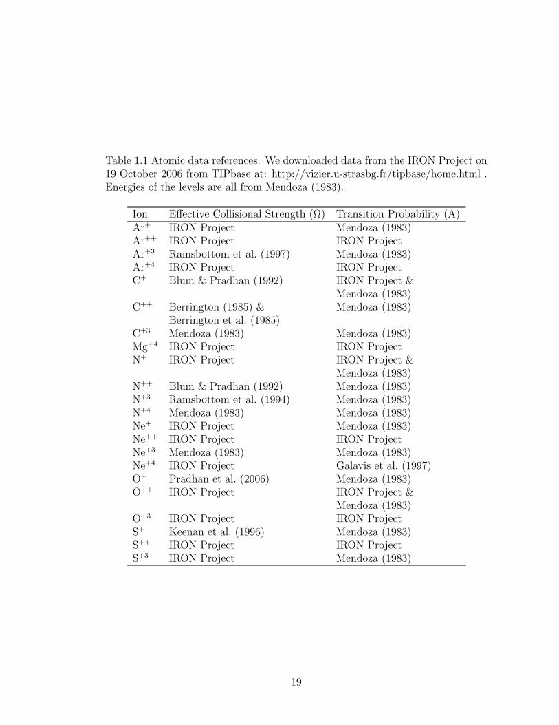
Table 1.1 Atomic data references. We downloaded data from the IRON Project on19 October 2006 from TIPbase at: http://vizier.u-strasbg.fr/tipbase/home.html .Energies of the levels are all from Mendoza (1983).

Ion Effective Collisional Strength (Ω) Transition Probability (A)Ar+ IRON Project Mendoza (1983)Ar++ IRON Project IRON ProjectAr+3 Ramsbottom et al. (1997) Mendoza (1983)Ar+4 IRON Project IRON ProjectC+ Blum & Pradhan (1992) IRON Project &

Mendoza (1983)C++ Berrington (1985) & Mendoza (1983)

Berrington et al. (1985)C+3 Mendoza (1983) Mendoza (1983)Mg+4 IRON Project IRON ProjectN+ IRON Project IRON Project &

Mendoza (1983)N++ Blum & Pradhan (1992) Mendoza (1983)N+3 Ramsbottom et al. (1994) Mendoza (1983)N+4 Mendoza (1983) Mendoza (1983)Ne+ IRON Project Mendoza (1983)Ne++ IRON Project IRON ProjectNe+3 Mendoza (1983) Mendoza (1983)Ne+4 IRON Project Galavis et al. (1997)O+ Pradhan et al. (2006) Mendoza (1983)O++ IRON Project IRON Project &

Mendoza (1983)O+3 IRON Project IRON ProjectS+ Keenan et al. (1996) Mendoza (1983)S++ IRON Project IRON ProjectS+3 IRON Project Mendoza (1983)

19

lines. For example, changing the adopted Te from 10000 K to 13000 K for the PN

IC 2448 decreases the abundance of Ne++ derived from the IR [Ne III] line at 15.55

µm by 6% but decreases the abundance of Ne++ derived from the optical [Ne III]

line at 3869 A by 80%. (3) Some ions have lines in the infrared, but not in the

optical; for example, infrared spectra show the [Ne II] line which is not observable

in the optical, but this ion dominates the total elemental neon abundance in low

ionization nebulae.

1.3.4 Ionizing Radiation Field

Massive stars and active galactic nuclei produce a hard radiation field (a radiation

field which contains a large fraction of highly energetic photons) of high intensity.

The hardness of a radiation field gives information about the type of source creating

the field. Ratios of IR lines arising from ions which have ionization energies in the

ultraviolet indicate the radiation field hardness. For example, it takes 22 eV to

create Ne+ from neutral neon and 41 eV to create Ne++ from Ne+, so if the line flux

ratio F(Ne III at 15.6µm)/F(Ne II at 12.8 µm) is high, then the ionizing radiation

field is hard. Similarly it takes 23 eV to create S++ from S+ and 35 eV to create

S+3 from S++, so the line flux ratio F(S IV at 10.5 µm)/F(S III at 18.7 µm) also

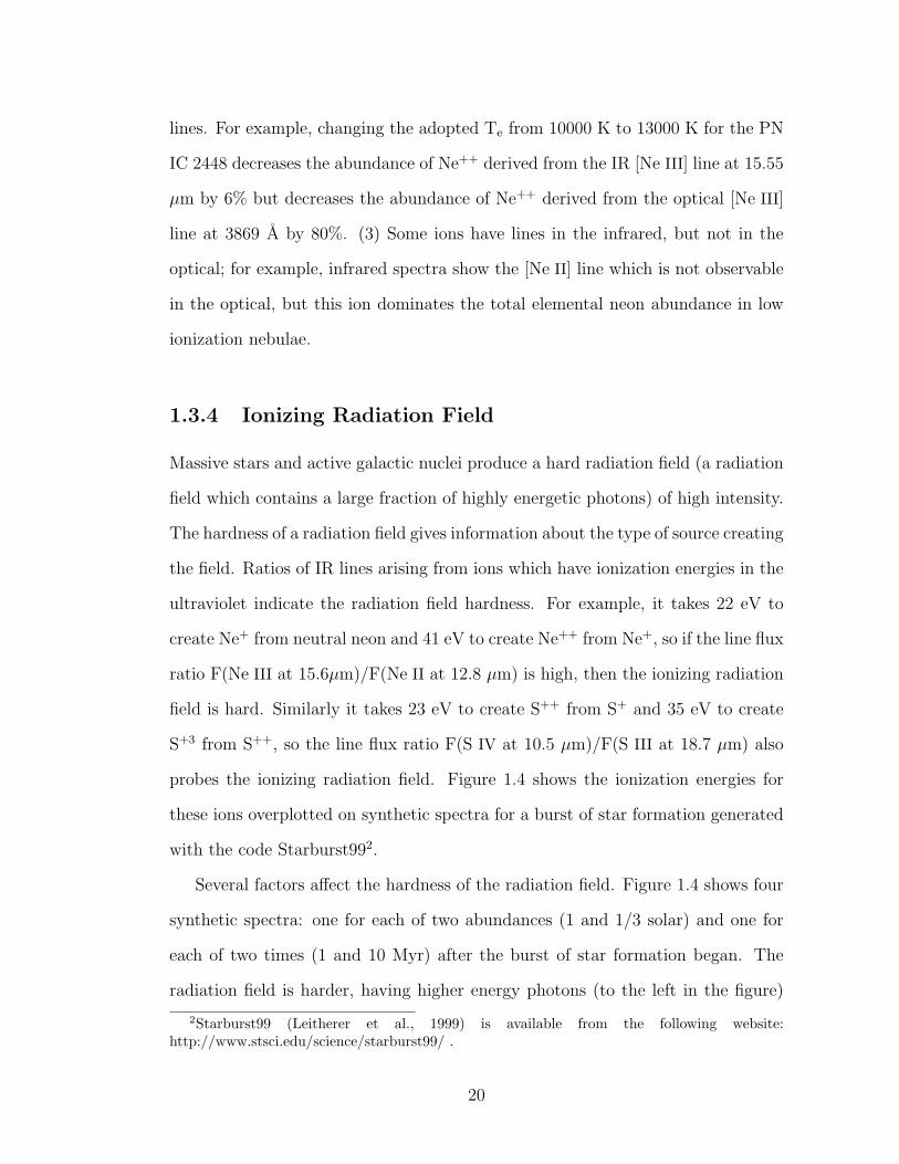
probes the ionizing radiation field. Figure 1.4 shows the ionization energies for

these ions overplotted on synthetic spectra for a burst of star formation generated

with the code Starburst992.

Several factors affect the hardness of the radiation field. Figure 1.4 shows four

synthetic spectra: one for each of two abundances (1 and 1/3 solar) and one for

each of two times (1 and 10 Myr) after the burst of star formation began. The

radiation field is harder, having higher energy photons (to the left in the figure)

2Starburst99 (Leitherer et al., 1999) is available from the following website:http://www.stsci.edu/science/starburst99/ .

20

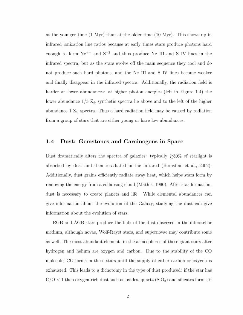
at the younger time (1 Myr) than at the older time (10 Myr). This shows up in

infrared ionization line ratios because at early times stars produce photons hard

enough to form Ne++ and S+3 and thus produce Ne III and S IV lines in the

infrared spectra, but as the stars evolve off the main sequence they cool and do

not produce such hard photons, and the Ne III and S IV lines become weaker

and finally disappear in the infrared spectra. Additionally, the radiation field is

harder at lower abundances: at higher photon energies (left in Figure 1.4) the

lower abundance 1/3 Z¯ synthetic spectra lie above and to the left of the higher

abundance 1 Z¯ spectra. Thus a hard radiation field may be caused by radiation

from a group of stars that are either young or have low abundances.

1.4 Dust: Gemstones and Carcinogens in Space

Dust dramatically alters the spectra of galaxies: typically &30% of starlight is

absorbed by dust and then reradiated in the infrared (Bernstein et al., 2002).

Additionally, dust grains efficiently radiate away heat, which helps stars form by

removing the energy from a collapsing cloud (Mathis, 1990). After star formation,

dust is necessary to create planets and life. While elemental abundances can

give information about the evolution of the Galaxy, studying the dust can give

information about the evolution of stars.

RGB and AGB stars produce the bulk of the dust observed in the interstellar

medium, although novae, Wolf-Rayet stars, and supernovae may contribute some

as well. The most abundant elements in the atmospheres of these giant stars after

hydrogen and helium are oxygen and carbon. Due to the stability of the CO

molecule, CO forms in these stars until the supply of either carbon or oxygen is

exhausted. This leads to a dichotomy in the type of dust produced: if the star has

C/O < 1 then oxygen-rich dust such as oxides, quartz (SiO2) and silicates forms; if

21

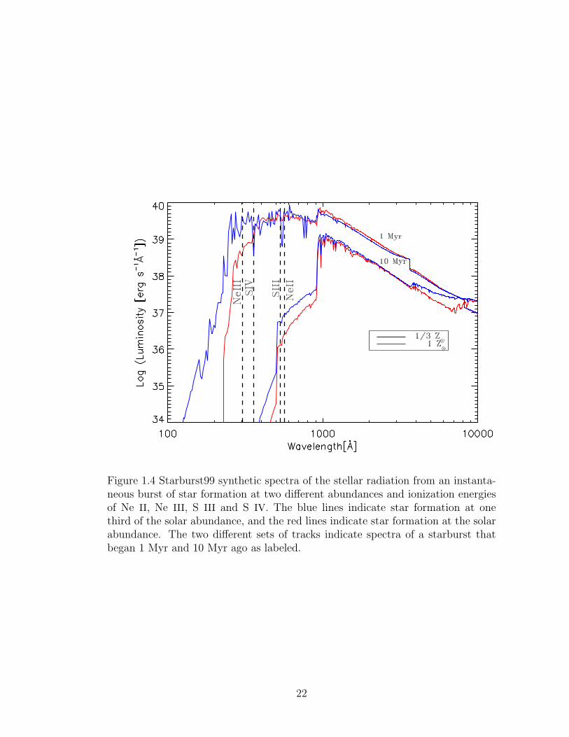
Figure 1.4 Starburst99 synthetic spectra of the stellar radiation from an instanta-neous burst of star formation at two different abundances and ionization energiesof Ne II, Ne III, S III and S IV. The blue lines indicate star formation at onethird of the solar abundance, and the red lines indicate star formation at the solarabundance. The two different sets of tracks indicate spectra of a starburst thatbegan 1 Myr and 10 Myr ago as labeled.

22

the star has C/O > 1 then carbon-rich dust such as silicon carbide (SiC), graphite,

and polycyclic aromatic hydrocarbons (PAHs) forms (Mathis, 1990). The types of

dust observed in objects discussed in this dissertation are silicates and PAHs, and

are discussed more in detail below.

1.4.1 Silicates

Amorphous silicates emit broad solid state features at ∼10 and 18 µm as well as a

broad continuum in their infrared spectra which are observable by the Spitzer IRS.

The Si-O stretching mode causes the 10 µm feature and the O-Si-O bending mode

causes the 18 µm feature. The absence of substructure in these features indicates

that the silicates are amorphous (having a disordered lattice structure) rather than

crystalline (having long-range order in the lattice structure) (Draine, 2003).

Crystalline silicates emit features beyond 20 µm. Figure 1.5 shows these crys-

talline silicate features in the continuum-subtracted IRS spectrum of one of the

Bulge PNe. Crystalline silicate features are not usually observed below 20 µm due

to the cool temperature (. 100 K) of the dust. The spectral positions of the sharp

solid state features produced by crystalline silicates imply that they are made of

molecules such as forsterite (Mg2SiO4) and enstatite (MgSiO3) and do not con-

tain much iron. Spectra in this dissertation contain features at 23.7 µm due to

forsterite, as well as complexes of features around 28 and 33 µm due to forsterite

and enstatite (Molster 2000; see Figure 1.5). Figure 1.6 shows a picture of olivine

((Mg,Fe)2SiO4), the crystalline silicate mineral found in the gemstone peridot, and

Figure 1.7 diagrams the structure of forsterite. The spectral features of amorphous

silicates are less pronounced than those of the crystalline silicates and thus it proves

more difficult to infer their chemical composition (Molster, 2000).

23

Figure 1.5 Example of crystalline silicate features in the continuum-subtractedhigh resolution IRS spectrum of the Bulge planetary nebula PNG000.7+04.7. Thecrystalline silicate features as well as the strong [S III] emission line are labeled.

Figure 1.6 Image of an olivine ((Mg,Fe)2SiO4) grain. Copyright 2004 by AndrewAlden, geology.about.com, reproduced under educational fair use, and available at:http://geology.about.com/library/bl/images/blolivine.htm.

24

2 4Forsterite ( Mg SiO )

Figure 1.7 Structure of forsterite (Mg2SiO4). The tetrahedra represent an-ions of SiO −4

4 having an O−2 anion at each vertex and a Si+4 cation in thecenter. The circles represent Mg+2 cations. Diagram designed after one at:http://www2.odn.ne.jp/7n2pmw/meteorphy2/metphys v12.htm.

1.4.2 Polycyclic Aromatic Hydrocarbons (PAHs)

PAHs are planar molecules made from building blocks of benzene rings contain-

ing six carbon atoms which are stuck together (like chicken wire) and that have

hydrogen atoms around the periphery. For example structures of these molecules

see Figure 1.8. On Earth, the incomplete combustion of carbon-containing fuels

(e.g. coal, tobacco, and incense) creates these carcinogenic PAH molecules (Leger

et al., 1987; BBC, 2001). In space, giant stars probably create most of the PAHs

as discussed above. In our Galaxy, radiation in PAH bands accounts for ∼1/7 of

the reprocessing of starlight by dust, and thus PAHs serve as significant radiative

coolants of the interstellar medium; additionally PAHs contain ∼15–20% of the

carbon in the interstellar medium (Galliano et al., 2008).

Spitzer IRS spectra of many H II regions and PNe (and other sources) show

emission from vibrational transitions in PAHs in the 5–15 µm range. Figure 1.9

shows these features in the continuum-subtracted IRS spectrum of a Bulge PN.

25

H

H

H

H

H

H

H

H H

H

H

H

H

H

C H30 14

H

H H H

H

HHH

H

H H

H

Anthanthrene

C H22 12

Figure 1.8 Example structures of PAH molecules following Allamandola et al.(1989). The vertices of the hexagons represent carbon atoms.

When a PAH molecule absorbs an energetic (UV or optical) photon, it quickly

(∼10−12–10−10 s) redistributes the energy over the vibrational modes of the PAH,

and then the PAH relaxes to the ground state by emitting IR photons over the

next seconds to hours, producing features such as the ones found at 6.2, 7.7, 8.6,

11.2, and 12.7 µm (Draine & Li, 2001; Li & Draine, 2002). A C–C stretching mode

produces the 6.2 and 7.7 µm features, a C–H in-plane bending mode causes the

8.6 µm feature, and C–H out-of-plane bending gives rise to the 11.2 and 12.7 µm

features. PAHs with sizes between twenty and forty carbon atoms are probably

the dominant emitters of these features (Allamandola et al., 1989). The type of

PAHs formed gives indications about the material from which they were made as

well as their thermal history (Leger et al., 1987).

1.5 Observing with the Spitzer Space Telescope

This dissertation employs infrared data from the Spitzer Space Telescope. It has an

85 cm diameter and was launched August 25, 2003 and is expected to have a ∼5+

26

Figure 1.9 Example of PAH features (shaded) in the continuum-subtracted IRSlow resolution spectrum of the Bulge planetary nebula PNG000.7+04.7. The PAHfeatures and the strong emission lines are labeled.

27

year lifetime. Spitzer is in an Earth-trailing solar orbit. It has three instruments:

the Infrared Array Camera, the Multiband Infrared Photometer, and the Infrared

Spectrograph (Werner et al., 2004). This dissertation mainly employs data from

the Infrared Spectrograph, and so this instrument is described in more detail below.

The Infrared Spectrograph (IRS; Houck et al., 2004) has four different modules

covering wavelengths from 5 to 38 µm. It has two low spectral resolution modules

(Short-Low (SL) and Long-Low (LL)) with R ≡ λ/∆λ ∼ 90, and it has two high

resolution modules (Short-High (SH) and Long-High (LH)) with R ∼ 600. The low

resolution modules cover the whole wavelength range of the IRS and are sensitive

to the features in the continuum (e.g. crystalline silicate and polycyclic aromatic

hydrocarbon (PAH) dust features), while the high resolution modules cover the

wavelength range 10–37 µm and are better for studying emission lines. The ob-

server may choose to blindly point the telescope with ∼1′′ positional accuracy, or

choose the PCRS or PeakUp options with 0.4′′ positional accuracy.

Spectra from Spitzer have the advantage that they are free of atmospheric ab-

sorption and the background in space is six orders of magnitude smaller than on

Earth, leading to a thousand-fold gain in sensitivity (Houck et al., 2004). Pre-

vious infrared telescope missions in space paved the way for Spitzer such as the

Infrared Astronomical Satellite (IRAS) and the Infrared Space Observatory (ISO).

ISO studied PNe in our Galaxy within a few kpc of the Sun and galactic H II re-

gions as well as some extragalactic ones. Due to its more modern detector arrays,

Spitzer has greater sensitivity than these previous IR space telescopes. Current

Spitzer studies build on this previous work; for example, Chapter 3 of this disser-

tation presents Spitzer data on eleven PNe in the Bulge of our Galaxy, a region far

enough away that it was difficult for ISO to probe the PNe there. Additionally,

the Spitzer IRS can do spectral maps, and ISO could not; Chapter 4 employs data

28

from Spitzer IRS maps of H II regions. Observations of dust features and emission

lines with the Spitzer IRS allow us to probe the physical conditions in a variety

of environments — e.g. the planetary nebulae and H II regions discussed in this

dissertation. Knowing these physical conditions is important for understanding

chemical evolution in galaxies as discussed above.

1.6 In This Dissertation

The following chapters present Spitzer IRS data on planetary nebulae and H II

regions. Specifically, Chapter 2 presents the case study of abundances in the

planetary nebula IC 2448. Chapter 3 discusses abundances and dust in eleven

planetary nebulae in the Bulge of the Galaxy. Finally, Chapter 4 gives abundance

results for H II regions across the galaxy M51.

29

CHAPTER 2

THE SPITZER IRS INFRARED SPECTRUM AND ABUNDANCES

OF THE PLANETARY NEBULA IC 2448

Paper by S. Guiles (the maiden name of S. Gutenkunst), J. Bernard-Salas,

S. R. Pottasch, & T. L. Roellig, 2007, ApJ, 660, 1282

2.1 Abstract

We present the mid-infrared spectrum of the planetary nebula IC 2448. In order to

determine the chemical composition of the nebula, we use the infrared line fluxes

from the Spitzer spectrum along with optical line fluxes from the literature and ul-

traviolet line fluxes from archival IUE spectra. We determine an extinction of CHβ

= 0.27 from hydrogen recombination lines and the radio to Hβ ratio. Forbidden

line ratios give an electron density of 1860 cm−3 and an average electron temper-

ature of 12700 K. The use of infrared lines allows us to determine more accurate

abundances than previously possible because abundances derived from infrared

lines do not vary greatly with the adopted electron temperature and extinction,

and additional ionization stages are observed. Elements left mostly unchanged by

stellar evolution (Ar, Ne, S, and O) all have subsolar values in IC 2448, indicating

that the progenitor star formed out of moderately metal deficient material. Evi-

dence from the Spitzer spectrum of IC 2448 supports previous claims that IC 2448

is an old nebula formed from a low mass progenitor star.

2.2 Introduction

Determining accurate abundances of planetary nebulae (PNe) is important for

understanding how stars and galaxies evolve (Kaler, 1985). PNe abundances of

elements made in low and intermediate mass stars (such as helium, carbon, and

30

nitrogen) can be used to test stellar evolution models (Kwok, 2000). Abundances

of elements which are not changed during evolution of low and intermediate mass

stars (such as neon, argon, sulfur, and in some cases oxygen), can give insight into

the chemical content of the gas from which the progenitor star formed (Kwok,

2000); thus abundances of PNe dispersed throughout a galaxy can be used to test

galactic evolution models.

IC 2448 is an elliptical, average sized PN located at RA = 09h07m06s.26,

DEC = −6956′30′′.7 (J2000.0, Kerber et al. (2003)). Optical emission line images

of IC 2448 show that diffuse [N II] and [O III] emission pervade the same oval re-

gion, which agrees with IC 2448 being an old, evolved nebula (Palen et al., 2002).

McCarthy et al. (1990) give further evidence for IC 2448’s advanced age, finding

that its evolutionary age is 8400 years and its dynamical age is 7000 years. IC 2448

has an Hα diameter of 10.′′7 x 10.′′0 (Tylenda et al., 2003). Thus at a distance of

2.1 ± 0.6 kpc (Mellema, 2004), IC 2448 has an Hα size of 0.11 x 0.10 pc.

Two optical surveys and one optical+ultraviolet survey of PNe include abun-

dance determinations for IC 2448 (Torres-Peimbert & Peimbert, 1977; Milingo

et al., 2002a; Kingsburgh & Barlow, 1994). Here we report the first use of mid-

infrared line fluxes from IC 2448 to determine its abundances. Using infrared (IR)

lines to derive abundances has several advantages over using optical or ultraviolet

(UV) lines (Rubin et al., 1988; Pottasch & Beintema, 1999). First, the correction

for extinction in the IR is smaller than in the optical and UV, and therefore errors

in the extinction coefficient and law affect IR line fluxes less. Second, IR lines are

less sensitive to uncertainties in the electron temperature because they come from

levels close to the ground level. Finally, some ions have lines in the IR spectrum of

IC 2448, but not in the optical or UV spectra. When combined with ionic lines of

these elements observed in the optical and UV, we have line fluxes for more ions of

31

these elements than previous studies, reducing the need for ionization correction

factors (ICFs) to account for unseen ionization stages.

In this paper we use the Spitzer IR spectrum supplemented by the optical and

UV spectra to derive ionic and total element abundances of He, Ar, Ne, S, O, N,

and C in IC 2448. The next section describes the Spitzer observations and the data

reduction. §2.4 gives the optical and UV data. In §2.5 we derive the extinction,

electron density, electron temperature, and ionic and total element abundances.

§2.6 compares the abundances of IC 2448 with solar and discusses the nature of

the progenitor star and we conclude in §2.7.

2.3 Spitzer Observations and Data Reduction

IC 2448 was observed with all four modules (Short-Low (SL), Long-Low (LL),

Short-High (SH), and Long-High (LH)) of the Infrared Spectrograph (IRS) (Houck

et al., 2004) on the Spitzer Space Telescope (Werner et al., 2004) as part of the

GTO program ID 45. The AORkeys for IC 2448 are 4112128 (SL, SH, LH observed

2004 July 18), 4112384 (SL, SH, LH off positions observed 2004 July 18), and

12409088 (LL observed 2005 February 17). The data were taken in ‘staring mode’

which acquires spectra at two nod positions along each IRS slit. For the on target

AORkeys (4112128 and 12409088), the telescope was pointed at RA = 09h07m06s.4,

DEC = −6956′31′′ (J2000.0). For the off target AORkey (4112384), the telescope

was pointed at RA = 09h07m06s.6, DEC = −6958′29′′ (J2000.0). Peak-up imaging

was performed for AORkey 4112128, but not for the other AORkeys.

The data were processed through version s14.0 of the Spitzer Science Center’s

pipeline. We begin our analysis with the unflatfielded (droopres) images to avoid

potential problems in the flatfield. Then we run the irsclean1 program to remove

1Program available from the Spitzer Science Center’s website at http://ssc.spitzer.caltech.edu

32

rogue and flagged pixels, using a mask of rogue pixels from the same campaign as

the data. Next we remove the background. To do this we use the off positions

for SL, SH, and LH; for LL we use the off order (for example, LL1 nod1 - LL2

nod1). The high resolution spectra (SH and LH) are extracted from the images

using a scripted version of the SMART program (Higdon et al., 2004), using full-slit

extraction. Due to the extended nature of IC 2448, the low resolution spectra (SL

and LL) are extracted from the images manually in SMART using a fixed column

extraction window of width 14.0 pixels (25.′′2) for SL and 8.0 pixels (40.′′8) for

LL. The spectra are calibrated by multiplying by the relative spectral response

function which is created by dividing the template of a standard star (HR 6348

for SL and LL, and ξ Dra for SH and LH) by the spectrum of the standard star

extracted in the same way as the source (Cohen et al. (2003); G. C. Sloan, private

communication). Spikes due to deviant pixels missed by the irsclean program are

removed manually.

The large aperture LH (11′′.1 x 22′′.3) and LL (10′′.5 x 168′′) slits are big

enough to contain all of the flux from IC 2448. This is supported by the fact that

the continuum flux from IC 2448 in LH matches that from LL with no scaling

between them. However, the smaller aperture SH (4′′.7 x 11′′.3) and SL (3′′.6 x

57′′) slits are too small to contain the entire object. Thus we scale SL up to LL

and SH up to LH. SL has a scaling factor of 2.30 and SH has a scaling factor of

3.00. No scaling factor is needed for orders within a module (for example, SL1,

SL2, and SL3 all have the same scaling factor of 2.30). Additionally, there is no

need of a scaling factor between the two nod positions.

Figure 2.1 shows the average of the two nods of the Spitzer IRS spectrum of

IC 2448. The peak of the continuum at ∼30 µm in Fλ units implies that the dust is

cool, ∼100 K. No evidence of polycyclic aromatic hydrocarbons (PAHs) or silicate

33

dust is seen in the spectrum. We see lines from ions of H, Ar, Ne, S and O in

the IR spectrum of IC 2448. Close-ups of the lines in the high resolution Spitzer

IRS spectrum of IC 2448 are shown in Figure 2.2. High ionization lines of [O IV]

(ionization potential IP = 55 eV) and [Ar V] (IP = 60 eV) are observed, but even

higher ionization lines such as [Ne V] (IP = 97 eV) and [Mg V] (IP = 109 eV) are

not observed, indicating that there is only a moderately hard radiation field. Low

ionization lines that would come from the photodissociation region (PDR) such as

[Ar II] (IP = 16 eV) and [Si II] (IP = 8 eV) are not observed. A complete list of the

observed lines and their fluxes is given in Table 2.1. The highest flux lines in the

SH module (10.51 µm[S IV] and 15.55 µm[Ne III]) have bumps on each side of them

that are instrumental artifacts, possibly resulting from internal reflection in the SH

module or an effect of photon-responsivity. The bumps are just visible in Figure

2.2 for the [S IV] line. However, the bumps contain a negligible amount of flux –

only ∼3% and ∼1% of the flux in the main [S IV] and [Ne III] lines respectively,

and we did not include these small contributions in our line flux measurements.

The line fluxes are measured interactively in SMART for each nod position by

performing a linear fit to the continuum on both sides of the line and then fitting a

gaussian to the line. The values of the average line fluxes from both nod positions

are given in Table 2.1. We estimate uncertainties in the line fluxes in two ways.

In the first method, we propagate the uncertainties in the gaussian fit to the line

flux to determine the uncertainty on the average flux from both nod positions.

In the second method, we use the standard deviation of the fluxes measured in

the two nod positions to determine the uncertainty on the average flux from both

nod positions. We then take the final uncertainty as the greater of these two

uncertainties. Lines fluxes typically have uncertainties . 10%; lines with larger

uncertainties (. 15% and . 30%) are marked in Table 2.1. We determine 3σ upper

34

Figure 2.1 The scaled, nod averaged, Spitzer IRS spectrum of IC 2448. The lowresolution spectrum is shown in black and the high resolution spectrum in grey. SLis scaled up to LL, and SH is scaled up to LH because SL and SH both have smallapertures that do not receive the entire flux from IC 2448. Some of the lines havepeaks above 5 Jy (the strongest line, O IV at 25.89 µm, peaks at 270 Jy in the HRspectrum), but the y-axis range is restricted in the plot to reveal the continuum.

limits for lines not observed but relevant for the abundance analysis (denoted by

a less-than sign in Table 2.1). Upper limits are obtained by calculating the flux

contained in a gaussian with width determined by the instrument resolution and

height equal to three times the root mean square (RMS) deviation in the spectrum

at the wavelength of the line.

35

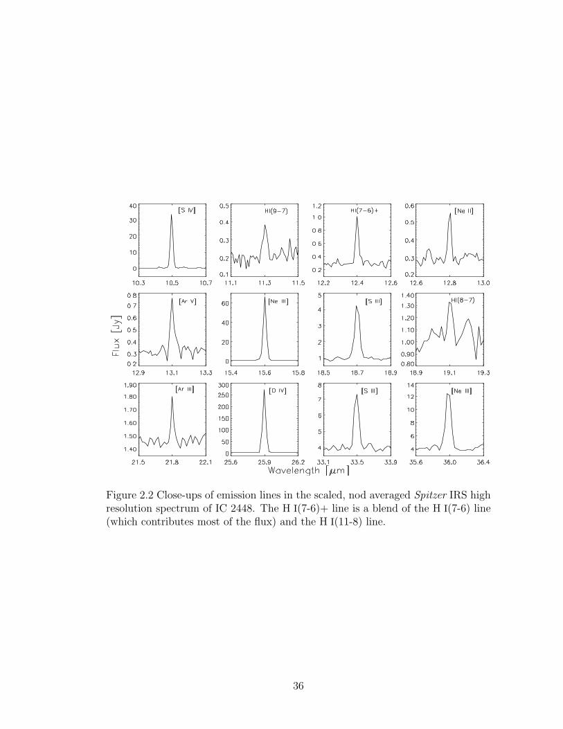
Figure 2.2 Close-ups of emission lines in the scaled, nod averaged Spitzer IRS highresolution spectrum of IC 2448. The H I(7-6)+ line is a blend of the H I(7-6) line(which contributes most of the flux) and the H I(11-8) line.

36

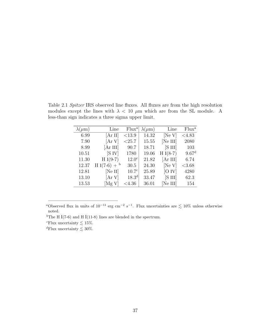
Table 2.1 Spitzer IRS observed line fluxes. All fluxes are from the high resolutionmodules except the lines with λ < 10 µm which are from the SL module. Aless-than sign indicates a three sigma upper limit.

λ(µm) Line Fluxa λ(µm) Line Fluxa

6.99 [Ar II] <13.9 14.32 [Ne V] <4.837.90 [Ar V] <25.7 15.55 [Ne III] 20808.99 [Ar III] 90.7 18.71 [S III] 103

10.51 [S IV] 1780 19.06 H I(8-7) 9.67d

11.30 H I(9-7) 12.0c 21.82 [Ar III] 6.7412.37 H I(7-6) + b 30.5 24.30 [Ne V] <3.6812.81 [Ne II] 10.7c 25.89 [O IV] 428013.10 [Ar V] 18.3d 33.47 [S III] 62.313.53 [Mg V] <4.36 36.01 [Ne III] 154

aObserved flux in units of 10−14 erg cm−2 s−1. Flux uncertainties are . 10% unless otherwisenoted.

bThe H I(7-6) and H I(11-8) lines are blended in the spectrum.cFlux uncertainty . 15%.dFlux uncertainty . 30%.

37

2.4 Optical and UV Data

We complement our IR line fluxes with optical and UV line fluxes in order to deter-

mine abundances. The optical and UV data provide line fluxes from ions not seen

in the infrared spectrum (especially carbon and nitrogen). We obtain optical line

fluxes from Milingo et al. (2002b). They observed IC 2448 with the 1.5 m telescope

and Cassegrain spectrograph at the Cerro Tololo Inter-American Observatory in

the Spring of 1997 using a 5 ′′x 320′′ slit. The slit width is about half of the diam-

eter of IC 2448, and so Milingo et al. (2002b) missed some of the nebular flux. We

assume that the optical lines measured in the small aperture are representative of

the entire nebula of IC 2448 because IC 2448 has evenly distributed optical [N II]

and [O III] line emission (Palen et al., 2002). The extinction corrected fluxes for

the lines we use are listed in Table 2.2 as given by Milingo et al. (2002b). These

authors report uncertainties in their line fluxes of . 10% for their strong lines

(with strengths ≥ Hβ) and have flagged uncertainties of & 25% and & 50% for the

weaker lines. These uncertainties are given in Table 2.2.

High and low resolution large aperture International Ultraviolet Explorer (IUE)

spectra of IC 2448 from the IUE Newly Extracted Spectra (INES) system are

available on the web2. The high resolution spectra we use are labeled SWP19067

and LWR15096, and the low resolution spectra we use are labeled SWP03194 and

LWR02756. We use SMART to measure the line fluxes from the spectra, and the

results are listed in Table 2.3. Uncertainties are obtained from the gaussian fit to

each line and are . 15% unless otherwise noted. The IUE large aperture (10′′x

23′′ ellipse) is big enough to contain essentially all of the flux from IC 2448, and

no aperture scaling factor needs to be applied to the spectra.

2The IUE INES system archive website is http://ines.vilspa.esa.es

38

Table 2.2 Extinction corrected optical line fluxes relative to Hβ=100 from Milingoet al. (2002b)

λ (A) Line Fluxa λ (A) Line Fluxa

3727 [O II] 5.1b 6584 [N II] 1.03869 [Ne III] 103 6717 [S II] 0.14070 [S II] 1.1 6731 [S II] 0.14363 [O III] 16.4 7005 [Ar V] 0.14471 He I 3.3 7135 [Ar III] 4.84686 He II 40.3 7236 [Ar IV] 0.1c

4740 [Ar IV] 4.7 7264 [Ar IV] 0.1c

4959 [O III] 386 7323 [O II] 0.65007 [O III] 1173 7751 [Ar III] 1.25755 [N II] 0.1b 9069 [S III] 2.56312 [S III] 0.5 9532 [S III] 5.26436 [Ar V] 0.1b

aExtinction corrected flux relative to Hβ=100. The Hβ flux in the same aperture is 724.4 × 10−14

erg cm−2 s−1 (Milingo et al., 2002b). Flux uncertainties are . 10% unless otherwise noted.bFlux uncertainty & 50%.cFlux uncertainty & 25%.

Table 2.3 Selected observed ultraviolet line fluxes

λ (A) Line Fluxa λ (A) Line Fluxa

1241 N V 8.86b 1907 C III] 22501483 N IV] 58.5b 2326 C II] 12.6b,c

1548 C IV 1900 2422 [Ne IV] 1841640 He II 2180 2471 [O II] 4.77b,d

1750 N III] 75.5

aObserved flux in units of 10−14 erg cm−2 s−1. Unless otherwise marked, all fluxes are from IUElow resolution spectra and have uncertainties of . 15%.

bFlux from IUE high resolution spectra.cFlux uncertainty . 50%.dFlux uncertainty . 30%.

39

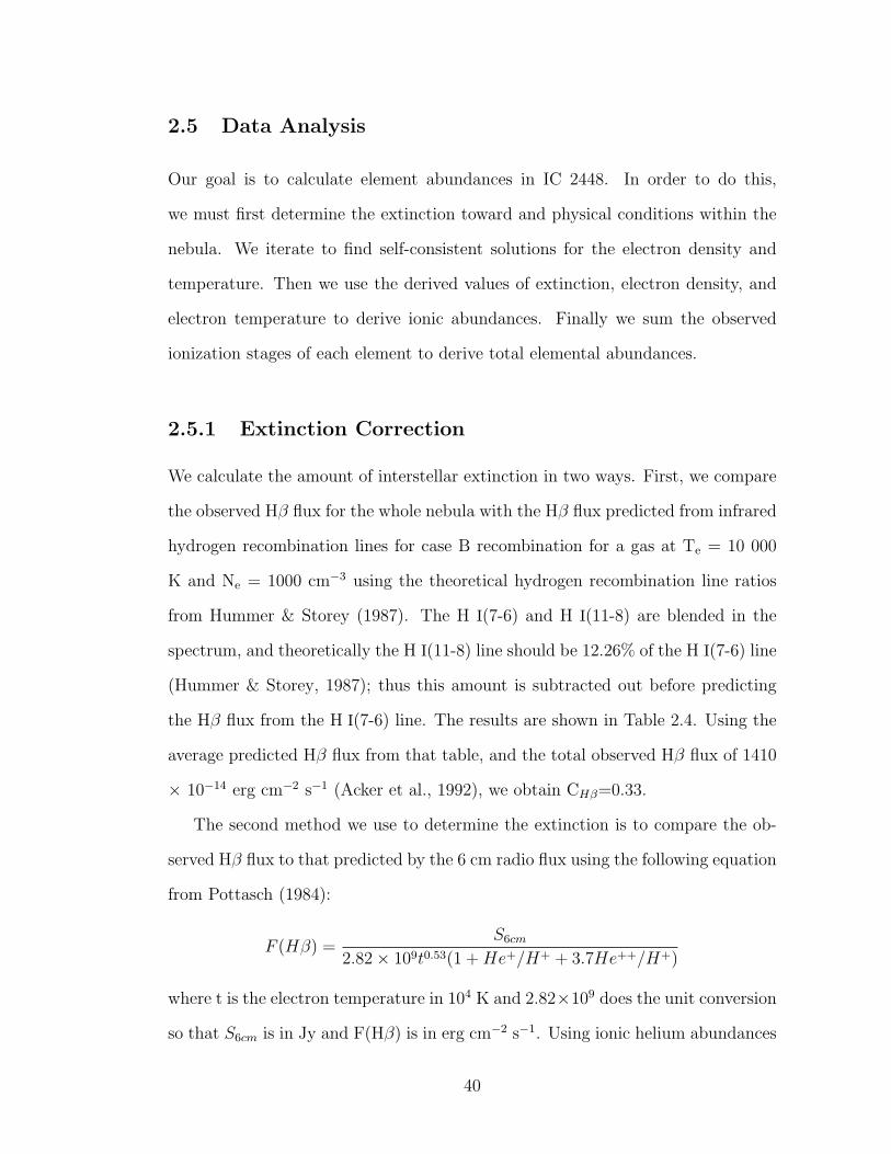
2.5 Data Analysis

Our goal is to calculate element abundances in IC 2448. In order to do this,

we must first determine the extinction toward and physical conditions within the

nebula. We iterate to find self-consistent solutions for the electron density and

temperature. Then we use the derived values of extinction, electron density, and

electron temperature to derive ionic abundances. Finally we sum the observed

ionization stages of each element to derive total elemental abundances.

2.5.1 Extinction Correction

We calculate the amount of interstellar extinction in two ways. First, we compare

the observed Hβ flux for the whole nebula with the Hβ flux predicted from infrared

hydrogen recombination lines for case B recombination for a gas at Te = 10 000

K and Ne = 1000 cm−3 using the theoretical hydrogen recombination line ratios

from Hummer & Storey (1987). The H I(7-6) and H I(11-8) are blended in the

spectrum, and theoretically the H I(11-8) line should be 12.26% of the H I(7-6) line

(Hummer & Storey, 1987); thus this amount is subtracted out before predicting

the Hβ flux from the H I(7-6) line. The results are shown in Table 2.4. Using the

average predicted Hβ flux from that table, and the total observed Hβ flux of 1410

× 10−14 erg cm−2 s−1 (Acker et al., 1992), we obtain CHβ=0.33.

The second method we use to determine the extinction is to compare the ob-

served Hβ flux to that predicted by the 6 cm radio flux using the following equation

from Pottasch (1984):

F (Hβ) =S6cm

2.82× 109t0.53(1 + He+/H+ + 3.7He++/H+)

where t is the electron temperature in 104 K and 2.82×109 does the unit conversion

so that S6cm is in Jy and F(Hβ) is in erg cm−2 s−1. Using ionic helium abundances

40

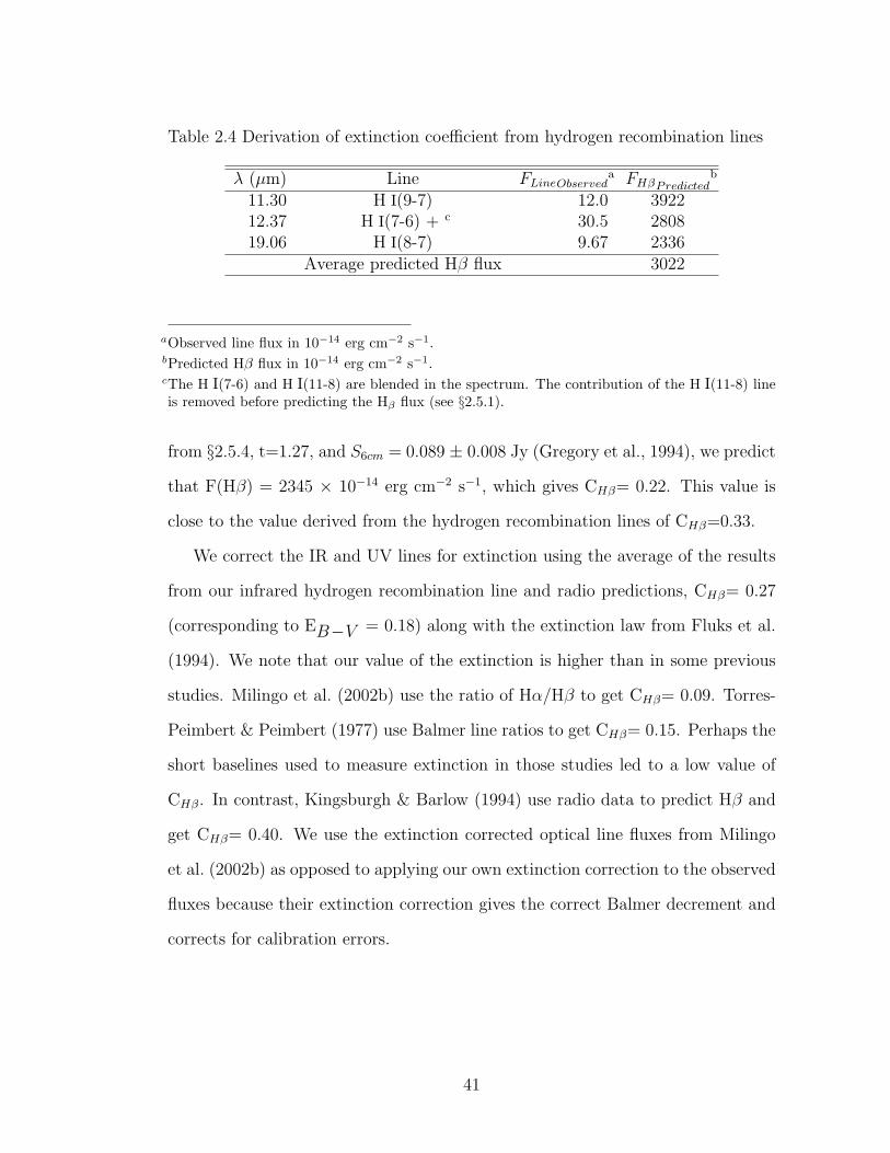
Table 2.4 Derivation of extinction coefficient from hydrogen recombination lines

λ (µm) Line FLineObserveda FHβPredicted

b

11.30 H I(9-7) 12.0 392212.37 H I(7-6) + c 30.5 280819.06 H I(8-7) 9.67 2336

Average predicted Hβ flux 3022

aObserved line flux in 10−14 erg cm−2 s−1.bPredicted Hβ flux in 10−14 erg cm−2 s−1.cThe H I(7-6) and H I(11-8) are blended in the spectrum. The contribution of the H I(11-8) lineis removed before predicting the Hβ flux (see §2.5.1).

from §2.5.4, t=1.27, and S6cm = 0.089 ± 0.008 Jy (Gregory et al., 1994), we predict

that F(Hβ) = 2345 × 10−14 erg cm−2 s−1, which gives CHβ= 0.22. This value is

close to the value derived from the hydrogen recombination lines of CHβ=0.33.

We correct the IR and UV lines for extinction using the average of the results

from our infrared hydrogen recombination line and radio predictions, CHβ= 0.27

(corresponding to EB−V = 0.18) along with the extinction law from Fluks et al.

(1994). We note that our value of the extinction is higher than in some previous

studies. Milingo et al. (2002b) use the ratio of Hα/Hβ to get CHβ= 0.09. Torres-

Peimbert & Peimbert (1977) use Balmer line ratios to get CHβ= 0.15. Perhaps the

short baselines used to measure extinction in those studies led to a low value of

CHβ. In contrast, Kingsburgh & Barlow (1994) use radio data to predict Hβ and

get CHβ= 0.40. We use the extinction corrected optical line fluxes from Milingo

et al. (2002b) as opposed to applying our own extinction correction to the observed

fluxes because their extinction correction gives the correct Balmer decrement and

corrects for calibration errors.

41

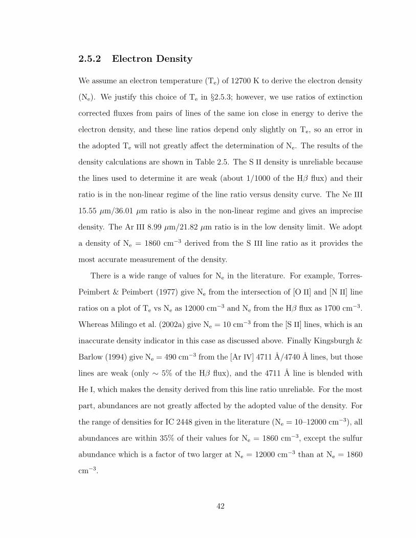
2.5.2 Electron Density

We assume an electron temperature (Te) of 12700 K to derive the electron density

(Ne). We justify this choice of Te in §2.5.3; however, we use ratios of extinction

corrected fluxes from pairs of lines of the same ion close in energy to derive the

electron density, and these line ratios depend only slightly on Te, so an error in

the adopted Te will not greatly affect the determination of Ne. The results of the

density calculations are shown in Table 2.5. The S II density is unreliable because

the lines used to determine it are weak (about 1/1000 of the Hβ flux) and their

ratio is in the non-linear regime of the line ratio versus density curve. The Ne III

15.55 µm/36.01 µm ratio is also in the non-linear regime and gives an imprecise

density. The Ar III 8.99 µm/21.82 µm ratio is in the low density limit. We adopt

a density of Ne = 1860 cm−3 derived from the S III line ratio as it provides the

most accurate measurement of the density.

There is a wide range of values for Ne in the literature. For example, Torres-

Peimbert & Peimbert (1977) give Ne from the intersection of [O II] and [N II] line

ratios on a plot of Te vs Ne as 12000 cm−3 and Ne from the Hβ flux as 1700 cm−3.

Whereas Milingo et al. (2002a) give Ne = 10 cm−3 from the [S II] lines, which is an

inaccurate density indicator in this case as discussed above. Finally Kingsburgh &

Barlow (1994) give Ne = 490 cm−3 from the [Ar IV] 4711 A/4740 A lines, but those

lines are weak (only ∼ 5% of the Hβ flux), and the 4711 A line is blended with

He I, which makes the density derived from this line ratio unreliable. For the most

part, abundances are not greatly affected by the adopted value of the density. For

the range of densities for IC 2448 given in the literature (Ne = 10–12000 cm−3), all

abundances are within 35% of their values for Ne = 1860 cm−3, except the sulfur

abundance which is a factor of two larger at Ne = 12000 cm−3 than at Ne = 1860

cm−3.

42

Table 2.5 Electron densities assuming Te = 12700 K. The S III lines provide themost accurate measurement of the density, and so we assume a density of 1860cm−3.

ion lines used Ioniz. Potential Line Ratio Ne

(µm) (eV) (cm−3)S II 0.6731/0.6717 10.36 1.00 781S III 18.71/33.47 23.33 1.66 1860

2.5.3 Electron Temperature

We use extinction corrected fluxes from pairs of lines of the same ion widely sep-

arated in energy to derive the electron temperature (Te) assuming an electron

density of Ne = 1860 cm−3. The results are shown in Table 2.6. It is possible to

determine Te from pairs of ionic lines not in the table (e.g. N II 5755 A/6584 A and

Ar V 7005 A/13.10 µm); however, the Te determined from those ratios is not as

accurate because one or both of the lines in each of those ratios is not high quality.

We adopt Te = 12700 K from the average of the electron temperatures in the table.

We use this value of the temperature in the subsequent abundance analysis. For

comparison, Torres-Peimbert & Peimbert (1977) give T(O III) = 12500 K. Milingo

et al. (2002a) give T(O III) = 12500 K, T(N II)=22400 K, and T(S III) = 25200

K; however, they deem the values of T(N II) and T(S III) unrealistic. Kingsburgh

& Barlow (1994) give T(O III) = 11000 K. We note that there is no correlation of

Te with ionization potential, although such a correlation has been noticed in some

previous studies (e.g. Pottasch & Beintema (1999); Bernard-Salas et al. (2001)).

2.5.4 Abundances

We use the Ne and Te given above together with the IR, optical, and UV extinction

corrected line fluxes to determine the ionic abundances for ions of Ar, Ne, S,

43

Table 2.6 Electron temperatures assuming Ne = 1860 cm−3

ion lines used Ioniz. Potential Line Ratio Te

(µm) (eV) (K)S III 0.6312/18.71 23.33 0.125 13900Ar III 0.7751/8.99 27.63 0.334 11500O III 0.4363/0.5007 35.12 0.0140 13100Ne III 0.3869/15.55 40.96 1.27 12400

Table 2.7 Ionic and elemental abundances

Ion λ (µm) Nion/NH+ Nelem/NH+

He+ 0.4471 0.060He++ 0.4686 0.034 0.094Ar+ a 6.99 <4.21×10−08

Ar++ 8.99, 21.82 3.57×10−07

Ar3+ 0.4740 7.73×10−07

Ar4+ 13.10 1.82×10−08 1.15×10−06

Ne+ 12.81 5.24×10−07

Ne++ 15.55 4.96×10−05

Ne3+ 0.2422 1.41×10−05

Ne4+ 24.30 <1.31×10−08 6.42×10−05

S++ 18.71, 33.47 4.15×10−07

S3+ 10.51 1.53×10−06 1.95×10−06

O+ 0.7323 2.82×10−06

O++ 0.4363, 0.4959, 0.5007 2.10×10−04

O3+ 25.89 3.86×10−05 2.51×10−04

N+ 0.6584 1.20×10−07

N++ 0.1750 2.39×10−05

N3+ 0.1483 3.09×10−05

N4+ b 0.1241 4.20×10−06 5.49×10−05

C+ 0.2326 2.09×10−06

C++ 0.1907 1.64×10−04

C3+ 0.1548 1.05×10−04 2.71×10−04

aAr+ may originate from the PDR (instead of the ionized region). However, it does not affect thetotal argon abundance because the upper limit is small compared to abundances of other argonions.

bN4+ probably originates from the star and thus it is not included in the total nitrogen abundance.

44

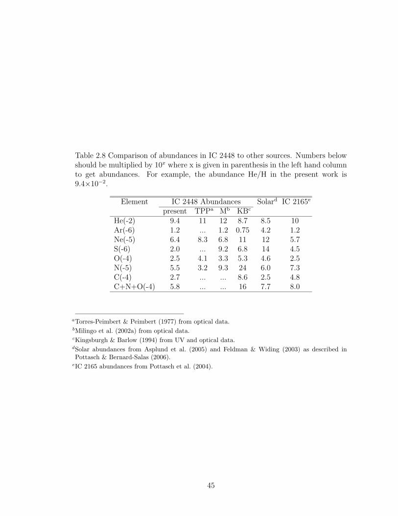
Table 2.8 Comparison of abundances in IC 2448 to other sources. Numbers belowshould be multiplied by 10x where x is given in parenthesis in the left hand columnto get abundances. For example, the abundance He/H in the present work is9.4×10−2.

Element IC 2448 Abundances Solard IC 2165e

present TPPa Mb KBc

He(-2) 9.4 11 12 8.7 8.5 10Ar(-6) 1.2 ... 1.2 0.75 4.2 1.2Ne(-5) 6.4 8.3 6.8 11 12 5.7S(-6) 2.0 ... 9.2 6.8 14 4.5O(-4) 2.5 4.1 3.3 5.3 4.6 2.5N(-5) 5.5 3.2 9.3 24 6.0 7.3C(-4) 2.7 ... ... 8.6 2.5 4.8C+N+O(-4) 5.8 ... ... 16 7.7 8.0

aTorres-Peimbert & Peimbert (1977) from optical data.bMilingo et al. (2002a) from optical data.cKingsburgh & Barlow (1994) from UV and optical data.dSolar abundances from Asplund et al. (2005) and Feldman & Widing (2003) as described inPottasch & Bernard-Salas (2006).

eIC 2165 abundances from Pottasch et al. (2004).

45

O, N, and C. The helium ionic abundances are calculated using emissivities in

Benjamin et al. (1999). Then we sum the ionic abundances for all expected stages

of ionization of an element to determine the abundance of that element. The S+

probably originates in the PDR because it has an IP of 10.4 eV; thus it is not

included in the total sulfur abundance. The N4+ 1241 A line probably originates

from the star because no other ions with such large ionization potentials (IP =

77.7 eV) are observed; thus it is not included in the total nitrogen abundance.

The infrared spectrum enables us to observe lines of Ar4+, Ne+, S3+, and O3+

that are missing or weak in the combined optical and UV spectrum of IC 2448;

and it additionally allows us to place upper limits on the amount of Ar+ and Ne4+.

Observations of the S3+ and O3+ infrared lines are particularly important for deter-

mining accurate elemental abundances because those ionization stages contribute

significantly to the total sulfur and oxygen elemental abundances respectively. The

results for ionic and total element abundances are shown in Table 2.7. We do not

need to apply an ionization correction factor (ICF) because we observe all ioniza-

tion stages expected to have a significant contribution to the elemental abundances

derived here.

One might expect S4+ to be present in the H II region because ions with higher

ionization potentials are observed. However, a model of the PN Me 2-1, which

has a star with similar temperature to IC 2448’s central star, indicates that the

S4+ contribution to the total sulfur abundance is ∼ 15%. S4+ is not important

because photons with enough energy to ionize S3+ to S4+ are absorbed by the

more abundant ions of other elements that have similar ionization potentials (R.

Surendiranath, private communication). We assume that the S4+ contribution to

the total sulfur abundance is negligible, and so we do not use an ICF for sulfur.

46

2.6 Discussion

In Table 2.8 we compare the abundances we derive with those from previous works.

Our helium, argon and neon abundances are all close to previous results. For the

remaining elements, we discuss reasons why our results differ from previous ones

below. The abundances of Ar, Ne, S, and O determined in this study should be

more accurate and precise than in previous studies because we have used infrared

lines that are less sensitive to temperature and extinction than optical and UV

lines.

The sulfur abundance determined in this study is lower than previously re-

ported. Milingo et al. (2002a) used an ICF of 39.18 to account for unseen S3+,

and such a large ICF leads to a large uncertainty in their sulfur abundance result.

Kingsburgh & Barlow (1994) used an ICF of 3.13 to account for unseen S2+ and

S3+. Therefore, while we report a lower sulfur abundance than previous authors,

it is more accurate because we observe both S2+ and S3+ in the IR spectrum and

thus we do not need to use an ICF.

The oxygen abundance derived here is somewhat lower than given in former

studies. This is mainly due to our use of the O3+ 25.89 µm line to determine the

O3+ abundance, because the ICFs of previous studies overestimated the amount of

O3+. We find that the O3+ abundance is only 15% of the total oxygen abundance,

while ICFs used in previous studies assume that O3+ contributes between 42% and

57% of the total oxygen abundance.

The nitrogen and carbon abundances determined here and in previous studies

are uncertain. The nitrogen abundances determined from the two optical studies

have large uncertainties because the optical studies must use large ICFs (Torres-

Peimbert & Peimbert (1977) use 33.9 and Milingo et al. (2002a) use 1279.69) to

account for unseen N++, N3+, and N4+. This study and that of Kingsburgh &

47

Barlow (1994) use UV lines for important ionization stages that dominate the

element abundances of nitrogen and carbon. However, the ionic abundances de-

termined from UV lines are very sensitive to the adopted electron temperature

and extinction. For example, lowering (raising) the adopted Te by just 1000 K

leads to an increase of ∼70% (decrease of ∼40%) in the derived nitrogen and car-

bon abundances. Lowering (raising) the adopted CHβ by 0.10 leads to up to a

∼30% decrease (increase) in the derived nitrogen and carbon abundances. We use

a higher Te than Kingsburgh & Barlow (1994) (we use Te=12700 K and they use

Te=11000 K), and we use a lower extinction (we use CHβ=0.27 whereas they use

CHβ=0.40). Increasing the temperature and decreasing the extinction both have

the effect of lowering the abundances derived from UV lines, causing the nitrogen

and carbon element abundances derived in this study to be less than those derived

by Kingsburgh & Barlow (1994).

The average of the Ar, Ne, and O abundances gives a metallicity of ∼0.45 Z¯,

with an uncertainty of roughly 30%. These elements are left relatively unchanged

during stellar evolution. Thus their low abundances imply that IC 2448’s progen-

itor star formed from metal deficient material, with a metallicity closer to that of

the large magellanic cloud than to that of the sun. Sulfur is also left relatively

unchanged during stellar evolution. However, many PNe have low sulfur abun-

dances compared to solar, and so the sulfur abundance is not used in the average

metallicity calculation. The sulfur abundance of IC 2448 is lower than the sul-

fur abundances of all 26 of the PNe studied by Pottasch & Bernard-Salas (2006),

which supports the idea of a subsolar composition for IC 2448’s progenitor star.

The abundance of helium derived here for IC 2448 is somewhat above solar, which

implies that some chemical processing took place within IC 2448’s progenitor star.

The nitrogen and carbon abundances are more uncertain, but close to solar.

48

Mendez et al. (1992) use their determinations of IC 2448’s stellar gravity (log

g = 4.8) and effective temperature (Teff = 65000 K) to derive the current mass

of IC 2448’s star as 0.58 M¯. This current stellar mass corresponds to an initial

stellar mass of Mi ≈ 1 M¯ at a metallicity of Z = 0.5-1.0 Z¯ (Vassiliadis & Wood,

1993). This low stellar mass, along with the low metallicity of IC 2448’s progenitor

star, imply that the first and perhaps the third dredge-up occurred.

First dredge-up would have increased the abundances of 4He, 14N, and 13C,

decreased the abundance of 12C, and left the 16O abundance the same (Marigo

et al., 2003). Second dredge-up (which increases 4He and 14N but decreases 12C,

13C, and 16O) is only expected to occur if the initial mass of the progenitor star is

between 3 and 5 M¯ (Marigo et al., 2003), and so it is not expected to occur here.

Third dredge-up, which significantly increases 4He and 12C and slightly increases

the amounts of some other elements (Marigo et al., 2003), might have occurred.

It is expected to occur in stars that have Mi & 1.5 M¯ at Z = Z¯, but this limit

is at lower masses for lower Z (Marigo et al., 1999). Third dredge-up enriches the

amount of carbon relative to oxygen, and thus a C/O ratio greater than one would

indicate that third dredge-up occurred (Iben & Renzini, 1983).

The C/O ratio in IC 2448 derived here is 1.1, but the carbon abundance of

IC 2448 is very uncertain as discussed above. Thus we cannot determine if the

C/O ratio is really greater or less than one. The IR spectrum of IC 2448 (Figure

2.1) does not show PAHs which are often observed in PNe with C/O > 1, nor

does it show silicates which are often observed in PNe with C/O < 1 (Zuckerman

& Aller, 1986; Bernard-Salas & Tielens, 2005). The uncertainty in our carbon

abundance and the lack of PAHs and silicates in the IR spectrum do not allow us

to determine if IC 2448 is carbon-rich or oxygen-rich.

The abundances of IC 2448 are close to the abundances of PN IC 2165 which

49

is a spherical nebula with a low mass (. 3 M¯) progenitor star (Pottasch et al.,

2004). IC 2165 probably experienced third dredge-up (in addition to first dredge-

up) because it has C/O ∼ 2 (Pottasch et al., 2004). The elements not much affected

by the various dredge-up episodes (Ar, Ne, S, and O) all have subsolar values in

IC 2448 and IC 2165, which implies that the progenitor stars of these nebula were

created from metal deficient gas.

The IR continuum of IC 2448 gives a cool dust temperature of∼ 100 K, support-

ing previous studies that show IC 2448 to be an old, evolved nebula. Additionally,

IR lines that would come from the photodissociation region such as [Ar II] and

[Si II] are not observed. Perhaps this indicates that most of the photodissociation

region has been destroyed, which fits the picture of IC 2448 being an old PN where

the ionization front has gobbled up most of the photodissociation region.

2.7 Conclusions

This is the first mid-IR spectral study of IC 2448. The abundance of helium is

slightly above solar, indicating that some chemical enrichment has occurred. The

high uncertainties in the nitrogen and carbon abundances (due to their reliance

on abundances determined from UV lines which depend strongly on the electron

temperature and to a lesser extent on the extinction) make it difficult to determine

how much chemical enrichment occurred. The elements not affected much by stellar

evolution (Ar, Ne, S, and O) all have subsolar values in IC 2448, indicating that

the progenitor star formed out of somewhat metal deficient material. Our use of

infrared ionic lines which are less sensitive to extinction and temperature, and some

of which arise from ions with no observable lines in the optical or UV, leads to a

more accurate determination of abundances for Ar, Ne, S, and O than previously

possible. The abundances determined fit with the picture of IC 2448 having a low

50

mass progenitor star that underwent first and perhaps third dredge-up. The IR

continuum gives a cool dust temperature of ∼ 100 K, supporting previous studies

that show IC 2448 to be an old, evolved nebula. Additionally, lines that would arise

from the PDR are missing or weak, indicating that much of the PDR is destroyed,

consistent with IC 2448 being an old PN.

This work is based in part on observations made with the Spitzer Space Tele-

scope, which is operated by the Jet Propulsion Laboratory, California Institute

of Technology under NASA contract 1407. Support for this work was provided

by NASA through Contract Number 1257184 issued by JPL/Caltec. This work

is also based in part on INES data from the IUE satellite. This research made

use of the SIMBAD database, operated at CDS, Strasbourg, France. We thank

R. Surendiranath for his comments on the contribution of S4+ to the total sulfur

abundance.

51

CHAPTER 3

CHEMICAL ABUNDANCES AND DUST IN PLANETARY

NEBULAE IN THE GALACTIC BULGE

Paper by S. Gutenkunst, J. Bernard-Salas, S. R. Pottasch, G. C. Sloan, &

J. R. Houck, accepted for publication in The Astrophysical Journal

3.1 Abstract

We present mid-infrared Spitzer spectra of eleven planetary nebulae in the Galac-

tic Bulge. We derive argon, neon, sulfur, and oxygen abundances for them using

mainly infrared line fluxes combined with some optical line fluxes from the liter-

ature. Due to the high extinction toward the Bulge, the infrared spectra allow

us to determine abundances for certain elements more accurately that previously

possible with optical data alone. Abundances of argon and sulfur (and in most

cases neon and oxygen) in planetary nebulae in the Bulge give the abundances

of the interstellar medium at the time their progenitor stars formed; thus these

abundances give information about the formation and evolution of the Bulge. The

abundances of Bulge planetary nebulae tend to be slightly higher than those in the

Disk on average, but they do not follow the trend of the Disk planetary nebulae,

thus confirming the difference between Bulge and Disk evolution. Additionally,

the Bulge planetary nebulae show peculiar dust properties compared to the Disk

nebulae. Oxygen-rich dust feature (crystalline silicates) dominate the spectra of

all of the Bulge planetary nebulae; such features are more scarce in Disk nebulae.

Additionally, carbon-rich dust features (polycyclic aromatic hydrocarbons) appear

in roughly half of the Bulge planetary nebulae in our sample, which is interesting

in light of the fact that this dual chemistry is comparatively rare in the Milky Way

as a whole.

52

3.2 Introduction

Abundances of planetary nebulae (PNe) have long been used to aid in the under-

standing of the chemical history of the Milky Way. Certain elements such as argon

and sulfur (and neon as long as the initial mass is not near 3 M¯ and oxygen if

initial mass of the progenitor star is . 5M¯, Karakas & Lattanzio 2003; Karakas

2003) are not changed in the course of the evolution of the low and intermediate

mass precursor stars of PNe. Thus the abundances of these elements give the

chemical composition of the cloud from which the PNe progenitor stars formed.

Many abundance studies have been made of PNe (as well as stars and H II regions)

in the Galactic Disk, leading to the determination of abundance gradients across

the Disk (e.g. Shaver et al., 1983; Rolleston et al., 2000; Pottasch & Bernard-Salas,

2006). However, due to the high extinction toward the Bulge, there is a relative

paucity of abundance studies of PNe as well as stars and H II regions in the Bulge.

Galactic bulges and spheroids may contain half of the stars in the local universe

(Ferreras et al., 2003). Thus, understanding their chemical evolution and formation

is important to a general theory of galaxy formation. Insights into our own Galactic

Bulge formation have implications for bulge formation in general.

Abundances of Galactic Bulge planetary nebulae (GBPNe) have the poten-

tial to answer questions about how the Bulge formed. For example, what type

of collapse formed the Bulge (dissipational or dissipationless)? And, has secular

evolution within the Galaxy since Bulge formation caused a significant amount of

star formation within the Bulge (Minniti et al., 1995)? At a bare minimum, a

difference between abundance gradients of PNe in the Bulge and Disk would imply

that they formed in separate processes.

The large extinction toward the GBPNe makes infrared (IR) lines preferable to

optical lines for determining their abundances. Additionally, infrared lines provide

53

essential data on important ionization stages of argon, neon, and sulfur as well as

O IV for oxygen. We complement the IR data with optical data where necessary,

so that we need no or only small ionization correction factors (ICFs) to account for

unobserved stages of ionization. Finally, abundances derived from IR lines depend

only weakly on the electron temperature (Rubin et al., 1988; Pottasch & Beintema,

1999). All of these factors lead to more accurately determined abundances than

previously possible with optical lines alone. Likewise, IR spectra are well suited

to study the various dust features of GBPNe because signatures of both oxygen-

rich dust (in the form of crystalline silicates) and carbon-rich dust (in the form of

polycyclic aromatic hydrocarbons; PAHs) can be observed if they are present.

Abundances for a number of Galactic Disk planetary nebulae (GDPNe) were

determined with the use of spectra taken with the Infrared Space Observatory

(ISO; e.g. Pottasch & Bernard-Salas, 2006). However, ISO lacked the sensitivity to

study PNe further than 3–4 kpc away from the Sun. As a result, ISO only studied

two Bulge PNe, M1-42 and M2-36. Due to the better sensitivity of the Infrared

Spectrograph (IRS; Houck et al., 2004) on the Spitzer Space Telescope (Werner

et al., 2004) we are able to obtain spectra of GBPNe closer to the Galactic Center;

the furthest GBPN in our sample is about 10 kpc from the Sun.

In this paper we present Spitzer IRS spectra of eleven GBPNe. The next

section describes the Spitzer data, while §3.4 describes the supplementary data we

use. In §3.5 we describe the data analysis, deriving ionic and total abundances of

argon, neon, sulfur, and oxygen. Additionally we identify the crystalline silicate

features and measure PAH fluxes. Finally we discuss what our results imply for

the evolution of the Galactic Bulge and its PNe in §3.6 and conclude in §3.7.

54

3.3 Spitzer IRS Data

3.3.1 Observations

We observed eleven GBPNe with the Spitzer IRS between September 2006 and

September 2007 as part of the Guaranteed Time Observation program 30550. In

order to minimize slit losses, PeakUp with 0.4′′ positional accuracy was performed

for the six PNe where it was possible, while blind pointing with ∼1′′ positional

accuracy was done for the remaining five PNe. We observed these PNe with the

IRS Short-Low (SL), Short-High (SH), and Long-High (LH) modules, covering

the wavelength range from 5 to 40 µm. In order to subtract the background and

minimize the effect of rogue pixels, we took off-source observations for SH and

LH; for the SL module we subtracted the background by differencing the orders.

The data were taken in staring mode so that spectra were obtained at two nod

positions along each IRS slit. For SH and LH, a short exposure time of six seconds

was used to keep the bright lines from saturating, with a total of four cycles for

redundancy and to aid in the removal of cosmic rays; for the SL module, data were

taken in three cycles of fourteen seconds each. Table 3.1 gives the object names,

their Astronomical Observation Request (AOR) keys and coordinates.

3.3.2 Source Selection

The sources were selected to ensure they belong to the Bulge according to the

following criteria. (1) Foremost, the best criterion for ensuring Bulge membership

is having galactic coordinates |`| < 10 and |b| < 10 (Pottasch & Beintema, 1999).

All of the sources were selected to meet this criterion. (2) We selected objects with

high radial velocities, except for two objects, PNG001.6-01.3 and PNG002.1+03.3,

where they are unknown and whose IRAS fluxes and positions indicate that they

55

are members of the Bulge, (Acker et al., 1992). (3) Finally, the objects have

diameters . 5′′. Pottasch & Beintema (1999) consider all PNe with diameters >

12′′ to be foreground objects, and thus choosing small diameters helped to ensure

Bulge membership. Table 3.2 gives the radial velocities and diameters of our

GBPNe.

Additionally, in order to make certain that we could get good Spitzer IRS

spectra of the GBPNe, we chose isolated objects in the IRAS Point Source Catalog

(PSC) with small radial extent, accurate coordinates, and observable intensities.

While the IRAS PSC is not as sensitive as our Spitzer observations (the IRAS PSC

catalog is sensitive to a couple hundred mJy whereas our Spitzer observations are

sensitive to a few mJy), we check that only one source is on the slit during the data

reduction. The criterion of selecting PNe with small sizes also ensured that nearly

all of the flux from most of the PNe could be observed within SL, the smallest

IRS slit at 3.6′′ across. The sources also were chosen to have coordinates known to

better than 1.4′′ from the radio positions of Condon & Kaplan (1998), and these

coordinates were refined with the 2MASS catalog. Finally, we chose objects with

radio fluxes at 21 cm (F21cm) that implied IR fluxes bright enough (F21cm > 10

mJy) to allow for short integration times, but dim enough (F21cm < 50 mJy) to

not saturate any of the IRS modules. Table 3.2 gives the IRAS fluxes at 12 and

25 µm as well as the radio fluxes at 21 cm for our objects.

56

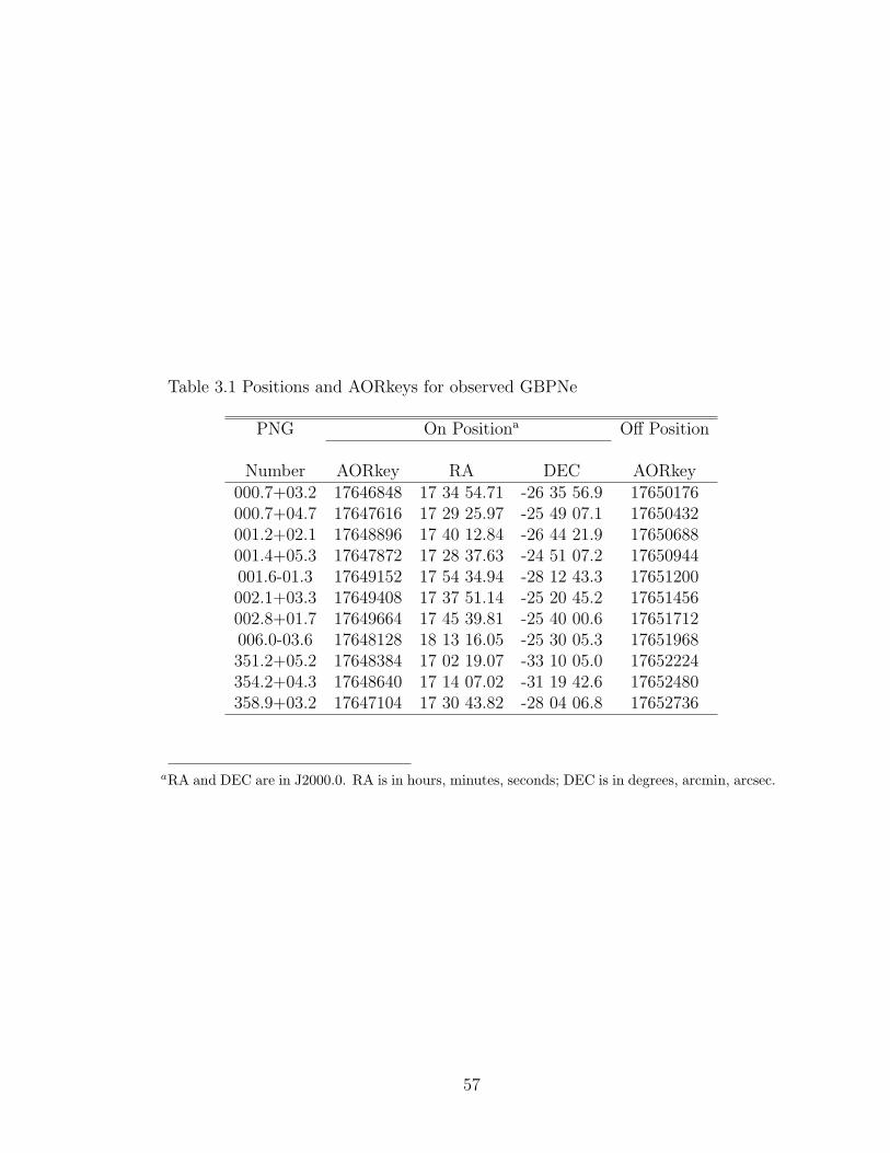
Table 3.1 Positions and AORkeys for observed GBPNe

PNG On Positiona Off Position

Number AORkey RA DEC AORkey000.7+03.2 17646848 17 34 54.71 -26 35 56.9 17650176000.7+04.7 17647616 17 29 25.97 -25 49 07.1 17650432001.2+02.1 17648896 17 40 12.84 -26 44 21.9 17650688001.4+05.3 17647872 17 28 37.63 -24 51 07.2 17650944001.6-01.3 17649152 17 54 34.94 -28 12 43.3 17651200002.1+03.3 17649408 17 37 51.14 -25 20 45.2 17651456002.8+01.7 17649664 17 45 39.81 -25 40 00.6 17651712006.0-03.6 17648128 18 13 16.05 -25 30 05.3 17651968351.2+05.2 17648384 17 02 19.07 -33 10 05.0 17652224354.2+04.3 17648640 17 14 07.02 -31 19 42.6 17652480358.9+03.2 17647104 17 30 43.82 -28 04 06.8 17652736

aRA and DEC are in J2000.0. RA is in hours, minutes, seconds; DEC is in degrees, arcmin, arcsec.

57

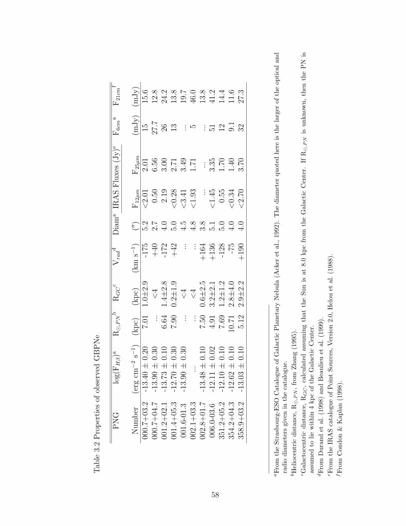
Tab

le3.

2P

roper

ties

ofob

serv

edG

BP

Ne

PN

Glo

g(F

Hβ)a

R¯,

PN

bR

GC

cV

radd

Dia

ma

IRA

SFlu

xes

(Jy)e

F6cm

aF

21cm

f

Num

ber

(erg

cm−2

s−1)

(kpc)

(kpc)

(km

s−1)

(′′ )

F12µm

F25µm

(mJy)

(mJy)

000.

7+03

.2-1

3.40±

0.20

7.01

1.0±

2.9

-175

5.2

<2.

012.

0115

15.6

000.

7+04

.7-1

3.90±

0.30

...

<4

+40

2.7

0.50

6.56

27.7

12.8

001.

2+02

.1-1

3.73±

0.10

6.64

1.4±

2.8

-172

4.0

2.19

3.00

2624

.200

1.4+

05.3

-12.

70±

0.30

7.90

0.2±

1.9

+42

5.0

<0.

282.

7113

13.8

001.

6-01

.3-1

3.90±

0.30

...

<4

...

4.5

<3.

413.

49...

19.7

002.

1+03

.3...

...

<4

...

4.8

<1.

931.

715

46.0

002.

8+01

.7-1

3.48±

0.10

7.50

0.6±

2.5

+16

43.

8...

...

...

13.8

006.

0-03

.6-1

2.11±

0.02

4.91

3.2±

2.1

+13

65.

1<

1.45

3.35

5141

.235

1.2+

05.2

-12.

10±

0.10

7.69

1.2±

1.2

-128

5.0

0.55

1.70

1214

.435

4.2+

04.3

-12.

62±

0.10

10.7

12.

8±4.

0-7

54.

0<

0.34

1.40

9.1

11.6

358.

9+03

.2-1

3.03±

0.10

5.12

2.9±

2.2

+19

04.

0<

2.70

3.70

3227

.3

aFr

omth

eSt

rasb

ourg

-ESO

Cat

alog

ueof

Gal

acti

cP

lane

tary

Neb

ula

(Ack

eret

al.,

1992

).T

hedi

amet

erqu

oted

here

isth

ela

rger

ofth

eop

tica

land

radi

odi

amet

ers

give

nin

the

cata

logu

e.bH

elio

cent

ric

dist

ance

,R¯

,PN

,fr

omZha

ng(1

995)

.cG

alac

toce

ntri

cdi

stan

ce,

RG

C,

calc

ulat

edas

sum

ing

that

the

Sun

isat

8.0

kpc

from

the

Gal

acti

cC

ente

r.If

R¯

,PN

isun

know

n,th

enth

eP

Nis

assu

med

tolie

wit

hin

4kp

cof

the

Gal

acti

cC

ente

r.dFr

omD

uran

det

al.(1

998)

and

Bea

ulie

uet

al.(1

999)

.eFr

omth

eIR

AS

cata

logu

eof

Poi

ntSo

urce

s,V

ersi

on2.

0,H

elou

etal

.(1

988)

.fFr

omC

ondo

n&

Kap

lan

(199

8).

58

3.3.3 Data Reduction

We start with basic calibrated data (bcd) from the Spitzer Science Center’s pipeline

version s15.3 or s16.1, and run it through the IRSCLEAN1 program to remove

rogue pixels, which uses a mask of rogue pixels from the same campaign as the

data. Then we take the mean of repeated observations (cycles) to improve the

signal to noise ratio. After that the background is subtracted using the off-source

positions for SH and LH, and using the off-order for SL (for example, SL1 nod1

- SL2 nod1). Next we use SMART (Higdon et al., 2004) to manually extract the

images, using full-slit extraction for SH and LH and variable-column extraction

for SL; we also inspect the spectral profiles of each target with the Manual Source

Finder tool in SMART to ensure that only one source is within the slit. Spikes due

to deviant pixels which the IRSCLEAN program missed are removed manually

in SMART. In order to account for flux that fell outside of the IRS slits (due

either to a slight mispointing and/or the extended size of the GBPNe), we apply

multiplicative scaling factors to each order and nod. The highest flux in LH sets

the scaling because LH is large enough to contain the entire flux of all of our

GBPNe. Thus, one nod in LH is scaled to the other, the SH nods are then scaled

to LH, and the SL nods and orders are then scaled to match SH. Table 3.3 gives the

scaling factors; they are usually quite small (≤1.20) except for three PNe where

the scaling factors in SL (the aperture with the smallest width) reach up to 1.70.

Figure 3.1 plots the scaled and nod-averaged spectra. We predict the 12 and 25

µm IRAS fluxes from these scaled IRS spectra and find generally good agreement

with the actual IRAS fluxes, confirming that only the IRAS source is within the

IRS slit. Finally we use the gaussian profile fitting routine in SMART to measure

line fluxes for each nod position of the scaled spectra. Table 3.4 gives the observed

1The IRSCLEAN program is available from the Spitzer Science Center’s website athttp://ssc.spitzer.caltech.edu

59

nod-averaged line fluxes. Uncertainties on the line fluxes are usually ≤10%, with

uncertainties greater than this marked in the table. A less-than sign in Table 3.4

indicates a 3σ upper limit obtained from the instrument resolution and the root

mean square (RMS) deviation in the spectrum at the wavelength of the line.

3.4 Supplementary Data

We supplement our IR data with optical and radio data from the literature to

aid abundance determinations for three reasons. First, we use the observed Hβ

and 6 cm radio fluxes to derive the extinction toward GBPNe. Table 3.2 gives

these fluxes from the Strasbourg-ESO Catalogue of Galactic Planetary Nebula

(Acker et al., 1992). Second, we adopt electron temperatures derived from ratios

of optical line fluxes (discussed in §3.5.1). Third, we use optical line fluxes for

ions not observable in our IR spectra (specifically lines fluxes of Ar IV, S II, O II,

and O III) to reduce the need for ICFs. (As an aside, no UV line data for any

of the GBPNe in our sample are available due to the large extinction toward the

Bulge.) When the optical line fluxes are given as observed line fluxes, we apply

the logarithmic extinction at Hβ (CHβ) given in the paper to correct the lines

for extinction because it gives the correct Balmer decrement. When more than

one paper gives a value for a line flux, we take the average (after correcting all

line fluxes for extinction), and Table 3.5 gives the optical extinction corrected line

fluxes adopted for the calculation of abundances.

All of the PNe in this sample should be within ∼4 kpc or less of the Galactic

Center because they were selected to be members of the Bulge. In order to de-

termine approximately where they are within the Bulge to place them on a plot

of abundance versus galactocentric distance, we adopt the heliocentric statistical

distances from Zhang (1995). We chose these distances because Zhang (1995) lists

60

distances to more of our objects than other studies, such as van de Steene & Zijl-

stra (1995) and Cahn et al. (1992). An accurate statistical distance scale for PNe

is difficult to obtain, and controversies exist as to which statistical distance scales

are the best: for example Bensby & Lundstrom (2001) find that Zhang’s distance

scale is good, while Ciardullo et al. (1999) find that it is not as good. However,

regardless of which statistical distances we adopt, the conclusions of the paper will

remain unchanged because all of the PNe in our sample are constrained to be in

the Bulge by other criteria and we include the large uncertainties that go with

these statistical distances in the data analysis.

We adopt the distance from the Sun to the Galactic Center, Ro, from Reid

(1993) who determines the best estimate of this distance by taking a weighted

average of the various determinations of Ro from different methods. Reid (1993)

finds that Ro = 8.0 ± 0.5 kpc, and this value seems to agree with more current

estimates of this distance (e.g. Lopez-Corredoira et al., 2000; Eisenhauer et al.,

2005; Groenewegen et al., 2008). Galactocentric distances (RGC) are then calcu-

lated assuming this Ro, and uncertainties on RGC are calculated using standard

error propagation and assuming an uncertainty of 40% on the heliocentric distance

(Zhang 1995 estimates the accuracy of the PN distance scale as 35-50% on aver-

age). If the distance to a PN is unknown, we assume it is within 4 kpc of the

Galactic Center. Table 3.2 lists the heliocentric and galactocentric distances for

each object.

61

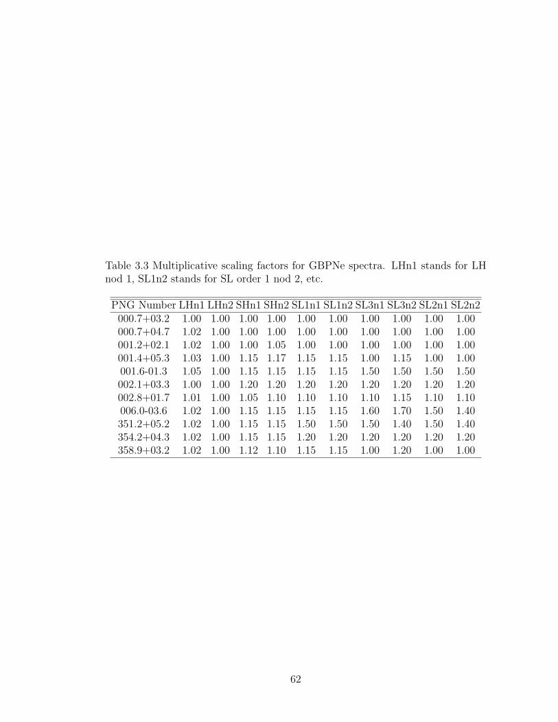
Table 3.3 Multiplicative scaling factors for GBPNe spectra. LHn1 stands for LHnod 1, SL1n2 stands for SL order 1 nod 2, etc.

PNG Number LHn1 LHn2 SHn1 SHn2 SL1n1 SL1n2 SL3n1 SL3n2 SL2n1 SL2n2000.7+03.2 1.00 1.00 1.00 1.00 1.00 1.00 1.00 1.00 1.00 1.00000.7+04.7 1.02 1.00 1.00 1.00 1.00 1.00 1.00 1.00 1.00 1.00001.2+02.1 1.02 1.00 1.00 1.05 1.00 1.00 1.00 1.00 1.00 1.00001.4+05.3 1.03 1.00 1.15 1.17 1.15 1.15 1.00 1.15 1.00 1.00001.6-01.3 1.05 1.00 1.15 1.15 1.15 1.15 1.50 1.50 1.50 1.50002.1+03.3 1.00 1.00 1.20 1.20 1.20 1.20 1.20 1.20 1.20 1.20002.8+01.7 1.01 1.00 1.05 1.10 1.10 1.10 1.10 1.15 1.10 1.10006.0-03.6 1.02 1.00 1.15 1.15 1.15 1.15 1.60 1.70 1.50 1.40351.2+05.2 1.02 1.00 1.15 1.15 1.50 1.50 1.50 1.40 1.50 1.40354.2+04.3 1.02 1.00 1.15 1.15 1.20 1.20 1.20 1.20 1.20 1.20358.9+03.2 1.02 1.00 1.12 1.10 1.15 1.15 1.00 1.20 1.00 1.00

62

Figure 3.1 Scaled, nod-averaged Spitzer IRS spectra (black) of our GBPNe. SLdata is presented below 10 µm, and HR data above 10 µm. The spline-fits to thecontinua (which we subtract from the spectra later in order to better view thecrystalline silicate features) is over-plotted (grey).

63

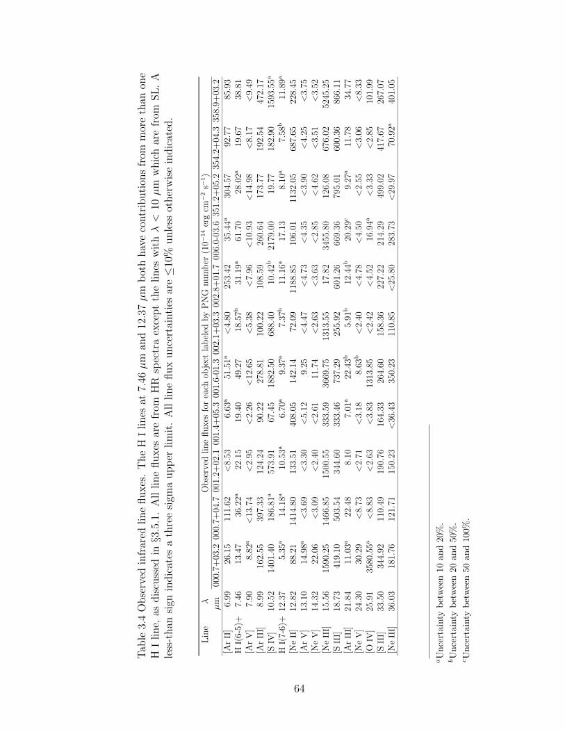
Tab

le3.

4O

bse

rved

infr

ared

line

fluxes

.T

he

HIlines

at7.

46µm

and

12.3

7µm

bot

hhav

eco

ntr

ibuti

ons

from

mor

eth

anon

eH

Iline,

asdis

cuss

edin§3

.5.1

.A

llline

fluxes

are

from

HR

spec

tra

exce

pt

the

lines

wit

hλ

<10

µm

whic

har

efr

omSL.A

less

-than

sign

indic

ates

ath

ree

sigm

aupper

lim

it.

All

line

flux

unce

rtai

nti

esar

e≤1

0%unle

ssot

her

wis

ein

dic

ated

.

Lin

eλ

Obse

rved

line

fluxes

for

each

obje

ctla

bel

edby

PN

Gnum

ber

(10−

14

erg

cm−2

s−1)

µm

000.

7+03

.200

0.7+

04.7

001.

2+02

.100

1.4+

05.3

001.

6-01

.300

2.1+

03.3

002.

8+01

.700

6.0-

03.6

351.

2+05

.235

4.2+

04.3

358.

9+03

.2[A

rII

]6.

9926

.15

111.

62<

8.53

6.63

a51

.51a

<4.

8025

3.42

35.4

4a30

4.57

92.7

785

.93

HI(

6-5)

+7.

4613

.47

36.2

2a22

.15

19.4

049

.27

18.5

7b31

.19a

61.7

028

.02a

19.6

738

.81

[Ar

V]

7.90

8.82

a<

13.7

4<

2.95

<2.

26<

12.6

5<

5.38

<7.

96<

10.9

3<

14.9

8<

8.17

<9.

49[A

rII

I]8.

9916

2.55

397.

3312

4.24

90.2

227

8.81

100.

2210

8.59

260.

6417

3.77

192.

5447

2.17

[SIV

]10

.52

1401

.40

186.

81a

573.

9167

.45

1882

.50

688.

4010

.42b

2179

.00

19.7

718

2.90

1593

.55a

HI(

7-6)

+12

.37

5.35

a14

.18a

10.5

3a6.

70a

9.37

a7.

37b

11.1

6a17

.13

8.10

a7.

58b

11.8

9a

[Ne

II]

12.8

288

.21

1414

.80

133.

5140

8.05

142.

1472

.09

1188

.85

106.

0111

32.0

568

7.65

228.

45[A

rV

]13

.10

14.9

8a<

3.69

<3.

30<

5.12

9.25

<4.

47<

4.73

<4.

35<

3.90

<4.

25<

3.75

[Ne

V]

14.3

222

.06

<3.

09<

2.40

<2.

6111

.74

<2.

63<

3.63

<2.

85<

4.62

<3.

51<

3.52

[Ne

III]

15.5

615

90.2

514

66.8

515

00.5

533

3.59

3669

.75

1313

.55

17.8

234

55.8

012

6.08

676.

0252

45.2

5[S

III]

18.7

341

9.10

503.

5434

4.60

333.

4673

7.29

255.

9260

1.26

669.

3679

5.01

600.

3686

6.11

[Ar

III]

21.8

411

.03a

22.4

88.

107.

01a

22.4

3b5.

91b

12.4

4b20

.29c

9.27

a11

.78

34.7

7[N

eV

]24

.30

30.2

9<

8.73

<2.

71<

3.18

8.63

b<

2.40

<4.

78<

4.50

<2.

55<

3.06

<8.

33[O

IV]

25.9

135

80.5

5a<

8.83

<2.

63<

3.83

1313

.85

<2.

42<

4.52

16.9

4a<

3.33

<2.

8510

1.99

[SII

I]33

.50

344.

9211

0.49

190.

7616

4.33

264.

6015

8.36

227.

2221

4.29

499.

0241

7.67

267.

07[N

eII

I]36

.03

181.

7612

1.71

150.

23<

36.4

335

0.23

110.

85<

25.8

028

3.73

<29

.97

70.9

2a40

1.05

aU

ncer

tain

tybe

twee

n10

and

20%

.bU

ncer

tain

tybe

twee

n20

and

50%

.cU

ncer

tain

tybe

twee

n50

and

100%

.

64

Tab

le3.

5E

xti

nct

ion

corr

ecte

dop

tica

lline

fluxes

.N

oop

tica

lline

fluxes

for

PN

G00

2.1+

03.3

wer

efo

und

inth

elite

ratu

re.

Ref

eren

ces:

Ack

eret

al.(1

991)

,R

atag

etal

.(1

997)

,C

uis

inie

ret

al.(2

000)

,E

scuder

oet

al.(2

004)

,an

dW

ang

&Liu

(200

7).

Lin

eλ

Exti

nct

ion

corr

ecte

dline

fluxes

rela

tive

toH

β=

100

for

each

obje

ctla

bel

edby

PN

Gnum

ber

A00

0.7+

03.2

000.

7+04

.700

1.2+

02.1

001.

4+05

.300

1.6-

01.3

002.

8+01

.700

6.0-

03.6

351.

2+05

.235

4.2+

04.3

358.

9+03

.2[O

II]

3727

114.

0...

...

...

...

...

55.1

359

.60

130.

0...

[Ne

III]

3869

69.6

...

32.8

6...

...

...

95.1

9...

9.70

...

[OII

I]43

6312

.42.

81...

...

...

...

6.68

...

...

...

[Ar

IV]+

He

I47

127.

00...

...

...

...

...

1.91

...

...

...

[Ar

IV]

4740

4.61

...

...

...

...

...

1.93

...

...

...

[OII

I]49

5927

9.1

123.

9923

1.9

118.

235

4.2

...

369.

547.

2746

.41

339.

1[O

III]

5007

790.

436

0.37

728.

030

4.7

1003

.822

.65

1067

.55

25.8

913

6.5

989.

4[S

III]

6312

1.86

1.37

1.34

0.71

...

...

2.08

...

1.01

2.02

[SII

]67

1713

.35

2.76

2.77

2.70

6.40

4.77

4.35

6.46

5.96

6.68

[SII

]67

3119

.47

5.12

4.37

3.30

14.3

89.

067.

839.

319.

3612

.41

[Ar

V]

7005

0.67

...

...

...

...

...

...

...

...

...

[Ar

III]

7135

30.7

929

.22

15.7

912

.24

21.5

46.

5616

.15

4.86

9.34

30.6

6[A

rIV

]72

36...

0.96

...

...

...

...

...

...

...

...

[Ar

IV]

7264

...

1.06

...

...

...

...

...

...

...

...

[OII

]73

255.

1511

.42

7.10

8.33

...

3.87

6.29

0.91

2.07

7.73

65

3.5 Data Analysis

3.5.1 Abundances

Before determining abundances for this sample of GBPNe, we must first calcu-

late and then correct for extinction. Additionally we adopt electron temperatures

(Te) from the literature and then employ infrared line ratios to derive the electron

densities (Ne). After that we use the values of the above quantities to obtain abun-

dances for each ion. The following subsection discuss the details of the calculations

of extinction, the selection of Te and Ne, and finally the derivation of ionic and

total abundances.

Extinction Correction

We first calculate the reddening correction by comparing the Hβ flux predicted

from IR hydrogen recombination lines to the observed Hβ flux (see Table 3.6). In

order to predict the Hβ flux from the IR H I lines, we adopt the theoretical ratios

of hydrogen recombination lines from Hummer & Storey (1987) and assume case

B recombination for a gas at Te= 104 K and Ne= 103 cm−3. The H I(7-6) line

at 12.37 µm and the H I(11-8) line at 12.39 µm are blended in the SH spectrum,

and theoretically the H I(7-6) line contributes 89% of total line flux. Similarly,

nearby lines of H I(6-5), H I(17-8), H I(8-6), and H I(11-7) contribute to the H I

line at 7.46 µm, with the H I(6-5) flux theoretically contributing 74% of the total

line flux. The contributions of additional lines are removed before calculating the

predicted Hβ flux from the H I(7-6) and H I(6-5) IR lines.

Additionally we calculate extinction by comparing the Hβ flux predicted from

the radio flux at 6cm to the observed Hβ flux. We assume that Te=104 K (and

thus t ≡ Te/104 K = 1), He+/H+=0.09, and He++/H+=0.03 and use the following

66

formula from Pottasch (1984):

F (Hβ)predicted6cm =

S6cm

2.82× 109t0.53(1 + He+/H+ + 3.7He++/H+)

where 2.82×109 converts units so that S6cm is in Jy and F(Hβ) is in erg cm−2 s−1.

Table 3.2 gives the values for S6cm and F(Hβ) while Table 3.6 gives the calculated

values of the extinction.

For the abundance calculations, in order to weight the extinctions calculated

from both of the above methods equally, we use

CHβ,final =CHβ,HI(7−6)

4+

CHβ,HI(6−5)

4+

CHβ,radio

2

when we have extinctions from both H I lines and the radio, otherwise we just take

an average (see Table 3.8 for these adopted values). There is no Hβ flux available

for PNG002.1+03.3 and thus we adopt an extinction to it from the average of the

other GBPNe extinctions. Table 3.6 gives the extinction values derived here along

with those from the literature. In general there is very good agreement between

the different methods.

We use the extinction law from Fluks et al. (1994) and assume the standard

RV of the Milky Way of 3.1. However, there is evidence that interstellar extinction

is steeper than this toward the Bulge, e.g. Walton et al. (1993b) find that RV =2.3

and Ruffle et al. (2004) find RV = 2.0. Nevertheless, abundances determined from

IR lines are not greatly affected by this change in RV : an RV =2.0 usually changes

their abundances by .5% (and at most 10%) compared to the usual RV =3.1.

Thus, because the previous optical studies to which we compare assumed RV =3.1,

and because the IR lines are even less affected by the choice of RV , we assume

RV =3.1.

67

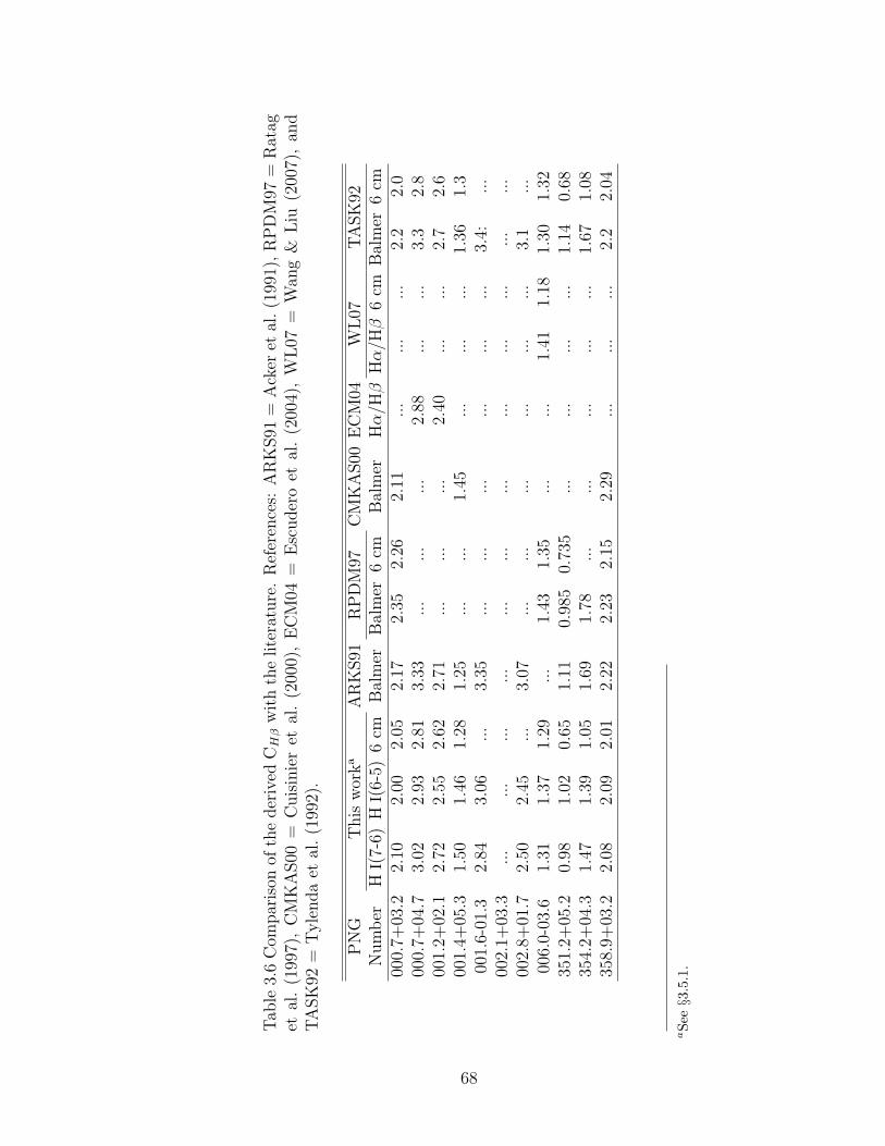
Tab

le3.

6C

ompar

ison

ofth

eder

ived

CH

βw

ith

the

lite

ratu

re.

Ref

eren

ces:

AR

KS91

=A

cker

etal

.(1

991)

,R

PD

M97

=R

atag

etal

.(1

997)

,C

MK

AS00

=C

uis

inie

ret

al.

(200

0),

EC

M04

=E

scuder

oet

al.

(200

4),

WL07

=W

ang

&Liu

(200

7),

and

TA

SK

92=

Tyle

nda

etal

.(1

992)

.

PN

GT

his

wor

ka

AR

KS91

RP

DM

97C

MK

AS00

EC

M04

WL07

TA

SK

92N

um

ber

HI(

7-6)

HI(

6-5)

6cm

Bal

mer

Bal

mer

6cm

Bal

mer

Hα/H

βH

α/H

β6

cmB

alm

er6

cm00

0.7+

03.2

2.10

2.00

2.05

2.17

2.35

2.26

2.11

...

...

...

2.2

2.0

000.

7+04

.73.

022.

932.

813.

33...

...

...

2.88

...

...

3.3

2.8

001.

2+02

.12.

722.

552.

622.

71...

...

...

2.40

...

...

2.7

2.6

001.

4+05

.31.

501.

461.

281.

25...

...

1.45

...

...

...

1.36

1.3

001.

6-01

.32.

843.

06...

3.35

...

...

...

...

...

...

3.4:

...

002.

1+03

.3...

...

...

...

...

...

...

...

...

...

...

...

002.

8+01

.72.

502.

45...

3.07

...

...

...

...

...

...

3.1

...

006.

0-03

.61.

311.

371.

29...

1.43

1.35

...

...

1.41

1.18

1.30

1.32

351.

2+05

.20.

981.

020.

651.

110.

985

0.73

5...

...

...

...

1.14

0.68

354.

2+04

.31.

471.

391.

051.

691.

78...

...

...

...

...

1.67

1.08

358.

9+03

.22.

082.

092.

012.

222.

232.

152.

29...

...

...

2.2

2.04

aSe

e§3

.5.1

.

68

Electron Temperature and Density

In order to derive abundances, we adopt two electron temperatures (Te): T[N II]

for the low-ionization potential ions (Ar II, Ne II, S II, and O II), and T[O III] for

the high-ionization potential ions. Table 3.7 gives the electron temperatures from

the literature. When possible, our adopted T[N II] and T[O III] are an average of

the values from the literature. If temperatures are not available in the literature, we

assume the average value from the other GBPNe in the sample (<T[N II]> = 8100

K and <T[O III]> = 10700 K). Abundances from IR lines depend only weakly on

the adopted Te, and thus our assumption does not strongly affect our abundances

— especially those of argon, neon, and sulfur which are mostly determined from

IR lines.

We determine electron densities (Ne) from IR line ratios of S III, Ne III, Ar III,

Ar V, and Ne V (see Table 3.7). The S III line ratio gives the best estimate of

Ne, and thus we adopt it for the abundance analysis. Densities determined from

the other line ratios are more uncertain because they either rely on at least one

line with a weak flux, or the density is outside the range of what the line ratio can

accurately measure. The adopted Ne from the S III ratios have an average of 3500

cm−3, and range from 1000 to 9200 cm−3.

Ionic and Total Abundances

Table 3.8 lists the parameters used in determining the PNe ionic abundances. Note

that we use a predicted Hβ flux from the IR H I lines in order to ensure that the

hydrogen comes from within the same slit as the IR forbidden lines. Table 3.9

presents the ionic abundances themselves. In order to determine total elemental

abundances, the ionic abundances for each element are summed. When the ionic

abundance can be determined by more than one line, we choose the abundance(s)

69

from the most reliable line(s), and mark the lines used in Table 3.9. If necessary, the

sum of the ionic abundances for each element is then multiplied by an ionization

correction factor (ICF) to account for unobserved ions that are expected to be

present. For argon, we apply an ICF for the nine objects for which Ar+3 is not

observed. For neon, we apply an ICF for the four high ionization nebulae with

unobserved Ne+3. ICFs are generally small, and we can derive accurate total

elemental abundances for many objects, especially for the elements of neon and

sulfur whose abundances are derived mainly from IR lines and which rarely need

ICFs. Table 3.10 presents the total elemental abundances.

The Ar+3 abundance can only be determined directly from optical lines for

two of the GBPNe (PNG000.7+03.2 and PNG006.0-03.6). However, the Ar+3

abundance cannot contribute a large amount because the abundance of Ar+4 always

accounts for <2% of the total argon abundance. We adopt an ICF to account for

unobserved Ar+3 determined by Ar+3 = 0.28*Ar+2 because the two GBPNe with

observed Ar+3 have Ar+3/Ar+2 = 0.27 and 0.29. Additionally, the GDPNe in the

sample of Pottasch & Bernard-Salas (2006) for which the ionic abundance of Ar+4

is less than 2% of the total argon abundance (like our sample of GBPNe) have

Ar+3/Ar+2 ranging from 0.15 to 0.68 with a mean of 0.30, so our assumption of

Ar+3 = 0.28*Ar+2 is justified.

The Ne+3 abundance cannot be determined directly for any of our GBPNe

because its lines lie in the UV. However, it is only expected to contribute sig-

nificantly if the O+3 line is detected in the IRS spectrum because its ionization

potential (IP=63.45 eV) is near that of O+3 (IP = 54.93 eV). The O+3 line is de-

tected in only four of the spectra of our GBPNe (PNG000.7+03.2, PNG001.6-01.3,

PNG006.0-03.6, and PNG358.9+03.2). Thus, for these four objects only, an ICF

is necessary to account for unobserved Ne+3. Similarly to Ar+3, the Ne+3 cannot

70

contribute a huge amount because the abundance of Ne+4 always accounts for <1%

of the total abundance of neon. Taking the average of a sample of Galactic PNe,

Bernard-Salas et al. (2008) find that Ne+3 = 0.35*(Ne+2 + Ne+4), and thus we

adopt an ICF determined by this to account for unobserved Ne+3.

The uncertainties in the derived elemental abundances result from uncertainties

in the line fluxes, CHβ, Te, Ne and ICFs. The measured H I line fluxes typically

have uncertainties .20%, while the measured fine structure line fluxes usually

have uncertainties .10%. Uncertainties are also introduced into the line fluxes

from the adopted scaling factors which are typically .15% for the high resolution

lines (those lines above 10 µm), but reach 50–70% for the low resolution lines for

three objects. However, our scaling factors cannot be far off because the CHβ

determined from H I lines in in the high and low resolution spectra agree well

and the ionic Ar+2 abundance determined from Ar III lines in the high and low

resolution spectra also agree well, even for the nebulae with the largest scaling

factors. The uncertainties in CHβ and Te of ∼10% each do not have a large

affect on the total elemental abundances of argon, neon, and sulfur because these

abundances are determined mainly from IR lines; however, they will have a larger

affect on the total abundance of oxygen. The uncertainty on Ne is ∼30%. The

uncertainties on the ICFs for argon and neon are most likely less than a factor of

two, causing an abundance uncertainty for these elements of .30% due to the ICFs

(when the ICFs are neccessary). A comparison to optically derived abundances for

the same objects by various authors gives an estimate of the typical total abundance

uncertainty of ∼50% (this work, Gorny et al., 2004; Bernard-Salas et al., 2008).

71

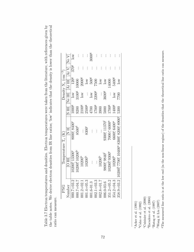
Tab

le3.

7E

lect

ron

tem

per

ature

san

dden

siti

es.

Ele

ctro

nte

mper

ature

sw

ere

take

nfr

omth

elite

ratu

re,w

ith

refe

rence

sgi

ven

by

the

table

not

es.

We

der

ive

elec

tron

den

siti

esfr

omIR

line

rati

os;‘low

’in

dic

ates

that

the

den

sity

islo

wer

than

the

theo

reti

cal

rati

oca

nm

easu

re.

PN

GTem

per

ature

Te

(K)

Den

sity

Ne

(cm−3

)N

um

ber

[OII

I][N

II]

[SII

I][N

eII

I][A

rII

I][A

rV

][N

eV

]00

0.7+

03.2

1020

0b ,13

300e

8000

c ,84

00e

1000

glo

w12

0g37

0glo

w00

0.7+

04.7

1020

0d ,10

200b

8500

d92

0031

00g

1000

0...

...

001.

2+02

.110

200b

...

2100

glo

w20

00g

...

...

001.

4+05

.310

200b

8300

c25

00g

...

low

...

...

001.

6-01

.3...

...

4700

low

500g

...

3000

g

002.

1+03

.3...

...

1700

g22

00g

7500

...

...

002.

8+01

.710

200b

...

3900

...

low

...

...

006.

0-03

.698

00e ,98

40f

9300

e ,11

370f

5000

3600

glo

w...

...

351.

2+05

.210

200b ,

9300

e70

00:e ,

6000

a17

00g

...

1400

0...

...

354.

2+04

.310

200b

6600

e ,64

00a

1400

glo

w54

00g

...

...

358.

9+03

.210

200b ,

7700

e ,10

400a

8300

e ,82

00a ,89

00c

5300

7700

low

...

...

aA

cker

etal

.(1

991)

bC

ahn

etal

.(1

992)

cC

uisi

nier

etal

.(2

000)

dE

scud

ero

etal

.(2

004)

eR

atag

etal

.(1

997)

fW

ang

&Liu

(200

7)gT

hem

easu

red

line

rati

ois

atth

elo

wen

d(i

nth

eno

n-lin

ear

regi

me)

ofth

ede

nsit

ies

that

the

theo

reti

callin

era

tio

can

mea

sure

.

72

Table 3.8 Adopted parameters for determining abundances

PNG FHβ ,predicted CHβNe T[O III] T[N II]

Number (10−14 erg cm−2 s−1) (cm−3) (K) (K)000.7+03.2 483 2.05 1000 11800 8200000.7+04.7 1328 2.89 9200 10200 8500001.2+02.1 902 2.62 2100 10200 8100b

001.4+05.3 630 1.38 2500 10200 8300001.6-01.3 1280 2.95 4700 10700b 8100b

002.1+03.3 662a 1.87a 1700 10700b 8100b

002.8+01.7 1071 2.47 3900 10200 8100b

006.0-03.6 1791 1.32 5000 9800 10300351.2+05.2 816 0.82 1700 9800 6500354.2+04.3 674 1.23 1400 10200 6500358.9+03.2 1211 2.04 5300 14200 8500

aNo extinction nor Hβ flux is given in literature for PNG002.1+03.3, so we cannot calculate theextinction from our data. We use the average extinction of the other GBPNe (CHβ= 1.87) forthe extinction toward PNG002.1+03.3.

bWhen we could not find T[O III] or T[N II] in the literature, we adopted the average value fromthe other GBPNe in this sample.

73

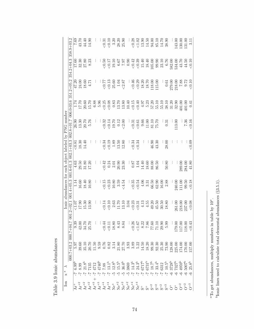
Tab

le3.

9Io

nic

abundan

ces

Ion

xa

λIo

nic

abundan

ces

for

each

obje

ctla

bel

edby

PN

Gnum

ber

000.

7+03

.200

0.7+

04.7

001.

2+02

.100

1.4+

05.3

001.

6-01

.300

2.1+

03.3

002.

8+01

.700

6.0-

03.6

351.

2+05

.235

4.2+

04.3

358.

9+03

.2A

r+-7

6.99

b5.

979.

39<

1.07

1.14

4.63

<0.

8126

.90

1.74

47.2

017

.60

7.69

Ar+

2-7

8.99

39.6

042

.00

17.9

016

.60

29.5

018

.30

13.3

017

.70

24.0

032

.30

43.7

0A

r+2

-721

.8b

35.1

034

.70

15.3

018

.40

31.8

014

.40

20.7

020

.60

18.6

027

.80

44.4

0A

r+2

-771

3520

.70

25.7

013

.90

10.8

017

.20

...

5.76

15.7

04.

718.

2314

.90

Ar+

3+

-747

1211

.50

...

...

...

...

...

...

6.88

...

...

...

Ar+

3-7

4740

b9.

59...

...

...

...

...

...

5.96

...

...

...

Ar+

4-7

7.88

0.76

<0.

44<

0.14

<0.

15<

0.42

<0.

34<

0.32

<0.

25<

0.77

<0.

50<

0.31

Ar+

4-7

13.1

b0.

82<

0.11

<0.

10<

0.23

0.24

<0.

19<

0.14

<0.

08<

0.13

<0.

17<

0.10

Ne+

-512

.8b

3.14

18.8

02.

6310

.80

2.01

1.89

19.7

00.

8325

.60

19.1

03.

20N

e+2

-515

.5b

21.8

08.

4311

.70

3.59

20.9

013

.50

0.12

13.7

01.

046.

6728

.20

Ne+

2-5

36.0

b27

.70

8.84

13.1

0<

4.54

23.3

012

.80

<2.

0013

.80

<2.

877.

9725

.90

Ne+

2-5

3869

3.93

...

3.04

...

...

...

...

10.4

0...

0.90

...

Ne+

4-7

14.3

b3.

89<

0.26

<0.

23<

0.35

0.87

<0.

34<

0.31

<0.

15<

0.46

<0.

42<

0.28

Ne+

4-7

24.3

b5.

22<

1.67

<0.

31<

0.54

1.04

<0.

34<

0.61

<0.

40<

0.29

<0.

39<

1.02

S+

-767

17b

14.5

08.

224.

134.

0614

.40

...

9.66

4.97

18.2

015

.40

13.9

0S

+-7

6731

b18

.20

7.86

4.55

3.31

18.6

0...

11.0

05.

2318

.70

18.4

014

.50

S+

2-7

18.7

b99

.30

77.6

049

.20

66.5

088

.00

46.9

081

.10

57.2

011

8.00

105.

0094

.00

S+

2-7

33.4

b92

.30

71.1

045

.50

62.9

086

.50

43.3

075

.70

55.1

011

5.00

99.9

085

.10

S+

2-7

6312

25.3

029

.90

30.5

016

.00

...

...

...

55.1

0...

23.1

014

.70

S+

3-7

10.5

b73

.90

5.99

18.8

02.

8850

.80

28.0

00.

3138

.10

0.61

6.76

38.9

0O

+-6

3728

b12

8.00

...

...

...

...

...

...

31.2

027

9.00

582.

00...

O+

-673

27b

225.

0017

9.00

261.

0024

0.00

...

...

113.

0032

.90

218.

0053

4.00

143.

00O

+2

-649

59b

174.

0011

7.00

218.

0011

1.00

289.

00...

...

401.

007.

8843

.70

130.

00O

+2

-650

07b

170.

0011

8.00

237.

0099

.50

284.

00...

7.36

401.

009.

7244

.50

131.

00O

+3

-625

.8b

157.

00<

0.43

<0.

08<

0.18

41.8

0<

0.09

<0.

160.

41<

0.10

<0.

103.

11

aTo

get

abun

danc

es,m

ulti

ply

num

bers

inta

ble

by10

x.

bIo

nic

lines

used

toca

lcul

ate

tota

lel

emen

talab

unda

nces

(§3.5

.1).

74

Tab

le3.

10C

ompar

ison

ofto

talel

emen

talab

undan

ces

for

indiv

idual

Bulg

eP

Ne.

Obta

inab

undan

ces

rela

tive

tohydro

gen

by

mult

iply

ing

the

num

ber

sin

the

Tab

leby

10x

wher

ex

is-6

for

argo

n,-4

for

neo

n,-5

for

sulfur,

and

-4fo

rox

yge

n.

PN

GT

his

wor

kR

PD

M97

aC

MK

AS00

bE

CM

04c

WL07

d

Num

ber

Ar

Ne

SO

Ar

Ne

SO

Ar

SO

Ar

Ne

SO

Ar

Ne

SO

000.

7+03

.25.

23.

71.

95.

14.

80.

560.

622.

17.

12.

010

.0...

...

...

...

...

...

...

...

000.

7+04

.75.

42.

70.

883.

0...

...

...

...

...

...

...

4.4

...

0.36

1.9

...

...

...

...

001.

2+02

.12.

01.

50.

704.

9...

...

...

...

...

...

...

1.7

0.35

0.46

3.0

...

...

...

...

001.

4+05

.32.

51.

40.

713.

5...

...

...

...

1.9:

0.56

4.9

...

...

...

...

...

...

...

...

001.

6–01

.34.

63.

21.

63.

3...

...

...

...

...

...

...

...

...

...

...

...

...

...

...

002.

1+03

.31.

81.

50.

73...

...

...

...

...

...

...

...

...

...

...

...

...

...

...

...

002.

8+01

.75.

32.

00.

891.

2...

...

...

...

...

...

...

...

...

...

...

...

...

...

...

006.

0–03

.62.

81.

90.

994.

32.

31.

10.

854.

8...

...

...

...

...

...

...

1.9

0.98

1.3

4.6

351.

2+05

.27.

12.

71.

42.

62.

9...

2.3

2.2

...

...

...

...

...

...

...

...

...

...

...

354.

2+04

.35.

32.

61.

36.

03.

81.

60.

717.

2...

...

...

...

...

...

...

...

...

...

...

358.

9+03

.26.

54.

01.

42.

85.

65.

10.

369.

33.

6:1.

26.

3...

...

...

...

...

...

...

...

aR

atag

etal

.(1

997)

.bC

uisi

nier

etal

.(2

000)

.T

heco

lon

(:)

deno

tes

low

qual

ity

abun

danc

esdu

eto

ala

ckof

data

.cE

scud

ero

etal

.(2

004)

.dW

ang

&Liu

(200

7).

75

3.5.2 Crystalline Silicates

Crystalline silicate features are present around 28 and 33 µm in the spectra of

all GBPNe in our sample, while no amorphous silicate features are observed. In

order to illustrate the crystalline silicate features more clearly, we define and sub-

tract a continuum determined by a smooth spline fit to feature-free regions of each

spectrum. Figure 3.1 shows the spline fit to the spectral continua and Figure 3.2

shows the continuum-subtracted spectra. The spline fit continuum is physically

meaningless, and we only use it to elucidate the crystalline silicate features. Fol-

lowing Molster (2000) we identify the 28 micron complex (26.5 – 31.5 µm) and 33

micron complex (31.5 µm to past the end of our spectra) both as having features

originating from the magnesium-rich crystalline silicates forsterite (Mg2SiO4) and

enstatite (MgSiO3).

The strength of the silicate emission bands can give an approximate estimate

of the crystalline dust temperatures. Matsuura et al. (2004) note that the absence

of a 23.7 µm feature indicates that forsterite is cooler than 100 K. This feature

is either not present or very weak in the spectra of our GBPNe, and thus the

forsterite dust in these objects must be cold, with a temperature .100 K.

3.5.3 PAHs

PAHs are present in six of the eleven GBPNe in our sample: PNG000.7+04.7,

PNG002.8+01.7, PNG006.0-03.6, PNG351.2+05.2, PNG354.2+04.3, and

PNG358.9+03.2. Absorption of energetic photons excites the PAH emission

features at 6.2, 7.7, 8.6, 11.2, and 12.7 µm. PAHs which emit in this spectral

range have on the order of tens to hundreds of carbon atoms (Schutte et al., 1993).

C—C stretching and bending or deformations causes the 6.2 and 7.7 µm features,

while in-plane C—H bending produces the 8.6 µm feature, and out-of-plane C—H

76

bending gives rise to the 11.2 and 12.7 µm features (Allamandola et al., 1989).

Table 3.11 gives the net integrated PAH fluxes. We calculate these by first

subtracting a spline-fit continuum and then summing the remaining flux in each

PAH wavelength range; if atomic lines are present, we subsequently subtract their

flux to arrive at the net PAH flux. For the 7.7 µm PAH, we subtract the H I

line at 7.46 µm (and for PNG006.0-03.6 and PNG358.9+03.2 the 7.32 µm line as

well). For the 12.7 µm PAH, we remove the contribution from the Ne+ line at

12.81 µm; however, the 12.7 µm PAH is much weaker than the 12.81 µm Ne+ line,

and thus the net 12.7 µm PAH flux is very uncertain. The 11.29 µm H I is weak

and always near the 3-σ upper limit in our spectra; it contributes less than 5% to

the 11.2 µm PAH flux (except for PNG006.0-03.6 and PNG358.9+03.2 where it

may contribute up to 20%) and we do not remove it. Figure 3.3 shows plots of the

continuum-subtracted, normalized PAH profiles.

3.6 Discussion

3.6.1 Elemental Abundances

Comparison of Abundances of Individual Objects with the Literature

In Table 3.10 we compare total elemental abundances from this work with abun-

dances from four papers in the literature: Ratag et al. (1997); Cuisinier et al.

(2000); Escudero et al. (2004); Wang & Liu (2007). All of these studies derive

total elemental abundances from collisionally excited optical lines, and therefore

their abundances are more dependent on the adopted extinction and electron tem-

perature than the current study. A detailed comparison with these studies is

hindered by the fact that only one study (Wang & Liu, 2007) lists their ionic

abundances and ICFs. For individual objects, our total elemental abundances of

77

argon, neon, and sulfur tend to be higher than the optical abundances. This is

due in part to the fact that the IR derived abundances for ions of Ar+2, Ne+2 and

S+2 always give a higher ionic abundance than the optically derived abundances

for the same ions. On the other hand, the total elemental abundances of oxygen

derived here do not have such a systematic offset because the main contributors to

the total oxygen abundance, O+ and O+2, are determined from optical line fluxes

which are taken from the same literature sources to which we compare abundances;

PNG002.1+03.3 does not have an oxygen abundance listed in Table 3.10 because

we could not find any optical line fluxes for this object.

Argon The values for the total argon abundance in this work are systematically

higher than the values given in the literature (except in one case where the values

are close). Several factors can lead to this offset: (1) In most cases, total elemental

argon abundances in this work and prior studies of the GBPNe in our sample must

use an ICF to account for unobserved Ar+3; different ICFs will lead to different

total argon abundances. When the 4740 A Ar+3 line is observed, our elemental

argon abundance value agrees to within 30% of the values in the literature. (2) For

the low excitation PNe (PNG002.8+01.7, PNG351.2+05.2, and PNG354.2+04.3,

Excitation Class, EC∼2–3), the IR data show that Ar+ contributes significantly

to the total argon abundance, and thus optical studies without observed Ar+ must

either use an ICF to account for it or risk underestimating the total argon abun-

dance. (3) When we derive the Ar+2 ionic abundance from the IR lines and the

optical 7135 A line, we always get a value from the IR lines that is higher than that

from the optical line (often within 50%, but sometimes off by a factor of a few),

which causes many of our IR derived total argon abundances to be systematically

higher than those derived in the literature. This may be due to the uncertainty in

Te when using optical lines to derive the Ar+2 abundance: lowering the electron

78

temperature by 1000 to 2000 K significantly increases the Ar+2 ionic abundance

derived from the optical line (while only slightly increasing the Ar+2 ionic abun-

dance derived from the IR lines), bringing the optical Ar+2 abundances into good

agreement with the IR Ar+2 abundances in most cases.

Neon The values for the total neon abundance are systematically higher in

this study than in the literature (in all except one case where the values are close).

The factors that may cause this are: (1) The IR data show that Ne+ is the

dominant contributor to the total elemental neon abundance in roughly half of

our GBPNe. There is no Ne+ line observable in the optical, and thus the optical

studies have not observed the most important ionization stage of neon for these

PNe. (2) Lines of Ne+3 lie in the UV part of the spectrum, and thus our study

and previous optical studies must use an ICF to account for it in high ionization

nebulae (PNG000.7+03.2, PNG001.6-01.3, PNG006.0-03.6, and PNG358.9+03.2);

different assumed ICFs could account for part of the discrepancy for these PNe. (3)

When we derive the Ne+2 ionic abundance from the IR lines and the optical 3869

A line, we always get a value from the IR lines that is higher than that from the

optical. Similarly to Ar+2, this may be due (at least in part) to the uncertainty in

Te having large affects on the optically derived abundances. Lowering the electron

temperature by 1000 to 2000 K increases the Ne+2 ionic abundance derived from

the optical line (while only slightly changing the Ne+2 ionic abundance derived

from the IR lines), bringing the optical and IR derived Ne+2 abundances into

better agreement.

79

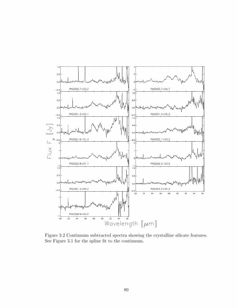
Figure 3.2 Continuum subtracted spectra showing the crystalline silicate features.See Figure 3.1 for the spline fit to the continuum.

80

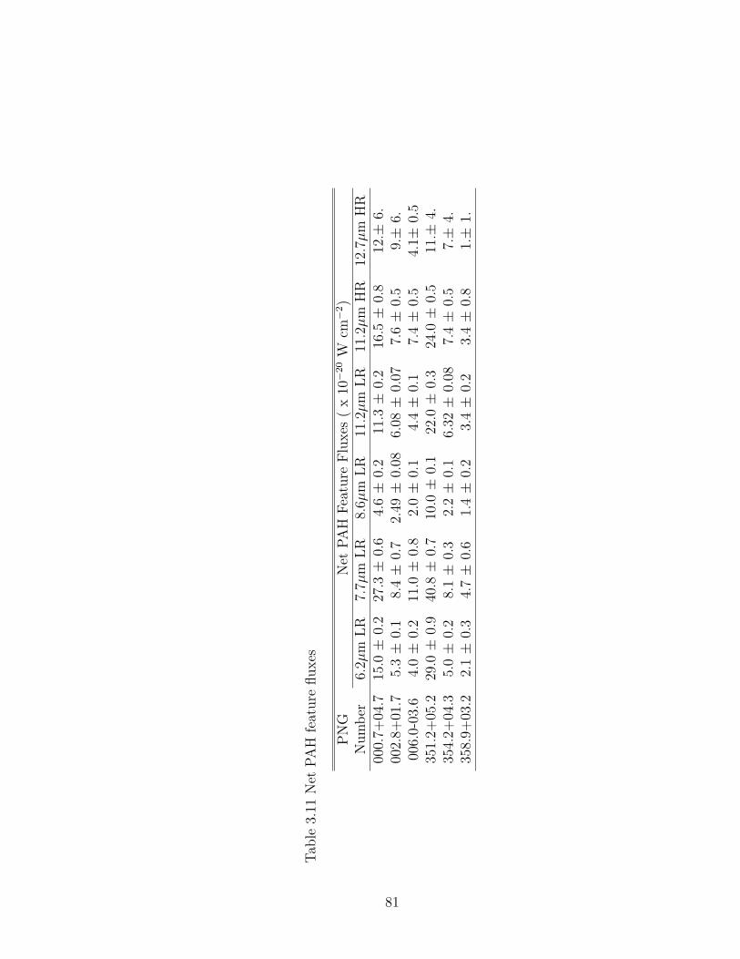
Tab

le3.

11N

etPA

Hfe

ature

fluxes

PN

GN

etPA

HFea

ture

Flu

xes

(x

10−2

0W

cm−2

)N

um

ber

6.2µ

mLR

7.7µ

mLR

8.6µ

mLR

11.2

µm

LR

11.2

µm

HR

12.7

µm

HR

000.

7+04

.715

.0±

0.2

27.3±

0.6

4.6±

0.2

11.3±

0.2

16.5±

0.8

12.±

6.00

2.8+

01.7

5.3±

0.1

8.4±

0.7

2.49±

0.08

6.08±

0.07

7.6±

0.5

9.±

6.00

6.0-

03.6

4.0±

0.2

11.0±

0.8

2.0±

0.1

4.4±

0.1

7.4±

0.5

4.1±

0.5

351.

2+05

.229

.0±

0.9

40.8±

0.7

10.0±

0.1

22.0±

0.3

24.0±

0.5

11.±

4.35

4.2+

04.3

5.0±

0.2

8.1±

0.3

2.2±

0.1

6.32±

0.08

7.4±

0.5

7.±

4.35

8.9+

03.2

2.1±

0.3

4.7±

0.6

1.4±

0.2

3.4±

0.2

3.4±

0.8

1.±

1.

81

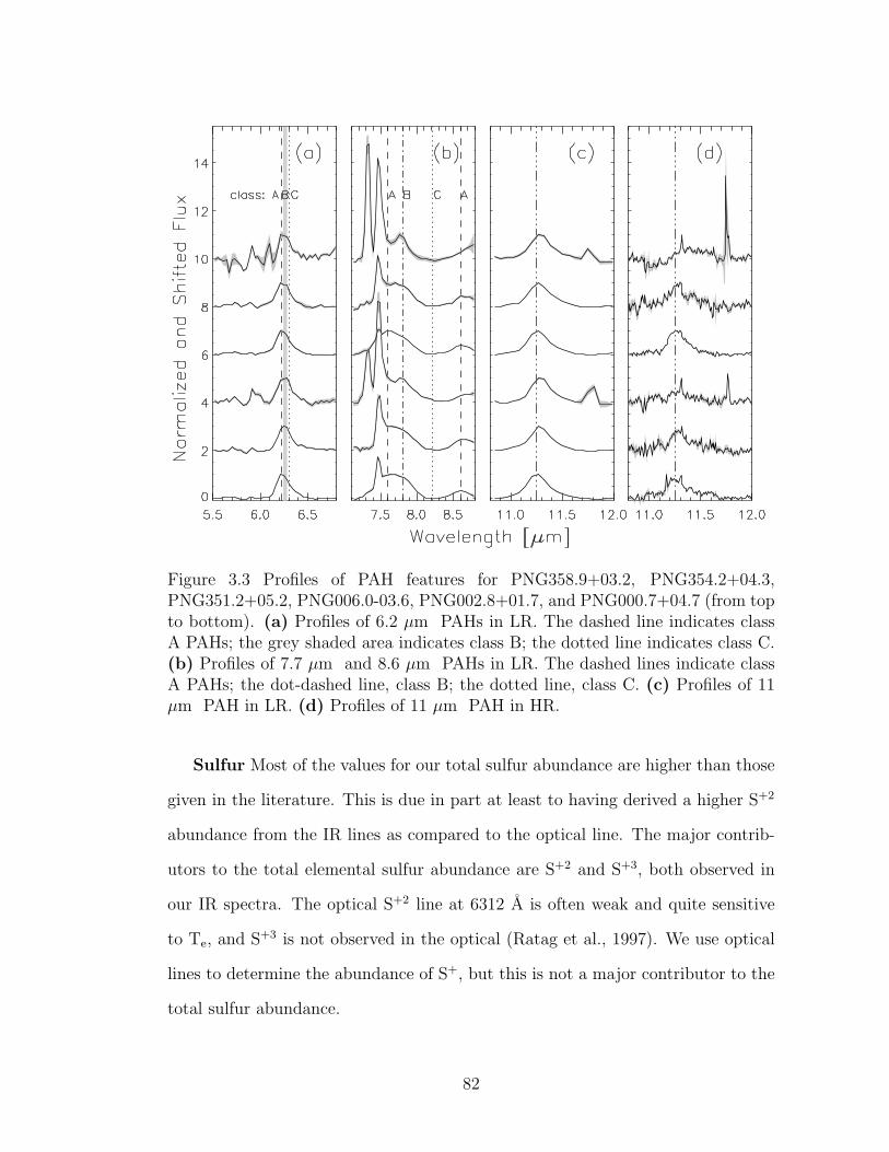
Figure 3.3 Profiles of PAH features for PNG358.9+03.2, PNG354.2+04.3,PNG351.2+05.2, PNG006.0-03.6, PNG002.8+01.7, and PNG000.7+04.7 (from topto bottom). (a) Profiles of 6.2 µm PAHs in LR. The dashed line indicates classA PAHs; the grey shaded area indicates class B; the dotted line indicates class C.(b) Profiles of 7.7 µm and 8.6 µm PAHs in LR. The dashed lines indicate classA PAHs; the dot-dashed line, class B; the dotted line, class C. (c) Profiles of 11µm PAH in LR. (d) Profiles of 11 µm PAH in HR.

Sulfur Most of the values for our total sulfur abundance are higher than those

given in the literature. This is due in part at least to having derived a higher S+2

abundance from the IR lines as compared to the optical line. The major contrib-

utors to the total elemental sulfur abundance are S+2 and S+3, both observed in

our IR spectra. The optical S+2 line at 6312 A is often weak and quite sensitive

to Te, and S+3 is not observed in the optical (Ratag et al., 1997). We use optical

lines to determine the abundance of S+, but this is not a major contributor to the

total sulfur abundance.

82

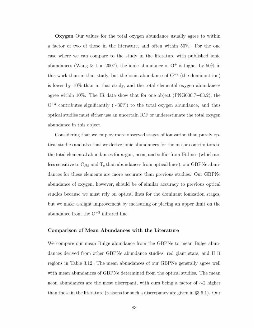
Oxygen Our values for the total oxygen abundance usually agree to within

a factor of two of those in the literature, and often within 50%. For the one

case where we can compare to the study in the literature with published ionic

abundances (Wang & Liu, 2007), the ionic abundance of O+ is higher by 50% in

this work than in that study, but the ionic abundance of O+2 (the dominant ion)

is lower by 10% than in that study, and the total elemental oxygen abundances

agree within 10%. The IR data show that for one object (PNG000.7+03.2), the

O+3 contributes significantly (∼30%) to the total oxygen abundance, and thus

optical studies must either use an uncertain ICF or underestimate the total oxygen

abundance in this object.

Considering that we employ more observed stages of ionization than purely op-

tical studies and also that we derive ionic abundances for the major contributors to

the total elemental abundances for argon, neon, and sulfur from IR lines (which are

less sensitive to CHβ and Te than abundances from optical lines), our GBPNe abun-

dances for these elements are more accurate than previous studies. Our GBPNe

abundance of oxygen, however, should be of similar accuracy to previous optical

studies because we must rely on optical lines for the dominant ionization stages,

but we make a slight improvement by measuring or placing an upper limit on the

abundance from the O+3 infrared line.

Comparison of Mean Abundances with the Literature

We compare our mean Bulge abundance from the GBPNe to mean Bulge abun-

dances derived from other GBPNe abundance studies, red giant stars, and H II

regions in Table 3.12. The mean abundances of our GBPNe generally agree well

with mean abundances of GBPNe determined from the optical studies. The mean

neon abundances are the most discrepant, with ours being a factor of ∼2 higher

than those in the literature (reasons for such a discrepancy are given in §3.6.1). Our

83

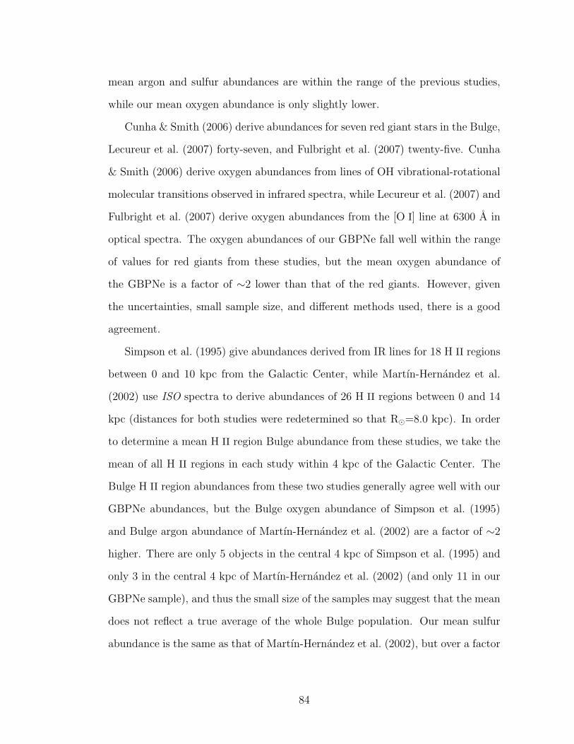
mean argon and sulfur abundances are within the range of the previous studies,

while our mean oxygen abundance is only slightly lower.

Cunha & Smith (2006) derive abundances for seven red giant stars in the Bulge,

Lecureur et al. (2007) forty-seven, and Fulbright et al. (2007) twenty-five. Cunha

& Smith (2006) derive oxygen abundances from lines of OH vibrational-rotational

molecular transitions observed in infrared spectra, while Lecureur et al. (2007) and

Fulbright et al. (2007) derive oxygen abundances from the [O I] line at 6300 A in

optical spectra. The oxygen abundances of our GBPNe fall well within the range

of values for red giants from these studies, but the mean oxygen abundance of

the GBPNe is a factor of ∼2 lower than that of the red giants. However, given

the uncertainties, small sample size, and different methods used, there is a good

agreement.

Simpson et al. (1995) give abundances derived from IR lines for 18 H II regions

between 0 and 10 kpc from the Galactic Center, while Martın-Hernandez et al.

(2002) use ISO spectra to derive abundances of 26 H II regions between 0 and 14

kpc (distances for both studies were redetermined so that R¯=8.0 kpc). In order

to determine a mean H II region Bulge abundance from these studies, we take the

mean of all H II regions in each study within 4 kpc of the Galactic Center. The

Bulge H II region abundances from these two studies generally agree well with our

GBPNe abundances, but the Bulge oxygen abundance of Simpson et al. (1995)

and Bulge argon abundance of Martın-Hernandez et al. (2002) are a factor of ∼2

higher. There are only 5 objects in the central 4 kpc of Simpson et al. (1995) and

only 3 in the central 4 kpc of Martın-Hernandez et al. (2002) (and only 11 in our

GBPNe sample), and thus the small size of the samples may suggest that the mean

does not reflect a true average of the whole Bulge population. Our mean sulfur

abundance is the same as that of Martın-Hernandez et al. (2002), but over a factor

84

Table 3.12 Comparison of mean Bulge abundances. Obtain abundances relative tohydrogen by multiplying the numbers in the Table by 10x where x is -6 for argon,-4 for neon, -5 for sulfur, and -4 for oxygen. References: RPDM97 = Ratag et al.(1997), CMKAS00 = Cuisinier et al. (2000), ECM04 = Escudero et al. (2004),WL07 = Wang & Liu (2007), CS06 = Cunha & Smith (2006), LHZ07 = Lecureuret al. (2007), FMR07 = Fulbright et al. (2007), SCREH95 = Simpson et al. (1995),and MHPM02 = Martın-Hernandez et al. (2002).

Study Ar/H Ne/H S/H O/HPNe

Current 4.4 2.5 1.1 3.7RPDM97 3.8 0.98 1.0 5.2CMKAS00 2.1 ... 0.78 5.4ECM04 4.7 0.75 0.63 3.9WL07 2.0 1.2 1.1 5.1

Red Giant StarsCS06 ... ... ... 7.3LHZ07 ... ... ... 8.8FMR07 ... ... ... 6.2

H II RegionsSCREH95 ... 2.5 2.7 12MHPM02 7.9 2.4 1.1 ...

85

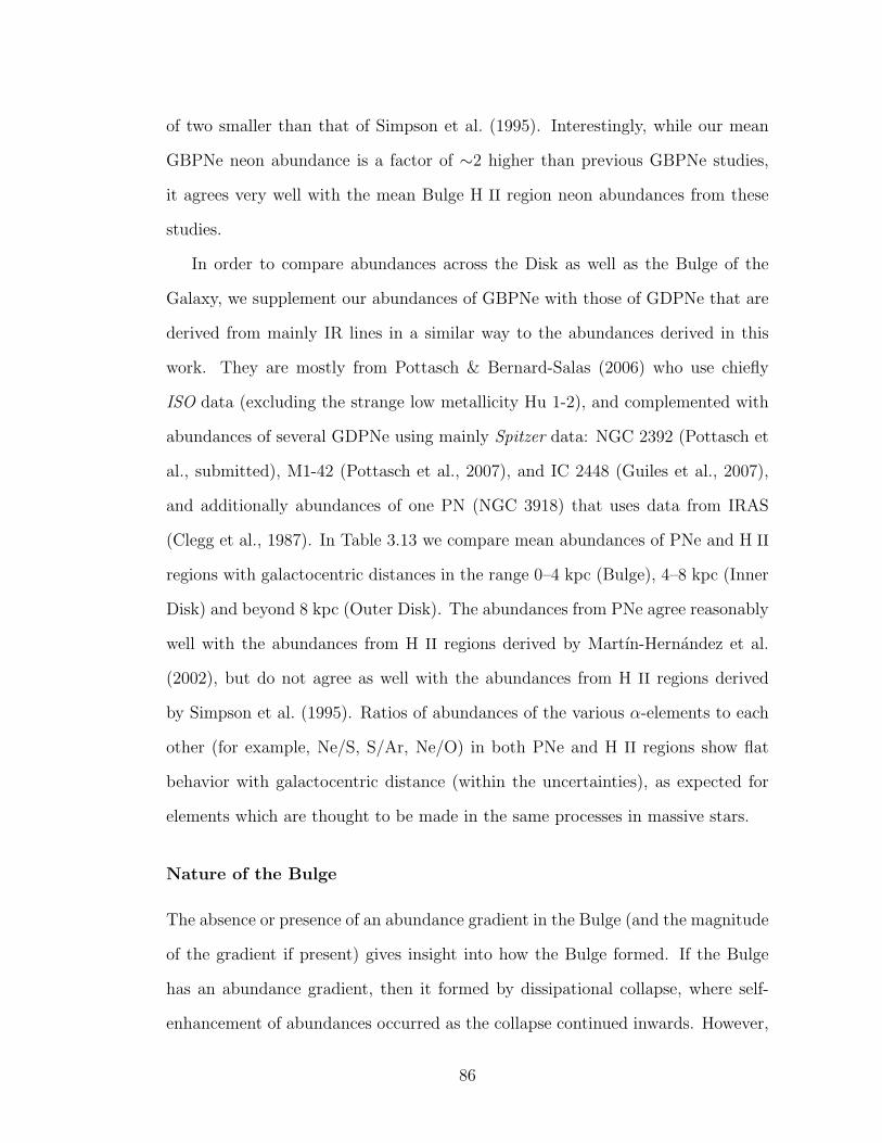
of two smaller than that of Simpson et al. (1995). Interestingly, while our mean

GBPNe neon abundance is a factor of ∼2 higher than previous GBPNe studies,

it agrees very well with the mean Bulge H II region neon abundances from these

studies.

In order to compare abundances across the Disk as well as the Bulge of the

Galaxy, we supplement our abundances of GBPNe with those of GDPNe that are

derived from mainly IR lines in a similar way to the abundances derived in this

work. They are mostly from Pottasch & Bernard-Salas (2006) who use chiefly

ISO data (excluding the strange low metallicity Hu 1-2), and complemented with

abundances of several GDPNe using mainly Spitzer data: NGC 2392 (Pottasch et

al., submitted), M1-42 (Pottasch et al., 2007), and IC 2448 (Guiles et al., 2007),

and additionally abundances of one PN (NGC 3918) that uses data from IRAS

(Clegg et al., 1987). In Table 3.13 we compare mean abundances of PNe and H II

regions with galactocentric distances in the range 0–4 kpc (Bulge), 4–8 kpc (Inner

Disk) and beyond 8 kpc (Outer Disk). The abundances from PNe agree reasonably

well with the abundances from H II regions derived by Martın-Hernandez et al.

(2002), but do not agree as well with the abundances from H II regions derived

by Simpson et al. (1995). Ratios of abundances of the various α-elements to each

other (for example, Ne/S, S/Ar, Ne/O) in both PNe and H II regions show flat

behavior with galactocentric distance (within the uncertainties), as expected for

elements which are thought to be made in the same processes in massive stars.

Nature of the Bulge

The absence or presence of an abundance gradient in the Bulge (and the magnitude

of the gradient if present) gives insight into how the Bulge formed. If the Bulge

has an abundance gradient, then it formed by dissipational collapse, where self-

enhancement of abundances occurred as the collapse continued inwards. However,

86

Table 3.13 Abundances of PNe and H II regions across the Galaxy. Obtain abun-dances relative to hydrogen by multiplying the numbers in the Table by 10x wherex is -6 for argon, -4 for neon, -5 for sulfur, and -4 for oxygen.

Distance range Ar/H Ne/H S/H O/H(kpc)

PNe: This work + others (see §3.6.1)0–4 4.6 2.7 1.2 4.54–8 4.3 1.9 1.2 5.08–... 2.7 1.1 0.63 4.2

H II Regions: Simpson et al. (1995)0–4 ... 2.5 2.7 124–8 ... 1.5 1.2 5.68–... ... 0.68 0.76 3.6

H II Regions: Martın-Hernandez et al. (2002)0–4 7.9 2.4 1.1 ...4–8 4.7 2.2 0.89 ...8–... 2.6 1.2 0.65 ...

if the Bulge does not have an abundance gradient, then it formed by dissipationless

collapse, where mergers of small protogalactic pieces caused an inhomogeneous

collapse over a long period of time and the mergers mixed stars of different ages

and metallicities. If the Bulge has only a shallow abundance gradient, then the

gravitational potential of the bar in our Galaxy caused concentrated star formation

at its center and the stars eventually left the Disk to become (part of) the Bulge

(Minniti et al., 1995).

Several (mainly optical) studies of GBPNe point toward a slightly more metal-

rich Bulge than Disk (Ratag et al., 1992; Cuisinier et al., 2000; Gorny et al., 2004;

Wang & Liu, 2007). However, Ratag et al. (1992) find that the average abundances

of GBPNe cannot be predicted by the abundance gradient observed for GDPNe,

hinting that stars in the Bulge are a distinct population from the Disk. Addition-

ally, Gorny et al. (2004) find that the O/H gradient becomes shallower and may

even decrease in the most inner parts of the Disk based on their sample of GDPNe

87

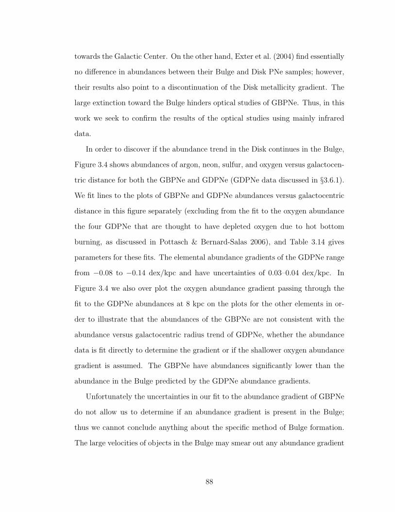
towards the Galactic Center. On the other hand, Exter et al. (2004) find essentially

no difference in abundances between their Bulge and Disk PNe samples; however,

their results also point to a discontinuation of the Disk metallicity gradient. The

large extinction toward the Bulge hinders optical studies of GBPNe. Thus, in this

work we seek to confirm the results of the optical studies using mainly infrared

data.

In order to discover if the abundance trend in the Disk continues in the Bulge,

Figure 3.4 shows abundances of argon, neon, sulfur, and oxygen versus galactocen-

tric distance for both the GBPNe and GDPNe (GDPNe data discussed in §3.6.1).

We fit lines to the plots of GBPNe and GDPNe abundances versus galactocentric

distance in this figure separately (excluding from the fit to the oxygen abundance

the four GDPNe that are thought to have depleted oxygen due to hot bottom

burning, as discussed in Pottasch & Bernard-Salas 2006), and Table 3.14 gives

parameters for these fits. The elemental abundance gradients of the GDPNe range

from −0.08 to −0.14 dex/kpc and have uncertainties of 0.03–0.04 dex/kpc. In

Figure 3.4 we also over plot the oxygen abundance gradient passing through the

fit to the GDPNe abundances at 8 kpc on the plots for the other elements in or-

der to illustrate that the abundances of the GBPNe are not consistent with the

abundance versus galactocentric radius trend of GDPNe, whether the abundance

data is fit directly to determine the gradient or if the shallower oxygen abundance

gradient is assumed. The GBPNe have abundances significantly lower than the

abundance in the Bulge predicted by the GDPNe abundance gradients.

Unfortunately the uncertainties in our fit to the abundance gradient of GBPNe

do not allow us to determine if an abundance gradient is present in the Bulge;

thus we cannot conclude anything about the specific method of Bulge formation.

The large velocities of objects in the Bulge may smear out any abundance gradient

88

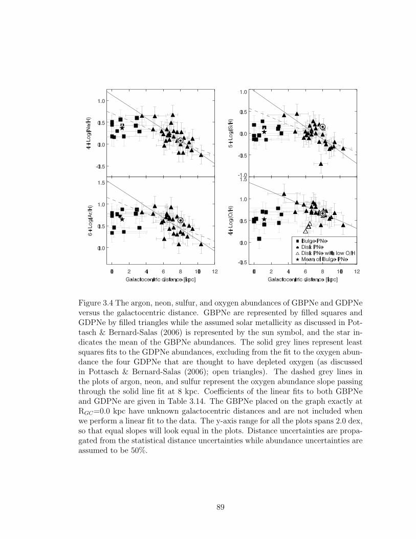
Figure 3.4 The argon, neon, sulfur, and oxygen abundances of GBPNe and GDPNeversus the galactocentric distance. GBPNe are represented by filled squares andGDPNe by filled triangles while the assumed solar metallicity as discussed in Pot-tasch & Bernard-Salas (2006) is represented by the sun symbol, and the star in-dicates the mean of the GBPNe abundances. The solid grey lines represent leastsquares fits to the GDPNe abundances, excluding from the fit to the oxygen abun-dance the four GDPNe that are thought to have depleted oxygen (as discussedin Pottasch & Bernard-Salas (2006); open triangles). The dashed grey lines inthe plots of argon, neon, and sulfur represent the oxygen abundance slope passingthrough the solid line fit at 8 kpc. Coefficients of the linear fits to both GBPNeand GDPNe are given in Table 3.14. The GBPNe placed on the graph exactly atRGC=0.0 kpc have unknown galactocentric distances and are not included whenwe perform a linear fit to the data. The y-axis range for all the plots spans 2.0 dex,so that equal slopes will look equal in the plots. Distance uncertainties are propa-gated from the statistical distance uncertainties while abundance uncertainties areassumed to be 50%.

89

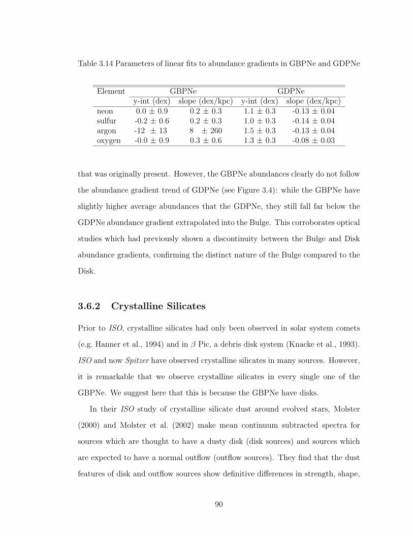
Table 3.14 Parameters of linear fits to abundance gradients in GBPNe and GDPNe

Element GBPNe GDPNey-int (dex) slope (dex/kpc) y-int (dex) slope (dex/kpc)

neon 0.0 ± 0.9 0.2 ± 0.3 1.1 ± 0.3 -0.13 ± 0.04sulfur -0.2 ± 0.6 0.2 ± 0.3 1.0 ± 0.3 -0.14 ± 0.04argon -12 ± 13 8 ± 260 1.5 ± 0.3 -0.13 ± 0.04oxygen -0.0 ± 0.9 0.3 ± 0.6 1.3 ± 0.3 -0.08 ± 0.03

that was originally present. However, the GBPNe abundances clearly do not follow

the abundance gradient trend of GDPNe (see Figure 3.4): while the GBPNe have

slightly higher average abundances that the GDPNe, they still fall far below the

GDPNe abundance gradient extrapolated into the Bulge. This corroborates optical

studies which had previously shown a discontinuity between the Bulge and Disk

abundance gradients, confirming the distinct nature of the Bulge compared to the

Disk.

3.6.2 Crystalline Silicates

Prior to ISO, crystalline silicates had only been observed in solar system comets

(e.g. Hanner et al., 1994) and in β Pic, a debris disk system (Knacke et al., 1993).

ISO and now Spitzer have observed crystalline silicates in many sources. However,

it is remarkable that we observe crystalline silicates in every single one of the

GBPNe. We suggest here that this is because the GBPNe have disks.

In their ISO study of crystalline silicate dust around evolved stars, Molster

(2000) and Molster et al. (2002) make mean continuum subtracted spectra for

sources which are thought to have a dusty disk (disk sources) and sources which

are expected to have a normal outflow (outflow sources). They find that the dust

features of disk and outflow sources show definitive differences in strength, shape,

90

Figure 3.5 Normalized and shifted mean 28 and 33 µm spectra of our GBPNecompared to the mean disk and outflow sources from Molster et al. (2002).

and position of their dust features. In Figure 3.5 we plot normalized mean spectra

of our GBPNe for the 28 and 33 µm features and compare them to the normalized

mean disk and outflow spectra from Molster et al. (2002). Both the 28 and 33

µm complexes in our GBPNe look similar to the mean disk sources in Molster

et al. (2002), but Molster et al. (2002) have several cautions about their mean

spectra (for example, the ISO SWS band 3E, which covers the ∼27.5–29.2 µm, is

known to have less reliable calibration). However, the similarity of the crystalline

silicate dust features in our GBPNe to those of Molster’s disk sources gives indirect

evidence that the silicates in our GBPNe are in disks.

If the crystalline silicates in these GBPNe are in fact in disks, then they point

toward binary evolution of the progenitor stars. Edgar et al. (2007) ran numerical

91

models that show how a binary companion can shape the AGB wind to form

a crystalline dust torus. In their models, the shock temperatures reached when

the wind blows past the companion anneal the dust and make it crystalline. They

conclude that “Crystalline dust torii provide strong evidence for binary interactions

in AGB winds.” As we discuss later in §3.6.4, over half of the GBPNe in this study

show dual chemistry, which also implies binary evolution.

In our GBPNe sample, all of the nebulae show crystalline silicates, indicative

of oxygen-rich material. Previous studies have found a low C/O ratio in GBPNe

compared to GDPNe (e.g. Walton et al., 1993a; Wang & Liu, 2007; Casassus et al.,

2001). The higher fraction of O-rich PNe in the Bulge compared to the Disk implies

that the Bulge should have a larger injection of silicate grains into its interstellar

medium (ISM) than the Disk (Casassus et al., 2001).

3.6.3 PAHs

PAHs can be separated into different classes based on the position of their 6.2 µm

and 7.7 µm peaks. Class A PAHs peak at shorter wavelengths than class B, which

peak at shorter wavelengths than class C (Peeters et al., 2002). Figure 3.3 shows

the peak positions for the different classes of PAHs along with the GBPNe PAH

features. The GBPNe in this study have class A, AB, and B PAHs, and thus have

PAH profiles similar to GDPNe. The lack of type C PAHs in the PNe indicates

that their PAHs are all processed, i.e. the aliphatic component is negligible (Sloan

et al., 2007).

The PAH flux ratios F7.7µm/F11.2µm and F6.2µm/F11.2µm both trace the ioniza-

tion fraction of the PAHs, and are often plotted against each other in a figure. The

GBPNe studied here have F7.7µm/F11.2µm between 1 and 3, and F6.2µm/F11.2µm

between 0.5 and 1.4, and follow the same trend as Galactic Disk and Magellanic

92

Cloud PNe (Bernard-Salas et al., in preparation).

3.6.4 Dual Chemistry Nebulae

ISO detected crystalline silicates and PAHs simultaneously in [WR] PNe — those

PNe with H-poor and C-rich WR-type central stars (Waters et al., 1998). This

dual chemistry is unusual in GDPNe (Bernard-Salas & Tielens, 2005). However,

in our sample of GBPNe, six of the eleven nebulae have dual chemistry, showing

both crystalline silicates and PAHs in their spectra. The fraction of [WR] PNe is

significantly larger in the Bulge than the Disk (Gorny et al., 2004), and thus the

large fraction of PNe in the Bulge exhibiting dual chemistry makes sense. Possible

explanations for this dual chemistry include (Little-Marenin, 1986; Willems & de

Jong, 1986; Waters et al., 1998; Cohen et al., 1999): (1) a thermal pulse recently

(. 1000 years ago) turned an O-rich outflow into a C-rich one, and (2) the central

star of the PN is in a binary system and the silicate grains orbit the system in a

disk that existed long before the PN.

What explains how the majority of our GBPNe show dual chemistry? The

explanation of a thermal pulse at the end of the AGB having suddenly changed

the chemical composition of the central star from O-rich to C-rich within the last

thousand years seems implausible because it is unlikely that we would catch so

many GBPNe in this short stage (e.g. Lloyd Evans, 1991). A growing body of

evidence supports the binary system with an old silicate disk explanation of dual

chemistry in PNe and late-type stars (Waters et al., 1998; Molster et al., 2001;

Matsuura et al., 2004). Taking one of these studies as an example, Matsuura et al.

(2004) present mid-IR images of the post-AGB star IRAS 16279-4757 which shows

both PAHs and crystalline silicates. Their images and model of this star imply that

it has a C-rich bipolar outflow with an inner low-density C-rich region surrounded

93

by an outer dense O-rich torus, indicating that mixed chemistry and morphology

are related; mixed chemistry may point to binary evolution.

Other evidence also suggests that many of our GBPNe probably have binaries

with silicate disks: (1) ∼40% of compact PNe in the Bulge have binary-induced

morphologies (Zijlstra, 2007); (2) binary-induced novae are observed to be concen-

trated in the bulge of the galaxy M31 (e.g. Shafter & Irby, 2001; Rosino, 1973),

and thus perhaps in the Bulge of our galaxy as well; (3) asymmetric (e.g. bipolar,

quadrupolar) morphology is more common in PNe in high metallicity environ-

ments than in low metallicity ones (Stanghellini et al., 2003); (4) the current study

showing the similarity of the mean GBPNe spectra to the mean disk spectra of

Molster et al. 2002 (§3.6.2); and (5) the silicates are crystalline and not amor-

phous, indicating that they have been blasted over time and are likely stored in

a disk (Molster et al., 1999). Thus it seems likely that the GBPNe in our sample

with dual chemistry have a binary at their center with a silicate disk that formed

long before the PN stage, while the PAHs reside in the PN outflow itself, possibly

shooting out along the poles.

3.7 Conclusions

We extract the Spitzer IRS spectra of eleven PNe in the Bulge to study their

abundances and dust properties. We conclude that:

(1) The abundances of argon, neon, sulfur, and oxygen are significantly lower

in the PNe in the Bulge than the abundances for the Bulge predicted by the

abundance gradient in the Disk, consistent with the idea that the Bulge and Disk

evolved separately.

(2) All of the spectra in our sample of PNe in the Bulge show crystalline sil-

icates, indicating that these crystalline silicates are likely stored in disks, which

94

would further imply that the progenitor stars of these PNe evolved in binary sys-

tems.

(3) Six of the eleven spectra of PNe in the Bulge in our sample show PAHs in

addition to the crystalline silicates. This dual chemistry also points toward binary

evolution: the PAHs are in the current PN outflow and the crystalline silicates

reside in a old disk created by binary interaction.

This work is based in part on observations made with the Spitzer Space Tele-

scope, which is operated by the Jet Propulsion Laboratory, California Institute of

Technology under NASA contract 1407. Support for this work was provided by

NASA through Contract Number 1257184 issued by JPL/Caltec. This research

made use of the SIMBAD database, operated at CDS, Strasbourg, France.

95

CHAPTER 4

ABUNDANCES IN H II REGIONS ACROSS M51 FROM SPITZER

SPECTRA

4.1 Introduction

Determining the elemental abundances of H II regions across disks of spiral galaxies

gives important information about how they formed and evolved (see Chapter 1).

However, only a small number of galaxies have direct measurements of abundances

in H II regions across their entire disks, including the metal-rich nuclear regions,

because it is difficult to detect the faint optical lines necessary for determining

the electron temperature in these metal-rich regions. Thus astronomers employ

indirect methods for determining abundances across external galaxies, such as the

R23 method (Pagel et al., 1979) which relies on an empirical relation between strong

line fluxes and abundances. These indirect methods imply abundances significantly

above solar at the centers of many nearby spiral galaxies.

In this chapter we seek to employ data from the Spitzer Space Telescope (Werner

et al., 2004) Infrared Spectrograph (IRS; Houck et al., 2004) in order to de-

rive abundances from twelve H II regions across the galaxy M51, which has been

thought to have a high central abundance since the early 1990’s. For example,

Vila-Costas & Edmunds (1992) inferred abundances of 15 H II regions across M51

from the empirical strong-line R23 method, finding an abundance gradient of -0.06

dex/kpc and a predicted oxygen abundance at the center of 12 + log(O/H) = 9.54

dex (7.5 × O/H¯, adopting (O/H)¯ = 4.6 × 10−4 from Asplund et al. (2005)).

They also found abundances greater than solar in all of the observed H II re-

gions. Additionally, Diaz et al. (1991) employed spectrophotometric observations

and theoretical photoionization models to indirectly determine abundances for six

96

giant H II regions across M51, and found abundances for these regions from 2.8 to

5.5 × (O/H)¯.

Recently however, Bresolin et al. (2004) took deep optical spectra of several

metal-rich H II regions within M51. They detected the faint lines necessary for

determining the electron temperature, and thus were able to directly determine

abundances. Their abundances for H II regions in M51 are the most accurate to

date because they do not rely on indirect methods. Such direct determinations of

the abundances give important information relevant to understanding how galaxies

form and evolve as well as providing a check on indirect calculations of abundances.

Strikingly, Bresolin et al. (2004) find that the oxygen abundances of the central

metal-rich H II regions in M51 are a factor of several lower than found by the above

studies (Diaz et al., 1991; Vila-Costas & Edmunds, 1992) which employ indirect

methods. This finding suggests a flatter abundance gradient across M51 and im-

plies that the empirical determination of abundances from strong lines may be in

error, perhaps due to problems in the theoretical models employed in calibrating

the indirect methods. In the ideal case we could directly determine abundances

from lines in Spitzer infrared spectra of H II regions across M51 and test the results

of Bresolin et al. (2004).

M51 (a.k.a. NGC 5194 and the Whirlpool) is a famous nearly face-on (incli-

nation = 20, Tully, 1974) grand-design spiral galaxy at a distance of 8.4 Mpc

(Feldmeier et al., 1997). It was the first galaxy where the spiral structure was

noticed (by Lord Rosse in 1845; Bailey et al., 2005), and the pronounced spiral

structure is probably due to the tidal interaction with its companion galaxy, NGC

5195 (Salo & Laurikainen, 2001). Additionally, M51 harbors a supermassive black

hole in its nucleus (Crane & van der Hulst, 1992).

Neon and sulfur are made in the α-process in massive stars, and thus we would

97

expect their abundance ratio to remain constant across a galaxy. IRS spectra of

H II regions may show lines from ions of Ne+, Ne++, S++, and S3+. These are the

dominant ions which contribute to the neon and sulfur abundances in most H II

regions, and thus we can estimate the total neon to sulfur ratio from these lines to

see if it remains constant or varies across the galaxy. Rubin et al. (2007) made a

similar study employing IRS data on H II regions across the galaxy M83.

In the following section (§4.2) we describe the observations and data reduction

of both the Spitzer IRS maps and the Hα map. We derive abundances in §4.3.

§4.4 gives our results about the hardness of the radiation field and the neon to

sulfur abundance ratio across M51, and we summarize what we learned in §4.5.

4.2 Observations and Data Reduction

4.2.1 Spitzer Data

For the present study we analyze the spectral maps of H II regions across M51

taken with Spitzer IRS by the Spitzer Infrared Nearby Galaxies Survey (SINGS)

team (Kennicutt et al., 2003)1. Specifically, we employ their Short-High module

maps which cover the wavelength range from 10 to 19 µm at a resolution of R ∼600. This wavelength range includes lines from Ne II, Ne III, Ne V, S III, and S IV.

The data were taken in ‘mapping mode’ with an integration time of 30 seconds ×2 cycles. The map was made by stepping the slit across each H II region in half-slit

sized steps for redundancy in order to reduce the affects of under-sampling and

issues with diffraction2. Figure 4.1 shows IRS slit overlays on the SINGS Hα map

of M51. Table 4.1 lists the central positions of each H II region mapped, indexed

by the letter (A–L) which labels each mapped H II region in Figure 4.1.

1SINGS team website: http://sings.stsci.edu/2For details see: http://ssc.spitzer.caltech.edu/irs/documents/specmap bop/

98

Figure 4.1 SINGS Hα continuum subtracted image of M51 with overlays of the SHIRS maps. The region mapped by the IRS at the top of the image is NGC5195,the companion galaxy to M51.

99

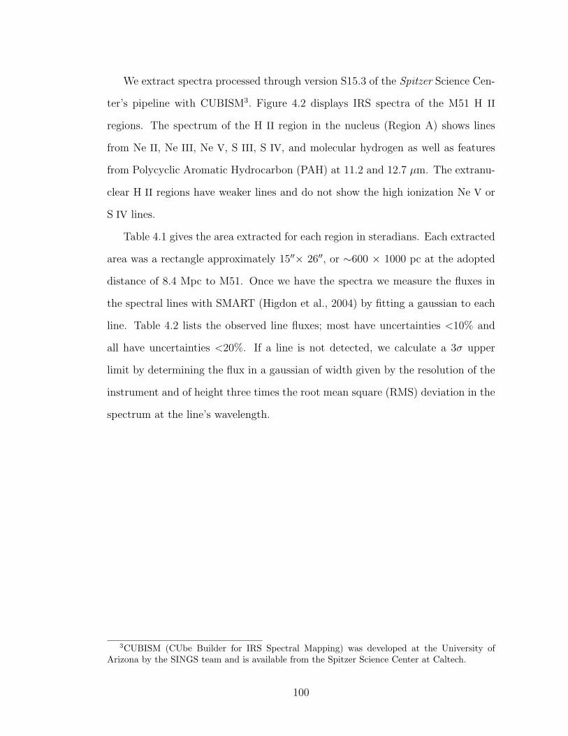
We extract spectra processed through version S15.3 of the Spitzer Science Cen-

ter’s pipeline with CUBISM3. Figure 4.2 displays IRS spectra of the M51 H II

regions. The spectrum of the H II region in the nucleus (Region A) shows lines

from Ne II, Ne III, Ne V, S III, S IV, and molecular hydrogen as well as features

from Polycyclic Aromatic Hydrocarbon (PAH) at 11.2 and 12.7 µm. The extranu-

clear H II regions have weaker lines and do not show the high ionization Ne V or

S IV lines.

Table 4.1 gives the area extracted for each region in steradians. Each extracted

area was a rectangle approximately 15′′× 26′′, or ∼600 × 1000 pc at the adopted

distance of 8.4 Mpc to M51. Once we have the spectra we measure the fluxes in

the spectral lines with SMART (Higdon et al., 2004) by fitting a gaussian to each

line. Table 4.2 lists the observed line fluxes; most have uncertainties <10% and

all have uncertainties <20%. If a line is not detected, we calculate a 3σ upper

limit by determining the flux in a gaussian of width given by the resolution of the

instrument and of height three times the root mean square (RMS) deviation in the

spectrum at the line’s wavelength.

3CUBISM (CUbe Builder for IRS Spectral Mapping) was developed at the University ofArizona by the SINGS team and is available from the Spitzer Science Center at Caltech.

100

Tab

le4.

1M

51H

IIre

gion

dat

a

Reg

ion

Coor

din

ates

(J20

00)

Obse

rved

Hα

flux

aE

xtr

acte

dA

reab

Avc

Te(K

)d

RA

DE

C(×

10−1

3)

erg

cm−2

s−1

sr−1

(×10−8

)sr

Te(N

eII

,S

III)

Te(N

eII

I,S

IV)

A13

2952

.747

1143

21.0

1.17

4.00

6600

e58

00e

B13

2949

.747

1329

0.56

1.17

...

6600

e58

00e

C13

2956

.747

1046

2.32

1.17

2.17

6600

e58

00e

D13

2956

.247

1407

2.20

1.17

2.61

6400

f56

00f

E13

2959

.647

1402

5.68

1.27

1.01

6400

5600

F13

2939

.547

0836

3.46

1.16

2.24

7300

6800

G13

3002

.547

0952

6.78

1.36

0.91

6200

g54

00g

H13

2959

.847

1113

2.50

1.36

3.11

6600

e58

00e

I13

3001

.647

1252

3.60

1.17

3.57

6600

e58

00e

J13

2953

.147

1240

2.49

1.17

1.78

4800

3700

K13

2944

.247

1022

7.69

1.27

1.93

5700

4600

L13

2944

.647

0955

7.93

1.36

1.64

5700

f46

00f

aO

bser

ved

Hα

flux

from

the

regi

onex

trac

ted

byC

UB

ISM

for

each

HII

regi

onas

disc

usse

din§4

.2.2

.bR

ecta

ngul

arar

eace

nter

edon

each

HII

regi

onan

dex

trac

ted

wit

hC

UB

ISM

;al

lar

eas∼1

5×

26′′

or∼6

00×

1000

pc.

cE

xtin

ctio

nsfr

omva

nde

rH

ulst

etal

.(19

88)

from

Hα/r

adio

.Fo

rtw

ore

gion

s(E

and

J)th

eIR

Sm

apco

vere

dse

vera

lHII

regi

ons

ofva

nde

rH

ulst

etal

.(1

988)

and

inth

ese

case

sth

eA

vis

the

aver

age

ofth

eex

tinc

tion

sfr

omth

eco

vere

dre

gion

s.dTem

pera

ture

sfr

omB

reso

linet

al.(2

004)

.eT

eis

the

aver

age

from

the

sam

ple

ofB

reso

linet

al.(2

004)

.fT

eis

from

ane

arby

HII

regi

on.

Te

for

regi

onD

isfr

omre

gion

E;T

efo

rre

gion

Lis

from

regi

onK

.gR

egio

nG

cove

rsth

ere

gion

s53

and

55in

Bre

solin

etal

.(2

004)

and

thus

we

aver

age

thos

ete

mpe

ratu

res.

101

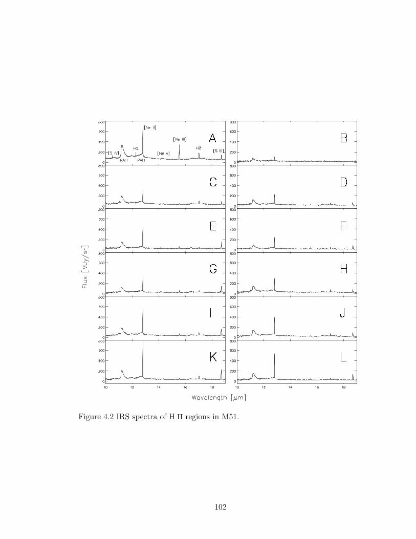
Figure 4.2 IRS spectra of H II regions in M51.

102

Table 4.2 M51 H II region line fluxes. Uncertainties are less than 10% unlessotherwise noted. A less-than sign indicates a 3σ upper limit as discussed in §4.2.1.

Region Observed line fluxes (10−6 erg cm−2 s−1 sr−1 )S IV Ne II Ne V Ne III S III

10.51 µm 12.81 µm 14.32 µm 15.55 µm 18.71 µmA 23 278 8.9a 106 28B <42 34 <21 <25 <25C <33 111 <21 7.7a 16a

D <27 68 <16 7.9a 16E <36 150 <20 15 38F <30 89 <15 15a 23G <33 134 <19 15 34H <38 110 <20 6.7a 20I <34 189 <19 11a 41J <40 128 <16 6.2b 22K <43 276 <20 9.3 58L <41 186 <17 15 34

aUncertainty between 10 and 15%.bUncertainty between 15 and 20%.

4.2.2 Hα Map

This project originated out of a pilot effort to assess the feasibility of determining

the abundances of H II regions across several galaxies from Spitzer IRS maps of

these galaxies made by the IRS team here at Cornell and the SINGS team. Unfor-

tunately, none of these IRS maps were deep enough for the hydrogen recombination

lines to be observed in the spectra (the strongest H I line with a wavelength in the

range of the SH module of the IRS being the H I(7-6) line at 12.36 µm). Thus we

made observations of these galaxies with the Wide-field InfraRed Camera (WIRC)

on the Palomar 200” Hale Telescope in the Br-γ and Pa-β H I lines in order to

determine the amount of hydrogen as well as the extinction in the IRS slits. Un-

fortunately we were unable to accurately determine the amount of hydrogen in the

103

IRS slits from these WIRC observations due to a combination of cloudy weather

and the difficulty of obtaining a sufficiently high signal-to-noise ratio in the H I

lines for the fainter H II regions.

As an alternate approach, we looked through the subset of galaxies mapped by

the IRS that had an optical H I map and extinctions to the individual H II regions

given in the literature. However, this approach has the problem that we must

rely on optical measurements which are more affected by extinction and also on

extinction values computed from different apertures than the area of the extracted

IRS maps. We chose the galaxy M51 for this study because it had an Hα map

made by the SINGS team (see Figure 4.1) and extinctions given in the literature

to all but one of the H II regions mapped with the IRS.

We tried two methods for determining the background in the SINGS Hα map:

(1) adopting a sky annulus chosen so that it does not fall on nearby H II regions,

and (2) adopting a constant background determined from the average of the four

corners of the array (where there is less contamination from H II regions in the

galaxy). The two different types of background subtraction gave Hα fluxes that

agreed within 50%. We tested the sky subtraction methods by using them both to

determine the Hα fluxes in circular apertures of 6.5′′ radius. We then compared

these Hα flux values with those for the same apertures published by the SINGS

team (Calzetti et al., 2005) who adopted a background subtraction method which

involved fitting a local background in each of twelve areas across the map and

would be difficult to duplicate. The sky annulus did the best job of reproducing

the Calzetti et al. (2005) results, with our Hα flux values often within 20% of theirs

(and almost all within a factor of 2), thus we adopt this sky subtraction method.

Due to the uncertainty in determining the amount of hydrogen in the extracted

area of the IRS maps from the Hα map and also the uncertainty in determining

104

the extinctions, unfortunately we are unable to determine accurate abundances

with respect to hydrogen, although we describe the process below. However, we

can determine more accurate abundance ratios because in such ratios the amount

of hydrogen cancels out.

4.3 Data Analysis

4.3.1 Extinction Correction

We adopt extinctions for M51 H II regions from van der Hulst et al. (1988). They

used 6 cm and 20 cm observations to determine the thermal radio emission and

then determined the extinction from the Hα to radio ratio. Depending on the size

of the H II region, they used apertures from 12′′ to 21′′ in diameter. Additionally,

they did 9′′-aperture optical spectrophotometry on several H II regions and thus

also determined Balmer-decrement extinctions for a subset of H II regions with

Hα/radio extinctions. Table 4.1 lists the Av values we adopt for determining

abundances.

4.3.2 Electron Temperature and Density

Table 4.1 also lists the temperatures for each region adopted for determining abun-

dances. They are from Bresolin et al. (2004). The Te(Ne II, S III) is the tempera-

ture we adopt for determining abundances from Ne II and S III line fluxes; similarly,

the Te(Ne III, S IV) is the temperature we adopt for determining abundances from

Ne III and S IV line fluxes. The Te(Ne II, S III) we adopt is equal to Te(S+2, Ar+2)

from Bresolin et al. (2004) because the ionization potential of Ne II (21.56eV) is

close to that of S III (23.34eV) and Ar III (27.63eV). Similarly, the Te(Ne III,

105

S IV) we employ is equal to Te(O+2, Ne+2) of Bresolin et al. (2004) because the

ionization potential of S IV (34.79eV) is close to that of O III (35.12eV) and Ne III

(40.96eV). When Bresolin et al. (2004) do not give Te for a given H II region,

we adopt the average temperature from their sample. However, if an H II region

without a Te given by Bresolin et al. (2004) resides nearby another H II region

with Te given, then we adopt the Te of the nearby region. Abundances derived

from infrared lines depend only weakly on Te, and thus choosing an average Te or

one from a nearby H II region will have little affect on the abundances.

For the electron density we assume Ne = 100 cm−3 for all H II regions in M51.

Bresolin et al. (2004) determined that Ne < 150 cm−3 for the H II regions in M51,

and the adopted electron density does not have a large affect on the abundances.

4.3.3 Abundances

We assume the above Hα flux, extinction, electron temperatures and density in

order to derive the abundances for each ion, following the procedure outlined in

§1.3.3. Our procedure employs the Hβ flux, so here we predict the observed Hβ

flux from the Hα flux by using the theoretical ratio of (Hα flux)/(Hβ flux) = 3.0

for case B recombination for a gas at Te=5000 K and Ne= 100 cm−3 from Hummer

& Storey (1987) and the extinction given in Table 4.1. Table 4.3 lists the ionic

abundances (and upper limits for unobserved ions) for three ions of neon and two

ions of sulfur. These abundances with respect to hydrogen should be viewed with

caution because the Hα flux has a large uncertainty; however, ratios of abundances

will not be affected.

106

Tab

le4.

3A

bundan

ces

inM

51H

IIre

gion

s.

Reg

ion

Ne+

Ne+

+N

e+4

S+

+S

+3

Ne+

+N

e++

S+

++

S+

3

12.8

1µm

15.5

5µm

14.3

2µm

18.7

1µm

10.5

1µm

(×10−3

)(×

10−5

)(×

10−6

)(×

10−5

)(×

10−6

)(×

10−3

)(×

10−5

)A

0.29

5.25

0.43

0.29

0.42

0.34

0.33

C1.

023.

36<

8.93

1.51

<5.

051.

051.

51D

0.67

3.70

<7.

311.

56<

4.56

0.71

1.56

E1.

235.

96<

7.60

3.13

<4.

751.

293.

13F

1.03

8.24

<8.

752.

55<

5.56

1.11

2.55

G1.

306.

75<

8.26

3.31

<5.

081.

373.

31H

1.11

3.23

<9.

362.

01<

6.51

1.14

2.01

I1.

143.

21<

5.42

2.45

<3.

591.

172.

45J

1.24

2.86

<6.

352.

22<

6.55

1.27

2.22

K1.

482.

38<

4.80

3.19

<3.

761.

503.

19L

0.61

2.41

<2.

401.

12<

2.24

0.63

1.12

107

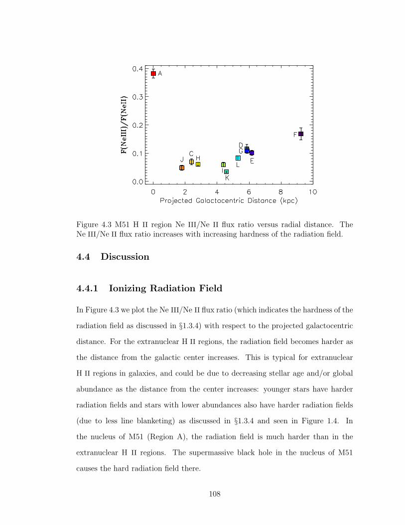
Figure 4.3 M51 H II region Ne III/Ne II flux ratio versus radial distance. TheNe III/Ne II flux ratio increases with increasing hardness of the radiation field.

4.4 Discussion

4.4.1 Ionizing Radiation Field

In Figure 4.3 we plot the Ne III/Ne II flux ratio (which indicates the hardness of the

radiation field as discussed in §1.3.4) with respect to the projected galactocentric

distance. For the extranuclear H II regions, the radiation field becomes harder as

the distance from the galactic center increases. This is typical for extranuclear

H II regions in galaxies, and could be due to decreasing stellar age and/or global

abundance as the distance from the center increases: younger stars have harder

radiation fields and stars with lower abundances also have harder radiation fields

(due to less line blanketing) as discussed in §1.3.4 and seen in Figure 1.4. In

the nucleus of M51 (Region A), the radiation field is much harder than in the

extranuclear H II regions. The supermassive black hole in the nucleus of M51

causes the hard radiation field there.

108

Figure 4.4 M51 (Ne++Ne++)/(S+++S3+) abundance ratio versus radial distance.

4.4.2 Neon to Sulfur Abundance Ratio

We do not plot the neon and sulfur abundances versus radial distance because

the uncertainties (mainly due to calculating the amount of H+ in the same re-

gion mapped with the IRS) on them are so large that they yield a scatter plot.

(Comparing neon and sulfur abundances for regions in common with Bresolin

et al. (2004) we are off by factors of a few.) Fortunately, the uncertainty on their

abundance ratio is much smaller. Because we observe the dominant ionization

states of neon and sulfur in these H II regions, we may approximate Ne/S by

(Ne++Ne++)/(S+++S3+). We only observe the high ionization stage Ne+4 in the

central H II region, and even there the abundance of Ne+4 is negligible compared

to the abundances of Ne+ and Ne++, and we think that the sum of Ne++Ne++

should reliably trace the total neon abundance. However, none of the extranuclear

regions have S3+ observed, and thus they are all relatively low excitation and S+

may contribute significantly to their total sulfur abundance.

109

Figure 4.4 shows a plot of the (Ne++Ne++)/(S+++S3+) abundance ratio versus

projected galactocentric distance. We assume that uncertainties in the line fluxes

dominate this abundance ratio and propagate the uncertainties accordingly. We

find that the Ne/S abundance ratio seems to decrease with increasing galactocen-

tric radius. One would expect the Ne/S abundance ratio to be constant because

both neon and sulfur are made in the same processes in massive stars. However, S+

is not included in our trace of the Ne/S ratio, and S+ probably contributes more

to the total sulfur abundance in the inner H II regions that have softer radiation

fields (see Figure 4.3); in addition, the inner metal-rich H II regions probably have

a higher amount of dust (Sandford et al., 1995), which could lower the measured

total sulfur abundance there because sulfur may be depleted onto the dust (while

neon would not be depleted because it is chemically inert). Given these considera-

tions, (Ne++Ne++)/(S+++S3+) probably gives an upper limit to the total neon to

sulfur ratio. Rubin et al. (2007) also studied the neon to sulfur ratio as traced by

(Ne++Ne++)/(S+++S3+) for H II regions across the galaxy M83 and found similar

results, namely that Ne/S appeared to decrease with increasing radial distance.

4.5 Conclusions

We extracted Spitzer IRS spectra for twelve H II regions across the nearly face-

on spiral galaxy M51. We measured line fluxes or upper limits for the following

ions in each H II region: Ne+, Ne++, Ne+4, S++, and S+3; lines from the ions of

Ne+4 and S+3 were only observed in the nuclear H II region where a supermassive

black hole resides, causing a hard radiation field. Then we derived abundances (or

upper limits on the abundances) for these ions. However, we could not accomplish

the original goal of determining accurate elemental abundances with respect to

hydrogen across M51 because of the large uncertainty in the Hα flux within each

110

extracted area along with the added uncertainty from adopting an extinction from

a different sized aperture. We did find that in the extranuclear H II regions, the

hardness of the radiation field as traced by the Ne III/Ne II flux ratio increases as

the distance from the galactic center increases (attributed to decreasing abundance

and/or stellar age with increasing distance). Additionally, we found that the neon

to sulfur ratio as traced by (Ne++Ne++)/(S+++S3+) appears to decrease with

increasing distance from the nucleus, but this probably does not reflect a trend in

the true Ne/S ratio, but rather reflects the affect of not accounting for unobserved

S+ and/or depletion of sulfur onto dust.

In order to determine accurate Ne/H and S/H abundances from Spitzer IRS

spectra, it is necessary to measure the hydrogen within the IRS slit. The short

integration time of the SINGS maps (1 minute at each pointing with a maximum

integration time of 4 minutes at the center of the maps where the pointings overlap)

is not long enough to detect the H I(7-6) line in the SH module of the Spitzer

IRS. However, longer integration times of ∼15+ minutes do allow the detection

of this line in H II regions of external galaxies. For example, the program by

Robert Rubin (program ID 20057) makes small maps of H II regions in M33 with

a maximum integration time in the centers of the maps of 18 minutes, and they

detect the H I(7-6) line, usually above the 3σ limit (private communication). A

program by Fabio Bresolin (program ID 30205) does staring mode observations

of ten H II regions in nearby galaxies with a 26 minute integration time on each

region, and they should also detect the H I(7-6) line. Programs such as Rubin’s

and Bresolin’s with integration times long enough to detect the H I(7-6) line are

the way to determine accurate neon and sulfur abundances from infrared spectra

of H II regions across galaxies. Future investigators will be able to determine

abundances from infrared lines with the Mid-Infrared Instrument (MIRI) on the

111

James Webb Space Telescope (JWST); MIRI will provide high resolution (R ∼3000) spectroscopy from 5 to 28 µm and thus cover the H I(7-6) at 12.37 µm as

well as lines from important ionization stages of argon, neon, and sulfur.

112

BIBLIOGRAPHY

Acker, A., Marcout, J., Ochsenbein, F., Stenholm, B., & Tylenda, R. 1992, Stras-

bourg - ESO catalogue of galactic planetary nebulae. Part 1; Part 2 (Garching:

European Southern Observatory, 1992)

Acker, A., Raytchev, B., Koeppen, J., & Stenholm, B. 1991, A&AS, 89, 237

Allamandola, L. J., Tielens, G. G. M., & Barker, J. R. 1989, ApJS, 71, 733

Asplund, M., Grevesse, N., & Sauval, A. J. 2005, in ASP Conf. Ser. 336: Cosmic

Abundances as Records of Stellar Evolution and Nucleosynthesis, ed. T. G.

Barnes, III & F. N. Bash, 25–+

Bailey, M. E., Butler, C. J., & McFarland, J. 2005, Astronomy and Geophysics,

46, 26

Ballero, S. K., Matteucci, F., Origlia, L., & Rich, R. M. 2007, A&A, 467, 123

BBC. 2001

Beaulieu, S. F., Dopita, M. A., & Freeman, K. C. 1999, ApJ, 515, 610

Benjamin, R. A., Skillman, E. D., & Smits, D. P. 1999, ApJ, 514, 307

Bensby, T. & Lundstrom, I. 2001, A&A, 374, 599

Bernard-Salas, J. 2003, Physics and Chemistry of Gas in Planetary Nebulae (The-

sis, University of Groningen)

Bernard-Salas, J., Pottasch, S. R., Beintema, D. A., & Wesselius, P. R. 2001, A&A,

367, 949

Bernard-Salas, J., Pottasch, S. R., Gutenkunst, S., Morris, P. W., & Houck, J. R.

2008, ApJ, 672, 274

113

Bernard-Salas, J. & Tielens, A. G. G. M. 2005, A&A, 431, 523

Bernstein, R. A., Freedman, W. L., & Madore, B. F. 2002, ApJ, 571, 107

Berrington, K. A. 1985, Journal of Physics B: Atomic and Molecular Physics, 18,

L395

Berrington, K. A., Burke, P. G., Dufton, P. L., & Kingston, A. E. 1985, Atomic

Data and Nuclear Data Tables, 33, 195

Blum, R. D. & Pradhan, A. K. 1992, ApJS, 80, 425

Bresolin, F., Garnett, D. R., & Kennicutt, Jr., R. C. 2004, ApJ, 615, 228

Buonanno, R., Corsi, C. E., Pecci, F. F., Fahlman, G. G., & Richer, H. B. 1994,

ApJ, 430, L121+

Cahn, J. H., Kaler, J. B., & Stanghellini, L. 1992, A&AS, 94, 399

Calzetti, D., Kennicutt, Jr., R. C., Bianchi, L., Thilker, D. A., Dale, D. A., Engel-

bracht, C. W., Leitherer, C., Meyer, M. J., Sosey, M. L., Mutchler, M., Regan,

M. W., Thornley, M. D., Armus, L., Bendo, G. J., Boissier, S., Boselli, A.,

Draine, B. T., Gordon, K. D., Helou, G., Hollenbach, D. J., Kewley, L., Madore,

B. F., Martin, D. C., Murphy, E. J., Rieke, G. H., Rieke, M. J., Roussel, H.,

Sheth, K., Smith, J. D., Walter, F., White, B. A., Yi, S., Scoville, N. Z., Polletta,

M., & Lindler, D. 2005, ApJ, 633, 871

Carollo, D., Beers, T. C., Lee, Y. S., Chiba, M., Norris, J. E., Wilhelm, R., Sivarani,

T., Marsteller, B., Munn, J. A., Bailer-Jones, C. A. L., Fiorentin, P. R., & York,

D. G. 2007, Nature, 450, 1020

Carroll, B. W. & Ostlie, D. A. 1996, Institute for Mathematics and Its Applications

114

Casassus, S., Roche, P. F., Aitken, D. K., & Smith, C. H. 2001, MNRAS, 327, 744

Chiappini, C., Matteucci, F., & Gratton, R. 1997, ApJ, 477, 765

Chiappini, C., Romano, D., & Matteucci, F. 2003, MNRAS, 339, 63

Ciardullo, R., Bond, H. E., Sipior, M. S., Fullton, L. K., Zhang, C.-Y., & Schaefer,

K. G. 1999, AJ, 118, 488

Clegg, R. E. S., Harrington, J. P., Barlow, M. J., & Walsh, J. R. 1987, ApJ, 314,

551

Cohen, M., Barlow, M. J., Sylvester, R. J., Liu, X.-W., Cox, P., Lim, T., Schmitt,

B., & Speck, A. K. 1999, ApJ, 513, L135

Cohen, M., Megeath, S. T., Hammersley, P. L., Martın-Luis, F., & Stauffer, J.

2003, AJ, 125, 2645

Condon, J. J. & Kaplan, D. L. 1998, ApJS, 117, 361

Crane, P. C. & van der Hulst, J. M. 1992, AJ, 103, 1146

Cuisinier, F., Maciel, W. J., Koppen, J., Acker, A., & Stenholm, B. 2000, A&A,

353, 543

Cunha, K. & Smith, V. V. 2006, ApJ, 651, 491

Diaz, A. I., Terlevich, E., Vilchez, J. M., Pagel, B. E. J., & Edmunds, M. G. 1991,

MNRAS, 253, 245

Draine, B. T. 2003, ARA&A, 41, 241

Draine, B. T. & Li, A. 2001, ApJ, 551, 807

Durand, S., Acker, A., & Zijlstra, A. 1998, A&AS, 132, 13

115

Edgar, R. G., Nordhaus, J., Blackman, E., & Frank, A. 2007, ArXiv e-prints, 709

Eggen, O. J., Lynden-Bell, D., & Sandage, A. R. 1962, ApJ, 136, 748

Eisenhauer, F., Genzel, R., Alexander, T., Abuter, R., Paumard, T., Ott, T.,

Gilbert, A., Gillessen, S., Horrobin, M., Trippe, S., Bonnet, H., Dumas, C.,

Hubin, N., Kaufer, A., Kissler-Patig, M., Monnet, G., Strobele, S., Szeifert, T.,

Eckart, A., Schodel, R., & Zucker, S. 2005, ApJ, 628, 246

Escudero, A. V., Costa, R. D. D., & Maciel, W. J. 2004, A&A, 414, 211

Exter, K. M., Barlow, M. J., & Walton, N. A. 2004, MNRAS, 349, 1291

Feldman, U. & Widing, K. G. 2003, Space Science Reviews, 107, 665

Feldmeier, J. J., Ciardullo, R., & Jacoby, G. H. 1997, ApJ, 479, 231

Ferland, G. J. 2003, ARA&A, 41, 517

Ferreras, I., Wyse, R. F. G., & Silk, J. 2003, MNRAS, 345, 1381

Fluks, M. A., Plez, B., The, P. S., de Winter, D., Westerlund, B. E., & Steenman,

H. C. 1994, A&AS, 105, 311

Fulbright, J. P., McWilliam, A., & Rich, R. M. 2007, ApJ, 661, 1152

Galavis, M. E., Mendoza, C., & Zeippen, C. J. 1997, A&AS, 123, 159

Galliano, F., Madden, S. C., Tielens, A. G. G. M., Peeters, E., & Jones, A. P.

2008, ArXiv e-prints, 801

Gorny, S. K., Stasinska, G., Escudero, A. V., & Costa, R. D. D. 2004, A&A, 427,

231

116

Gregory, P. C., Vavasour, J. D., Scott, W. K., & Condon, J. J. 1994, ApJS, 90,

173

Groenewegen, M. A. T., Udalski, A., & Bono, G. 2008, ArXiv e-prints, 801

Guiles, S., Bernard-Salas, J., Pottasch, S. R., & Roellig, T. L. 2007, ApJ, 660,

1282

Hanner, M. S., Lynch, D. K., & Russell, R. W. 1994, ApJ, 425, 274

Helou, G., Walker, D. W., Helou, G., & Walker, D. W., eds. 1988, Infrared as-

tronomical satellite (IRAS) catalogs and atlases. Volume 7: The small scale

structure catalog, Vol. 7

Herter, T., Briotta, Jr., D. A., Gull, G. E., Shure, M. A., & Houck, J. R. 1982,

ApJ, 259, L109

Higdon, S. J. U., Devost, D., Higdon, J. L., Brandl, B. R., Houck, J. R., Hall, P.,

Barry, D., Charmandaris, V., Smith, J. D. T., Sloan, G. C., & Green, J. 2004,

PASP, 116, 975

Houck, J. R., Roellig, T. L., van Cleve, J., Forrest, W. J., Herter, T., Lawrence,

C. R., Matthews, K., Reitsema, H. J., Soifer, B. T., Watson, D. M., Weedman,

D., Huisjen, M., Troeltzsch, J., Barry, D. J., Bernard-Salas, J., Blacken, C. E.,

Brandl, B. R., Charmandaris, V., Devost, D., Gull, G. E., Hall, P., Henderson,

C. P., Higdon, S. J. U., Pirger, B. E., Schoenwald, J., Sloan, G. C., Uchida, K. I.,

Appleton, P. N., Armus, L., Burgdorf, M. J., Fajardo-Acosta, S. B., Grillmair,

C. J., Ingalls, J. G., Morris, P. W., & Teplitz, H. I. 2004, ApJS, 154, 18

Huggins, W. & Miller, W. A. 1864, Philosophical Transactions of the Royal Society

of London Series I, 154, 437

117

Hummer, D. G., Berrington, K. A., Eissner, W., Pradhan, A. K., Saraph, H. E.,

& Tully, J. A. 1993, A&A, 279, 298

Hummer, D. G. & Storey, P. J. 1987, MNRAS, 224, 801

Iben, Jr., I. & Renzini, A. 1983, ARA&A, 21, 271

Kaler, J. B. 1985, ARA&A, 23, 89

Karakas, A. I. 2003, Asymptotic Giant Branch Stars: their influence on binary sys-

tems and the interstellar medium (Thesis, Monash Univ. Melbourne. Available

at http://www.mso.anu.edu.au/ akarakas/research.html)

Karakas, A. I. & Lattanzio, J. C. 2003, Publications of the Astronomical Society

of Australia, 20, 393

Keenan, F. P., Aller, L. H., Bell, K. L., Hyung, S., McKenna, F. C., & Ramsbot-

tom, C. A. 1996, MNRAS, 281, 1073

Kennicutt, Jr., R. C., Armus, L., Bendo, G., Calzetti, D., Dale, D. A., Draine,

B. T., Engelbracht, C. W., Gordon, K. D., Grauer, A. D., Helou, G., Hollenbach,

D. J., Jarrett, T. H., Kewley, L. J., Leitherer, C., Li, A., Malhotra, S., Regan,

M. W., Rieke, G. H., Rieke, M. J., Roussel, H., Smith, J.-D. T., Thornley, M. D.,

& Walter, F. 2003, PASP, 115, 928

Kerber, F., Mignani, R. P., Guglielmetti, F., & Wicenec, A. 2003, A&A, 408, 1029

Kingsburgh, R. L. & Barlow, M. J. 1994, MNRAS, 271, 257

Knacke, R. F., Fajardo-Acosta, S. B., Telesco, C. M., Hackwell, J. A., Lynch,

D. K., & Russell, R. W. 1993, ApJ, 418, 440

118

Kwok, S. 2000, The Origin and Evolution of Planetary Nebulae (The origin and

evolution of planetary nebulae / Sun Kwok. Cambridge ; New York : Cambridge

University Press, 2000. (Cambridge astrophysics series ; 33))

Lecureur, A., Hill, V., Zoccali, M., Barbuy, B., Gomez, A., Minniti, D., Ortolani,

S., & Renzini, A. 2007, A&A, 465, 799

Leger, A., D’Hendecourt, L., & Boccara, N., eds. 1987, Polycyclic aromatic hy-

drocarbons and astrophysics; Proceedings of the NATO Advanced Research and

CNRS Workshop, Les Houches, France, Feb. 17-22, 1986

Leitherer, C., Schaerer, D., Goldader, J. D., Delgado, R. M. G., Robert, C., Kune,

D. F., de Mello, D. F., Devost, D., & Heckman, T. M. 1999, ApJS, 123, 3

Li, A. & Draine, B. T. 2002, ApJ, 572, 232

Little-Marenin, I. R. 1986, ApJ, 307, L15

Lloyd Evans, T. 1991, MNRAS, 249, 409

Lopez-Corredoira, M., Hammersley, P. L., Garzon, F., Simonneau, E., & Mahoney,

T. J. 2000, MNRAS, 313, 392

Marigo, P., Bernard-Salas, J., Pottasch, S. R., Tielens, A. G. G. M., & Wesselius,

P. R. 2003, A&A, 409, 619

Marigo, P., Girardi, L., & Bressan, A. 1999, A&A, 344, 123

Martın-Hernandez, N. L., Peeters, E., Morisset, C., Tielens, A. G. G. M., Cox,

P., Roelfsema, P. R., Baluteau, J.-P., Schaerer, D., Mathis, J. S., Damour, F.,

Churchwell, E., & Kessler, M. F. 2002, A&A, 381, 606

Mathis, J. S. 1990, ARA&A, 28, 37

119

Matsuura, M., Zijlstra, A. A., Molster, F. J., Hony, S., Waters, L. B. F. M.,

Kemper, F., Bowey, J. E., Chihara, H., Koike, C., & Keller, L. P. 2004, ApJ,

604, 791

Matteucci, F., ed. 2001, Astrophysics and Space Science Library, Vol. 253, The

chemical evolution of the Galaxy

Matteucci, F. 2008, ArXiv e-prints, 803

Matteucci, F. & Greggio, L. 1986, A&A, 154, 279

McCarthy, J. K., Mould, J. R., Mendez, R. H., Kudritzki, R. P., Husfeld, D.,

Herrero, A., & Groth, H. G. 1990, ApJ, 351, 230

Mellema, G. 2004, A&A, 416, 623

Mendez, R. H., Kudritzki, R. P., & Herrero, A. 1992, A&A, 260, 329

Mendoza, C. 1983, in IAU Symposium, Vol. 103, Planetary Nebulae, ed. D. R.

Flower, 143–172

Milingo, J. B., Henry, R. B. C., & Kwitter, K. B. 2002a, ApJS, 138, 285

Milingo, J. B., Kwitter, K. B., Henry, R. B. C., & Cohen, R. E. 2002b, ApJS, 138,

279

Minniti, D., Olszewski, E. W., Liebert, J., White, S. D. M., Hill, J. M., & Irwin,

M. J. 1995, MNRAS, 277, 1293

Molster, F. J. 2000, PhD thesis, FNWI: Sterrenkundig Instituut Anton Pannekoek,

Postbus 19268, 1000 GG Amsterdam, The Netherlands

Molster, F. J., Waters, L. B. F. M., & Tielens, A. G. G. M. 2002, A&A, 382, 222

120

Molster, F. J., Yamamura, I., Waters, L. B. F., Nyman, L.-A., Kaufl, H.-U., de

Jong, T., & Loup, C. 2001, A&A, 366, 923

Molster, F. J., Yamamura, I., Waters, L. B. F. M., Tielens, A. G. G. M., de

Graauw, T., de Jong, T., de Koter, A., Malfait, K., van den Ancker, M. E., Van

Winckel, H., Voors, R. H. M., & Waelkens, C. 1999, Nature, 401, 563

Osterbrock, D. E. 1989, Astrophysics of gaseous nebulae and active galactic nuclei

(Research supported by the University of California, John Simon Guggenheim

Memorial Foundation, University of Minnesota, et al. Mill Valley, CA, University

Science Books, 1989, 422 p.)

Pagel, B. E. J., Edmunds, M. G., Blackwell, D. E., Chun, M. S., & Smith, G. 1979,

MNRAS, 189, 95

Palen, S., Balick, B., Hajian, A. R., Terzian, Y., Bond, H. E., & Panagia, N. 2002,

AJ, 123, 2666

Peeters, E., Hony, S., Van Kerckhoven, C., Tielens, A. G. G. M., Allamandola,

L. J., Hudgins, D. M., & Bauschlicher, C. W. 2002, A&A, 390, 1089

Pottasch, S. R., ed. 1984, Planetary nebulae - A study of late stages of stellar

evolution

Pottasch, S. R. & Beintema, D. A. 1999, A&A, 347, 975

Pottasch, S. R. & Bernard-Salas, J. 2006, A&A, 457, 189

Pottasch, S. R., Bernard-Salas, J., Beintema, D. A., & Feibelman, W. A. 2004,

A&A, 423, 593

Pottasch, S. R., Bernard-Salas, J., & Roellig, T. L. 2007, A&A, 471, 865

121

Pradhan, A. K., Montenegro, M., Nahar, S. N., & Eissner, W. 2006, MNRAS, 366,

L6

Quinn, P. J., Hernquist, L., & Fullagar, D. P. 1993, ApJ, 403, 74

Ramsbottom, C. A., Bell, K. L., & Keenan, F. P. 1997, MNRAS, 284, 754

Ramsbottom, C. A., Berrington, K. A., Hibbert, A., & Bell, K. L. 1994, Physica

Scripta, 50, 246

Ratag, M. A., Pottasch, S. R., Dennefeld, M., & Menzies, J. 1997, A&AS, 126,

297

Ratag, M. A., Pottasch, S. R., Dennefeld, M., & Menzies, J. W. 1992, A&A, 255,

255

Reid, M. J. 1993, ARA&A, 31, 345

Rolleston, W. R. J., Smartt, S. J., Dufton, P. L., & Ryans, R. S. I. 2000, A&A,

363, 537

Rosino, L. 1973, A&AS, 9, 347

Rubin, R. H., Simpson, J. P., Colgan, S. W. J., Dufour, R. J., Ray, K. L., Erickson,

E. F., Haas, M. R., Pauldrach, A. W. A., & Citron, R. I. 2007, MNRAS, 377,

1407

Rubin, R. H., Simpson, J. P., Erickson, E. F., & Haas, M. R. 1988, ApJ, 327, 377

Ruffle, P. M. E., Zijlstra, A. A., Walsh, J. R., Gray, M. D., Gesicki, K., Minniti,

D., & Comeron, F. 2004, MNRAS, 353, 796

Salo, H. & Laurikainen, E. 2001, Astronomical and Astrophysical Transactions,

20, 93

122

Sandford, S. A., Pendleton, Y. J., & Allamandola, L. J. 1995, ApJ, 440, 697

Schutte, W. A., Tielens, A. G. G. M., & Allamandola, L. J. 1993, ApJ, 415, 397

Searle, L. & Zinn, R. 1978, ApJ, 225, 357

Shafter, A. W. & Irby, B. K. 2001, ApJ, 563, 749

Shaver, P. A., McGee, R. X., Newton, L. M., Danks, A. C., & Pottasch, S. R.

1983, MNRAS, 204, 53

Simpson, J. P., Colgan, S. W. J., Rubin, R. H., Erickson, E. F., & Haas, M. R.

1995, ApJ, 444, 721

Sloan, G. C., Jura, M., Duley, W. W., Kraemer, K. E., Bernard-Salas, J., Forrest,

W. J., Sargent, B., Li, A., Barry, D. J., Bohac, C. J., Watson, D. M., & Houck,

J. R. 2007, ApJ, 664, 1144

Stanghellini, L., Shaw, R. A., Balick, B., Mutchler, M., Blades, J. C., & Villaver,

E. 2003, ApJ, 596, 997

Torres-Peimbert, S. & Peimbert, M. 1977, Revista Mexicana de Astronomia y

Astrofisica, 2, 181

Tully, R. B. 1974, ApJS, 27, 437

Tylenda, R., Acker, A., Stenholm, B., & Koeppen, J. 1992, A&AS, 95, 337

Tylenda, R., Siodmiak, N., Gorny, S. K., Corradi, R. L. M., & Schwarz, H. E.

2003, A&A, 405, 627

van de Steene, G. C. & Zijlstra, A. A. 1995, A&A, 293, 541

van der Hulst, J. M., Kennicutt, R. C., Crane, P. C., & Rots, A. H. 1988, A&A,

195, 38

123

Vassiliadis, E. & Wood, P. R. 1993, ApJ, 413, 641

Vila-Costas, M. B. & Edmunds, M. G. 1992, MNRAS, 259, 121

Walton, N. A., Barlow, M. J., & Clegg, R. E. S. 1993a, in IAU Symposium, Vol.

155, Planetary Nebulae, ed. R. Weinberger & A. Acker, 581–+

Walton, N. A., Barlow, M. J., & Clegg, R. E. S. 1993b, in IAU Symposium, Vol.

153, Galactic Bulges, ed. H. Dejonghe & H. J. Habing, 337–+

Wang, W. & Liu, X. . 2007, ArXiv e-prints, 707

Waters, L. B. F. M., Beintema, D. A., Zijlstra, A. A., de Koter, A., Molster, F. J.,

Bouwman, J., de Jong, T., Pottasch, S. R., & de Graauw, T. 1998, A&A, 331,

L61

Werner, M. W., Roellig, T. L., Low, F. J., Rieke, G. H., Rieke, M., Hoffmann,

W. F., Young, E., Houck, J. R., Brandl, B., Fazio, G. G., Hora, J. L., Gehrz,

R. D., Helou, G., Soifer, B. T., Stauffer, J., Keene, J., Eisenhardt, P., Gallagher,

D., Gautier, T. N., Irace, W., Lawrence, C. R., Simmons, L., Van Cleve, J. E.,

Jura, M., Wright, E. L., & Cruikshank, D. P. 2004, ApJS, 154, 1

Willems, F. J. & de Jong, T. 1986, ApJ, 309, L39

Woosley, S. E., Wilson, J. R., Mathews, G. J., Hoffman, R. D., & Meyer, B. S.

1994, ApJ, 433, 229

Zhang, C. Y. 1995, ApJS, 98, 659

Zijlstra, A. A. 2007, Baltic Astronomy, 16, 79

Zuckerman, B. & Aller, L. H. 1986, ApJ, 301, 772

124