Towards Supporting Data-Intensive Scientific...

Towards Supporting Data-Intensive Scientific

Applications on Extreme-Scale High-Performance

Computing Systems

by

Dongfang Zhao

Department of Computer ScienceIllinois Institute of Technology

Date:Approved:

Ioan Raicu, Supervisor

Zhiling Lan

Xian-He Sun

Erdal Oruklu

Proposal submitted in partial fulfillment of the requirements for the degree ofDoctor of Philosophy in the Department of Computer Science

in the Graduate School of Illinois Institute of Technology2014

Abstract

Many believe that the state-of-the-art yet decades old high-performance computing

(HPC) storage would not meet the I/O requirement of the emerging exascale mainly

due to the segregation of compute and storage resources. Indeed, our simulation pre-

dicts, quantitatively, that the efficiency and availability would go towards zero as the

system scales approach exascale. This work proposes a new architecture with node-

local persistent storage. Although co-locating compute and storage has been widely

leveraged in cloud computing, such a system has never existed in high-performance

computing (HPC) systems. We implement a system prototype, called FusionFS,

with two major design principles: maximal metadata concurrency and optimal file

write, both of which are crucial to HPC applications. FusionFS is deployed and eval-

uated on up to 16K nodes in an IBM Blue Gene/P supercomputer, showing more

than an order of magnitude performance improvement over other popular file sys-

tems such as GPFS, PVFS, and HDFS. We also discuss other features of FusionFS

such as hybrid and cooperative caching, efficient data access to compressed files,

space-economic data redundancy, lightweight provenance tracking, and integration

with data management systems.

iii

Contents

Abstract iii

1 Introduction 1

2 Limitations of Conventional Storage Architecture 7

2.1 Conventional HPC Architecture . . . . . . . . . . . . . . . . . . . . . 8

2.2 Node-Local Storage for HPC . . . . . . . . . . . . . . . . . . . . . . . 9

2.3 Modeling HPC Storage Architecture . . . . . . . . . . . . . . . . . . 10

2.4 The RXSim Simulator . . . . . . . . . . . . . . . . . . . . . . . . . . 12

2.4.1 Job Management . . . . . . . . . . . . . . . . . . . . . . . . . 13

2.4.2 Node Management . . . . . . . . . . . . . . . . . . . . . . . . 13

2.4.3 Time Stamping . . . . . . . . . . . . . . . . . . . . . . . . . . 14

2.5 Simulation Results . . . . . . . . . . . . . . . . . . . . . . . . . . . . 15

2.5.1 Experiment Setup . . . . . . . . . . . . . . . . . . . . . . . . . 15

2.5.2 Validation . . . . . . . . . . . . . . . . . . . . . . . . . . . . . 15

2.5.3 Synthetic Workloads . . . . . . . . . . . . . . . . . . . . . . . 18

2.5.4 Real Logs of IBM Blue Gene/P . . . . . . . . . . . . . . . . . 23

2.6 Summary . . . . . . . . . . . . . . . . . . . . . . . . . . . . . . . . . 26

3 FusionFS: the Fusion Distributed Filesystem 28

3.1 Background . . . . . . . . . . . . . . . . . . . . . . . . . . . . . . . . 29

3.2 Design Overview . . . . . . . . . . . . . . . . . . . . . . . . . . . . . 31

iv

3.3 Metadata Management . . . . . . . . . . . . . . . . . . . . . . . . . . 33

3.3.1 Namespace . . . . . . . . . . . . . . . . . . . . . . . . . . . . 33

3.3.2 Data Structures . . . . . . . . . . . . . . . . . . . . . . . . . . 34

3.3.3 Network Protocols . . . . . . . . . . . . . . . . . . . . . . . . 36

3.3.4 Persistence . . . . . . . . . . . . . . . . . . . . . . . . . . . . 37

3.3.5 Fault Tolerance . . . . . . . . . . . . . . . . . . . . . . . . . . 37

3.3.6 Consistency . . . . . . . . . . . . . . . . . . . . . . . . . . . . 38

3.4 Data Movement Protocols . . . . . . . . . . . . . . . . . . . . . . . . 38

3.4.1 Network Transfer . . . . . . . . . . . . . . . . . . . . . . . . . 38

3.4.2 File Open . . . . . . . . . . . . . . . . . . . . . . . . . . . . . 39

3.4.3 File Write . . . . . . . . . . . . . . . . . . . . . . . . . . . . . 40

3.4.4 File Read . . . . . . . . . . . . . . . . . . . . . . . . . . . . . 41

3.4.5 File Close . . . . . . . . . . . . . . . . . . . . . . . . . . . . . 41

3.5 Experiment Results . . . . . . . . . . . . . . . . . . . . . . . . . . . . 42

3.5.1 Metadata Rate . . . . . . . . . . . . . . . . . . . . . . . . . . 43

3.5.2 I/O Throughput . . . . . . . . . . . . . . . . . . . . . . . . . 45

3.5.3 Applications . . . . . . . . . . . . . . . . . . . . . . . . . . . . 50

3.6 Summary . . . . . . . . . . . . . . . . . . . . . . . . . . . . . . . . . 55

4 Caching Middleware for Distributed and Parallel Filesystems 56

4.1 HyCache: Local Caching with Memory-Class Storage . . . . . . . . . 57

4.1.1 Design Overview . . . . . . . . . . . . . . . . . . . . . . . . . 57

4.1.2 User Interface . . . . . . . . . . . . . . . . . . . . . . . . . . . 60

4.1.3 Strong Consistency . . . . . . . . . . . . . . . . . . . . . . . . 60

4.1.4 Single Namespace . . . . . . . . . . . . . . . . . . . . . . . . . 61

4.1.5 Caching Algorithms . . . . . . . . . . . . . . . . . . . . . . . . 64

v

4.1.6 Multithread Support . . . . . . . . . . . . . . . . . . . . . . . 65

4.2 HyCache+: Cooperative Caching among Many Nodes . . . . . . . . . 66

4.2.1 User Interface . . . . . . . . . . . . . . . . . . . . . . . . . . . 67

4.2.2 Job Scheduling . . . . . . . . . . . . . . . . . . . . . . . . . . 68

4.2.3 Heuristic Caching . . . . . . . . . . . . . . . . . . . . . . . . . 71


4.3.1 FUSE Overhead . . . . . . . . . . . . . . . . . . . . . . . . . . 76

4.3.2 HyCache Performance . . . . . . . . . . . . . . . . . . . . . . 77

4.3.3 HyCache+ Performance . . . . . . . . . . . . . . . . . . . . . 87

4.4 Summary . . . . . . . . . . . . . . . . . . . . . . . . . . . . . . . . . 88

5 Efficient Data Access in Compressible Filesystems 90

5.1 Background . . . . . . . . . . . . . . . . . . . . . . . . . . . . . . . . 91

5.2 Virtual Chunks . . . . . . . . . . . . . . . . . . . . . . . . . . . . . . 93

5.2.1 Storing Virtual Chunks . . . . . . . . . . . . . . . . . . . . . . 94

5.2.2 Compression with Virtual Chunks . . . . . . . . . . . . . . . . 95

5.2.3 Optimal Number of References . . . . . . . . . . . . . . . . . 96

5.2.4 Random Read . . . . . . . . . . . . . . . . . . . . . . . . . . . 100

5.2.5 Random Write . . . . . . . . . . . . . . . . . . . . . . . . . . 101


5.3.1 Compression Ratio . . . . . . . . . . . . . . . . . . . . . . . . 104

5.3.2 GPFS Middleware . . . . . . . . . . . . . . . . . . . . . . . . 105

5.3.3 FusionFS Integration . . . . . . . . . . . . . . . . . . . . . . . 108

5.4 Discussions and Limitations . . . . . . . . . . . . . . . . . . . . . . . 109

5.4.1 Applicability . . . . . . . . . . . . . . . . . . . . . . . . . . . 109

5.4.2 Dynamic Virtual Chunks . . . . . . . . . . . . . . . . . . . . . 110

vi

5.4.3 Data Insertion and Data Removal . . . . . . . . . . . . . . . . 111

5.5 Summary . . . . . . . . . . . . . . . . . . . . . . . . . . . . . . . . . 111

6 Filesystem Reliability through Erasure Coding 113

6.1 Background . . . . . . . . . . . . . . . . . . . . . . . . . . . . . . . . 114

6.1.1 Erasure Coding . . . . . . . . . . . . . . . . . . . . . . . . . . 114

6.1.2 GPU Computing . . . . . . . . . . . . . . . . . . . . . . . . . 116

6.2 Gest Distributed Key-Value Storage . . . . . . . . . . . . . . . . . . . 117

6.2.1 Metadata Management . . . . . . . . . . . . . . . . . . . . . . 120

6.2.2 Erasure Libraries . . . . . . . . . . . . . . . . . . . . . . . . . 121

6.2.3 Workflows . . . . . . . . . . . . . . . . . . . . . . . . . . . . . 121

6.2.4 Pipeline . . . . . . . . . . . . . . . . . . . . . . . . . . . . . . 122

6.2.5 Client API . . . . . . . . . . . . . . . . . . . . . . . . . . . . . 122

6.3 Erasure Coding in FusionFS . . . . . . . . . . . . . . . . . . . . . . . 122

6.4 Evaluation . . . . . . . . . . . . . . . . . . . . . . . . . . . . . . . . . 123

6.4.1 Experiment Design . . . . . . . . . . . . . . . . . . . . . . . . 123

6.4.2 Data Reliability and Space Efficiency . . . . . . . . . . . . . . 124

6.4.3 I/O Performance . . . . . . . . . . . . . . . . . . . . . . . . . 125

6.4.4 Erasure Coding in FusionFS . . . . . . . . . . . . . . . . . . . 128

6.5 Summary . . . . . . . . . . . . . . . . . . . . . . . . . . . . . . . . . 130

7 Lightweight Provenance in Distributed Filesystems 131

7.1 Background . . . . . . . . . . . . . . . . . . . . . . . . . . . . . . . . 132

7.2 Local Provenance Middleware . . . . . . . . . . . . . . . . . . . . . . 134

7.2.1 SPADE . . . . . . . . . . . . . . . . . . . . . . . . . . . . . . 134

7.2.2 Design . . . . . . . . . . . . . . . . . . . . . . . . . . . . . . . 135

7.2.3 Implementation . . . . . . . . . . . . . . . . . . . . . . . . . . 136

vii

7.2.4 Provenance Granularity . . . . . . . . . . . . . . . . . . . . . 136

7.3 Distributed Provenance . . . . . . . . . . . . . . . . . . . . . . . . . . 137

7.3.1 Design . . . . . . . . . . . . . . . . . . . . . . . . . . . . . . . 137

7.3.2 Implementation . . . . . . . . . . . . . . . . . . . . . . . . . . 137


7.4.1 SPADE + FusionFS . . . . . . . . . . . . . . . . . . . . . . . 139

7.4.2 Distributed Provenance Capture and Query . . . . . . . . . . 142

7.5 Summary . . . . . . . . . . . . . . . . . . . . . . . . . . . . . . . . . 145

8 Related Work 146

8.1 One of the most write-intensive workloads in HPC: checkpointing . . 146

8.2 Conventional parallel and distributed file systems . . . . . . . . . . . 147

8.3 Filesystem caching . . . . . . . . . . . . . . . . . . . . . . . . . . . . 149

8.4 Filesystem compression . . . . . . . . . . . . . . . . . . . . . . . . . . 152

8.5 Filesystem provenance . . . . . . . . . . . . . . . . . . . . . . . . . . 154

9 Conclusion and Future Work 156

9.1 FusionFS Simulation at Exascale . . . . . . . . . . . . . . . . . . . . 156

9.2 Dynamic Virtual Chunks on Compressible Filesystems . . . . . . . . 157

9.3 Locality-Aware Data Management on FusionFS . . . . . . . . . . . . 157

9.4 Timeline . . . . . . . . . . . . . . . . . . . . . . . . . . . . . . . . . . 158

Bibliography 159

viii

1

Introduction

The conventional architecture of high-performance computing (HPC) systems sep-

arates the compute and storage resources into two cliques (i.e. compute nodes and

storage nodes), both of which are interconnected by a shared network infrastruc-

ture. This architecture is mainly a result from the nature of many legacy large-scale

scientific applications that are compute-intensive, where it is often assumed that

the storage I/O capabilities are lightly utilized for the initial data input, occasional

checkpoints, and the final output. Therefore, since the bottleneck used to be the

computation, significantly more resources have been invested in the computational

capabilities of these systems.

In the era of Big Data, however, scientific applications are becoming data-centric [56];

their workloads are now data-intensive rather than compute-intensive, requiring a

greater degree of support from the storage subsystem [38]. Making it worse, the

existing gap between compute and I/O continues to widen as the growth of compute

system still follows Moore’s Law while the growth of storage systems has severely

lagged behind.

Recent studies (e.g. [77, 19]) address the I/O bottleneck in the conventional archi-

1

tecture of HPC systems. Liu et. al. [77] propose a middleware layer in between the

storage and compute nodes (i.e., I/O nodes) that deal with the I/O bursts. Carns et.

al. [19] propose several techniques to optimize the I/O performance for small-sized

file accesses in the conventional parallel file systems.

This work is orthogonal to them by proposing a new HPC architecture that

collocates node-local storage with compute resources. In particular, we envision a

distributed storage system on compute nodes for applications to manipulate their

intermediate results and checkpoints; the data only need to be transferred over the

network to the remote storage for archival purposes. While co-location of storage

and computation has been widely adopted in cloud computing and data centers (e.g.

Hadoop clusters [8]), such architecture never exists in HPC systems even though

it attracts much research interest, e.g. the DEEP-ER [29] project. This work, to

the best of our knowledge, for the first time demonstrates how to architect and

engineer such a system, and reports how much, quantitatively, it could improve the

I/O performance of real-world scientific applications.

The proposed architecture of co-locating compute and storage may raise concerns

about jitters on compute nodes, since applications’ computation and I/O would share

resources such as CPU cycles and network bandwidth. Nevertheless, recent study [31]

shows that the I/O-related cost can be offloaded onto dedicated infrastructures that

are decoupled from the application’s acquired resources, making computation and

I/O separated at a finer granularity. In fact, this resource-isolation strategy has been

applied in production systems: the IBM Blue Gene/Q supercomputer (Mira [92])

assigns one core of the chip (17 cores in total) for the local operating system and the

other 16 cores for applications.

In order to study, quantitatively, the conventional HPC storage performance in

the emerging exascale computing (1016 ops/sec), we designed and implemented a

simulator [181] validated by real application traces. We scaled the simulation of

2

synthetic workloads and IBM Blue Gene/P logs to 2-million nodes, and found that

conventional parallel filesysetms on remote storage nodes would result in zero system

availability and efficiency. Nevertheless, result shows that a node-local distributed

filesystem is a promising means to achieve highly scalable I/O throughput and effi-

cient checkpointing.

We then built a filesystem prototype called FusionFS to justify the superiority

of node-local distributed filesystems over remote parallel filesystems. FusionFS was

implemented from ground up with the following two major assumptions: (1) it should

be highly efficient for small- and medium-sized files (i.e., metadata-intensive), and

(2) file write should be optimized. Neither of the above assumptions is within the

scope of data centers or cloud computing, where files are assumed large and read is

typically more frequently than write (write-once-read-more). We achieved the first

goal by distributing file metadata (via a distributed hash table [73]) to all compute

nodes for maximal concurrency. Experimental results show that FusionFS metadata

rate outperforms GPFS by more than one order of magnitude [182, 172]. The second

goal for write optimization was achieved by local file accesses (if possible), where we

designed multiple file transfer protocols. In terms of I/O performance, we deployed

FusionFS on a 16K-node IBM Blue Gene/P supercomputer, and observed 2.5 TB/s

aggregate throughput [182].

When the node-local storage capacity is limited, remote parallel filesystems should

coexist with FusionFS for storing large-sized data. Thus, in some sense FusionFS

could be regarded as a caching middleware between main memory and remote paral-

lel filesystems. We are interested in what placement policies (i.e. caching strategies)

are peculiarly beneficial to HPC workloads. Our first attempt was to develop a user-

level caching middlewere on every compute node, assuming an memory-class device

(for example, SSD) is accessible along with a conventional spinning hard drive. That

is, each compute node is able to manipulate data on hybrid storage systems. The

3

middleware is named HyCache [174], which speeds up HDFS performance by up to

28%. Our second attempt was to design a cooperative caching mechanism across all

the compute nodes, called HyCache+ [171]. HyCache+ extends HyCache in terms of

network storage support, higher data reliability, and improved scalability. In partic-

ular, a two-stage scheduling mechanism called 2-Layer Scheduling (2LS) was devised

to explore the data locality of cached data on multiple nodes. HyCache+ delivers two

orders of magnitude higher throughput than the remote parallel filesystems, while

2LS outperforms conventional LRU caching by more than one order of magnitude.

Conventional data compression embedded in filesystems naively applies the com-

pressor to either the entire file or blocks of the file. Both methods have limitations

on inefficient data accesses or degraded compression ratio. We introduced a new con-

cept called virtual chunks [179, 180], which enable efficient random accesses to the

compressed files while retaining high compression ratio. The key idea is to append

additional references to the compressed files so that a decompression request could

start at an arbitrary position. The current system prototype assumes the references

are equidistant, and experiments show that virtual chunks improve random accesses

to the compressed data by 2X speedup.

State-of-the-art data redundancy in distributed systems is based on data repli-

cation. That is, a primary copy of data exists for most manipulations, along with

a customizable number of secondary copies (replicas) that would become primary

copies when the primary one fails. One concern with this approach is its space effi-

ciency: two replicas imply only 33% storage efficiency. On the other hand, informa-

tion dispersal algorithms (IDA) have been proposed to improve the space efficiency

but criticized on its compute-intensive encoding and decoding overhead. In [170], we

developed a distributed key-value store called IStore with IDA support. Moreover,

we integrated IDA to FusionFS to study its effectiveness in real distributed filesys-

tems. Results showed that IDA could improve FusionFS performance by up to 1.82X

4

speedup due to less data transferred on network.

Traditional approach to track application’s provenance is through a central database.

To address such performance bottleneck and potential single point of failure on large-

scale systems, in [133] we proposed to deploy a database on every compute node so

that every participating node independently maintains its own data provenance,

resulting in highly scalable aggregate I/O throughput as long as light inter-nodes

communication exists. Admittedly, an obvious drawback of this approach is on the

interaction among multiple physical databases: the provenance overhead becomes

significant when there is heavy information exchange between compute peers. We

explored the feasibility of tracking data provenance in a completely distributed man-

ner. In [176], we replaced the database component by a graph-like hash table data

structure, and integrated it into the FusionFS filesystem. With a hybrid granular-

ity of provenance information on both block- and file-level, the provenance-enabled

FusionFS achieved over 86% system efficiency on 1024 nodes. A query interface was

also implemented for end users with a small performance penalty as low as 5.4% on

1024 nodes.

We are integrating FusionFS to popular data management frameworks (or, work-

flow systems) such as MapReduce [27] and Swift [183]. The integration would enable

better data locality to further improve application performance. At this point, Swift

has been tested on top of multi-node FusionFS, and we are working on more extensive

evaluation with real applications.

In summary, this work makes the following contributions.

• Propose the unconventional storage architecture for extreme-scale HPC sys-

tems

• Design and implement the scalable FusionFS file system for data-intensive ap-

plications

5

• Evaluate FusionFS on up to 16K nodes on the IBM Blue Gene/P supercom-

puter

• Investigate other features (for example, caching, compression, reliability, and

provenance) uncommonly supported by conventional storage

This thesis proposal is accepted and presented at the Doctoral Dissertation Re-

search Showcase of the 2014 ACM/IEEE conference on Supercomputing [173]. We

will start discussing the simulation of conventional HPC storage architecture in Chap-

ter 2.

6

2

Limitations of Conventional Storage Architecture

Exascale computers are predicted to emerge by the end of this decade with millions

of nodes and billions of concurrent cores/threads. One of the most critical challenges

for exascale computing is how to effectively and efficiently maintain the system relia-

bility. Checkpointing is the state-of-the-art technique for high-end computing system

reliability that has proved to work well for current petascale scales.

This section investigates the suitability of checkpointing mechanism for exascale

computers, across both parallel filesystems and distributed filesystems. We built a

model to emulate exascale systems, and developed a simulator, RXSim [181], to study

its reliability and efficiency. Experiments show that the overall system efficiency and

availability would go towards zero as system scales approach exascale with check-

pointing mechanism on parallel filesystems. However, the simulations suggest that

a distributed filesystem with local persistent storage would offer excellent scalability

and aggregate bandwidth, enabling efficient checkpointing at exascale.

7

2.1 Conventional HPC Architecture

State-of-the-art storage subsystems for high-performance computing (HPC) are mainly

comprised of the parallel filesystems (for example, GPFS [129]) deployed on remote

storage servers. That is, the compute and storage resources are segregated, and in-

terconnected through a shared commodity network. A typical HPC architecture is

illustrated in Figure 2.1, where the network-attached storage (NAS) serves the I/O

requests from the compute resource.

Figure 2.1: Conventional HPC architecture

There are two main reasons why HPC systems are designed like this. First, many

legacy scientific applications are compute-intensive, and barely touch the persistent

storage except for initial input, occasional checkpointing, and final output. Therefore

the shared network between compute and storage nodes does not become a perfor-

mance bottleneck or single point of failure. Second, a parallel filesystem proves to

be highly effective for the concurrent I/O workload commonly seen in scientific com-

puting. In essence, a parallel filesystem splits a (big) file into smaller subsets so that

8

multiple clients can access the file in parallel. Popular parallel filesystems include

Lustre [130], GPFS [129], and PVFS [20].

While modern applications are becoming more data-intensive, researchers spend

significant effort on improving the I/O throughput of the aforementioned architec-

ture. Of note, recent studies [77, 140, 19] addressed the I/O bottleneck in the con-

ventional architecture of HPC systems. Nevertheless, the theoretical bottleneck –the

shared network between the compute and storage– will continue to exist.

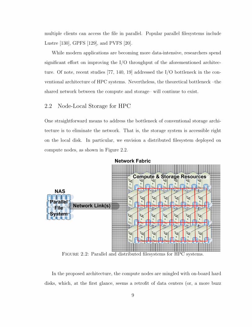
2.2 Node-Local Storage for HPC

One straightforward means to address the bottleneck of conventional storage archi-

tecture is to eliminate the network. That is, the storage system is accessible right

on the local disk. In particular, we envision a distributed filesystem deployed on

compute nodes, as shown in Figure 2.2.

Figure 2.2: Parallel and distributed filesystems for HPC systems.

In the proposed architecture, the compute nodes are mingled with on-board hard

disks, which, at the first glance, seems a retrofit of data centers (or, a more buzz

9

word cloud computing). But there are some key differences between HPC and cloud

computing. We list three of them in the following:

First, the interconnect within compute clusters is significant faster than data

centers. It is not uncommon to see 3D-torus network in HPC systems, whereas data

centers typically have Ethernet as their network infrastructure.

Second, the software stacks of HPC and data centers are different. Data centers

take good advantage of virtual machines for better system utilization, support popu-

lar high-level programming language such as Java, and so on. In contrast, HPC just

cannot sacrifice performance to improve utilization, since the top mission of HPC

systems are to accelerate large-scale simulations and experiments. More “modern”

programming language such as Java and Python, are not well supported because

most scientific applications are written in C and Fortran.

Last, and probably the most important, HPC and data centers target at different

users and workloads. As a case in point, the Hadoop filesystem (HDFS [134]) in data

centers deals with files of default 64MB chunks (preferable 128MB). This is because

in data centers files are typically large in size. HPC applications, however, have many

small- and medium-sized files, as Welch and Noer [151] reported that 25% – 90% of

all the 600 million files from 65 Panasas [99] installations are 64KB or smaller.

With all the above discrepancies among others, existing storage solutions in data

centers are not optimized for HPC machines. Therefore a distributed filesystem

crafted for HPC is in need. Nevertheless, before building a real distributed filesystems

on HPC compute nodes, we need simulations to justify our theoretical expectation,

and as co-design of the implementation.

2.3 Modeling HPC Storage Architecture

This section describes how we model the two major storage designs for large scale

HPC systems: remote parallel filesystems and node-local distributed filesystems. In

10

particular, we are interested in their checkpointing performance, one of the most

I/O-intensive applications in HPC. Before that, we introduce some metrics and ter-

minology.

Application Efficiency is defined as the ratio of application up time over the

total running time:

E “up time

running timeˆ 100%,

where running time is the summation of up time, checkpointing time, lost time and

rebooting time. Up time is when the job is correctly running on the computer.

Checkpointing time is when the system stores the correct states on persistent

storage periodically. Lost time measures the time when a failure occurred, the work

since the last checkpointing would be lost and needs to be recalculated. Rebooting

time is simply the time for the system to reboot the node.

Optimal Checkpointing Interval is the optimal checkpointing interval as mod-

eled in [26]:

OPT “a

2δpM `Rq ´ δ,

where δ is the checkpointing time, M is the system mean-time-to-failure (MTTF)

and R is the rebooting time of a job.

Memory Per Node is modeled as the following based on the specifications of

IBM BlueGene/P. When the system has fewer than 64K nodes, each node has 2GB

memory. For larger systems, the per-node memory is calculated (in GB) as

2 ¨#nodes

64K.

We have two different models of Storage Bandwidth for parallel filesystems

(PFS) and distributed filesystems (DFS), respectively, since they have completely

different architectures. We assume PFS is the state-of-the-art parallel filesystem used

11

in production today, e.g. GPFS [129], whose bandwidth (in GB/sec) is modeled as

BWPFS “#nodes

1000.

And for DFS, it is a hypothetical new storage architecture for exascale. There are no

real implementations of a DFS that can scale to exascale, but this study should be

a good motivator towards investing resources to the realization of DFS at exascale.

The bandwidth of DFS in our simulation has the following bandwidth

BWDFS “ #nodes ¨ plog #nodesq2.

These equations are based on our empirical observations on the IBM Blue Gene/P

supercomputer.

For rebooting time, DFS has a constant time of 85 seconds because each node is

independent to other nodes. For PFS, the rebooting time (in seconds) is calculated

as the following:

r0.0254 ¨#nodes` 55.296s,

which is also based on the empirical data of the IBM Blue Gene/P supercomputer.

The above formulae indicate that DFS has a linear scalability of checkpointing band-

width, whereas PFS only scales sub-linearly. The sub-linearity of PFS checkpoint

bandwidth would prevent it from working effectively for exascale systems.

2.4 The RXSim Simulator

For any job running on an HPC system, RXSim has three states: running, repairing,

restarting, as shown in Figure 2.3. This transmission works as follows: 1) when

a job is running, repairing or restarting, if a failure occurs then the job will be

hanged and enters repairing state; 2) after repaired, the job will restart, i.e. reboot

nodes occupied by this job; 3) after the job completes, it restarts its nodes; 4) after

12

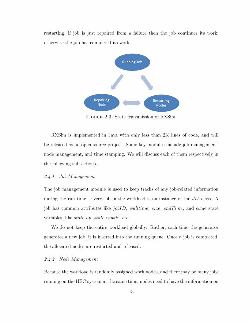
restarting, if job is just repaired from a failure then the job continues its work;

otherwise the job has completed its work.

Figure 2.3: State transmission of RXSim.

RXSim is implemented in Java with only less than 2K lines of code, and will

be released as an open source project. Some key modules include job management,

node management, and time stamping. We will discuss each of them respectively in

the following subsections.

2.4.1 Job Management

The job management module is used to keep tracks of any job-related information

during the run time. Every job in the workload is an instance of the Job class. A

job has common attributes like jobID, walltime, size, endT ime, and some state

variables, like state up, state repair, etc.

We do not keep the entire workload globally. Rather, each time the generator

generates a new job, it is inserted into the running queue. Once a job is completed,

the allocated nodes are restarted and released.

2.4.2 Node Management

Because the workload is randomly assigned work nodes, and there may be many jobs

running on the HEC system at the same time, nodes need to have the information on

13

which jobs are running on them. This is implemented by adding a jobID attribute to

the Node class. Nodes management is analogous to traditional memory management.

An array is fulfilled with instances of Node class, to keep all information e.g.

node ID, working state, etc. A free list is to keep and track all idle parts of the

HEC system, so that each time a job requests some computing resources (nodes),

RXSim will first check if there are enough idle nodes left. If so, RXSim retrieves

the first idle part of the HEC system and keeps doing so till the job gets enough

nodes. After a job is completed, the nodes occupied by this job will not be released

immediately. These nodes would be occupied by the completed job until they are

successfully rebooted.

2.4.3 Time Stamping

TimeStamp class is the event class where each timeStamp instance is an event with

some information related to time stamping. For example, if simulator encounters a

failure at some point, it creates a timeStamp instance including the incident’s time,

type, node ID, job ID.

There are four types of TimeStamp:

• Job ends successfully: with time and job ID.

• Job recovers: with time and job ID.

• Node reboots successfully: with time and job ID.

• Node failure: with time and node ID.

The TimeStamp queue is implemented as a TreeSet. The benefit of TreeSet is

that it will automatically sort the data, so it is easy to retrieve the latest event

from this queue. An obvious drawback of TreeSet is that its elements are hard to

be modified. Unfortunately modification is a frequent operation since the simulator

14

needs to update events in a regular basis. To fix the problem, we maintain another list

called uselessEventList, which keeps tracks of all idle TimeStamp. The simulator

would simply skip such an idle TimeStamp and try to retrieve the next available one.

2.5 Simulation Results

Experiments can be categorized into three major types. We first compare RXSim

results to existing valid results with the same parameters and workload to verify

RXSim. Then variant workloads are dispatched on RXSim to study the effectiveness

and efficiency of checkpointing at different scales of HEC systems. Lastly, we apply

RXSim on a 8-month log of an IBM Blue Gene/P supercomputer, and emulate

the checkpointing at exascale. Metrics Uptime, Check, Boot and Lost refer to the

definitions of up time, checkpointing time, rebooting time and lost time,

respectively, defined in Section 2.3

2.5.1 Experiment Setup

The single-node MTTF is set to 1000 years, optimistically, as claimed by IBM.

We assume it takes 0 second (again, very optimistically) to repair a single node.

Simulation time is set to 5 years, where each time step is 1 second.

2.5.2 Validation

Raicu et. al. [118] show how the applications look like for 3 cases: No-Checkpointing,

PFS with checkpointing, and DFS with checkpointing, as shown in Figure 2.4.

The result of RXSim with the same workload of Figure 2.4 is shown in Figure 2.5.

RXSim result is quite close to the published results: two lines have negligible differ-

ence, which is only due to the random variables used in the simulator.

Figure 2.6 shows the system reliability with checkpointing disabled. As we can

see, the system is basically not functioning beyond 400K nodes.

15

Figure 2.4: Comparison between checkpointings on different filesystems [118].

Figure 2.5: Comparison between RXSim and [118]

Figure 2.7 shows the system reliability when enabling checkpointing on a PFS.

We observe that the system up time is much longer than Figure 2.6. This is expected,

since checkpointing proves to be an effective mechanism to improve system reliability.

However, the efficiency is quite low (ă 10%) at exascale (1 million nodes), meaning

that PFS is not a good choice for checkpointing.

In Figure 2.8, we show the trends of system MTTF, the overhead of doing a

16

Figure 2.6: A no-checkpointing system stops functioning when having more than400K nodes.

Figure 2.7: System reliability when enabling checkpointing on a PFS: efficiency isquite low (ă 10%) at exascale (1 million nodes).

17

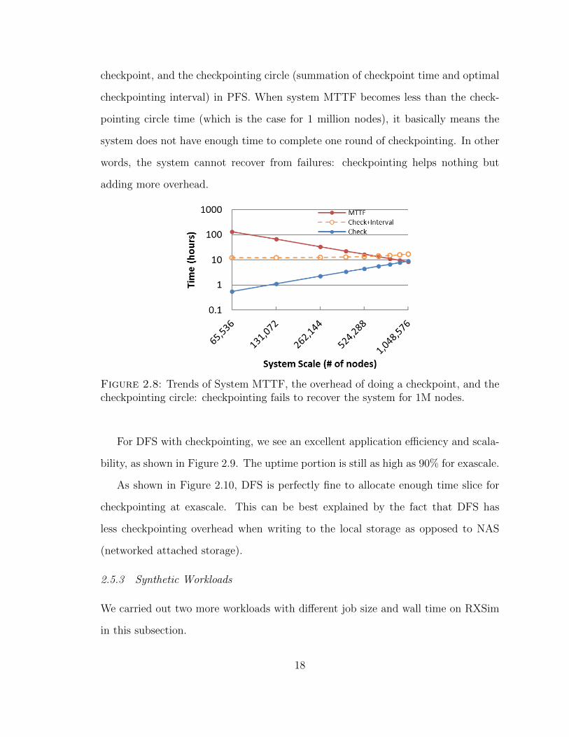
checkpoint, and the checkpointing circle (summation of checkpoint time and optimal

checkpointing interval) in PFS. When system MTTF becomes less than the check-

pointing circle time (which is the case for 1 million nodes), it basically means the

system does not have enough time to complete one round of checkpointing. In other

words, the system cannot recover from failures: checkpointing helps nothing but

adding more overhead.

Figure 2.8: Trends of System MTTF, the overhead of doing a checkpoint, and thecheckpointing circle: checkpointing fails to recover the system for 1M nodes.

For DFS with checkpointing, we see an excellent application efficiency and scala-

bility, as shown in Figure 2.9. The uptime portion is still as high as 90% for exascale.

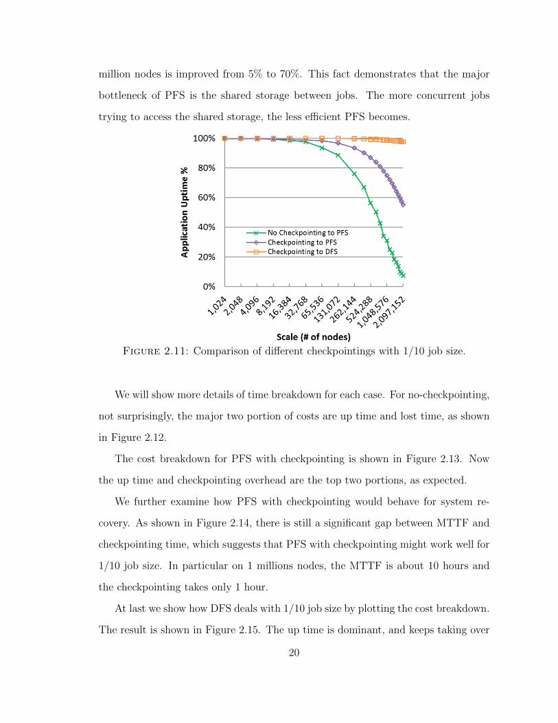
As shown in Figure 2.10, DFS is perfectly fine to allocate enough time slice for

checkpointing at exascale. This can be best explained by the fact that DFS has

less checkpointing overhead when writing to the local storage as opposed to NAS

(networked attached storage).

2.5.3 Synthetic Workloads

We carried out two more workloads with different job size and wall time on RXSim

in this subsection.

18

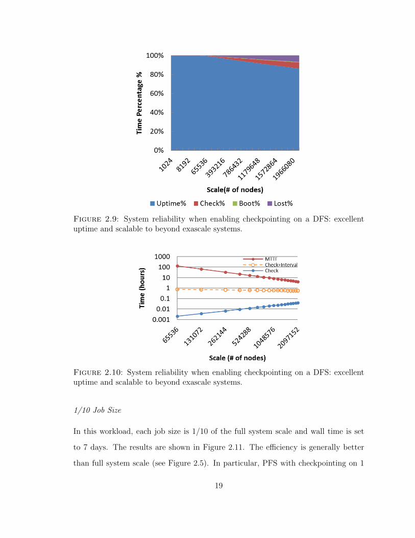
Figure 2.9: System reliability when enabling checkpointing on a DFS: excellentuptime and scalable to beyond exascale systems.

Figure 2.10: System reliability when enabling checkpointing on a DFS: excellentuptime and scalable to beyond exascale systems.

1/10 Job Size

In this workload, each job size is 1/10 of the full system scale and wall time is set

to 7 days. The results are shown in Figure 2.11. The efficiency is generally better

than full system scale (see Figure 2.5). In particular, PFS with checkpointing on 1

19

million nodes is improved from 5% to 70%. This fact demonstrates that the major

bottleneck of PFS is the shared storage between jobs. The more concurrent jobs

trying to access the shared storage, the less efficient PFS becomes.

Figure 2.11: Comparison of different checkpointings with 1/10 job size.

We will show more details of time breakdown for each case. For no-checkpointing,

not surprisingly, the major two portion of costs are up time and lost time, as shown

in Figure 2.12.

The cost breakdown for PFS with checkpointing is shown in Figure 2.13. Now

the up time and checkpointing overhead are the top two portions, as expected.

We further examine how PFS with checkpointing would behave for system re-

covery. As shown in Figure 2.14, there is still a significant gap between MTTF and

checkpointing time, which suggests that PFS with checkpointing might work well for

1/10 job size. In particular on 1 millions nodes, the MTTF is about 10 hours and

the checkpointing takes only 1 hour.

At last we show how DFS deals with 1/10 job size by plotting the cost breakdown.

The result is shown in Figure 2.15. The up time is dominant, and keeps taking over

20

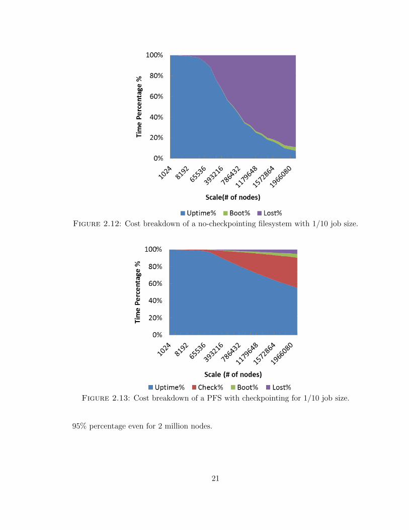
Figure 2.12: Cost breakdown of a no-checkpointing filesystem with 1/10 job size.

Figure 2.13: Cost breakdown of a PFS with checkpointing for 1/10 job size.

95% percentage even for 2 million nodes.

21

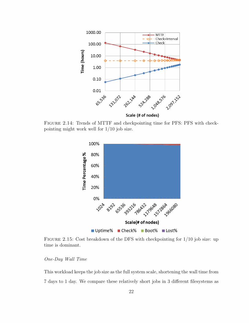
Figure 2.14: Trends of MTTF and checkpointing time for PFS: PFS with check-pointing might work well for 1/10 job size.

Figure 2.15: Cost breakdown of the DFS with checkpointing for 1/10 job size: uptime is dominant.

One-Day Wall Time

This workload keeps the job size as the full system scale, shortening the wall time from

7 days to 1 day. We compare these relatively short jobs in 3 different filesystems as

22

shown in Figure 2.16. Again, DFS outperforms other two and keeps high efficiency

of 90% on 1 million nodes. However, PFS is degenerated to be worse than no-

checkpointing.

Figure 2.16: Efficiency of different checkpointing scenarios for short jobs: DFSworks fine, but PFS with checkpointing does not help improve up time.

We show the cost breakdown of PFS and no-checkpointing in Figure 2.17 and Fig-

ure 2.18 respectively, in order to investigate why PFS has such poor performance.

The cost distributions of both cases are about the same, except for PFS has some

additional time spent on checkpointing which only takes a small portion (ă 10%).

The reason is most likely that the wall time of each job was much shorter, which

implies less lost-time during a failure. The checkpointing interval and checkpoint-

ing overhead are quite sensitive to wall time, therefore shortening jobs dramatically

hurts the application efficiency of PFS with checkpointing. The implication, in or-

der, is that, for short jobs no-checkpointing might do as equally well as PFS with

checkpointing enabled.

2.5.4 Real Logs of IBM Blue Gene/P

We carried out experiments on real workloads (8-month log) from IBM Blue Gene/P

supercomputer (a.k.a. Intrepid) at Argonne National Laboratory (ANL). Intrepid

23

Figure 2.17: Cost breakdown of no-checkpointing filesystem for 1-day jobs.

Figure 2.18: Cost breakdown of PFS with checkpointing for 1-day jobs.

has a peak of 557TFlops, has 40 racks, and comprises 40960 quad-core nodes (163840

cores in total), associated I/O nodes, storage servers (NAS), and high bandwidth

24

torus network interconnecting compute nodes. It debuted as No.3 in the top 500

supercomputer list released in June 2008.

The log in the experiment contains 8 months of accounting records of Intrepid.

The log data is in swf (standard workload format). We scaled the job size on the

log in proportion to scale RXSim from 1024 to 2 million nodes. Note that the data

beyond 40K nodes are predicted by RXSim, since the Blue Gene/P only has 40K

nodes (160K cores).

Figure 2.19: Application efficiency for Blue Gene/P jobs.

Figure 2.19 shows that a no-checkpointing filesystem outperforms PFS with

checkpointing, which is counter intuitive at the first glance. The reason is that

the Blue Gene/P jobs have an average wall time of 5k seconds, which is less than 2

hours and far shorter than 1 day in Figure 2.16. So this result in fact justifies our

previous conclusion that short jobs would badly hurt the application efficiency by

enabling checkpointing.

We show the cost breakdown of different filesystems in Figure 2.20. PFS has a

significant portion of checkpointing overhead, booting time and lost-time in exascale

25

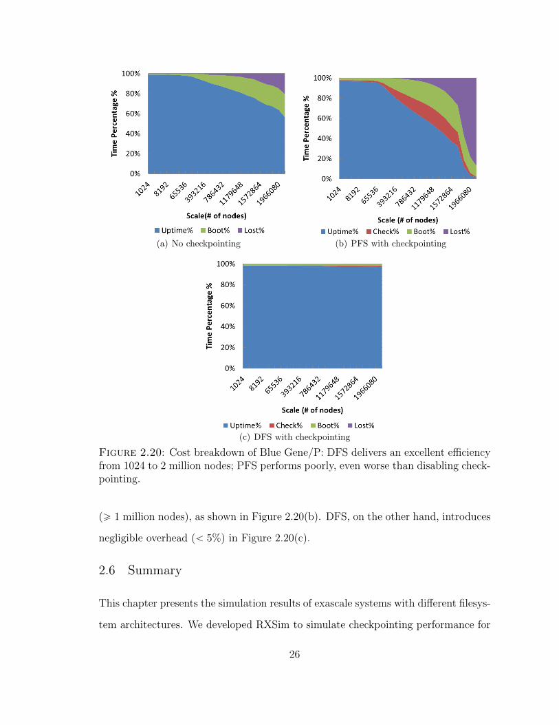
(a) No checkpointing (b) PFS with checkpointing

(c) DFS with checkpointing

Figure 2.20: Cost breakdown of Blue Gene/P: DFS delivers an excellent efficiencyfrom 1024 to 2 million nodes; PFS performs poorly, even worse than disabling check-pointing.

(ě 1 million nodes), as shown in Figure 2.20(b). DFS, on the other hand, introduces

negligible overhead (ă 5%) in Figure 2.20(c).

2.6 Summary

This chapter presents the simulation results of exascale systems with different filesys-

tem architectures. We developed RXSim to simulate checkpointing performance for

26

exascale computing. RXSim suggests distributed filesystems are more optimistic

than state-of-the-art parallel filesystems for reliable exascale computers. In particu-

lar, we found that local persistent storage would be dramatically helpful to leverage

data locality in the context of traditional distributed filesystems. Our study shows

that local storage would be one of the key points to succeed in maintaining the re-

liability for exascale computers. The results are coincident with the findings in [30],

where a hybrid of local/global checkpointing mechanism was proposed for the pro-

jected exascale system.

27

3

FusionFS: the Fusion Distributed Filesystem

State-of-the-art yet decades old architecture of high performance computing (HPC)

systems has its compute and storage resources separated. It has shown limits for to-

day’s data-intensive scientific applications, because every I/O needs to be transferred

via the network between the compute and storage cliques. This chapter describes a

distributed storage layer local to the compute nodes, which is responsible for most

of the I/O operations and saves extreme amount of data movement between com-

pute and storage resources. We have designed and implemented a system prototype

of such architecture –the FusionFS distributed filesystem– to support metadata-

intensive and write-intensive operations, both of which are critical to the I/O perfor-

mance of scientific applications. FusionFS has been deployed and evaluated on up to

16K compute nodes in an IBM Blue Gene/P supercomputer, showing more than an

order of magnitude performance improvement over other popular file systems such

as GPFS, PVFS, and HDFS.

28

3.1 Background

The conventional architecture of high-performance computing (HPC) systems sep-

arates the compute and storage resources into two cliques (i.e. compute nodes and

storage nodes), both of which are interconnected by a shared network infrastructure.

This architecture is mainly a result from the nature of many legacy large-scale sci-

entific applications that are compute intensive, where it is often assumed that the

storage I/O capabilities are lightly utilized for the initial data input, some periodic

checkpoints, and the final output. However, in the era of Big Data, scientific ap-

plications are becoming more and more data-intensive, requiring a greater degree of

support from the storage subsystem [38].

While recent studies [77, 140] addressed the I/O bottleneck in the conventional

architecture of HPC systems, this paper is orthogonal to them by proposing a new

storage architecture to co-locate the storage and compute resources. In particular,

we envision a distributed storage system on compute nodes for applications to manip-

ulate their intermediate results and checkpoints, rather than transferring data over

the network. While co-location of storage and computation has been widely lever-

aged in data centers (e.g. Hadoop clusters), such architecture never exists in HPC

systems. This work, to the best of our knowledge, for the first time demonstrates

how to architect and engineer such a system, and reports how much, quantitatively,

it could improve the I/O performance of real scientific applications.

The proposed architecture of co-locating compute and storage could raise con-

cerns about jitters on compute nodes, since applications’ computation and I/O share

resources like CPU and network. We argue that the I/O-related cost can be offloaded

onto dedicated infrastructures that are decoupled from the application’s acquired re-

sources, as justified in [31]. In fact, this resource-isolation strategy has been applied

in production systems: the IBM Blue Gene/Q supercomputer (Mira [92]) assigns one

29

core of the chip (17 cores in total) for the local operating system and the other 16

cores for applications.

Distributed storage has been extensively studied in data centers (e.g. the popular

distributed file system HDFS [134]); yet there exists little literature for building a

distributed storage system particularly for HPC systems whose design principles are

much different from data centers. HPC nodes are highly customized and tightly

coupled with high throughput and low latency network (e.g. InfiniBand), while data

centers typically have commodity servers and inexpensive networks (e.g. Ethernet).

So storage systems designed for data centers are not optimized for the HPC machines,

as we will discuss in more detail where HDFS shows poor performance on a typical

HPC machine (Figure 3.12). In particular, we observe that the following challenges

are unique to a distributed file system on HPC compute nodes, related to both

metadata-intensive and write-intensive workloads:

(1) The storage system on HPC compute nodes needs to support intensive meta-

data operations. Many scientific applications create a large number of small- to

medium-sized files, as Welch and Noer [151] reported that 25% – 90% of all the 600

million files from 65 Panasas [99] installations are 64KB or smaller. So the I/O perfor-

mance is highly throttled by the metadata rate, besides the data itself. Data centers,

however, is not optimized for this type of workload. If we recall that HDFS [134]

splits a large file into a series of default 64MB chunks (128MB recommended in most

cases) for parallel processing, a small- or medium-sized file can benefit little from this

data parallelism. Moreover, the centralized metadata server in HDFS is apparently

not designed to handle intensive metadata operations.

(2) File writes should be optimized for a distributed file system on HPC com-

pute nodes. The fault tolerance of most today’s large-scale HPC systems is achieved

through some form of checkpointing. In essence, the system periodically flushes mem-

ory to external persistent storage, and occasionally loads the data back to memory

30

to roll back to the most recent correct checkpoint up on a failure. So file writes

typically outnumber file reads in terms of both frequency and size in HPC systems,

and improving the write performance will significantly reduce the overall I/O cost.

The fault tolerance of data centers, however, is not achieved through checkpointing

its memory states, but the re-computation of affected data chunks that are replicated

on multiple nodes.

3.2 Design Overview

As shown in Figure 3.1, FusionFS [182, 172] is a user-level file system that runs on

the compute resource infrastructure, and enables every compute node to actively

participate in both the metadata and data movement. The client (or application) is

able to access the global namespace of the file system with a distributed metadata

service. Metadata and data are completely decoupled: the metadata on a particular

compute node does not necessarily describe the data residing on the same compute

node. The decoupling of metadata and data allows different strategies to be applied

to metadata and data management, respectively.

FusionFS supports both the POSIX interface and a user library. The POSIX

interface is implemented with the FUSE framework [40], so that legacy applications

can run directly on FusionFS without modifications. Just like other user-level file

systems (e.g. PVFS [20]), FusionFS can be deployed as a mount point in a UNIX-

like system. The mount point is a virtual root directory to the clients when using

FusionFS.

Users need to specify three arguments when deploying FusionFS as a POSIX-

compliant mount point on a compute node: the scratch directory where to store

the metadata and data, the mount point of the remote parallel file system (e.g.

Lustrue [130], GPFS [129], PVFS [20]), and the mount point of FusionFS where

applications manipulate files. The remote parallel file system needs to be integral to

31

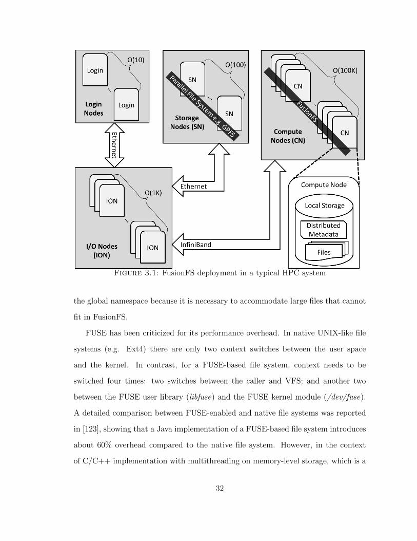
Figure 3.1: FusionFS deployment in a typical HPC system

the global namespace because it is necessary to accommodate large files that cannot

fit in FusionFS.

FUSE has been criticized for its performance overhead. In native UNIX-like file

systems (e.g. Ext4) there are only two context switches between the user space

and the kernel. In contrast, for a FUSE-based file system, context needs to be

switched four times: two switches between the caller and VFS; and another two

between the FUSE user library (libfuse) and the FUSE kernel module (/dev/fuse).

A detailed comparison between FUSE-enabled and native file systems was reported

in [123], showing that a Java implementation of a FUSE-based file system introduces

about 60% overhead compared to the native file system. However, in the context

of C/C++ implementation with multithreading on memory-level storage, which is a

32

typical setup in HPC systems, the overhead is much lower. In prior work [174], we

reported that FUSE could deliver as high as 578MB/s throughput, 85% of the raw

bandwidth.

To avoid the performance overhead from FUSE, FusionFS also provides a user

library for applications to directly interact with their files. These APIs look similar

to POSIX, for example ffs open(), ffs close(), ffs read(), and ffs write(). The down-

side of this approach is the lack of POSIX support, indicating that the application

might not be portable to other file systems, and often needs some modifications and

recompilation.

3.3 Metadata Management

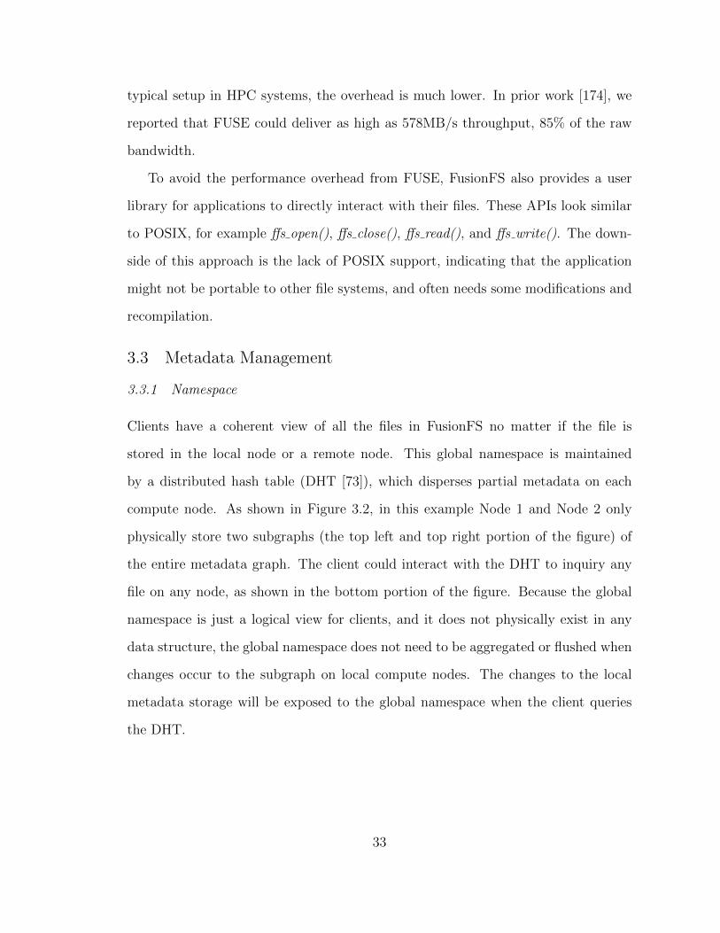
3.3.1 Namespace

Clients have a coherent view of all the files in FusionFS no matter if the file is

stored in the local node or a remote node. This global namespace is maintained

by a distributed hash table (DHT [73]), which disperses partial metadata on each

compute node. As shown in Figure 3.2, in this example Node 1 and Node 2 only

physically store two subgraphs (the top left and top right portion of the figure) of

the entire metadata graph. The client could interact with the DHT to inquiry any

file on any node, as shown in the bottom portion of the figure. Because the global

namespace is just a logical view for clients, and it does not physically exist in any

data structure, the global namespace does not need to be aggregated or flushed when

changes occur to the subgraph on local compute nodes. The changes to the local

metadata storage will be exposed to the global namespace when the client queries

the DHT.

33

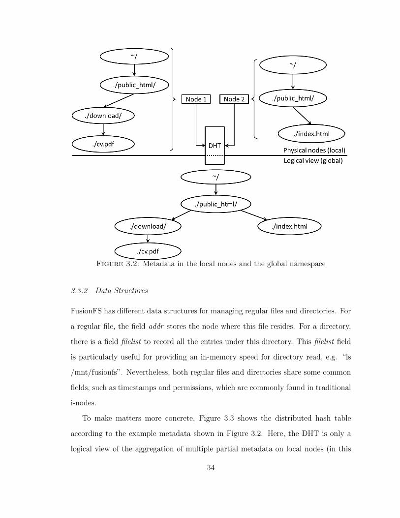
Figure 3.2: Metadata in the local nodes and the global namespace

3.3.2 Data Structures

FusionFS has different data structures for managing regular files and directories. For

a regular file, the field addr stores the node where this file resides. For a directory,

there is a field filelist to record all the entries under this directory. This filelist field

is particularly useful for providing an in-memory speed for directory read, e.g. “ls

/mnt/fusionfs”. Nevertheless, both regular files and directories share some common

fields, such as timestamps and permissions, which are commonly found in traditional

i-nodes.

To make matters more concrete, Figure 3.3 shows the distributed hash table

according to the example metadata shown in Figure 3.2. Here, the DHT is only a

logical view of the aggregation of multiple partial metadata on local nodes (in this

34

case, Node 1 and Node 2). Five entries (three directories, two regular files) are stored

in the DHT, with their file names as keys. The value is a list of properties delimited

by semicolons. For example, the first and second portions of the values are permission

flag and file size, respectively. The third portion for a directory value is a list of its

entries delimited by commas, while for regular files it is just the physical location of

the file, e.g. the IP address of the node on which the file is stored. The value in the

figure as a string delimited by semicolons is, in fact, only for clear representation.

In implementation, the value is stored in a C structure. Upon a client request, this

value structure is serialized by Google Protocol Buffers [114] before sending over

the network to the metadata server, which is just another compute node. Similarly,

when the metadata blob is received by a node, we deserialize the blob back into the

C structure with Google Protocol Buffers.

Figure 3.3: The global namespace abstracted by key-value pairs in a DHT

The metadata and data on a local node are completely decoupled: a regular

35

file’s location is independent of its metadata location. From Figure 3.2, we know

the index.html metadata is stored on Node 2, and the cv.pdf metadata is on Node

1. However, it is perfectly fine for index.html to reside on Node 1, and for cv.pdf

to reside on Node 2, as shown in Figure 3.3. Besides the conventional metadata

information for regular files, there is a special flag in the value indicating if this file

is being written. Specifically, any client who requests to write a file needs to sets this

flag before opening the file, and will not reset it until the file is closed. The atomic

compare-swap operation supported by DHT [73] guarantees the file consistency for

concurrent writes.

Another challenge on the metadata implementation is on the large-directory per-

formance issues. In particular, when a large number of clients write many small files

on the same directory concurrently, the value of this directory in the key-value pair

gets incredibly long and responds extremely slow. The reason is that a client needs to

update the entire old long string with the new one, even though the majority of the

old string is unchanged. To fix that, we implement an atomic append operation that

asynchronously appends the incremental change to the value. This approach is simi-

lar to Google File System [44], where files are immutable and can only be appended.

This gives us excellent concurrent metadata modification in large directories, at the

expense of potentially slower directory metadata read operations.

3.3.3 Network Protocols

We encapsulate several network protocols in an abstraction layer. Users can specify

which protocol to be applied in their deployments. Currently, we support three

protocols: TCP, UDP, and MPI. Since we expect a high network concurrency on

metadata servers, epoll is used instead of multithreading. The side effect of epoll is

that the received message packets are not kept in the same order as on the sender. To

address this, a header [message id, packet id] is added to the message at the sender,

36

and the message is restored by sorting the packet id for each message at the recipient.

This is efficiently done by a sorted map with message id as the key, mapping to a

sorted set of the message’s packets.

3.3.4 Persistence

The whole point of the proposed distributed metadata architecture is to improve

performance. Thus, any metadata manipulation from clients should occur in memory,

plus some network transfer if needed. On the other hand, persistence is required for

metadata just in case of any memory errors or system restarts.

The persistence of metadata is achieved by periodically flushing the in-memory

metadata onto the local persistent storage. In some sense, it is similar to the incre-

mental checkpointing mechanism. This asynchronous flushing helps to sustain the

high performance of the in-memory metadata operations.

3.3.5 Fault Tolerance

When a node fails, we need to restore the missing metadata and files on that node as

soon as possible. The traditional method for data replication is to make a number

of replicas to the primary copy. When the primary copy is failed, one of the replicas

will be restored to replace the failed primary copy. This method has its advantages

such as ease-of-use, less compute-intensive, when compared to the emerging erasure-

coding mechanism [111, 126]. The main critique on replicas is, however, its low

storage efficiency. For example, in Google file system [44] each primary copy has two

replicas, which results in the storage utilization as 11`2

“ 33%.

For fault tolerance of metadata, we chose data replication for metadata based on

the following observations. First, metadata size is typically much smaller than file

data in orders of magnitude. Therefore, replicating the metadata impact little to

the overall space utilization of the entire system. Second, the computation overhead

37

introduced by erasure coding can hardly be amortized by the reduced I/O time on

transferring the encoded metadata. In essence, erasure coding is preferred when data

is large and the time needed to encode and decode files would be offset by the benefit

of sending less data to remote nodes (i.e. less network consumption). This is not

the case for transferring metadata, where the primary metric is latency (and not

bandwidth).

3.3.6 Consistency

Since each primary metadata copy has replicas, the next questions is how make

them consistent. Traditionally, there are two semantics to keep replicas consistent:

(1) strong consistent – blocking until replicas are finished with updating; (2) weak

consistent – return immediately when the primary copy is updated. The tradeoff be-

tween performance and consistency is tricky, most likely depending on the workload

characteristics.

As for a system design without any a priori information on the particular work-

load, we compromise with both sides: assuming the replicas are ordered by some

criteria (e.g. last modification time), the first replica is strong consistent to the

primary copy, and the other replicas are updated asynchronously. By doing this,

the metadata are strong consistent (in the average case) while the overhead is kept

relatively low.

3.4 Data Movement Protocols

3.4.1 Network Transfer

For file transfer, neither UDP nor TCP is ideal for FusionFS on HPC compute nodes.

UDP is a highly efficient protocol, but is lack of reliability support. TCP, on the

other hand, supports reliable transfer of packets, but adds significant overhead.

We have developed our own data transfer service Fusion Data Transfer (FDT)

38

on top of UDP-based Data Transfer (UDT) [48]. UDT is a reliable UDP-based

application level data transport protocol for distributed data-intensive applications.

UDT adds its own reliability and congestion control on top of UDP that offers a

higher speed than TCP.

3.4.2 File Open

Figure 3.4 shows the protocol when opening a file in FusionFS. Due to limited space,

we assume the requested file is also on Node-j. Note that it is not necessarily Node-j

who stores both the requested file and its metadata, as we explained in §3.3.2 that

the metadata and data are decoupled on compute nodes.

Figure 3.4: The protocol of file open in FusionFS

In step 1, the application on Node-i issues a POSIX fopen() call that is caught

by the implementation in the FUSE user-level interface (i.e. libfuse) for file open.

Steps 2 – 5 retrieve the file location from the metadata service that is implemented

by a distributed hash table [73]. The location information might be stored in another

39

machine Node-j, so this procedure could involve a round trip of messages between

Node-i and Node-j. Then Node-i needs to ping Node-j to fetch the file in steps 6 – 7.

Step 8 triggers the system call to open the transferred file and finally step 9 returns

the file handle to the application.

3.4.3 File Write

Before writing to a file, the process checks if the file is being accessed by another

process, as discussed in §3.3.2. If so, an error number is returned to the caller.

Otherwise the process can do one of the following two things. If the file is originally

stored on a remote node, the file is transferred to the local node in the fopen()

procedure, after which the process writes to the local copy. If the file to be written

is right on the local node, or it is a new file, then the process starts writing the file

just like a system call.

The aggregate write throughput is obviously optimal because file writes are as-

sociated with local I/O throughput and avoids the following two types of cost: (1)

the procedure to determine to which node the data will be written, normally ac-

complished by pinging the metadata nodes or some monitoring services, and (2)

transferring the data to a remote node. The downside of this file write strategy is

the poor control on the load balance of compute node storage. This issue could be

addressed by an asynchronous re-balance procedure running in the background, or

by a load-aware task scheduler that steals tasks from the active nodes to the more

idle ones.

When the process finishes writing to a file that is originally stored in another

node, FusionFS does not send the newly modified file back to its original node.

Instead, the metadata of this file is updated. This saves the cost of transferring the

file data over the network.

40

3.4.4 File Read

Unlike file write, it is impossible to arbitrarily control where the requested data

reside for file read. The location of the requested data is highly dependent on the

I/O pattern. However, we could determine which node the job is executed on by the

distributed workflow system, e.g. Swift [183]. That is, when a job on node A needs

to read some data on node B, we reschedule the job on node B. The overhead of

rescheduling the job is typically smaller than transferring the data over the network,

especially for data-intensive applications. In our previous work [119], we detailed this

approach, and justified it with theoretical analysis and experiments on benchmarks

and real applications.

Indeed, remote readings are not always avoidable for some I/O patterns, e.g.

merge sort. In merge sort, the data need to be joined together, and shifting the job

cannot avoid the aggregation. In such cases, we need to transfer the requested data

from the remote node to the requesting node. The data movement across compute

nodes within FusionFS is conducted by the FDT service discussed in §3.4.1. FDT

service is deployed on each compute node, and keeps listening to the incoming fetch

and send requests.

3.4.5 File Close

Figure 3.5 shows the protocol when closing a file in FusionFS. In steps 1 – 3 the

application on Node-i closes and flushes the file to the local disk. If this is a read-

only operation before the file is closed, then libfuse only needs to signal the caller

(i.e. the application) in step 10. If this file has been modified, then its metadata

needs to be updated in steps 4 – 7. Moreover, the replicas of this file also need to be

updated in steps 8 – 9.

Again, just like Figure 3.4, the replica is not necessarily stored on the same node

of its metadata (Node-j).

41

Figure 3.5: The protocol of file close in FusionFS

3.5 Experiment Results

While we indeed compare FusionFS to some open-source systems such as PVFS [20]

(in Figure 3.8) and HDFS [134] (in Figure 3.12), our top mission is to evaluate its

performance improvement over the production file system of today’s fastest systems.

If we look at today’s top 10 supercomputers [143], 4 systems are IBM Blue Gene/Q

systems which run GPFS [129] as the default file system. Therefore most large-scale

experiments conducted in this paper are carried out on Intrepid [58], a 40K-node

IBM Blue Gene/P supercomputer whose default file system is also GPFS.

Intrepid serves as a test bed for FusionFS more as a demonstration of the scal-

ability we plan to achieve in a hypothetical deployment with many compute nodes

and node-local storage. Note that FusionFS is not a customized file system only for

42

Intrepid, but an implementation for HPC compute nodes in general.

Each Intrepid compute node has quad core 850MHz PowerPC 450 processors and

runs a light-weight Linux ZeptoOS [162] with 2 GB memory. A 7.6PB GPFS [129]

parallel file system is deployed on 128 storage nodes. When FusionFS is evaluated

as a POSIX-compliant file system, each compute node gets access to a local storage

mount point with 174 MB/s throughput on par with today’s high-end hard drives.

It points to the ramdisk and is throttled by a single-threaded FUSE layer. The

network protocols for metadata management and file manipulation are TCP and

FDT, respectively.

All experiments are repeated at least five times, or until results become stable

(within 5% margin of error). The reported numbers are the average of all runs.

Caching effect is carefully precluded by reading a file larger than the on-board mem-

ory before the measurement.

3.5.1 Metadata Rate

We expect that the metadata performance of FusionFS should be significantly higher

than the remote GPFS on Intrepid, because FusionFS manipulates metadata in a

completely distributed manner on compute nodes while GPFS has a limited number

of clients on I/O nodes (every 64 compute nodes share one I/O node in GPFS). To

quantitatively study the improvement, both FusionFS and GPFS create 10K empty

files from each client on its own directory on Intrepid. That is, at 1024-nodes scale,

we create 10M files over 1024 directories. We could have let all clients write on

the same directory, but this workload would not take advantage of GPFS’ multiple

I/O nodes. That is, we want to optimize GPFS’ performance when comparing it to

FusionFS.

As shown in Figure 3.6, at 1024-nodes scale, FusionFS delivers nearly two orders

of magnitude higher metadata rate over GPFS. FusionFS shows excellent scalability,

43

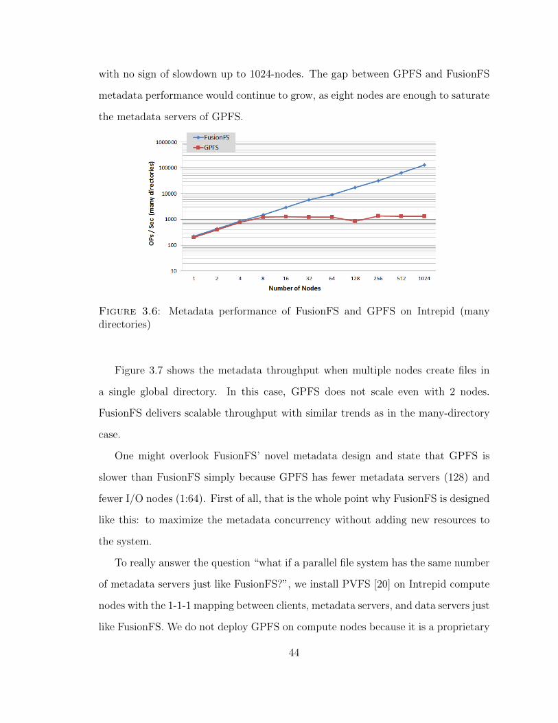
with no sign of slowdown up to 1024-nodes. The gap between GPFS and FusionFS

metadata performance would continue to grow, as eight nodes are enough to saturate

the metadata servers of GPFS.

Figure 3.6: Metadata performance of FusionFS and GPFS on Intrepid (manydirectories)

Figure 3.7 shows the metadata throughput when multiple nodes create files in

a single global directory. In this case, GPFS does not scale even with 2 nodes.

FusionFS delivers scalable throughput with similar trends as in the many-directory

case.

One might overlook FusionFS’ novel metadata design and state that GPFS is

slower than FusionFS simply because GPFS has fewer metadata servers (128) and

fewer I/O nodes (1:64). First of all, that is the whole point why FusionFS is designed

like this: to maximize the metadata concurrency without adding new resources to

the system.

To really answer the question “what if a parallel file system has the same number

of metadata servers just like FusionFS?”, we install PVFS [20] on Intrepid compute

nodes with the 1-1-1 mapping between clients, metadata servers, and data servers just

like FusionFS. We do not deploy GPFS on compute nodes because it is a proprietary

44

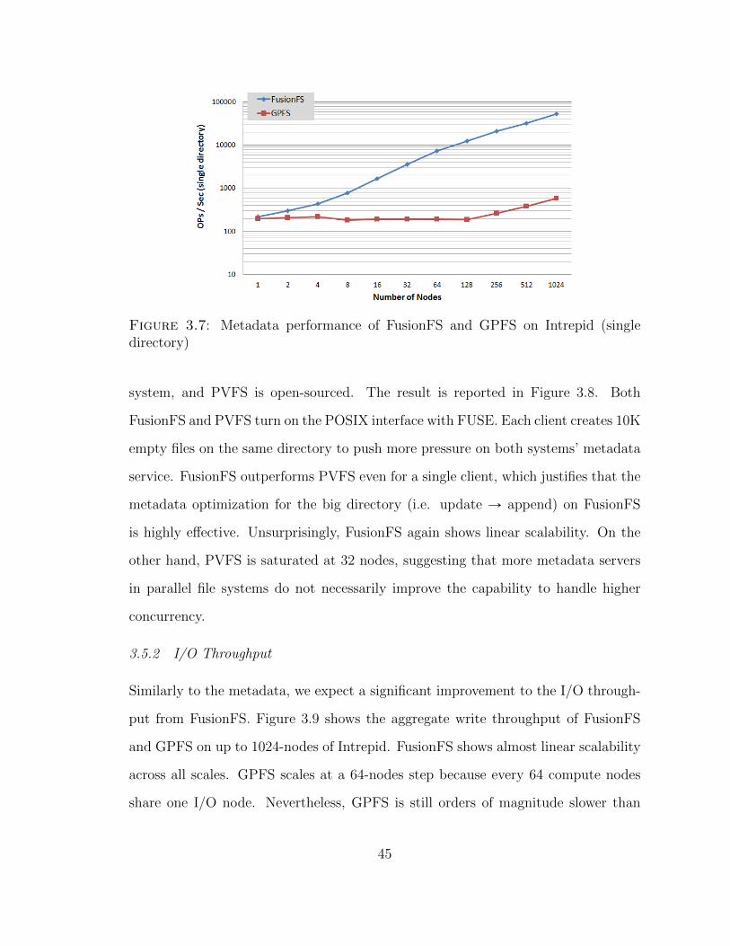
Figure 3.7: Metadata performance of FusionFS and GPFS on Intrepid (singledirectory)

system, and PVFS is open-sourced. The result is reported in Figure 3.8. Both

FusionFS and PVFS turn on the POSIX interface with FUSE. Each client creates 10K

empty files on the same directory to push more pressure on both systems’ metadata

service. FusionFS outperforms PVFS even for a single client, which justifies that the

metadata optimization for the big directory (i.e. update Ñ append) on FusionFS

is highly effective. Unsurprisingly, FusionFS again shows linear scalability. On the

other hand, PVFS is saturated at 32 nodes, suggesting that more metadata servers

in parallel file systems do not necessarily improve the capability to handle higher

concurrency.

3.5.2 I/O Throughput

Similarly to the metadata, we expect a significant improvement to the I/O through-

put from FusionFS. Figure 3.9 shows the aggregate write throughput of FusionFS

and GPFS on up to 1024-nodes of Intrepid. FusionFS shows almost linear scalability

across all scales. GPFS scales at a 64-nodes step because every 64 compute nodes

share one I/O node. Nevertheless, GPFS is still orders of magnitude slower than

45

Figure 3.8: Metadata performance of FusionFS and PVFS on Intrepid (singledirectory)

FusionFS at all scales. In particular, at 1024-nodes, FusionFS outperforms GPFS

with a 57X higher throughput (113 GB/s vs. 2 GB/s).

Figure 3.10 shows FusionFS’s scalability at extreme scales. The experiment is

carried out on Intrepid on up to 16K-node each of which has a FusionFS mount

point. FusionFS throughput shows about linear scalability: doubling the number of

nodes yield doubled throughput. Specifically, we observe stable 2.5 TB/s throughput

(peak 2.64 TB/s) on 16K-nodes.

The main reason why FusionFS data write is faster is that the compute node

only writes to its local storage. This is not true for data read though: it is possible

that one node needs to transfer some remote data to its local disk. Thus, we are

interested in two extreme scenarios (i.e. all-local read and all-remote read) that

define the lower and upper bounds of read throughput. We measure FusionFS for

both cases on 256-nodes of Intrepid, where each compute node reads a file of different

sizes from 1 MB to 256 MB. For the all-local case (e.g. where a data-aware scheduler

46

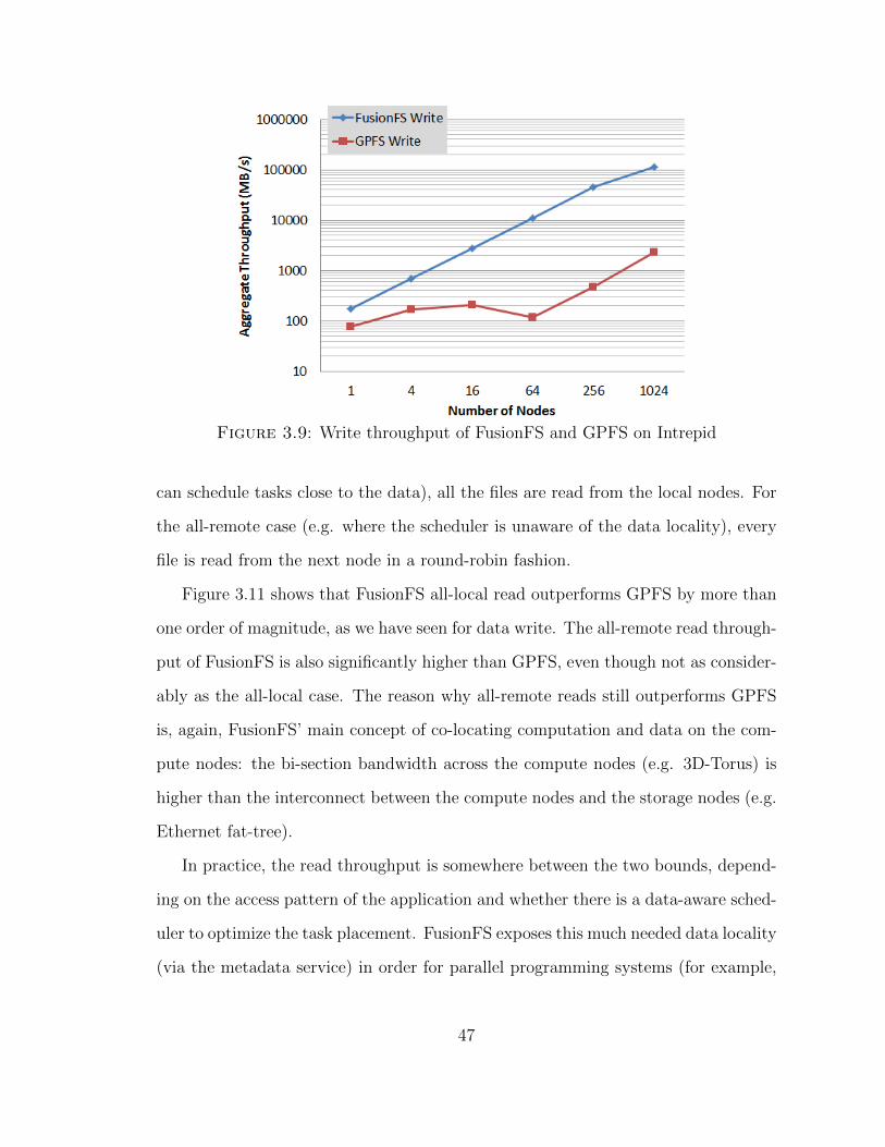
Figure 3.9: Write throughput of FusionFS and GPFS on Intrepid

can schedule tasks close to the data), all the files are read from the local nodes. For

the all-remote case (e.g. where the scheduler is unaware of the data locality), every

file is read from the next node in a round-robin fashion.

Figure 3.11 shows that FusionFS all-local read outperforms GPFS by more than

one order of magnitude, as we have seen for data write. The all-remote read through-

put of FusionFS is also significantly higher than GPFS, even though not as consider-

ably as the all-local case. The reason why all-remote reads still outperforms GPFS

is, again, FusionFS’ main concept of co-locating computation and data on the com-

pute nodes: the bi-section bandwidth across the compute nodes (e.g. 3D-Torus) is

higher than the interconnect between the compute nodes and the storage nodes (e.g.

Ethernet fat-tree).

In practice, the read throughput is somewhere between the two bounds, depend-

ing on the access pattern of the application and whether there is a data-aware sched-

uler to optimize the task placement. FusionFS exposes this much needed data locality

(via the metadata service) in order for parallel programming systems (for example,

47

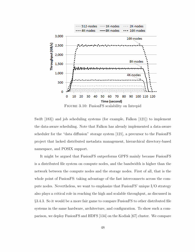
Figure 3.10: FusionFS scalability on Intrepid

Swift [183]) and job scheduling systems (for example, Falkon [121]) to implement

the data-aware scheduling. Note that Falkon has already implemented a data-aware

scheduler for the “data diffusion” storage system [121], a precursor to the FusionFS

project that lacked distributed metadata management, hierarchical directory-based

namespace, and POSIX support.

It might be argued that FusionFS outperforms GPFS mainly because FusionFS

is a distributed file system on compute nodes, and the bandwidth is higher than the

network between the compute nodes and the storage nodes. First of all, that is the

whole point of FusionFS: taking advantage of the fast interconnects across the com-

pute nodes. Nevertheless, we want to emphasize that FusionFS’ unique I/O strategy

also plays a critical role in reaching the high and scalable throughput, as discussed in

§3.4.3. So it would be a more fair game to compare FusionFS to other distributed file

systems in the same hardware, architecture, and configuration. To show such a com-

parison, we deploy FusionFS and HDFS [134] on the Kodiak [67] cluster. We compare

48

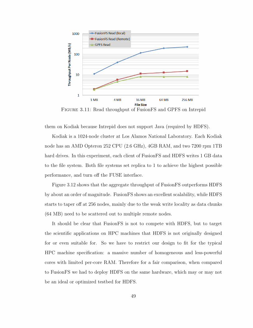
Figure 3.11: Read throughput of FusionFS and GPFS on Intrepid

them on Kodiak because Intrepid does not support Java (required by HDFS).

Kodiak is a 1024-node cluster at Los Alamos National Laboratory. Each Kodiak

node has an AMD Opteron 252 CPU (2.6 GHz), 4GB RAM, and two 7200 rpm 1TB

hard drives. In this experiment, each client of FusionFS and HDFS writes 1 GB data

to the file system. Both file systems set replica to 1 to achieve the highest possible

performance, and turn off the FUSE interface.

Figure 3.12 shows that the aggregate throughput of FusionFS outperforms HDFS

by about an order of magnitude. FusionFS shows an excellent scalability, while HDFS

starts to taper off at 256 nodes, mainly due to the weak write locality as data chunks

(64 MB) need to be scattered out to multiple remote nodes.

It should be clear that FusionFS is not to compete with HDFS, but to target

the scientific applications on HPC machines that HDFS is not originally designed

for or even suitable for. So we have to restrict our design to fit for the typical

HPC machine specification: a massive number of homogeneous and less-powerful

cores with limited per-core RAM. Therefore for a fair comparison, when compared

to FusionFS we had to deploy HDFS on the same hardware, which may or may not

be an ideal or optimized testbed for HDFS.

49

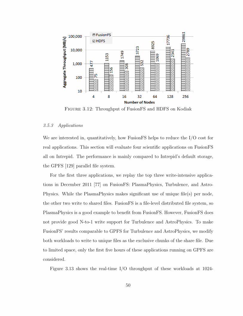
Figure 3.12: Throughput of FusionFS and HDFS on Kodiak

3.5.3 Applications

We are interested in, quantitatively, how FusionFS helps to reduce the I/O cost for

real applications. This section will evaluate four scientific applications on FusionFS

all on Intrepid. The performance is mainly compared to Intrepid’s default storage,

the GPFS [129] parallel file system.

For the first three applications, we replay the top three write-intensive applica-

tions in December 2011 [77] on FusionFS: PlasmaPhysics, Turbulence, and Astro-

Physics. While the PlasmaPhysics makes significant use of unique file(s) per node,

the other two write to shared files. FusionFS is a file-level distributed file system, so

PlasmaPhysics is a good example to benefit from FusionFS. However, FusionFS does

not provide good N-to-1 write support for Turbulence and AstroPhysics. To make

FusionFS’ results comparable to GPFS for Turbulence and AstroPhysics, we modify

both workloads to write to unique files as the exclusive chunks of the share file. Due

to limited space, only the first five hours of these applications running on GPFS are

considered.

Figure 3.13 shows the real-time I/O throughput of these workloads at 1024-

50

nodes. On FusionFS, these workloads are completed in 2.38, 4.97, and 3.08 hours,

for PlasmaPhysics, Turbulence, and AstroPhysics, respectively. Recall that all of

these workloads are completed in 5 hours in GPFS.

(a) PlasmaPhysics (b) Turbulence

(c) AstroPhysics

Figure 3.13: Top three write-intensive applications on Intrepid

It is noteworthy that for both the PlasmaPhysics and AstroPhysics applications,

the peak I/O rates for GPFS top at around 2GB/s while for FusionFS they reach

over 100GB/s. This increase in I/O performance accelerates the applications 2.1X

times (PlasmaPhysics) and 1.6X times (AstroPhysics). The reason why Turbulence

does not benefit much from FusionFS is that, there are not many consecutive I/O

operations in this application and GPFS is sufficient for such workload patterns: the

heavy interleaving of I/O and computation does not push much I/O pressure to the

51

storage system.

The fourth application, Basic Local Alignment Search Tool (BLAST), is a popular

bioinformatics application to benchmark parallel and distributed systems. BLAST

searches one or more nucleotide or protein sequences against a sequence database

and calculates the similarities. It has been implemented with different parallelized

frameworks, e.g. ParallelBLAST [87]. In ParallelBLAST, the entire database (4GB)

is split into smaller chunks on different nodes. Each node then formats its chunk

into an encoded slice, and searches protein sequence against the slice. All the search

results are merged together into the final matching result.

We compared ParallelBLAST performance on FusionFS and GPFS with our AME

(Any-scale MTC Engine) framework [169]. We carried out a weak scaling experiment

of ParallelBLAST with 4GB database on every 64-nodes, and increased the database

size proportionally to the number of nodes. The application has three stages (for-

matdb, blastp, and merge), which produces an overall data I/O of 541GB over 16192

files for every 64-nodes. Figure 3.14 shows the workload in all three stages and the

number of accessed files from 1 node to 1024 nodes. In our experiment of 1024-node

scale, the total I/O is about 9TB applied to over 250,000 files.

Figure 3.14: The workload over three stages of BLAST

As shown in Figure 3.15, there is a huge (more than one order of magnitude)

52

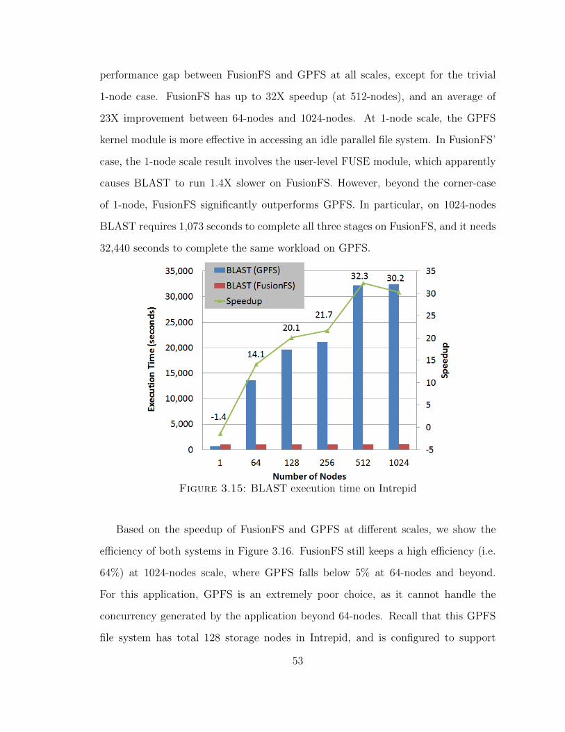
performance gap between FusionFS and GPFS at all scales, except for the trivial

1-node case. FusionFS has up to 32X speedup (at 512-nodes), and an average of

23X improvement between 64-nodes and 1024-nodes. At 1-node scale, the GPFS

kernel module is more effective in accessing an idle parallel file system. In FusionFS’

case, the 1-node scale result involves the user-level FUSE module, which apparently

causes BLAST to run 1.4X slower on FusionFS. However, beyond the corner-case

of 1-node, FusionFS significantly outperforms GPFS. In particular, on 1024-nodes

BLAST requires 1,073 seconds to complete all three stages on FusionFS, and it needs

32,440 seconds to complete the same workload on GPFS.

Figure 3.15: BLAST execution time on Intrepid

Based on the speedup of FusionFS and GPFS at different scales, we show the

efficiency of both systems in Figure 3.16. FusionFS still keeps a high efficiency (i.e.

64%) at 1024-nodes scale, where GPFS falls below 5% at 64-nodes and beyond.

For this application, GPFS is an extremely poor choice, as it cannot handle the

concurrency generated by the application beyond 64-nodes. Recall that this GPFS

file system has total 128 storage nodes in Intrepid, and is configured to support

53

concurrent accessing from 40K compute nodes, yet it exhibits little scaling from as

small as 64-nodes.

Figure 3.16: BLAST I/O efficiency on Intrepid

Lastly, we measure the overall throughput of data I/O at different scales as gener-

ated by the BLAST application in Figure 3.17. FusionFS has an excellent scalability

reaching over 8GB/s, and GPFS is saturated at 0.27GB/s from 64 nodes and beyond.

Figure 3.17: BLAST I/O throughput on Intrepid

54

Load balance. The I/O strategy of FusionFS is optimized for file write, and

does not take load balance into account. Recall that every client tries to write

memory to the local disk, even for those files whose original location is a remote

node. FusionFS just updates the metadata instead of sending back the updated file

to its original location. So for those workloads where a subset of active nodes conduct

significantly more file writes than other nodes, we expect more data to reside on these

active nodes, which puts the system in an imbalance state of storage consumption.

This issue could be addressed by an asynchronous re-balance procedure running in

the background, or by a load-aware task scheduler that steals tasks from the active

nodes to the more idle ones.

N-to-1 Write. The current FusionFS implementation works on the file granu-

larity. This implies that multiple nodes concurrently writing to different portions of

the same file would cause a non-deterministic result. While we could manually split

the file into sub-files of exclusive chunks to be accessed concurrently, a more elegant

solution would be for FusionFS to provide an API or runtime option to turn on this

chunk-level manipulation.

3.6 Summary

This chapter introduces a distributed storage layer on compute nodes to tackle the

HPC I/O bottleneck of scientific applications. We identify the challenges this un-

precedented architecture brings, and build a distributed file system FusionFS to

tackle them. In particular, FusionFS is crafted to support extremely intensive meta-

data operations and is optimized for file writes. Extreme-scale evaluation on up to

16K nodes demonstrates FusionFS’ superiority over other popular storage systems

for scientific applications.

55

4

Caching Middleware for Distributed and ParallelFilesystems

One of the bottlenecks of distributed file systems deals with mechanical hard drives

(HDD). Although solid-state drives (SSD) have been around since the 1990’s, HDDs

are still dominant due to large capacity and relatively low cost. Hybrid hard drives

with a small built-in SSD cache does not meet the need of a large variety of workloads.

This section proposes a middleware that manages the underlying heterogeneous

storage devices in order to allow distributed file systems to leverage the SSD perfor-

mance while leveraging the capacity of HDD. We design and implement a user-level

filesystem, HyCache [174], that can offer SSD-like performance at a cost similar to

a HDD. We show how HyCache can be used to improve performance in distributed

file systems, such as the Hadoop HDFS.

We then extend HyCache to HyCache+ [171] –a cooperative cache on the com-

pute nodes–, which allows I/O to effectively leverage the high bi-section bandwidth

of the high-speed interconnect of massively parallel high-end computing systems.

HyCache+ provides the POSIX interface to end users with the memory-class I/O

56

throughput and latency, and transparently swap the cached data with the existing

slow-speed but high-capacity networked attached storage. HyCache+ has the po-

tential to achieve both high performance and low-cost large capacity, the best of

both worlds. To further improve the caching performance from the perspective of

the global storage system, we propose a 2-phase mechanism to cache the hot data

for parallel applications, called 2-Layer Scheduling (2LS), which minimizes the file

size to be transferred between compute nodes and heuristically replaces files in the

cache.

4.1 HyCache: Local Caching with Memory-Class Storage

HyCache is designed to manage heterogeneous storage devices for distributed filesys-

tems. HyCache provides standard POSIX interfaces through FUSE [40] and works

completely in the user space. We show that in the context of filesystems, the overhead

of user-level APIs (i.e. libfuse) is negligible with multithread support on SSD, and

with appropriate tuning can even outperform the kernel-level implementation. The

user-space feature of HyCache allows non-privileged users to specify the SSD cache

size, an invaluable feature in making HyCache more versatile and flexible to support

a much wider array of workloads. Furthermore, distributed or parallel filesystems

can leverage HyCache without any modifications through its POSIX interface. This

is critical in many cases where the end users are not allowed to modify the kernel of

HPC systems. Figure 4.1 shows the conceptual view of the storage hierarchy with

HyCache. Instead of being mounted directly on the native file systems (e.g. Linux

Ext4), distributed file systems are deployed on top of HyCache on all data nodes.

4.1.1 Design Overview

Figure 4.2 shows a bird’s view of HyCache as a middleware between distributed file

systems and local storages. At the highest level there are three logical components:

57

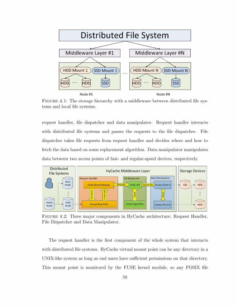
Figure 4.1: The storage hierarchy with a middleware between distributed file sys-tems and local file systems.

request handler, file dispatcher and data manipulator. Request handler interacts

with distributed file systems and passes the requests to the file dispatcher. File

dispatcher takes file requests from request handler and decides where and how to

fetch the data based on some replacement algorithm. Data manipulator manipulates

data between two access points of fast- and regular-speed devices, respectively.

Figure 4.2: Three major components in HyCache architecture: Request Handler,File Dispatcher and Data Manipulator.

The request handler is the first component of the whole system that interacts

with distributed file systems. HyCache virtual mount point can be any directory in a

UNIX-like system as long as end users have sufficient permissions on that directory.

This mount point is monitored by the FUSE kernel module, so any POSIX file

58

operations on this mount point is passed to the FUSE kernel module. Then the

FUSE kernel module will import the FUSE library and try to transfer the request

to FUSE API in the file dispatcher.

File dispatcher is the core component of HyCache, as it redirects user-provided

POSIX requests into customized handlers of file manipulations. FUSE only provides

POSIX interfaces and file dispatcher is exactly the place where these interfaces are

implemented, e.g. some of the most important file operations like open(), read() and

write(), etc. File dispatcher manages the file locations and determines with which

hard drive a particular file should be dealing. Some replacement policies, i.e. cache

algorithms, need to be provided to guide the File Dispatcher.

Cache algorithms are optimizing instructions that a computer program can follow

to manage a cache of information stored on the computer. When the cache is full,

the algorithm must choose which items to discard to make room for the new ones.

In case of HyCache, cache algorithm determines which file(s) in SSD are swapped to

HDD when the SSD space is intensive. Different cache algorithms have been exten-

sively studied in the past decades. There is no one single algorithm that suppresses

others in all scenarios. We have implemented LRU (Least Recently Used) and LFU

(Least Frequently Used) [137] in HyCache and the users are free to plug in their own

algorithms for swapping files.

Data manipulator manipulates data between two logical access points: one for

fast speed access, i.e. SSDs and the other is for regular access e.g. HDDs. An access

point is not necessarily a mount point of a device in the local operating system,

but a logical view of any combination of these mount points. In the simplest case,

Access point A could be the SSD mount point whereas access Point B is set to the

HDD mount point. Access point A is always the preferred point for any data request

as long as it has enough space based on some user defined criteria. Data need to

be swapped back and forth between A and B once the space usage in A exceeds

59

some threshold. For simplicity we only show Access point A and B in the figure,

however there is nothing architecturally that prohibits us from leveraging more than

two levels of access points.

4.1.2 User Interface

The HyCache mount point itself is not only a single local directory but a virtual

entry point of two mount points for SSD partition and HDD partition, respectively.

Figure 4.3 shows how to mount HyCache in a UNIX-like system. Assuming HyCache

would be mounted on a local directory called hycache mount, and another local

directory (e.g. hycache root) has been created and has at least two subdirectories:

the mount point of the SSD partition and the mount point of the HDD partition, users

can simply execute ./hycache ărootą ămountą where hycache is the executable for

HyCache, root is the physical directory and mount is the virtual directory.

Figure 4.3: How to mount HyCache in a UNIX-like machine.

4.1.3 Strong Consistency

We keep only one single copy of any file at any time to achieve strong consistency.

For manipulating files across multiple storage devices we use symbolic links to track

60

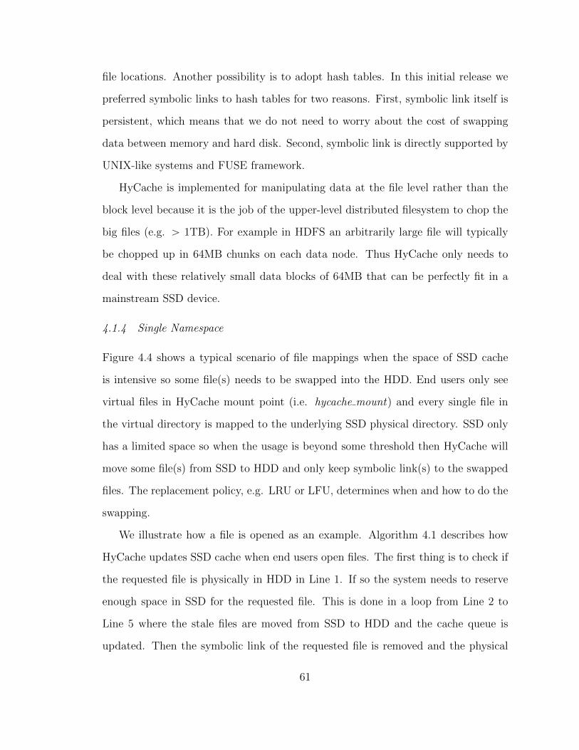
file locations. Another possibility is to adopt hash tables. In this initial release we

preferred symbolic links to hash tables for two reasons. First, symbolic link itself is

persistent, which means that we do not need to worry about the cost of swapping

data between memory and hard disk. Second, symbolic link is directly supported by

UNIX-like systems and FUSE framework.

HyCache is implemented for manipulating data at the file level rather than the

block level because it is the job of the upper-level distributed filesystem to chop the

big files (e.g. ą 1TB). For example in HDFS an arbitrarily large file will typically

be chopped up in 64MB chunks on each data node. Thus HyCache only needs to

deal with these relatively small data blocks of 64MB that can be perfectly fit in a

mainstream SSD device.

4.1.4 Single Namespace

Figure 4.4 shows a typical scenario of file mappings when the space of SSD cache

is intensive so some file(s) needs to be swapped into the HDD. End users only see

virtual files in HyCache mount point (i.e. hycache mount) and every single file in

the virtual directory is mapped to the underlying SSD physical directory. SSD only

has a limited space so when the usage is beyond some threshold then HyCache will

move some file(s) from SSD to HDD and only keep symbolic link(s) to the swapped

files. The replacement policy, e.g. LRU or LFU, determines when and how to do the

swapping.

We illustrate how a file is opened as an example. Algorithm 4.1 describes how

HyCache updates SSD cache when end users open files. The first thing is to check if

the requested file is physically in HDD in Line 1. If so the system needs to reserve

enough space in SSD for the requested file. This is done in a loop from Line 2 to

Line 5 where the stale files are moved from SSD to HDD and the cache queue is

updated. Then the symbolic link of the requested file is removed and the physical

61

Figure 4.4: File movement in HyCache. When free space of SSD cache is belowsome threshold, based on some caching algorithm file2 is evicted out of the SSD.The SSD cache still keeps a symbolic link of file2 which has been moved to the HDDdrive.

one is moved from HDD to SSD in Line 6 and Line 7. We also need to update the

cache queue in Line 8 and Line 10 for two scenarios, respectively. Finally the file is

opened in Line 12.

Another important file operation in HyCache that is worth mentioning is file

removal. We explain how HyCache removes a file in Algorithm 4.2. Line 4 and Line

5 are standard instructions used in file removal: update the cache queue and remove

62

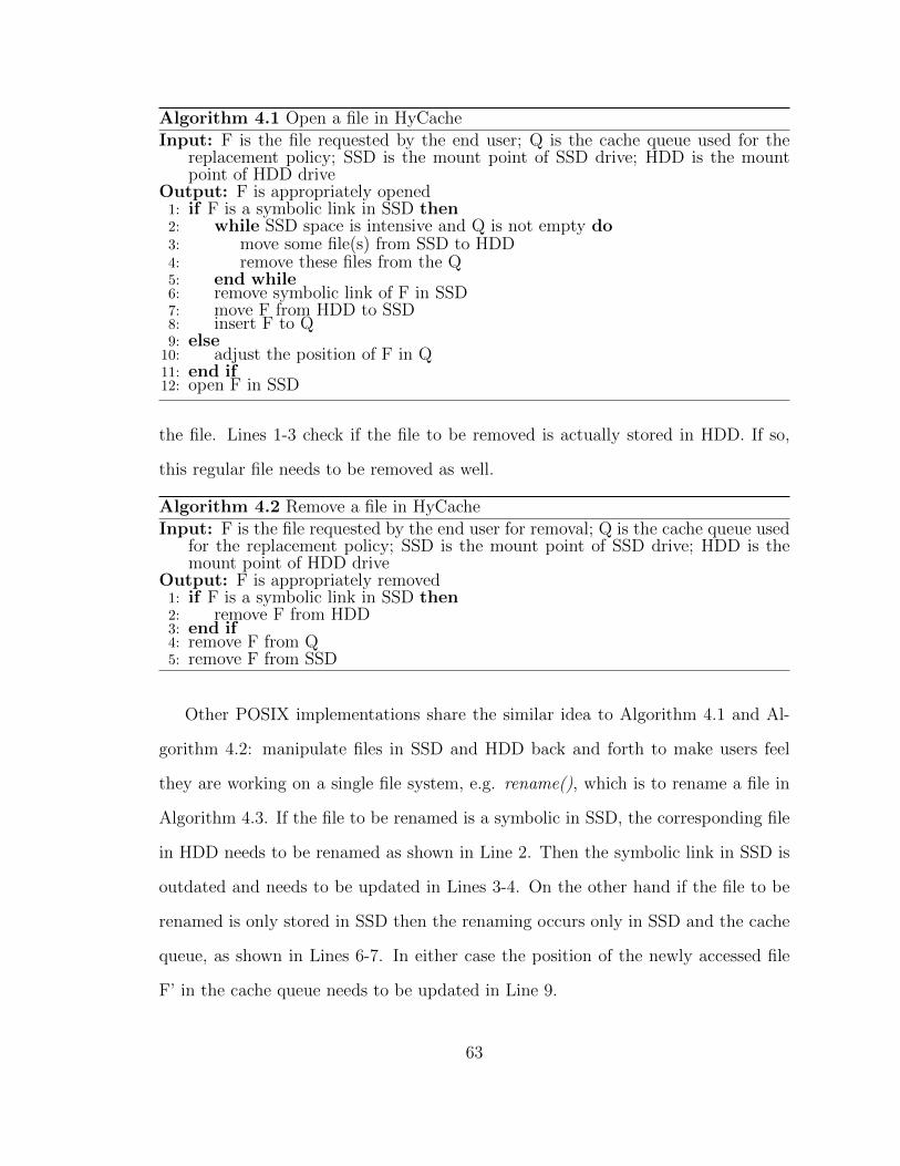
Algorithm 4.1 Open a file in HyCache

Input: F is the file requested by the end user; Q is the cache queue used for thereplacement policy; SSD is the mount point of SSD drive; HDD is the mountpoint of HDD drive

Output: F is appropriately opened1: if F is a symbolic link in SSD then2: while SSD space is intensive and Q is not empty do3: move some file(s) from SSD to HDD4: remove these files from the Q5: end while6: remove symbolic link of F in SSD7: move F from HDD to SSD8: insert F to Q9: else

10: adjust the position of F in Q11: end if12: open F in SSD

the file. Lines 1-3 check if the file to be removed is actually stored in HDD. If so,

this regular file needs to be removed as well.

Algorithm 4.2 Remove a file in HyCache

Input: F is the file requested by the end user for removal; Q is the cache queue usedfor the replacement policy; SSD is the mount point of SSD drive; HDD is themount point of HDD drive

Output: F is appropriately removed1: if F is a symbolic link in SSD then2: remove F from HDD3: end if4: remove F from Q5: remove F from SSD

Other POSIX implementations share the similar idea to Algorithm 4.1 and Al-

gorithm 4.2: manipulate files in SSD and HDD back and forth to make users feel

they are working on a single file system, e.g. rename(), which is to rename a file in

Algorithm 4.3. If the file to be renamed is a symbolic in SSD, the corresponding file

in HDD needs to be renamed as shown in Line 2. Then the symbolic link in SSD is

outdated and needs to be updated in Lines 3-4. On the other hand if the file to be

renamed is only stored in SSD then the renaming occurs only in SSD and the cache

queue, as shown in Lines 6-7. In either case the position of the newly accessed file

F’ in the cache queue needs to be updated in Line 9.

63

Algorithm 4.3 Rename a file in HyCache

Input: F is the file requested by the end user to rename; F’ is the new file name;Q is the queue used for the replacement policy; SSD is the mount point of SSDdrive; HDD is the mount point of HDD drive

Output: F is renamed to F’1: if F is a symbolic link in SSD then2: rename F to F’ in HDD3: remove F in SSD4: create the symbolic link F’ in SSD5: else6: rename F to F’ in SSD7: rename F to F’ in Q8: end if9: update F’ position in Q

4.1.5 Caching Algorithms

HyCache provides two built-in cache algorithms: LRU and LFU. End users are free

to plug in other cache algorithms depending on their data patterns and application

characteristics. As shown in Algorithms 4.1, all the implementations are independent

of specific cache algorithms. LRU is one of the most widely used cache algorithms in

computer systems. It is also the default cache algorithm used in HyCache. LFU is

an alternative to facilitate the SSD cache if the access frequency is of more interests.

In case all files are only accessed once (or for equal times), LFU is essentially the

same as LRU, i.e. the file that is least recently used would be swapped to HDD if

SSD space becomes intensive. We implement LRU and LFU with the standard C

library ăsearch.hą instead of importing any third-party libraries for queue-handling

utilities. This header supports doubly-linked list with only two operation: insque()

for insertion and remque() for removal. We implement all other utilities from scratch

e.g. check the queue length, search for a particular element in the queue, etc. Each

element of LRU and LFU queues stores some metadata of a particular file like file-

name, access time, number of access (only useful for LFU though), etc.

Figure 4.5 illustrates how LRU is implemented for HyCache. A new file is always

created on SSD. This is possible because HyCache ensures the SSD partition has

enough space for next file operation after current file operation. For example after

64

editing a file, the system checks if the usage of SSD has hit the threshold of being

considered as “SSD space is intensive”. Users can define this value by their own, for

example 90% of the entire SSD. When the new file has been created on SSD it is also

inserted in to the tail of LRU queue. On the other hand, if the SSD space is intensive

we need to keep swapping the heads of LRU queue into HDD until the SSD usage is

below the threshold. Both cases are pretty standard queue operations as shown in

the top part of Figure 4.5. If a file already in the LRU queue gets accessed then we

need to update its position in the LRU queue to reflect the new time stamp of this

file. In particular, as shown in the bottom part of Figure 4.5, the newly accessed file

needs to be removed from the queue and re-inserted into the tail.

Figure 4.5: LRU queue in HyCache.

LFU is implemented in a similar way as LRU with a little more work. In LFU,

the position of a file in the queue is determined by two criteria: frequency and

timestamp. LFU first checks the access frequency of the file. The more frequently

this file has been touched, the closer it will be positioned to the queue tail. If there

are multiple files with the same frequency, for this particular set of files LRU will be

applied, i.e. based on timestamp.

4.1.6 Multithread Support

HyCache fully supports multithreading to leverage the many-core architecture in

most high performance computers. Users have the option to disable this feature

65

to run applications in the single-thread mode. Even though there are cases where

multithreading does not help and only introduces overheads by switching contexts,

by default multithreading is enabled in HyCache because in most cases this would

improve the overall performance by keeping the CPU busy. We will see in the

evaluation section how the aggregate throughput is significantly elevated with the

help of concurrency.

4.2 HyCache+: Cooperative Caching among Many Nodes

This section presents a distributed storage middleware, called HyCache+, right on

the compute nodes, which allows I/O to effectively leverage the high bi-section band-

width of the high-speed interconnect of massively parallel high-end computing sys-

tems. HyCache+ provides the POSIX interface to end users with the memory-class

I/O throughput and latency, and transparently swap the cached data with the ex-

isting slow-speed but high-capacity networked attached storage. HyCache+ has the

potential to achieve both high performance and low-cost large capacity, the best of

both worlds. To further improve the caching performance from the perspective of

the global storage system, we propose a 2-phase mechanism to cache the hot data

for parallel applications, called 2-Layer Scheduling (2LS), which minimizes the file

size to be transferred between compute nodes and heuristically replaces files in the

cache.

Figure 4.6 shows the design overview of HyCache+, on an oversimplified 2-node

cluster. A job scheduler deploys a job on a specific machine, Node 1 in this example.

The hot files are accessed from the local cache if possible, and can potentially be

replaced by the cold files in the remote parallel file systems according to the caching

algorithm, e.g. LRU or Algorithm 4.5 that will be presented in §4.2.2. The hot

files could be migrated between compute nodes with extremely high throughput

and low latency, since most HPC systems are deployed with high-speed interconnect

66

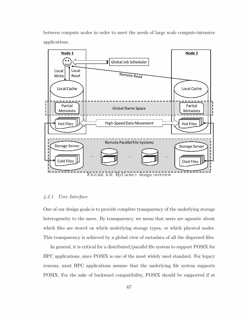
between compute nodes in order to meet the needs of large scale compute-intensive

applications.

Figure 4.6: HyCache+ design overview

4.2.1 User Interface

One of our design goals is to provide complete transparency of the underlying storage

heterogeneity to the users. By transparency, we mean that users are agnostic about

which files are stored on which underlying storage types, or which physical nodes.

This transparency is achieved by a global view of metadata of all the dispersed files.

In general, it is critical for a distributed/parallel file system to support POSIX for

HPC applications, since POSIX is one of the most widely used standard. For legacy

reasons, most HPC applications assume that the underlying file system supports

POSIX. For the sake of backward compatibility, POSIX should be supported if at

67

all possible. HyCache+ leverages the FUSE framework [40] to support POSIX.

The FUSE kernel module has been officially merged into the Linux kernel tree

since kernel version 2.6.14. FUSE provides 35 interfaces to fully comply with POSIX

file operations. Some of these are called more frequently e.g. some essential file oper-

ations like open(), read(), write() and unlink(), whereas others might be less popular

or even remain optional in some Linux distributions like getxattr() and setxattr()

which are to get and set extra file attributes, respectively.

FUSE has been criticized for its efficiency on traditional HDD-based file systems.

In native UNIX file systems (e.g. Ext4) there are only two context switches between

the caller in user space and the system call in kernel spaces. However for a FUSE-

based file system, context needs to be switched four times: two switches between

the caller and the virtual file system; and another two between libfuse and FUSE.

We will show that this overhead, at least in HPC systems when multi-threading is

turned on, is insignificant (§4.3.1).

HyCache+ is deployed as a user level mount point in accordance with other user

level file systems. The mount point itself is a virtual entry point that talks to the local

cache and remote parallel file system. For example (see Figure 4.7), HyCache+ could

be mounted on a local directory called /mnt/hycacheplus/, while two other physical

directories /dev/ssd/ and /mnt/gpfs/ ) are for the local cache and the remote parallel

file system, respectively.

4.2.2 Job Scheduling

The variables to be used in the discussion are summarized in Table 4.1. If the

application needs to access a file Fi on a remote machine, the overhead on transferring

Fi is SizepFiq.

We formalize the problem as to find the matrix Q (i.e. scheduling which job on

which machine) that minimizes the overall network cost of running all |A| jobs on

68

Figure 4.7: HyCache+ mountpoint

Table 4.1: Variables of global scheduling

Variable Type Meaning

M Set Machines of the clusterA Set Applications to be runF Set All filesF k Set Files referenced by Ak P APi,j Int Fi P F placed on Mj PMQi,j Int Ai P A scheduled on Mj PM

|M | machines. That is to solve the objective function

arg minQ

ÿ

AkPA

ÿ

MlPM

ÿ

FiPFk

ÿ

MjPM

SizepFiq ¨ Pi,j ¨Qk,l,

subject toÿ

MjPM

Pi,j “ 1, @Fi P F,

ÿ

MjPM

Qi,j “ 1, @Ai P A,

Pi,j, Qi,j P t0, 1u, @i, j.

The first constraint guarantees that a file could be placed on exact one node.

Similarly, the second constraints guarantees that a job could be scheduled on exact

one node. Note that both constraints could be generalized by replacing 1 with other

69

constants if needed, for example in distributed file systems [134] a file could have

multiple replicas for high reliability. The last constraint says that both matrices

should only store binary values to guarantee the first and the second constraints.

The algorithm to find the machine for a job to achieve the minimal network cost

is given in Algorithm 4.4. The input is the job index x, and it returns the machine

index y. It loops on each machine (Line 4), calculates the cost of moving all the

referenced files to this machine (Lines 5 - 9), and updates the minimal cost if needed

(Lines 10 - 13).

Algorithm 4.4 Global Schedule

Input: The xth job to be scheduledOutput: The yth machine where the xth job should be scheduled

1: function GlobalSchedule(x)2: MinCostÐ 83: y Ð NULL4: for Mi PM do5: CostÐ 06: for Fj P F

x do7: Find Mk such that Pj,k “ 18: CostÐ Cost` SizepFjq

9: end for10: if Cost ăMinCost then11: MinCostÐ Cost12: y Ð i13: end if14: end for15: return y16: end function

The correctness of Algorithm 4.4 is due to the fact that the data locality is

known as a priori input. That is, P is a given argument to the execution of all jobs.

Otherwise Line 7 would not work appropriately. The per-job networking overhead is

obviously minimal. Since jobs are assumed independent, the overall overhead of all

jobs is also minimal.

The complexity of Algorithm 4.4 is Op|M | ¨ |Fx|q, by observing the two loops on

Line 4 and Line 6, respectively. Note that we could achieve an Op1q cost for Line 7

by retrieving the metadata of file j.

70

4.2.3 Heuristic Caching

Problem Statement. The problem of finding optimal caching on multiple-disk is

proved to be NP-hard [6]. A simpler problem on a single-disk setup has a poly-

nomial solution [2], which is, unfortunately, too complex to be applied in real ap-

plications. An approximation algorithm was proposed in [18] with the restriction

that each file size should be the same, which limits its use in practice. In fact, at

small scale (e.g. each node has Op10q files to access), a brute-force solution with dy-

namic programming is viable, with the same idea of the classical problem of traveling

salesman problem (TSP) [10] with exponential time complexity. However, in real ap-

plications the number of accessed files could be as large as 10,000, which makes the

dynamic programming approach feasible. Therefore we propose a heuristic algorithm

of Opn lg nq (n is the number of distinct files on the local node) for each job, which

is efficient enough for arbitrarily large number of files in practice, especially when

compared to the I/O time of the disk.

Assumptions. We assume a queue of jobs, and their requested files are known on

each node in a given period of time, which could be calculated from the scheduling

results of §4.2.2 and the metadata information. This assumption is based on our

observation of many workflow systems [183, 184], which implicitly make a similar

assumption: users are familiar with the applications they are to run and they are

able to specify the task dependency (often times automatically based on the high-

level parallel workflow description). Note that the referenced files are only for the

jobs deployed on this node, because there is no need to cache the files that will be

accessed by the jobs deployed on remote nodes.

Notations and Definitions The access pattern of a job is represented by a sequence

R “ pr1, r2, . . . , rmq, where each ri indicates one access to a particular file. Note that

the files referenced by different ri’s are possibly the same, and could be on the

71

cache, or the disk. We use Filepriq to indicate the file object which ri references

to. The size of the referenced file by ri is denoted by SizepFilepriqq. The cost

is defined as the to-be-evicted file size multiplied by its access frequency after the

current processing position in the reference sequence. The gain is defined as the to-

be-cached file size multiplied by its access frequency after the current fetch position

in the reference sequence. Since cache throughput is typically orders of magnitude

higher than disks (i.e. O(10GB/s) vs. O(100MB/s)), in our analysis we ignore the

time of transferring data between the processor and the cache. Similarly, when the

file is swapped between cache and disks, only the disk throughput is counted. The

cache size on the local node is denoted by C, and the current set of files in the cache is

denoted by S. Our goal is to minimize the total I/O cost of the disk by determining

whether the accessed files should be placed in the cache.

There are 3 rules to be followed in the proposed caching algorithms.

Rule 1. Every fetch should bring into the cache the very next file in the reference

sequence if it is not yet in the cache.

Rule 2. Never fetch a file to the cache if the total cost of the to-be-evicted files

is greater than the gain of fetching this file.

The first 2 rules specify which file to be fetched and when to do the fetch, and

say nothing about evicting files. Rule 3 speaks about what files to be evicted and

when to do the eviction.

Rule 3. Every fetch should discard the files in the increasing order of their cost

until there is enough space for the newly fetched file. If the cache has enough space

for the new file, no eviction is needed.

We elucidate the above 3 rules with a concrete example. Assume we have a

random reference sequence R “ pr1, r2, r3, r4, r5, r6, r7, r8, r9q. Let Filepr1q “ F1,

Filepr2q “ F2, Filepr3q “ F3, Filepr4q “ F4, Filepr5q “ F3, Filepr6q “ F1,

Filepr7q “ F2, Filepr8q “ F4, Filepr9q “ F3, and SizepF1q “ 20, SizepF2q “ 40,

72

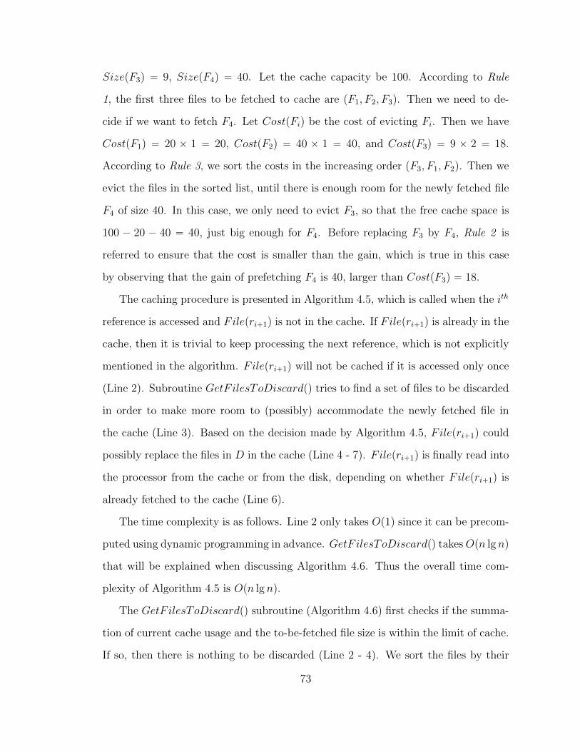
SizepF3q “ 9, SizepF4q “ 40. Let the cache capacity be 100. According to Rule

1, the first three files to be fetched to cache are pF1, F2, F3q. Then we need to de-

cide if we want to fetch F4. Let CostpFiq be the cost of evicting Fi. Then we have

CostpF1q “ 20 ˆ 1 “ 20, CostpF2q “ 40 ˆ 1 “ 40, and CostpF3q “ 9 ˆ 2 “ 18.

According to Rule 3, we sort the costs in the increasing order pF3, F1, F2q. Then we

evict the files in the sorted list, until there is enough room for the newly fetched file

F4 of size 40. In this case, we only need to evict F3, so that the free cache space is

100 ´ 20 ´ 40 “ 40, just big enough for F4. Before replacing F3 by F4, Rule 2 is

referred to ensure that the cost is smaller than the gain, which is true in this case

by observing that the gain of prefetching F4 is 40, larger than CostpF3q “ 18.

The caching procedure is presented in Algorithm 4.5, which is called when the ith

reference is accessed and Filepri`1q is not in the cache. If Filepri`1q is already in the

cache, then it is trivial to keep processing the next reference, which is not explicitly

mentioned in the algorithm. Filepri`1q will not be cached if it is accessed only once

(Line 2). Subroutine GetF ilesToDiscardpq tries to find a set of files to be discarded

in order to make more room to (possibly) accommodate the newly fetched file in

the cache (Line 3). Based on the decision made by Algorithm 4.5, Filepri`1q could

possibly replace the files in D in the cache (Line 4 - 7). Filepri`1q is finally read into

the processor from the cache or from the disk, depending on whether Filepri`1q is

already fetched to the cache (Line 6).

The time complexity is as follows. Line 2 only takes Op1q since it can be precom-

puted using dynamic programming in advance. GetF ilesToDiscardpq takesOpn lg nq

that will be explained when discussing Algorithm 4.6. Thus the overall time com-

plexity of Algorithm 4.5 is Opn lg nq.

The GetF ilesToDiscardpq subroutine (Algorithm 4.6) first checks if the summa-

tion of current cache usage and the to-be-fetched file size is within the limit of cache.

If so, then there is nothing to be discarded (Line 2 - 4). We sort the files by their

73

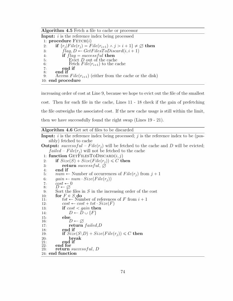
Algorithm 4.5 Fetch a file to cache or processor

Input: i is the reference index being processed1: procedure Fetch(i)2: if trj|Fileprjq “ Filepri`1q ^ j ą i` 1u ‰ H then3: flag,D Ð GetF ilesToDiscardpi, i` 1q4: if flag “ successful then5: Evict D out of the cache6: Fetch Filepri`1q to the cache7: end if8: end if9: Access Filepri`1q (either from the cache or the disk)

10: end procedure

increasing order of cost at Line 9, because we hope to evict out the file of the smallest

cost. Then for each file in the cache, Lines 11 - 18 check if the gain of prefetching

the file outweighs the associated cost. If the new cache usage is still within the limit,

then we have successfully found the right swap (Lines 19 - 21).

Algorithm 4.6 Get set of files to be discarded

Input: i is the reference index being processed; j is the reference index to be (pos-sibly) fetched to cache

Output: successful – Fileprjq will be fetched to the cache and D will be evicted;failed – Fileprjq will not be fetched to the cache

1: function GetFilesToDiscard(i, j)2: if SizepSq ` SizepFileprjqq ď C then3: return successful, H4: end if5: numÐ Number of occurrences of Fileprjq from j ` 16: gainÐ num ¨ SizepFileprjqq7: costÐ 08: D ÐH9: Sort the files in S in the increasing order of the cost

10: for F P S do11: totÐ Number of references of F from i` 112: costÐ cost` tot ¨ SizepF q13: if cost ă gain then14: D Ð D Y tF u15: else16: D ÐH17: return failed,D18: end if19: if SizepSzDq ` SizepFileprjqq ď C then20: break21: end if22: end for23: return successful, D24: end function

74

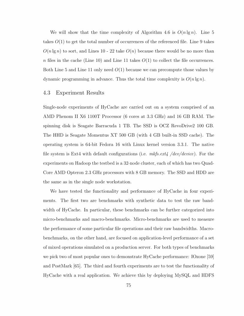
We will show that the time complexity of Algorithm 4.6 is Opn lg nq. Line 5

takes Op1q to get the total number of occurrences of the referenced file. Line 9 takes

Opn lg nq to sort, and Lines 10 - 22 take Opnq because there would be no more than

n files in the cache (Line 10) and Line 11 takes Op1q to collect the file occurrences.

Both Line 5 and Line 11 only need Op1q because we can precompute those values by

dynamic programming in advance. Thus the total time complexity is Opn lg nq.


Single-node experiments of HyCache are carried out on a system comprised of an

AMD Phenom II X6 1100T Processor (6 cores at 3.3 GHz) and 16 GB RAM. The

spinning disk is Seagate Barracuda 1 TB. The SSD is OCZ RevoDrive2 100 GB.

The HHD is Seagate Momentus XT 500 GB (with 4 GB built-in SSD cache). The

operating system is 64-bit Fedora 16 with Linux kernel version 3.3.1. The native

file system is Ext4 with default configurations (i.e. mkfs.ext4 /dev/device). For the

experiments on Hadoop the testbed is a 32-node cluster, each of which has two Quad-

Core AMD Opteron 2.3 GHz processors with 8 GB memory. The SSD and HDD are

the same as in the single node workstation.

We have tested the functionality and performance of HyCache in four experi-

ments. The first two are benchmarks with synthetic data to test the raw band-

width of HyCache. In particular, these benchmarks can be further categorized into

micro-benchmarks and macro-benchmarks. Micro-benchmarks are used to measure

the performance of some particular file operations and their raw bandwidths. Macro-

benchmarks, on the other hand, are focused on application-level performance of a set

of mixed operations simulated on a production server. For both types of benchmarks

we pick two of most popular ones to demonstrate HyCache performance: IOzone [59]

and PostMark [65]. The third and fourth experiments are to test the functionality of

HyCache with a real application. We achieve this by deploying MySQL and HDFS

75

on top of HyCache, and execute TPC-H queries [144] on MySQL and the built-in

‘sort’ application of Hadoop, respectively.

Most experiments of HyCache+ are carried out on Intrepid [58], an IBM Blue

Gene/P supercomputer of 160K cores at Argonne National Laboratory. We use up

to 1024 nodes (4096 cores) in the evaluation. Each node has a 4-core PowerPC

450 processor (850 MHz) and 2 GB of RAM. A 7.6 PB GPFS [129] is deployed

on 128 storage nodes. All experiments are repeated at least five times, or until

results become stable (i.e. within 5% margin of error); the reported numbers are the

average of all runs. Caching effect is carefully precluded by reading a file larger than

the on-board memory before the measurement.

4.3.1 FUSE Overhead

To understand the overhead introduced by FUSE in HyCache, we compare the I/O

performance between raw RAMDISK and a simple FUSE file system mounted on

RAMDISK. By experimenting on RAMDISK we completely eliminate all factors

affecting performance particularly from the spinning disk, disk controllers, etc. Since

all the I/O tests are essentially done on the memory, any noticeable performance

differences between the two setups are solely from FUSE itself.

We mount FUSE on /dev/shm, which is a built-in RAMDISK in UNIX-like sys-

tems. The read and write bandwidth on both raw RAMDISK and FUSE-based

virtual file system are reported in Figure 4.8. Moreover, the performance of con-

current FUSE processes are also plotted which shows that FUSE has a good per-

formance scalability with respect to the number of concurrent jobs. In the case of

single-process I/O, there is a significant performance gap between Ext4 and FUSE

on RAMDISK. The read and write bandwidth of Ext4 on RAMDISK are in the order

of gigabytes, whereas when mounting FUSE we could only get a bandwidth in the

range of 500 MB/s. These results suggest that FUSE could not compete with the

76

kernel-level file systems in raw bandwidth, primarily due to the overheads incurred

by having the file system in user-space, the extra memory copies, and the additional

context switching. However, we will see in the following subsections that even with

FUSE overhead on SSD, HyCache still outperforms traditional spinning disks signif-

icantly, and that concurrency can be used to scale up FUSE performance close to

the theoretical hardware performance (see Figure 4.11 and Figure 4.12).

4.3.2 HyCache Performance

IOzone is a general file system benchmark utility. It creates a temporary file with

arbitrary size provided by the end user and then conducts a bunch of file operations

like re-write, read, re-read, etc. In this paper we use IOzone to test the read and

write bandwidths as well as IOPS (input/output per second) on the different file

systems.

We show the throughput with a variety of block sizes ranging from 4 KB to 16

MB. For each block size we show five bandwidths from the left to the right: 1) the

theoretical bandwidth upper bound (obtained from RAMDISK), 2) HyCache, 3) a

simple FUSE file system accessing a HDD, 4) HDD Ext4 and 5) HHD Ext4.

Figure 4.9(a) shows HyCache read speed is about doubled comparing to the native

Ext4 file system for most block sizes. In particular when block size is 16 MB the peak

read speed for HyCache is over 300 MB/s. It is 2.2X speedup with respect to the

underlying Ext4 for HDD as shown in Figure 4.10(a). As for the overhead of FUSE

framework compared to the native Ext4 file system on spinning disks we see FUSE

only adds little overhead to read files at all block sizes as shown in Figure 4.10(a):

for most block sizes FUSE achieves nearly 100% performance of the native Ext4.

Similar results are also reported in a review of FUSE performance in [123]. This fact

indicates that even when the SSD cache is intensive and some files need to be swapped

between SSD and HDD, HyCache can still outperform Ext4 since the slower media

77

(a) Read Bandwidth

(b) Write Bandwidth

Figure 4.8: Bandwidth of raw RAMDISK and a FUSE file system mounted onRAMDISK. Px means x number of concurrent processes, e.g. FUSE RAMDISK P2stands for 2 concurrent FUSE processes on RAMDISK.

of HyCache (HDD FUSE in Figure 4.9), are comparable to Ext4. We will present the

application-level experimental results in the macro-benchmark subsection where we

discuss the performance when files are frequently swapped between SSD and HDD.

We can also see that the commercial HHD product performs at about the same level

78

of the HDD, likely primarily due to a small and inexpensive SSD.

(a) Read Bandwidth

(b) Write Bandwidth

Figure 4.9: IOzone bandwidth of 5 file systems.

We see a similar result of file writes in Figure 4.9(b) as file reads. Again HyCache

is about twice as fast when compared to Ext4 on spinning disks for most block sizes.

The peak write bandwidth which is almost 250 MB/s is also obtained when block

size is 16 MB, and it achieves 2.18x speedup for this block size compared to Ext4

79

(a) Read Speedup

(b) Write Speedup

Figure 4.10: HyCache and FUSE speedup over HDD Ext4.

as shown in Figure 4.10(b). Also in this figure, just like the case of file reads we see

little overhead of FUSE framework for the write operation on HDD except for 4KB

block.

Figure 4.10 shows that for small block size (i.e. 4 KB) HyCache only achieves

about 50% throughput of the native file system. This is due to the extra context

80

switches of FUSE between user level and kernel level, in which the context switches

of FUSE dominate the performance. Fortunately in most cases this small block size

(i.e. 4 KB) is more generally used for randomly read/write of small pieces of data

(i.e. IOPS) rather than high-throughput applications. Table 4.2 shows HyCache has

a far higher IOPS than other Ext4. In particular, HyCache has about 76X IOPS

as traditional HDD. The SSD portion of the HHD device (i.e. Seagate Momentus

XT) is a read-only cache, which means the SSD cache does not take effect in this

experiment because IOPS only involves random writes. This is why the IOPS of the

HHD lands in the same level of HDD rather than SSD.

Table 4.2: IOPS of different file systems

HyCache HDD Ext4 HHD Ext4

14,878 195 61

HyCache also takes advantages of the multicore’s concurrent tasking which re-

sults in a much higher aggregate throughput. The point is that HyCache avoids

reading/writing directly on the HDD so it handles multiple I/O requests concur-

rently. In contrast, traditional HDD only has a limited number of heads for read and

write operations. Figure 4.11 shows that HyCache has almost linear scalability with

the number of processes before hitting the physical limit (i.e. 306 MB/s for 4 KB

block and 578 MB/s for 64 KB block) whereas the traditional Ext4 has degraded

performance when handling concurrent I/O requests. The largest gap is when there

are 12 concurrent processes for 64KB block (578 MB/s for HyCache and 86 MB/s

for HDD): HyCache has 7X higher throughput than Ext4 on HDD.

The upper bound of aggregate throughput is limited by the SSD device rather

than HyCache. This can be demonstrated in Figure 4.12 that shows how HyCache

performs in RAMDISK. The performance of raw RAMDISK were also plotted. We

can see that the bandwidth of 64KB block can be achieved at about 4 GB/s by

81

(a) 4KB Block

(b) 64KB Block

Figure 4.11: Aggregate bandwidth of concurrent processes.

concurrent processes. This indicates that FUSE itself is not a bottle neck in the last

experiment: it will not limit the I/O speed unless the device is slow. This implies

that HyCache can be applied to any faster storage devices in future as long as the

workloads have enough concurrency to allow FUSE to harness multiple computing

cores. Another observation is that HyCache can consume as much as 35% of raw

82

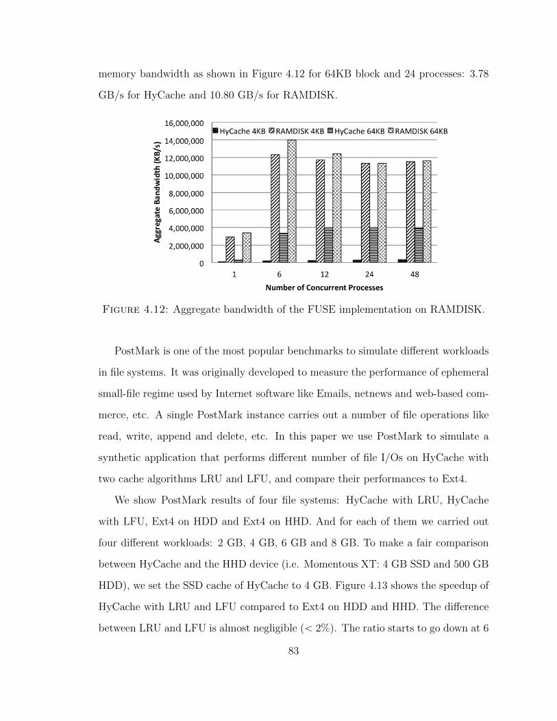
memory bandwidth as shown in Figure 4.12 for 64KB block and 24 processes: 3.78

GB/s for HyCache and 10.80 GB/s for RAMDISK.

Figure 4.12: Aggregate bandwidth of the FUSE implementation on RAMDISK.

PostMark is one of the most popular benchmarks to simulate different workloads

in file systems. It was originally developed to measure the performance of ephemeral

small-file regime used by Internet software like Emails, netnews and web-based com-

merce, etc. A single PostMark instance carries out a number of file operations like

read, write, append and delete, etc. In this paper we use PostMark to simulate a

synthetic application that performs different number of file I/Os on HyCache with

two cache algorithms LRU and LFU, and compare their performances to Ext4.

We show PostMark results of four file systems: HyCache with LRU, HyCache

with LFU, Ext4 on HDD and Ext4 on HHD. And for each of them we carried out

four different workloads: 2 GB, 4 GB, 6 GB and 8 GB. To make a fair comparison

between HyCache and the HHD device (i.e. Momentous XT: 4 GB SSD and 500 GB

HDD), we set the SSD cache of HyCache to 4 GB. Figure 4.13 shows the speedup of

HyCache with LRU and LFU compared to Ext4 on HDD and HHD. The difference

between LRU and LFU is almost negligible (ă 2%). The ratio starts to go down at 6

83

GB because HyCache only has 4 GB allocated SSD. Another reason is that PostMark

only creates temporary files randomly without any repeated pattern. In other words

it is a data stream making the SSD cache thrashes (this could be considered to be

the worst case scenario).

(a) HyCache vs. HDD (b) HyCache vs. HHD

Figure 4.13: PostMark: speedup of HyCache over Ext4 with 4 GB SSD cache.

A big advantage of HyCache is that users can freely allocate the size of the SSD

cache. In the last experiment HyCache did not work well as HHD mainly because

the data is too large to fit in the 4 GB cache. Here we show how increasing the cache

size impacts the performance. Figure 4.14 shows that if a larger SSD cache (i.e. 1GB

- 8GB) is offered then the performance is indeed better than others with as much as

a 18% performance improvement: LRU HyCache with 8GB SSD cache vs. HHD.

We have run two real world applications on HyCache: MySQL and the Hadoop.

We install MySQL 5.5.21 with database engine MySIAM, and deploy TPC-H

2.14.3 databases. TPC-H is an industry standard benchmark for databases. By

default it provides a variety size of databases (e.g. scale 1 for 1 GB, scale 10 for

10 GB, scale 100 for 100GB) each of which has eight tables. Furthermore, TPC-H

84

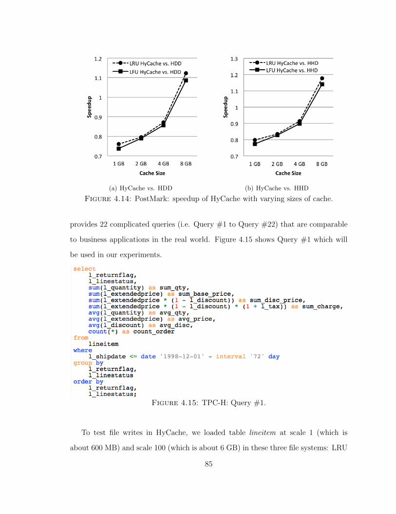
(a) HyCache vs. HDD (b) HyCache vs. HHD

Figure 4.14: PostMark: speedup of HyCache with varying sizes of cache.

provides 22 complicated queries (i.e. Query #1 to Query #22) that are comparable

to business applications in the real world. Figure 4.15 shows Query #1 which will

be used in our experiments.

Figure 4.15: TPC-H: Query #1.

To test file writes in HyCache, we loaded table lineitem at scale 1 (which is

about 600 MB) and scale 100 (which is about 6 GB) in these three file systems: LRU

85

HyCache, HDD Ext4 and HHD Ext4. As for file reads we ran Query #1 at scale

1 and scale 100. HyCache has an overall of 9% and 4% improvement over Ext4 on

HDD and HHD, respectively. The result details of these experiments are reported in

Figure 4.16.

Figure 4.16: TPC-H: speedup of HyCache over Ext4 on MySQL.

For HDFS we measure the bandwidth by concurrently copying a 1GB file per node

from HDFS to the RAMDISK (i.e. {dev{shm). The results are reported in Table 4.3,

showing that HyCache helps improve HDFS performance by 28% at 32-node scales.

We also run the built-in ‘sort’ example as a real Hadoop application. The ‘sort’

application is to use map-reduce [27] to sort a 10GB file. We kept all the default

settings in the Hadoop package except for the temporary directory which is specified

as the HyCache mount point or a local Ext4 directory. The results are reported in

Table 4.3.

Table 4.3: HDFS Performance

w/o HyCache w/ HyCache Improvement

bandwidth 114 MB/sec 146 MB/sec 28%sort 2087 sec 1729 sec 16%

86

4.3.3 HyCache+ Performance

We illustrate how HyCache+ significantly improves the I/O throughput of parallel

file systems. The local cache size is set to 256 MB (0.25 GB) on each node. To

measure local cache’s stable throughput, each client repeatedly writes a 256 MB file

for 63 times (total 15.75 GB). Then another 256 MB file is written on each client to

trigger the swapping between local cache and GPFS. Figure 4.17 reports (at 256-core

scale) the real-time aggregate throughput, showing a significant performance drop

at around 90-second timestamp, when the 15.75GB data are finished on the local

cache.

Figure 4.17: Throughput on Blue Gene/P (256 cores)

We demonstrate the scalability of HyCache+ by repeating the experiment of the

same per-client workload in §3.5.2 on 512 nodes (2048 cores). The real-time through-

put is reported in Figure 4.18. We see that HyCache+ shows an excellent scalability

for both the cached data and the remote data: both the caching throughput and

the disk throughput are about 8X faster than those numbers at 256-core scale in

Figure 4.17.

87

Figure 4.18: Throughput on Blue Gene/P (2048-cores)

We plug the heuristic caching and LRU algorithms into HyCache+, and simulate

their performance at 512-node scale on Intrepid. We create different sizes of data,

randomly between 6MB and 250MB, and repeatedly read these data in a round-robin

manner. The local cache size is set to 256MB. The execution time of both algorithms

is reported in Figure 4.19. Heuristic caching clearly outperforms LRU at all scales,

mainly because LRU does not consider the factors such as file size and cost-gain ratio,

which are carefully taken into account in heuristic caching. In particular, heuristic

caching outperforms LRU by 29X speedup at I/O size = 64,000GB (3,009 seconds

vs. 86,232 seconds).

4.4 Summary

This chapter presents HyCache that addresses the long-existing issue with the bot-

tleneck of local spinning hard drives in distributed file systems and proposed a

cost-effective solution to alleviate this bottleneck, aimed at delivering comparable

performance of an all SSD solution at a fraction of the cost. We proposed to add

a middleware layer between the distributed filesystem and the underlying local file

88

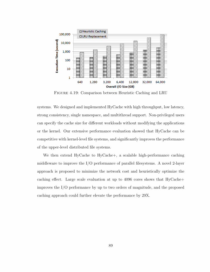
Figure 4.19: Comparison between Heuristic Caching and LRU

systems. We designed and implemented HyCache with high throughput, low latency,

strong consistency, single namespace, and multithread support. Non-privileged users

can specify the cache size for different workloads without modifying the applications

or the kernel. Our extensive performance evaluation showed that HyCache can be

competitive with kernel-level file systems, and significantly improves the performance

of the upper-level distributed file systems.

We then extend HyCache to HyCache+, a scalable high-performance caching

middleware to improve the I/O performance of parallel filesystems. A novel 2-layer

approach is proposed to minimize the network cost and heuristically optimize the

caching effect. Large scale evaluation at up to 4096 cores shows that HyCache+

improves the I/O performance by up to two orders of magnitude, and the proposed

caching approach could further elevate the performance by 29X.

89

5

Efficient Data Access in Compressible Filesystems

Data compression could ameliorate the I/O pressure of scientific applications on high-

performance computing systems. Unfortunately, the conventional wisdom of naively

applying data compression to the file or block brings the dilemma between efficient

random accesses and high compression ratios. File-level compression can barely

support efficient random accesses to the compressed data: any retrieval request need

trigger the decompression from the beginning of the compressed file. Block-level

compression provides flexible random accesses to the compressed data, but introduces

extra overhead when applying the compressor to each every block that results in a

degraded overall compression ratio.

This chapter introduces a concept called virtual chunks [179, 180] aiming to sup-

port efficient random accesses to the compressed scientific data without sacrificing

its compression ratio. In essence, virtual chunks are logical blocks identified by ap-

pended references without breaking the physical continuity of the file content. These

additional references allow the decompression to start from an arbitrary position

(efficient random access), and retain the file’s physical entirety to achieve high com-

90

pression ratio on par with file-level compression.

5.1 Background

As today’s scientific applications are becoming data-intensive, one effective approach

to relieve the I/O bottleneck of the underlying storage system is data compres-

sion. As a case in point, it is optional to apply lossless compressors (e.g. LZO [80],

bzip2 [14]) to the input or output files in the Hadoop file system (HDFS) [134], or

even lossy compressors [70, 69] at the high-level I/O middleware such as HDF5 [54]

and NetCDF [101]. By investing some computational time on compression, we hope

to significantly reduce the file size and consequently the I/O time to offset the com-

putational cost.

State-of-the-art compression mechanisms of parallel and distributed file systems,

however, simply apply the compressor to the data either at the file-level or block-

level1, and leave the important factors (e.g. computational overhead, compression

ratio, I/O pattern) to the underlying compression algorithms. In particular, we ob-

serve the following limitations of applying the file-level and block-level compression,

respectively:

1. The file-level compression is criticized by the significant overhead for random

accesses: the decompression needs to start from the very beginning of the com-

pressed file anyway even though the client might be only requesting some bytes

at an arbitrary position of the file. As a case in point, one of the most com-

monly used operations in climate research is to retrieve the latest temperature

of a particular location. The compressed data set is typically in terms of hun-

dreds of gigabytes; nevertheless scientists would need to decompress the entire

compressed file to only access the last temperature reading. This wastes both

1 The “chunk”, e.g. in HDFS, is really a file from the work node’s perspective. So “chunk-level”is not listed here.

91

the scientist’s valuable time and scarce computing resources.

2. The deficiency of block-level compression stems from its additional compression

overhead larger than the file-level counterpart, resulting in a degenerated com-

pression ratio. To see this, think about a simple scenario that a 64MB file to be

compressed with 4:1 ratio and 4 KB overhead (e.g. header, metadata, etc.). So

the resultant compressed file (i.e. file-level compression) is about 16MB+4KB

= 16.004MB. If the file is split into 64KB-blocks each of which is applied with

the same compressor, the compressed file would be 16MB+4KB*1K = 20MB.

Therefore we would roughly spend (20MB-16.004MB)/16.004MB « 25% more

space in block-level compression than the file-level one.

Virtual chunks (VC) aim to better employ existing compression algorithms in

parallel and distributed file systems, and eventually to improve the I/O performance

of random data accesses in scientific applications and high-performance computing

(HPC) systems. Virtual chunks do not break the original file into physical chunks

or blocks, but append a small number of references to the end of file. Each of

these references points to a specific block that is considered as a boundary of the

virtual chunk. Because the physical entirety (or, continuity of blocks) of the original

file is retained, the compression overhead and compression ratio keep comparable

to those of file-level compression. With these additional references, a random file

access need not decompress the entire file from the beginning, but could arbitrarily

jump onto a reference close to the requested data and start the decompression from

there. Therefore virtual chunks help to achieve the best of both file- and block-level

compressions: high compression ratio and efficient random access.

92

5.2 Virtual Chunks

To make matters more concrete, we illustrate how virtual chunks work with an

XOR-based delta compression [11] that is applied to parallel scientific applications.

The idea of XOR-based delta compression is straightforward: calculating the XOR

difference between every pair of adjacent data entries in the input file, so that only

the very first data entry needs to be stored together with the XOR differences.

This XOR compression proves to be highly effective for scientific data like climate

temperatures, because the large volume of numerical values change marginally in the

neighboring spatial and temporal area. Therefore, storing the large number of small

XOR differences instead of the original data entries could significantly shrink the size

of the compressed file.

Figure 5.1 shows an original file of eight data entries, and two references to Data 0

and Data 4, respectively. That is, we have two virtual chunks of Data 0 – 3 and Data

4 – 7, respectively. In the compressed file, we store seven deltas and two references.

When users need to read Data 7, we first copy the nearest upper reference (Ref 1 in

this case) to the beginning of the restored file, then incrementally XOR the restored

data and the deltas, until we reach the end position of the requested data. In this

example, we roughly save half of the I/O time during the random file read by avoiding

reading and decompressing the first half of the file.

For clear presentation of the following algorithms to be discussed, we assume the

original file data can be represented as a list D “ xd1, d2, . . . , dny. Since there are n

data entries, we have n´ 1 encoded data, denoted by the list X “ xx1, x2, . . . , xn´1y

where xi “ di XOR di`1 for 1 ď i ď n ´ 1. We assume there are k references (i.e.

original data entries) that the k virtual chunks start with. The k references are

represented by a list D1 “ xdc1 , dc2 , . . . , dcky, where for any 1 ď i ď k ´ 1 we have

ci ď ci`1. Notice that we need c1 “ 1, because it is the basis from where the XOR

93

Figure 5.1: Compression and decompression with two virtual chunks

could be applied to the original data D. We define L “ nk, the length of a virtual

chunk if the references are equidistant. The number in the square bracket [ ] after

a list variable indicates the index of the scalar element. For example D1ris denotes

the ith reference in the reference list D1. This should not be confused with dci , which

represents the cthi element in the original data list D. The sublist starting at s and

ending at t of a list D is represented as Ds,t.

5.2.1 Storing Virtual Chunks

We have considered two strategies on where to store the references: (1) put all

references together (either in the beginning or in the end); (2) keep the reference

in-place to indicate the boundary, i.e. spread out the references in the compressed

94

file. Current design takes the first strategy that stores the references together at the

end of the compressed file, as explained in the following.

The in-place references offer two limited benefits. Firstly, it saves space of pk´1q

encoded data entries (recall that k is the total number of references). For example,

Delta 4 would not be needed in Figure 5.1. Secondly, it avoids the computation on

locating the lowest upper reference at the end of the compressed file. For the first

benefit, the space saving is insignificant because encoded data are typically much

smaller than the original ones, not to mention this gain is factored by a relatively

small number of reference (k´ 1) comparing to the total number of data entries (n).

The second benefit on saving the computation time is also limited because the CPU

time on locating the reference is marginal compared to compressing the data entries.

The drawback of the in-place method is, even though not so obvious, critical: it

introduces significant overhead when decompressing a large portion of data spanning

over multiple logical chunks. To see this, let us imagine in Figure 5.1 that Ref 0 is

above Delta 1 and Ref 1 is in the place of Delta 4. If the user requests the entire

file, then the file system needs to read two raw data entries: Ref 0 (i.e. Data 0) and

Ref 1 (i.e. Data 4). Note that Data 0 and Data 4 are original data entries, and are

typically much larger than the deltas. Thus, reading these in-place references would

take significantly more time than reading the deltas, especially when the requested

data include a large number of virtual chunks. This issue does not exist in our current

design where all references are stored together at the end of file: the user only needs

to retrieve one reference (i.e. Ref 0 in this case).

5.2.2 Compression with Virtual Chunks

We use encode() (or decode()) applicable to two neighboring data entries to repre-

sent some compression (or decompression) algorithms to the file data. Certainly, it

is not always true that the compression algorithm deals with two neighboring data

95

entries; we only take this assumption for clear representation, and it would not affect

the validity of the algorithms or the analysis that follows.

The procedure to compress a file with multiple references is described in Algo-

rithm 0. The first phase of the virtual-chunk compression is to encode the original

data entries of the original file, as shown in Lines 1–3. The second phase appends k

references to the end of the compressed file, as shown in Lines 4–6.

Algorithm 5.1 VC Compress

Input: The original data D “ xd1, ¨ ¨ ¨ , dnyOutput: The encoded data X, and the reference list D1

1: for (int i = 1; i ă n; i++) do2: Xris Ð encode(di, di`1)3: end for4: for (int j = 1; j ă k; j++) do5: D1rjs Ð Dr1` pj ´ 1q ˚ Ls6: end for

The time complexity of Algorithm 0 is Opnq. Lines 1–3 obviously take Opnq to

compress the file. Lines 4–6 are also bounded by Opnq since there cannot be more

than n references in the procedure.

5.2.3 Optimal Number of References

This section answers this question: how many references should we append to the

compressed file, in order to maximize end-to-end I/O performance?

In general, more references consume more storage space, implying longer time to

write the compressed data to storage. As an extreme example, making a reference

to each data entry of the original file is not a good idea: the resulted compressed file

is actually larger than the original file. On the other hand, however, more references

yield a better chance of a closer lowest upper reference from the requested data,

which in turn speeds up the decompression for random accesses. Thus, we want

to find the number of references that has a good balance between compression and

decompression, and ultimately achieves the minimal overall time.

96

Despite many possible access patterns and scenarios, in this paper we are partic-

ularly interested in finding the number of references that results in the minimal I/O

time in the worst case: for data write, the entire file is compressed and written to the

disk; for data read, the last data entry is requested. That is, the decompression starts

from the beginning of the file and processes until the last data entry. The following

analysis is focused on this scenario, and assumes the references are equidistant.

Table 5.1: Virtual chunk parameters

Variable Description

Br Read BandwidthBw Write BandwidthWi Weight of InputWo Weight of OutputS Original File SizeR Compression RatioD Computational Time of Decompression

A few more parameters for the analysis are listed in Table 5.1. We denote the

read and the write bandwidth for the underlying file system by Br and Bw, respec-

tively. Different weights are assigned to input Wi and output Wo to reflect the access

patterns. For example if a file is written once and then read for 10 times in an

application, then it makes sense to assign more weights to the file read (Wi) than

the file write (Wo). S indicates the size of the original file to be compressed. R is

the compression ratio, so the compressed file size is SR

. D denotes the computational

time spent on decompressing the requested data, which should be distinguished from

the overall decompression time (D plus the I/O time).

The overhead introduced by additional references during compression is as follows.

The baseline is when the file is applied with the conventional compression with a

single reference. When comparing both cases, we need to apply the same compression

algorithm to be applied on the same set of data. Therefore, the computational

time should be unchanged regardless of the number of references appended to the

97

compressed file. So the overall time difference really comes from the I/O time of

writing different number of references.

Let Tc indicate the time difference between multiple references and a single ref-

erence, we have

Tc “pk ´ 1q ¨ S ¨Wo

n ¨Bw

Similarly, to calculate the potential gain during decompression with multiple

references, Td indicating the time difference in decompression between multiple ref-

erences and a single reference, is calculated as follows:

Td “pk ´ 1q ¨ S ¨Wi

k ¨R ¨Br

`pk ´ 1q ¨D ¨Wi

k

The first term of the above equation represents the time difference on the I/O part,

and the second term represents the computational part.

To minimize the overall end-to-end I/O time, we want to maximize the following

function (i.e. gain minus cost):

F pkq “ Td ´ Tc

Note that the I/O time is from the client’s (or, user’s) perspective. Technically, it

includes both the computational and I/O time of the (de)compression. By taking

the derivative on k (suppose k is continuous) and solving the following equation

d

dkpF pkqq “

S ¨Wi

R ¨Br ¨ k2`D ¨Wi

k2´S ¨Wo

Bw ¨ n“ 0,

we have

k “

c

n ¨Bw

Br

¨Wi

Wo

¨ p1

R`D ¨Br

Sq

98

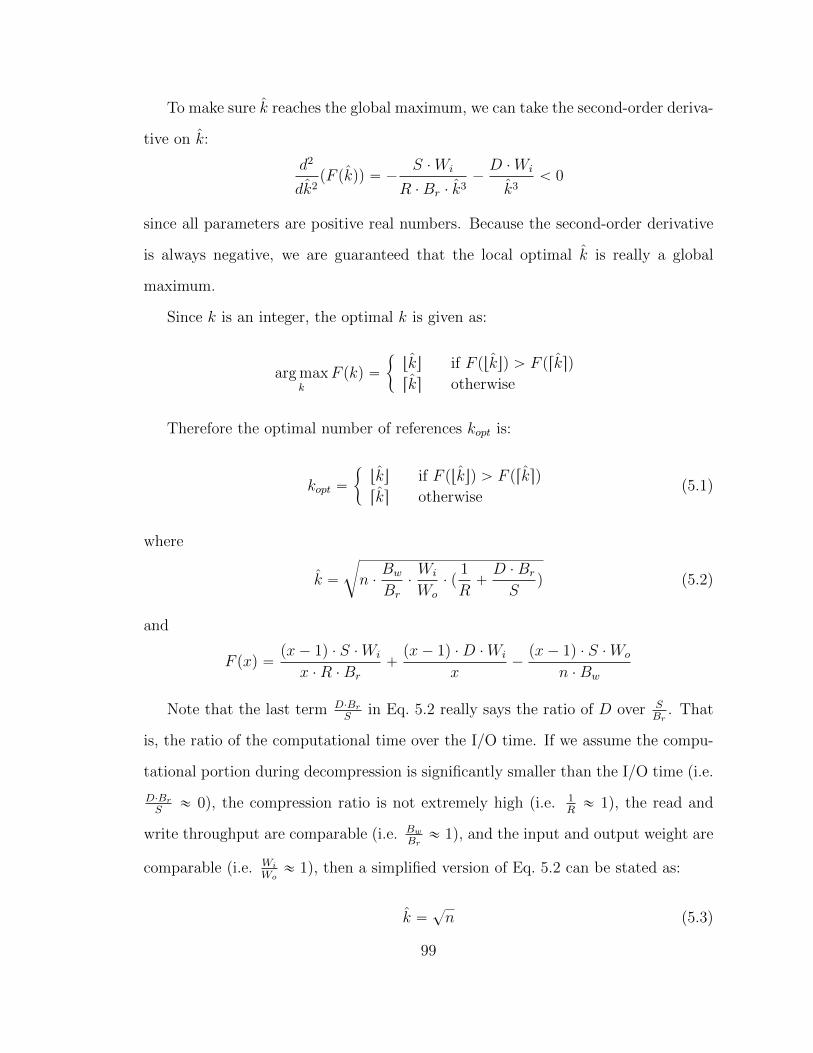
To make sure k reaches the global maximum, we can take the second-order deriva-

tive on k:

d2

dk2pF pkqq “ ´

S ¨Wi

R ¨Br ¨ k3´D ¨Wi

k3ă 0

since all parameters are positive real numbers. Because the second-order derivative

is always negative, we are guaranteed that the local optimal k is really a global

maximum.

Since k is an integer, the optimal k is given as:

arg maxk

F pkq “

"

tku if F ptkuq ą F prksq

rks otherwise

Therefore the optimal number of references kopt is:

kopt “

"

tku if F ptkuq ą F prksq

rks otherwise(5.1)

where

k “

c

n ¨Bw

Br

¨Wi

Wo

¨ p1

R`D ¨Br

Sq (5.2)

and

F pxq “px´ 1q ¨ S ¨Wi

x ¨R ¨Br

`px´ 1q ¨D ¨Wi

x´px´ 1q ¨ S ¨Wo

n ¨Bw

Note that the last term D¨Br

Sin Eq. 5.2 really says the ratio of D over S

Br. That

is, the ratio of the computational time over the I/O time. If we assume the compu-

tational portion during decompression is significantly smaller than the I/O time (i.e.

D¨Br

S« 0), the compression ratio is not extremely high (i.e. 1

R« 1), the read and

write throughput are comparable (i.e. Bw

Br« 1), and the input and output weight are

comparable (i.e. Wi

Wo« 1), then a simplified version of Eq. 5.2 can be stated as:

k “?n (5.3)

99

suggesting that the optimal number of references be roughly the squared root of the

total number of data entries.

5.2.4 Random Read

This section presents the decompression procedure when a request of random read

comes in. Before that, we describe a subroutine that is useful for the decompression

procedure and more procedures to be discussed in later sections. The subroutine is

presented in Algorithm 5.2, called DecompList. It is not surprising for this algorithm

to have inputs such as encoded data X, and the starting and ending positions (s and

t) of the requested range, while the latest reference no later than s (i.e. ds1) might

be less intuitive. In fact, ds1 is not supposed to be specified from a direct input,

but calculated in an ad-hoc manner for different scenarios. We will see this in the

complete procedure for random read later in this section.

Algorithm 5.2 DecompList

Input: The start position s, the end position t, the latest reference no later than sas ds1 , the encoded data list X “ xx1, x2, . . . , xn´1y

Output: The original data between s and t as Ds,t

1: prev Ð ds1

2: for i “ s1 to t do3: if i ě s then4: Ds,tri´ ss Ð prev5: end if6: prev Ð encode(prev, xi)7: end for

In Algorithm 5.2, Line 1 stores the reference in a temporary variable as a base

value. Then Lines 2 – 7 decompress the data by increasingly applying the decode

function between the previous original value and the current encoded value. If the

decompressed value lands in the requested range, it is also stored in the return list.

Now we are ready to describe the random read procedure to read an arbitrary

data entry from the compressed file. Recall that in static virtual chunks, all reference

are equidistant. Therefore, given the start position s we could calculate its closest

100

and latest reference index s1 “ LastRefpsq where :

LastRefpxq Ð

"

xL` 1 if 0 ‰ x MOD L

xL

otherwise(5.4)

So we only need to plug Eq. 5.4 to Algorithm 5.2. Also note that we only use

Algorithm 5.2 to retrieve a single data point, therefore we can set t “ s in the

procedure.

The time complexity of random read is OpLq, since it needs to decompress as

much as a virtual chunk to retrieve the requested data entry. If a batch of read

requests comes in, a preprocessing step (e.g. sorting the positions to be read) can be

applied so that decompressing a virtual chunk would serve multiple requests.

It should be clear that the above discussion assumes the references are equidistant,

i.e. static virtual chunks. And that is why we could easily calculate s1 by Eq. 5.4.

5.2.5 Random Write

The procedure of random write (i.e. modify a random data entry) is more compli-

cated than the case of random read. In fact, the first step of random write is to

locate the affected virtual chunk, which shares a similar procedure of random read.

Then the original value of the to-be-modified data entry is restored from the starting

reference of the virtual chunk. In general, two encoded values need to be updated:

the requested data entry and the one after it. There are two trivial cases when the

updated data entry is the first or the last. If the requested data entry is the first one

of the file, we only need to update the first reference and the encoded data after it.

This is because the first data entry always serves as the first reference as well. If the

requested data entry is the last one of the file, then we just load the last reference and

decode the virtual chunk till the end of file. In the following discussion, we consider

the general case excluding the above two scenarios. Note that, if the requested data

entry happens to be a reference, it needs to be updated as well with the new value.

101

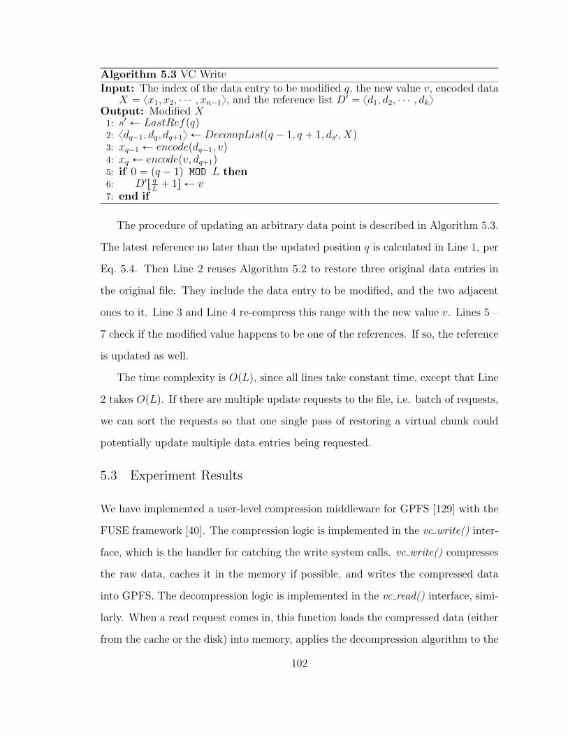
Algorithm 5.3 VC Write

Input: The index of the data entry to be modified q, the new value v, encoded dataX “ xx1, x2, ¨ ¨ ¨ , xn´1y, and the reference list D1 “ xd1, d2, ¨ ¨ ¨ , dky

Output: Modified X1: s1 Ð LastRefpqq2: xdq´1, dq, dq`1y Ð DecompListpq ´ 1, q ` 1, ds1 , Xq3: xq´1 Ð encodepdq´1, vq4: xq Ð encodepv, dq`1q5: if 0 “ pq ´ 1q MOD L then6: D1r q

L` 1s Ð v

7: end if

The procedure of updating an arbitrary data point is described in Algorithm 5.3.

The latest reference no later than the updated position q is calculated in Line 1, per

Eq. 5.4. Then Line 2 reuses Algorithm 5.2 to restore three original data entries in

the original file. They include the data entry to be modified, and the two adjacent

ones to it. Line 3 and Line 4 re-compress this range with the new value v. Lines 5 –

7 check if the modified value happens to be one of the references. If so, the reference

is updated as well.

The time complexity is OpLq, since all lines take constant time, except that Line

2 takes OpLq. If there are multiple update requests to the file, i.e. batch of requests,

we can sort the requests so that one single pass of restoring a virtual chunk could

potentially update multiple data entries being requested.


We have implemented a user-level compression middleware for GPFS [129] with the

FUSE framework [40]. The compression logic is implemented in the vc write() inter-

face, which is the handler for catching the write system calls. vc write() compresses

the raw data, caches it in the memory if possible, and writes the compressed data

into GPFS. The decompression logic is implemented in the vc read() interface, simi-

larly. When a read request comes in, this function loads the compressed data (either

from the cache or the disk) into memory, applies the decompression algorithm to the

102

compressed data, and passes the result to the end users.

The virtual chunk middleware is deployed on each compute node as a mount

point that refers to the remote GPFS file system. This architecture enables a high

possibility of reusing the decompressed data, since the decompressed data are cached

in the local node. Moreover, because the original compressed file is split into many

logical chunks each of which can be decompressed independently, it allows a more

flexible memory caching mechanism and parallel processing of these logical chunks.

We have implemented a LRU replacement policy for caching the intermediate data.

We have also integrated virtual chunks into the FusionFS [172] distributed file

system. The key feature of FusionFS is to fully exploit the available resources and

avoid any centralized component. That is, each participating node plays three roles

at the same time: client, metadata server, and data server. Each node is able to pull

the global view of all the available files by the single namespace implemented with

a distributed hash table [73], even though the metadata is physically distributed on

all the nodes. Each node stores parts of the entire metadata and data at its local

storage. Although both metadata and data are fully distributed on all nodes, the

local metadata and data on the same node are completely decoupled: the local data

may or may not be described by the local metadata. By decoupling metadata and

data, we are able to apply flexible strategies on metadata management and data

I/Os.

On each compute node, a virtual chunk component is deployed on top of the

data I/O implementation in FusionFS. FusionFS itself has employed FUSE to sup-

port POSIX, so there is no need for VC to implement FUSE interfaces again. In-

stead, VC is implemented in the fusionfs write() and the fusionfs read() interfaces.

Although the compression is implemented in the fusionfs write() interface, the com-

pressed file is not persisted into the hard disk until the file is closed. This approach

can aggregate the small blocks into larger ones, and reduce the number of I/Os to

103

improve the end-to-end time. In some scenarios, users are more concerned for the

high availability rather than the compressing time. In that case, a fsync() could be

called to the (partially) compressed data to ensure these data are available at the

persistent storage in a timely manner, so that other processes or nodes could start

processing them.

The remainder of this section answers the following questions:

1. How does the number of VC affect the compression ratio and sequential I/O

time (§5.3.1)?

2. How does VC, as a middleware, improve the GPFS [129] I/O throughput

(§5.3.2)?

3. How does VC, as a built-in component, help to improve the I/O throughput

of FusionFS [172] (§5.3.3)?

All experiments were repeated at least five times, or until results became stable

(i.e. within 5% margin of error); the reported numbers are the average of all runs.

5.3.1 Compression Ratio

We show how virtual chunks affect the compression ratio on the Global Cloud Re-

solving Model (GCRM) data [41]. GCRM consists of single-precision float data of

temperatures to analyze cloud’s influence on the atmosphere and the global climate.

In our experiment there are totally n “ 3.2 million data entries to be compressed

with the aforementioned XOR compressor. Each data entry comprises a row of 80

single-precision floats. Note that based on our previous analysis in §5.2.3, the op-

timal number of references should be set roughly to?n « 1, 789 (Eq. 5.3, §5.2.3).

Thus we tested up to 2,000 references, a bit more than the theoretical optimum.

From 1 to 2,000 references, the compression ratio change is reported in Table 5.2,

together with the overall wall time of the compression. As expected, the compres-

104

Table 5.2: Overhead of additional references

Number ofReferences

CompressionRatio

Wall Time(second)

1 1.4929 415.40400 1.4926 415.47800 1.4923 415.541200 1.4921 415.621600 1.4918 415.692000 1.4915 415.76

sion ratio decreases when more references are appended. However, the degradation

of compression ratio is almost negligible: within 0.002 between 1 reference and 2000

references. These small changes to the compression ratios then imply negligible differ-

ences of the wall time also: within sub-seconds out of minutes. Thus, this experiment

demonstrates that adding a reasonable number of additional references, guided by

the analysis in §5.2.3, only introduces negligible overhead to the compression process.

The reason of the negligible overhead is in fact due to Eq. 5.2, or Eq. 5.3 as

a simplified version discussed in §5.2.3. The total number of data entries is about

quadratic to the optimal number of references, making the cost of processing the

additional references only marginal to the overall compression procedure, particularly

when the data size is large.

5.3.2 GPFS Middleware

We deployed the virtual chunk middleware on 1,024 cores (256 physical nodes) point-

ing to a 128-nodes GPFS [129] file system on Intrepid [58], an IBM Blue Gene/P

supercomputer at Argonne National Laboratory. Each Intrepid compute node has

a quad-core PowerPC 450 processor (850MHz) and 2GB of RAM. The dataset is

244.25GB of the GCRM [41] climate data.

Since virtual chunk is implemented with FUSE [40] that adds extra context

switches when making I/O system calls, we need to know how much overhead is

105

induced by FUSE. To measure the impact of this overhead, the GCRM dataset is

written to the original GPFS and the GPFS+FUSE file system (without virtual

chunks), respectively. The difference is within 2.2%, which could be best explained

by the fact that in parallel file systems the bottleneck is on the networking rather

than the latency and bandwidth of the local disks. Since the FUSE overhead on

GPFS is smaller than 5%, we will not distinguish both setups (original GPFS and

FUSE+GPFS) in the following discussion.

We tested the virtual chunk middleware on GPFS with two routine workloads:

(1) the archival (i.e. write with compression) of all the available data; and (2) the

retrieval (i.e. read with decompression) of the latest temperature, regarded as the

worst-case scenario discussed in §5.2.3. The I/O time, as well as the speedup over

the baseline of single-reference compression, is reported in Figure 5.2(a). We observe

that multiple references (400 – 2000) significantly reduce the original I/O time from

501s to 383s, and reach the peak performance at 800-references with 31% (1.3X)

improvement.

An interesting observation from Figure 5.2(a) is that, the performance sensitiv-

ity to the number of references near the optimal kopt is relatively low. The optimal

number of references seems to be 800 (the shortest time: 383.35 seconds), but the

difference across 400-2000 references is marginal, only within sub-seconds. This phe-

nomenon is because that beyond a few hundreds of references, the GCRM data set

has reached a fine enough granularity of virtual chunks that could be efficiently de-

compressed. To justify this, we re-run the experiment with finer granularity from 1

to 200 references as reported in Figure 5.2(b). As expected, the improvement over

1–200 references is more significant than between 400 and 2000. This experiment

also indicates that, we could achieve a near-optimal (within 1%) performance (30.0%

speedup at k “ 50 vs 30.70% at k “ 800) with only 50800“ 6.25% cost of additional

references. It thus implies that even fewer references than?n could become signifi-

106

(a) Coarse Granularity 1 – 2000

(b) Fine Granularity 1 – 200

Figure 5.2: I/O time with virtual chunks in GPFS

cantly beneficial to the overall I/O performance.

To study the effect of virtual-chunk compression to real applications, we ran the

MMAT application [11] that calculates the minimal, maximal, and average tem-

peratures on the GCRM dataset. The breakdown of different portions is shown in

Figure 5.3. Indeed, MMAT is a data-intensive application, as this is the application

107

type where data compression is useful. So we can see that in vanilla GPFS 97%

(176.13 out of 180.97 seconds) of the total runtime is on I/O. After applying the

compression layer (k “ 800), the I/O portion is significantly reduced from 176.13 to

118.02 seconds. Certainly this I/O improvement is not free, as there is 23.59 seconds

overhead for the VC computation. The point is, this I/O time saving (i.e. 176.13

- 118.02 = 58.11 seconds) outweighs the VC overhead (23.59 seconds), resulting in

1.24X speedup on the overall execution time.

Figure 5.3: Execution time of the MMAT application

5.3.3 FusionFS Integration

We have deployed FusionFS integrated with virtual chunks to a 64-nodes Linux

cluster at Illinois Institute of Technology. Each node has two Quad-Core AMD

Opteron 2.3GHz processors with 8GB RAM and 1TB Seagate Barracuda hard drive.

All nodes are interconnected with a 1Gbps Ethernet. Besides the GCRM [41] data,

we also evaluated another popular data set Sloan Digital Sky Survey (SDSS [131])

that comprises a collection of astronomical data such as positions and brightness of

hundreds of millions of celestial objects.

We illustrate how virtual chunks help FusionFS to improve the I/O throughput

108

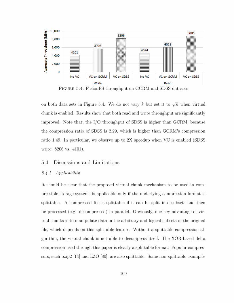
Figure 5.4: FusionFS throughput on GCRM and SDSS datasets

on both data sets in Figure 5.4. We do not vary k but set it to?n when virtual

chunk is enabled. Results show that both read and write throughput are significantly

improved. Note that, the I/O throughput of SDSS is higher than GCRM, because

the compression ratio of SDSS is 2.29, which is higher than GCRM’s compression

ratio 1.49. In particular, we observe up to 2X speedup when VC is enabled (SDSS

write: 8206 vs. 4101).

5.4 Discussions and Limitations

5.4.1 Applicability

It should be clear that the proposed virtual chunk mechanism to be used in com-

pressible storage systems is applicable only if the underlying compression format is

splittable. A compressed file is splittable if it can be split into subsets and then

be processed (e.g. decompressed) in parallel. Obviously, one key advantage of vir-

tual chunks is to manipulate data in the arbitrary and logical subsets of the original

file, which depends on this splittable feature. Without a splittable compression al-

gorithm, the virtual chunk is not able to decompress itself. The XOR-based delta

compression used through this paper is clearly a splittable format. Popular compres-

sors, such bzip2 [14] and LZO [80], are also splittable. Some non-splittable examples

109

include Gzip [52] and Snappy [135].

It should also be noted that virtual chunks are not designed for general-purpose

compression, but for highly compressible scientific data. This is why this study did

not evaluate a virtual chunk version of general compressors (e.g. bzip2, LZO), since

they are not designed for numerical data used in scientific applications.

5.4.2 Dynamic Virtual Chunks

If the access pattern does not follow the uniform distribution, and this information

is exposed to users, then it makes sense to specify more references (i.e. finer gran-

ularity of virtual chunks) for the subset that is more frequently accessed. This is

because more references make random accesses more efficiently with a shorter dis-

tance (and less computation) from the closest reference, in general. The assumption

of equidistant reference, thus, would not hold any more in this case.

One intuitive solution to adjust the virtual chunk granularity is to ask users to

specify where and how to update the reference. It implies that the users are expected

to have a good understanding of their applications, such as I/O patterns. This is a

reasonable assumption in some cases, for example if the application developers are

the main users. Therefore, we expect that the users would specify the distribution

of the reference density in a configuration file, or more likely a rule such as a decay

function [24].

Nevertheless we believe it would be more desirable to have an autonomic mech-

anism to adjust the virtual chunks for those domain users without the technical

expertise such as chemists, astronomers, and so on. This remains an open question

to the community and a direction of our future work.

110

5.4.3 Data Insertion and Data Removal

We are not aware of much need for data insertion and data removal within a file

in the context of HPC or scientific applications. By insertion, we mean a new data

entry needs to be inserted into an arbitrary position of an existing compressed file.

Similarly, by removal we mean an existing value at an arbitrary position needs to

be removed. Nevertheless, it would make this work more complete if we supported

efficient data insertion and data removal when enabling virtual chunks in storage

compression.

A straightforward means to support this operation might treat a data removal as

a special case of data writes with the new value as null. But then it would bring new

challenges such as dealing with the “holes” within the file. We do not think either

is a trivial problem, and would like to have more discussions with HPC researchers

and domain scientists before investing in such features.

5.5 Summary

Conventional file- and block-level storage compression have shown their limits for sci-

entific applications: file-level compression provides little support for random access,

and block-level compression significantly degenerates the overall compression ratio

due to the per-block compression overhead. This chapter introduces virtual chunks

to support efficient random accesses to compressed scientific data while retaining the

high compression ratio. Virtual chunks keep files’ physical entirety, because they are

referenced by pointers beyond the file end. The physical entirety helps to achieve a

high compression ratio by avoiding the per-block compression overhead. The addi-

tional references take insignificant storage space and add negligible end-to-end I/O

overhead. Virtual chunks enable efficient random accesses to arbitrary positions of

the compressed data without decompressing the whole file. Procedures for manipu-

111

lating virtual chunks are formulated, along with the analysis of optimal parameter

setup. Evaluation demonstrates that virtual chunks improve scientific applications’

I/O throughput by up to 2X speedup at large scale.

112

6

Filesystem Reliability through Erasure Coding

This chapter investigates if GPU technologies can speedup erasure coding to replace

conventional file replication. Erasure coding offers high data reliability with less

space, as it does not require full replicas but only smaller parities. The major cri-

tique for erasure coding, however, lies on its computational overhead, because the

encoding and decoding process used to be extremely slow on conventional CPUs due

to complex matrix computations. Nevertheless, today’s GPUs are architected with

massively concurrent computing cores that are good at SIMD applications such as

matrix computations. To justify the feasibility of GPU-accelerated erasure coding,

we build a GPU-accelerated erasure-coding-based distributed key-value store (Gest)

from the ground up. Preliminary results were published in [170]. Experiment results

show that Gest, when properly configured, achieves the same level of reliability as

data replication, but with significantly higher space efficiency and I/O performance.

113

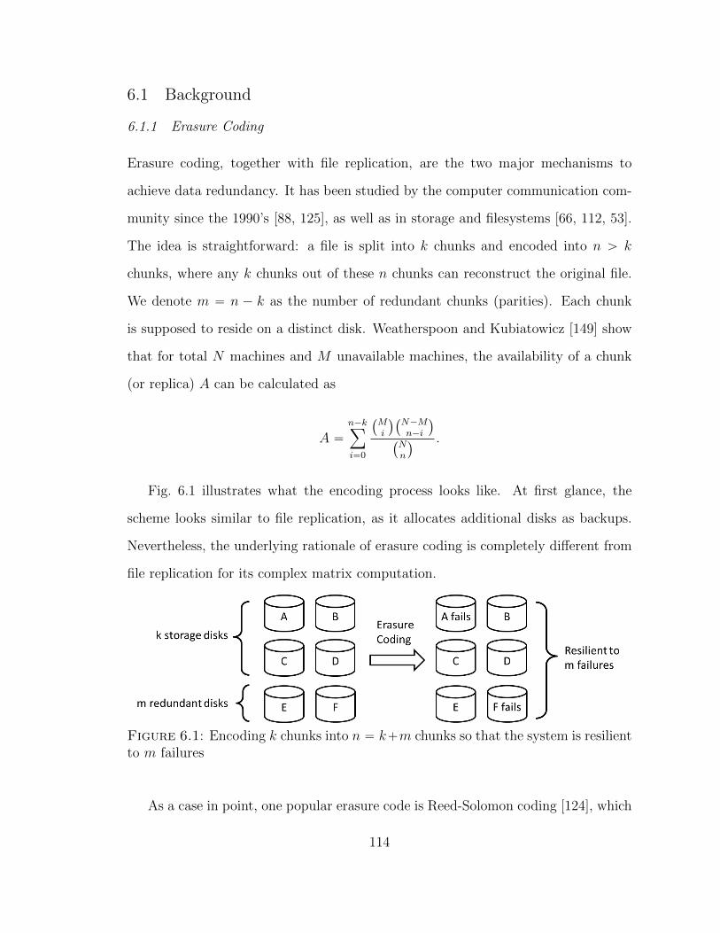
6.1 Background

6.1.1 Erasure Coding

Erasure coding, together with file replication, are the two major mechanisms to

achieve data redundancy. It has been studied by the computer communication com-

munity since the 1990’s [88, 125], as well as in storage and filesystems [66, 112, 53].

The idea is straightforward: a file is split into k chunks and encoded into n ą k

chunks, where any k chunks out of these n chunks can reconstruct the original file.

We denote m “ n ´ k as the number of redundant chunks (parities). Each chunk

is supposed to reside on a distinct disk. Weatherspoon and Kubiatowicz [149] show

that for total N machines and M unavailable machines, the availability of a chunk

(or replica) A can be calculated as

A “n´kÿ

i“0

`

Mi

˘`

N´Mn´i

˘

`

Nn

˘ .

Fig. 6.1 illustrates what the encoding process looks like. At first glance, the

scheme looks similar to file replication, as it allocates additional disks as backups.

Nevertheless, the underlying rationale of erasure coding is completely different from

file replication for its complex matrix computation.

Figure 6.1: Encoding k chunks into n “ k`m chunks so that the system is resilientto m failures

As a case in point, one popular erasure code is Reed-Solomon coding [124], which

114

uses a generator matrix built from a Vandermonde matrix to multiply the k data to

get the encoded k `m codewords, as shown in Fig. 6.2.

Figure 6.2: Encoding 4 files into 6 codewords with Reed-Solomon coding

Comparing with data replication, erasure coding has 3 important features.

First, erasure coding offers higher space efficiency, defined as kn. This is because

redundant parities are smaller than the file itself. Tanenbaum and Steen [139] report

that erasure coding outperforms data replication by 40% - 200% in terms of space

efficiency.

Second, erasure coding consumes less network bandwidth, because we need not

send the entire files but only fractions of them (i.e. parities). This feature is critical

in limited network resources, e.g. geographically dispersed Internet-connected Cloud

computing systems built with commodity hardware.

The last and often underrated advantage is security. Rather than copying the

intact and non-encrypted file from one node to another, erasure coding chops the

file into chunks, then encodes and disperses them to remote nodes. This process is

115

hard to reverse if the encoding matrix is wisely chosen. Moreover, erasure coding-

based data redundancy guarantees data security with pk ´ 1q compromised nodes

because the minimal number of chunks to restore the original file is k. In contrast,

a simple file replication cannot tolerate any compromised nodes; if one node (with

the replica) is compromised, the entire file is immediately compromised. Therefore,

for applications with sensitive data, erasure coding is the preferred mechanism over

replication.

The drawback of erasure coding stems from its computation overhead. It places

an extensive burden on the computing chips, so it used to be impractical for produc-

tion storage systems. This is one of the reasons why prevailing distributed storage

systems (e.g. Hadoop distributed file system [134], Google file system [44]) prefer

data replication to erasure codes.

6.1.2 GPU Computing

The graphics processing unit (GPU) was originally designed to rapidly process images

for the display. The nature of image manipulations on displays differs from tasks

typically performed by the CPU. Most image operations are conducted with single

instruction and multiple data (SIMD), where a general-purpose application on a CPU

takes multiple instructions and multiple data (MIMD). To meet the requirement of

computer graphics, GPU is designed to have many more cores on a single chip than

CPU, all of which carry out the same instructions at the same time.

The attempt to leverage GPU’s massive number of computing units can be

tracked back to the 1970’s in [61]. GPUs, however, did not become popular for

processing general applications due to its poor programmability until GPU-specific

programming languages and frameworks were introduced such as OpenCL [138] and

CUDA [102]. These tools greatly eased the development of general applications run-

ning on GPUs, thus opened the door to improving applications’ performance with

116

GPU acceleration, which are usually named general-purpose computing on graph-

ics processing units (GPGPU). GPGPU gains tremendous research interest because

of the huge potential to improve the performance by exploiting the parallelism of

GPU’s many-core architecture as well as GPU’s relatively low power consumption,

as shown in [161, 21, 78].

Table 6.1 shows a comparison between two mainstream GPU and CPU devices,

which will also be used in the testbeds for evaluation later in this paper. Although the

GPU frequency is only about 50% of CPU, the amount of cores outnumbers CPU by

3366“ 66X. So the overall computing capacity of GPU is still more than one order of

magnitude higher than CPU. This GPU’s power consumption should also be noted;

only 0.4820.83

“ 2.3% of CPU. As energy cost is one of the most challenging problems

in large-scale storage systems [127, 63, 168, 167, 159], GPU has the potential to

ameliorate it.

Table 6.1: Comparisons of two mainstream GPU and CPU

Device Nvidia GTX460 AMD Phenom

Number of Cores 336 6Frequency (GHz) 1.56 3.3Power (W / core) 0.48 20.83

6.2 Gest Distributed Key-Value Storage

Cloud platforms such as Microsoft Azure [91] and Amazon EC2 [5] usually provide a

simple yet versatile hashtable-like API (e.g. set(key,value), value Ð get(key))

to its underlying distributed storage. The hashtable API relaxes the conventional

POSIX API, simplifies otherwise complicated file operations, enables a unified I/O

interface to a large variety of applications, thus gains increasing popularity. The

storage subsystems underneath these Cloud platforms are typically implemented as

distributed key-value stores, which, despite slight implementation differences, assign

117

the file name as the key and the file content (or, blob) as the value.

The state-of-the-art approach for distributed key-value stores to achieve reliability

is replication: several remote replicas are created and updated when the primary copy

is touched. Redundant file replicas, however, cause the following issues: (1) space

overhead, (2) additional (local) disk I/O, and (3) network bandwidth consumption.

As a case in point, if every file has two replicas, the space overhead is roughly 200%,

along with tripled disk I/O and network traffic.

This chapter, from a system’s perspective, seeks the answer to this burning ques-

tion: how to efficiently achieve key-value store’s data reliability with affordable over-

head from the space, I/O, and network? Rather than proposing a new algorithm or

model [156, 155], this work is orthogonal to previous study in that we build a real

distributed key-value storage system from the ground up with the following design

principles: (1) naive file-level replication need to be replaced by more space-efficient

mechanisms, and (2) I/O-intensive operations, if possible, should be transformed

to compute-intensive ones without affecting the results. While the first principle is

self-explanatory, the second one is because modern computer’s computing capacity

is orders of magnitude faster than its I/O.

A bird’s view of Gest architecture is shown in Fig. 6.3. Two services are installed

on each Gest node: metadata management and data transfer. Each instance of these

two services on a particular node communicates to other peers over the network when

requested metadata or files cannot be found on the local node.

To make matters more concrete, Fig. 6.4 illustrates the scenario when writing

and reading a file for k “ 4 and m “ 2. On the left hand side when the original

file (i.e. orig.file) is written, the file is chopped into k “ 4 chunks and encoded

into n “ k ` m “ 6 chunks. These 6 chunks are then dispersed into 6 different

nodes after which their metadata are sent to the metadata hashtable, which is also

physically distributed across these 6 nodes. A file read request (on the right hand

118

Figure 6.3: Architectural overview of Gest deployed on an n-nodes distributedsystem. End users run applications on the ith node where files are encoded anddecoded by erasure algorithms.

side) is essentially the reversed procedure of a file write: retrieves the metadata,

transfers the chunks, and decodes the file.

Figure 6.4: An example of file writing and reading on Gest

119

6.2.1 Metadata Management

The traditional way of handling metadata for distributed systems is to manipulate

them on one or a few nodes. The rational is that metadata contains only high level

information (small in size), so a centralized repository usually meets the requirement.

Most production distributed storage systems employ centralized metadata manage-

ment, for instance the Google file system [44] keeps all its metadata on the master

node. This design is easy to implement and maintain, yet exposes a performance

bottleneck for the workloads generating a large amount of small files: the metadata

rate from a great number of small files can easily saturate the limited number of

metadata servers.

In contrast, we implement Gest’s metadata management system in a completely

distributed fashion. Specifically, all meatdata are dispersed into a distributed hashtable

(ZHT [73]). While there are multiple choices of distributed hashtable implementa-

tions such as Memcached [36] and Dynamo [28], ZHT has some features that are

crucial to the success of serving as a metadata manager.

In Gest, clients have a coherent view of all the files (i.e. metadata) no matter

if the file is stored in the local node or a remote node. That is, a client interacts

with Gest to inquiry any file on any node. This implies that applications are highly

portable across Gest nodes and can run without modifications or recompiling. The

metadata and data on the same node, however, are completely decoupled: a file’s

location has nothing to do with its metadata’s location.

Besides the conventional metadata information for regular files, there is a special

flag to indicate if this file is being written. Specifically, any client who requests to

write a file needs to acquire this flag before opening the file, and will not reset it until

the file is closed. The atomic compare-swap operation supported by ZHT guarantees

file’s consistency for concurrent writes.

120

6.2.2 Erasure Libraries

Besides daemon services running at the back end, Gest plugs in encoding and decod-

ing modules on the fly. Plank et al. [112] make a thorough review of erasure libraries.

In this early version of Gest, we support two built-in libraries Jerasure [110] and

Gibraltar [25] as the default CPU and GPU libraries, respectively. Gest is imple-

mented to be flexible enough to support more libraries.

Jerasure is a C/C++ library that supports a wide range of erasure codes: Reed-

Solomon coding, Minimal Density RAID-6 coding, Cauchy Reed-Solomon coding,

and most generator matrix coding. One of the most popular codes is the Reed-

Solomon encoding method, which has been used for the RAID-6 disk array model.

This coding can either use Vandermonde or Cauchy matrices to create generator

matrices.

Gibraltar is a Reed-Solomon coding library for storage applications. It has been

demonstrated to be highly efficient when tested in a prototype RAID system. This

library is known to be more flexible than other RAID standards; it is scalable with

parity’s size of an array. Gibraltar has been created in C using Nvidia’s CUDA

framework.

6.2.3 Workflows

When an application writes a file, Gest splits the file into k chunks. Depending

on which coding library the user chooses to use, these k chunks are encoded into

n “ k `m chunks, which are sent to n different nodes by GDT.

At this point the data migration is complete, and we will need to update the

metadata information. To do so, ZHT on each of these n nodes is pinged to update

the file entries. This procedure of metadata update on the local node is conducted

by an in-memory hashmap whose contents are asynchronously persisted to the local

disk.

121

Reading a file is just the reversed procedure of writing. Gest retrieves the meta-

data from ZHT and uses GDT to transfer (any) k chunks of data to the node where

the user makes the request. These k chunks are then decoded by the user-specified

library and restored into the original file.

6.2.4 Pipeline

Because the encoded data are buffered, GDT can disperse n encoded chunks onto

n different nodes while the file chunks are still being encoded. This pipeline with

the two levels of encoding and sending allows for combining the two costs instead of

summing them, as described in Fig. 6.5.

Figure 6.5: Pipelining of encoding and transferring for a write operation in Gest

6.2.5 Client API

Gest provides a completely customizable set of parameters for the applications to

tune how Gest behaves. In particular, users can specify which coding library to use,

the number of chunks to split the file (i.e. k), the number of parity chunks (i.e.

m “ n´ k), the buffer size (default is 1MB), and the like.

6.3 Erasure Coding in FusionFS

Erasure coding is applied to the primary copy as soon as the file is closed. This

method avoids the block-level synchronization, and operates before the potential

I/O bottleneck of the underlying persistent storage. In FusionFS, erasure coding

122

logic is implemented in the fusion releasepq interface, which is exactly the point

right after a file is closed but before it is flushed to the disk. As long as the file is

closed (and still in memory), this file is considered “complete”, and is ready to be

split into n chunks by the erasure libraries. These n chunks are then transferred to

n different physical nodes.

6.4 Evaluation

6.4.1 Experiment Design

We compare the conventional file replication to erasure coding mechanisms of differ-

ent parameter combinations at different scales. The list of candidate mechanisms is

summarized in Table 6.2, along with the number of chunks for both the original file

and the redundant data.

Table 6.2: List of data redundancy mechanisms considered in Gest

Mechanism Chunks of Chunks ofName Original File Redundant data

Replica 1 2Erasure1 3 5Erasure2 5 3Erasure3 11 5Erasure4 13 3Erasure5 27 5Erasure6 29 3

For file replication, the “chunks of the original data” is the file itself, and the

“chunks of redundant data” are plain copies of the original file. We choose 2 replicas

for file replication as the baseline, since this is the default setup of most existing

systems. Therefore we see <Replica, 1, 2> in Table 6.2.

Similarly, Gest with different erasure-coding parameters are listed as Erasure[1..6],

along with different file granularity and additional parities. We design experiments

at different scales to show how Gest scales. Specifically, every pair of erasure mech-

123

anisms represents a different scale: Erasure[1,2] for 8-nodes, Erasure[3,4] for

16-nodes, and Erasure[5,6] for 32-nodes. For example, tuple <Erasure6, 29, 3>

says that we split the original file into 29 chunks, encode them with 3 additional

parities, and send out the total 32 chunks into 32 nodes.

The numbers of redundant parities (i.e. “chunks of redundant data”) for Erasure[1..6]

are not randomly picked, but in accordance with the following two rules. First, we are

only interested in those erasure mechanisms that are more reliable than the replica-

tion baseline, because our goal is to build a more space-efficient and faster key-value

store without compromised reliability. Therefore in all erasure cases, there are at

least 3 redundant parities, which are more than the replica case (i.e. 2). Second,

we want to show how different levels of reliability affect the space efficiency and I/O

performance. So there is one additional configuration for each scale: the redundant

parities are increased from 3 to 5.

6.4.2 Data Reliability and Space Efficiency

Fig. 6.6 shows the tolerable failures (i.e. data reliability) and space efficiency for

each of the 7 mechanisms listed in Table 6.2. The tolerable failures (histograms) of

Erasure[1..6] are all more than Replica, so is the space efficiency. Thus, when

properly configured, erasure codes are better choices than replication in terms of both

reliability and efficiency. Before we investigate more about performance in §6.4.3,

the following conclusions are drawn from Fig. 6.6.

First, a larger scale enables higher space efficiency. This is somewhat counter-

intuitive, as it is a well-accepted practice to collect data to a small subset of nodes

(e.g. collective I/O buffers small and dispersed I/O to reduce the number of small

I/Os). Fig. 6.6, however, demonstrates that when redundant parity stays the same,

space efficiency is monotonic increasing on more nodes. The reason is that with more

nodes the redundant parity is in finer granularity and smaller in size. Therefore less

124

Figure 6.6: Data reliability and space efficiency

space is taken by the redundant data.

Second, for a specific erasure code at a particular scale, reliability and efficiency

are negatively correlated. For example, if we increase tolerable failures from 3 to 5,

the space efficiency goes from 65% down to 35% (i.e. Erasure2ÑErasure1). This

is understandable, as increasing parities take more space.

6.4.3 I/O Performance

We compare the read and write throughput of all mechanisms listed in Table 6.2 on

the HEC cluster at 8-nodes, 16-nodes, and 32-nodes scales. The files to be read and

written are 1GB per node, with block size 1MB. The result is reported in Fig. 6.7.

While most numbers are self-explanatory, some need more explanations in the fol-

lowing.

One important observation from Fig. 6.7 is the promising performance by erasure

coding even on CPUs. In many cases (e.g. file read on 16-nodes with Erasure4),

Gest delivers higher throughput than the replication counterpart. This is because

125

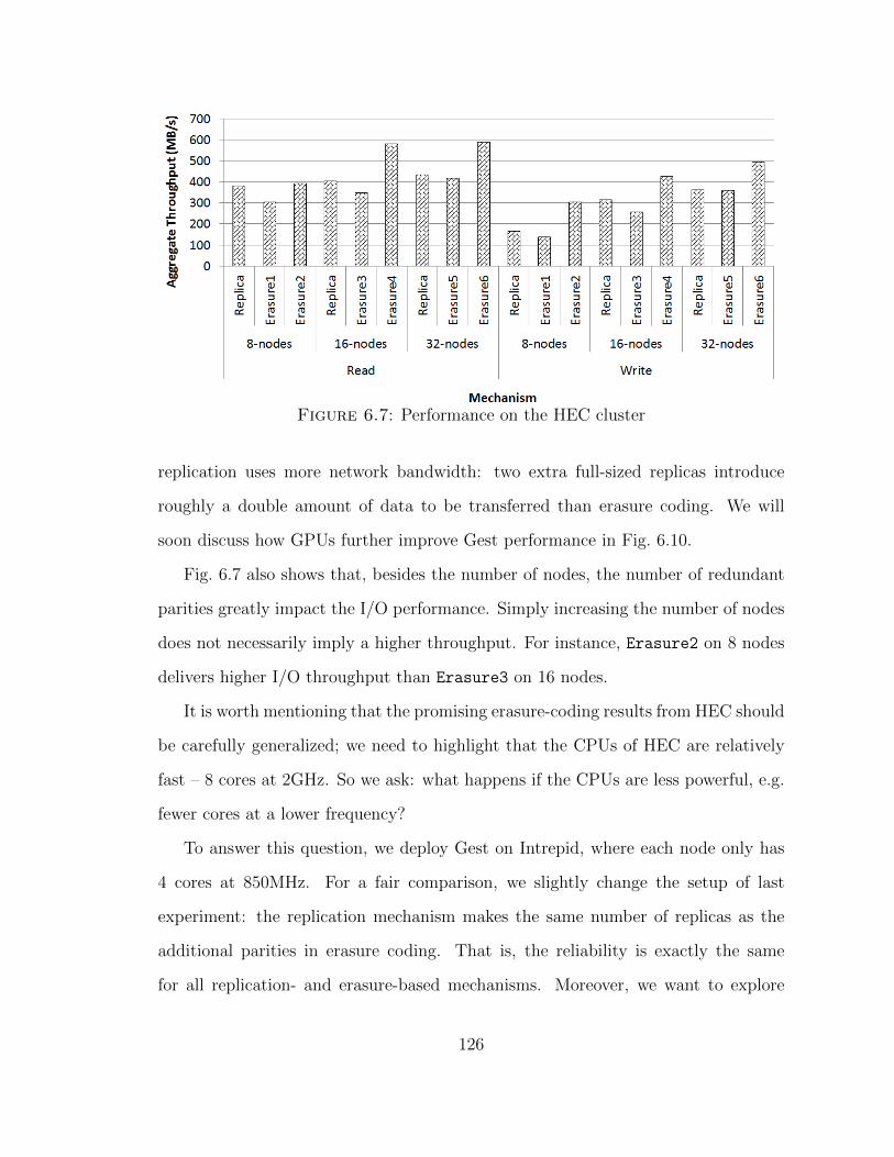
Figure 6.7: Performance on the HEC cluster

replication uses more network bandwidth: two extra full-sized replicas introduce

roughly a double amount of data to be transferred than erasure coding. We will

soon discuss how GPUs further improve Gest performance in Fig. 6.10.

Fig. 6.7 also shows that, besides the number of nodes, the number of redundant

parities greatly impact the I/O performance. Simply increasing the number of nodes

does not necessarily imply a higher throughput. For instance, Erasure2 on 8 nodes

delivers higher I/O throughput than Erasure3 on 16 nodes.

It is worth mentioning that the promising erasure-coding results from HEC should

be carefully generalized; we need to highlight that the CPUs of HEC are relatively

fast – 8 cores at 2GHz. So we ask: what happens if the CPUs are less powerful, e.g.

fewer cores at a lower frequency?

To answer this question, we deploy Gest on Intrepid, where each node only has

4 cores at 850MHz. For a fair comparison, we slightly change the setup of last

experiment: the replication mechanism makes the same number of replicas as the

additional parities in erasure coding. That is, the reliability is exactly the same

for all replication- and erasure-based mechanisms. Moreover, we want to explore

126

the entire parameter space. Due to limited paper space, we only enumerate all the

possible parameter combinations with constraint of 8 total nodes, except for trivial

cases of a single original or redundant chunk. That is, we report the performance

in the following format (file chunks: redundant parities): (2:6), (3:5), (4:4),

(5:3), and (6:2); we are not interested in (1:7) and (7:1), though.

As reported in Fig. 6.8, for all the possible parameters of erasure coding, Gest is

slower than file replication. As a side note, the throughput is orders of magnitude

higher than other testbeds because Intrepid does not have local disk and we run the

experiments on RAM disks. Rather than disappointing, this experiment justifies our

previous conjecture on the importance of computing capacity to the success of Gest.

After all, the result intuitively makes sense; a compute-intensive algorithm needs a

powerful CPU. This, in fact, leads to one purpose of this paper: what if we utilize

even faster chips, e.g. GPUs?

Figure 6.8: Performance on Intrepid

Before discussing the performance of GPU-powered Gest at scales, we investigate

GPU and CPU coding speed on a single Sirius node. As shown in Fig. 6.9, GPU

typically processes the erasure coding one order of magnitude faster than CPU on a

127

variety of block sizes (except for encoding 16MB block size: 6X faster). Therefore,

we expect to significantly reduce the coding time in Gest by GPU acceleration, which

consequently improves the overall end-to-end I/O throughput.

Figure 6.9: Gest coding time on a single Sirius node

We re-run the 8-nodes experiments listed in Table 6.2 on the Sirius cluster. The

number of replicas is set to the same number of redundant parities of erasure coding

for a fair comparison of reliability, just like what we did in Fig. 6.8. The results

are reported in Fig. 6.10, where we see for both (5:3) and (3:5) cases, GPU-powered

erasure coding delivers higher throughput (read and write combined). Recall that

Fig. 6.7 shows that CPU erasure-coding outperforms file replication in some sce-

narios; now Fig. 6.10 says that GPU accelerates erasure-coding to outstrip all the

replication counterparts.

6.4.4 Erasure Coding in FusionFS

Figure 6.11 shows the throughput of erasure coding- and replication-based data re-

dundancy in FusionFS. Only when m “ 2, replication (REP) slightly outperforms

erasure coding (or IDA, information dispersal algorithm), and the difference is al-

128

Figure 6.10: Performance on the Sirius cluster

most negligible. Starting from m “ 3, IDA clearly shows its advantage over REP,

and the speedup increases for the larger m. Particularly, when m “ 6, i.e. to keep

the system’s integrity allowing 6 failed nodes, IDA throughput is 1.82 higher than

the traditional REP method.

Figure 6.11: Throughput of erasure coding and file replication on FusionFS (blocksize 1MB)

We just showed that in FusionFS installed with a commodity GPU, IDA out-

performs REP in terms of both performance and storage utilization (except for the

edge case m “ 2, where IDA and REP are comparable). We believe a high-end GPU

129

would cause a larger gap, and make IDA the top candidate for data redundancy.

6.5 Summary

This chapter presents Gest, a distributed key-value store whose reliability is based on

erasure coding accelerated by GPUs. To the best of our knowledge, Gest is the first

distributed key-value store with built-in erasure coding and GPU acceleration. We,

from a system’s perspective, showcase how to architect and engineer a practical sys-

tem to solve the long-exiting dilemma between data reliability, space efficiency, and

I/O performance. In particular, Gest justifies that key-value stores’ reliability can

be achieved as the same level as conventional file replication but with superior space

efficiency and I/O performance. In a more general sense, Gest demonstrates that

a data-intensive problem can be transformed into a compute-intensive one (erasure

coding), which is then solved by more powerful computing devices (GPUs). We also

demonstrate how to integrate erasure coding into FusionFS. Experiment shows era-

sure coding is a promising approach for a more space-efficient and faster mechanism

than conventional file replication in POSIX filesystems.

130

7

Lightweight Provenance in Distributed Filesystems

It has become increasingly important to capture and understand the origins and

derivation of data (its provenance). A key issue in evaluating the feasibility of data

provenance is its performance, overheads, and scalability.

In this chapter, we explore the feasibility of a general metadata storage and man-

agement layer for parallel file systems, in which metadata includes both file operations

and provenance metadata. We experimentally investigate the design optimality—

whether provenance metadata should be loosely-coupled or tightly integrated with

a file metadata storage systems. We consider two systems that have applied similar

distributed concepts to metadata management, but focusing singularly on kind of

metadata: (i) FusionFS, which implements a distributed file metadata management

based on distributed hash tables, and (ii) SPADE, which uses a graph database to

store audited provenance data and provides distributed module for querying prove-

nance. Results were published in [133, 176].

131

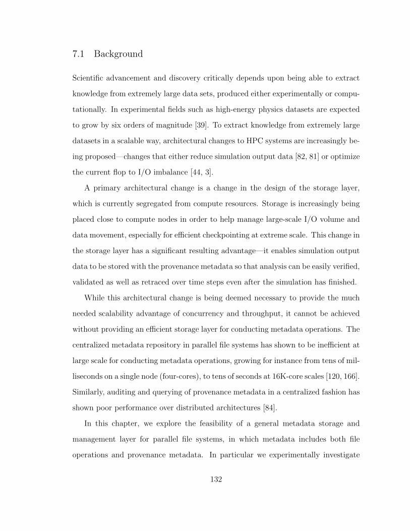
7.1 Background

Scientific advancement and discovery critically depends upon being able to extract

knowledge from extremely large data sets, produced either experimentally or compu-

tationally. In experimental fields such as high-energy physics datasets are expected

to grow by six orders of magnitude [39]. To extract knowledge from extremely large

datasets in a scalable way, architectural changes to HPC systems are increasingly be-

ing proposed—changes that either reduce simulation output data [82, 81] or optimize

the current flop to I/O imbalance [44, 3].

A primary architectural change is a change in the design of the storage layer,

which is currently segregated from compute resources. Storage is increasingly being

placed close to compute nodes in order to help manage large-scale I/O volume and

data movement, especially for efficient checkpointing at extreme scale. This change in

the storage layer has a significant resulting advantage—it enables simulation output

data to be stored with the provenance metadata so that analysis can be easily verified,

validated as well as retraced over time steps even after the simulation has finished.

While this architectural change is being deemed necessary to provide the much

needed scalability advantage of concurrency and throughput, it cannot be achieved

without providing an efficient storage layer for conducting metadata operations. The

centralized metadata repository in parallel file systems has shown to be inefficient at

large scale for conducting metadata operations, growing for instance from tens of mil-

liseconds on a single node (four-cores), to tens of seconds at 16K-core scales [120, 166].

Similarly, auditing and querying of provenance metadata in a centralized fashion has

shown poor performance over distributed architectures [84].

In this chapter, we explore the feasibility of a general metadata storage and

management layer for parallel file systems, in which metadata includes both file

operations and provenance metadata. In particular we experimentally investigate

132

the design optimality—whether provenance metadata should be loosely-coupled or

tightly integrated with a file metadata storage systems. To conduct this experi-

mental evaluation, we consider two systems that have applied similar distributed

concepts to metadata management, but focusing singularly on kind of metadata: (i)

FusionFS [172], which implements a distributed file metadata management based on

distributed hash tables, and (ii) SPADE [42], which uses a graph database to store

audited provenance data and provides distributed module for querying provenance.

Both FusionFS and SPADE are good choices for investigating the metadata stor-

age design problem since both systems have similar manifestation of distributed con-

cepts towards storing their individual metadata: (1) FusionFS provides a POSIX

interface which makes a perfect corresponding for SPADE user-level file system

(FUSE-based) provenance collection; (2) both systems work in a decentralized way

thus actively exploiting the resources at each node.

The remainder of this chapter first introduces the SPADE+FusionFS version of

provenance-aware distributed file system, that aims to offer excellent scalability while

retaining the provenance overhead negligible in traditional clusters. Some prelimi-

nary results of SPADE+FusionFS have been published in [133]. We then investigate

Zero-hop Distributed Hashtable (ZHT) [73] as the underlying storage system for

provenance [176]. ZHT is currently used to store file metadata in FusionFS and pro-

vides the following features that makes it a desirable choice to store provenance: (1)

excellent storage load balancing; (2) light-weighted and fast; (3) excellent scalability;

(4) be able to provide a global view of provenance that aims to provide provenance

capture and management in petascale and exascale. We term the ZHT-backed prove-

nance system as FusionProv.

133

7.2 Local Provenance Middleware

7.2.1 SPADE

SPADE is a software infrastructure for data provenance collection, management, and

analysis. Different operating system level reporters facilitate provenance collection.

The underlying data model is graph-based, consisting of vertices and directed edges,

each of which can be labeled with an arbitrary number of annotations (in the form

of key-value pairs). These annotations can be used to embed the domain-specific

semantics of the provenance. The SPADE system decouples the production, storage,

and utilization of provenance metadata, as illustrated in Figure 7.1. At its core is

a provenance kernel that mediates between the producers and consumers of prove-

nance information, and handles the persistent storage of records. The kernel handles

buffering, filtering, and multiplexing incoming metadata from multiple provenance

sources. It can be configured to commit the elements to multiple databases, and

responds to concurrent queries from local and remote clients.

SPADE Kernel

Query Interface

Storage Interface

Reporter Interface

Consumer Interface

Filters Buffers Mul4plex

Figure 7.1: The SPADE architecture

134

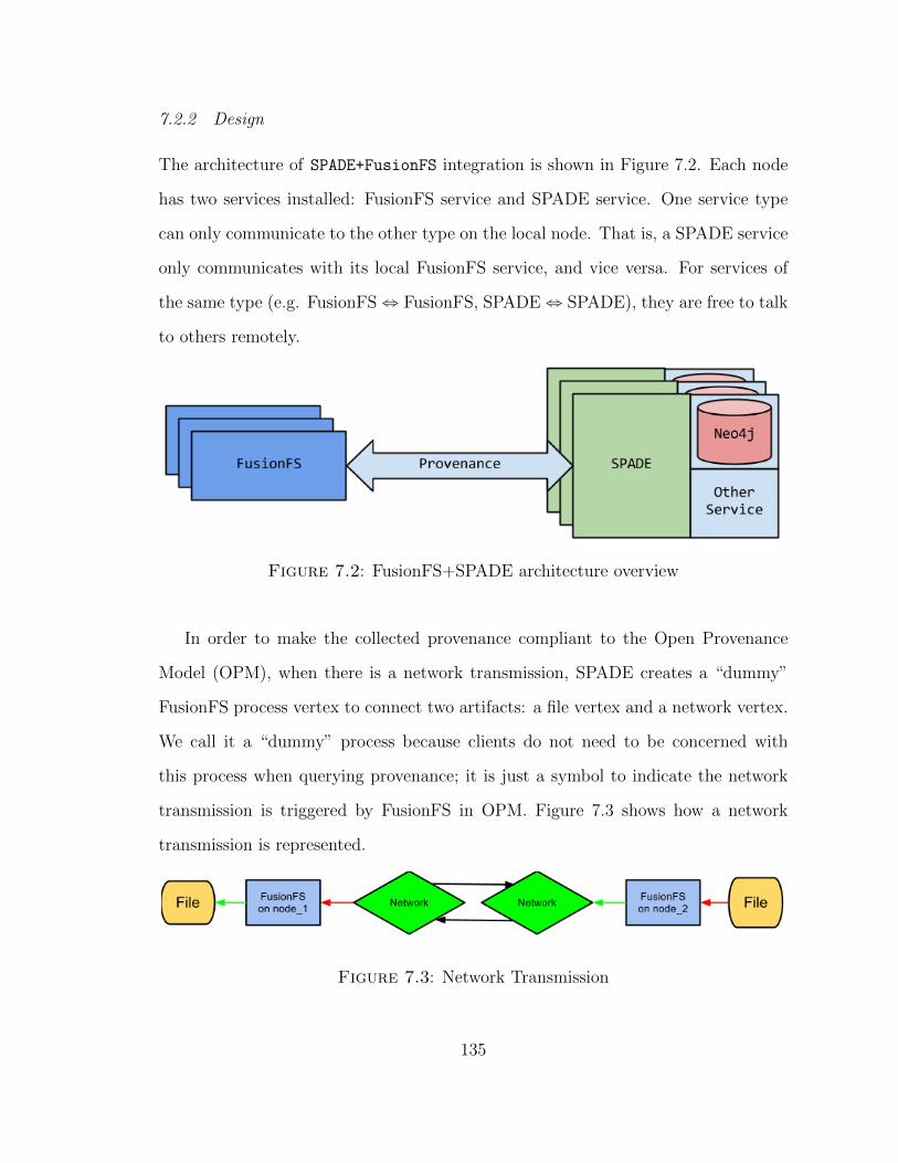
7.2.2 Design

The architecture of SPADE+FusionFS integration is shown in Figure 7.2. Each node

has two services installed: FusionFS service and SPADE service. One service type

can only communicate to the other type on the local node. That is, a SPADE service

only communicates with its local FusionFS service, and vice versa. For services of

the same type (e.g. FusionFS ô FusionFS, SPADE ô SPADE), they are free to talk

to others remotely.

Figure 7.2: FusionFS+SPADE architecture overview

In order to make the collected provenance compliant to the Open Provenance

Model (OPM), when there is a network transmission, SPADE creates a “dummy”

FusionFS process vertex to connect two artifacts: a file vertex and a network vertex.

We call it a “dummy” process because clients do not need to be concerned with

this process when querying provenance; it is just a symbol to indicate the network

transmission is triggered by FusionFS in OPM. Figure 7.3 shows how a network

transmission is represented.

Figure 7.3: Network Transmission

135

7.2.3 Implementation

The key challenge of the proposed work is how to seamlessly integrate SPADE and

FusionFS. All communication between these two services is implemented with TCP.

Asynchronous communication is not used because of the short life cycle of some pro-

cesses. SPADE collects parts of the process information based on system files under

directory /proc/pid. If a process starts and terminates too fast for SPADE to catch,

there would be provenance loss. Therefore it is critical to keep synchronous communi-

cation between SPADE and FusionFS, at least while the two systems are completely

decoupled. We hope to address this in future work with a tighter integration between

FusionFS and SPADE.

Most communication between SPADE and FusionFS consists of simple opera-

tion bindings. For example, FusionFS write operation invokes SPADE to collect

write provenance for this operation. However, as a distributed file system, FusionFS

sometimes needs to migrate files between nodes. The original network provenance

collection in SPADE is not optimized for FusionFS. So we make some customiza-

tion to the network provenance collection to fully hide unnecessary provenance data

outside FusionFS.

7.2.4 Provenance Granularity

One common practice in file manipulations is to split (large) files into blocks to

improve the space efficiency and responsive time. However, for the purpose of prove-

nance, it is less interesting to keep track of file traces at the block level: in most

cases, a file-level provenance would suffice. We have implemented both the file-level

and the block-level provenance tracings, namely, the fine-grained provenance and the

coarse-grained provenance.

136

7.3 Distributed Provenance

7.3.1 Design

Figure 7.4 illustrates how we integrate FusoinFS and ZHT to support distributed

provenance capture at the file system level. Provenance is firstly generated in the

FUSE layer in FusionFS, and then is cached in the local provenance buffer. And at

a certain point (e.g. when the file is closed), the cached provenance will be persisted

into ZHT. Users can do query on any node of the system using a ZHT client.

Figure 7.4: FusionFS+ZHT architecture overview

7.3.2 Implementation

Table 7.1 shows what is captured for the graph vertex in the distributed provenance

store. Basically there are two different vertex types being tracked of: file and pro-

cess. In other words, we are interested in which file(s) have been touched by which

process(es). And we maintain a linked list for the tree topology in ZHT.

We provide a set of APIs to allow users plug their own implementations for the

137

Table 7.1: Attributes of Graph Vertexes in Distributed Provenance Capture

Vertex Type Attributes

File [File path/name] [File version] [File size]Process [Process host] [Process name] [Process command line]

provenance they are interested in. Some commonly used APIs are listed in Table 7.2.

Note that for file creation, there is no need to save the provenance in the local buffers

because it only touches the metadata (rather than the file/process). Therefore this

information is directly stored in the underlying metadata storage (i.e. ZHT).

Table 7.2: Some example APIs available for provenance capture

FusionFS Operation Provenance API

fusion read() prov read()fusion write() prov write()fusion create() prov create()fusion flush() prov push()

We implement a light-weight command-line tool that end users can use to query

the provenance, in the following syntax:

query vertex [file] [version] [ancestors--descendants] [depth]

For example, with a following workflow: a file (origin file) was created by a touch

process on host 12.0.0.1, and later was copied by multiple processes on multiple nodes

(12.0.0.2 to 12.4.0.16). The query on the descendants of the touch process (vertex)

would generate provenance graph showed in Figure 7.5.


We have deployed the distributed provenance-aware file system on 1K-node IBM

BlueGene/P supercomputer Intrepid [58]. We also evaluated both the distributed

and SPADE-extended systems on a 32-node cluster, where each node has two Quad-

Core AMD Opteron 2.3GHz processors with 8GB memory. All nodes are intercon-

138

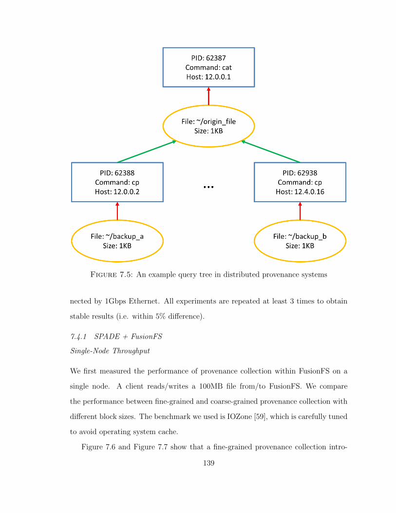
Figure 7.5: An example query tree in distributed provenance systems

nected by 1Gbps Ethernet. All experiments are repeated at least 3 times to obtain

stable results (i.e. within 5% difference).

7.4.1 SPADE + FusionFS

Single-Node Throughput

We first measured the performance of provenance collection within FusionFS on a

single node. A client reads/writes a 100MB file from/to FusionFS. We compare

the performance between fine-grained and coarse-grained provenance collection with

different block sizes. The benchmark we used is IOZone [59], which is carefully tuned

to avoid operating system cache.

Figure 7.6 and Figure 7.7 show that a fine-grained provenance collection intro-

139

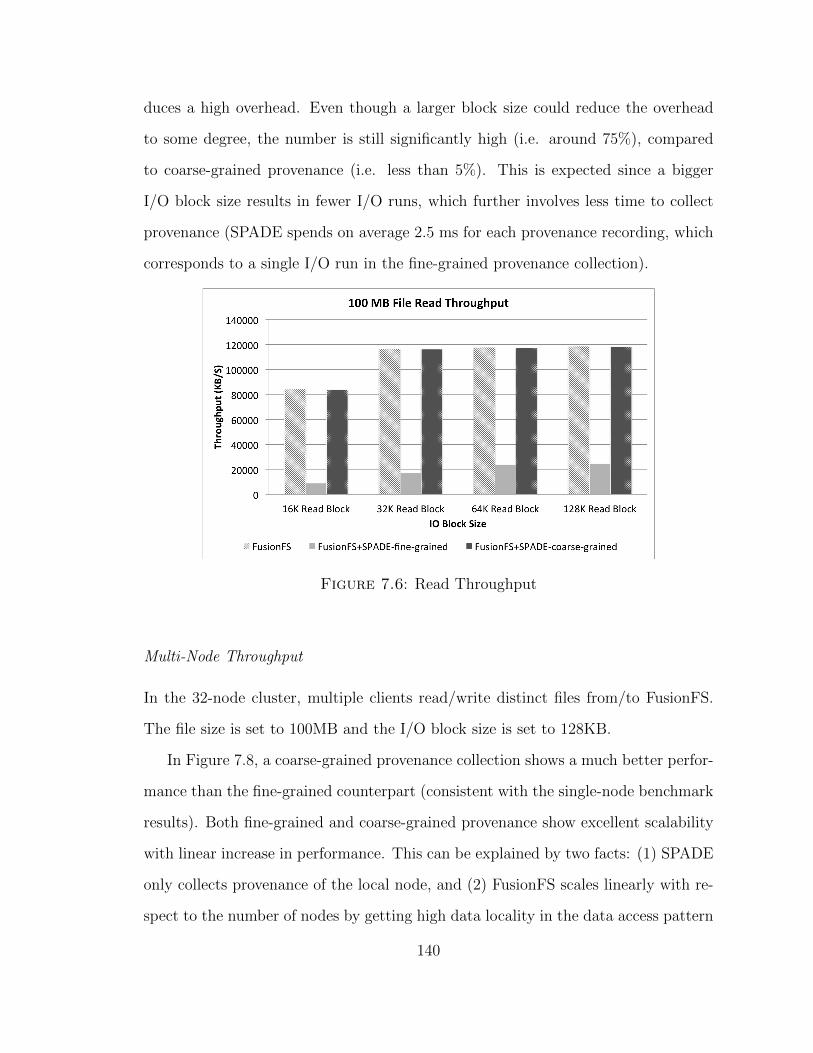
duces a high overhead. Even though a larger block size could reduce the overhead

to some degree, the number is still significantly high (i.e. around 75%), compared

to coarse-grained provenance (i.e. less than 5%). This is expected since a bigger

I/O block size results in fewer I/O runs, which further involves less time to collect

provenance (SPADE spends on average 2.5 ms for each provenance recording, which

corresponds to a single I/O run in the fine-grained provenance collection).

Figure 7.6: Read Throughput

Multi-Node Throughput

In the 32-node cluster, multiple clients read/write distinct files from/to FusionFS.

The file size is set to 100MB and the I/O block size is set to 128KB.

In Figure 7.8, a coarse-grained provenance collection shows a much better perfor-

mance than the fine-grained counterpart (consistent with the single-node benchmark

results). Both fine-grained and coarse-grained provenance show excellent scalability

with linear increase in performance. This can be explained by two facts: (1) SPADE

only collects provenance of the local node, and (2) FusionFS scales linearly with re-

spect to the number of nodes by getting high data locality in the data access pattern

140

Figure 7.7: Write Throughput

evaluated. We have evaluated FusionFS (without SPADE) at scales of up to 1K

nodes on a IBM Blue Gene/P supercomputer with similar excellent results.

Figure 7.8: Multiple-Node 100MB Write Throughtput

Query time

We are interested in the query time of the provenance of a particular file that has

been read by multiple remote nodes. This write-once-read-many is a very frequent

141

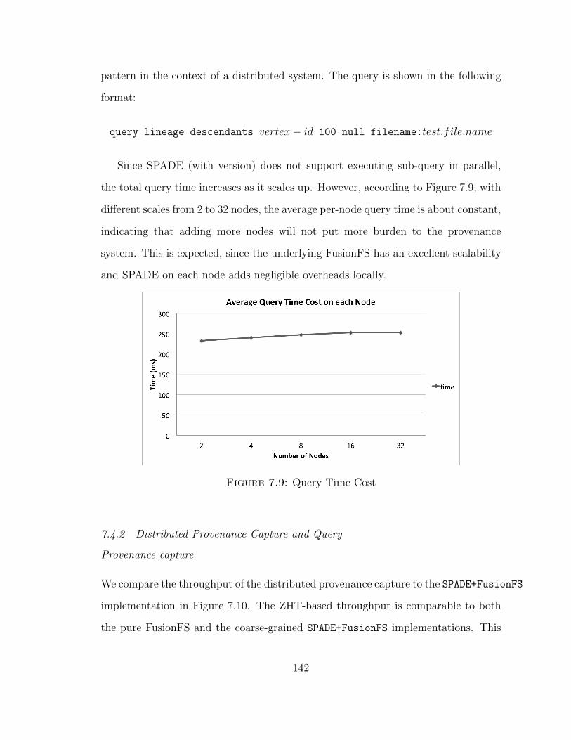
pattern in the context of a distributed system. The query is shown in the following

format:

query lineage descendants vertex´ id 100 null filename:test.file.name

Since SPADE (with version) does not support executing sub-query in parallel,

the total query time increases as it scales up. However, according to Figure 7.9, with

different scales from 2 to 32 nodes, the average per-node query time is about constant,

indicating that adding more nodes will not put more burden to the provenance

system. This is expected, since the underlying FusionFS has an excellent scalability

and SPADE on each node adds negligible overheads locally.

Figure 7.9: Query Time Cost

7.4.2 Distributed Provenance Capture and Query

Provenance capture

We compare the throughput of the distributed provenance capture to the SPADE+FusionFS

implementation in Figure 7.10. The ZHT-based throughput is comparable to both

the pure FusionFS and the coarse-grained SPADE+FusionFS implementations. This

142

result suggests that, even though there is network overhead involved in distributed

provenance capture, the cost is about negligible.

Figure 7.10: Throughput of different implementations of provenance capture

Provenance Query

Similarly to throughput, we also compare the query time of different implementa-

tions. Figure 7.11 shows that even on one single node, the ZHT-based implementa-

tion is much faster than SPADE (0.35ms vs. 5ms). At 32-node scale, the gap is even

larger result in 100X difference (108ms vs. 11625ms).

Figure 7.11: Query time of different provenance system

143

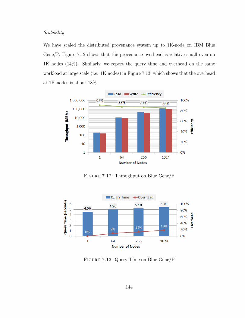
Scalability

We have scaled the distributed provenance system up to 1K-node on IBM Blue

Gene/P. Figure 7.12 shows that the provenance overhead is relative small even on

1K nodes (14%). Similarly, we report the query time and overhead on the same

workload at large scale (i.e. 1K nodes) in Figure 7.13, which shows that the overhead

at 1K-nodes is about 18%.

Figure 7.12: Throughput on Blue Gene/P

Figure 7.13: Query Time on Blue Gene/P

144

7.5 Summary

This chapter explores the feasibility of a general metadata storage and management

layer for parallel file systems, in which metadata includes both file operations and

provenance metadata. Two systems are investigated (1) FusionFS, which implements

a distributed file metadata management based on distributed hash tables, and (2)

SPADE, which uses a graph database to store audited provenance data and provides

distributed module for querying provenance. Our results on a 32-node cluster show

that FusionFS+SPADE is a promising prototype with negligible provenance overhead

and has promise to scale to petascale and beyond. Furthermore, FusionFS with its

own storage layer for provenance capture is able to scale up to 1K nodes on Blue

Gene/P supercomputer.

145

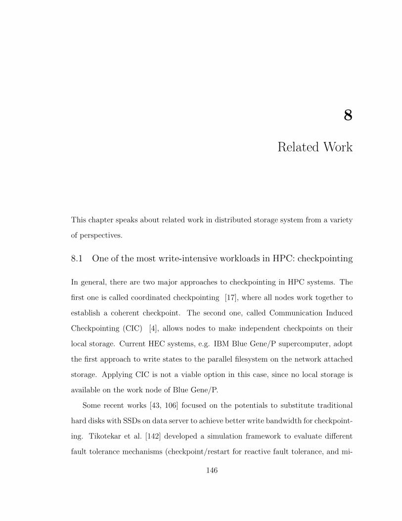
8

Related Work

This chapter speaks about related work in distributed storage system from a variety

of perspectives.

8.1 One of the most write-intensive workloads in HPC: checkpointing

In general, there are two major approaches to checkpointing in HPC systems. The

first one is called coordinated checkpointing [17], where all nodes work together to

establish a coherent checkpoint. The second one, called Communication Induced

Checkpointing (CIC) [4], allows nodes to make independent checkpoints on their

local storage. Current HEC systems, e.g. IBM Blue Gene/P supercomputer, adopt

the first approach to write states to the parallel filesystem on the network attached

storage. Applying CIC is not a viable option in this case, since no local storage is

available on the work node of Blue Gene/P.

Some recent works [43, 106] focused on the potentials to substitute traditional

hard disks with SSDs on data server to achieve better write bandwidth for checkpoint-

ing. Tikotekar et al. [142] developed a simulation framework to evaluate different

fault tolerance mechanisms (checkpoint/restart for reactive fault tolerance, and mi-

146

gration for pro-active fault tolerance). The framework uses system failure logs for

the simulation with a default behavior based on logs taken from the ASC White at

LLNL. A non-blocking checkpointing mode is proposed in [117] to support optimal

parallel discrete event simulation. This model allows real concurrency in the execu-

tion of state saving and other simulation specific operations (e.g. event list update,

event execution), with the aim at removing the cost of recording state information

from the parallel application. An incremental checkpointing/restart model is built

in [100], which is applied to the HPC environment. The model aims at reducing

full checkpointing overhead by performing a set of incremental updates between two

consecutive full checkpoints. Some recent research was focused on XOR-based meth-

ods, for example, [146] proposed reliable and fast in-memory checkpointing for MPI

programs and [23] presented a distributed checkpointing manner using XOR opera-

tions. None of these related works explored exascale systems, and none addressed the

checkpointing challenges through a different storage architecture (e.g. distributed file

systems).

8.2 Conventional parallel and distributed file systems

There have been many shared and parallel file systems, such as the Network File

System (NFS [33]), General Purpose File System (GPFS [129]), Parallel Virtual

File System (PVFS [20]), Lustre[130], and Panasas[99]. These systems assume that

storage nodes are significantly fewer than the compute nodes, and compute resources

are agnostic of the data locality on the underlying storage system, which results in

an unbalanced architecture for data-intensive workloads.

A variety of distributed file systems have been developed such as Google File

System (GFS [44]), Hadoop File System (HDFS [134]), Ceph [150], and Sector [49].

However, many of these file systems are tightly coupled with execution frameworks

(e.g. MapReduce [27]), which means that scientific applications not using these

147

frameworks must be modified to use these non-POSIX file systems. For those that

offer a POSIX interface, they are not designed for metadata-intensive operations

at extreme scales. The majority of these systems do not expose the data locality

information for general computational frameworks (e.g. batch schedulers, workflow

systems) to harness the data locality through data-aware scheduling. In short, these

distributed file systems are not designed specifically for HPC and scientific computing

workloads, and the scales that HPC are anticipating in the coming years.

The idea of distributed metadata can be traced back to xFS [7], even though

a central manager is in need to locate a particular file. Recently, FDS [103] was

proposed as a blob store on data centers. It maintains a lightweight metadata server

and offloads the metadata to available nodes in a distributed manner. In contrast,

FusionFS metadata is completely distributed without any single component involved.

GIGA+ [109] addressed challenges from big directories where millions to billions of

small files are created in a single directory. The metadata throughput of GIGA+

significantly outperforms the traditional distributed directory implementations at up

to 32-node scales. However, it is not clear if this design would suffice for extreme

scales, e.g. 1K nodes and beyond.

Co-location of compute and storage resources has attracted a lot of research

interests. For instance, Salus [148] proposes to co-locate the storage to data nodes in

data centers. Other examples include Rhea [45], which prevents removing the data

used by the computation, and Nectar [51], which automatically manages data and

computation in data centers. While these systems apply a general rule to deal with

data I/O, FusionFS is optimized for write-intensive workloads that are particularly

important for HPC systems.

148

8.3 Filesystem caching

To the best of our knowledge, HyCache is the first user-level POSIX-compliant hybrid

caching for distributed file systems. Some of our previous work [119, 122] proposed

data caching to accelerate applications by modifying the applications and/or their

workflow, rather than the at the filesystem level. Other existing work requires mod-

ifying OS kernel, or lacks of a systematic caching mechanism for manipulating files

across multiple storage devices, or does not support the POSIX interface. Any of

the these concerns would limit the system’s applicability to end users. We will give

a brief review of previous studies on hybrid storage systems.

Some recent work reported the performance comparison between SSD and HDD

in more perspectives ([72, 136]). Hystor [22] aims to optimize of the hybrid storage of

SSDs and HDDs. However it requires to modify the kernel which might cause some

issues. A more general multi-tiering scheme was proposed in [50] which helps decide

the needed numbers of SSD/HDDs and manage the data shift between SSDs and

HDDs by adding a ‘pseudo device driver’, again, in the kernel. iTransformer [164]

considers the SSD as a traditional transient cache in which case data needs to be

written to the spinning hard disk at some point once the data is modified in the SSD.

iBridge [165] leverages SSD to serve request fragments and bridge the performance

gap between serving fragments and serving large sub-requests. HPDA [86] offers a

mechanism to plug SSDs into RAID in order to improve the reliability of the disk

array. SSD was also proposed to be integrated to the RAM level which makes SSD

as the primary holder of virtual memory [9]. NVMalloc [145] provides a library to

explicitly allow users to allocate virtual memory on SSD. Also for extending virtual

memory with Storage Class Memory (SCM), SCMFS [153] concentrates more on the

management of a single SCM device. FAST [64] proposed a caching system to pre-

fetch data in order to quicken the application launch. In [158] SSD is considered as

149

a read-only buffer and migrate those random-writes to HDD.

A thorough review of classical caching algorithms on large scale data-intensive

applications is recently reported in [34]. HyCache+ is different from the classical

cooperative caching [113] in that HyCache+ assumes persistent underlying storage

and manipulates data at the file level. As an example of distributed caching for

distributed file systems, Blue Whale Cooperative Caching (BWCC) [132] is a read-

only caching system for cluster file systems. In contrast, HyCache+ is a POSIX-

compliant I/O storage middleware that transparently interacts with the underlying

parallel file systems. Even though the focus of this paper lies on the 2-layer hierarchy

of a local cache (e.g. SSD) and a remote parallel file system (e.g. GPFS [129]), the

approach presented in HyCache+ is applicable to multi-tier caching architecture as

well. Multi-level caching gains much research interest, especially in the emerging age

of cloud computing where the hierarchy of (distributed) storage is being redefined

with more layers. For example Hint-K [152] caching is proposed to keep track of the

last K steps across all the cache levels, which generalizes the conventional LRU-K

algorithm concerned only on the single level information.

There are extensive studies on leveraging data locality for effective caching. Block

Locality Caching (BLC) [90] captures the backup and always uses the latest local-

ity information to achieve better performance for data deduplication systems. The

File Access corRelation Mining and Evaluation Reference model (FARMER) [154]

optimizes the large scale file system by correlating access patterns and semantic at-

tributes. In contrast, HyCache+ achieves data locality with a unique mix of two

principles: (1) write is always local, and (2) read locality depends on the novel 2LS

(§4.2.2) mechanism which schedules jobs in a deterministic manner followed by a

local heuristic replacement policy.

While HyCache+ presents a pure software solution for distributed cache, some

orthogonal work focuses on improving caching from the hardware perspective. In [76],

150

a hardware design is proposed with low overhead to support effective shared caches

in multicore processors. For shared last-level caches, COOP [163] is proposed to only

use one bit per cache line for re-reference prediction and optimize both locality and

utilization. The REDCAP project [47] aims to logically enlarge the disk cache by

using a small portion of main memory, so that the read time could be reduced. For

Solid-State Drive (SSD), a new algorithm called lazy adaptive replacement cache [57]

is proposed to improve the cache hit and prolong the SSD lifetime.

Power-efficient caching has drawn a lot of research interests. It is worth mention-

ing that HyCache+ aims to better meet the need of high I/O performance for HPC

systems, and power consumption is not the major consideration at this point. Nev-

ertheless, it should be noted that power consumption is indeed one of the toughest

challenges to be overcome in future systems. One of the earliest work [186] tried to

minimize the energy consumption by predicting the access mode and allowing cache

accesses to switch between the prediction and the access modes. Recently, a new

caching algorithm [160] was proposed to save up to 27% energy and reduce the mem-

ory temperature up to 5.450C with negligible performance degradation. EEVFS [85]

provides energy efficiency at the file system level with an energy-aware data layout

and the prediction on disk idleness.

While HyCache+ is architected for large scale HPC systems, caching has been

extensively studied in different subjects and fields. In cloud storage, Update-batched

Delayed Synchronization (UDS) [75] reduces the synchronization cost by buffering the

frequent and short updates from the client and synchronizing with the underlying

infrastructure in a batch fashion. For continuous data (e.g. online video), a new

algorithm called Least Waiting Probability (LWP) [157] is proposed to optimize

the newly defined metric called user waiting rate. In geoinformatics, the method

proposed in [71] considers both global and local temporal-spatial changes to achieve

high cache hit rate and short response time.

151

The job scheduler proposed in this work (§4.2.2) takes a greedy strategy to achieve

the optimal solution for the HyCache+ architecture. A more general, and more dif-

ficult, scheduling problem could be solved in a similar heuristic approach [116, 141].

For an even more general combinatorial optimization problem in a network, both

precise and bound-proved low-degree polynomial approximation algorithms were re-

ported in [16, 15]. Some incremental approaches [178, 79, 177] were proposed to

efficiently retain the strong connectivity of a network and solve the satisfiability

problem with constraints.

In future, we plan to better predict the I/O behavior by employing some machine

learning techniques such as incremental algorithms, as well as more advanced data-

aware scheduling mechanisms [178, 79, 177] such as [147].

8.4 Filesystem compression

While the storage system could be better deigned to handle more data, an orthogonal

approach is to address the I/O bottleneck by squeezing the data with compression

techniques. One example where data compression gets particularly popular is check-

pointing, an extremely expensive I/O operation in HPC systems. In [35], it showed

that data compression had the potential to significantly reduce the checkpointing file

sizes. If multiple applications run concurrently, a data-aware compression scheme [60]

was proposed to improve the overall checkpointing efficiency. Recent study [12] shows

that combining failure detection and proactive checkpointing could improve 30% ef-

ficiency compared to classical periodical checkpointing. Thus data compression has

the potential to be combined with failure detection and proactive checkpointing to

further improve the system efficiency. As another example, data compression was

also used in reducing the MPI trace size, as shown in [104]. A small MPI trace

enables an efficient replay and analysis of the communication patterns in large-scale

machines.

152

It should be noted that a compression method does not necessarily need to restore

the absolutely original data. In general, compression algorithms could be categorized

into to two groups: lossy algorithms and lossless algorithms. A lossy algorithm

might lose some (normally a small) percentage of accuracy, while a lossless one

has to ensure the 100% accuracy. In scientific computing, studies [70, 69] show

that lossy compression could be acceptable, or even quite effective, under certain

circumstances. In fact, lossy compression is also popular in other fields, e.g. the

most widely compatible lossy audio and video format MPEG-1 [93]. This paper

presents virtual chunks mostly by going through a delta-compression example based

on XOR, which is a lossless compression. It does not imply that virtual chunks

cannot be used in a lossy compression. Virtual chunk is not a specific compression

algorithm, but a system mechanism that is applicable to any splittable compression,

not matter if it is lossy or lossless.

Some frameworks are proposed as middleware to allow applications call high-

level I/O libraries for data compression and decompression, e.g. [11, 128, 62]. None

of these techniques take consideration of the overhead involved in decompression

by assuming the chunk allocated to each node would be requested as an entirety.

In contrast, virtual chunks provide a mechanism to apply flexible compression and

decompression.

There is previous work to study the file system support for data compression. In-

tegrating compression to log-structured file systems was proposed decades ago [13],

which suggested a hardware compression chip to accelerate the compressing and de-

compressing. Later, XDFS [83] described the systematic design and implementation

for supporting data compression in file systems with BerkeleyDB [105]. MRAMFS [32]

was a prototype file system to support data compression to leverage the limited space

of non-volatile RAM. In contrast, virtual trunks represent a general technique appli-

cable to existing algorithms and systems.

153

Data deduplication is a general inter-chunk compression technique that only

stores a single copy of the duplicate chunks (or blocks). For example, LBFS [98]

was a networked file system that exploited the similarities between files (or versions

of files) so that chunks of files could be retrieved in the client’s cache rather than

transferring from the server. CZIP [107] was a compression scheme on content-

based naming, that eliminated redundant chunks and compressed the remaining (i.e.

unique) chunks by applying existing compression algorithms. Recently, the metadata

for the deduplication (i.e. file recipe) was also slated for compression to further save

the storage space [89]. While deduplication focuses on inter-chunk compressing,

virtual chunk focuses on the I/O improvement within the chunk.

Index has been introduced to data compression to improve the compressing and

query speed e.g. [68, 46]. The advantage of indexing is highly dependent on the

chunk size: large chunks are preferred to achieve high compression ratios in order to

amortize the indexing overhead. Large chunks, however, would cause potential de-

compression overhead as explained earlier in this paper. Virtual chunk overcomes the

large-chunk issue by logically splitting the large chunks with fine-grained partitions

while still keeping the physical coherence.

8.5 Filesystem provenance

As distributed systems become more ubiquitous and complex, there is a growing

emphasis on the need for tracking provenance metadata along with file system meta-

data. A thorough review is presented in [94]. Many Grid systems like Chimera [37]

and the Provenance-Aware Service Oriented Architecture (PASOA) [115] provide

provenance tracking mechanisms for various applications. However these systems

are very domain specific and do not capture provenance at the filesystem level. The

Distributed Provenance Aware Storage System (DPASS) tracks the provenance of

files in a distributed file system by intercepting filesystem operations and sending

154

this information via a netlink socket to user level daemon that collects provenance

in a database server [108]. The provenance is however, collected in a centralized

fashion, which is a poor design choice for distributed file systems meant for extreme

scales. Similarly in efficient retrieval of files, provenance is collected centrally [96].

PASS describes global naming, indexing, and querying in the context of sensor

data [97]. PA-NFS [95] enhances NFS to record provenance in local area networks

but does not consider distributed naming explicitly. SPADE [42] addresses the issue

by using storage identifiers for provenance vertices that are unique to a host and

requiring distributed provenance queries to disambiguate vertices by referring to

them by the host on which the vertex was generated as well as the identifier local to

that host.

Several storage systems have been considered for storing provenance. ExSPAN [185]

extends traditional relational models for storing and querying provenance metadata.

SPADE supports both graph and relational database storage and querying. PASS

has explored the use of clouds [97]. Provbase uses Hbase to store and query scien-

tific workflow provenance [1]. Further compressing provenance [185], indexing [84]

and optimization techniques [55] have also been considered. However, none of these

systems have been tested for exascale architectures. To give adequate merit to the

previous designs we have integrated FusionFS with SPADE as well as considered

FusionFS’ internal storage system for storing audited provenance.

155

9

Conclusion and Future Work

In summary, this work identifies the storage bottleneck of extreme-scale HPC systems

and proposes a new architecture to overcome it. We build a system prototype—the

Fusion distributed file system (FusionFS)—to verify the effectiveness of this new

architecture, and explore unique features (for example, caching, compression, relia-

bility, and provenance) that are unsupported in conventional storage systems. Our

extensive evaluations demonstrate that the proposed architecture, along with the

FusionFS implementation, would ameliorate the storage bottleneck of the future ex-

ascale HPC systems.

With a working distributed filesystem FusionFS on hand, there will be many

directions for our future work. Among them, we plan to extend our current work

into the following three directions.

9.1 FusionFS Simulation at Exascale

This project will concentrate on FusionFS’s own performance and scalability at ex-

treme scales. We plan to develop a simulator of FusionFS called FusionSim, and

validate it by real FusionFS traces at medium scale e.g. O(10K) nodes. We will then

156

scale FusionSim to exascale (i.e., O(1M)) nodes, and report its performance. If time

permits, we will also simulate real applications on FusionFS at exascale.

With this significant extension on exascale simulation, the FusionFS work will be

submitted to IEEE Transactions on Parallel and Distributed Systems.

9.2 Dynamic Virtual Chunks on Compressible Filesystems

If the access pattern does not follow the uniform distribution, and this information is

exposed to users, then it makes sense to specify more references (i.e. finer granularity

of virtual chunks) for the subset that is more frequently accessed. This is because

more references make random accesses more efficiently with a shorter distance (and

less computation) from the closest reference, in general. The assumption of equidis-

tant reference, thus, does not hold any more as in our previous discussion on virtual

chunks.

We will consider a more general scenario where the virtual chunks are not nec-

essarily equidistant (i.e. dynamic virtual chunks), but can be adjusted dynamically.

A set of new procedures are devised with a user-specified updating strategy, which

could be on the basis of affected range of data and a linear transform of the static

virtual chunks.

With this significant extension on dynamic reference allocation, the virtual chunk

work will be submitted to IEEE Transactions on Service Computing.

9.3 Locality-Aware Data Management on FusionFS

As an analogy to the Hadoop software stack where the data are manipulated by

MapReduce on a customized filesystem HDFS, we plan to integrate a workflow sys-

tem (e.g. Swift [183]) into FusionFS so that applications specified in a workflow

system could automatically take advantage of the data locality exposed by the data

157

management and its underlying filesystem. We are working closely with Argonne Na-

tional Laboratory, and expecting to submit the preliminary results of Swift-FusionFS

integration to the ACM HPDC’15 conference in January 2015.

9.4 Timeline

• Soon, revise journal papers [175, 74] currently under review.

• 11/2014, submit dynamic virtual chunks to IEEE Transactions on Service Com-

puting.

• 12/2014, submit FusionFS exascale simulation to IEEE Transactions on Par-

allel and Distributed Systems.

• 01/2015, submit Swift-FusionFS integration to ACM HPDC’15 conference.

• 04/2015, submit extended Swift-FusionFS work to IEEE Transactions on Com-

puters.

• 12/2015, plan to graduate.

158

Bibliography

[1] J. Abraham, P. Brazier, A. Chebotko, J. Navarro, and A. Piazza. Distributedstorage and querying techniques for a semantic web of scientific workflow prove-nance. In Services Computing (SCC), 2010 IEEE International Conference on,pages 178–185. IEEE, 2010.

[2] S. Albers, N. Garg, and S. Leonardi. Minimizing stall time in single and paralleldisk systems. In Proceedings of the thirtieth annual ACM symposium on Theoryof computing, 1998.

[3] N. Ali, P. Carns, K. Iskra, D. Kimpe, S. Lang, R. Latham, R. Ross, L. Ward,and P. Sadayappan. Scalable i/o forwarding framework for high-performancecomputing systems. In Cluster Computing and Workshops, 2009. CLUS-TER’09. IEEE International Conference on, 2009.

[4] L. Alvisi, E. Elnozahy, S. Rao, S. Husain, and A. de Mel. An analysis ofcommunication induced checkpointing. In Fault-Tolerant Computing, 1999.Digest of Papers. Twenty-Ninth Annual International Symposium on, 1999.

[5] Amazon EC2. http://aws.amazon.com/ec2, 2014.

[6] C. Ambuhl and B. Weber. Parallel prefetching and caching is hard. In STACS,2004.

[7] T. E. Anderson, M. D. Dahlin, J. M. Neefe, D. A. Patterson, D. S. Roselli,and R. Y. Wang. Serverless network file systems. In Proceedings of ACMsymposium on Operating systems principles, 1995.

[8] Apache Hadoop. http://hadoop.apache.org/, Accessed September 5, 2014.

[9] A. Badam and V. S. Pai. SSDAlloc: hybrid SSD/RAM memory managementmade easy. In Proceedings of the 8th USENIX conference on Networked systemsdesign and implementation, 2011.

[10] R. Bellman. Dynamic programming treatment of the travelling salesman prob-lem. J. ACM, 9(1), Jan. 1962.

159

[11] T. Bicer, J. Yin, D. Chiu, G. Agrawal, and K. Schuchardt. Integrating onlinecompression to accelerate large-scale data analytics applications. In Proceedingsof the 2013 IEEE 27th International Symposium on Parallel and DistributedProcessing (IPDPS), 2013.

[12] M. S. Bouguerra, A. Gainaru, L. B. Gomez, F. Cappello, S. Matsuoka, andN. Maruyam. Improving the computing efficiency of hpc systems using a com-bination of proactive and preventive checkpointing. In Parallel DistributedProcessing, IEEE International Symposium on, 2013.

[13] M. Burrows, C. Jerian, B. Lampson, and T. Mann. On-line data compressionin a log-structured file system. In Proceedings of the Fifth International Con-ference on Architectural Support for Programming Languages and OperatingSystems (ASPLOS), 1992.

[14] bzip2. http://www.bzip2.org, Accessed September 5, 2014.

[15] G. Calinescu, S. Kapoor, K. Qiao, and J. Shin. Stochastic strategic routing re-duces attack effects. In Global Telecommunications Conference (GLOBECOM2011), 2011 IEEE, 2011.

[16] G. Calinescu and K. Qiao. Asymmetric topology control: Exact solutions andfast approximations. In IEEE International Conference on Computer Commu-nications (INFOCOM ’12), 2012.

[17] G. Cao and M. Singhal. On coordinated checkpointing in distributed systems.Parallel and Distributed Systems, IEEE Transactions on, 9(12), dec 1998.

[18] P. Cao, E. W. Felten, A. R. Karlin, and K. Li. A study of integrated prefetchingand caching strategies. SIGMETRICS Perform. Eval. Rev., 23(1), May 1995.

[19] P. Carns, S. Lang, R. Ross, M. Vilayannur, J. Kunkel, and T. Ludwig. Small-fileaccess in parallel file systems. In Proceedings of IEEE International Symposiumon Parallel and Distributed Processing, 2009.

[20] P. H. Carns, W. B. Ligon, R. B. Ross, and R. Thakur. PVFS: A parallel filesystem for linux clusters. In Proceedings of the 4th Annual Linux Showcaseand Conference, 2000.

[21] S. Che, M. Boyer, J. Meng, D. Tarjan, J. W. Sheaffer, and K. Skadron. Aperformance study of general-purpose applications on graphics processors usingcuda. J. Parallel Distrib. Comput., 68(10):1370–1380, Oct. 2008.

[22] F. Chen, D. A. Koufaty, and X. Zhang. Hystor: Making the best use ofsolid state drives in high performance storage systems. In Proceedings of theInternational Conference on Supercomputing, 2011.

160

[23] G.-M. Chiu and J.-F. Chiu. A new diskless checkpointing approach for multipleprocessor failures. IEEE Trans. Dependable Secur. Comput., 8(4), July 2011.

[24] E. Cohen and M. Strauss. Maintaining time-decaying stream aggregates. InProceedings of the Twenty-second ACM SIGMOD-SIGACT-SIGART Sympo-sium on Principles of Database Systems, 2003.

[25] M. L. Curry, A. Skjellum, H. Lee Ward, and R. Brightwell. Gibraltar: Areed-solomon coding library for storage applications on programmable graphicsprocessors. Concurr. Comput. : Pract. Exper., 23(18):2477–2495, Dec. 2011.

[26] J. Daly. A model for predicting the optimum checkpoint interval for restartdumps. In Proceedings of the 2003 International Conference on ComputationalScience, 2003.

[27] J. Dean and S. Ghemawat. MapReduce: Simplified data processing on largeclusters. In Proceedings of USENIX Symposium on Opearting Systems Design& Implementation, 2004.

[28] G. DeCandia, D. Hastorun, M. Jampani, G. Kakulapati, A. Lakshman,A. Pilchin, S. Sivasubramanian, P. Vosshall, and W. Vogels. Dynamo: Ama-zon’s highly available key-value store. SIGOPS Oper. Syst. Rev., 41(6):205–220,Oct. 2007.

[29] DEEP-ER. http://www.hpc.cineca.it/projects/deep-er, Accessed September5, 2014.

[30] X. Dong, Y. Xie, N. Muralimanohar, and N. P. Jouppi. Hybrid checkpointingusing emerging nonvolatile memories for future exascale systems. ACM Trans.Archit. Code Optim., 8(2), June 2011.

[31] M. Dorier, G. Antoniu, F. Cappello, M. Snir, and L. Orf. Damaris: How toefficiently leverage multicore parallelism to achieve scalable, jitter-free I/O. InProceedings of IEEE International Conference on Cluster Computing, 2012.

[32] N. K. Edel, D. Tuteja, E. L. Miller, and S. A. Brandt. Mramfs: A compressingfile system for non-volatile ram. In Proceedings of the The IEEE ComputerSociety’s 12th Annual International Symposium on Modeling, Analysis, andSimulation of Computer and Telecommunications Systems (MASCOTS), 2004.

[33] M. Eisler, R. Labiaga, and H. Stern. Managing NFS and NIS, 2nd ed. O’Reilly& Associates, Inc., 2001.

[34] R. Fares, B. Romoser, Z. Zong, M. Nijim, and X. Qin. Performance evaluationof traditional caching policies on a large system with petabytes of data. InNetworking, Architecture and Storage (NAS), 2012 IEEE 7th InternationalConference on, 2012.

161

[35] K. B. Ferreira, R. Riesen, D. Arnold, D. Ibtesham, and R. Brightwell. Theviability of using compression to decrease message log sizes. In Proceedings ofInternational Conference on Parallel Processing Workshops, 2013.

[36] B. Fitzpatrick. Distributed caching with memcached. Linux J., 2004(124),Aug. 2004.

[37] I. T. Foster, J.-S. Vckler, M. Wilde, and Y. Zhao. The virtual data grid: A newmodel and architecture for data-intensive collaboration. In CIDR’03, 2003.

[38] P. Freeman, D. Crawford, S. Kim, and J. Munoz. Cyberinfrastructure forscience and engineering: Promises and challenges. Proceedings of the IEEE,93(3), 2005.

[39] P. A. Freeman, D. L. Crawford, S. Kim, and J. L. Munoz. Cyberinfrastructurefor science and engineering: Promises and challenges. Proceedings of the IEEE,93(3):682–691, 2005.

[40] FUSE. http://fuse.sourceforge.net, Accessed September 5, 2014.

[41] GCRM. http://kiwi.atmos.colostate.edu/gcrm/, Accessed September 5, 2014.

[42] A. Gehani and D. Tariq. SPADE: Support for Provenance Auditing in Dis-tributed Environments. In Proceedings of the 13th International MiddlewareConference, 2012.

[43] S. Gerhold, N. Kaemmer, A. Weggerle, C. Himpel, and P. Schulthess. Page-server: High-performance ssd-based checkpointing of transactional distributedmemory. In Computer Engineering and Applications (ICCEA), 2010 SecondInternational Conference on, volume 1, march 2010.

[44] S. Ghemawat, H. Gobioff, and S.-T. Leung. The Google file system. In Pro-ceedings of the Nineteenth ACM Symposium on Operating Systems Principles,2003.

[45] C. Gkantsidis, D. Vytiniotis, O. Hodson, D. Narayanan, F. Dinu, and A. Row-stron. Rhea: automatic filtering for unstructured cloud storage. In Proceedingsof the 10th USENIX conference on Networked Systems Design and Implemen-tation, 2013.

[46] Z. Gong, S. Lakshminarasimhan, J. Jenkins, H. Kolla, S. Ethier, J. Chen,R. Ross, S. Klasky, and N. F. Samatova. Multi-level layout optimization forefficient spatio-temporal queries on isabela-compressed data. In Proceedings ofthe 2012 IEEE 26th International Parallel and Distributed Processing Sympo-sium (IPDPS), 2012.

162

[47] P. Gonzalez-Ferez, J. Piernas, and T. Cortes. The ram enhanced disk cacheproject (redcap). In Proceedings of the 24th IEEE Conference on Mass StorageSystems and Technologies, 2007.

[48] Y. Gu and R. L. Grossman. Supporting configurable congestion control indata transport services. In Proceedings of the 2005 ACM/IEEE Conference onSupercomputing, 2005.

[49] Y. Gu, R. L. Grossman, A. Szalay, and A. Thakar. Distributing the Sloan Dig-ital Sky Survey using UDT and Sector. In Proceedings of IEEE InternationalConference on e-Science and Grid Computing, 2006.

[50] J. Guerra, H. Pucha, J. Glider, W. Belluomini, and R. Rangaswami. Costeffective storage using extent based dynamic tiering. In Proceedings of the 9thUSENIX conference on File and stroage technologies, 2011.

[51] P. K. Gunda, L. Ravindranath, C. A. Thekkath, Y. Yu, and L. Zhuang. Nectar:automatic management of data and computation in datacenters. In Proceedingsof the 9th USENIX conference on Operating systems design and implementation(OSDI), 2010.

[52] Gzip. http://www.gnu.org/software/gzip/gzip.html, Accessed September 5,2014.

[53] J. L. Hafner, V. Deenadhayalan, K. K. Rao, and J. A. Tomlin. Matrix methodsfor lost data reconstruction in erasure codes. 2005.

[54] HDF5. http://www.hdfgroup.org/hdf5/doc/index.html, Accessed September5, 2014.

[55] T. Heinis and G. Alonso. Efficient lineage tracking for scientific workflows. InProceedings of the 2008 ACM SIGMOD international conference on Manage-ment of data, pages 1007–1018, 2008.

[56] T. Hey, S. Tansley, and K. Tolle, editors. The Fourth Paradigm: Data-IntensiveScientific Discovery. Microsoft Research, 2009.

[57] S. Huang, Q. Wei, J. Chen, C. Chen, and D. Feng. Improving flash-based diskcache with lazy adaptive replacement. In Mass Storage Systems and Technolo-gies (MSST), 2013 IEEE 29th Symposium on, 2013.

[58] Intrepid. https://www.alcf.anl.gov/user-guides/intrepid-challenger-surveyor,Accessed September 5, 2014.

[59] IOZone. http://www.iozone.org, 2014.

163

[60] T. Z. Islam, K. Mohror, S. Bagchi, A. Moody, B. R. de Supinski, and R. Eigen-mann. McrEngine: A scalable checkpointing system using data-aware aggrega-tion and compression. In Proceedings of the International Conference on HighPerformance Computing, Networking, Storage and Analysis (SC), 2012.

[61] James N. England. A system for interactive modeling of physical curved surfaceobjects. pages 336–340, 1978.

[62] J. Jenkins, E. R. Schendel, S. Lakshminarasimhan, D. A. Boyuka, II, T. Rogers,S. Ethier, R. Ross, S. Klasky, and N. F. Samatova. Byte-precision level of detailprocessing for variable precision analytics. In Proceedings of the InternationalConference on High Performance Computing, Networking, Storage and Anal-ysis (SC), 2012.

[63] X. Jiang, M. Alghamdi, J. Zhang, M. Assaf, X. Ruan, T. Muzaffar, and X. Qin.Thermal modeling and analysis of storage systems. In Performance Comput-ing and Communications Conference (IPCCC), 2012 IEEE 31st International,2012.

[64] Y. Joo, J. Ryu, S. Park, and K. G. Shin. FAST: Quick application launch onsolid-state drives. In Proceedings of the 9th USENIX Conference on File andStroage Technologies, 2011.

[65] J. Katcher. Postmark: A new file system benchmark. In Network Appliance,Inc., volume 3022, 1997.

[66] O. Khan, R. Burns, J. Plank, W. Pierce, and C. Huang. Rethinking erasurecodes for cloud file systems: Minimizing I/O for recovery and degraded reads.2012.

[67] Kodiak. https://www.nmc-probe.org/wiki/machines:kodiak, AccessedSeptember 5, 2014.

[68] S. Lakshminarasimhan, D. A. Boyuka, S. V. Pendse, X. Zou, J. Jenkins,V. Vishwanath, M. E. Papka, and N. F. Samatova. Scalable in situ scien-tific data encoding for analytical query processing. In Proceedings of the 22ndInternational Symposium on High-performance Parallel and Distributed Com-puting (HPDC), 2013.

[69] S. Lakshminarasimhan, J. Jenkins, I. Arkatkar, Z. Gong, H. Kolla, S.-H. Ku,S. Ethier, J. Chen, C. S. Chang, S. Klasky, R. Latham, R. Ross, and N. F.Samatova. ISABELA-QA: Query-driven analytics with ISABELA-compressedextreme-scale scientific data. In Proceedings of 2011 International Conferencefor High Performance Computing, Networking, Storage and Analysis (SC’11),2011.

164

[70] D. Laney, S. Langer, C. Weber, P. Lindstrom, and A. Wegener. Assessing theeffects of data compression in simulations using physically motivated metrics.In Proceedings of the International Conference on High Performance Comput-ing, Networking, Storage and Analysis, 2013.

[71] R. Li, R. Guo, Z. Xu, and W. Feng. A prefetching model based on accesspopularity for geospatial data in a cluster-based caching system. Int. J. Geogr.Inf. Sci., 26(10), Oct. 2012.

[72] S. Li and H. Huang. Black-box performance modeling for solid-state drives. InModeling, Analysis Simulation of Computer and Telecommunication Systems(MASCOTS), 2010 IEEE International Symposium on, 2010.

[73] T. Li, X. Zhou, K. Brandstatter, D. Zhao, K. Wang, A. Rajendran, Z. Zhang,and I. Raicu. ZHT: A light-weight reliable persistent dynamic scalable zero-hop distributed hash table. In Proceedings of IEEE International Symposiumon Parallel and Distributed Processing, 2013.

[74] T. Li, X. Zhou, K. Brandstatter, D. Zhao, K. Wang, Z. Zhang, and I. Raicu.A convergence of nosql distributed key/value storage in cloud computing andsupercomputing. IEEE Transaction on Service Computing, Special Issue onCloud Computing(under review), 2014.

[75] Z. Li, C. Wilson, Z. Jiang, Y. Liu, B. Zhao, C. Jin, Z.-L. Zhang, and Y. Dai.Efficient batched synchronization in dropbox-like cloud storage services. InProceedings of the 14th International Middleware Conference, 2013.

[76] J. Lin, Q. Lu, X. Ding, Z. Zhang, X. Zhang, and P. Sadayappan. Enabling soft-ware management for multicore caches with a lightweight hardware support.In Proceedings of the 2009 ACM/IEEE conference on Supercomputing, 2009.

[77] N. Liu, J. Cope, P. H. Carns, C. D. Carothers, R. B. Ross, G. Grider, A. Crume,and C. Maltzahn. On the role of burst buffers in leadership-class storage sys-tems. In Proceedings of IEEE Symposium on Mass Storage Systems and Tech-nologies, 2012.

[78] W. Liu, B. Schmidt, G. Voss, A. Schroder, and W. Muller-Wittig. Bio-sequencedatabase scanning on a gpu. In Proceedings of the 20th International Confer-ence on Parallel and Distributed Processing, 2006.

[79] R. Lohfert, J. Lu, and D. Zhao. Solving sql constraints by incremental transla-tion to sat. In International Conference on Industrial, Engineering and OtherApplications of Applied Intelligent Systems, 2008.

[80] LZO. http://www.oberhumer.com/opensource/lzo, Accessed September 5,2014.

165

[81] K.-L. Ma. In situ visualization at extreme scale: Challenges and opportunities.Computer Graphics and Applications, IEEE, 29(6), 2009.

[82] K.-L. Ma, C. Wang, H. Yu, and A. Tikhonova. In-situ processing and visu-alization for ultrascale simulations. In Journal of Physics: Conference Series,volume 78, 2007.

[83] J. P. MacDonald. File system support for delta compression. Technical report,University of California, Berkley, 2000.

[84] T. Malik, A. Gehani, D. Tariq, and F. Zaffar. Sketching distributed dataprovenance. In Data Provenance and Data Management in eScience, pages85–107. 2013.

[85] A. Manzanares, X. Ruan, S. Yin, J. Xie, Z. Ding, Y. Tian, J. Majors, andX. Qin. Energy efficient prefetching with buffer disks for cluster file systems. InProceedings of the 2010 39th International Conference on Parallel Processing,2010.

[86] B. Mao, H. Jiang, D. Feng, S. Wu, J. Chen, L. Zeng, and L. Tian. HPDA:A hybrid parity-based disk array for enhanced performance and reliability. InParallel Distributed Processing (IPDPS), 2010 IEEE International Symposiumon, 2010.

[87] D. R. Mathog. Parallel BLAST on split databases. Bioinformatics, 19(4):1865– 1866, 2003.

[88] A. J. McAuley. Reliable broadband communication using a burst erasure cor-recting code. pages 297–306, 1990.

[89] D. Meister, A. Brinkmann, and T. Suß. File recipe compression in data dedu-plication systems. In Proceedings of the 11th USENIX Conference on File andStorage Technologies (FAST), 2013.

[90] D. Meister, J. Kaiser, and A. Brinkmann. Block locality caching for datadeduplication. In Proceedings of the 6th International Systems and StorageConference, 2013.

[91] Microsoft Azure. https://azure.microsoft.com, 2014.

[92] Mira. https://www.alcf.anl.gov/user-guides/mira-cetus-vesta, AccessedSeptember 5, 2014.

[93] MPEG-1. http://en.wikipedia.org/wiki/mpeg-1, Accessed September 5, 2014.

[94] K.-K. Muniswamy-Reddy. Foundations for provenance-aware systems. 2010.

166

[95] K.-K. Muniswamy-Reddy, U. Braun, D. A. Holland, P. Macko, D. Maclean,D. Margo, M. Seltzer, and R. Smogor. Layering in provenance systems. InProceedings of the 2009 USENIX Annual Technical Conference, 2009.

[96] K.-K. Muniswamy-Reddy, D. A. Holland, U. Braun, and M. Seltzer.Provenance-aware storage systems. In Proceedings of the annual conferenceon USENIX ’06 Annual Technical Conference, 2006.

[97] K.-K. Muniswamy-Reddy, P. Macko, and M. Seltzer. Making a cloudprovenance-aware. In 1st Workshop on the Theory and Practice of Provenance,2009.

[98] A. Muthitacharoen, B. Chen, and D. Mazieres. A low-bandwidth networkfile system. In Proceedings of the Eighteenth ACM Symposium on OperatingSystems Principles (SOSP), 2001.

[99] D. Nagle, D. Serenyi, and A. Matthews. The Panasas activescale storage clus-ter: Delivering scalable high bandwidth storage. In Proceedings of ACM/IEEEConference on Supercomputing, 2004.

[100] N. Naksinehaboon, Y. Liu, C. B. Leangsuksun, R. Nassar, M. Paun, and S. L.Scott. Reliability-aware approach: An incremental checkpoint/restart modelin hpc environments. In Proceedings of the 2008 Eighth IEEE InternationalSymposium on Cluster Computing and the Grid, 2008.

[101] NetCDF. http://www.unidata.ucar.edu/software/netcdf, Accessed September5, 2014.

[102] J. Nickolls, I. Buck, M. Garland, and K. Skadron. Scalable parallel program-ming with cuda. Queue, 6(2):40–53, Mar. 2008.

[103] E. B. Nightingale, J. Elson, J. Fan, O. Hofmann, J. Howell, and Y. Suzue.Flat datacenter storage. In Proceedings of USENIX Symposium on OperatingSystems Design and Implementation, 2012.

[104] M. Noeth, J. Marathe, F. Mueller, M. Schulz, and B. de Supinski. Scalablecompression and replay of communication traces in massively parallel environ-ments. In Proceedings of the 2006 ACM/IEEE Conference on Supercomputing(SC), 2006.

[105] M. A. Olson, K. Bostic, and M. Seltzer. Berkeley db. In Proceedings of theAnnual Conference on USENIX Annual Technical Conference, 1999.

[106] X. Ouyang, S. Marcarelli, and D. K. Panda. Enhancing Checkpoint Perfor-mance with Staging IO and SSD. In Proceedings of the 2010 InternationalWorkshop on Storage Network Architecture and Parallel I/Os, 2010.

167

[107] K. Park, S. Ihm, M. Bowman, and V. S. Pai. Supporting practical content-addressable caching with czip compression. In 2007 USENIX Annual TechnicalConference, 2007.

[108] A. Parker-Wood, D. D. E. Long, E. L. Miller, M. Seltzer, and D. Tunkelang.Making sense of file systems through provenance and rich metadata. TechnicalReport UCSC-SSRC-12-01, University of California, Santa Cruz, Mar. 2012.

[109] S. Patil and G. Gibson. Scale and concurrency of GIGA+: file system direc-tories with millions of files. In Proceedings of the 9th USENIX conference onFile and stroage technologies, 2011.

[110] J. S. Plank. Jerasure: A library in C/C++ facilitating erasure coding forstorage applications. Technical report, University of Tennessee, 2007.

[111] J. S. Plank, M. Blaum, and J. L. Hafner. SD Codes: Erasure codes designed forhow storage systems really fail. In Proceedings of the 11th USENIX conferenceon File and Storage Technologies, 2013.

[112] J. S. Plank, J. Luo, C. D. Schuman, L. Xu, and Z. Wilcox-O’Hearn. A perfor-mance evaluation and examination of open-source erasure coding libraries forstorage. In Proccedings of the 7th Conference on File and Storage Technologies,2009.

[113] S. Podlipnig and L. Boszormenyi. A survey of web cache replacement strategies.ACM Comput. Surv., 35(4), Dec. 2003.

[114] Protocol Buffers. http://code.google.com/p/protobuf/, Accessed September 5,2014.

[115] Provenance aware service oriented architecture. http://twiki.pasoa.ecs.soton.ac.uk/bin/view/pasoa/webhome, 2014.

[116] K. Qiao, F. Tao, L. Zhang, and Z. Li. A ga maintained by binary heap andtransitive reduction for addressing psp. In Intelligent Computing and IntegratedSystems (ICISS), 2010 International Conference on, Oct 2010.

[117] F. Quaglia and A. Santoro. Nonblocking checkpointing for optimistic parallelsimulation: Description and an implementation. IEEE Trans. Parallel Distrib.Syst., 14(6), June 2003.

[118] I. Raicu, I. T. Foster, and P. Beckman. Making a case for distributed filesystems at exascale. In Proceedings of the third international workshop onLarge-scale system and application performance, 2011.

168

[119] I. Raicu, I. T. Foster, Y. Zhao, P. Little, C. M. Moretti, A. Chaudhary, andD. Thain. The quest for scalable support of data-intensive workloads in dis-tributed systems. In Proceedings of ACM International Symposium on HighPerformance Distributed Computing, 2009.

[120] I. Raicu, Z. Zhang, M. Wilde, I. Foster, P. Beckman, K. Iskra, and B. Clifford.Toward loosely coupled programming on petascale systems. In Proceedings ofthe 2008 ACM/IEEE conference on Supercomputing, 2008.

[121] I. Raicu, Y. Zhao, C. Dumitrescu, I. Foster, and M. Wilde. Falkon: a fast andlight-weight task execution framework. In Proceedings of the 2007 ACM/IEEEconference on Supercomputing, 2007.

[122] I. Raicu, Y. Zhao, I. T. Foster, and A. Szalay. Accelerating large-scale dataexploration through data diffusion. In Proceedings of the 2008 internationalworkshop on Data-aware distributed computing, 2008.

[123] A. Rajgarhia and A. Gehani. Performance and extension of user space filesystems. In Proceedings of ACM Symposium on Applied Computing, 2010.

[124] I. Reed and G. Solomon. Polynomial codes over certain finite fields. Journalof the Society of Industrial and Applied Mathematics, (2), 06/1960.

[125] L. Rizzo. Effective erasure codes for reliable computer communication proto-cols. SIGCOMM Comput. Commun. Rev., (2):24–36, Apr.

[126] R. Rodrigues and B. Liskov. High availability in DHTs: erasure coding vs.replication. In Proceedings of the 4th international conference on Peer-to-PeerSystems, 2005.

[127] B. Romoser, Z. Zong, R. Fares, J. Wood, and R. Ge. Using intelligent prefetch-ing to reduce the energy consumption of a large-scale storage system. In Per-formance Computing and Communications Conference (IPCCC), 2013 IEEE32nd International, 2013.

[128] E. R. Schendel, S. V. Pendse, J. Jenkins, D. A. Boyuka, II, Z. Gong, S. Lakshmi-narasimhan, Q. Liu, H. Kolla, J. Chen, S. Klasky, R. Ross, and N. F. Samatova.Isobar hybrid compression-i/o interleaving for large-scale parallel i/o optimiza-tion. In Proceedings of International Symposium on High-Performance Paralleland Distributed Computing, 2012.

[129] F. Schmuck and R. Haskin. GPFS: A shared-disk file system for large comput-ing clusters. In Proceedings of the 1st USENIX Conference on File and StorageTechnologies (FAST), 2002.

[130] P. Schwan. Lustre: Building a file system for 1,000-node clusters. In Proceedingsof the linux symposium, 2003.

169

[131] SDSS Query. http://cas.sdss.org/astrodr6/en/help/docs/realquery.asp, Accessed September 5, 2014.

[132] L. Shi, Z. Liu, and L. Xu. Bwcc: A fs-cache based cooperative caching systemfor network storage system. In Proceedings of the 2012 IEEE InternationalConference on Cluster Computing, 2012.

[133] C. Shou, D. Zhao, T. Malik, and I. Raicu. Towards a provenance-aware dis-tributed filesystem. In 5th Workshop on the Theory and Practice of Provenance(TaPP), 2013.

[134] K. Shvachko, H. Kuang, S. Radia, and R. Chansler. The hadoop distributedfile system. In Proceedings of IEEE Symposium on Mass Storage Systems andTechnologies, 2010.

[135] Snappy. https://code.google.com/p/snappy/, Accessed September 5, 2014.

[136] S.S. Rizvi and Tae-Sun Chung. Flash SSD vs HDD: High performance orientedmodern embedded and multimedia storage systems. In 2nd International Con-ference on Computer Engineering and Technology (ICCET), 2010.

[137] Stefan Podlipnig and Laszlo Boszormenyi. A survey of Web cache replacementstrategies. ACM Computing Surveys (CSUR), Volume 35 Issue 4, 2003.

[138] J. E. Stone, D. Gohara, and G. Shi. Opencl: A parallel programming stan-dard for heterogeneous computing systems. Computing in Science Engineering,12(3):66–73, May 2010.

[139] A. S. Tanenbaum and M. V. Steen. Distributed Systems: Principles andParadigms, pages 531–532. Prentice Hall; 2nd edition, 2006.

[140] W. Tantisiriroj, S. W. Son, S. Patil, S. J. Lang, G. Gibson, and R. B. Ross. Onthe duality of data-intensive file system design: Reconciling HDFS and PVFS.In Proceedings of International Conference for High Performance Computing,Networking, Storage and Analysis, 2011.

[141] F. Tao, K. Qiao, L. Zhang, Z. Li, and A. Nee. GA-BHTR: an improved geneticalgorithm for partner selection in virtual manufacturing. International Journalof Production Research, 50(8), 2012.

[142] A. Tikotekar, G. Vallee, T. Naughton, S. L. Scott, and C. Leangsuksun. Eval-uation of fault-tolerant policies using simulation. In Proceedings of the 2007IEEE International Conference on Cluster Computing, 2007.

[143] Top500. http://www.top500.org/list/2014/06/, Accessed September 5, 2014.

[144] TPCH Benchmark. http://www.tpc.org/tpch, 2014.

170

[145] C. Wang, S. S. Vazhkudai, X. Ma, F. Meng, Y. Kim, and C. Engelmann.Nvmalloc: Exposing an aggregate ssd store as a memory partition in extreme-scale machines. In Proceedings of the 2012 IEEE 26th International Paralleland Distributed Processing Symposium, 2012.

[146] G. Wang, X. Liu, A. Li, and F. Zhang. In-memory checkpointing for mpiprograms by xor-based double-erasure codes. In Proceedings of the 16th Euro-pean PVM/MPI Users’ Group Meeting on Recent Advances in Parallel VirtualMachine and Message Passing Interface, 2009.

[147] K. Wang, X. Zhou, T. Li, D. Zhao, M. Lang, and I. Raicu. Optimizing loadbalancing and data-locality with data-aware scheduling. In Proceedings of IEEEInternational Conference on Big Data, 2014.

[148] Y. Wang, M. Kapritsos, Z. Ren, P. Mahajan, J. Kirubanandam, L. Alvisi, andM. Dahlin. Robustness in the salus scalable block store. In Proceedings ofUSENIX conference on Networked Systems Design and Implementation, 2013.

[149] H. Weatherspoon and J. Kubiatowicz. Erasure coding vs. replication: A quan-titative comparison. In Revised Papers from the First International Workshopon Peer-to-Peer Systems, pages 328–338, 2002.

[150] S. A. Weil, S. A. Brandt, E. L. Miller, D. D. E. Long, and C. Maltzahn. Ceph:A scalable, high-performance distributed file system. In Proceedings of the 7thSymposium on Operating Systems Design and Implementation, 2006.

[151] B. Welch and G. Noer. Optimizing a hybrid SSD/HDD HPC storage systembased on file size distributions. In Mass Storage Systems and Technologies,2013 IEEE 29th Symposium on, 2013.

[152] C. Wu, X. He, Q. Cao, C. Xie, and S. Wan. Hint-k: An efficient multi-level cache using k-step hints. IEEE Transactions on Parallel and DistributedSystems, 99, 2013.

[153] X. Wu and A. L. N. Reddy. SCMFS: a file system for storage class mem-ory. In Proceedings of 2011 International Conference for High PerformanceComputing, Networking, Storage and Analysis, 2011.

[154] P. Xia, D. Feng, H. Jiang, L. Tian, and F. Wang. Farmer: a novel approachto file access correlation mining and evaluation reference model for optimizingpeta-scale file system performance. In Proceedings of the 17th internationalsymposium on High performance distributed computing, 2008.

[155] G. Xu, S. Lin, G. Wang, X. Liu, K. Shi, and H. Zhang. Hero: Heterogeneity-aware erasure coded redundancy optimal allocation for reliable storage in dis-tributed networks. In Performance Computing and Communications Confer-ence (IPCCC), 2012 IEEE 31st International, 2012.

171

[156] G. Xu, S. Lin, H. Zhang, X. Guo, and K. Shi. Expander code: A scal-able erasure-resilient code to keep up with data growth in distributed storage.In Performance Computing and Communications Conference (IPCCC), 2013IEEE 32nd International, 2013.

[157] Y. Xu, C. Xing, and L. Zhou. A cache replacement algorithm in hierarchicalstorage of continuous media object. In Advances in Web-Age InformationManagement: 5th International Conference, 2004.

[158] Q. Yang and J. Ren. I-CASH: Intelligently coupled array of SSD and HDD. InProceedings of the 2011 IEEE 17th International Symposium on High Perfor-mance Computer Architecture, 2011.

[159] S. Yin, Y. Tian, J. Xie, X. Qin, X. Ruan, M. Alghamdi, and M. Qiu. Reliabilityanalysis of an energy-aware raid system. In Proceedings of the 30th IEEEInternational Performance Computing and Communications Conference, 2011.

[160] J. Yue, Y. Zhu, Z. Cai, and L. Lin. Energy and thermal aware buffer cachereplacement algorithm. In Proceedings of the 2010 IEEE 26th Symposium onMass Storage Systems and Technologies (MSST), 2010.

[161] I. Zecena, M. Burtscher, T. Jin, and Z. Zong. Evaluating the performanceand energy efficiency of n-body codes on multi-core cpus and gpus. In Per-formance Computing and Communications Conference (IPCCC), 2013 IEEE32nd International, 2013.

[162] ZeptoOS. http://www.mcs.anl.gov/zeptoos, Accessed September 5, 2014.

[163] D. Zhan, H. Jiang, and S. C. Seth. Locality & utility co-optimization forpractical capacity management of shared last level caches. In Proceedings ofthe 26th ACM international conference on Supercomputing, 2012.

[164] X. Zhang, K. Davis, and S. Jiang. iTransformer: Using SSD to improve diskscheduling for high-performance I/O. In Proceedings of the 2012 IEEE 26thInternational Parallel and Distributed Processing Symposium, 2012.

[165] X. Zhang, L. Ke, K. Davis, and S. Jiang. iBridge: Improving unaligned par-allel file access with solid-state drives. In Proceedings of the 2013 IEEE 27thInternational Parallel and Distributed Processing Symposium, 2013.

[166] Z. Zhang, A. Espinosa, K. Iskra, I. Raicu, I. Foster, and M. Wilde. Design andevaluation of a collective i/o model for loosely- coupled petascale programming.In IEEE Workshop on Many-Task Computing on Grids and Supercomputers,MTAGS ’08, 2008.

172

[167] Z. Zhang and S. Fu. Macropower: A coarse-grain power profiling frameworkfor energy-efficient cloud computing. In IEEE International Performance Com-puting and Communications Conference, 2011.

[168] Z. Zhang, Q. Guan, and S. Fu. An adaptive power management framework forautonomic resource configuration in cloud computing infrastructures. In Per-formance Computing and Communications Conference (IPCCC), 2012 IEEE31st International, 2012.

[169] Z. Zhang, D. S. Katz, J. M. Wozniak, A. Espinosa, and I. T. Foster. Designand analysis of data management in scalable parallel scripting. In Proceedingsof ACM/IEEE conference on Supercomputing, 2012.

[170] D. Zhao, K. Burlingame, C. Debains, P. Alvarez-Tabio, and I. Raicu. To-wards high-performance and cost-effective distributed storage systems withinformation dispersal algorithms. In Cluster Computing, IEEE InternationalConference on, 2013.

[171] D. Zhao, K. Qiao, and I. Raicu. Hycache+: Towards scalable high-performancecaching middleware for parallel file systems. In Proceedings of IEEE/ACMInternational Symposium on Cluster, Cloud and Grid Computing, 2014.

[172] D. Zhao and I. Raicu. Distributed file systems for exascale computing. In In-ternational Conference for High Performance Computing, Networking, Storageand Analysis (SC ’12), doctoral showcase, 2012.

[173] D. Zhao and I. Raicu. Storage support for data-intensive applications onextreme-scale hpc systems. In International Conference for High PerformanceComputing, Networking, Storage and Analysis (SC ’14), doctoral showcase,2012.

[174] D. Zhao and I. Raicu. HyCache: A user-level caching middleware for dis-tributed file systems. In Proceedings of the 2013 IEEE 27th InternationalSymposium on Parallel and Distributed Processing Workshops and PhD Fo-rum, 2013.

[175] D. Zhao and I. Raicu. Towards cost-effective and high-performance cachingmiddleware for distributed systems. International journal of big data intelli-gence, Special issue on high-performance data intensive computing(under re-view), 2014.

[176] D. Zhao, C. Shou, T. Malik, and I. Raicu. Distributed data provenance forlarge-scale data-intensive computing. In Cluster Computing, IEEE Interna-tional Conference on, 2013.

173

[177] D. Zhao and L. Yang. Incremental construction of neighborhood graphs fornonlinear dimensionality reduction. In Proceedings of International Conferenceon Pattern Recognition, 2006.

[178] D. Zhao and L. Yang. Incremental isometric embedding of high-dimensionaldata using connected neighborhood graphs. IEEE Trans. Pattern Anal. Mach.Intell. (PAMI), 31(1), Jan. 2009.

[179] D. Zhao, J. Yin, K. Qiao, and I. Raicu. Virtual chunks: On supporting randomaccesses to scientific data in compressible storage systems. In Proceedings ofIEEE International Conference on Big Data, 2014.

[180] D. Zhao, J. Yin, and I. Raicu. Improving the i/o throughput for data-intensivescientific applications with efficient compression mechanisms. In InternationalConference for High Performance Computing, Networking, Storage and Anal-ysis (SC ’13), poster session, 2013.

[181] D. Zhao, D. Zhang, K. Wang, and I. Raicu. Exploring reliability of exascalesystems through simulations. In Proceedings of the 21st ACM/SCS High Per-formance Computing Symposium (HPC), 2013.

[182] D. Zhao, Z. Zhang, X. Zhou, T. Li, K. Wang, D. Kimpe, P. Carns, R. Ross, andI. Raicu. FusionFS: Toward supporting data-intensive scientific applicationson extreme-scale distributed systems. In Proceedings of IEEE InternationalConference on Big Data, 2014.

[183] Y. Zhao, M. Hategan, B. Clifford, I. Foster, G. von Laszewski, V. Nefedova,I. Raicu, T. Stef-Praun, and M. Wilde. Swift: Fast, reliable, loosely coupledparallel computation. In Proceedings of the 2007 IEEE Congress on Services,2007.

[184] Y. Zhao, I. Raicu, S. Lu, and X. Fei. Opportunities and challenges in run-ning scientific workflows on the cloud. In IEEE International Conference onNetwork-based Distributed Computing and Knowledge Discovery, 2011.

[185] W. Zhou, M. Sherr, T. Tao, X. Li, B. T. Loo, and Y. Mao. Efficient queryingand maintenance of network provenance at internet-scale. In Proceedings of the2010 international conference on Management of data, pages 615–626, 2010.

[186] Z. Zhu and X. Zhang. Access-mode predictions for low-power cache design.IEEE Micro, 22(2), Mar. 2002.

174

Towards Supporting Data-Intensive Scientific...

Documents

Transcript of Towards Supporting Data-Intensive Scientific...