Breakdown of the coral-algae symbiosis: towards formalising a ...

Towards Formalising ErlangFailure and Failure Detection
Audrianne Farrugia
Supervisor: Dr. Adrian Francalanza
Faculty of ICT
University of Malta
May 2011
Submitted in partial fulfillment of the requirements for the degreeof B.Sc. I.C.T. (Hons.)

Faculty of ICT
Declaration
I, the undersigned, declare that the dissertation entitled:
Towards Formalising Erlang Failure and Failure Detection
submitted is my work, except where acknowledged and referenced.
Audrianne Farrugia
27 May 2011
ii

Acknowledgements
My deepest gratitude goes first and foremost to my supervisor, Dr. AdrianFrancalanza who extensively assisted me throughout the course of this disser-tation. His unfailing guidance was key in developing an understanding of thesubject.
Heartfelt thanks goes to those close to me, especially my family for their moralsupport throughout my educational experience. Their absolute confidence in meand constant encouragement was greatly needed and appreciated.
iii

Abstract
Lately, more emphasis is being put on building fault-tolerant parallel systems.This fact can be clearly seen from the number of companies that are opting todevelop their systems in Erlang; a parallel language which is renowned for itserror handling capabilities. A sound understanding of a system’s behaviour whenerrors occur is the key to developing truly fault-tolerant software.
This dissertation investigates Erlang’s error handling mechanisms so as tobetter understand how Erlang behaves in the presence of errors. A formal model isdefined in order to provide a precise and unambiguous description of the behaviourof these mechanisms. The correctness of the model is evaluated by consideringa number of Erlang programs and comparing the behaviour as described by themodel with that of actual Erlang. Ultimately, the defined model is animatedthrough an evaluator.
iv

Contents
1. Introduction 1
1.1 Aims and Objectives . . . . . . . . . . . . . . . . . . . . . . . . . 4
1.2 Methodology . . . . . . . . . . . . . . . . . . . . . . . . . . . . . 5
1.3 Dissertation Overview . . . . . . . . . . . . . . . . . . . . . . . . 5
2. Background 6
2.1 Introduction . . . . . . . . . . . . . . . . . . . . . . . . . . . . . . 6
2.2 The Need for Parallel Languages . . . . . . . . . . . . . . . . . . 6
2.3 Message Passing Languages . . . . . . . . . . . . . . . . . . . . . 7
2.4 Mailbox Based Languages . . . . . . . . . . . . . . . . . . . . . . 8
2.5 Erlang . . . . . . . . . . . . . . . . . . . . . . . . . . . . . . . . . 9
2.5.1 Basic Erlang . . . . . . . . . . . . . . . . . . . . . . . . . . 10
2.5.1.1 Erlang Values . . . . . . . . . . . . . . . . . . . . 10
2.5.1.2 Single Assignment . . . . . . . . . . . . . . . . . 10
2.5.2 Case Expression . . . . . . . . . . . . . . . . . . . . . . . . 11
2.5.2.1 Spawning New Processes . . . . . . . . . . . . . . 11
2.5.2.2 Sending and Receiving Messages . . . . . . . . . 12
2.5.2.3 Process Pid . . . . . . . . . . . . . . . . . . . . . 14
2.5.3 Error Handling in Erlang . . . . . . . . . . . . . . . . . . . 15
2.5.4 Recovering from Errors . . . . . . . . . . . . . . . . . . . . 15
2.5.5 Local Error Handling . . . . . . . . . . . . . . . . . . . . . 17
2.5.5.1 Exceptions in Erlang . . . . . . . . . . . . . . . . 17
2.5.5.2 Try-catch . . . . . . . . . . . . . . . . . . . . . . 17
2.5.5.3 SumNProduct - Sequential Version . . . . . . . . 17
2.5.5.4 SumNProduct - Parallel Version . . . . . . . . . . 18
2.5.6 Remote Error Handling . . . . . . . . . . . . . . . . . . . . 20
2.5.6.1 Monitoring . . . . . . . . . . . . . . . . . . . . . 24
v

2.5.6.2 spawn link, spawn monitor . . . . . . . . . . . . 26
2.5.6.3 Explicit Error Signals . . . . . . . . . . . . . . . 26
2.5.6.4 SumNProduct - Remote Error Handling . . . . . 28
2.6 Conclusion . . . . . . . . . . . . . . . . . . . . . . . . . . . . . . . 31
3. Formal Semantics 32
3.1 Introduction . . . . . . . . . . . . . . . . . . . . . . . . . . . . . . 32
3.2 The need for Formal Semantics in Erlang . . . . . . . . . . . . . . 32
3.3 Current Formal Semantics in Erlang . . . . . . . . . . . . . . . . 33
3.3.1 Differences Between Current Semantics and Defined Model 34
3.4 Erlang System . . . . . . . . . . . . . . . . . . . . . . . . . . . . . 36
3.5 Erlang Subset . . . . . . . . . . . . . . . . . . . . . . . . . . . . . 36
3.6 Contextual Rules . . . . . . . . . . . . . . . . . . . . . . . . . . . 38
3.7 Erlang Process . . . . . . . . . . . . . . . . . . . . . . . . . . . . 39
3.8 Case Statement . . . . . . . . . . . . . . . . . . . . . . . . . . . . 40
3.9 Local Error Handling - try-catch . . . . . . . . . . . . . . . . . . . 43
3.9.1 sumNProduct Example(Sequential version) . . . . . . . . . 43
3.10 Parallel Erlang . . . . . . . . . . . . . . . . . . . . . . . . . . . . 45
3.10.1 sumNProduct Example(Parallel Version) . . . . . . . . . . 47
3.11 Remote Error Hadling . . . . . . . . . . . . . . . . . . . . . . . . 49
3.11.1 Links and System Processes . . . . . . . . . . . . . . . . . 49
3.11.2 Error Propagation . . . . . . . . . . . . . . . . . . . . . . 52
3.11.3 Spawn link . . . . . . . . . . . . . . . . . . . . . . . . . . 54
3.11.4 Explicit error signals . . . . . . . . . . . . . . . . . . . . . 58
3.11.5 Monitors . . . . . . . . . . . . . . . . . . . . . . . . . . . . 64
3.11.6 sumNProduct Example(Remote error handling) . . . . . . 67
3.12 Conclusion . . . . . . . . . . . . . . . . . . . . . . . . . . . . . . . 72
4. Implementation Framework 73
4.1 Introduction . . . . . . . . . . . . . . . . . . . . . . . . . . . . . . 73
4.2 System Design . . . . . . . . . . . . . . . . . . . . . . . . . . . . . 73
4.3 Input . . . . . . . . . . . . . . . . . . . . . . . . . . . . . . . . . . 74
4.4 Parsing . . . . . . . . . . . . . . . . . . . . . . . . . . . . . . . . . 74
4.4.1 Lexer . . . . . . . . . . . . . . . . . . . . . . . . . . . . . . 75
4.4.2 Parser Combinators . . . . . . . . . . . . . . . . . . . . . . 75
4.5 Evaluator . . . . . . . . . . . . . . . . . . . . . . . . . . . . . . . 78
vi

4.6 Building the Output File . . . . . . . . . . . . . . . . . . . . . . . 84
4.7 Conclusion . . . . . . . . . . . . . . . . . . . . . . . . . . . . . . . 85
5. Evaluation 86
5.1 Introduction . . . . . . . . . . . . . . . . . . . . . . . . . . . . . . 86
5.2 Evaluation Strategy . . . . . . . . . . . . . . . . . . . . . . . . . . 86
5.3 Assessing the Defined Model . . . . . . . . . . . . . . . . . . . . . 87
5.3.1 Test Case 1 : Local Error Handling . . . . . . . . . . . . . 88
5.3.2 Test Case 2 : Remote Error Handling - Links . . . . . . . 91
5.3.3 Test Case 3 : Remote Error Handling - Monitors . . . . . 95
5.3.4 Test Case 4 : Explicit Exit Signals . . . . . . . . . . . . . 98
5.3.5 Test Case 5 : Order of Signal Evaluation . . . . . . . . . . 100
5.3.6 Test Case 6: Handling Errors Locally or Remotely . . . . 106
5.4 Evaluation Results . . . . . . . . . . . . . . . . . . . . . . . . . . 114
5.4.1 Accomplishments . . . . . . . . . . . . . . . . . . . . . . . 114
5.4.2 Limitations . . . . . . . . . . . . . . . . . . . . . . . . . . 115
5.4.2.1 A Single-node Semantics . . . . . . . . . . . . . . 115
5.4.2.2 Simulation Time . . . . . . . . . . . . . . . . . . 116
5.5 Conclusion . . . . . . . . . . . . . . . . . . . . . . . . . . . . . . . 117
6. Conclusion and Future Work 118
6.1 Benefits Achieved . . . . . . . . . . . . . . . . . . . . . . . . . . . 118
6.2 Suggestions for Future Work . . . . . . . . . . . . . . . . . . . . . 119
6.2.1 Distributed-node Semantics . . . . . . . . . . . . . . . . . 119
6.2.2 Extend chosen Erlang Subset . . . . . . . . . . . . . . . . 120
6.2.3 Improve Evaluator’s Efficiency . . . . . . . . . . . . . . . . 120
6.2.4 A semantic theory based around notions of equivalence . . 120
6.3 Conclusion . . . . . . . . . . . . . . . . . . . . . . . . . . . . . . . 121
A. 122
A.1 Prerequisites . . . . . . . . . . . . . . . . . . . . . . . . . . . . . . 122
A.2 Using the Evaluator . . . . . . . . . . . . . . . . . . . . . . . . . . 122
vii

List of Figures
1.1 System implemented in 1.2 . . . . . . . . . . . . . . . . . . . . . . 3
2.1 SumNProduct System . . . . . . . . . . . . . . . . . . . . . . . . 16
2.2 Remote Error Handling . . . . . . . . . . . . . . . . . . . . . . . . 21
2.3 Erlang system . . . . . . . . . . . . . . . . . . . . . . . . . . . . . 22
2.4 Error propagation . . . . . . . . . . . . . . . . . . . . . . . . . . . 23
2.5 Error propagation . . . . . . . . . . . . . . . . . . . . . . . . . . . 23
2.6 Links & Monitors - Process Pid1 terminates . . . . . . . . . . . . 24
2.7 Links & Monitors - Process Pid2 terminates . . . . . . . . . . . . 25
2.8 Explicit error signals . . . . . . . . . . . . . . . . . . . . . . . . . 27
3.1 Link Failure as described by Current Semantic Definitions . . . . 50
3.2 Exit propagation through links . . . . . . . . . . . . . . . . . . . 52
3.3 Exit propagation through explicit error signals . . . . . . . . . . . 59
3.4 Monitor and Links . . . . . . . . . . . . . . . . . . . . . . . . . . 65
4.1 System’s design . . . . . . . . . . . . . . . . . . . . . . . . . . . . 74
4.2 Different interleavings . . . . . . . . . . . . . . . . . . . . . . . . 80
4.3 Different interleavings . . . . . . . . . . . . . . . . . . . . . . . . 81
4.4 Possible Interleavings of System in 4.2: process B fails to send
message . . . . . . . . . . . . . . . . . . . . . . . . . . . . . . . . 81
4.5 Possible Interleavings of System in 4.2: process B sends message . 82
4.6 Possible Interleavings of System 4.2 . . . . . . . . . . . . . . . . . 82
4.7 Error handling - possible interleavings . . . . . . . . . . . . . . . . 84
5.1 Evaluation Strategy . . . . . . . . . . . . . . . . . . . . . . . . . . 87
5.2 Local error handling - evaluator’s output . . . . . . . . . . . . . . 90
5.3 Remote error handling - Trace list’s output . . . . . . . . . . . . . 93
5.4 Remote error handling - Evaluator’s output . . . . . . . . . . . . 95
viii

5.5 Order of signal evaluation . . . . . . . . . . . . . . . . . . . . . . 102
5.6 Order of signal evaluation . . . . . . . . . . . . . . . . . . . . . . 104
5.7 Order of signal evaluation . . . . . . . . . . . . . . . . . . . . . . 106
5.8 Local Error Handling Example . . . . . . . . . . . . . . . . . . . . 107
5.9 Remote Error Handling Example - System . . . . . . . . . . . . . 109
5.10 Remote Error Handling Example - Unexpected Behaviour(1) . . . 112
5.11 Remote Error Handling Example - Unexpected Behaviour(2) . . . 113
5.12 Error signals - Distributed Systems . . . . . . . . . . . . . . . . . 116
ix

List of Tables
3.1 System rules . . . . . . . . . . . . . . . . . . . . . . . . . . . . . . 36
3.2 Erlang’s subset . . . . . . . . . . . . . . . . . . . . . . . . . . . . 37
3.3 Contextual rules . . . . . . . . . . . . . . . . . . . . . . . . . . . . 38
3.4 Process Termination Rules . . . . . . . . . . . . . . . . . . . . . . 40
3.5 Case rules . . . . . . . . . . . . . . . . . . . . . . . . . . . . . . . 40
3.6 Rules for local error handling . . . . . . . . . . . . . . . . . . . . 43
3.7 Process rules . . . . . . . . . . . . . . . . . . . . . . . . . . . . . 45
3.8 Process rules for linking and system processes . . . . . . . . . . . 49
3.9 Error propagation . . . . . . . . . . . . . . . . . . . . . . . . . . . 52
3.10 Spawn link rule . . . . . . . . . . . . . . . . . . . . . . . . . . . . 54
3.11 Explicit exit signals . . . . . . . . . . . . . . . . . . . . . . . . . . 58
3.12 Self-sent exit signals . . . . . . . . . . . . . . . . . . . . . . . . . 58
4.1 Actions to be performed when executing program 4.6 . . . . . . . 79
4.2 Actions to be performed . . . . . . . . . . . . . . . . . . . . . . . 81
4.3 Actions to be performed when executing program 4.9 . . . . . . . 83
5.1 Monitors - Behaviour as described by model . . . . . . . . . . . . 96
5.2 Explicit exit signals - Behaviour as described by model . . . . . . 99
5.3 Explicit exit signals - Behaviour as described by model . . . . . . 99
5.4 Soundness & Completeness of Model . . . . . . . . . . . . . . . . 114
x

1. Introduction
In the past few years, there has been cosiderable interest in concurrent program-
ming languages such as Erlang. This fact is clearly reflected in the increasing
number of companies that are opting to use Erlang in their systems. Among
such systems one finds Facebook’s chat service, Amazon’s SimpleDB and Yahoo’s
bookmarking service Delicious. Undoubtedly, one of the driving factors behind
Erlang’s success lies in the fact that it enables developers to build fault-tolerant
systems using really simple constructs.
Understanding the behaviour of Erlang systems in the presence of errors may
not always be an easy feat. This is even more so when considering the fact
that due to the parallel nature of Erlang systems the interleaving of processes
may result in different outputs even when the same error occurs at consecutive
executions of a system. Nonetheless, a sound understanding of a system’s er-
ror handling behaviour is the cornerstone to the development of truly reliable
software.
Experience has shown that lack of understanding of a system’s behaviour in
the presence of errors is one of the contributing factors behind many system
failures. One classic example is the Ariane 5 space shuttle which was shred to
pieces due to an unhandled exception[4]. Additionally, [5] claims that 50% of
all system failures in telephone switching applications are caused by faults in
exception handling algorithms.
In order to ensure a higher degree of reliability, the computing community has
lately started to adopt formal methods for system specification and modelling.
The main goal of a model is to faithfully mirror the behaviour of a system. One
of the strengths in models stems from the fact that they are able to abstract away
from the complex details of a system illustrating only the relevant aspects which
1

Chapter 1. Introduction
need to be checked. For instance, whereas programs are concerned with language
syntax and resource allocation, when building models these details are ignored
and more emphasis is put on interactions, actions and concurrency[1]. The sim-
pler nature of the model makes it much easier to reason about the behaviour of
the system in various situations. Besides that, the reduction in complexity also
provides a better understanding of the program’s behaviour.
Ideally a model is specified before a new programming language is imple-
mented since this yields a better language design. In addition, the simplistic
nature of the model provides future language learners a clearer definition of what
the programming constructs are expected to do. However, in most cases no lan-
guage models are specified prior to the implementation of a new programming
language. Such was the case when Erlang was born.
As a result, even though Erlang makes use of really simple error handling
constructs, sometimes it may not be easy to reason about the behaviour of Erlang
systems in the presence of errors. This is mainly due to the fact that Erlang’s
error handling mechanisms differ significantly from the ones found in mainstream
programming languages.
One distinct characteristic of Erlang’s error handling behaviour lies in the fact
that apart from handling errors locally, Erlang is also able to handle errors re-
motely. When using Erlang’s local error handling mechanisms, errors are handled
by the same process in which they occur. This is done by using the try-catch
statement, as shown in the following program:
try
%% ****code****
catch
%% error handling code
end.
Listing 1.1: Local Error Handling
When using remote error handling, two seperate processes are used. One process
will be responsible to execute the *** code **** part. If an error occurs, this
process would simply fail without attempting to recover from the error. The
error would then be handled by another different process. A simple program
which makes use of Erlang’s remote error handling constructs is the following:
2

Chapter 1. Introduction
%% spawn a new process to handle errors
spawn_link(?MODULE,errorHandler,[Pid]),
%% *** code ****.
Listing 1.2: Remote Error Handling
In this case, Erlang will first spawn a new process which will be responsible of
handling any errors that might occur while executing the *** code **** part.
After spawning the “error handling” process, the system continues to execute the
rest of the program.
Figure 1.1: System implemented in 1.2
Here, it is important to note that extra attention must be given when build-
ing systems which make use of the remote error handling constucts. This is
because the parallel nature of these systems may sometimes yield to unexpected
behaviour. For instance, let’s consider the two programs that have been presented
so far. At first glance, the program described in Listing 1.1 gives the impression
that it should always behave in the exact same way as the one described in
Listing 1.2. However, in truth there exist some subtle differences between the
two programs.
At this point, it is nigh on impossible to identify the underlying cause that
leads the two programs to behave differently. This problem brings to light the
fact that even though both programs make use of really simple constructs un-
derstanding the behaviour of such systems in the presence of errors is not as
straightforward as it might seem. Hence, defining a model for Erlang’s error han-
dling constructs would definitely provide a valuable tool to correctly understand
the behaviour of such systems.
3

Chapter 1. Introduction
1.1 Aims and Objectives
The primary aim of this project is to study the mechanisms behind Erlang’s
renowned error handling capabilities. Ultimately, a model is defined so as to
get a better understanding of Erlang’s distinct error handling mechanisms. The
underlying reasons behind defining such model, is that a model is able to :
Offer a better insight - The simplistic nature of the defined model makes it
easier to reason about the behaviour of Erlang’s error handling constructs. This
is because, through the model, it becomes really straightforward to get a detailed
step-by-step description of how systems which make use of these constructs might
behave. Even though the primary aim of models is to serve as a tool upon which
analysis and verification can be performed, even the act itself of defining the
model may reveal certain subtleties which may lead to unexpected behaviour.
Explain the cause of unexpected behaviour - The model is also capable
of describing the cause of why a system behaved in an unexpected way. This
is because it enables us to analyse what went wrong through a retracing of the
system in execution.
Predict system’s behaviour - Through the model it becomes possible to
foresee how a particular system will behave. Exhaustive analysis of the model is
able to surface any faults that could arise while the system is running. Moreover,
since the model is able to provide a step-by-step description of how an Erlang
system behaves it enables us to identify those sequences of events that may lead
to any faulty behaviour.
Lay the foundations for a semantic theory - One of the strengths of a
formal model is that it provides an accurate and unambiguous description of the
behaviour of specific constructs. Therefore, whereas informal semantics defini-
tions fall short in ensuring that two different syntactic systems behave in the same
way, a model is able to ascertain if the two different systems are truly equivalent
or not.
4

Chapter 1. Introduction
1.2 Methodology
The main focus of this work is to define a model for Erlang’s error handling
constructs. The steps taken to achieve this goal are the following:
1. Obtain a good understanding of Erlang’s error handling mechanisms focus-
ing on the different constructs that are used to build fault-tolerant systems.
2. Define a mathematical model to faithfully describe the different error han-
dling constructs that are incorporated within Erlang.
3. Animate the defined model through an evaluator.
4. Evaluate the correctness of the defined model. This is done by considering
a number of different Erlang systems and comparing the behaviour as de-
scribed by the model with the way the program behaves when run on the
Erlang VM.
1.3 Dissertation Overview
This dissertation is organized as follows:
Chapter 2 descibes the most basic concepts needed to fully understand the
motivation behind this work. Primarily, it outlines those characteristics that
make Erlang an ideal language for implementing fault-tolerant systems. It then
gives a brief overview of the Erlang language, introducing those constructs for
which a formal semantic definition is defined in this project. A number of pairs of
simple Erlang programs which seem to have identical behaviour are considered.
Chapter 3 presents a formal description of Erlang’s error handling constructs.
These formal rules are then used to show if the examples described in the previous
chapter are truly equivalent or not.
Chapter 4 describes how the formal semantic rules defined in Chapter 3 are
ultimately animated through an evaluator. The main design choices that were
taken when developing the evaluator are discussed.
Chapter 5 illustrates the evaluation strategy used to see to what degree the
aims set forth in the beginning of this project have been met. It also mentions
the main limitations of the defined semantic rules and of the designed evaluator.
Chapter 6 states the results that have been achieved through this project. It
also proposes some future work that could be done.
5

2. Background
2.1 Introduction
The scope of this chapter is to present a general overview of some basic concepts
which are key in understanding the motivation behind this work. Primarily, it
outlines the main reasons why more emphasis is being put on parallel languages.
The different models of parallel languages are identified highlighting the strengths
and weaknesses of each model. Subsequently, some light is shed on Erlang, the
language whose error handling behaviour will be ultimately defined formally.
2.2 The Need for Parallel Languages
The primary goal of this project is to study the fault recovery mechanisms inte-
grated within a parallel language. Perhaps at this point one might ask: “Why
are we considering a parallel language in the first place? Maybe the best way to
address this question is to first present some facts describing the situation that
we are currently in.
Way back in 1965, Gordon Moore had predicted that the number of transistors
on an integrated circuit would double every couple of years[6]. For a long time
there seemed to be a direct relationship between the number of transistors and
software performance. However, in the last decade, the rate of improvement in
software performance has slowed significantly. The whole problem stems from
the fact that instead of increasing the clock speed we are now increasing the
number of cores. One major downside of this approach is that most software is
not capable of fully exploiting the benefits of multi-core processors. Doubling the
number of cores in a CPU does not necessary lead to doubling the performance
6

Chapter 2. Background
as was the case when doubling the clock speed.
Therefore, whereas before all software benefited instantly from the gradual
improvement in computer performance, now we are facing a situation where ex-
isting software is finding it hard to keep pace with hardware. Nonetheless, the
world is still expecting that the computing community continues providing soft-
ware with improved performance. Consequently, in order to quench the thirst
for more powerful software, a shift to parallel computing is required. This is
because, by adopting a parallel paradigm, software would be able to improve in
performance as a result of to the increased number of cores, similar to the way,
systems were able to become more efficient due to an increase in clock speed.
2.3 Message Passing Languages
Currently, the programming languages which support concurrent processes can be
categorized into two main classes: those that support interprocess communication
through shared memory communication and those that are able to exchange
data and information through message passing. The main difference, between
these two models is the fact that in the former model, processes communicate
by accessing the same instance of data which is physically found in memory.
In contrast, when using the message passing model, processes access different
instances of the same data, rather than the actual data itself.
The message passing model, is usually preferred when transferring small amounts
of data between processes[7]. This is due to the fact, that when accessing shared
memory one has to use locks in order to ensure that no two processes are writing
simultaneously at the same memory location, since this may inherently result in a
race condition. On the other hand, when using message passing mechanisms, the
risk of race conditions is reduced since data is sent directly between processes[10].
Moreover, message-passing systems tend to have a simpler system design since
one does not need to include any locks when accessing data.
Another major benefit of message passing is the fact that it increases the
degree of isolation between processes which guarantees that an error which occurs
in one process does not propagate to other processes[8]. This is not the case, when
using shared memory. A case in point is when a process crashes while updating
the shared memory. As a result, incorrect data might be stored in memory, which
may subsequently affect the behaviour of other processes accessing this erroneous
7

Chapter 2. Background
data. On the other hand, message passing ensures that such cases will never
occur.
Perhaps one downside of message passing model is the fact that systems adopt-
ing this model tend to be slower since all accesses to memory are implemented
using system calls in contrast to shared memory systems[7]. Nonetheless, in some
systems it is ideal to trade off efficiency in order to obtain a much simpler system
design which is able to handle errors in a much cleaner way.
One can appreciate even more the benefits of message passing over shared
memory through Nystrom’s work in [9]. In his paper, Nystrom compares the
shared memory model adopted by Java threads with Erlang’s message passing
model. He argues how Erlang offers much better parallelisation tools when com-
pared to Java and shows how this can be easily seen from the different ways in
which Erlang and Java presented their views with respect to the parallelisation
mechanisms they offer. He mentions that in one of Sun’s tutorials threads were
introduced in the following way:
The first rule of using threads is this: avoid them if you can.
Threads can be difficult to use, and they tend to make programs
harder to debug.
Conversely, Erlang presented the use of parallel processes to its users in the
following way:
Use one parallel process to model each truly concurrent activity
in the real world
If there is a one-to-one mapping between the number of parallel
processes and the number of truly parallel activities in the real world,
the program will be easy to understand.
This striking contrast between the two statements seems to hint that Erlang users
should be much more confident when building parallel system.
2.4 Mailbox Based Languages
The term message passing embraces both channel and mailbox/actor-model com-
munication. The primary difference between the two is that whilst a mailbox is
8
Chapter 2. Background
associated with a particular process, a channel is independent from any process.
In a mailbox system, a process is able to send messages to either its own mailbox
or to another process’ mailbox. However, it may only read messages from its own
mailbox. Another aspect of mailboxes is the fact that once a process terminates,
its mailbox will automatically no longer be available to other processes.
When using the channel mechanism, all processes in a system are able send
and receive to/from the same channel. In contrast to the mailbox mechanism the
channel is not associated with the pid of any of the processes. Consequently, if
for instance process A terminates, Process B should still be able to send/receive
messages from a particular channel. In actual fact, a channel may still be available
even when all processes in a system terminate unless it is destroyed by some
process.
Therefore, one major benefit of mailboxes over channels is that mailboxes from
their very nature guarantee that resources used to store messages are released
immediately upon a process failure. On the other hand, when using channels,
another process must be responsible of releasing any resources. As a result,
mailboxes can be considered as providing a cleaner recovery from errors since
redundant resources are released immediately.
2.5 Erlang
This section will delve deeper into one particular actor-based language, Erlang;
the language whose error handling mechanisms will be studied in this project.
Firstly, Erlang’s most basic constructs will be introduced. These constructs will
serve as the main building blocks to implement simple Erlang systems in later
stages of this project. Subsequently, Erlang’s error handling constructs will be
described so as to get a clear picture of the constructs for which a formal semantics
will be defined later on.
Here it is important to note that for the purpose of this project only a subset
of Erlang will be considered. The underlying reason is that defining a formal
semantics for all of Erlang’s constructs would be infeasible since this would result
in a rather cumbersome semantics. In addition, the chosen subset is close to the
one defined in [2] which describes a complete subset of Erlang, and therefore it
should be able to represent most of the systems written in Erlang.
9

Chapter 2. Background
2.5.1 Basic Erlang
Here some light will be shed on a number of different Erlang constructs. Primarily,
we will first look at those constructs that are needed to build sequential Erlang
systems. Then the constructs needed to build parallel Erlang systems will be
outlined.
2.5.1.1 Erlang Values
In the chosen subset, Erlang values may consist of atoms, integer, variables,
pids and lists. A new unique pid can only be assigned to a process once a new
process is created i.e. a user cannot assign a specific pid to a process. The pid
of a new process will be returned to the parent process once a process creation
function such as (spawn or spawn link) has been evaluated. Communication with
a particular process can only take place if its pid is known by the process wishing
to establish communication.
2.5.1.2 Single Assignment
The term single assignment refers to the fact that in Erlang once a variable
becomes bound to a value it cannot become bound to a different value. This
practice has been adopted in various functional programming languages such as
F# and Haskell because of side effects. To better understand what the single
assignment term actually refers to let’s consider the following piece of Erlang
code:
Value = [0],
Value = [Value,1],
...
Given the fact that variables can be bound only once, the above code will
result in a runtime error. This is because when evaluating the second expression
(Value = [Value,1]), Value has already been bound to [0] and therefore, the
system will fail when it attempts to bind Value to [Value,1]. In Erlang, the
correct way to implement to above code is by introducing a fresh new variable
name:
Value = [0],
Value1 = [Value,1],
...
10

Chapter 2. Background
2.5.2 Case Expression
The case statement behaves in the same way as in conventional programminglanguages. A very simple example is :
case Number of
1 -> hello;
2 -> bye
end.
which returns hello if Number is equal to 1 or bye if Number is equal to 2.
In the chosen subset, the case statement also serves as an alternative to Er-
lang’s single assignment. For instance, let’s consider the assignment statement
:
Value = [0]
When evaluating this expression Value will become bound to [0]. The same
behaviour can be obtained by using the following expression :
case [0] of Value -> ... end
When evaluating the above expression, [0] is successfully pattern matched against
Value. As a result, Value becomes bound to [0]. Therefore, it is quite clear that
the above case statement behaves just like the assignment statement. Here, it is
noteworthy the fact that in Erlang the case statement is not a scoping construct
and hence any bindings that occur through this construct will hold even after the
end keyword. Thus, consecutive assignemnt statments can be expressed in terms
of the case statement as shown hereunder:
Value = [0],
Value1 = [Value,1],
...
⇔ case [0] of Value -> ok end,
case Value1 of [Value,1] -> end
2.5.2.1 Spawning New Processes
The spawn(m,f,a) function is the primary Erlang construct that creates new pro-
cesses. This function expects three arguments as input - (module name, function
name, arguments). The second argument indicates which function the newly cre-
ated process will start executing once it has been created. The third argument
refers to the values that are passed to the functions and the module name indi-
cates the module where the function definition is found. Once the spawn function
11

Chapter 2. Background
is evaluated it returns the pid of the new process so that the parent process will
be able to communicate with its child process. Therefore, when evaluating the
following expression:
Pid = spawn(math,sum,[[1,2,3]])
a new process will be created and Pid will become bound to the pid of the newly
spawned process. This new process will start executing sum([1,2,3]). The function
definition of sum should be found in the math module.
2.5.2.2 Sending and Receiving Messages
Sending of messages is done by using the infix construct ! . This construct expects
two arguments, the recipient’s pid and the message to be sent. For instance, in
order to send a [msg,hello] message to a process the following expression is used:
Pid ! [msg,hello].
Once this construct is evaluated the [msg,hello] message is appended to the mail-
box of the process identified by Pid. The latter process can then read the message
by using the receive construct as shown hereunder:
receive
[msg,Text] -> Text
end
The above code will cause the process to block until a message consisting of a
two element list, whose first element is the atom msg is received. Upon receipt
of such message, Text will become bound to the second element of the list. For
instance, in this case once the [msg,hello] message is received, it is successfully
pattern-matched against [msg,Text], and as a result Text will become bound to
the atom hello.
Here it is worth pointing out that in Erlang, the order of messages between a
pair of processes is guaranteed. Therefore, if say a process A sends two consecutive
messages to another process, say process B:
12

Chapter 2. Background
it may never be the case that process B receives the world message prior to
receiving the hello message. However, order of messages can only be guaranteed
between a pair of processes. With regards to message ordering between different
processes it may not always be possible to guarantee that messages will be received
in one specific order. A case in point is the following system.
In this system, process A sends two messages; it first sends the hello message to
process B and then it will send the world message to process C. When process B
receives the hello message, it will forward the received message to process C.
The above diagram illustrates that process C will receive the world message
prior to the hello message. However, in this particular system it may also be the
case that process C receives the messages in a different order. This may happen
if the following sequence of events takes place:
13

Chapter 2. Background
Just the same in both cases, process C is still able to select which of the two
messages to read/remove from the mailbox first. This can be done by using the
following coding:
receive
hello -> ...
end,
receive
world -> ....
end,
In this code excerpt, the hello and world atoms are used as patterns against
which, messages in the process’ mailbox will be pattern matched. In this case,
since the first receive statment is only able to read messages consisting solely of
the hello atom, the process will be suspended until the hello message is received
in its mailbox. Only then can the process proceed to read the world message.
2.5.2.3 Process Pid
The pid of a process is known by its parent process and by its owner. A parent
process will be informed about the pid of its child process, immediately after the
creation of its child. For instance, the spawn function always returns the pid of
the newly created process. A process is able of discovering its own pid by using
the self() built-in function. One example where the self() function may be used
is the following:
In this case process A spawns process B. Process B will act as an echo server,
echoing back any messages that it receives. As mentioned in the previous section,
in order for a process to send a message, it must know the pid of the recipient.
In this particular case, process A will be able to communicate with process B
by using the pid that is returned by the spawn function. However, since process
B does not know A’s pid it is not able to echo back A’s message. In order for
14
Chapter 2. Background
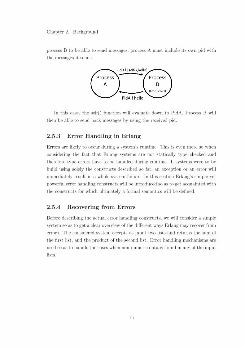
process B to be able to send messages, process A must include its own pid with
the messages it sends.
In this case, the self() function will evaluate down to PidA. Process B will
then be able to send back messages by using the received pid.
2.5.3 Error Handling in Erlang
Errors are likely to occur during a system’s runtime. This is even more so when
considering the fact that Erlang systems are not statically type checked and
therefore type errors have to be handled during runtime. If systems were to be
build using solely the constructs described so far, an exception or an error will
immediately result in a whole system failure. In this section Erlang’s simple yet
powerful error handling constructs will be introduced so as to get acquainted with
the constructs for which ultimately a formal semantics will be defined.
2.5.4 Recovering from Errors
Before describing the actual error handling constructs, we will consider a simple
system so as to get a clear overview of the different ways Erlang may recover from
errors. The considered system accepts as input two lists and returns the sum of
the first list, and the product of the second list. Error handling mechanisms are
used so as to handle the cases when non-numeric data is found in any of the input
lists.
15

Chapter 2. Background
Figure 2.1: SumNProduct System
Diagram 2.1 describes the different ways in which the system may be imple-
mented. It clearly demonstrates that when implementing the system sequentially,
each process is made up of coding surrounded by error handling coding. In the
second version of the system, the system experiences an improvement in efficiency
since the sum and product of the list are being carried out by two separate pro-
cesses. However, just as in the previous case, the process’ coding is cluttered
up with error handling code. This downside is overcome by adopting the design
shown in the last version of the system. In this case, thanks to remote error
handling the system enjoys a higher degree of seperation of concerns since every
process is only responsible of carrying out one particular task either calculating
the sum or the product or recovering from errors. In the following sections, we
will take a closer look into each of the different versions of the system outlining
the constructs that are needed to implement them.
16

Chapter 2. Background
2.5.5 Local Error Handling
2.5.5.1 Exceptions in Erlang
In Erlang there are three classes of exceptions:
• error
• throw
• exit
Exceptions of class error are usually caused due to some unforeseen error
such as calling an undefined functions or attempting to perform arithmetic op-
erations on non-numeric values. throw exceptions are generated by calling the
throw(Reason) built-in function. These types of exceptions are often used within
a try-catch blocks. exit exceptions can be generated by using the exit(Reason)
built-in function. The purpose of this exception is to terminate the process im-
mediately.
2.5.5.2 Try-catch
The try-catch construct has a similar behaviour to the one found in mainstream
programming languages. As mentioned in the previous section, there are three
types of exception classes that can be caught exit, throw and error. When catching
exceptions, the name of the exception class precedes the name of the exception
(errorClass:errorName). For instance, a divide by zero exception which is of class
error or a throw exception can be caught in the following way:
try
10/0
catch
error:badarith-> ’div by 0’
end.
try
throw(stop)
catch
throw:stop -> ’exception caught’
end.
2.5.5.3 SumNProduct - Sequential Version
The Erlang constructs that have been introduced so far, enable us to write the
sequential version of the sumNProduct system.
17

Chapter 2. Background
sum([]) -> 0; product([]) -> 1;
sum([H|T]) -> H+sum(T). product([H|T]) -> H * product(T).
sumNProduct(List1,List2) ->
Sum = try
%% calculate sum of given list
sum(List1)
catch
%% if error occurs return invalid
error:badarith -> invalid
end,
Product = try
%% calculate product of given list
product(List2)
catch
%% if error occurs return invalid
error:badarith -> invalid
end,
[Sum,Product].
Listing 2.1: SumNProduct - Sequential Version
In this case, the try-catch statement will be used so as to recover from er-
rors that might arise if non-numeric data is input. In both cases if an exception
is raised, the system will return the atom invalid. Here it is worth pointing
out that since the two computations have no side-effect actions it is preferable
that they are carried out in parallel. In the next section, the sumNProduct sys-
tem will be implemented using Erlang’s parallel constructs and the two different
implementations will be compared.
2.5.5.4 SumNProduct - Parallel Version
sumNProduct(List1,List2) ->
%% spawn a process to compute the sum of List1
spawn(math,sumProcess,[self(),List1]),
%% spawn another process to compute the sum of List2
spawn(math,productProcess,[self(),List2]),
18

Chapter 2. Background
%% receive the sum value}
receive
[sum,Value1] ->
%% receive the product value
receive
[product,Value2] -> [Value1,Value2]
end
end.
sumProcess(Pid,List) ->
Sum =
try
%% calculate sum of given list
sum(List)
catch
%% if error occurs return invalid
error:badarith -> invalid
end,
%% return Sum to parent process
Pid ! [sum,Sum].
productProcess(Pid,List) ->
Product =
try
%% calculate product of given list
product(List)
catch
%% if error occurs return invalid
error:badarith -> invalid
end,
%% return Product to parent process
Pid ! [product,Product].
Listing 2.3: SumNProduct Example - Parallel Version
The above program will spawn two processes; one process will compute the
sum and another will compute the product. This is done through the following
spawn calls:
%% spawn a process to compute the sum of List1
spawn(math,sumProcess,[self(),List1]),
%% spawn another process to compute the sum of List2
spawn(math,productProcess,[self(),List2]),
Listing 2.4: Spawning new processes
When evaluating these calls, Erlang will first create a new process which will start
evaluating the sumProcess function. Subsequently a new process is created which
will start evaluating the productProcess function. Here, it is important to note
that the sumProcess/productProcess function apart from the list of numbers, will
also expect the pid of the parent process(self() will evaluate down to the parent’s
19

Chapter 2. Background
pid). This pid is needed so that the newly created process will be able to send
back the sum or product of the input list once it completes its computation as
shown hereunder.
Pid ! [sum,Sum]. Pid ! [product,Product].
These are the last statements that are found in the sumProcess/ productProcess
function. One point worth pointing out at this point is that the first element of
the list to be sent(i.e. either sum or product atom) acts as a tag, so that the
parent process will be able to distinguish between the sum and product result.
In fact, when the parent process reads the received results, it will pattern match
against a two element list whose first element is either the sum or product atom.
%% receive the sum value
receive
[sum,Value1] ->
%% receive the product value
receive
[product,Value2] -> [Value1,Value2]
end
end.
Listing 2.5: Receiving Results of Sum and Product
When comparing the parallel version to its sequential counterpart, surely one
major benefit of the parallel one is that it may result in a significant improvement
in performance especially if the input lists are considerably large. Yet, in the
above implementation, errors are still handled locally and therefore code is still
cluttered up with error handling coding. In the next section, we will be introduced
to Erlang’s remote error handling constructs which will make it possible to make
an external process handle any generated errors.
2.5.6 Remote Error Handling
On the strength in Erlang when compared to mainstream programming languages
lies in the fact that it has adopted the notion of remote error handling. In order
to better understand what this term actually refers to let’s consider a very simple
system. In this example the system’s task is to compute the sum of two input
numbers. Error handling mechanisms need to be used in order to handle errors
that might arise due to invalid input data.
20
Chapter 2. Background
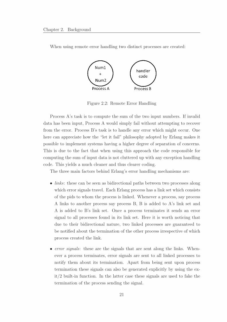
When using remote error handling two distinct processes are created:
Figure 2.2: Remote Error Handling
Process A’s task is to compute the sum of the two input numbers. If invalid
data has been input, Process A would simply fail without attempting to recover
from the error. Process B’s task is to handle any error which might occur. One
here can appreciate how the “let it fail” philosophy adopted by Erlang makes it
possible to implement systems having a higher degree of separation of concerns.
This is due to the fact that when using this approach the code responsible for
computing the sum of input data is not cluttered up with any exception handling
code. This yields a much cleaner and thus clearer coding.
The three main factors behind Erlang’s error handling mechanisms are:
• links : these can be seen as bidirectional paths between two processes along
which error signals travel. Each Erlang process has a link set which consists
of the pids to whom the process is linked. Whenever a process, say process
A links to another process say process B, B is added to A’s link set and
A is added to B’s link set. Once a process terminates it sends an error
signal to all processes found in its link set. Here it is worth noticing that
due to their bidirectional nature, two linked processes are guaranteed to
be notified about the termination of the other process irrespective of which
process created the link.
• error signals : these are the signals that are sent along the links. When-
ever a process terminates, error signals are sent to all linked processes to
notify them about its termination. Apart from being sent upon process
termination these signals can also be generated explicitly by using the ex-
it/2 built-in function. In the latter case these signals are used to fake the
termination of the process sending the signal.
21

Chapter 2. Background
• system processes : processes in Erlang can be classified in two distinct cat-
egories; system processes and non-system processes. The key difference
between the two is how they behave upon receipt of an abnormal error sig-
nal. A system process will translate the error signal into a normal message
and add it to the processes mailbox. On the other hand, a non-system pro-
cess will terminate upon receipt of an abnormal error signal. If a process
wishes to become a system process it can set its flag by using the expression
shown hereafter:
process_flag(trap_exit,true)
Similarly, a process may unset its process flag as follows:
process_flag(trap_exit,false)
By default, the process flag is not set and therefore a process will terminate
immediately on receipt of a process failure notification. If the process flag
has been set to true, the received notification will be added to the process’
mailbox and the process will be notified about a process’ termination by
reading the message from its own mailbox.
Let’s consider a very simple example of how these concepts are actually used.
In the following diagrams links are represented as straight lines and system pro-
cesses are represented as double-lined circles.
Figure 2.3: Erlang system
In the system described in 2.3 process A is linked to both process B and C.
Since all three processes are non-system processes, whenever any of them receives
an error signal they will terminate. Therefore, if process B terminates abnormally,
the following actions will follow.
22

Chapter 2. Background
Figure 2.4: Error propagation
Now let’s consider the same system, modifying Process A to a system process.
Figure 2.5: Error propagation
In this case the error signal sent by Process B is translated into an error mes-
sage and added to Process A’s mailbox. Process C is not notified about Process
B’s termination since there is no direct link between Process B and Process C.
System processes are highly used when building fault-tolerant systems and recov-
ery actions need to be done upon a process failure. For instance, in the above
23

Chapter 2. Background
case, process A could be programmed to restart a copy of Process B again once
it receives process B’s error message.
2.5.6.1 Monitoring
Monitors are very similar in concept to links. Monitors are created by using the
monitor built-in function. For instance, if a process wishes to monitor another
process whose pid is bound to Pid then the monitor(process,Pid) expression
is used. The key difference between monitors and links is that monitors are
unidirectional in contrast to links which are bidirectional. In addition, a monitor
will never terminate abruptly if the process it is monitoring fails. Instead, upon
process termination a message is added to the monitor’s mailbox. To better
understand the difference in behaviours between monitors and links let’s consider
the following diagrams.
Figure 2.6: Links & Monitors - Process Pid1 terminates
Figure 2.5.6.1 demonstrates the different ways in which the linked/monitored
process(i.e. Pid2) behaves when the process creating the link/monitor fails. It
clearly illustrates that since links are bidirectional a failure in Pid1 will imme-
diately be propagated to Pid2. On the other hand, in case 3 since monitors are
24

Chapter 2. Background
unidirectional, Pid2 will not be notified of Pid1’s failure.
Now let’s consider the case when process Pid2 terminates abnormally. As
shown in the diagrams below an error in Pid2, will be immediately propagated
to Pid1 both in the case when using monitors and links.
Figure 2.7: Links & Monitors - Process Pid2 terminates
When comparing the behaviour of linked and monitored processes one ques-
tion that may spring to mind is if it is possible to define monitors in terms of
links as described hereafter:
Process A
monitor(process,Pid2),
....
%%error occurs - reason = stop
Process B
...
Process A
process_flag(trap_exit,true),
link(PidB),
...
%%error occurs - reason = stop
Process B
process_flag(trap_exit,true),
...
Listing 2.6: Monitors & Links
25

Chapter 2. Background
The previous diagrams show that there is an overlapping behaviour between
monitors and links - case 2 and 3 of both figures give the impression that by trap-
ping exit signals, links are able to act just like monitors. However, at this point
it is quite impossible to determine if these two behaviours are truly equivalent or
not. Most surely this is one problem which the defined semantics will be able to
tackle. This is due to the fact that the formal definitions will be able to give us
a clear cut answer to this problem.
2.5.6.2 spawn link, spawn monitor
The spawn link and spawn monitor functions are used to create and link or moni-
tor the process as one atomic action. Perhaps here one might ask if the spawn link
construct is simply syntactic sugaring for spawn() followed by link().
spawn_link(module,function,[args]), ?⇔
Pid = spawn(module,function,[args]),
link(Pid),
Listing 2.7: spawn link & spawn() + link ()
The only possible way to answer such a problem is through a formal semantic
definition of these constructs.
2.5.6.3 Explicit Error Signals
So far, we have seen that the primary source of error signals is the failure of a
linked/monitored process. An additional way how error signals can be generated
is by using the exit(pid,reason) built-in function(In the following sections, this
function will be referred to exit/2 so as to be able to dinstinguish this function
from the exit function described in Section 2.5.5.1). This construct expects two
arguments, the Pid to whom the error signal is to be sent and the reason describing
the cause of the error. The behaviour of the receiving process depends mainly on
two things:
- The reason passed as the second argument
- The recipient’s process flag
If the reason is equal to kill, the recipient process will terminate immediately
with reason killed, irrespective if it is trapping exit signals or not. Otherwise,
the behaviour of the recipient process will be determined by whether or not the
26
Chapter 2. Background
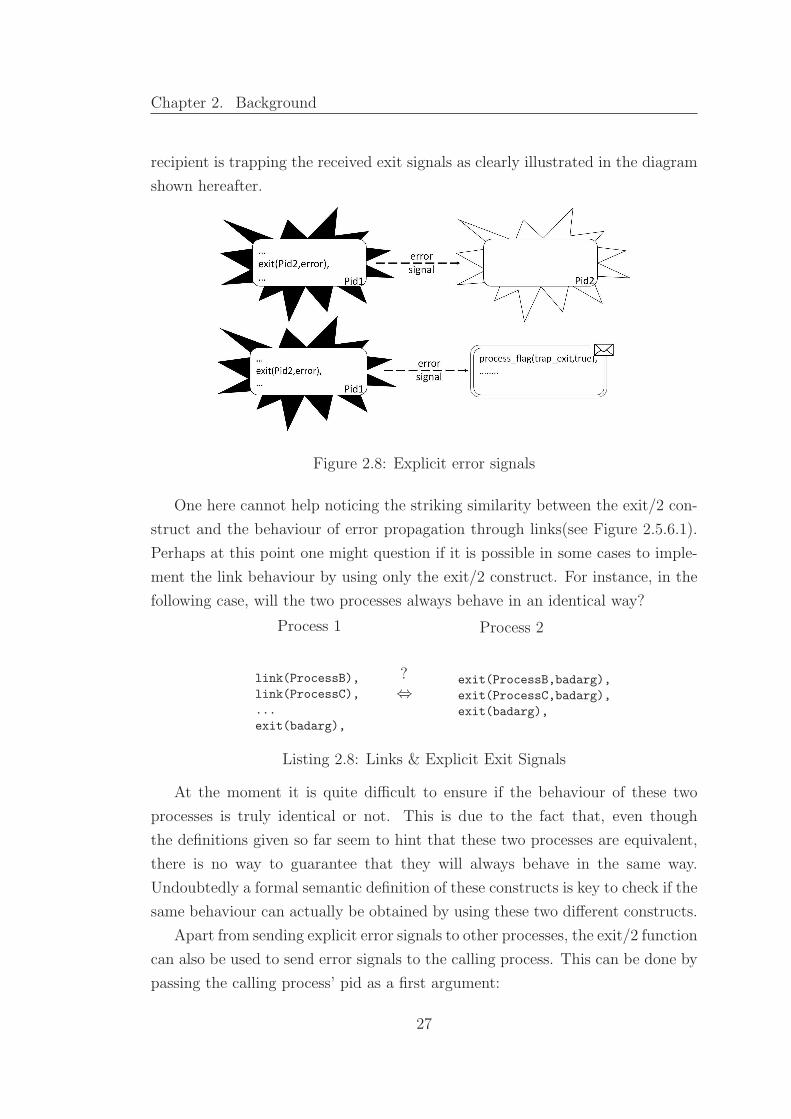
recipient is trapping the received exit signals as clearly illustrated in the diagram
shown hereafter.
Figure 2.8: Explicit error signals
One here cannot help noticing the striking similarity between the exit/2 con-
struct and the behaviour of error propagation through links(see Figure 2.5.6.1).
Perhaps at this point one might question if it is possible in some cases to imple-
ment the link behaviour by using only the exit/2 construct. For instance, in the
following case, will the two processes always behave in an identical way?
Process 1
link(ProcessB),
link(ProcessC),
...
exit(badarg),
?⇔
Process 2
exit(ProcessB,badarg),
exit(ProcessC,badarg),
exit(badarg),
Listing 2.8: Links & Explicit Exit Signals
At the moment it is quite difficult to ensure if the behaviour of these two
processes is truly identical or not. This is due to the fact that, even though
the definitions given so far seem to hint that these two processes are equivalent,
there is no way to guarantee that they will always behave in the same way.
Undoubtedly a formal semantic definition of these constructs is key to check if the
same behaviour can actually be obtained by using these two different constructs.
Apart from sending explicit error signals to other processes, the exit/2 function
can also be used to send error signals to the calling process. This can be done by
passing the calling process’ pid as a first argument:
27

Chapter 2. Background
exit(self(), Reason)
This generated exit signal may cause the calling process to terminate with reason
Reason. One question that springs to mind here is if the behaviour of self-sent
exit signals is equivalent to the exit(Reason) statement. This is due to the fact
that the exit(Reason) expression may also cause the process to terminate with
reason Reason (see Section 2.5.5.1).
exit(reason)?⇔
exit(self(),reason)
Listing 2.9: exit(Reason) & exit(self(),Reason)
Certainly, this is yet another interesting problem that the formal semantics should
be able to solve.
2.5.6.4 SumNProduct - Remote Error Handling
sumNProduct(List1,List2) ->
%% set process flag to true to trap any error signals
process_flag(trap_exit,true),
%% spawn process to compute Sum
SumPid = spawn_link(math,sumProcess,[self(),List1]),
%% spawn process to compute Product
ProductPid = spawn_link(math,productProcess,[self(),List2]),
%% receive Sum and Product value
Sum = receiveValue(SumPid,sum),
Product = receiveValue(ProductPid,product),
[Sum,Product].
%% calculates sum of List
sumProcess(Pid,List) -> Pid ! [sum,sum(List)].
%% calculates product of List
productProcess(Pid,List) -> Pid ! [product,product(List)].
28

Chapter 2. Background
%% check if the linked process terminated normally or not
receiveValue(Pid,Tag)->
receive
%% if linked process terminated normally
%% then read result from mailbox
{’EXIT’,Pid,normal} ->
receive
[Tag,Value] -> Value
end;
%% otherwise if process terminated abnormally
%% return invalid
{’EXIT’,Pid,{badarith,Stack}} -> invalid
end.
Listing 2.11: SumNProduct - Remote Error Handling
In this version of the sumNProduct system, Erlang will first set the pro-
cess flag to true. This is done so that the process will be able to trap any errors
that might occur in any of the processes with whom it will become linked later
on. Erlang will then spawn link two separate processes; one to calculate the sum
and the other to calculate the product.
process_flag(trap_exit,true),
SumPid = spawn_link(math,sumProcess,[self(),List1]),
ProductPid = spawn_link(math,productProcess,[self(),List2]),
Listing 2.12: Parent process
Here, it is worth pointing out that since both processes are linked and the
process flag is set to true, the parent process will receive an exit notification mes-
sage once the linked processes have terminated. If the linked process completed
its task normally, the parent process will receive an {’EXIT’,Pid, normal} mes-
sage. On the other hand, if the linked process terminated abnormally due to
non-numeric data it will receive a {’EXIT’,Pid,{badarith, Stack}} message.
In both cases the Pid, refers to the pid of the terminated process. After creating
the two processes, the parent process will then suspend until it receives the results
of the two processes.
29
Chapter 2. Background
receiveValue(Pid,Tag)->
receive
{’EXIT’,Pid,normal} ->
receive
[Tag,Value] -> Value
end;
{’EXIT’,Pid,{badarith,Stack}} -> invalid
end.
Listing 2.13: Receiving Results from processes
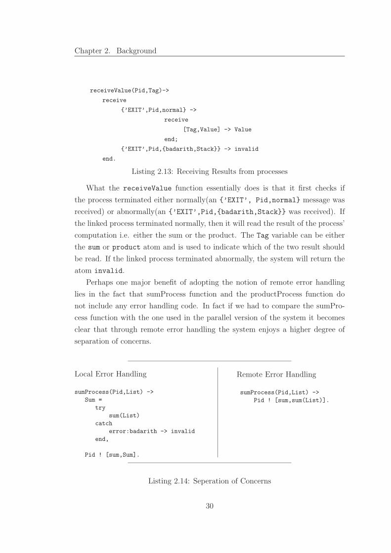
What the receiveValue function essentially does is that it first checks if
the process terminated either normally(an {’EXIT’, Pid,normal} message was
received) or abnormally(an {’EXIT’,Pid,{badarith,Stack}} was received). If
the linked process terminated normally, then it will read the result of the process’
computation i.e. either the sum or the product. The Tag variable can be either
the sum or product atom and is used to indicate which of the two result should
be read. If the linked process terminated abnormally, the system will return the
atom invalid.
Perhaps one major benefit of adopting the notion of remote error handling
lies in the fact that sumProcess function and the productProcess function do
not include any error handling code. In fact if we had to compare the sumPro-
cess function with the one used in the parallel version of the system it becomes
clear that through remote error handling the system enjoys a higher degree of
separation of concerns.
Local Error Handling
sumProcess(Pid,List) ->
Sum =
try
sum(List)
catch
error:badarith -> invalid
end,
Pid ! [sum,Sum].
Remote Error Handling
sumProcess(Pid,List) ->
Pid ! [sum,sum(List)].
Listing 2.14: Seperation of Concerns
30

Chapter 2. Background
Through this simple example it becomes clear how remote error handling en-
ables us to write fault-tolerant systems which are not cluttered up with exception
handling coding. As a result, the number of lines related to error recovery within
the system has been reduced. Even though the reduction in this simple system
was minimal, one can easily imagine the significant reduction that can be achieved
when this concept is applied to larger parallel systems. In fact in his book, Ce-
sarini claimed that a particular system which was formerly implemented in C++
experienced an amazing 85% reduction in code when implemented in Erlang. One
of the main contributors to this dramatic reduction was Erlang’s error handling
mechanisms since as stated in [12] “ 27% of the C++ code consisted of defensive
programming”. It is a well-known known fact that the number of bugs within
a system is directly proportional to the number of lines of code. Therefore, this
reduction plays an important role in reducing drastically the presence of bugs
within a system.
2.6 Conclusion
This chapter has taken a closer look at the main constructs incorporated within
Erlang. A simple example was used to acquaint us with Erlang’s error handling
mechanisms. It was illustrated how Erlang enables us to handle errors locally
through the try-catch construct similar to the way other conventional program-
ming languages handle errors. The chosen example, was also implemented using
Erlang’s remote handling mechanisms. This helped to bring out certain benefits
that remote error handling has over local error handling namely reduction in lines
of code and a higher degree of separation of concerns.
However, one recurrent dilemma when describing these Erlang constructs was
if some constructs could actually be implemented in terms of other constructs.
One particular case was for instance that of monitors and trap-exit links. In ad-
dition, even though the sumNProduct system was implemented in different ways
there was no way one could actually guarantee that the system really maintained
its semantic definition. The next chapter attempts to solve these problems by
presenting a formal semantic definition for these constructs. These definition will
make it possible to indicate if two syntactically different systems have similar
behaviour or not.
31

3. Formal Semantics
3.1 Introduction
The main focus of this chapter is to get a better understanding of Erlang’s error
handling behaviour by presenting a formal model for Erlang’s error handling
constructs. In order to better appreciate the usefulness of this model, a number
of Erlang systems are considered and the behaviour of these systems is described
in terms of the model.
3.2 The need for Formal Semantics in Erlang
More often than not, the semantics of a language are more likely to be defined
through informal description rather than through a formal one. However, lately
more emphasis is being put on formal semantics, mainly due to the number
of benefits they offer over their informal counterparts. In this section, the main
drawbacks of using informal semantics to describe the behaviour of Erlang’s error
handling constructs are discussed so as to better understand the need of a formal
model.
One major downside of using informal descriptions stems from the fact that
they leave scope for ambiguity and therefore, as clearly shown in the previous
chapter, they are not able to show if two different programs will actually behave
in the same way or not. In contrast, formal semantics are able to present an un-
ambiguous and more accurate description of a system’s behaviour. Consequently,
when using these semantics it becomes much more straightforward to show if the
behaviour of two different programs is actually equivalent or not.
32

Chapter 3. Formal Semantics
Another, drawback of informal descriptions is that in certain cases, they may
fall short of accurately describing how the different Erlang constructs might in-
teract. As a result, it may become relatively challenging to understand a system’s
behaviour through these semantics. This is even more so, when considering the
fact that due to the parallel nature of Erlang systems, the interleaving of pro-
cesses may result in different behaviour at consecutive executions of the same
system. Thus, describing how parallel systems may behave by using informal
semantics may result in really lengthy and cumbersome descriptions. On the
other hand, through formal semantics it becomes much easier to reason about
the behaviour of parallel systems. This is because, from their very nature they
are able to provide concise but detailed descriptions of how a particular system
might behave.
3.3 Current Formal Semantics in Erlang
Due to the fact that Erlang was conceived in industry, it was primarily defined
in terms of its implementation[13]. However, given the significant role that for-
mal semantics play in reasoning about the behaviour of systems, it was evident
that defining such semantics for Erlang was key in understanding soundly the be-
haviour of Erlang programs. This is even more so, when considering the fact that
Erlang systems are highly dynamic and concurrent and therefore, they tend to
become quite challenging to fully reason about their behaviour. Erlang’s current
formal semantics can be classified in three categories[16]:
• functional semantics
• process semantics
• node semantics
The functional semantics, as the name itself implies, deals with the functional part
of Erlang such as pattern matching and function evaluation whilst the process
semantics deals with the process rules for instance, process termination, message
passing and links. The semantics defined in these two categories, are used to
describe the behaviour of systems found on a single machine[14]. On the other
hand, the behaviour of multi-node systems can be described through the node
semantics[13]. The term multi-node system refers to the fact that a particular
33
Chapter 3. Formal Semantics
Erlang system may sometimes be composed of multiple runtime systems commu-
nicating with each other. In Erlang each of these runtime systems is called a node.
Multi-node systems are oftenly used when implementing distributed systems.
3.3.1 Differences Between Current Semantics and Defined
Model
One of the most noticeable difference between the current semantics and the de-
fined model lies in the fact that whereas all current formal semantics of Erlang[14,
13] are defined by using an LTS semantics in this project the formal rules are de-
fined by using a reduction semantics. By adopting this approach, the semantics
are able to provide a clearer picture of how communication between processes is
carried out. This is because, when using a reduction semantics both the sender
and receiver of a signal are included in the rule definition. As a result, it becomes
easier to see how a particular action has effected the receiving process. Addition-
ally, the syntax of the reduction semantic definitions is somewhat closer to the
way in which these semantics may be implemented through an evaluator.
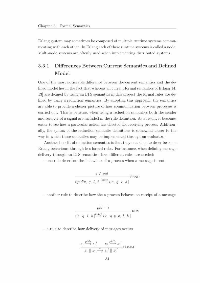
Another benefit of reduction semantics is that they enable us to describe some
Erlang behaviours through less formal rules. For instance, when defining message
delivery through an LTS semantics three different rules are needed:
- one rule describes the behaviour of a process when a message is sent
i 6= pidSEND
i[pid!v, q, l, b ]pid!v−→ i[v, q, l, b ]
- another rule to describe how the a process behaves on receipt of a message
pid = iRCV
i[e, q, l, b ]pid?v−→ i[e, q ++ v, l, b ]
- a rule to describe how delivery of messages occurs
s1pid!v−→ s1
′ s2pid?v−→ s2
′
COMMs1 || s2
τ−→ s1
′ || s2′
34

Chapter 3. Formal Semantics
In contrast, when describing the delivery of messages through reduction semantics
only one rule is used:
i 6= pidSEND
i[j!v, q, l, b ] || j[e, qj, lj , bj ] −→
i[v, q, l, b ] || j[e, qj++ v, lj, bj ]
Another fact worth mentioning with respect to the current Erlang semantics, is
that the formal semantic definition of certain mechanisms is somewhat inaccurate
since it does not faithfully mirror the behaviour of actual Erlang. A case in point
is the way the current semantics defines the behaviour of Erlang when a link
failure occurs. According to these semantics whenever a process attempts to
link to a terminated process, an exit signal is immediately sent to the process
attempting to create the link. However, as clearly described in [18] a link failure
may not necessary cause the system to behave in this way. The model presented
in this chapter addresses this inaccuracy and defines a more accurate description
of how Erlang behaves in the case of link failure.
The current semantics also fall short of describing the way a process may
behave when it sends an explicit exit signal to itself(by using the exit(self(),
Reason) expression). In fact, the current semantics are only able to describe
soundly the way a system behaves when an explicit exit signal is sent to another
different process. In the formal semantics described in this project some rules
were defined to faithfully describe the way a process behaves when an explicit
exit signal is sent to itself(see section 3.11.4).
Another improvement over the current semantics is that the presented model
is able to describe both the linking and monitoring mechanisms in Erlang whereas
the current semantics are only able to describe the linking behaviour. It is im-
portant to note that even though in [3] it was claimed that monitors can be
implemented in terms of links, in truth there exist some subtle differences be-
tween the two mechanisms. As a result, implementing monitors in terms of links
may not be as easy as it might seem. This fact is discussed in more depth in sec-
tion 3.11.5, where a simple example is considered to highlight the main differences
that exist between monitoring and linking.
The next sections presents the formal model defined in this project whose
aim is to accurately describe the behaviour of Erlang systems in the presence of
errors.
35
Chapter 3. Formal Semantics
3.4 Erlang System
Here a formal description of an Erlang system will be given together with some
fundamental rules that will be used as the foundation for the defined semantics.
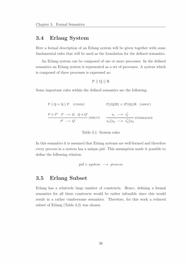
An Erlang system can be composed of one or more processes. In the defined
semantics an Erlang system is represented as a set of processes. A system which
is composed of three processes is expressed as:
P || Q || R
Some important rules within the defined semantics are the following:
P || Q ≡ Q || P (COMM) P||(Q||R) ≡ (P||Q)||R (ASSOC)
P ≡ P ′ P −→ Q Q ≡ Q′
STRUCT
P ′ −→ Q′
s1 −→ s′1INTERLEAVE
s1||s2 −→ s′1||s2
Table 3.1: System rules
In this semantics it is assumed that Erlang systems are well-formed and therefore
every process in a system has a unique pid. This assumption made it possible to
define the following relation:
pid× system −→ process
3.5 Erlang Subset
Erlang has a relatively large number of constructs. Hence, defining a formal
semantics for all these constructs would be rather infeasible since this would
result in a rather cumbersome semantics. Therefore, for this work a reduced
subset of Erlang (Table 3.2) was chosen.
36

Chapter 3. Formal Semantics
digit :: = 0 | · · · |9uppercase :: =A| · · · |Zlowercase :: = a | · · · |zdigitletter :: = digit|uppercase|lowercase| |@
number :: = digit+
unquotedatom :: = lowercase digitletter∗
quotedatom :: = ′(digitletter|whitespace)+ ′
atom :: = unquotedatom|quotedatomvar :: = uppercase digitletter∗
value(v) :: = atom
| int
| pid
| [ ]
compound value (cv) :: = v|[cv1|cv2]
expression (e) :: = v | [e1|e2]| var
| built-in function
| e1, e2| case e of m end| try e catch m end| receive m end| e1!e2
pattern(p) :: = cv | var | [p1|p2]matchPtrn (m) :: = p1 → e1; · · · ; pn → en
built-in functions(b) :: = self()| spawn(e, e, e)| link(e)| monitor(e, e)| spawn link(e, e, e)| spawn monitor(e, e, e)| process flag(e, e)| error(e)| throw(e)| exit(e)| exit(e, e)
Table 3.2: Erlang’s subset
When expressing the formal definitions of Erlang’s constructs some minor
syntactic modifications were made to Erlang’s syntax. This was done so as to
represent expressions in a neater way. These modifications are primarily the
following:
- a sequence of Erlang expressions will be delimeted by a · instead of a comma.
37

Chapter 3. Formal Semantics
This is because the comma will act as a delimeter for separating the different
elements in the tuple representing an Erlang process.
- the concept of modules will not be present in the defined semantics since the
notion of modules does not in any way affect Erlang’s error handling behaviour.
As a result, built-in functions such as spawn, spawn link and spawn monitor do
not expect the module name parameter.
3.6 Contextual Rules
The formal rules presented in this project are only able to describe the behaviour
of expressions for the case when all parameters of an expression have already been
evaluated down to a value. As a result, the reduction context rules are necessary
in order to define the way a subexpression is evaluated with respect to a bigger
context.
i[e, m, l, f ] −→ i[e′, m′, l′, f ′ ]CONTEXT0
i[c[e], m, l, f ] −→ i[c[e′], m′, l′, f ′ ]
i[e, m, l, f ] −→ i[ex, m′, l′, f ′ ]CONTEXT1
i[c[e], m, l, f ] −→ i[ex, m′, l′, f ′ ]
Table 3.3: Contextual rules
A reduction context, c[] defines a subexpression position such that, if a subex-
pression e performs an action and reduces down to e1, than the whole expression
can perform the same action and only the subexpression e is changed. For in-
stance, when evaluating the following case statement
case e of m end
the model will first try to reduce expression e. If e reduces down to e1, then the
whole expression reduces down to
case e1 of m end.
38

Chapter 3. Formal Semantics
c[·] ::= ·
| funName(..., vn−1, c[·], en+1, ...) n > 0
| [..., vn−1, c[·], en+1] n > 0
| c[·]!e | v!c[·]
| case c[·] of mt end
What the c[·] definition essentially states is that when reducing a function call
Erlang will evaluate the functions paramenters from left to right. Elements in
a list are also evaluated from left to right. When evaluating a send statement,
Erlang will first evaluate the expression on the left hand side, and subsequently
it will start evaluating the expression found after the ! operator. The last part
of the definition describes the fact that when evaluating a case statement Erlang
will first evaluate the expression found between the case and of keywords.
3.7 Erlang Process
In this section the notion of an Erlang process is formalised. In this semantics
processes may be in one of two states, either alive or terminated. Here, it is worth
mentioning the fact that terminated processes cannot be considered as dead or
useless processes. This is due to the fact that terminated processes will still have
some tasks to carry out such as informing all processes found in their link set
about their termination. Additionally, terminated processes are also used when
defining the behaviour of the linking mechanism.
A live process is represented as
p[e,m, l, f ]
pid(p) - a unique process identifier
expression(e) - the expression the process is executing
mailbox(m) - a list of received messages that are waiting to be read
links(l) - the set of pids to which the process is linked
flag(f) - a boolean value indicating if a process is trapping exit
signals or not
39

Chapter 3. Formal Semantics
A terminated process is expressed as
p[r,l]
pid(p) - a unique process identifier
reason(r) - reason describing process termination
links(l) - the set of pids found in the link set
A live Erlang process may terminate either normally or abnormally.
TERM0
i[v, m, l, f ] −→ i[normal, l]
TERM1
i[ex, m, l, f ] −→ i[reason(ex), l]
Table 3.4: Process Termination Rules
TERM0 states that when a process completes its task, it will terminate with
reason normal. Otherwise, the reason will describe the error that caused the
process to terminate(TERM1).
3.8 Case Statement
∃I.((result v mtI e) ∧ ∀J.J < I ⇒ ¬(matches v mtJ))CASE0
i[case v of mt end, m, l, f ] −→ i[e, m, l, f ]
∀I.¬(matches v mtI)CASE1
i[case v of mt end, m, l, f ] −→ i[error:{case clause, v}, m, l, f ]
Table 3.5: Case rules
Before describing what these rules state, the matches and result functions will be
defined. (The definition of these two function is very similar to the one defined
in [14].)
The matches function is defined as:
matches v (p → e) , ∃V .(v = p{V /fv(p)})
40

Chapter 3. Formal Semantics
The matches function is given two parameters, a value(v) and a (pattern →
expression). This function returns true if pattern p is identical to valuev once
the substitution(p{V /fv(p)}) is done. Two functions used in this substitution
are the:- V : returns all the values found in v. For example, if v = [1, 2, 3, 4] then
V = 1, 2, 3, 4.
- fv(p) : returns all the free variables found in pattern p. For instance,
fv([a,B, c,D]) = [B,D].
What the p{V /fv(p)} substitution essentially does is that it replaces variables
according to their position in the list. For instance, let’s consider the case when:
v = [1, 2, 3, 4] p = [a,X, c, Y ]
V = 1, 2, 3, 4 fv(p)= X, Y
In this case, when evaluating p{V /fv(p)}, free variable X, the second element
of p, is replaced by 2, the second element of v, and free variable Y, the fourth
element of p is replaced by 4, the fourth element of v:
p{V /fv(p)} = [a, 2, c, 4]
If p and v have different arities no replacements are done.
The result function is defined as:
result v (p → e) e′ , ∃V .(v = p{V /fv(p)} ∧ e′ = e{V /fv(p)})
The result function is very similar to the matches function. The only difference
is that this function has an extra parameter e′. This parameter represents the
corresponding body of the pattern which successfully pattern matched against
the given value. For instance, in the following case, this predicate will return
true:
v = [text, hello]
p → e= [text, V alue] → V alue
e′ = hello
41

Chapter 3. Formal Semantics
Now let’s move on to describe the behaviour of the case statement as defined
in these rules. The first rules states that the system will try to pattern match
the value against the patterns found in mt(CASE0). The patterns in mt are
sequentially matched against the value v found between the case and of keywords.
The described reduction step is done if
∃I.((result v mtI e) ∧ ∀J.J < I ⇒ ¬(matches v mtJ))
What the above predicate essentially states is that a case statement will return
the expression e if
- one of the elements in mt, say (p1 → e), consists of a pattern p1
that can be successfully pattern matched against v and
- all the elements prior to (p1 → e) fail to pattern match against v
Therefore, if we evaluate the following case statement according to CASE0:
case [a,b,c] of
[X,Y] -> first;
[X,Y,Z] -> second;
X -> third
end.
the system first tries to pattern match [a, b, c] against [X, Y ] and it fails. Sub-
sequently, it attempts to pattern match [a, b, c] against [X, Y, Z] and it succeeds.
As a result, it returns the atom second. Note that the value [a, b, c] can be also
successfully pattern matched against the last pattern X. However, the defined
rule states that the case statement should always return the body of the first
pattern against which [a, b, c] is successfully pattern matched.
The second rule states that if the value fails to pattern match against any of
the patterns in mt(∀I.¬(matches v mtI)), then an exception is raised(CASE1).
42

Chapter 3. Formal Semantics
3.9 Local Error Handling - try-catch
TRY0
i[try v catch mt end, m, l, f ] −→ i[v, m, l, f ]
i[e, m, l, f ] −→ i[e′, m′, l′, f ′ ]TRY1
i[try e catch mt end, m, l, f ] −→ i[try e′ catch mt end, m′, l′, f ′ ]
i[e, m, l, f ] −→ i[ex, m, l, f ]
∃I.((result ex mtI e′) ∧ ∀J.J < I ⇒ ¬(matches ex mtJ))TRY2
i[try e catch mt end, m, l, f ] −→ i[e′, m, l, f ]
∀I.¬(matches ex mtI)
i[e, m, l, f ] −→ i[ex, m, l, f ]TRY3
i[try e catch mt end, m, l, f ] −→ i[ex, m, l, f ]
Table 3.6: Rules for local error handling
These rules describe that Erlang will first try to evaluate the expression between
the try and catch statement(TRY1). If this expression evaluates down to a value
than that value is returned(TRY0). If the expression raises an exception, the
system will try to pattern match the exception against the patterns found in mt
and if the exception pattern matches, the corresponding error handling code is
returned(TRY2). Otherwise, if the exception is not caught the try expression will
return the raised exception. (TRY3).
3.9.1 sumNProduct Example(Sequential version)
Using the rules defined so far it is now possible to get a step-by-step description
of how the example explained in section 2.5.5.3 is evaluated. Here, only the
reduction steps related to the evaluation of sum(List1)will be shown.
try sum(List1) catch error:badarith -> 0 end,...
The evaluation of
... try product(List2) catch error:badarith -> 0 end.
43

Chapter 3. Formal Semantics
is almost identical. First, let’s consider the case when the input list is the numeric
list [12,5]. By using rule TRY1 the system will first evaluate sum([12,5]) :
i[try sum([12, 5]) catch error :badarith → invalid end · e1, ε, ∅, false]
−→ i[try 12 + sum([5]) catch error :badarith → invalid end · e1, ε, ∅, false] (TRY1)
−→ i[try 12 + 5 catch error :badarith → invalid end · e1, ε, ∅, false] (TRY1)
where e1 = try product([12, 5]) catch error :badarith → invalid end·
[Sum,Product]
Since the expression between the try and catch block evaluated down to a value,
by rule TRY0 the whole try-catch construct will evaluate down to 17.
−→ i[try 17 catch error :badarith → invalid end · e1, ε, ∅, false] (TRY1)
−→ i[17 · e1, ε, ∅, false] (TRY0)
−→ i[e1, ε, ∅, false] (SEQ1)
The system will then continue to evaluate e1.
One here can appreciate that the defined rules make it possible to ascertain
that the system will always return the sum of the input list whenever valid num-
bers are input since there does not exist any other possible sequences of steps
that may lead to a different result.
Now let’s consider the case where the input list contains a non-numeric value;
[a,12]. As in the previous case the system will first evaluate the expression found
within the try catch block:
i[try sum([a, 12]) catch error :badarith → invalid end · e1, ε, ∅, false]
−→ i[try a+ sum([12]) catch error : badarith → invalid end · e1, ε, ∅, false] (TRY1)
−→ i[try a+ 12 catch error :badarith → invalid end · e1, ε, ∅, false] (TRY1)
where e1 = try product([12, 5]) catch error :badarith → invalid end·
[Sum,Product]
44

Chapter 3. Formal Semantics
When the system attempts to add a to 12 a badarith exception is raised:
−→ i[try error :badarith catch error :badarith → invalid end · e1, ε, ∅, false] (TRY1)
The generated exception is caught and therefore the output of this computation
will be the atom invalid.
−→ i[invalid · e1, ε, ∅, false] (TRY2)
−→ i[e1, ε, ∅, false] (SEQ1)
The system will then continue to evaluate e1.
3.10 Parallel Erlang
fresh(j)SPAWN
i[spawn(f, args), m, l, f ] −→
i[j, m, l, f ]||j[f(args), ε, ∅, false ]
i = jSEND0
i[j!v, m, l, f ] −→ i[v, m++ v, l, f ]
i 6= jSEND1
i[j!v, mi, li, fi ] || j[ej , mj , lj , fj ] −→
i[v, mi, li, fi ] || j[ej , mj ++ v, lj , fj ]
i 6= jSEND2
i[j!v, mi, li, fi ] || j[reason, {pids}] −→
i[v, mi, li, fi ] || j[reason, {pids}]
∃I.((result v mtI e) ∧ ∀J.J < I ⇒ ¬(matches v mtJ))RCV
i[?mt, m1 ++ v ++m2, li, fi ] −→ i[e, m1 ++m2, l, f ]
Table 3.7: Process rules
45

Chapter 3. Formal Semantics
The SPAWN rule states that whenever a new process is created, its identifier
must be unique(fresh(j)). It also illustrates that the new process will have an
empty mailbox and link set. Additionally, by default it will not be trapping any
exit signals since its process flag is set to false.
With regards to message delivery, it was assumed that all messages arrive in
their destination instantaneously. In fact, in actual Erlang when dealing with
single-node systems it is guaranteed message delivery is immediate. The instan-
taneous message delivery is described by the three SEND rules. SEND0 describes
the fact that when a process sends a message to itself, the message is immediately
appended to the process’ mailbox. When a process sends a message to another
process, say process j then this message is appended immediately to process j’s
mailbox(SEND1). The last send rule describes the fact that when a message is
sent to terminated process j then the message is not appended to process j’s
mailbox(SEND2).
What the RCV rule states is that the receive construct will attempt to pattern
match sequentially the patterns found in mt with the messages found in the
mailbox. The body of the first pattern to pattern match against one of the
messages in the mailbox will be returned. This fact is described through the
following predicate:
∃I.((result v mtI e) ∧ ∀J.J < I ⇒ ¬(matches v mtJ))
For this predicate to hold:
- one of the patterns in mt must pattern match against the mes-
sage v which is currently found in the process’ mailbox described as
[m1 ++ v ++m2]
- all messages found in the mailbox prior to v i.e. in [m1] do not pattern
match against any of the patterns found prior to mtI .
Once a message has been pattern matched it is removed from the mailbox. Note
that if no messages pattern match against any of the patterns in mt than the
system will block. This is the main reason why there is no reduction rule defined
to cater for this particular case.
46

Chapter 3. Formal Semantics
3.10.1 sumNProduct Example(Parallel Version)
Through these rules, it is now possible to describe the behaviour of the sumN-
Product system(parallel version). In this version, two seperate processes are used
to calculate the sum and product of the input lists. We will first consider the
case when two valid lists are input; for this example both input lists are [12,5].
Firstly, the system will spawn a new process whose task is to calculate the
sum of [12,5]. The pid of the newly created process, in this case j will be returned
to the parent process i.
i[spawn(sumProcess, [i, [12, 5]]) · e1, ε, ∅, false]
−→ i[j · e1, ε, ∅, false] || j[sumProcess(i, [12, 5]), ε, ∅, false] (SPAWN)
−→ i[e1, ε, ∅, false] || j[sumProcess(i, [12, 5]), ε, ∅, false] (SEQ1)
where e1 = spawn(productProcess, [i, [12, 5]]) ·
?[sum, V alue1] →?[product, V alue2] → [V alue1, V alue2].
Process i will then spawn another process whose task is to calculate the product
of [12,5].
−→ i[k · e2, ε, ∅, false] || k[productProcess(i, [12, 5]), ε, ∅, false] ||
j[sumProcess(i, [12, 5]), ε, ∅, false] (SPAWN)
where e2 = ?[sum, V alue1] →?[product, V alue2] → [V alue1, V alue2].
Once the sum of the list has been calculated, the sumProcess functions will eval-
uate the i![sum, 17] expression. When evaluating this expression, process j will
send a message containing the sum result to process i. The sent message will be
appended to process i’s mailbox.
≡ j[i![sum, 17]), ε, ∅, false] || i[e2, ε, ∅, false] || sk
−→ j[[sum, 17], ε, ∅, false] || i[e2, [[sum, 17]], ∅, false] || sk (SEND1)
where sk = k[productProcess(i, [12, 5]), ε, ∅, false]
Similarly, once the product of the list has been calculated, the productProcess
47

Chapter 3. Formal Semantics
functions will evaluate the i![product, 60] expression. When evaluating this ex-
pression, process k will send the product result to process i. This will be also
appended to process i’s mailbox.
≡ k[i![product, 60]), ε, ∅, false] || i[e2, ε, ∅, false] || sj
−→ k[[product, 60], ε, ∅, false] ||
i[e2, [[sum, 17], [product, 60]], ∅, false] || sj (SEND1)
where sj = j[[sum, 17], ε, ∅, false]
Process i will then start reading the received messages. It will first read the sum
Value. Once this message is read it will be removed from the mailbox.
≡ i[?[sum, V alue1] →?[product, V alue2] →, [[sum, 17], [product, 60]], ∅, false]
|| sj || sk
−→ i[?[product, V alue2] → [17, V alue2], [[product, 60]], ∅, false] || sj || sk
(RCV)
Subsequently, process i reads the received product result. Once this message is
read it is also removed from the mailbox. The system will then return a list
containing the sum and product of the input lists.
−→ i[[17, 60], ε, ∅, false] || sj || sk (RCV)
The above steps show only one possible sequence of reductions that leads to
the expected output i.e.[17,60]. One fact worth pointing out here is that in truth
there a several other possible interleavings which can lead to the same output. For
instance, process j could have sent the [sum,17] message before process i spawned
process k. In fact, even though this system consists only of three processes
there are relatively many different possible interleavings. Nonetheless, the defined
semantic rules enable us to check that given the same input there does not exist
any possible interleaving that may lead to a different output. Here one can
appreciate even more how such simple rules have in actual fact paved the way to
show such an essential fact.
In order to check if the parallel version of sumNProduct is semantically equiv-
48

Chapter 3. Formal Semantics
alent to the sequential version we will need to check the case when invalid data is
passed. Though it will not be illustrated here(since the reduction steps are highly
similar to the ones described in the sequential version of the sumNProduct exam-
ple), through these semantics it is possible to show that in fact the system will
always evaluate down to [invalid, invalid] when given non-numeric data. There-
fore, it can be concluded that the parallel version of sumNProduct is semantically
equivalent to its sequential version.
3.11 Remote Error Hadling
3.11.1 Links and System Processes
LINK0i[link(j), mi, li, fi ] || j[ej , mj , lj , fj ] −→
i[true, mi, li ∪ {j}, fi ] || j[ej , mj , lj ∪ {i}, fj ]
f = trueLINK1
i[link(j), m, l, f ] || j[v, l] −→
i[true, m++ [′EXIT ′, j, noproc], l, f ] || j[v, l]
f = falseLINK2
i[link(j), m, l, f ] || j[v, l] −→
i[error:noproc, m, l, f ]||j[v, l]
PROC FLAGi[process flag(trap exit, f lag1), m, l, f2 ] −→
i[f2, m, l, f lag1 ]
Table 3.8: Process rules for linking and system processes
As already described in section 2.5.6 links are the underlying factor behind Er-
lang’s remote handling mechanisms. These three rules bring to light the fact that
the link expression can be also used as a ping. This is because the link(Pid)
expression is able to indicate if the process identified by Pid is alive(LINK0) or
dead(LINK1 or LINK2). Rule LINK0 describes Erlang’s behaviour when a pro-
cess successfully links to another process. Here, it is worth mentioning the fact
that since in this semantics links are expressed as a set, it is ensured that when-
ever a process attempts to link to a process which is already found in its link set
49

Chapter 3. Formal Semantics
nothing actually happens. This guarantees that the defined rules are faithful to
the behaviour of actual Erlang.
The last two rules describe Erlang’s behaviour when a process tries to link
to a terminated process. LINK1 describes link failure when the process calling
link is trapping exit signals i.e. the process flag is set to true. In this case a link
failure will result in a message to be appended to the calling process’ mailbox.
LINK2 describes the case when the calling process is not trapping exit signals.
In this case a link failure evaluate down to an exception. Interestingly enough all
semantics which have attempted to describe Erlang’s error handling mechanisms
so far, always describe a link failure in the following way:
Figure 3.1: Link Failure as described by Current Semantic Definitions
As shown in the above diagram, according the these semantics a link failure
will always trigger the terminated process to send an exit signal with reason
noproc. Consequently, since process A is not trapping exit signals, the sent signal
will cause process A to terminate with reason noproc.
However, according to Erlang’s reference manual [23], a link failure may result
in either of the following:
- If the calling process is not trapping exits, and checking Pid is cheap
– that is, if Pid is local – link/1 fails with reason noproc.
- Otherwise, if the calling process is trapping exits, and/or Pid is
remote, link/1 returns true, but an exit signal with reason noproc is
sent to the calling process.
All previous semantic definitions seem to ignore the fact that a link call may
also evaluate down to an exception with reason noproc. Perhaps the reason why
this was deemed to be correct was that the generated exception, if uncaught, may
50

Chapter 3. Formal Semantics
still terminate the calling process with reason noproc. Nevertheless, this semantic
definition is not capable of describing correctly the behaviour of actual Erlang
when a link failure occurs within a try-catch block. For instance, let’s consider
the following case:
try
link(Pid)
catch
error:noproc -> ’process is dead’
end,
Pid2!hello.
Listing 3.1: Link Failure Program
In the above case, the exception generated due to link failure will be caught.
As a result, the process will still be able to send the hello message to Pid2.
However, if the above coding is evaluated using the previous semantic definitions,
the link failure will cause the calling process to terminate immediately with reason
noproc. This is so, because a try-catch is only capable of catching exceptions(i.e.
exit signals cannot be caught by using the try-catch construct). When considering
this example it becomes clear that the previous semantic definition of link failure
is somewhat inaccurate to the behaviour of actual Erlang.
The last rule described in Table linkProcFlag is the PROC FLAG rule. This
rules states the behaviour of a system process upon receipt of an exit signal. Once
a process receives an exit signal it may either terminate abruptly or else it may
translate the received signal into a normal message which is appended it to its own
mailbox. One of the main factors which decides which course of actions to take is
the process flag. If the process flag, (which in our semantics is expressed as the
last element of the process tuple) is set to true, then the received exit signal will
not cause the process to terminate immediately. Conversely, if the process flag is
set to false, the process may terminate immediately upon receipt of an exit signal.
The process flag function’s second argument is a boolean value which determines
if the flag should be set or unset. As stated in the PROC FLAG rule, once the
function is evaluated the previous flag value (i.e. flag0) will be returned.
51

Chapter 3. Formal Semantics
3.11.2 Error Propagation
v = normal ∧ f = false ∧ j ∈ pidsEXIT0
i[v, pids] || j[e,m, l, f ] −→ i[v, pids \ {j}] || j[e,m, l \ {i}, f ]
v 6= normal ∧ f = false ∧ j ∈ pidsEXIT1
i[v, pids] || j[e,m, l, f ] −→ i[v, pids \ {j}] || j[v, l \ {i}]
f = true ∧ j ∈ pidsEXIT2
i[v, pids] || j[e,m, l, f ] −→
i[v, pids \ {j}] || j[e,m++ [EXIT, i, v], l \ {i}, f ]
Table 3.9: Error propagation
The above rules state the behaviour of Erlang processes on receipt of an error
signal. To better understand the relation between these rules and the behaviour
of Erlang’s error propagation let’s consider the following diagram:
Figure 3.2: Exit propagation through links
Figure 3.2 depicts a system which is composed of three processes. Process
A is linked to Process B and Process C. When process A terminates, an error
signal will be sent to both linked processes. The main difference between the two
processes is that process C is a system process (i.e. it is trapping exit signals)
52

Chapter 3. Formal Semantics
while process B is not. Through this diagram it becomes quite evident that the
behaviour of a process on receipt of an error signal depends mainly on two things
• if a process is a system process
• if the reason of the received exit signal is equal to normal or not
As clearly illustrated in the diagram a normal termination(v = normal) will
never cause a linked process to terminate immediately. Therefore, if a process
which is not trapping exit signals receives an exit signal where reason is equal
to normal, the receiving process will ignore this signal(EXIT0). Instant termina-
tion of a linked process can only happen as a result of an abnormal termination
of a linked process(EXIT1). If a linked process is trapping exit signals, the re-
ceived exit signal will be translated into a message and appended to the process’
mailbox(EXIT2).
In our semantics a terminated process is expressed as pid[v, linkSet]. There-
fore, in the above case process A will be expressed as A[v, {B,C}]. The receiving
process will be able to identify the cause of process termination by reading v;
if the process has terminated normally the value of v will be equal to normal.
Otherwise, v will describe the error which occured for instance badarith.
Here, it is worth pointing out that the fact, that the group of linked pids are
expressed as a set is key. This is mainly due to the fact that sets from their very
nature:
• do not determine order between elements
• do not store duplicates
The first point guarantees that the sending of error signals in our semantics is
not done in any particular order. This ensures that these rules faithfully describe
the behaviour error propagation since in actual Erlang the order in which error
signals are sent is not determined. For instance, if we consider the following piece
of code
link(Pid1),
link(Pid2),
.....,
%%error occurs
even though Pid1 is added to the link set prior to Pid2, it is not guaranteed that
an error signal will be first sent to Pid1. In actual fact, since the order is not
53

Chapter 3. Formal Semantics
determined, it may very well be the case that the same system will sometimes
first send an error signal to Pid1 and at other times first send an error signal
to Pid2. The fact that sets do not store duplicates also plays a crucial role in
ensuring that the defined semantics is loyal to the behaviour of actual Erlang.
For instance, in the following case:
link(Pid1),
link(Pid1),
.....,
%%error occurs
even though the process attempted to create a link to Pid1 twice, Pid1 will
still be found once in the process’ link set. As a result, when sending error
signals to all processes found in the link set only one error signal will be sent
to Pid1. Additionally, in the defined rules the set of linked processes is updated
immediately (pids \ {j}) once an error signal has been sent so as to ensure that
no duplicate error signals are sent.
3.11.3 Spawn link
SPAWN LINKi[spawn link(f, args), m, l, f ] −→
i[j, m, {l ∪ j}, f ]||j[f(args), ε, {i}, false ]
Table 3.10: Spawn link rule
As stated by this rule, the spawn link primarily consists of a function which
creates a new process and links to it as one atomic action. Perhaps one question
that may come to mind at this point is whether it is possible to define spawn link
in terms of spawn followed by link. For instance, let’consider the following system:
%% this function will cause the process to terminate
%% with reason badarith
doError(Pid) -> Pid ! a + a.
processA() ->
process_flag(trap_exit,true),
%% spawn_link new process
spawn_link(moduleName,doError,[self()]]),
54
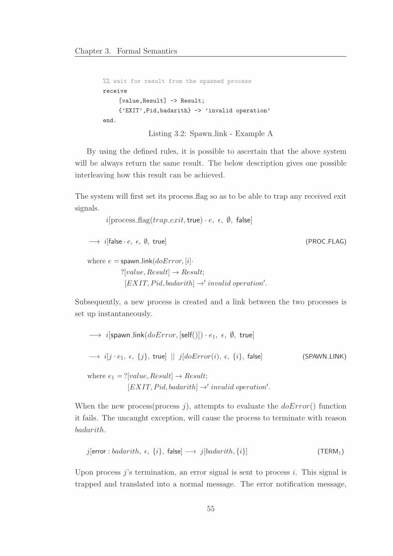
Chapter 3. Formal Semantics
%% wait for result from the spawned process
receive
[value,Result] -> Result;
{’EXIT’,Pid,badarith} -> ’invalid operation’
end.
Listing 3.2: Spawn link - Example A
By using the defined rules, it is possible to ascertain that the above system
will be always return the same result. The below description gives one possible
interleaving how this result can be achieved.
The system will first set its process flag so as to be able to trap any received exit
signals.
i[process flag(trap exit, true) · e, ε, ∅, false]
−→ i[false · e, ε, ∅, true] (PROC FLAG)
where e = spawn link(doError, [i]·
?[value,Result] → Result;
[EXIT, P id, badarith] →′ invalid operation′.
Subsequently, a new process is created and a link between the two processes is
set up instantaneously.
−→ i[spawn link(doError, [self()]) · e1, ε, ∅, true]
−→ i[j · e1, ε, {j}, true] || j[doError(i), ε, {i}, false] (SPAWN LINK)
where e1 =?[value,Result] → Result;
[EXIT, P id, badarith] →′ invalid operation′.
When the new process(process j), attempts to evaluate the doError() function
it fails. The uncaught exception, will cause the process to terminate with reason
badarith.
j[error : badarith, ε, {i}, false] −→ j[badarith, {i}] (TERM1)
Upon process j’s termination, an error signal is sent to process i. This signal is
trapped and translated into a normal message. The error notification message,
55

Chapter 3. Formal Semantics
[EXIT, j, badarith] is appended to process i’s mailbox.
−→ j[badarith, {i}] || i[e1, ε, {i}, true]
−→ j[badarith, ∅] || i[e1, [[EXIT, j, badarith]], ∅, true] (EXIT2)
The trapped error signal will be read, and the atom ‘invalid operation’ will be
returned.
≡ i[e1, [[EXIT, j, badarith]], ∅, true] || j[badarith, ∅]
−→ i[′invalid operation′, ε, {j}, true] || j[badarith, ∅] (RCV)
Now let’s consider the same system, but replacing spawn link by spawn followed
by a link as follows:
%% this function will cause the process to terminate
%% with reason badarith
doError(Pid) -> Pid ! a + a.
processA() ->
process_flag(trap_exit,true),
%% create new process
Pid = spawn(moduleName,doError,[self()]),
%% link to new process
link(Pid),
receive
[value,Result] -> Result
{EXIT,Pid,badarith} -> ’invalid operation’
end.
Listing 3.3: Spawn link - Example B
Even though the above system may still evaluate down to ’invalid operation’
it is also possible that the system returns a different result. This may occur if
the following sequence of steps occurs.
The system sets its process flag and creates the new process.
i[process flag(trap exit, true) · spawn(doError, [i]) · link(j) · e, ε, ∅, false]
56

Chapter 3. Formal Semantics
−→ i[false · spawn(doError, [i]) · link(j) · e, ε, ∅, true] (PROC FLAG)
−→ i[spawn(doError, [i]) · link(j) · e, ε, ∅, true] (SEQ1)
−→ i[j · link(j) · e, ε, ∅, true] || j[doError([i]), ε, ∅, false] (SPAWN)
where e =?[value,Result] → Result;
[EXIT, P id, badarith] →′ invalid operation′.
Process j will then attempt to evaluate doError and it fails. As a result, process
j terminates. Note however, that since there are no pids in its link set no error
signals will be sent.
j[error : badarith, ε, ∅, false] −→ j[badarith, ∅] (TERM1)
Subsequently, process i will attempt to link to process j. Since process j has
terminated it receives an error signal with reason noproc.
−→ i[link(j) · e, ε, ∅, true] || j[badarith, ∅] (TERM1)
−→ i[true, q ++ [′EXIT ′, j, noproc], ∅, true] || j[badarith, ε] (LINK1)
Due to the fact that the receive construct is only able to read exit message with
reason badarith, process j will then block indefinitely since no messages in its
mailbox pattern match against the provided patterns .
This really simple example illustrates that by calling a spawn followed by a
link, the system may sometimes evaluate to unwanted results. Perhaps this is one
of the main reasons why as mentioned in [17], the link call is rarely used in actual
Erlang systems. In fact, Erlang developers more often than not, opt to use solely
the spawn link function since this guarantees that the link is always carried out
instantly, ensuring that no error signals are lost.
57

Chapter 3. Formal Semantics
3.11.4 Explicit error signals
i 6= j ∧ v = killEXIT3
i[exit(j, v), mi, li, fi ] || j[ej , mj , lj , fj ] −→
i[true, mi, li, fi ] || j[killed, lj ]
i 6= j ∧ v 6= kill ∧ v 6= normal ∧ fj = falseEXIT4
i[exit(j, v), mi, li, fi ] || j[ej , mj , lj , fj ] −→
i[true, mi, li, fi ] || j[v, lj ]
i 6= j ∧ v = normal ∧ fj = falseEXIT5
i[exit(j, v), mi, li, fi ] || j[ej , mj , lj , fj ] −→
i[true, mi, li, fi ] || j[ej , mj , lj , fj ]
i 6= j ∧ v 6= kill ∧ fj = trueEXIT6
i[exit(j, v), mi, li, fi ] || j[ej , mj , lj , fj ] −→
i[true, mi, li, fi ] || j[ej , mj ++ [EXIT, i, v], lj , fj ]
EXIT7
i[exit(j, v), mi, li, fi ] || j[v, lj ] −→ i[true, mi, li, fi ] || j[v, lj ]
Table 3.11: Explicit exit signals
i = j ∧ v = killEXIT8
i[exit(j, v),m, l, f ] −→ i[killed, l]
i = j ∧ v 6= kill ∧ f = falseEXIT9
i[exit(j, v),m, l, f ] −→ i[v, l]
i = j ∧ v 6= kill ∧ f = trueEXIT10
i[exit(j, v),m, l, f ] −→ i[true,m++ [EXIT, i, v], l, f ]
Table 3.12: Self-sent exit signals
The above rules state how processes behave on receipt of an error signal which is
explicitly sent by another process. The diagram shown hereafter illustrates how
these rules relate to the behaviour of actual Erlang.
58

Chapter 3. Formal Semantics
Figure 3.3: Exit propagation through explicit error signals
In the above diagram Process A is the process which is generating the explicit
error signal by calling the exit(pid,Reason) built-in function. Here note, that
process A is calling the exit function twice i.e. exit(B,Reason), exit(C,Reason).
The key difference between process B and process C, is that process C is a system
process(process flag is set) while process B is not.
Perhaps the most noticeable difference between explicitly generated error sig-
nals and error propagation through links is when the reason of the generated
signal is kill. In this case, as stated in rule EXIT3, the receiving process will
terminate immediately with reason killed irrespective of whether it is trapping
exit signals or not. Rules EXIT4 and EXIT5 describe the way the system behaves
whenever an exit signal is sent to a process which is not trapping exit signals.
Rule EXIT4 states that when an exit signal with reason R(where R 6= to kill
or normal) is sent to a process which is not trapping exit signals, the receiving
59

Chapter 3. Formal Semantics
process will terminate with reason R. Otherwise, if an exit signal with reason
normal is sent to a process which is not trapping exit signals then this process
will not terminate(EXIT5). Rule EXIT6 states that when an exit signal is sent to
a process which is trapping exit signal, then the received signal is translated into
an exit message and appended to the process’ mailbox. Rule EXIT7 states that
if an exit signal is sent to a terminated process, then the exit signal is ignored.
Given the high degree of similarity between explicitly generated error signals
and error propagation through links, at this point it is worth considering if it
is possible to imitate the behaviour of links by sending explicit error signals.
For example, can the following two pieces of code be considered as semantically
equivalent?
Process i:
link(j),
link(k),
...
exit(badarg),
?⇔
Process i :
exit(j,badarg),
exit(k,badarg),
exit(badarg),
Listing 3.4: Exit propagation & Explicitly sent exit signals
At first glance, they seem to have identical behaviour - in both cases an exit
signal with reason badarg will be sent to process j and process k. However, there
is one subtle difference. In the first case process i will terminate prior to sending
any error signals whereas in the second case process j will send all error signals
before its termination. In order to better understand the consequence of such a
slight difference let’s consider the case where an external process, say process l
sends an exit signal with reason stop just after process i has sent an error signal
to process j.
First we will consider the piece of code shown on the left hand side. In this
case after linking to process j and process k, process i will terminate with reason
badarg.
i[link(j)·link(k)·...exit(badarg), ε, ∅, false] || j[ej, ε, ∅, false] || k[ek, ε, ∅, false]
−→ i[link(k) · exit(badarg), ε, {j}, false] || j[ej , ε, {j}, false] || k[ek, ε, ∅, false]
(LINK0)
60

Chapter 3. Formal Semantics
−→ i[exit(badarg), ε, {j, k}, false] || j[ej , ε, {j}, false] || k[ek, ε, {k}, false]
(LINK0)
−→ i[badarg, {j, k}] || j[ej , ε, {j}, false] || k[ek, ε, {k}, false] (TERM1)
After its termination, process i will start sending error signals to all processes
found in its link set; i.e. process j and process k. Here it is worth pointing
out that process i may first send an error signal to either process j or k since
as mentioned in Section 3.11.2 the order in which error signals are sent upon
process termination is undetermined. In the following steps process i will first
send an error signal to process j. Since process j is not trapping exit signals it
will terminate with reason badarg.
i[badarg, {j, k}] || j[e, ε, {i}, false] −→ i[badarg, {k}] || j[badarg, ∅] (EXIT2)
After the error signal has been sent, another different process l, sends an error
signal with reason stop to process i. Since process i has already terminated this
error signal will be ignored.
l[stop, {i}] || i[badarg, {k}] −→ l[stop, ∅] || i[badarg, {k}] (EXIT7)
Process i, will then continue sending error signals to the remaining processes
found in its link set i.e. process k. On receipt of the error signal process k will
also terminate with reason badarg.
i[badarg, {k}] || k[e, ε, {i}, false] −→ i[badarg, ∅] || k[badarg, {i}] (EXIT2)
Now let’s consider the scenario where no links are used. In this case process i will
first send an error signal to process j and just as before process j will terminate
with reason badarg.
i[exit(j, badarg), ε, ∅, false]|| j[e, ε, {i}, false] −→
i[true, ε, ∅, false] || j[badarg, ∅] (EXIT4)
Then process i will receive the error signal from process l. Since process i is not
trapping exit signals, this will cause process i to terminate immediately.
61

Chapter 3. Formal Semantics
l[stop, {i}] || i[true, ε, ∅, false] −→ l[stop, ∅] || i[stop, ∅] (EXIT2)
As a result process i would never be able to send the remaining error signal
to process k. This which may potentially result in a memory leak, if for instance
process k is blocked waiting for some message from process i. This particular
example proves that the behaviour of error propagation through links cannot
always be imitated by using explicit error signals.
Another major difference between links and explicit error signals is that an
explicit error signal can be sent to the process generating the signal itself. This
is done if the first argument of the exit built-in functions is set to the calling
process pid, exit(self(), Reason). In the case of links this behaviour cannot be
obtained, a process cannot be linked to oneself. The rules defining the behaviour
of processes when exit signals are sent to oneself are described in Table 3.11.4.
What these rules essentially state is that when sending error signals to oneselfthe behaviour of the process will depend mainly on two factors:
• the reason describing the cause of the error signal
• the process’s process flag
If the reason of the error signal is equal to kill, the process will die irrespective
of whether it is trapping exit signals or not(EXIT8). Otherwise, if the process is
trapping exit signals, the generated error signal will be trapped and a message
is appended to the process’ mailbox(EXIT10). If the process is not trapping exit
signals, the process will terminate immediately with the reason being the one set
by the explicitly generated error signal(EXIT9). Here it is worth highlighting the
fact that the process will still terminate even if the reason is set to normal.
In fact this is one minor improvement over Fredlund’s semantic definition of
explicitly generated error signals[14]. In his work, Fredlund does not define rules
to describe the behaviour of processes when error signals are sent to oneself. Con-
sequently, when trying to evaluate exit(self(),Reason) it is impossible to see how
the system will behave. For instance, let’s consider the case when the expression
exit(self(),normal) is evaluated. At first one might think that when evaluating
this expression the process will not terminate. This is because non-system pro-
cesses will only terminate upon receipt of an abnormal error signal (i.e. reason
6= normal). However, in truth when evaluating this expression using actual
Erlang the system will terminate immediately with reason normal.
62

Chapter 3. Formal Semantics
One problem mentioned in the previous chapter with respect to self-sent error
signals was if the function call exit(Reason) can be considered to be semantically
equivalent to exit(self(), Reason). Through the above semantics it becomes ev-
ident that there are some major difference between the two. For instance, let’s
consider the following two code excerpts:
process_flag(trap_exit,true),
....
exit(reason),
?⇔
process_flag(trap_exit,true),
....
exit(self(),reason),
Listing 3.5: exit(Reason) & exit(self(),Reason) - Case A
When trying to evaluate the code excerpt found on the left using the defined
semantics the exit(reason) will be first reduced to an exception. This exception
will then cause the process to terminate with reason reason.
i[exit : reason, ε, ∅, true] −→ i[reason, ∅] (TERM1)
If we attempt to evaluate the code excerpt found on the right hand side the
end process will be different. This is due to the fact that the exit(self(), reason)
will not cause the process to terminate. Instead an error signal notification is
added to its mailbox.
i[exit(self(), reason), ε, ∅, true] −→
i[true, [EXIT, i, reason], ∅, true] (EXIT10)
This scenario shows that the exit(Reason) function cannot be considered to be
semantically equivalent to exit(self(),Reason). Nonetheless, the above case only
illustrates that these two expressions are not equivalent when called from within
a system process. What if the process flag is set to false just before calling the
exit(self(), Reason)? In this case will the two expressions always behave in the
same way? In order to be able to tackle this problem let’s consider the following
code excerpts:
try
process_flag(trap_exit,false),
exit(reason),
catch
exit:reason -> caught
end
?⇔
try
process_flag(trap_exit,false),
exit(self(),reason),
catch
exit:reason -> caught
end
Listing 3.6: exit(Reason) & exit(self(),Reason) - Case B
63

Chapter 3. Formal Semantics
Using the defined semantics, the exit(reason) will be first reduced to an exception.
Since this is found within a try-catch block the generated exception will not cause
the process to terminate. As a result, the process will not terminate.
i[try exit : reason catch exit : reason → caught end, ε, ∅, false] −→
i[caught, ε, ∅, false] (TRY2)
In the second case, the exit(self(),reason) expression will send an exit signal to
itself. Due to the fact that the try-catch block is only capable of catching excep-
tions, the sent exit signal will immediately cause the process to terminate.
i[exit(self(), reason), ε, ∅, false] −→ i[reason, ∅] (EXIT9)
Therefore, even though at first it might seem that exit(self(), Reason) and
exit(Reason) will always behave in the same way when used by a non-system
process, this case proves that in truth this may not always be the case.
3.11.5 Monitors
MON0
i[monitor(process, j), mi, li, fi ]||j[ej, mj, lj, fj ] −→
i[true, mi, li, true ] || j[ej, mj, lj ∪ {i}, fj ]
MON1
i[monitor(process, j), m, l, f ] || j[v, l] −→
i[true, m++ {′EXIT ′, j, down}, l, f ] || j[v, l]
These rules state that when a process calls the monitor function, a one directional
link is created between the calling process and the specified pid(MON0). If the
process specified by the pid terminates abnormally, a notification message about
its termination will be sent. When the calling process, attempts to monitor
a terminated process, a notification message is immediately sent to the calling
process(MON1).
One point worth mentioning here is that these rules have two main limitia-
tions:
• In actual Erlang, when a process calls the monitor function consecutivetimes, multiple monitors are created. For instance, in the following example
64

Chapter 3. Formal Semantics
monitor(process, Pid1),
monitor(process, Pid1)
two monitors will be created. As a result when the process terminates, two
message notifications will be received. In our semantics, only one message
will be received since the link set will only contain one instance of the
monitor’s pid. (due to the fact that sets are not able to store duplicates)
• In actual Erlang, when a process calls the monitor function it will onlybe able to trap error signals from the process which it is monitoring. Forinstance, in the case shown hereafter:
monitor(process, Pid1),
link(Pid2)
the calling process is only able of trapping error signals from Pid1. If pro-
cess Pid2 fails abnormally, than the calling process will also fail. However,
by using the defined rules, it is not possible to faithfully describe this be-
haviour. In fact the defined rules assume that there will only be monitor
calls within one process.
Using the defined rules, we are now able to tackle another problem mentioned
in the previous chapter - Can the monitor behaviour be implemented using links
as illustrated in the following diagram?
Figure 3.4: Monitor and Links
The following two code excerpts, illustrate how the above two systems are imple-
mented in Erlang.
65

Chapter 3. Formal Semantics
Process i
monitor(process,Pid2),
....
%%error occurs - reason = stop
Process j
...
Process i
process_flag(trap_exit,true),
link(PidB),
...
%%error occurs - reason = stop
Process j
process_flag(trap_exit,true),
...
Listing 3.7: Monitors & Links
The two systems seem to be semantically equivalent. In both cases if process
j fails, process i will be notified through an error messages. Additionally, a failure
in process i should never cause process j to terminate since:
• in the case of monitors, an error signal will not be sent given that process
j is not included in process i’s links set.
• in the case of links, process j should be able to trap the received exit signal.
Nonetheless, by using the defined rules it is possible to see that this last
statement is not entirely true since in reality when using links, process j may
actually fail to trap the received exit signal. This occurs, if the following sequence
of reductions take place.
After setting its process flag, process i creates a link to process j.
i[link(j) · exit(stop), ε, ∅, true] || j[e, ε, {i}, false]
−→ i[true · exit(stop), ε, {j}, true] || j[e, ε, {i}, false] (LINK0)
where e = process flag(trap exit, true) · ...
Process i, then terminates abnormally with reason stop. Upon termination it
sends an error signal to process j. Since process j has not set its process flag yet,
the sent error signal will cause it to terminate immediately.
−→ i[stop, {j}] || j[e, ε, {i}, true] (TERM1)
66

Chapter 3. Formal Semantics
−→ i[stop, ∅] || j[stop, ∅] (EXIT2)
Therefore, this proves that even though at first it might seem that the two
code excerpts are equivalent in actual fact they are not. Here one can appreciate
the fact, that thanks to the defined rules it was possible to clearly identify the
subtle difference between the two mechanisms.
3.11.6 sumNProduct Example(Remote error handling)
Using this rule it is now possible to describe the behaviour of sumNProduct which
makes use of the remote handling mechanisms as described in 3.11.2. Here, it
is important to note that in the following descriptions only the main reduction
steps are described. This is due to the fact that if all the reduction steps were to
be mentioned, the system’s description may result in a rather lengthy one.
First, we will consider the case when the both input lists consists are set to
[12,5]. First the parent process sets its flag so that it will be able to trap any
received error signals.
i[process flag(trap exit, true) · e1, ε, ∅, false]
−→ i[false · e1, ε, ∅, true] (PROC FLAG)
where e1 = spawn link(sumProcess, [i, [12, 5]]) · spawn link(productProcess, [i, [12, 5]])·
?[sum, Sum] → Sum; [EXIT, j, badarith] → invalid·
?[product, Product] → Product; [EXIT, k, badarith] → invalid·
[Sum,Product]
Two seperate processes are then created. Since the spawn link function is used a
link between the child and parent process is set up immediately. First the process
which is responsible to compute the sum is spawned:
−→ i[spawn link(sumProcess, [i, [12, 5]]) · e2, ε, ∅, true] (SEQ1)
−→ i[j · e2, ε, {j}, true] || j[i![sum, 12 + 5]), ε, {i}, false] (SPAWN LINK)
67

Chapter 3. Formal Semantics
where e2 = spawn link(productProcess, [i, [12, 5]])·
?[sum, Sum] → Sum; [EXIT, j, badarith] → invalid·
?[product, Product] → Product; [EXIT, k, badarith] → invalid·
[Sum,Product]
Subsequently, another process is spawned to calculate the product of the input
list.
−→ i[spawn link(productProcess, [i, [12, 5]]) · e3, ε, {j}, true] ||
k[i![product, 12 ∗ 5], ε, {i}, false] || sj (SEQ1)
−→ i[k · e3, ε, {k}, true] || k[i![product, 12 ∗ 5], ε, {i}, false] || sj (SPAWN LINK)
−→ i[e3, ε, {j, k}, true] || k[i![product, 12 ∗ 5], ε, {i}, false] || sj (SEQ1)
where sj = j[i![sum, 12 + 5]), ε, {i}, false]
e3 =?[sum, Sum] → Sum; [EXIT, j, badarith] → invalid·
?[product, Product] → Product; [EXIT, k, badarith] → invalid·
[Sum,Product]
Process j, the process calculating the sum will then send its result.
≡ j[i![sum, 12 + 5]), ε, {i}, false] || i[e3, ε, {j, k}, true] || s′k
−→ j[[sum, 17], ε, {i}, false] || i[e3, [[sum, 17]], {j, k}, true] || s′k (SEND1)
Subsequently process k will send the the product of the input list.
≡ k[i ! [product, 60], ε, {i}, false] || i[e3, ε, {j, k}, true] || s′j
−→ k[[product, 17], ε, {i}, false] ||i[e3, [[sum, 17], [product, 60]], {j, k}, true] || s′j
(SEND1)
where s′k = k[i![product, 12 ∗ 5]), ε, {i}, false]
s′j = j[[sum, 17], ε, {i}, false]
The two results are then read from the mailbox. First process i will read the sum
value.
68

Chapter 3. Formal Semantics
≡ i[?[sum, Sum] → Sum; [EXIT, j, badarith] → invalid · e4,
[[sum, 17], [product, 60]], {j, k}, true] || s′′j || s′′k
−→ i[17 · e4, [[product, 60]], {j, k}, true] || s′′j || s′′k (RCV)
where e4 = ?[product, V alue] → V alue; [EXIT, k, badarith] → invalid
·[17, P roduct]
s′′k = k[[product, 60], ε, {i}, false]
s′′j = j[[sum, 17], ε, {i}, false]
Then process i will then read the product value. The two read values i.e. [17,60]
are then returned.
−→ i[?[product, Product] → Product; [EXIT, k, badarith] → invalid
·[17, P roduct], [[product, 60]], {j, k}, true] || s′′j || s′′k
−→ i[[17, 60], ε, {j, k}, true] || s′′j || s′′k (RCV)
The above reduction steps are only one possible sequence of steps that can
lead to the expected output. As mentioned in a previous section, when dealing
with a parallel system there may be various different interleavings which still lead
to the same output. Nonetheless, through the defined rules it is possible to check
that all possible interleavings lead to the same result.
We will now consider the case when invalid list of data is input - [a,12]. Note
that here only the main reduction steps are highlighted. These will give an idea
how the defined rules can be used to describe the behaviour of a system. Similar
to the previous case, process i will first set its process flag.
i[process flag(trap exit, true) · e1, ε, ∅, false]
−→ i[false · e1, ε, ∅, true] (PROC FLAG)
where e1 = spawn link(sumProcess, [i, [a, 12]]) · spawn link(productProcess, [i, [a, 12]])·
?[sum, Sum] → Sum; [EXIT, j, badarith] → invalid·
?[product, Product] → Product; [EXIT, k, badarith] → invalid·
[Sum,Product]
Then it will spawn the two processes, one to calculate the sum and another to
calculate the product.
69

Chapter 3. Formal Semantics
−→ i[spawn link(sumProcess, [i, [a, 12]]) · e2, ε, ∅, true] (SEQ1)
−→ i[j · e2, ε, {j}, true] || j[i![sum, a+ 12]), ε, {i}, false] (SPAWN LINK)
where e2 = spawn link(productProcess, [i, [a, 12]])·
?[sum, Sum] → Sum; [EXIT, j, badarith] → invalid·
?[product, Product] → Product; [EXIT, k, badarith] → invalid·
[Sum,Product]
Subsequently, another process is spawned to calculate the product of the input
list.
−→ i[spawn link(productProcess, [i, [a, 12]]) · e3, ε, {j, k}, true] ||
k[i![product, a ∗ 12], ε, {i}, false] || sj (SEQ1)
−→ i[k · e3, ε, {j, k}, true] || k[i![product, a ∗ 12], ε, {i}, false] || sj (SPAWN LINK)
−→ i[e3, ε, {j, k}, true] || k[i![product, a ∗ 12], ε, {i}, false] || sj (SEQ1)
where sj = j[i![sum, a+ 12]), ε, {i}, false]
e3 =?[sum, Sum] → Sum; [EXIT, j, badarith] → invalid·
?[product, Product] → Product; [EXIT, k, badarith] → invalid·
[Sum,Product]
When processes j attempts to calculate the sum of the received list it will fail
with reason badarith. Afterwards, it will send an error signal to process i.
≡ j[i![sum, a+ 12]), ε, {i}, false] || i[e3, ε, {j, k}, true] || s′k
−→ j[error : badarith, ε, {i}, false] || i[e3, ε, {j, k}, true] || s′
k
−→ j[badarith, i] || i[e3, ε, {j, k}, true] || s′
k (TERM1)
−→ j[badarith, ∅] || i[e3, [[EXIT, j, badarith]], {k}, true] || s′k (EXIT2)
where s′k = k[i![product, a ∗ 12]), ε, {i}, false]
Process i will then read the received error notification
70

Chapter 3. Formal Semantics
≡ i[?[sum, Sum] → Sum; [EXIT, j, badarith] → invalid · e4,
[[EXIT, j, badarith]], {k}, true] || j[badarith, ∅] || s′k
−→ i[invalid · e4, ε, {k}, true] || j[badarith, ∅] || s′k (RCV)
where e4 =?[product, V alue] → V alue; [EXIT, k, badarith] → invalid
·[invalid, Product]
Similarly, process k will also terminate with reason badarith. The received error
notification will be appended to process i’s mailbox.
≡ k[i![product, 12 ∗ 5], ε, {i}, false] || i[invalid · e4, ε, {k}, true] || s′j
−→ k[error:badarith, ε, {i}, false] || i[invalid · e4, ε, {k}, true] || s′j
−→ k[badarith, {i}] || i[invalid · e4, ε, {k}, true] || s′j (TERM1)
−→ k[badarith, ∅] || i[e4, [[EXIT, k, badarith]], ∅, true] || s′j (EXIT2)
where s′j = j[badarith, ∅]
Process i will read the error notification sent from process k.
−→ i[?[product, Product] → Product; [EXIT, k, badarith] → invalid·[invalid, Product],
[[EXIT, k, badarith]], ∅, true] || s′k || s′j
−→ i[[invalid, invalid], ε, ∅, true] || s′k || s′j (RCV)
where s′k = k[badarith, ∅]
The above steps show that in the case of invalid input, this version of sumN-
Product will also return [invalid, invalid] just like its sequential and other parallel
version. By using the defined rules it is also possible to show that even by chang-
ing the order in which the events happen the system will still return the same
output if given the same input. Therefore, it is possible to conclude that this
version of sumNProduct is semantically equivalent to its previous versions.
71
Chapter 3. Formal Semantics
3.12 Conclusion
This chapter presented a formal semantic definition of Erlang’s error handling
mechanisms. These formal definitions provided us a better insight of how Er-
lang systems behave in the presence of errors. In fact, by using these rules it
became possible to get a step-by-step description of how Erlang systems are ex-
ecuted, bringing to light any unexpected sequences of events that may lead to
unwanted results. Additionally, these rules were also able to show that in some
cases, two syntactically different systems can actually have semantically equiva-
lent behaviour. However, when dealing with parallel system it was much more
challenging to ensure semantic equivalence of two systems. This is due to the fact
that the number of possible interleavings is exponential to the size of the given
system. This latter fact, is the motivation behind the next chapter. In order
to facilitate the task of exhaustively analysing a system’s behaviour, the defined
semantic rules will be animated through an evaluator.
72

4. Implementation Framework
4.1 Introduction
The main motivation behind defining a formal semantics for the error handling
constructs was to be able to correctly reason about Erlang systems. Through
the rules defined in the previous chapter it became possible to give a detailed
description of how a particular Erlang system is expected to behave. The aim of
this chapter is to give a high-level description of the system which was designed so
as to be able to check the behaviour of a system under all possible interleavings
in a more efficient way. The main components of the designed system will be
outlined highlighting any choices that were taken whilst designing the system.
4.2 System Design
The system was implemented in Haskell and as illustrated in Figure 4.1, it consists
mainly of three main modules. The first module is responsible for parsing the
input text. The parsed input is then fed to the evaluator which will describe all
possible ways the input system may behave according to the previously defined
semantic rules. The last module’s task is to present in an understandable way, a
step-by-by description of these different behaviours. In the following sections we
will take a deeper look at hwoeach of these modules.
73

Chapter 4. Implementation Framework
Figure 4.1: System’s design
4.3 Input
The designed system asks the user to enter three inputs:
1. name of the module file - The module file should contain the function defi-
nitions that are called by the Erlang system. Even though in actual Erlang
one system can call functions, whose definitions are found within different
modules in the designed system, all function definitions have to be found
within the same file. The expressions of this file will be parsed according
to the BNF described in Table 3.2. The only difference is that the spawn,
spawn link, and spawn monitor functions do not expect the module name
parameter.
2. name of the input file - this file will contain the input expression that in
actual Erlang is input into the shell. This expression will be also parsed
according to the BNF described in Table 3.2 and as in the previous case the
spawn, spawn link and spawn monitor functions do not expect the module
name parameter.
3. name of the output file - this will determine the name of the file where the
results of the evaluator will be stored.
4.4 Parsing
The first module is composed of two distinct sub-modules; the lexer and the
parser. The purpose why the parsing analysis was divided into two stages is that
this approach helps in ensuring a less complex design for the parser.
74

Chapter 4. Implementation Framework
4.4.1 Lexer
The lexer used within the system was adapted from the one found in [20]. As
input the lexer will be fed text upon which it performs the following taks:
- remove comments
- remove white spaces
- detect any lexical errors
- recognise any keywords or operators
- recognise atoms and integers
For example, if the lexer is given the following input:
%% this is an example
[1,20,Hello,world]
it will tokenize the input text and return the following list of tokens.
[Tok "[" 3 2 Keyword,
Tok "1" 3 3 Number,
Tok "," 3 4 Keyword,
Tok "10" 3 5 Number,
Tok "," 3 7 Keyword,
Tok "Hello" 3 8 Variable,
Tok "," 3 13 Keyword,
Tok "world" 3 14 UnquotedAtom,
Tok "]" 3 19 Keyword,
Tok "" 3 20 EndToken]
Each token has a string containing the exact substring from the source file
followed by the line and column where the token is found in source file and the
token’s class such as Number or Variable. This tokenized list is then passed to
the parser.
4.4.2 Parser Combinators
The parser was implemented using parser combinators rather than a parser gener-
ator. One major benefit of using parser combinators is that one need not generate
the whole parser every time a minor modification is done to the parser as is the
case when using a parser generator. The fundamental principle behind parser
combinators is that a parser is written in bottom-up fashion, similar to the way
that one would define a language grammar.
75

Chapter 4. Implementation Framework
In fact, when implementing the parser for this project the most elementary
parser were first defined. These parsers were then “joined” together so as to get
the main parser which is able to parse all of the expressions found in the chosen
subset of Erlang. The most basic parser within the designed system is the token
parser.
token ([]) = ParseError "Unexpected eof"
token (x:xs) = Expression (x,xs)
Listing 4.1: Basic Parser
The task of this simple parser is to return as the parsed expression, the head
of the token’s list that is passed to the main parser. Apart from the token
parser, several other elementary parsers were defined. These all combined the
token parser described above with another function in order to produce a new
parser. One such parser is the keyword parser.
keyword str = token <=> (isKeyword str)
Listing 4.2: Keyword parser
Here, the <=> combinator, checks if the function given on the right hand side,
(isKeyword str), returns true when applied to the parsed expression that is
produced when using the parser on the left hand side (token). The keyword
parser was then combined to other elementary parsers which are needed to parse
the Erlang expressions that are found in the chosen subset. Two such expression
parsers are the following:
caseExp = (keyword "case") <-+>
expression <+->
(keyword "of") <+>
erlangMatch
tryExp = (keyword "try") <-+>
sequence <+->
(keyword "catch") <+>
exceptionsCatch
Listing 4.3: Parser Combinators
These parsers make use of three different parser combinators. The <+> com-
binator joins two parsers using the ‘and’ type operator. The <-+> combinator is
similar to the <+> combinator but does not return the output of the parser on the
left hand side of the combinator. On the other hand, the <+-> combinator does
not return the output of the parser defined on the right hand side. For instance,
76

Chapter 4. Implementation Framework
when applying the caseExp parser to a tokenized list representing the following
expressions:
case Value of 1 -> hello; 2 -> bye end
try A+B catch error:Desc -> Desc end
the Erlang expression parser returns the expression
Case (Var "Value") Match [(1,Atom "hello"),(2,(Atom "bye")]
Try (Add (Var A) (Var B)) Match [Exception Error (Var Desc)]
In order to be able to parse all the expressions in the subset, a different
simple parser were defined for each Erlang expression. Here, only the tryExp
and caseExp parsers were described. However, the other parsers were defined
similar to the way in which these two parsers have been defined.
The main parser then “combined” all of these expression parser by using the
<|> combinator whose task is to join any two elementary parsers using the ‘or’
type operator.
prefixExp :: Parser ErlangExp
prefixExp =
caseExp
<|> receiveExp
<|> tryExp
<|> builtInFun
<|> functionCall
<|> list
<|> atom
<|> number
<|> var
Listing 4.4: Expressions Parser
The above parser is used to parse the Erlang expressions found in the chosen
subset. Once again, through this example one cannot help noticing the fact
parser combinators made it possible to define the parser using really neat syntax.
Moreover the parser’s syntax is highly similar to the BNF definition. In fact,
by looking at the parser definitions in 4.4 one can immediately understand what
expression a particular parser is expected to parse since the parser function is
almost identical to the BNF definition.
77

Chapter 4. Implementation Framework
Another reason why it was opted to implement the parser through parser
combinators lies in the fact that this approach allows incremental development.
Therefore, if for instance the parser were to be extended so as to be able to parse
Erlang tuples it would be relatively easy to carry out such modification. This
is because in order to extend the parser one need only define a simple parser to
parse Erlang tuples. The simple parser is then “joined” to the main parser as
described in Listing 4.5
prefixExp :: Parser ErlangExp
prefixExp =
caseExp
<|> receiveExp
<|> tryExp
<|> builtInFun
<|> functionCall
<|> list
<|> atom
<|> number
<|> var
<|> tuple
Listing 4.5: Expression Parser Extended
This simple example brings to light the fact that when using parser combi-
nators, no major modifications need to be done in order to increase the number
of expressions that the parser is able to parse. Therefore, with regards to this
work, even though the parser was defined for a subset of Erlang, it will be quite
straightforward to extend the parser so as to be able to accept an increased sub-
set of Erlang. In fact, if a parser were to be defined to accept a larger subset of
Erlang there will not be a need to implement the new parser from scratch as is
the case when parser generators are used. This is because the parser implemented
for this project may serve as the basis upon which the larger parser is built.
4.5 Evaluator
The primary aim of the evaluator is to give a clear and accurate description of
how a particular Erlang system behaves. This is done by going through all pos-
sible sequences of reduction steps that the system might take, possibly revealing
any unexpected ways in which an Erlang system might behave. Undoubtedly,
one of the major benefits of the designed evaluator is that it makes the task of
78

Chapter 4. Implementation Framework
checking the behaviour of a system under all possible interleavings much more
efficient. One here should be aware that the total number of interleavings can be
considerably large even when the input system is extremely simple. This can be
clearly seen if we consider the following really simple system:
processA() ->
%% create a new process send the value 3
case spawn_link(processB,[]) of
%% send the value 3 to the new process
Pid -> Pid ! 3
end.
processB() ->
%% bind the sum of 1+2 to Total
case 1+2 of Total ->
%% add the received Value to Total
receive
Value -> Total + Value
end
end.
Listing 4.6: Erlang Program
The following two lists identify all the small subtasks that are carried out by
each process when the system is executed. Each of these tasks corresponds to
exactly one reduction step.
Process A :
A1 : spawn new process
A2 : bind Pid to pid of new process
A3 : send message to process B
Process B :
B1 : compute sum of 1+2
B2 : bind Total to the result
B3 : receive message
B4 : add Total to the received Value
Table 4.1: Actions to be performed when executing program 4.6
Diagram 4.2 illustrates the different sequences of reduction steps that this
particular system may take before it returns its final output.
79

Chapter 4. Implementation Framework
Figure 4.2: Different interleavings
In the above diagram the actions that are done by process A are indicated
by gray coloured boxes, whereas actions that are carried out by process B are
indicated by white boxes.
One here may notice that in all cases, process A will send the message to
process B, and process B will always evaluate down to 6. Therefore, all cases
can be considered to have identical behaviour even though the sequence of steps
that led the system to achieve its final result are slightly different. Through this
diagram it becomes clear that one extra reduction step in any of the given process,
will increase the number of possible interleavings drastically.
In order to reduce the number of interleavings that the evaluator needs to
go through, it was decided that sequences of reduction steps that do not cause
any side effects, such as evaluation of addition followed by binding of variables
should be considered as one single operation. This is due to the fact, that the
order in which non-side effect reduction steps occurs may never yield to a different
system’s behaviour. For instance, let’s consider again the program described in
4.6. In this case, as described in 4.1 the majority of the actions that are carried
out by the two processes are non-side effect actions. In fact, the only side-effect
action is A3.
Therefore, it does not make any real difference if B1 is computed before A2,
or vice versa. This is because, non-side effect actions may only effect the local
state of the process. By adopting such a practice, the number of interleavings
is reduced substantially. This fact, is quite evident through Diagram 4.3 which
shows the reduced number of different interleavings that the evaluator will check
when using this approach.
80
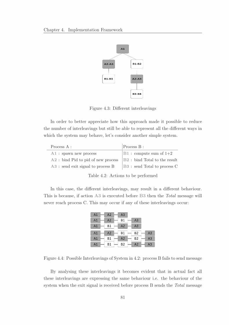
Chapter 4. Implementation Framework
Figure 4.3: Different interleavings
In order to better appreciate how this approach made it possible to reduce
the number of interleavings but still be able to represent all the different ways in
which the system may behave, let’s consider another simple system.
Process A :
A1 : spawn new process
A2 : bind Pid to pid of new process
A3 : send exit signal to process B
Process B :
B1 : compute sum of 1+2
B2 : bind Total to the result
B3 : send Total to process C
Table 4.2: Actions to be performed
In this case, the different interleavings, may result in a different behaviour.
This is because, if action A3 is executed before B3 then the Total message will
never reach process C. This may occur if any of these interleavings occur:
Figure 4.4: Possible Interleavings of System in 4.2: process B fails to send message
By analysing these interleavings it becomes evident that in actual fact all
these interleavings are expressing the same behaviour i.e. the behaviour of the
system when the exit signal is received before process B sends the Total message
81

Chapter 4. Implementation Framework
to process C. Here, it is worth highlighting the fact that in Erlang systems once a
process dies, all the information stored within local variables is lost. As a result,
with regards to this example, it does not really matter if the exit signal is received
after executing step B1 or just after executing B2. This is because, upon process
B’s termination all information stored in variables is lost.
Now, let’s consider the case when codeCommB3 is evaluated before A3 and
therefore the Total message will be successfully sent to process C. As in the
previous case, there are several possible different interleavings that may lead
process B to eventually send the Total message. These interleavings are described
in Figure 4.5.
Figure 4.5: Possible Interleavings of System in 4.2: process B sends message
Through this example it became evident that an Erlang system due to its
parallel nature may take different interleavings to complete its task. However,
the behaviour of a system is really determined by the order in which the side-
effect actions take place. For instance, with respect to this system, what really
matters is if the exit message is received before or after the Total message is
sent to process C. Therefore, all the different behaviours in which this particular
system may behave can be represented through the following two interleavings.
Figure 4.6: Possible Interleavings of System 4.2
Here, it is important to note that even though the number of interleavings to
be checked are reduced substantially, the different interleavings are still able to
represent all the possible ways in which a system may behave.
82

Chapter 4. Implementation Framework
One of the major benefits of reducing the number of possible interleavings was
that the evaluator experienced a slight improvement in efficiency. Just the same,
the number of possible interleavings in some cases is considerably large especially
when dealing with systems in which processes may terminate abnormally. This
is due the fact that the order in which exit signals are sent is undefined. For
instance, if a process is linked to 3 other processes, say process A, process B and
process C then there are a total of six different orderings in which the exit signal
may be sent. (since the failed process may send its exit signals either to A then
to B and then to C, or first to B, then to A and then to C ...) Let’s consider the
following example, to better understand how the order in which exit signals are
sent may increase significantly the number of possible interleavings:
...
%% spawn and link to process A
spawn_link(waitError,[Pid,ProcessB]),
%% spawn and link process B
spawn_link(waitError,[Pid,ProcessC]),
%% process terminates abnormally
%% with reason ’error occured’
exit(’error occured’).
waitError(Pid,Name) ->
%% start trapping exit signals
process_flag(trap_exit,true),
%% wait for error message
receive
Error -> Pid ! Name
end.
Listing 4.9: Erlang Program using Remote Error Handling Mechanisms
Each process in the above system, needs to execute the following steps:
Process A :
A1 : spawn link process B
A1 : spawn link process C
A3b : send error signal to B
A3c : send error signal to C
Process B :
B1 : set process flag
B2 : receive error message and
send result to Pid
Process C :
C1 : set process flag
C2 : receive error message and
send result to Pid
Table 4.3: Actions to be performed when executing program 4.9
83

Chapter 4. Implementation Framework
In this case process A is linked to both process B and process C and therefore
it needs to send an exit signal to both processes. The evaluator needs to cover
both when A sends its exit signal first to process B and when process A sends its
exit signal first to process C. This factor, is one major contributor to the increase
in the number of sequences that need to be checked by the evaluator. To get a
better idea, how large this number can actually get, let’s consider the following
diagram which describes the different interleavings that the system described
above may take:
Figure 4.7: Error handling - possible interleavings
Given the fact, that the number of different sequences may become consid-
erably large, it was decided that in the final output the evaluator only includes
the different end result the system might reach and one sequence that may lead
to this end result. For instance, in the above system, since the system may end
in five different ways in the output file only five sequence of reductions steps are
included, even though there are more different interleavings that the system may
take.
4.6 Building the Output File
Once the evaluator has gone through all the interleavings, an output file is built
decribing the different ways in which the input system may behave. The output
file consists of a pdf file, which is composed primarily of four sections
84

Chapter 4. Implementation Framework
- function definitions
- shell input
- different end systems
- sequence of reduction steps that have led to the above end systems
In order to build the pdf file, the output of the evaluator is translated into a
latex file. This is then parsed by using the pdflatex command. Once the output
file has been built, the system will automatically open the file so that the user
may view the result of the evaluator.
4.7 Conclusion
This chapter gave a brief overview of the main components found within the
designed system. It also illustrated why parallel systems may go through several
different sequences of reduction steps before completing their task. As a result, it
became evident that when dealing with parallel systems the use of an evaluator
is key in order to identify those sequences of steps that may lead to unexpected
behaviour.
85

5. Evaluation
5.1 Introduction
The aim of this chapter is to measure to what degree the objectives set forth
in the beginning of this project have been met. These objectives were primarily
that the defined model should be able to:
- offer a better insight into Erlang’s error handling mechanisms
- explain better those circumstances that lead to unexpected results
- predict a system’s behaviour
- lay foundations for a semantic theory
In the first section of this chapter the evaluation strategy that is used is ex-
plained. Subsequently, the described evaluation strategy is applied to a number
of Erlang systems in order to evaluate to what extent the initial objectives have
been achieved. Finally, the results of the evaluation are discussed.
5.2 Evaluation Strategy
Since the semantics were defined post-hoc, it was important to ensure that the
presented definitions are loyal to the behaviour of actual Erlang. The correctness
of the defined model was measured by adopting the strategy described in Figure
5.1.
86

Chapter 5. Evaluation
Figure 5.1: Evaluation Strategy
The correctness of the model was analysed by considering a number of different
Erlang programs.
1. Each program was first run on the Erlang VM. In order to get a clearer
picture of how a program is evaluated, Erlang’s trace built-in function was
used. This function returns a step-by-step description of how a program has
been evaluated by Erlang, hence indicating the order in which side-effect
actions such as linking and delivery of exit signals took place.
2. The same Erlang program was then translated in terms of the model.
3. Subsequently, the translated Erlang program was input into the evaluator.
The evaluator returned sequences of reduction steps describing the different
ways the input program may be evaluated according to the defined model.
4. The output generated by Erlang’s tracer and the output of the evaluator are
compared to analyse if the defined rules are capable of faithfully describing
Erlang’s behaviour.
5.3 Assessing the Defined Model
In this section, the evaluation strategy is applied to several Erlang programs. The
programs were selected in such a way to evaluate all the rules which were defined
to describe Erlang’s error handling behaviour.
87
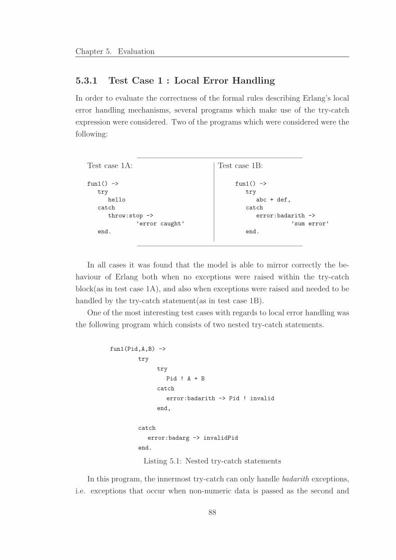
Chapter 5. Evaluation
5.3.1 Test Case 1 : Local Error Handling
In order to evaluate the correctness of the formal rules describing Erlang’s local
error handling mechanisms, several programs which make use of the try-catch
expression were considered. Two of the programs which were considered were the
following:
Test case 1A:
fun1() ->
try
hello
catch
throw:stop ->
’error caught’
end.
Test case 1B:
fun1() ->
try
abc + def,
catch
error:badarith ->
’sum error’
end.
In all cases it was found that the model is able to mirror correctly the be-
haviour of Erlang both when no exceptions were raised within the try-catch
block(as in test case 1A), and also when exceptions were raised and needed to be
handled by the try-catch statement(as in test case 1B).
One of the most interesting test cases with regards to local error handling was
the following program which consists of two nested try-catch statements.
fun1(Pid,A,B) ->
try
try
Pid ! A + B
catch
error:badarith -> Pid ! invalid
end,
catch
error:badarg -> invalidPid
end.
Listing 5.1: Nested try-catch statements
In this program, the innermost try-catch can only handle badarith exceptions,
i.e. exceptions that occur when non-numeric data is passed as the second and
88
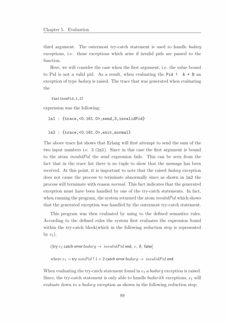
Chapter 5. Evaluation
third argument. The outermost try-catch statement is used to handle badarg
exceptions, i.e. those exceptions which arise if invalid pids are passed to the
function.
Here, we will consider the case when the first argument, i.e. the value bound
to Pid is not a valid pid. As a result, when evaluating the Pid ! A + B an
exception of type badarg is raised. The trace that was generated when evaluating
the
fun1(nonPid,1,2)
expression was the following:
ln1 : {trace,<0.161.0>,send,3,invalidPid}
ln2 : {trace,<0.161.0>,exit,normal}
The above trace list shows that Erlang will first attempt to send the sum of the
two input numbers i.e. 3 (ln1). Since in this case the first argument is bound
to the atom invalidPid the send expression fails. This can be seen from the
fact that in the trace list there is no tuple to show that the message has been
received. At this point, it is important to note that the raised badarg exception
does not cause the process to terminate abnormally since as shown in ln2 the
process will terminate with reason normal. This fact indicates that the generated
exception must have been handled by one of the try-catch statements. In fact,
when running the program, the system returned the atom invalidPid which shows
that the generated exception was handled by the outermost try-catch statement.
This program was then evaluated by using to the defined semantics rules.
According to the defined rules the system first evaluates the expression found
within the try-catch block(which in the following reduction step is represented
by e1).
i[try e1 catch error:badarg → invalidP id end, ε, ∅, false]
where e1 = try nonPid ! 1 + 2 catch error:badarg → invalidP id end
When evaluating the try-catch statement found in e1 a badarg exception is raised.
Since, the try-catch statement is only able to handle badarith exceptions, e1 will
evaluate down to a badarg exception as shown in the following reduction step:
89

Chapter 5. Evaluation
Evaluating subexpression e1:
i[try nonPid ! 1 + 2 catch error:badarith → Pid!invalid end, ε, ∅, false]
−→ i[error:badarg , ε, ∅, false]
The raised exception is then handled by the outermost try-catch statement and
the atom invalidP id is returned.
i[try error:badarg catch error:badarg → invalidP id end , ε, ∅, false]
−→ i[invalidP id , ε, ∅, false]
Subsequently, since there is no other expression to evaluate after the try-catch
statement the process terminates normally.
−→ i[normal, ∅]
The same behaviour was described when the program was input into the evalua-
tor:
Figure 5.2: Local error handling - evaluator’s output
As seen in Figure 5.2, the evaluator described the fact that the raised excep-
tion is handled by the outermost try-catch statement(TRY2). Subsequently, the
90

Chapter 5. Evaluation
process terminates with reason normal(TERM0).
With regards to the output generated by the evaluator, here it is important
to note that the expression in each reduction step only describes the innermost
evaluating expression. For instance, in the first reduction step, only the nonPid!3
expression found in process i is shown even though in actual fact this expression
is found within a try-catch statement. The main reason why it was opted to only
show the innermost evaluating expression was to prevent the reduction steps
descriptions from becoming too cumbersome.
Here, it is evident that the reduction steps describe a behaviour which is identical
to the one of actual Erlang. Therefore, it is clear that in this particular test case
the defined model is able to faithfully describe the behaviour of actual Erlang.
We will now move on to see if the behaviour of Erlang’s remote error handling
mechanisms as described by the model is completely faithful to the behaviour of
Erlang.
5.3.2 Test Case 2 : Remote Error Handling - Links
In Erlang whenever a process, say process A terminates with reason R then an
exit signal is sent to all of A’s linked processes. Upon receipt of this exit signal,
the linked process, say process B may behave in either of the following way:
case A: if process B’s process flag is set, an exit notification is appended to
process B’s mailbox
case B: if process B’s process flag is unset and R is normal, then the process
B ignores the received signal
case C: if process B’s process flag is unset and R is not equal to normal,
then the receiving process terminates with reason R
In order to check if the error propagation behaviour as described by the model
is correct, the test cases were chosen in such a way to cater for all the three
different ways a process might behave on receipt of an exit signal due to the
termination of a linked process. Here, only the evaluation of case A is described
since the evaluation carried out for each of the other cases is quite similar to the
one described here.
In the chosen program, one process is used to handle the generated exception
whereas another seperate process is responsible to compute the summation of the
91
Chapter 5. Evaluation
two input numbers.
fun1(Num1, Num2) ->
%% set process flag
process_flag(trap_exit,true),
%% create new process to compute sum of numbers
Pid = spawn_link(?MODULE,sum,[self(),Num1,Num2]),
receive
{’EXIT’,Pid,Error} -> invalid;
Result -> Result
end.
sum(Pid,Num1,Num2) -> Pid ! Num1 + Num2.
Listing 5.2: Remote Error Handling Example
When running this test case, the fun1() function was passed non-numeric data
(aa,bb) so as to see how the system will behave when incorrect data is input. The
generated trace list was as follows:
ln1 : {trace,<0.125.0>,spawn,<0.126.0>,{links,sum,[<0.125.0>,aa,bb]}}
ln2 : {trace,<0.125.0>,link,<0.126.0>}
ln3 : {trace,<0.126.0>,exit,{badarith,[{links,sum,3}]}}
ln4 : {trace,<0.125.0>,’receive’,{’EXIT’,<0.126.0>,
{badarith,[{links,sum,3}]}}}
ln5 : {trace,<0.125.0>,getting_unlinked,<0.126.0>}
ln6 : {trace,<0.125.0>,exit,normal}
In the above trace list, each side-effect action is represented by a tuple. The
second element of every tuple identifies the Pid of the process performing the
action. The third element gives the name of the side effect action that has been
done. In the case of spawning the fourth element shows the Pid of the new pro-
cess, whilst the fifth element shows the arguments passed to the spawn function
basically {moduleName, functionName, arguments}. In the case of linking, the
third element refers to the pid of the process with whom the link will be done.
92

Chapter 5. Evaluation
When the process terminates the third tuple is set to exit and the fourth tuple
indicates the reason with which the process terminated.
Here, one can appreciate how the trace list made it possible to get a really
clear picture of how this particular program is evaluated. In order to better
understand Erlang’s behaviour as described by the trace list let’s consider the
following diagram.
Figure 5.3: Remote error handling - Trace list’s output
The trace list describes the fact that the parent process (<0.125.0>) first
spawns and links to a new process(<0.126.0>)(ln1 - ln2). The task of the new
process is to compute the sum of aa and bb. Since the new process fails to com-
pute the sum of aa and bb it terminates with reason badarith(ln3). Once process
<0.126.0> terminates, an exit message is appended to process <0.125.0>’s mail-
box(ln4). The link which was found between the two processes is removed(ln5).
Subsequently, process <0.125.0> reads the exit message and terminates nor-
mally(ln6).
When the same system was input into the evaluator, the following sequence
of reductions was described. The parent process(process i), will first set its pro-
cess flag to true so as to trap any received exit signals.
93

Chapter 5. Evaluation
i[process flag(trap exit, true) · e1, ε, ∅, false]
−→ i[false · e1, ε, ∅, true]
where e1 = spawn link(sum, [i, aa, bb]),
?[′EXIT ′, P id, Error] → invalid;Result → Result end.
Process i then starts evaluating e1. It spawn links a process(process j) whose
task will be to compute the sum of the input parameters i.e. aa and bb.
−→ i[spawn link(sum, [i, aa, bb]) · e′1, ε, ∅, true]
−→ i[j · e′1, ε, {j}, true] || j[i!aa+ bb, ε, {i}, false]
where e′1 =?[′EXIT ′, P id, Error] → invalid;Result → Result end.
When process j attempts to calculate the sum of the two input numbers it fails
and a badarith exception is raised. This causes process j to terminate with reason
badarith.
−→ i[j · e′1, ε, {j}, true] || j[error :badarith, ε, {i}, false]
−→ i[j · e′1, ε, {j}, true] || j[error :badarith, {i}]
Upon termination, an error signal is sent to process i. Since process i is trapping
exit signals, the received signal is translated into an exit notification and appended to
process i’s mailbox.
≡ j[error :badarith, {i}] || i[j · e′1, ε, {j}, true]
−→ j[error :badarith, ∅] || i[j · e′1, [[′EXIT ′, j, badarith]], ∅, true]
Process i then moves on to evaluate expression e′1 which consists of a receive
statement. The received exit message is read from the process’ mailbox and
process i terminates with reason normal.
−→ j[error :badarith, ∅] ||
i[ ?[′EXIT ′, P id, Error] → invalid;Result → Result end. ,
[[′EXIT ′, j, badarith]], ∅, true]
94

Chapter 5. Evaluation
−→ j[error :badarith, ∅] || i[invalid , ε, ∅, true]
−→ j[error :badarith, ∅] || j[normal, ∅]
The same behaviour was described by the evaluator:
Figure 5.4: Remote error handling - Evaluator’s output
Through this example it becomes evident how Erlang’s trace function made
it easier to compare the behaviour of actual Erlang to the one described by the
model. This is because, the trace list brings to light the order in which the
side effect actions took place and as a result it becomes really straightforward
to compare the sequence of reduction steps as described by the model to the
sequence of steps as described by the trace list.
5.3.3 Test Case 3 : Remote Error Handling - Monitors
In this section, the degree up to which the defined model is able to mirror the
behaviour of one-way linking (also known as monitoring) is evaluated. A number
95

Chapter 5. Evaluation
of different programs were considered to evaluate the correctness of the model.
Table 5.1 describes the way monitors are expected to behave according to the
defined model.
Test case description Behaviour according to model
Process A starts monitoring process B.
Process A terminates.
Process B is not affected.
Process A starts monitoring process B.
Process B terminates.
An exit message is appended to pro-
cess A’s mailbox.
Process A creates two monitors of pro-
cess B. Process B terminates.
Process A receives only one exit
message describing B’s termination.
Table 5.1: Monitors - Behaviour as described by model
One point worth mentioning here is that when the behaviour as described
by the model was compared to the behaviour of actual Erlang only the first two
test cases were found to be faithful to Erlang’s behaviour. In the last case the
model fell short of describing correctly Erlang’s behaviour. In order to better
understand why in the third case the behaviour of the model was found not to
be loyal to that of actual Erlang let’s consider the following program:
fun1(Pid) ->
erlang:monitor(process,Pid),
erlang:monitor(process,Pid),
exit(Pid,stop),
receive
Msg1 -> ’1st msg’
end,
receive
Msg2 -> ’2nd msg’
end.
Listing 5.3: Monitor Example
In this program two monitors are created to monitor the process indentified by
Pid. An exit signal is then sent to process Pid. Subsequently, the program will
wait for two messages describing process Pid termination. When evaluating the
above program, Erlang returned the following trace list:
96
Chapter 5. Evaluation
ln1:{trace,<0.224.0>,exit,stop}
ln2:{trace,<0.226.0>,’receive’,{’DOWN’,#Ref<0.0.0.1065>,process,<0.224.0>,
stop}}
ln3:{trace,<0.226.0>,’receive’,{’DOWN’,#Ref<0.0.0.1064>,process,<0.224.0>,
stop}}
ln4:{trace,<0.226.0>,exit,normal}
The above trace list indicates that since the monitor function is called twice,
the process creating the monitor(process <0.226.0>) receives two exit messages
when the monitored process(process <0.224.0>) terminates(ln2 - ln3). In con-
trast, when the above system is described through the model only one exit mes-
sage is received.
According to the defined rules, this program is evaluated in the following way.
In these reduction steps, the process creating the monitors is identified as process
i whereas the process which is going to be monitored is process j. Process i will
first evaluate the first monitor expression.
i[monitor(process, j) ·monitor(process, j) · exit(j, stop) · e1, ε, ∅, false] ||
j[e, ε, ∅, false]
−→ i[monitor(process, j) · exit(j, stop) · e1, ε, ∅, true] || j[e, ε, {i}, false]
where e1 =?Msg1 →′ 1st msg′ end·?Msg2 →′ 2nd msg′ end.
It then moves on to evaluate the next monitor expression. Note however, that
when executing this statement, process j’s state is not affected in any way since
no links are added to its link set.
−→ i[exit(j, stop) · e1, ε, ∅, true] || j[e, ε, {i}, false]
An exit signal is then sent to process j. This exit signal causes process j to
terminate immediately.
−→ i[e1, ε, ∅, true] || j[stop, {i}]
Process j then starts sending exit signals to those processes found in its link
97

Chapter 5. Evaluation
set, in this case process i. Since process i is trapping exit signals, the received
signal is translated into an exit message and appended to its mailbox. Here, it
is important to note that since process i’s pid was only found once in process j’s
link set, only one exit message is sent to process i.
≡ j[stop, {i}] || i[e1, ε, ∅, true]
−→ j[stop, ∅] || i[e1, [′EXIT ′, j, stop], ∅, true]
Process i will then read the exit message it received.
≡ i[?Msg1 →′ 1st msg′ end·?Msg2 →′ 2nd msg′ end, [′EXIT ′, j, stop], ∅, true] ||
j[stop, ∅]
−→ i[[′EXIT ′, j, stop]·?Msg2 →′ 2nd msg′ end, ε, ∅, true] || j[stop, ∅]
Since only one message was found in process i’s mailbox, process i will block
indefinetly waiting for the second message.
−→ i[?Msg2 →′ 2nd msg′ end, ε, ∅, true] || j[stop, ∅]
Therefore, by analysing the behaviour as described by the model, it becomes
clear that with respect to the behaviour of monitors, the model’s description is
not completely faithful to the behaviour of actual Erlang.
5.3.4 Test Case 4 : Explicit Exit Signals
In this section, the correctness of the model with respect to the behaviour of
explicitly sent exit signal is analysed. During the evaluation stage, a number of
Erlang programs which make use of the exit(Pid,R) expression were considered.
In the following table, there is a summary of the different behaviours that the
model was able to describe when a process, say process A sent an exit signal to
another process, say process B.
98

Chapter 5. Evaluation
Reason Is process B Model’s Result
(R) trapping signals?
normal yes exit message appended to process B’s mailbox
normal no process B ignored the signal
6= normal yes exit message appended to process B’s mailbox
6= normal no process B dies with reason R
kill yes process B died with reason killed
kill no process B died with reason killed
Table 5.2: Explicit exit signals - Behaviour as described by model
In all of the above cases, the model was found to be loyal to the behaviour of
actual Erlang.
Apart from sending explicit signals to external processes, an Erlang process
is also able to send explicit exit signals to itself through the following expres-
sion exit(self(),R). In order to ensure that the model is also able to describe the
behaviour of Erlang when explicit exit signals are sent to the calling process,
a number of other programs were considered to cover all possible situations in
which an exit(self(),R) may be used. The results obtained are described in the
following table.
Reason Is process Model’s Result
(R) trapping signals?
normal yes exit message is appended to process A’s mailbox
normal no process A terminates with reason normal
6= normal yes exit message is appended to process A’s mailbox
6= normal no process A dies with reason R
kill yes process A dies with reason killed
kill no process A dies with reason killed
Table 5.3: Explicit exit signals - Behaviour as described by model
When the model’s behaviour was compared to the one of actual Erlang it was
found that in all cases the model was able to faithfully describe the behaviour
of Erlang whenever a process sends an explicit exit signals to itself. Therefore,
it was concluded that the model is able to correctly describe Erlang’s behaviour
whenever explicit exit signals are used.
99
Chapter 5. Evaluation
5.3.5 Test Case 5 : Order of Signal Evaluation
When dealing with single-node Erlang systems message delivery is guaranteed to
be carried out instantaneously[3]. In order to check if the order in which received
signals are evaluated is loyal to the behaviour of actual Erlang, a number of
systems which make use of side effect signals, primarily:
- sending of message e.g. Pid ! hello
- linking signals e.g. link(Pid)
- explicit exit signals e.g. exit(Pid,stop)
were considered. In the initial test cases, consecutive side effect actions of the
same type (i.e. either consecutive linking signals or exit signals or ordinary mes-
sages) were carried out between a pair of processes. Through these test cases it
became clear that in Erlang the receiving process always evaluated the signals in
the same order in which they were sent. For instance, if a process, evaluated the
following code:
B ! message1,
B ! message2
then it was always the case that process B received message1 prior to message2.
Similarly, when a process evaluated the following code:
exit(B,stop1),
exit(B,stop2)
then it was always the case that process B received the stop1 exit signal prior
to receiving the stop2 signal. This kind of behaviour was correctly described
by the defined model. Therefore, the model was found to be faithful to the
behaviour of actual Erlang with regards to the order in which “same-type” signals
are evaluated.
After checking that the model can correctly describe Erlang’s behaviour when
consecutive “same-type” signals are sent between a pair of processes it was
checked if the model could also faithfully describe the behaviour of actual Er-
lang when signals of different types were sent between a pair of processes. One
of the considered programs was the following:
100

Chapter 5. Evaluation
init() -> Pid = spawn(?MODULE,wait,[]),
%% send first signal - an exit signal
exit(Pid,stop),
%% send second signal - a link signal
link(Pid),
wait().
wait() -> receive
noMsg -> ok
end.
Listing 5.4: Order of signal evaluation - test case
In this program two different signals; an exit signal followed by a link signal are
sent to a particular process. The generated trace list when running this program
was :
ln 1 : {trace,<0.806.0>,spawn,<0.807.0>,{system3,wait,[]}}
ln 2 : {trace,<0.806.0>,link,<0.807.0>}
ln 3 : {trace,<0.807.0>,getting_linked,<0.806.0>}
ln 4 : {trace,<0.807.0>,exit,stop}
ln 5 : {trace,<0.806.0>,exit,stop}
The above trace list reveals the fact that although the process creating the
link(<0.806.0>), sends the exit signal before sending the link signal, Erlang will
actually create the link(ln 2) before the other process terminates due to the
received exit signal(ln 4). Consequently, when process <0.807.0> terminates
with reason stop, it will send an exit signal to its newly linked process. The latter
process will then also terminate with reason stop(ln 5).
This example shows that even though in Erlang, all signals between a pair
of processes are guaranteed to be ordered, there is no guarantee that all signals
will be evaluated in the same order in which they are sent. This is because,
whereas link signals were evaluated instantly, other signals such as the exit signals
were not. In fact, it seems that the exit signals are evaluated when the system
schedules some time for the receiving process. In order to better understand
101

Chapter 5. Evaluation
this latter statement let’s consider Figure 5.5 which describes how actual Erlang
is evaluating this particular system. The process in green indicates the process
which is currently in running state whereas the black process is currently waiting
for the scheduler to give it a time slice.
Figure 5.5: Order of signal evaluation
When evaluating this particular system, actual Erlang first sends an exit sig-
nal to process j. Note how this signal does not cause process j to terminate
immediately(1). Instead, the received signal seems to be put into some sort of
queue. Subsequently, process i sends a link signal to process j. Here, it is im-
portant to highlight the fact that the link signal is not put into a queue as was
the case with the exit signal. In contrast, this signal is evaluated instantly and
a link is created between the two processes(2). When the time scheduler assigns
some time to process j, this process will first evaluate the received exit signal and
terminate(3). Upon termination it will send an exit signal to its linked process,
process i(4).
When the behaviour of this program was described using the defined rules,
it fell short of describing the behaviour of actual Erlang. This is because in
the defined semantics all signals are received and evaluated instantaneously. As a
result, according to the defined rules, the system will be evaluated in the following
way:
102

Chapter 5. Evaluation
The parent process(process i) will first spawn its child process(process j).
i[spawn(wait, []) · exit(j, stop) · link(j) · wait(), ε, ∅, false]
−→ i[j · exit(j, stop) · link(j) · wait(), ε, ∅, false] || j[wait(), ε, ∅, false]
Process i, will then send an exit signal to process j. This will cause process j to
terminate with reason stop.
−→ i[exit(j, stop) · link(j) · wait(), ε, ∅, false] || j[wait(), ε, ∅, false]
−→ i[true · link(j) · wait(), ε, ∅, false] || j[stop, ∅]
Process i, then attempts to link to process j. However, since process j has
terminated, the link call fails and a noproc exception is raised.
−→ i[link(j) · wait(), ε, ∅, false] || j[stop, ∅]
−→ i[error:noproc · wait(), ε, ∅, false] || j[stop, ∅]
−→ i[error:noproc, ε, ∅, false] || j[stop, ∅]
The raised exception causes process i to terminate with reason noproc.
−→ i[noproc, ∅] || j[stop, ∅]
Therefore, whereas in Erlang both processes terminated with reason stop,
according to the defined rules the two processes will terminate with different
reasons. Perhaps at this point one question that comes to mind is, if it is the
case that the defined model has described a behaviour which can never occur in
actual Erlang. In order to answer this question a time delay was inserted between
the exit() and link() expression as shown in Listing 5.5. This was done to see if
Erlang will evaluate the received signals in the same order in which they are sent.
init() -> Pid = spawn(?MODULE,wait,[]),
exit(Pid,stop),
%% 1 second delay
link(Pid),
wait().
wait() -> receive
noMsg -> ok
end.
Listing 5.5: Order of signal evaluation - one second delay
103

Chapter 5. Evaluation
In this case the generated trace list is as follows:
ln1 : {trace,<0.198.0>,spawn,<0.199.0>,{system3,wait,[]}}
ln2 : {trace,<0.199.0>,exit,stop}
ln3 : {trace,<0.198.0>,link,<0.199.0>}
ln4 : {trace,<0.198.0>,exit,{noproc,[{erlang,link,[<0.199.0>]},
{system3,init,0}]}}
As shown in the trace list, in this case the child process(process <0.199.0>)
will terminate before its parent process(process <0.199.0>) attempts to create
the link(ln2). In fact, when the link expression is evaluated an exception is raised.
This fact is illustrated by the fact that the parent process terminated with reason
noproc (ln4). In order to get a clearer picture of what is happening in this case
let’s consider Figure 5.6
Figure 5.6: Order of signal evaluation
This latter behaviour is identical to the one described by the model and there-
fore it shows that the model did not describe a behaviour which may never occur
in reality.
Nonetheless, through test case 2 it became clear that in actual Erlang signals
are not delivered and evaluated instantly. This fact was also brought to light
104

Chapter 5. Evaluation
through the following test case. In this case, two different processes, Pid1 and
Pid2 are spawned. Subsequently an error signal is first sent to Pid2 and then
another exit signal is sent to Pid1.
init() -> Pid1 = spawn(?MODULE,wait,[]),
Pid2 = spawn(?MODULE,wait,[]),
exit(Pid2,’first signal’),
exit(Pid1,’second signal’),
wait().
wait() -> receive
noMsg -> ok
end.
Listing 5.6: Order of evaluation of exit signals
The generated trace list shows that even though an exit signal is first sent to
Pid2 (in the below trace list indicated by Pid <0.966.0>), the first process to
terminate due to received exit signal is the process indicated by Pid1 (in the
below trace list indicated by Pid <0.964.0>).
{trace,<0.963.0>,spawn,<0.964.0>,{system4,wait,[]}}
{trace,<0.963.0>,spawn,<0.965.0>,{system4,wait,[]}}
{trace,<0.964.0>,exit,’second signal’}
{trace,<0.965.0>,exit,’first signal’}
In order to better understand what is actually happening let’s consider the
following diagram. The green processes, represent those processes which are in a
running state whereas the black processes are in a waiting state.
105

Chapter 5. Evaluation
Figure 5.7: Order of signal evaluation
This diagram shows that even though an exit signal is first sent to process
Pid2, the first process to terminate is process Pid1. Conversely, according to
the defined semantic rules, the order in which the two processes will terminate
is defined by the order in which the exit signals are sent i.e. according to the
defined rules process Pid2’s termination will always occur prior to that of Pid1.
Therefore, through this case it seems that the defined semantics are not totally
faithful to the behaviour of actual Erlang.
Nonetheless, it was decided that the defined rules should just the same assume
that signals will be evaluated instantly. The main underlying reason, is that this
prevents from having a state explosion when going through all possible sequence
of states that the system may take. Additionally, in most cases, it is still possible
to predict accurately the behaviour of actual Erlang by using the defined semantic
rules.
5.3.6 Test Case 6: Handling Errors Locally or Remotely
In the initial chapter of this dissertation, a simple example was considered so as to
illustrate why understanding the behaviour of Erlang’s error handling constructs
may not always be as straightforward as it might seem. In fact, even though the
two programs described in Chapter 1 seemed to have identical behaviour, when
106

Chapter 5. Evaluation
they were run on Erlang it became evident that this was not the case. This is
because, whereas the program which handled errors locally was always able to
handle the raised exceptions, the one which made use of remote error handling
constructs sometimes failed to handle the exceptions which occured.
In this section the defined model is applied to both systems so as to see to
what degree the defined model is able to provide a better understanding of how
these systems behave hopefully revealing the underlying cause of this different
behaviour. The first system to be considered is the one in which errors are
handled locally:
processI(Pid,Num1,Num2) ->
try
Pid ! A + B
catch
error:badarith -> Pid ! invalid
end.
processJ() ->
receive
Result -> Result
end.
Listing 5.7: Local Error Handling Example
In this example, the system is composed of two different processes.
Figure 5.8: Local Error Handling Example
Process i’s task is to compute the sum of the two input numbers. The result
of this computation is then sent to the process j. Error handling constructs are
used so that if an error occurs when computing the sum of the two numbers, the
atom invalid is sent to process j.
When this program was run by Erlang it gave the expected results both when
valid data or invalid data was input. When the behaviour of this system was
107

Chapter 5. Evaluation
described through the defined model it became evident that this program will
always behave as expected. In fact, the model was able to ensure that some value
will always reache process j since there does not exist any other possible sequence
of reductions they may cause process j to block indefinitely waiting for the result.
This is because when valid data is input, the sum of the input numbers is received
and when invalid data is input the atom invalid is received.
Here, the case when the pid of process j and non-numeric data 1 and a is
passed to the processI() function will be considered so as to be able to better ap-
preciate how the model was able to provide a detailed description of this system’s
behaviour in the case when exceptions are raised.
According to the defined rules, the system first attempts to calculate the sum of
1 and a. This raises a badarith exception.
i[try j ! 1 + a catch error : badarith → j!invalid end, ε, ∅, false] || sj
−→ i[try error : badarith catch error : badarith → j!invalid end, ε, ∅, false] || sj
where sj = j[?Result → Result end], ε, ∅, false]
The raised exception is caught by the try-catch block and as a result, the atom
invalid is sent to process j.
−→ i[j!invalid, ε, ∅, false] || j[?Result → Result end, ε, ∅, false]
−→ i[invalid, ε, ∅, false] || j[?Result → Result end, [invalid], ∅, false]
Process j then reads the received message.
−→ i[invalid, ε, ∅, false] || j[invalid, ε, ∅, false]
Through these reduction steps it became clear why in this case the system
always behaves as expected. Now let’s consider the case when the same system
was implemented using remote error handling constructs. In this case the system
is composed of three different processes as shown hereunder:
108

Chapter 5. Evaluation
Figure 5.9: Remote Error Handling Example - System
Process i’s task is to compute the sum of the input numbers. The result is
then sent to process j. If an error occurs when computing the sum, process i
will terminate and the error is expected to be handled by process k. The task
of process k is to send the atom invalid to process j if any errors occur whilst
computing the sum of the two numbers. The system described in Figure 5.9 was
implemented in the following way:
processB(Pid,Num1,Num2) ->
%% spawn_link a new process to handle errors
%% the new process will start evaluating the errorHandler function
spawn_link(?MODULE,errorHandler,[Pid]),
Pid ! Num1 + Num2.
errorHandler(Pid) ->
%% make this process a system process
process_flag(trap_exit,true),
%% receive the trapped exit signal
receive
%% if process terminated normally then do nothing
{’EXIT’,Pid1,normal} -> ok;
%% otherwise send ’invalid’ to the process identified by Pid
{’EXIT’,Pid1,{badarith,stack}} -> Pid ! invalid
end.
Listing 5.8: Remote Error Handling Example
When the system was evaluated according to the defined rules it became clear
why in some cases the system was not handling the error which occurs while
computing the sum of the two numbers. In fact, the defined rules revealed the
fact that due to the different interleavings that the system might take, the system
109

Chapter 5. Evaluation
may terminate in either of these two states when invalid data is input.
Case 1: i[badarith, ∅] || j[normal, ∅] || k[normal, ∅]
Case 2: i[badarith, ∅] || j[?Result → Result end, ε, ∅, false] || k[badarith, ∅]
Case 1 describes the case when the error handling process(process k) successfully
handled the generated error. As a result, the atom invalid is successfully sent to
process j. Process j reads the sent message and terminates normally. This kind
of behaviour is identical to the one where local error handling is used since the
generated exception was successfully handled by the error handling process.
Case 2 describes the case when the error handling process(process k) failed to
handle the error and therefore, no message was sent to process j. As a result,
process j remains blocked waiting for the result of the computation. In order
to better understand the cause of such behaviour let’s consider the trace of ex-
ecution(as described by the model) that has led the system to behave in this
way.
According to the defined model the parent process(process i) will first spawn link
the error handling process(process k).
i[spawn link(errorHandler, [j]) · j ! 1 + a, ε, ∅, false] || sj
−→ i[k · j ! 1 + a, ε, {k}, false] ||
k[process flag(trap exit, true) · e1, ε, {i}, false] || sj
where sj = j[?Result → Result end], ε, ∅, false]
e1 =?[′EXIT ′, P id, normal] → ok; [′EXIT ′, P id, badarith] → Pid!invalid
Subsequently, when process i attempts to compute the sum of a and 1, a badarith
exception is raised.
−→ i[j ! 1 + a, ε, {k}, false] ||
k[process flag(trap exit, true) · e1, ε, {i}, false] || sj
−→ i[error : badarith, ε, {k}, false] ||
k[process flag(trap exit, true) · e1, ε, {i}, false] || sj
The raised exception will cause process i to terminate with reason badarith.
110

Chapter 5. Evaluation
−→ i[badarith, {k}] || k[process flag(trap exit, true) · e1, ε, {i}, false] || sj
Upon termination, process i starts sending exit signals to all its linked processes,
in this case process k. Note that since process k(the error handling process),
has not set its process flag yet, it will fail to trap the exit signal. As a result,
instead of carrying out the needed error handling code process k would terminate
immediately upon receipt of the exit signal.
−→ i[badarith, {k}] || k[process flag(trap exit, true) · e1, ε, {i}, false] || sj
−→ i[badarith, ∅] || k[badarith, ∅] || sj
Here it is worth pointing out that process j, is still alive waiting to receive the
result of the computation.
Through these reductions it became clear why this system does not have an
identical behaviour to the one which uses local error handling. The main reason
behind this faulty behaviour lies in the fact that an error might occur before the
error handling process has set its process flag. As a result, it is not able to trap
the received exit signal so as to recover from the received signal. The sequence
of steps that led to such behaviour are described in Figure 5.10
111
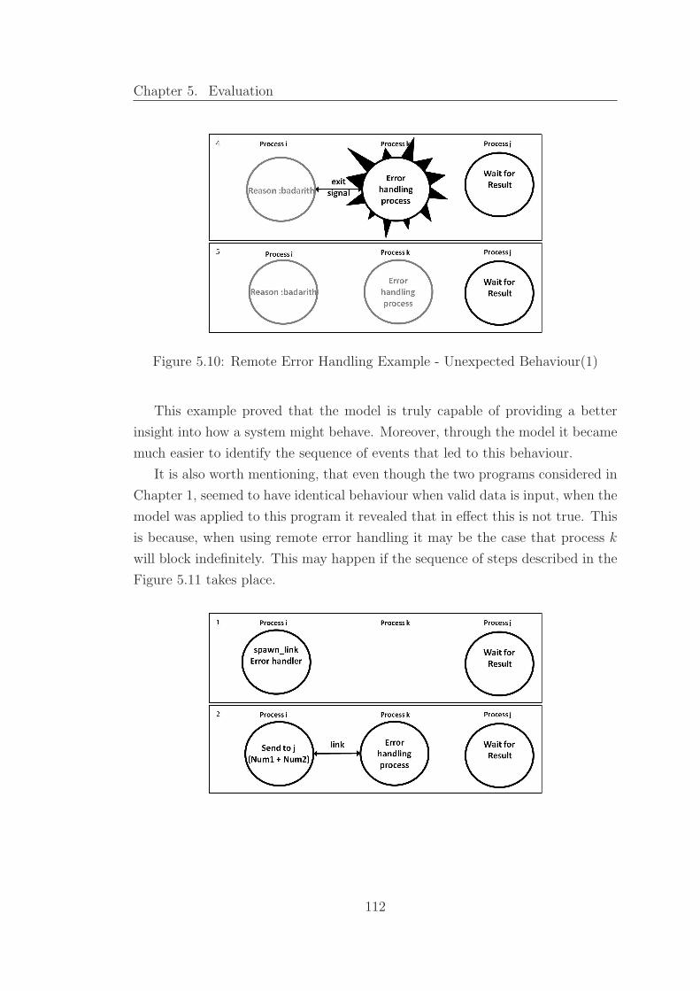
Chapter 5. Evaluation
Figure 5.10: Remote Error Handling Example - Unexpected Behaviour(1)
This example proved that the model is truly capable of providing a better
insight into how a system might behave. Moreover, through the model it became
much easier to identify the sequence of events that led to this behaviour.
It is also worth mentioning, that even though the two programs considered in
Chapter 1, seemed to have identical behaviour when valid data is input, when the
model was applied to this program it revealed that in effect this is not true. This
is because, when using remote error handling it may be the case that process k
will block indefinitely. This may happen if the sequence of steps described in the
Figure 5.11 takes place.
112

Chapter 5. Evaluation
Figure 5.11: Remote Error Handling Example - Unexpected Behaviour(2)
In the above diagram, process i terminates before process k has set its pro-
cess flag(4). Since the reason is set to normal, the received signal is ignored(5).
After receiving the signal, process k will set its process flag to true(6). Given
the fact that both process i and process j have terminated, process k will then
remain blocked waiting for the message describing the way process i terminates.
Through this simple case study, it became evident that the defined model
is able to provide a better insight into Erlang’s both local and remote error
handling constructs. As a result, whereas before it was somewhat difficult to truly
reason about Erlang’s behaviour in the presence of errors through the model it
became much easier to understand such behaviour. Moreover, the step-by-step
description of how Erlang programs are evaluated greatly helped to reveal the
cause of unexpected behaviour.
113

Chapter 5. Evaluation
5.4 Evaluation Results
This last section, outlines some facts that were observed during the evaluation
stage of this project. Primarily, it first gives a summary describing the results
that were obtained when measuring to what degree the model is faithful to actual
Erlang. Subsequently, the main limitations of the work done in this project are
discussed.
5.4.1 Accomplishments
In this section a table is presented summarizing all the different aspects of the
model that have been analysed in this chapter. Primarily it shows, if the model
is sound and/or complete with respect to the behaviour of actual Erlang. The
term soundness refers to the fact that the model can never describe a behaviour
which may never occur in reality. Completeness refers to the fact that the model
is able to represent all the possible ways actual Erlang may behave when using
that particular mechanism.
Erlang mechanismModel
Sound Complete
Local Error Handling - try-catch X X
Error Propagation - linking X X
Error Propagation - monitoring X
Explicit Error Signals X X
Order of Signal Evaluation X
Table 5.4: Soundness & Completeness of Model
Here, it is important to note that since in this project the evaluation approach
was not a formal one, the X symbol does not necessary imply that a particular
mechanism is 100% guaranteed to be sound or complete. However, the several
examples which were considered during the evaluation stage gave us a good indi-
cation if the behaviour of a specific Erlang mechanism as described by the model
is sound and/or complete.
This table shows that the defined model was found to be able to describe
soundly the behaviour of all the Erlang mechanisms that were considered. This
114

Chapter 5. Evaluation
is because when carrying out the evaluation it was never the case that the model
described a behaviour which can never occur in actual Erlang.
With respect to the model’s completeness, in some cases the model fell short to
describe all the possible ways an Erlang system may behave. For instance, when
using monitors, the model was not able to completely describe the behaviour of
actual Erlang when one particular process created multiple monitors of another
process. The model was also found not to be complete when it came to describing
the ordering in which sent signals are evaluated. This is because, whereas the
model assumes that all signals are evaluated in the same order in which they
are sent, in reality Erlang may sometimes evaluate the sent signals in a different
order.
However, even though the model is not complete through the evaluation stage
it became evident that by using the model we are now able to get a better
insight into how Erlang’s error handling mechanisms behave. In this chapter,
this fact became even more clear through the several number of test cases which
were carried out. In all these test cases the model was able to give a precise
description of how particular constructs behave.
Through the model it also became possible to get a good indication if two
systems are expected to behave in a similar way or not. For instance, in the
last case study, the model was able to show that although the program which
adopted remote error handling seemed to have an identical behaviour to the one
using local error handling, in truth the two programs may behave in a different
way.
5.4.2 Limitations
Even though, in most cases the defined semantics and designed evaluator are able
to faithfully mirror the behaviour of actual Erlang through the evaluation stage
it became apparent that they still suffer from some limitations.
5.4.2.1 A Single-node Semantics
One main limitation of the defined semantics is that they are only able of de-
scribing all possible behaviors of single-node systems. If these semantics were to
be used to describe the behaviour of distributed Erlang systems, the rules may
not be able to describe completely the different ways in which the system might
115

Chapter 5. Evaluation
behave. This is because, as claimed by [3], when dealing with distributed Erlang
systems, signal delivery is not immediate. In contrast, the defined semantics as-
sumes that all signals are received instantaneously. In order to better understand,
the implications of this latter fact let’s consider the following case:
Figure 5.12: Error signals - Distributed Systems
In the above system Process A, first sends an explicit exit signal to process C.
Subsequently, an error signal is sent to process B. Once process B receives the
exit signal it will terminate and an exit signal is sent to process C.
According to the defined semantics, process C will always terminate with
reason ‘first’ and process B will always terminate with reason ‘second’. This
is because in the defined semantics all exit signals are received and evaluated
immediately. However, in actual Erlang if all three processes were to be found
on different nodes, the exit signal delivery is not guaranteed to be instantaneous.
Therefore, even though process A will send the exit signal ‘first’ to process C
prior to sending an exit signal ‘second’ to process B, it is not guaranteed that
the ‘first’ signal arrives at C prior to the exit signal ‘second’. In actual fact, it
may very well be the case that process C terminates with reason ‘second’. This
kind of behaviour cannot be described through the presented semantics.
5.4.2.2 Simulation Time
Perhaps one of the main limitations of the designed evaluator is that in some
cases it may take a considerably long time to produce an output describing the
different ways the system may behave. The underlying cause lies in the fact
that the number of different interleavings that need to be checked will grow
exponentially to the size of the input system. As a result, the designed evaluator
116

Chapter 5. Evaluation
is only able to simulate the behaviour of small systems in a reasonable amount
of time.
5.5 Conclusion
This chapter evaluated the different aspects of this project. This was done by
considering a number of Erlang systems and comparing the behaviour of these
programs as described by the model against the way the same programs behaved
when run on the Erlang VM. This evalution strategy gave us a clear indication to
what extent the model is able to faithfully mirror the behaviour of actual Erlang.
Additionally, it also helped to expose the main benefits and limitations of the
defined model and evaluator.
117

6. Conclusion and Future Work
In this final chapter the benefits that have been achieved through this project will
be outlined. Subsequently, some improvements that could be done to the work
presented in this project are suggested.
6.1 Benefits Achieved
The following points outline the main results that were accomplished through the
defined semantic rules.
Offer a better insight - In the initial stage of this project it was not quite clear
how Erlang systems, especially those which made use of the remote error handling
constructs might behave. For instance, in Chapter 1, it was rather unclear why
the program which made use of the remote error handling constructs(Listing 1.2)
does not always behave in the same way as the one which uses local error han-
dling constructs(Listing 1.1). The model defined in this work has successfully
addressed these type of problems by providing precise and unambigious descrip-
tion of Erlang’s error handling constructs. As a result, as shown in the Evaluation
chapter, by applying the model on a particular Erlang systems it is now possible
to understand immediately why a system is behaving in a certain way.
Explain the cause of unexpected behaviour - The defined rules are capable
of providing a step-by-step description of how a system is evaluated possibly
revealing sequences of steps that may lead to unexpected outcomes. For instance,
with respect to the example described in Chapter 1, it is now clear why sometimes
the system which makes use of remote error handling constructs behaves in an
118

Chapter 6. Conclusion and Future Work
unexpected way and thus fails to handle any raised exceptions. This is because
through the defined model it is now possible to retrace the sequence of steps that
may cause the system to behave in an unexpected way.
Predict system’s behaviour - Prior to defining the model, the only way a
user could see how an Erlang system might behave was by executing it on the
Erlang VM. In fact, in the initial stage of this project, the difference in behaviour
between Listing 1.1 and Listing 1.2 could only be noted after the two systems
were run on the Erlang VM. Conversely, through the defined rules it has became
possible to see that the two systems might behave in different ways, without the
need of actually running the systems on the Erlang VM.
Lay the foundations of a semantic theory - This model is able to give a
good indication of whether or not a pair of systems are expected to have identical
behaviour. For instance, even though the pair of systems described in Chapter
1 seemed to have identical behaviour, the model was able to show that in actual
fact this was not the case. In fact, when the model was applied to the pair of
programs, it was able to bring to light the subtle difference that existed between
them. This fact indicates that the defined rules can act as a basis for defin-
ing notions of equivalence such as testing equivalence[26] and reduction barbed
congruence, which can later be justified through labelled transition systems and
bisimulations[24, 25].
6.2 Suggestions for Future Work
Even though the main objectives of this project have been met, there is still room
for improvement. In this section a number of suggestions that may be considered
for future work are presented.
6.2.1 Distributed-node Semantics
Following up this work, it would be interesting to study the behaviour of Erlang’s
error handling mechanisms when used in distributed systems. The rules defined
in this project are only able to accurately describe the behaviour of single-node
systems. Therefore, when considering the fact that in these days more emphasis is
being put on building distributed systems it would be quite beneficial to extend
119

Chapter 6. Conclusion and Future Work
the semantic rules defined here so as to be able to cater also for distributed
systems.
6.2.2 Extend chosen Erlang Subset
Another improvement that could be done to the semantics, is to modify Erlang’s
chosen subset so as to accept all constructs found in Core Erlang[2]. As claimed in
[3], Core Erlang represents a complete core fragment of Erlang. Therefore, if the
semantics is modified to operate on Core Erlang, it would be a great step towards
defining a complete semantics for Erlang. In addition, since there already exists a
compiler(HiPE compiler) which can automatically translate Erlang programs in
terms of Core Erlang, it will become possible to modify the designed evaluator to
accept ordinary Erlang programs instead of programs consisting only of constructs
found in the chosen subset. This is because the HiPE compiler could then be
used to translate the input fed to the evaluator in terms of Core Erlang prior to
simulating Erlang’s behaviour according to the defined semantics.
6.2.3 Improve Evaluator’s Efficiency
One major downside of the designed evaluator is that it may be rather slow when
simulating the behaviour of input systems. Even though some techniques have
already been adopted in order to improve its efficiency, it would be ideal to further
explore other modifications that could be made to make it more efficient. Perhaps,
one possible improvement would be that given the fact that the simulation of
different traces is independent of each other, they could easily be carried out in
parallel.
6.2.4 A semantic theory based around notions of equiva-
lence
The model defined in this work only provides the basis of a semantic theory.
Therefore, it would be interesting to extend this work so that given any two
Erlang systems it would be able to show if they are truly semantically equivalent
or not.
120

Chapter 6. Conclusion and Future Work
6.3 Conclusion
This project gave a closer insight into Erlang’s error handling mechanisms. A
formal semantic definition for these mechanisms was presented providing an ac-
curate and unambigious description of Erlang’s behaviour when dealing with
errors. These definitions have been animated through an evaluator which returns
a detailed description of all the possible different ways a particular Erlang system
may behave.
In order to better appreciate the usefulness of these formal definitions, the
behaviour of a number of different Erlang systems was described according to
the defined semantics. These descriptions were found to be really helpful in un-
derstanding why sometimes certain systems behaved in an unexpected way. In
addition, these descriptions were also able to approximate whether two syntacti-
cally different systems were truly semantically equivalent or not.
121

A.
Here are some steps that need to be followed in order to use the designed evalu-ator.
A.1 Prerequisites
• pdf reader eg. Acrobat Reader
• implementation of LaTeX eg. MiKTeX (listings package needed)
A.2 Using the Evaluator
In order to use the evaluator
1. Copy Evaluator Folder onto your computer.
2. Run the Evaluator.bat file.
3. In the command prompt enter the path where the “functions” file is found.This file should contain the necessary function definitions that are neededwhen running the Erlang system. The syntax of the input file should bequite similar to the one used when writing an Erlang module. In factthe only differences between an ordinary Erlang module file and the inputaccepted by the evaluator are that in the input file:
• the module and export constructs need not be included
• definitions of functions which share the same function name are notdelimeted by a ; but by a .
• the spawn link, spawn monitor and spawn functions do not expect themodule name parameter
• only the subset of Erlang as defined in Table 3.2 can be successfullyparsed
122

Appendix A.
Following there is a simple Erlang module and how it can be expressed
in terms of the evaluator’s input. The code in green, highlights the parts
which need to be removed or modified before an Erlang module is fed to
the evaluator.
Erlang Module:
-module(example1).
-export([init/1,sum/1,getSum/2]).
sum([]) -> 0;
sum([H|T]) -> H + sum(T).
getSum(Pid,List) -> Pid ! sum(List).
init(List) ->
spawn_link(?MODULE,getSum,[self(),List]),
receive
Sum -> Sum
end.
Evaluator’s input:
sum([]) -> 0.
sum([H|T]) -> H + sum(T).
getSum(Pid,List) -> Pid ! sum(List).
init(List) ->
spawn_link(getSum,[self(),List]),
receive
Sum -> Sum
end.
4. After entering the functions file path, enter the path of the file containing
the expression that in actual Erlang is input into Erlang’s shell.
5. In the command prompt then enter the name of the output file.
6. The system will then automatically create and open a pdf file containing a
detailed description of the different ways the system may behave.
123

Bibliography
[1] J. Magee & J. Kramer Concurrency : state models and Java programsWiley, 2006
[2] R. Carlsson, B. Gustavsson, E. Johansson, T. Lindgren, S. Nystrom,M.Pettersson, R. Virding Core Erlang 1.0.3 language specification, 2004
[3] K. Claessen, & H. Svensson A Semantics for Distributed Erlang ACM, 2005
[4] Nuseibeh, B.; , ”Ariane 5: Who Dunnit?,” Software, IEEE , vol.14, no.3,pp.15-16, May/Jun 1997
[5] W. N. Toy. Fault-tolerant design of local ess processors. In Proceedings ofIEEE, pages 11261145. IEEE Computer Society, 1982
[6] G. E. Moore Cramming more components onto integrated circuitsApril, 1965 URL ftp://download.intel.com/museum/Moores_Law/
Articles-Press_Releases/Gordon_Moore_1965_Article.pdf Date LastAccessed: 20th May 2011
[7] A. Silberschatz, P.B. Galvin, & G. Gagne Operating System Concepts JohnWiley & Sons, Inc, 2005
[8] J. Armstrong Making Reliable Distributed Systems in the Presencs of Soft-ware Errors Royal Institute of Technology, Stockholm, Sweden, 2003
[9] S. Nystrom Concurrency in Java and in Erlang Department of InformationTechnology, Uppsala University, Sweden, 2004
[10] S. Agarwal & P. Lakhina Erlang - Programming the Parallel WorldURL http://www.cs.ucsb.edu/ puneet/reports/erlang.pdf Date last ac-cessed: 20th May 2011
[11] J. A. Board Transputer research and applications, 2:NATUG-2 IOS PRESS,1990
[12] F. Cesarini & S. Thompson Erlang programming O’Reilly Media 2009
124

Bibliography
[13] H. Svensson & L.A. Fredlund A more accurate semantics for distributederlang. In Proceedings of the 2007 SIGPLAN workshop on ERLANG Work-shop (ERLANG ’07). ACM, 2007
[14] L.Fredlund Towards a semantics for Erlang Workshop on Foundations ofMobile Computation, Chennai, India, 1999
[15] H. Svensson, L.A. Fredlund & C.B. Earle A unified semantics for futureErlang . In Proceedings of the 9th ACM SIGPLAN workshop on Erlang(Erlang ’10). ACM, 2010
[16] L. A. Fredlund & H. Svensson McErlang: a model checker for a distributedfunctional programming language. SIGPLAN Not. 42, 9 (October 2007),125-136. ACM, 2007
[17] H. Svensson and L.A. Fredlund. Programming distributed erlang applica-tions: pitfalls and recipes. In Proceedings of the 2007 SIGPLAN workshopon ERLANGWorkshop (ERLANG ’07). ACM, New York, NY, USA, 37-42.2007.
[18] J. Barklund and R. Virding. Erlang 4.7.3 reference manual Draft (0.7),Ericsson Computer Science Laboratory, 1999.
[19] Aho, A.V., Sethi, R., & Ullman, J.D. (2003). Compilers principles, tech-niques, and tools. United States: Bell Telephone Laboratories.
[20] Scanner.hs Retrieved from http://www.cs.bris.ac.uk/Teaching/
Resources/COMS30122/haskell/Scan.hs Data last accessed: 30th April2011
[21] C.B. Earle, L.A. Fredlund, & J. Derrick. Verifying fault-tolerant Erlangprograms. In Proceedings of the 2005 ACM SIGPLAN workshop on Erlang(ERLANG ’05). 2005
[22] Q. H. DO & T.D. Ajakaiye Fault Injection Technique for Evaluating ErlangTest Suites 2009
[23] Erlang Reference Manual. Accessed from http://www.erlang.org/doc/
man/erlang.html Date last accessed: 20th May 2011
[24] D. Sangiorgi & D. Walker The π-calculus: A Theory of Mobile Processes.Cambridge, UK: Cambridge University Press, 2001
[25] R. Milner Communicating and Mobile Systems: The π-calculus. Cambridge,UK: Cambridge University Press,1999
[26] M. Hennessy Algebraic Theory of Processes The MIT Press, Boston 1988
125