
TOPOLOGICAL RECURSION FOR THE CONIFOLD …TOPOLOGICAL RECURSION FOR THE CONIFOLD TRANSITION OF A...
32
TOPOLOGICAL RECURSION FOR THE CONIFOLD TRANSITION OF A TORUS KNOT BOHAN FANG AND ZHENGYU ZONG Abstract. In this paper we prove a mirror symmetry conjecture based on the work of Brini-Eynard-Mari˜ no [4] and Diaconescu-Shende-Vafa [6]. This conjecture relates open Gromov-Witten invariants of the conifold transition of a torus knot to the topological recursion on the B-model spectral curve. Contents 1. Introduction 2 Outline 3 Acknowledgement 4 2. Torus knots and the resolved conifold 4 2.1. The conifold transition 4 2.2. Torus knots and Lagrangians in the deformed conifold 4 2.3. Lagrangians in the resolved conifold 6 3. Topological A-strings in the resolved conifold: Gromov-Witten theory 7 3.1. Equivariant cohomology of the resolved conifold 7 3.2. Equivariant Gromov-Witten invariants and their generating functions 8 3.3. The equivariant quantum cohomology of X 9 3.4. The A-model canonical coordinates and the Ψ-matrix 10 3.5. The equivariant quantum differential equation 11 3.6. The S -operator 11 3.7. The A-model R-matrix 13 3.8. The A-model graph sum 13 3.9. Open-closed Gromov-Witten invariants 15 3.10. Open-closed Gromov-Witten invariants as relative Gromov-Witten invariants I: the degree zero case 17 3.11. Open-closed Gromov-Witten invariants as relative Gromov-Witten invariants II: the general case 20 4. The spectral curve of a torus knot 23 4.1. Mirror curve and the disk invariants 23 4.2. Differential forms on a spectral curve 24 4.3. Higher genus invariants from Eynard-Orantin’s topological recursion 25 5. Mirror symmetry for open invariants with respect to L P,Q 27 5.1. Mirror theorem for genus 0 descendants 27 5.2. Mirror symmetry for disk invariants 28 5.3. Matching the graphs sums 29 5.4. Matching open leaves 29 References 31 1 arXiv:1607.01208v2 [math.AG] 6 Jan 2017
Transcript of TOPOLOGICAL RECURSION FOR THE CONIFOLD …TOPOLOGICAL RECURSION FOR THE CONIFOLD TRANSITION OF A...

TOPOLOGICAL RECURSION FOR THE CONIFOLD
TRANSITION OF A TORUS KNOT
BOHAN FANG AND ZHENGYU ZONG
Abstract. In this paper we prove a mirror symmetry conjecture based on
the work of Brini-Eynard-Marino [4] and Diaconescu-Shende-Vafa [6]. Thisconjecture relates open Gromov-Witten invariants of the conifold transition of
a torus knot to the topological recursion on the B-model spectral curve.
Contents
1. Introduction 2Outline 3Acknowledgement 42. Torus knots and the resolved conifold 42.1. The conifold transition 42.2. Torus knots and Lagrangians in the deformed conifold 42.3. Lagrangians in the resolved conifold 63. Topological A-strings in the resolved conifold: Gromov-Witten theory 73.1. Equivariant cohomology of the resolved conifold 73.2. Equivariant Gromov-Witten invariants and their generating functions 83.3. The equivariant quantum cohomology of X 93.4. The A-model canonical coordinates and the Ψ-matrix 103.5. The equivariant quantum differential equation 113.6. The S-operator 113.7. The A-model R-matrix 133.8. The A-model graph sum 133.9. Open-closed Gromov-Witten invariants 153.10. Open-closed Gromov-Witten invariants as relative Gromov-Witten
invariants I: the degree zero case 173.11. Open-closed Gromov-Witten invariants as relative Gromov-Witten
invariants II: the general case 204. The spectral curve of a torus knot 234.1. Mirror curve and the disk invariants 234.2. Differential forms on a spectral curve 244.3. Higher genus invariants from Eynard-Orantin’s topological recursion 255. Mirror symmetry for open invariants with respect to LP,Q 275.1. Mirror theorem for genus 0 descendants 275.2. Mirror symmetry for disk invariants 285.3. Matching the graphs sums 295.4. Matching open leaves 29References 31
1
arX
iv:1
607.
0120
8v2
[m
ath.
AG
] 6
Jan
201
7

2 BOHAN FANG AND ZHENGYU ZONG
1. Introduction
The Chern-Simons theory of a knot in S3 [36] is related to topological stringsin T ∗S3 and, through a conifold transition, to topological strings in the resolvedconifold X = OP1(−1)⊕OP1(−1) [7,34,37]. We briefly review the related backgroundand state our result in this section.1
Let A be a connection on S3 for the gauge group G = U(N) and R be a rep-resentation of G. The Chern-Simons action functional is the following (where k isthe coupling constant)
S =k
4π∫S3
TrR (A ∧ dA +2
3A ∧A ∧A) .
The partition function of this theory is defined by path-integrals in physics
Z(S3) = ∫ DAe
√−1S(A).
Let K ≅ S1 S3 be a framed, oriented knot2. In physics, the normalized vacuumexpectation value (vev) is
WR(K) =1
Z(S3)∫ DAe
√−1S(A)TrRUK ,
where UK is the holonomy around K. This definition also relies on path-integral. Inmathematics, for example, when R is the fundamental representation of G = U(N),WR(K) is related to the HOMFLY polynomial PK(q, λ) of K as below
WR(K) = λλ
12 − λ−
12
q12 − q−
12
PK(q, λ),
where
q = e2π√
−1k+N , λ = qN .
Under the large-N duality and the conifold transition, the gauge theory in-variant WR(K) is conjecturally related to the open Gromov-Witten theory ofX = OP1(−1) ⊕ OP1(−1) [7, 34] with Lagrangian boundary condition LK . WhenK is an unknot, the conjecture can be precisely formulated as the famous Marino-Vafa formula concerning Hodge integrals and is later proved [27,31,33].
Although the general construction of LK out of K other than unknots was notvery clear in the beginning, later the construction [20, 21, 35] provided recipes forLK . In this paper, we follow Diaconescu-Shende-Vafa’s construction [6] for analgebraic knot K, which produces a Maslov index 0 non-compact Lagrangian LK ≅
S1 ×R2 in X .Open Gromov-Witten theory is usually difficult to define for (X , LK). When K
is an unknot, LK belongs to a class of Lagrangians called Aganagic-Vafa branes[1, 2] (Harvey-Lawson type Lagrangian). The open Gromov-Witten invariants for(X , LK) in this situation are defined in [19,26]. When K is a torus knot, i.e. a knotthat can be realized on a real torus in S3, one can still use the localization techniqueto define such open Gromov-Witten invariants [6]. In [6], Diaconescu-Shende-Vafaalso prove the conjecture on the correspondence between HOMFLY polynomialsand open Gromov-Witten invariants.
1For a comprehensive review, see e.g. [29,30].2The construction also works for links – we restrict ourselves to knots in this paper.

TOPOLOGICAL RECURSION FOR TORUS KNOTS 3
The topological A-type string theory on X has mirror symmetry. The B-model isa spectral curve. When the Lagrangian LK in X is an Aganagic-Vafa brane, i.e. theconifold transition of an unknot, all genus Gromov-Witten open-closed invariantsare obtained from Eynard-Orantin’s topological recursion of a particular spectralcurve [3,10–12]. In [4], Brini-Eynard-Marino propose a modified spectral curve fora torus knot KP,Q with coprime (P,Q). They conjecture that this curve should bethe correct B-model topological strings large-N dual to the knot K. Combined withthe construction of A-model open Gromov-Witten invariants in [6], one naturallyexpects the Eynard-Orantin recursion should predict these open GW invariants for(X , LK).
More precisely, we can collect genus g, n boundary components open Gromov-Witten invariants and compose them into a generating function Fg,n(X1, . . . ,Xn, τ1)(see Section 3.9). On the other hand, the spectral curve Cq, roughly speaking, isthe following curve
Cq = 1 +U + V + qUV = 0,
with a holomorphic function X = UQV P on Cq.Eynard-Orantin’s recursion is a recursive algorithm that produces all genus open
invariants of this spectral curve (see Section 4.3). From the recursion, we get a
symmetric meromophic n-form ωg,n on (Cq)n. The variable η = X
1Q is a local
coordinate around (U,V ) = (0,−1). One can integrate the expansion of ωg,n inη1, . . . , ηn around this point and define
Wg,n(η1, . . . , ηn, q) = ∫η1
0. . .∫
ηn
0ωg,n.
The mirror symmetry for (X , LK) says the following
Theorem (Conjecture from Brini-Eynard-Marino, Diaconescu-Shende-Vafa [4,6]).
Under τ1 = log q and Xk = ηQk , the power series expansion of the open Gromov-Witten amplitude Fg,n(τ1;X1, . . . ,Xn) in X1, . . . ,Xn is the part in the power seriesexpansion of (−1)g−1+nQnWg,n(q, η1, . . . , ηn) whose degrees of each ηk are divisibleby Q.
Remark 1.1. In [18], Gu-Jockers-Klemm-Soroush argue that the B-model spectralcurve of a knot is defined by the augmentation polynomial. If we choose suchaugmentation polynomial, although more complicated than the spectral curve Cqhere, we do not need to discard terms with degrees divisible by Q. The authors hopethe Main Theorem here will lead to the prediction by the augmentation variety. Anexperimental computation of augmentation polynomial by localization of open GWinvariants is in [28].
Outline. In Section 2 we recall the construction in [6]. Starting from an algebraicknot K in S3 we will construct a Lagrangian LK in X . In Section 3 we define openGromov-Witten invariants with respect to (X , LK) for a torus knot K in two ways:by localization in the moludi space of maps from bordered Riemann surfaces, andby relative Gromov-Witten invariants. We also express the generating functionsfor these invariants in graph sums. In Section 4 we discuss the B-model mirrorto (X , LK) as a spectral curve Cq, and express the Eynard-Orantin invariants interms of graph sums. Finally, in Section 5 we prove the all genus mirror symmetrybetween (X , LK) and Cq, based on the localization computation on disk invariants,genus 0 mirror theorem and graph sum formulae.

4 BOHAN FANG AND ZHENGYU ZONG
Acknowledgement. We would like to thank Chiu-Chu Melissa Liu for very help-ful discussion and the wonderful collaboration in many related projects – thoseprojects are indispensable to this one. We also thank her for the constructionof disk invariants using relative Gromov-Witten invariants in our case. The firstauthor would like to thank Sergei Gukov for the discussion on the localization com-putation for torus knots. The work of BF is partially supported by the RecruitmentProgram of Global Experts in China and a start-up grant at Peking University. Thework of ZZ is partially supported by the start-up grant at Tsinghua University.
2. Torus knots and the resolved conifold
In this paper, we consider the conifold Y0 which is a hypersurface in C4 definedby the following equation:
2.1. The conifold transition.
xz − yw = 0.
Here x, y, z,w are standard coordinates in C4. The conifold Y0 has a singularityat the origin x = y = z = w = 0. The deformed conifold Yδ defined by the followingequation:
xz − yw = δ,
where δ ∈ C∖ 0. Then Yδ is a smooth hypersurface in C4. Consider the standardsymplectic form on C4:
ωC4 =
√−1
2(dx ∧ dx + dy ∧ dy + dz ∧ dz + dw ∧ dw).
The symplectic form on Yδ is ωYδ = ωC4 ∣Yδ . Then Yδ becomes a symplectic manifoldand there exists a symplectomorphism φδ ∶ Yδ → T ∗S3, where T ∗S3 is the cotangentbundle of the 3-sphere. Consider the anti-holomorphic involution for δ ≥ 0.
I ∶ C4→ C4(1)
(x, y, z,w) ↦ (z,−w, x,−y).
Then Yδ is preserved by I. When δ > 0, the fixed locus Sδ of the induced anti-holomorphic involution Iδ on Yδ is isomorphic to a 3-sphere of radius
√δ and φδ(Sδ)
is the zero section of T ∗S3. When δ = 0, S0 is the singular point of Y0. But westill have a symplectomorphism φ0 ∶ Y0 ∖0→ T ∗S3 ∖S3, where we view S3 as thezero section of T ∗S3.
The second way to smooth the singularity of Y0 is to consider the resolved conifoldX . We consider the blow-up of C4 along the subspace (x, y, z,w)∣y = z = 0. LetX be the resolution of Y0 under the blow-up. Then X is isomorphic to the localP1:
X ≅ [OP1(−1)⊕OP1(−1)→ P1].
If we view X as a subspace of C4×P1, then X is defined by the following equations:
(2) xs = wt, ys = zt,
where [s ∶ t] is the homogeneous coordinate on P1. The resolution p ∶ X → Y0 isgiven by contracting the base P1 in X . We say that X and Yδ are related by theconifold transition.
2.2. Torus knots and Lagrangians in the deformed conifold.

TOPOLOGICAL RECURSION FOR TORUS KNOTS 5
2.2.1. Conormal bundle of a knot in S3. Consider a knot K ⊂ S3. Let M be thetotal space of the conormal bundle N∗
K of K in S3. Then M can be embedded intoT ∗S3 as a Lagrangian submanifold and the intersection of M with the zero sectionof T ∗S3 is the knot K. Recall that we have a symplectomorphism for δ > 0
φδ ∶ Yδ → T ∗S3
and φδ(Sδ) is the zero section of T ∗S3. So φ−1δ (M) is a Lagrangian submanifold of
Yδ and the intersection φ−1δ (M)∩Sδ is a knot in Sδ which is isomorphic to K ⊂ S3.
Our goal is to construct a Lagrangian LK in the resolved conifold X , which insome sense corresponds to the knot K under the conifold transition. The difficultyhere is that when δ → 0, the subset Sδ ⊂ Yδ shrinks to a point which is the singularpoint of the conifold Y0. Since the intersection φ−1
δ (M) ∩ Sδ is nonempty, theLagrangian φ−1
δ (M) becomes singular in the limit δ → 0. So it is not easy toconstruct a Lagrangian LK in the resolved conifold X which is the “transition” ofφ−1δ (M).
We follow the solution to the above problem for algebraic knots in [6] (see also[20] for a more general construction), where the knot K is “lifted”to a path γ inT ∗S3 which does not intersect with the zero section. The Lagrangian M is alsolifted to a new Lagrangian containing γ and it does not intersect with the zerosection either. Then the “transition” LK of φ−1
δ (M) can be naturally constructed.For completeness, we review this process in Section 2.2.2 and Section 2.3.
2.2.2. Lifting of the torus knots. We restrict ourselves to torus knots. Let P,Q betwo fixed coprime positive integers. Let f(x, y) = xP −yQ and consider the algebraiccurve
f(x, y) = 0
in C2. For small r, the intersection of the curve f(x, y) = 0 with the 3-sphere∣x∣2 + ∣y∣2 = r represents a knot in S3 which is called the (P,Q)-torus knot. Wedenote this knot by K.
We want to consider the 1-dimensional subvariety Zδ ⊂ Yδ defined by the com-plete intersection of Yδ with
(3) f(x, y) = 0, f(z,−w) = 0.
The subvariety Zδ is disconnected in general and its connected components can bedescribed as follows. The Equations (3) together with the defining equation of Yδimplies
(xz)P − (δ − xz)Q = 0.
Let xz = ξ and then ξ is a solution to the equation uP − (δ − u)Q = 0 for u. Eachsolution ξ of this equation determines a connected component of Zδ of the form
(x, y, z,w) = (tQ, tP , ξt−Q, (δ − ξ)t−P )
for t ∈ C∗.Since the coefficients of f are real, Zδ is preserved under the anti-holomorphic
involution I. Each connected component of the intersection Zδ ∩ Sδ is isomorphicto the knot K in Sδ ≅ S
3. Let
Pa = (u, v) ∈ T ∗S3∣ ∣v∣ = a
be the sphere bundle of radius a in T ∗S3 under standard metric of the unit sphereS3. Suppose there exits an irreducible component Cδ of Zδ such that the inter-section Cδ ∩ Sδ is isomorphic to the knot K in Sδ. Then for small a > 0, the

6 BOHAN FANG AND ZHENGYU ZONG
intersection φδ(Cδ) ∩ Pa is nontrivial and the projection π(φδ(Cδ) ∩ Pa) is equalto φδ(Cδ ∩ Sδ) ⊂ S3 which is the torus knot K. Here π ∶ T ∗S3 → S3 is the pro-jection map. Let γa ∶ S1 → T ∗S3 be the path φδ(Cδ) ∩ Pa and for t ∈ S1 letγa(t) = (g(t), h(t)) ∈ T ∗S3. Then the path (g(t),0) ∈ S3 is the knot K. Theconormal bundle N∗
K is defined as
(u, v) ∈ T ∗S3∶ u = g(t), ⟨v, g′(t)⟩ = 0,
where g′(t) is the derivative of g and ⟨, ⟩ is the natural pairing between tangentand cotangent vectors. As we discussed in Section 2.2.1, the conormal bundle N∗
K
is not what we want. Instead, we consider the Lagrangian Mγa ⊂ T∗S3 defined as
(4) (u, v) ∈ T ∗S3∶ u = g(t), ⟨v − h(t), g′(t)⟩ = 0.
The Lagrangian Mγa is obtained from N∗K by fiberwisely translating N∗
K by thecotangent vector h(t). We denote φ−1
δ (Mγa) by Mδ.When δ = 0, Z0 has two special irreducible components C± defined by
f(x, y) = 0, z = w = 0
andf(z,−w) = 0, x = y = 0
respectively. Both of C± meet the singular point of Y0 and the anti-holomorphicinvolution I0 exchanges C±. Consider the path γ+ defined by intersection φ0(C
+ ∖
0) ∩ Pa. Then by the construction in Equation (4), we obtain the correspond-ing Lagrangian Mγ+ in T ∗S3 and we denote φ−1
0 (Mγ+) by M0. For small δ > 0,there exists an irreducible component Cδ of Zδ such that there exists a connectedcomponent γδ of the intersection φδ(Cδ) ∩ Pa which specializes to γ+ when δ → 0.Therefore we obtain a family of Lagrangians Mδ which specializes to M0 whenδ → 0.
2.3. Lagrangians in the resolved conifold. For ε ≥ 0, we consider the symplec-tic form (ωC4+ε2ωP1) on C4×P1. By equation (2), we can view the resolved conifoldX as a subvariety in C4×P1. We define the symplectic form ωX ,ε (degenerate whenε = 0) on X by
ωX ,ε ∶= (ωC4 + ε2ωP1) ∣X .
Let B(ε) = (y, z) ∈ C2 ∣ ∣y∣2 + ∣z∣2 ≤ ε2 ⊂ C2 be the ball of radius ε. Consider theradial map ρε ∶ C2 ∖ 0→ C2 ∖B(ε),
ρε(y, z) =
√∣y∣2 + ∣z∣2 + ε2√
∣y∣2 + ∣z∣2(y, z).
Let %ε = idC2 ×ρε ∶ C2×(C2∖0)→ C2×(C2∖B(ε)). Then %ε preserves the conifoldY0 and it maps Y0 ∖ 0 to Y0(ε) ∶= Y0 ∖ (Y0 ∩ (C2 ×B(ε))). By the results in [32]and [6], the map
ψε ∶= %ε ∣Y0∖0 p ∣X∖P1 ∶ X ∖ P1→ Y0(ε)
is a symplectomorphism.Define the path γ+ε by
γ+ε ∶= φ0 %ε φ−10 γ+ ∶ S1
→ T ∗S3.
By applying the construction in (4) to the path γ+ε , we obtain a Lagrangian Mγ+ε
in T ∗S3. Then we define the Lagrangian Lε in the resolved conifold X to be
Lε ∶= ψ−1ε (φ−1
0 (Mγ+ε )).

TOPOLOGICAL RECURSION FOR TORUS KNOTS 7
The Lagrangian Lε will be used to define the open Gromov-Witten invariants inSection 3. Sometimes we omit the parameter ε and denote Lε by LK for the torusknot K, or simply by LP,Q. Let Xε be X equipped with the Kahler structure ωX ,εfor ε ≥ 0, which is degenerate when ε = 0. We summarize the construction as thefollowing diagram ([6, Equation 2.17]). Notice that the roles of X ,Y and L,Mare reversed from [6]. In the diagram, the wiggly arrow for Xε means changingthe Kahler structure ωX ,ε while keeping the underlying complex manifold X . Thewiggly arrow for Yδ means changing the deformation parameter δ, which causes Yδto collapse to Y0 when δ = 0. Here p∣L0 is a diffeomorphism between L0 and M0.
X0 Xε
Yδ Y0 L0 Lε
Mδ M0
p
p
3. Topological A-strings in the resolved conifold: Gromov-Wittentheory
3.1. Equivariant cohomology of the resolved conifold. Let X ≅ [OP1(−1) ⊕OP1(−1) → P1] be the resolved conifold given by the equation xs = wt, ys = ztwhere [s ∶ t] are the homogeneous coordinates on P1. Consider the 1-dimensionaltorus TP,Q ≅ C∗ which acts on X in the following way. Let torus TP,Q act on P1 by
t ⋅ [s ∶ t] = [t−P−Qs ∶ t].
Then there are two TP,Q−fixed points p0 = [0 ∶ 1],p1 = [1 ∶ 0]. Let ι0 ∶ p0 X andι1 ∶ p1 X be the inclusion maps of p0 and p1 respectively.
We lift this action to an TP,Q action on X by choosing the weights of the fibersof each O(−1) at p0,p1 to be P,−Q and Q,−P respectively. Let
(5) RTP,Q ∶=H∗TP,Q
(pt;C) = C[v]
be the TP,Q−equivariant cohomology of a point. Then the TP,Q−equivariant coho-mology ring H∗
TP,Q(X ;C) can be written as
(6) H∗TP,Q
(X ;C) = C[v,HTP,Q]/⟨HTP,Q(HTP,Q − (P +Q)v)⟩.
Here we have degHTP,Q = deg v = 2 and HTP,Q ∣p0= 0,HTP,Q ∣p1= (P +Q)v.On the other hand, we define
φ0 ∶ =[p0]
eTP,Q(Tp0X )=
(HTP,Q − (P +Q)v)(HTP,Q − P v)(HTP,Q −Qv)
−(P +Q)vP vQv=HTP,Q − (P +Q)v
−(P +Q)v
φ1 ∶ =[p1]
eTP,Q(Tp1X )=HTP,Q(HTP,Q − P v)(HTP,Q −Qv)
(P +Q)vP vQv=
HTP,Q
(P +Q)v,
where [pα] is the equivariant Poincare dual of pα. Then φ0, φ1 is a basis ofH∗TP,Q
(X ;C)⊗C[v] C(v). We have
(7) φα ∪ φβ = δαβφα.

8 BOHAN FANG AND ZHENGYU ZONG
Therefore φ0, φ1 is a canonical basis ofH∗TP,Q
(X ;C)⊗C[v]C(v). The TP,Q−equivariant
Poincare pairing is given by
(8) (φα, φβ)TP,Q =δαβ
∆α, α, β ∈ 0,1,
where ∆α = eTP,Q(TpαX ) = (−1)α+1(P +Q)PQv3, α = 0,1.The dual basis φα are φα = ∆αφα = [pα] under the TP,Q−equivariant
Poincare pairing. The normalized canonical basis φ0, φ1 is defined to be φα =√
∆αφα. Then we have
(9) (φα, φβ)TP,Q = δαβ , α, β ∈ 0,1.
Let STP,Q be a finite extension of the field C(v) by including√
∆α, α = 0,1. Then
φ0, φ1 is a basis of
(10) H∗TP,Q
(X ;C)⊗C[v] STP,Q .
3.2. Equivariant Gromov-Witten invariants and their generating func-tions. Let d ∈ H2(X ,Z) be an effective curve class. Let Mg,n(X , d) be the mod-uli space of genus g, n-pointed, degree d stable maps to X . Given γ1, . . . , γn ∈
H∗TP,Q
(X ,C) and a1, . . . , an ∈ Z≥0, we define genus g, degree d TP,Q-equivariant
descendant Gromov-Witten invariants of X :
⟨τa1(γ1) . . . τan(γn)⟩X ,TP,Qg,n,d ∶= ∫
[Mg,n(X ,d)TP,Q ]vir
∏nj=1 ψ
ajj ev∗j (γj) ∣
Mg,n(X ,d)TP,Q
eTP,Q(Nvir)
where evj ∶Mg,n(X,d)→ X is the evaluation at the j-th marked point, which is a
TP,Q-equivariant map, Mg,n(X , d)TP,Q is the TP,Q-fixed locus, and eTP,Q(N
vir) isthe TP,Q-equivariant Euler class of the virtual normal bundle. We also define genusg, degree d primary Gromov-Witten invariants:
⟨γ1, . . . , γn⟩X ,TP,Qg,n,d ∶= ⟨τ0(γ1)⋯τ0(γn)⟩
X ,TP,Qg,n,d .
Define the Novikov ring
Λnov ∶=C[E(X )] = ∑
d∈E(X)
cdQd∶ cd ∈ C,
where E(X ) is the set of effective curve classes which is identified with the set ofnonnegative integers in our case. We also define the following double correlatorwith primary insertions:
⟪γ1ψa1 ,⋯, γnψ
an⟫X ,TP,Qg,n ∶=
∞
∑m=0
∑d∈E(X)
Qd
m!⟨γ1ψ
a1 ,⋯, γnψan , tm⟩
X ,TP,Qg,n+m,d
where Qd ∈ C[E(X )] ⊂ Λnov is the Novikov variable corresponding to d ∈ E(X ), and
t ∈H∗TP,Q
(X ;C)⊗RTP,Q STP,Q . Let t = t01 + t1HTP,Q = t0φ0 + t1φ1. As a convention,
we use τ ∈H∗TP,Q
(X ;C) to denote a class in degree 2. Then τ = τ01+τ1HTP,Q where
τ1 ∈ C, and τ0 is degree 2 in H∗TP,Q
(pt).
For j = 1, . . . , n, introduce formal variables
uj = uj(z) = ∑a≥0
(uj)aza

TOPOLOGICAL RECURSION FOR TORUS KNOTS 9
where (uj)a ∈H∗TP,Q
(X ;C)⊗RTP,Q STP,Q . Define
⟪u1, . . . ,un⟫X ,TP,Qg,n = ⟪u1(ψ), . . . ,un(ψ)⟫
X ,TP,Qg,n
= ∑a1,...,an≥0
⟪(u1)a1ψa1 ,⋯, (un)anψ
an⟫X ,TP,Qg,n .
3.3. The equivariant quantum cohomology of X. In order to define the equi-variant quantum cohomology of X , we consider the three-point double correlator
⟪a, b, c⟫X ,TP,Q0,3 for a, b, c ∈ H∗
TP,Q(X ) ⊗RTP,Q STP,Q . Then by divisor equation, we
have
(11) ⟪a, b, c⟫X ,TP,Q0,3 ∈ STP,QJQK,
where Q =Qet1
. We define quantum product ⋆t by
(12) (a ⋆t b, c)X ,TP,Q ∶= ⟪a, b, c⟫X ,TP,Q0,3 .
Set
ΛTP,Qnov ∶= STP,Q ⊗C Λnov = STP,QJE(X )K.
Then H ∶=H∗TP,Q
(X ; ΛTP,Qnov ) is a free Λ
TP,Qnov -module of rank 2. Any point t ∈H can
be written as t = ∑1α=0 t
αφi . We have
H = Spec(ΛTP,Qnov [t0, t1]).
Let H be the formal completion of H along the origin:
H ∶= Spec(ΛTP,Qnov Jt0, t1K).
Let OH be the structure sheaf on H, and let TH be the tangent sheaf on H. Then
TH is a sheaf of free OH -modules of rank 2. Given an open set in H,
TH(U) ≅⊕α
OH(U)∂
∂tα.
The quantum product and the TP,Q-equivariant Poincare pairing defines the struc-
ture of a formal Frobenius manifold on H:
∂
∂tα⋆t
∂
∂tα′=∑
β
⟪φα, φα′ , φβ⟫X ,TP,Q0,3
∂
∂tβ∈ Γ(H,TH).
(∂
∂tα,∂
∂tα,)X ,TP,Q = δα,α′ .
The set of global sections Γ(H,T H) is a free OH(H)-module of rank 2:
Γ(H,T H) = ⊕α=0,1
OH(H)∂
∂tα.
Under the quantum product ⋆t, the triple (Γ(H,T H),⋆t, (, )X ,TP,Q) is a Frobenius
algebra over the ring OH(H) = ΛTP,Qnov Jt0, t1K. The triple (Γ(H,T H),⋆t, (, )X ,TP,Q)
is called the quantum cohomology of X and is denoted by QH∗TP,Q
(X ).
The semi-simplicity of the classical cohomologyH∗TP,Q
(X ;C)⊗RTP,Q STP,Q implies
the semi-simplicity of the quantum cohomology QH∗TP,Q
(X ). In fact, there exists
a canonical basis φ0(t), φ1(t) of QH∗TP,Q
(X ) characterized by the property that
(13) φα(t)→ φα, when t,Q→ 0, α = 0,1.

10 BOHAN FANG AND ZHENGYU ZONG
We denote φα(t) to be the dual basis to φα(t) with respect to the metric(, )X ,TP,Q . See [23] for more general discussions on the canonical basis.
3.4. The A-model canonical coordinates and the Ψ-matrix. The canonicalcoordinates uα = uα(t)∣α = 0,1 on the formal Frobenius manifold H are charac-terized by
(14)∂
∂uα= φα(t).
up to additive constants in ΛTP,Qnov . We choose canonical coordinates such that they
lie in STP,Q[t1]JQ, t0K and vanish when Q = 0, t0 = t1 = 0. Then uα −
√∆αtα ∈
STP,Q[t1]JQ, t0K and vanish when Q = 0, t0 = 0.
We define ∆α(t) ∈ STP,QJQ, t0K by the following equation:
(φα(t), φα′(t))X ,TP,Q =δα,α′
∆α(t).
Then ∆α(t) → ∆α in the large radius limit Q, t0 → 0. The normalized canonical
basis of (H,⋆t) is
φα(t) ∶=√
∆α(t)φα(t)∣α = 0,1.
They satisfy
φα(t) ⋆t φα′(t) = δα,α′√
∆α(t)φα(t), (φα(t), φα′(t))X ,TP,Q = δα,α′ .
(Note that√
∆α(t) =√
∆α⋅
√∆α(t)
∆α , where√
∆α ∈ STP,Q and√
∆α(t)∆α ∈ STP,QJQ, t0K,
so√
∆α(t) ∈ STP,QJQ, t0K.) We call φα(t)∣α = 0,1 the quantum normalized canon-
ical basis to distinguish it from the classical normalized canonical basis φα∣α =
0,1. The quantum canonical basis tends to the classical canonical basis in the
large radius limit: φα(t)→ φα as Q, t0 → 0.Let Ψ = (Ψ α
α′ ) be the transition matrix between the classical and quantumnormalized canonical bases:
(15) φα′ = ∑α=0,1
Ψ αα′ φα(t).
Then Ψ is an 2 × 2 matrix with entries in STP,QJQ, t0K, and Ψ → 1 (the iden-
tity matrix) in the large radius limit Q, t0 → 0. Both the classical and quantumnormalized canonical bases are orthonormal with respect to the TP,Q-equivariantPoincare pairing ( , )X ,TP,Q , so ΨTΨ = ΨΨT = 1, where ΨT is the transpose of Ψ,or equivalently
∑β=0,1
Ψ αβ Ψ α′
β = δα,α′
Equation (15) can be rewritten as
∂
∂tα′= ∑α=0,1
Ψ αα′
√∆α(t)
∂
∂uα
which is equivalent to
(16)duα
√∆α(t)
= ∑α′=0,1
dtα′
Ψ αα′ .

TOPOLOGICAL RECURSION FOR TORUS KNOTS 11
3.5. The equivariant quantum differential equation. We consider the Dubrovinconnection ∇z, which is a family of connections parametrized by z ∈ C ∪ ∞, on
the tangent bundle TH of the formal Frobenius manifold H:
∇zα =
∂
∂tα−
1
zφα⋆t
The commutativity (resp. associativity) of ∗t implies that ∇z is a torsion free (resp.flat) connection on TH for all z. The equation
(17) ∇zµ = 0
for a section µ ∈ Γ(H,TH) is called the TP,Q-equivariant quantum differential equa-tion (TP,Q-equivariant QDE). Let
Tf,z
H⊂ TH
be the subsheaf of flat sections with respect to the connection ∇z. For each z, T f,zH
is a sheaf of ΛTP,Qnov -modules of rank 2.
A section L ∈ End(TH) = Γ(H,T ∗H⊗ TH) defines a OH(H)-linear map
L ∶ Γ(H,TH) =⊕α
OH(H)∂
∂tα→ Γ(H,TH)
from the free OH(H)-module Γ(H,TH) to itself. Let L(z) ∈ End(TH) be a familyof endomorphisms of the tangent bundle TH parametrized by z. L(z) is called a
fundamental solution to the TP,Q-equivariant QDE if the OH(H)-linear map
L(z) ∶ Γ(H,TH)→ Γ(H,TH)
restricts to a ΛTP,Qnov -linear isomorphism
L(z) ∶ Γ(H,T f,∞H ) =⊕α
ΛTP,Qnov
∂
∂tα→ Γ(H,T f,zH ).
between rank 2 free ΛTP,Qnov -modules.
3.6. The S-operator. The S-operator is defined as follows. For any cohomologyclasses a, b ∈H∗
TP,Q(X ; STP,Q),
(a,S(b))X ,TP,Q = (a, b)X ,TP,Q + ⟪a,b
z − ψ⟫X ,TP,Q0,2
whereb
z − ψ=
∞
∑i=0
bψiz−i−1.
The S-operator can be viewed as an element in End(TH) and is a fundamentalsolution to the TP,Q-equivariant big QDE (17). The proof for S being a fundamentalsolution can be found in [5].
Remark 3.1. One may notice that since there is a formal variable z in the defini-tion of the TP,Q-equivariant big QDE (17), one can consider its solution space overdifferent rings. Here the operator S = 1 + S1/z + S2/z
2 + ⋯ is viewed as a formalpower series in 1/z with operator-valued coefficients.

12 BOHAN FANG AND ZHENGYU ZONG
Remark 3.2. By divisor equation and string equation, we have
(a, b)X ,TP,Q+⟪a,b
z − ψ⟫X ,TP,Q0,2 = (a, be(t
01+t1H)/z)X ,TP,Q+∑
d>0
Qdedt1
⟨a,be(t
01+t1H)/z
z − ψ⟩X ,TP,Q0,2,d .
In the above expression, if we fix the power of z−1, then only finitely many terms in
the expansion of e(t01+t1H)/z contribute. Therefore, the factor edt
1
can play the role
of Qd and hence the restriction ⟪a, bz−ψ
⟫X ,TP,Q0,2 ∣Q=1 is well-defined. So the operator
S ∣Q=1 is well-defined.
Definition 3.3 (TP,Q-equivariant J-function). The TP,Q-equivariant big J-functionJTP,Q(z) is characterized by
(JTP,Q(z), a)X ,TP,Q = (1,S(a))X ,TP,Q
for any a ∈H∗TP,Q
(X; STP,Q). Equivalently,
JTP,Q(z) = 1 +∑α
⟪1,φα
z − ψ⟫X ,TP,Q0,2 φα.
We consider several different (flat) basis for H∗TP,Q
(X ; STP,Q):
(1) The classical canonical basis φα∣α = 0,1.(2) The basis dual to the classical canonical basis with respect to the TP,Q-
equivariant Poincare pairing: φα = ∆αφα∣α = 0,1.
(3) The classical normalized canonical basis φα =√
∆αφα∣α = 0,1 which is
self-dual: φα = φα∣α = 0,1.
For α,α′ ∈ 0,1, define
Sα′
α(z) ∶= (φα,S(φα)).
Then (Sα′
α(z)) is the matrix of the S-operator with respect to the canonical basisφα∣α = 0,1:
(18) S(φα) = ∑α′=0,1
φα′Sα′
α(z).
For α,α′ ∈ 0,1, define
S αα′ (z) ∶= (φα′ ,S(φ
α)).
Then (S αα′ ) is the matrix of the S-operator with respect to the bases φα∣α = 0,1
and φα∣α = 0,1:
(19) S(φα) = ∑α′=0,1
φα′
S αα′ (z).
Introduce
Sz(a, b) = (a,S(b))X ,TP,Q ,
Vz1,z2(a, b) =(a, b)X ,TP,Qz1 + z2
+ ⟪a
z1 − ψ1,
b
z2 − ψ2⟫X ,TP,Q0,2 .
A well-known WDVV-like argument says
(20) Vz1,z2(a, b) =1
z1 + z2∑i
Sz1(Ti, a)Sz2(Ti, b),

TOPOLOGICAL RECURSION FOR TORUS KNOTS 13
where Ti is any basis of H∗TP,Q
(X ; STP,Q) and T i is its dual basis. In particular,
Vz1,z2(a, b) =1
z1 + z2∑α=0,1
Sz1(φα, a)Sz2(φα, b).
3.7. The A-model R-matrix. Let U denote the diagonal matrix whose diago-nal entries are the canonical coordinates. The results in [16] imply the followingstatement.
Theorem 3.4. There exists a unique matrix power series R(z) = 1+R1z+R2z2+⋯
satisfying the following properties.
(1) The entries of Rd lie in STP,QJQ, t0K.
(2) S = ΨR(z)eU/z is a fundamental solution to the TP,Q-equivariant QDE(17).
(3) R satisfies the unitary condition RT (−z)R(z) = 1.(4)
(21) limQ,t0→0
R βα (z) = δαβ
3
∏i=1
exp ( −∞
∑n=1
B2n
2n(2n − 1)(
z
wi(α))2n−1),
where w1(0) = −(P +Q)v,w2(0) = P v,w3(0) = Qv,w1(1) = (P +Q)v,w2(1) =−P v,w3(1) = −Qv.
Each matrix in (2) of Theorem 3.4 represents an operator with respect to the
classical canonical basis φα∣α = 0,1. So RT is the adjoint of R with respect tothe TP,Q-equivariant Poincare pairing ( , )X ,TP,Q .
We call the unique R(z) in Theorem 3.4 the A-model R-matrix. The A-model R-matrix plays a central role in the quantization formula of the descendant potentialof TP,Q-equivariant Gromov-Witten theory of X . We will state this formula interms of graph sum in the the next subsection.
3.8. The A-model graph sum. For α = 0,1, let
φα(t) ∶=√
∆α(t)φα(t).
Then φ1(t), φ2(t) is the normalized canonical basis of QH∗TP,Q
(X ), the TP,Q-
equivariant quantum cohomology of X . Define
Sα
β(z) ∶= (φα(t),S(φβ(t))).
Then (Sα
β(z)) is the matrix of the S-operator with respect to the ordered basis
(φ1(t), φ2(t)):
(22) S(φβ(t)) =1
∑α=0
φα(t)Sα
β(z).
Given a connected graph Γ, we introduce the following notation.
(1) V (Γ) is the set of vertices in Γ.(2) E(Γ) is the set of edges in Γ.(3) H(Γ) is the set of half edges in Γ.(4) Lo(Γ) is the set of ordinary leaves in Γ.(5) L1(Γ) is the set of dilaton leaves in Γ.
With the above notation, we introduce the following labels:

14 BOHAN FANG AND ZHENGYU ZONG
(1) (genus) g ∶ V (Γ)→ Z≥0.(2) (marking) β ∶ V (Γ) → 0,1. This induces β ∶ L(Γ) = Lo(Γ) ∪ L1(Γ) →
0,1, as follows: if l ∈ L(Γ) is a leaf attached to a vertex v ∈ V (Γ), defineβ(l) = β(v).
(3) (height) k ∶H(Γ)→ Z≥0.
Given an edge e, let h1(e), h2(e) be the two half edges associated to e. The orderof the two half edges does not affect the graph sum formula in this paper. Givena vertex v ∈ V (Γ), let H(v) denote the set of half edges emanating from v. Thevalency of the vertex v is equal to the cardinality of the set H(v): val(v) = ∣H(v)∣.
A labeled graph Γ = (Γ, g, β, k) is stable if
2g(v) − 2 + val(v) > 0
for all v ∈ V (Γ).
Let Γ(X) denote the set of all stable labeled graphs Γ = (Γ, g, β, k). The genus
of a stable labeled graph Γ is defined to be
g(Γ) ∶= ∑v∈V (Γ)
g(v) + ∣E(Γ)∣ − ∣V (Γ)∣ + 1 = ∑v∈V (Γ)
(g(v) − 1) + ( ∑e∈E(Γ)
1) + 1.
Define
Γg,n(X ) = Γ = (Γ, g, β, k) ∈ Γ(X) ∶ g(Γ) = g, ∣Lo(Γ)∣ = n.
Given α ∈ 0,1 and j ∈ 1,⋯, n, define
uαj (z) = ∑a≥0
(uj)αaz
a.
We assign weights to leaves, edges, and vertices of a labeled graph Γ ∈ Γ(X ) asfollows.
(1) Ordinary leaves. To each ordinary leaf lj ∈ Lo(Γ) with β(lj) = β ∈ 0,1
and k(lj) = k ∈ Z≥0, we assign:
(Lu)βk(lj) = [zk]( ∑
α,γ=0,1
uαj (z)√
∆α(t)Sγ
α(z)R(−z) βγ ).
(2) Dilaton leaves. To each dilaton leaf l ∈ L1(Γ) with β(l) = β ∈ 0,1 and2 ≤ k(l) = k ∈ Z≥0, we assign
(L1)βk(l) = [zk−1
](− ∑α=0,1
1√
∆α(t)R βα (−z)).
(3) Edges. To an edge connected a vertex marked by α ∈ 0,1 to a vertexmarked by β ∈ 0,1 and with heights k and l at the corresponding half-edges, we assign
Eα,βk,l (e) = [zkwl](
1
z +w(δα,β − ∑
γ=0,1
R αγ (−z)R β
γ (−w)).
(4) Vertices. To a vertex v with genus g(v) = g ∈ Z≥0 and with markingβ(v) = β, with n ordinary leaves and half-edges attached to it with heightsk1, ..., kn ∈ Z≥0 and m more dilaton leaves with heights kn+1, . . . , kn+m ∈ Z≥0,we assign
(√
∆β(t))2g−2+n+m
∫Mg,n+m
ψk1
1 ⋯ψkn+mn+m .

TOPOLOGICAL RECURSION FOR TORUS KNOTS 15
Define the weight
wuA(Γ) = ∏
v∈V (Γ)
(
√
∆β(v)(t))2g(v)−2+val(v)⟨ ∏h∈H(v)
τk(h)⟩g(v) ∏e∈E(Γ)
Eβ(v1(e)),β(v2(e))
k(h1(e)),k(h2(e))(e)
⋅n
∏j=1
(Lu)β(lj)
k(lj)(lj) ∏
l∈L1(Γ)
(L1)β(l)
k(l)(l).
With the above definition of the weight of a labeled graph, we have the fol-lowing theorem which expresses the TP,Q−equivariant descendant Gromov-Wittenpotential of X in terms of graph sum.
Theorem 3.5 (Givental [16]). Suppose that 2g − 2 + n > 0. Then
(23) ⟪u1, . . . ,un⟫X ,TP,Qg,n = ∑
Γ∈Γg,n(X)
wuA(Γ)
∣Aut(Γ)∣.
Remark 3.6. In the above graph sum formula, we know that the restriction Sγ
α(z)∣Q=1
is well-defined by Remark 3.2. Meanwhile by (1) in Theorem 3.4, we know that the
restriction R(z)∣Q=1 is also well-defined. Therefore by Theorem 3.5, ⟪u1, . . . ,un⟫X ,TP,Qg,n ∣Q=1
is well-defined.
3.9. Open-closed Gromov-Witten invariants. Let X = OP1(−1)⊕OP1(−1) andLP,Q as defined in Section 2.3. Given any partition of µ with l(µ) = h and g, d ∈ Z≥0,we define (cf. [19, Section 4])
Mg,n,d,µ ∶=Mg,n;h(X , LP,Q∣d;µ1, . . . , µh).
The right hand side is the moduli space of stable maps u ∶ (Σ, x1,⋯, xn, ∂Σ) →
(X , LP,Q), where Σ is a prestable bordered Riemann surface of genus g and h
boundary components (∂Σ = ⊔hj=1Rj for each Rj ≅ S1) and x1,⋯, xn are interior
marked points on Σ. We require that u∗[Σ] = d + (∑hi=1 µi)γ0 and u∗[Rj] = µjγ0.
Here γ0 is the generator of H1(LP,Q;Z).As shown in [6], the (TP,Q)R-action preserves the pair (X , LP,Q), and induces
an action on Mg,n,d,µ. The fixed locus consists of the map
f ∶D1 ∪ . . .Dh ∪C → (X , LP,Q),
where each Di is a disk t ∶ ∣t∣ ≤ 1 and C is a (possibly empty) nodal curve.The point t = 0 on each Di is the only possible nodal point on Di. The mapf ∣Di(t) = (tµiQ, tµiP ,0) and f ∣C is a TP,Q-invariant morphism. Here we use thelocal affine coordinates (x, y, s/t) for X.
The (TP,Q)R ≅ S1-fixed part M(TP,Q)Rg,n,d,µ is compact, and we define
⟨γ1, . . . , γn⟩X ,LP,Q,TP,Qg,n,d,µ = ∫
[M(TP,Q)Rg,n,d,µ
]vir
∏nj=1 ev∗jγj
e(TP,Q)R(Nvir)
where Nvir is the virtual normal bundle of M(TP,Q)Rg,n,d,µ ⊂Mg,n,d,µ.
We define the disk factor for any µ ∈ Z>0 as
(24) D(µ) = (−1)(P+Q)µ−1∏Qµ−1m=1 (Pµ +m)
(Qµ)!.
The localization computation in [6] gives the following formula.

16 BOHAN FANG AND ZHENGYU ZONG
p1p0
Figure 1. A TP,Q-invariant holomorphic disk: it contains p0 atthe origin, and its boundary maps onto the intersection of LP,Qand the fiber at p0 in X = OP1(−1)⊕OP1(−1).
Proposition 3.7.(25)
⟨γ1, . . . , γn⟩X ,LP,Qg,n,d,µ =
h
∏j=1
D(µj) ⋅ ∫[Mg,n+h(X ,d)
TP,Q ]vir
∏ni=1 ev∗i γi∏
hj=1 ev∗n+jφ
0
∏hj=1(
vµj− ψn+j)
.
For a ∈ Z, We introduce
Φa(X) = ∑µ>0
D(µ)(µ
v)aµXµ, Φa(X) = Φa(X)eTP,Q(Tp0X),
ξ0(z,X) = ∑a≥−2
zaΦa(X), ξ0(z,X) = ∑
a≥−2
zaΦa(X), ξ1(z,X) = ξ1(z,X) = 0.
Let τ = τ01 + τ1HTP,Q ∈ H∗
TP,Q(X ;C) be a degree 2 class. Define the A-model
open potential associated to (X , LP,Q) as the following.
FX ,LP,Qg,n (τ ;X1, . . . ,Xn) = ∑
d≥0
∑µ1,...,µn>0
∑`≥0
⟨τ `⟩X ,LP,Qg,`,d,µ
`!Xµ1
1 . . .Xµnn .
The localization computation expresses these potentials as descendant potentials[12]. When 2g − 2 + n > 0,
FX ,LP,Qg,n (τ ;X1, . . . ,Xn) = ∑
a1,...,an∈Z≥0∑`≥0
∑d≥0
⟨τ `, τa1(φ0), . . . , τan(φ
0)⟩X ,TP,Qg,`+n,d
`!
n
∏j=1
Φaj(Xj)
(26)
= [z−11 . . . z−1
n ]⟪φ0
z1 − ψ1. . .
φ0
zn − ψn⟫X ,TP,Qg,n ∣Q=1
n
∏j=1
ξ0(zj ,Xj).
The two special cases are
FX ,LP,Q0,1 (τ ;X) = [z−2
]Sz(1, φ0)ξ0(z,X),(27)
FX ,LP,Q0,2 (τ ;X1,X2) = [z−1
1 z−12 ]Vz1,z2(φ0, φ0)ξ
0(z1,X1)ξ
0(z2,X2).(28)
Remark 3.8. As discussed in [12, Remark 3.6], the restriction to Q = 1 is well-defined.

TOPOLOGICAL RECURSION FOR TORUS KNOTS 17
Proposition 3.9.
(29) FX ,LP,Qg,n (τ ;X1, . . . ,Xn) = ∑
Γ∈Γg,n(X)
wXA (Γ)
Aut(Γ).
Here X = (X1, . . . ,Xn) and wXA (Γ) is obtain from wuA(Γ) by replacing the ordinary
leaf by the open leaf (LX)σk(lj) = [zk](ξ0(z,Xj)Sz(φρ(τ ), φ0))+R(−z) σρ .
Proof. From the graph sum formula (23) and Equations (26)(27)(28) which express
open amplitude in terms of descendants, we expand FX ,LP,Qg,n in terms of a graph
sum. Notice the only difference is that we need to restrict to t = τ and then replaces
the ordinary leaf (Lu)βk(lj) by the open leaf
(LX)σk(lj) = ∑
ai≥0
[zk](zaiSz(φρ(τ ), φ0))+Rσρ (−z)Φai(Xj)
=[zk](ξ0(z,Xj)Sz(φρ(τ ), φ0))+R(−z) σ
ρ .
3.10. Open-closed Gromov-Witten invariants as relative Gromov-Witteninvariants I: the degree zero case. In this section, we interpret the open-closedGromov-Witten invariants in terms of the relative Gromov-Witten invariants.
Recall that the curve class u∗[Σ] = d+ (∑hi=1 µi)γ0. When d = 0, the open-closed
Gromov-Witten invariant ⟨⟩X ,LP,Q,TP,Qg,0,0,µ can be expressed as the following relative
Gromov-Witten invariant.We consider the weighted projective plane
(30) P(P,Q,1) ∶= (C3∖ 0)/C∗,
where the C∗ acts on (C3 ∖ 0) by
(31) t(x1, x2, x3) = (tPx1, tQx2, tx3).
Let Di = xi = 0 ⊂ P(P,Q,1), i = 1,2,3 be the C∗-equivariant divisors. Then thecanonical divisor K of P(P,Q,1) is equal to D1+D2+D3. Let X = P(P,Q,1). Thenthe Picard group Pic(X) is isomorphic to Z[D3] and we have [D1] = P [D3] and[D2] = Q[D3].
Consider the moduli spaceMg(X,D3, d′, µ) of stable maps relative to the divisor
D3. Here d′ > 0 is an integer and µ = (µ1,⋯, µn) is a partition of d′. The degree ofthe stable maps is equal to d′PQ[D3]. It is easy to see that the virtual dimension
of Mg(X,D3, d′, µ) is equal to (P +Q)d′ + n + g − 1. Let
π ∶ Ug,µ →Mg(X,D3, d′, µ)
be the universal curve and let
T →Mg(X,D3, d′, µ)
be the universal target. Then there is a universal map
F ∶ Ug,µ → T
and a contraction mapπ ∶ T → X.
Define F ∶= π F . The we define the obstruction bundle Vg,µ to be
Vg,µ ∶= R1π∗F
∗O(−D1 −D2).

18 BOHAN FANG AND ZHENGYU ZONG
P2 = (0,1,0) ≅ pt/ZQ
P3 = (0,0,1) ≅ pt
P1 = (1,0,0) = pt/ZP
D3
D1
D2
u1 −PQu2
u2 −QP u1
u2
u1
−u2Q
−u1P
PQu2 − u1
QP u1 − u2−u1 − u2
Figure 2. The toric diagram of O(−D1 −D2) → P(P,Q,1), withorbifold points P2, P3 and weights of the torus action labeled
By Riemann-Roch theorem, the rank of the obstruction bundle Vg,µ is equal to(P +Q)d′ + g − 1. Define
(32) Ng,µ ∶= ∫[Mg(X,D3,d′,µ)]vir
e(Vg,µ)n
∏i=1
ev∗i ([pt]),
where [pt] is the point class on D3. Then Ng,µ is a topological invariant.We compute Ng,µ by standard localization computation. Consider the embed-
ded 2-torus T ≅ (C∗)2 ⊂ X. The T−action on itself extends to a T−action on X.Moreover, the T−action on X lifts to a T−action on the line bundle O(−D1 −D2).Let H∗
T (pt;C) = C[u1, u2] and let p1 = [1,0,0], p2 = [0,1,0], p3 = [0,0,1]. Then theweights of the T−action at p1, p2, p3 are given by
TX O(−D1 −D2)
p1 −u1
P, u2 −
Qu1
P−u2 +
Qu1
P
p2 u1 −Pu2
Q,−u2
Q−u1 +
Pu2
Q
p3 u1, u2 −u1 − u2
Let u1 = Pu and u2 = Qu, where u is the equivariant parameter of the corre-sponding sub-torus T ′ ≅ C∗ ⊂ T . Then the weights of the T ′−action at p1, p2, p3 aregiven by
TX O(−D1 −D2)
p1 −u,0 0p2 0,−u 0p3 Pu,Qu −Pu −Qu
Let D = z ∈ C ∣ ∣z∣ ≤ 1 be the disk. Consider the map
g ∶D → X(33)
t ↦ [tP , tQ,1].(34)
Then g extends to a map
g ∶ P1→ X(35)
[x, y] ↦ [xP , xQ, y].(36)

TOPOLOGICAL RECURSION FOR TORUS KNOTS 19
Consider the point p4 = [1,1,0] ∈ D3, which is equal to g([1,0]). Recall thatin (32)), we pull back the point class on D3 by using the evaluation map of theboundary marked points. We now put this point at p4.
The T ′-action on X induces an T ′-action on Mg(X,D3, d′, µ) and the T ′-action
on O(−D1−D2) induces an T ′-action on Vg,µ. A general point [f ∶ (C,x1,⋯, xn)→
X[m]] ∈Mg(X,D3, d′, µ)T
′
∩ ev−11 (p4) ∩ ⋯ ∩ ev−1
n (p4) can be described as follows.The target X[m] is the union of X with m copies of the surface
(37) ∆(D3) ∶= P(ND3/X ⊕OD3),
where ND3/X is the normal bundle of D3 in X. The map
(38) ∆(D3)→D3
is a projective line bundle. There are two distinct sections
(39) D03 ∶= P(ND3/X ⊕ 0),D∞
3 ∶= P(0⊕OD3).
The first copy of ∆(D3) is glued to X along D03 and D3 and the i−th copy of ∆(D3)
is glued to the (i + 1) − th copy of ∆(D3) along D∞3 and D0
3. The X componentin X[m] is called the root component and the union of the m copies of ∆(D3) iscalled the bubble component. The domain curve C is decomposed as
(40) C = C0 ∪C1 ∪⋯ ∪Cl(ν) ∪C∞.
Here C0 is a possibly disconnected curve contracted to p3, ν = (ν1,⋯, νl(ν)) is a
partition of d′, for i = 1,⋯, l(ν), Ci ≅ P1 and f ∣Ci is a degree νi map to a linejoining p3 and a point in D3 and the map is given by z ↦ zνi , C∞ is a possiblydisconnected curve mapping to the bubble component with ramification profile µand ν over D∞
3 in the m−th copy of ∆(D3) and over D03 in the first copy of ∆(D3)
respectively, and f ∶= π f(xi) = p4.Since the T ′-action along D3 is trivial and the T ′-action on O(−D1 −D2) ∣D3 is
also trivial, the contribution from the locus for m > 0 vanishes. So we only need toconsider the case when there is no bubble component. In this case, C0 is a genus gcurve and ν = µ and Ci is mapped to the line joining p3 and p4, i = 1,⋯, l(ν). In thiscase, the tangent obstruction complex implies the following long exact sequence:
0 → Aut(C,x1,⋯, xn)→H0(C, f∗TX(−D3))→ T
1
→ Def(C,x1,⋯, xn)→H1(C, f∗TX(−D3))→ T
2→ 0.
So we have
1
eT ′(Nvir)=
eT ′(T2)
eT ′(T 1).
Therefore
eT ′(Vg,µ)
eT ′(Nvir)=
eT ′(T2)eT ′(Vg,µ)
eT ′(T 1)
= Λ∨g(Pu)Λ
∨g(Qu)Λ
∨g(−(P +Q)u)
l(µ)
∏i=1
µi(−1)(P+Q)µi−1((P +Q)µi − 1)!
( uµi− ψi)(Pµi)!(Qµi)!
.

20 BOHAN FANG AND ZHENGYU ZONG
pt/ZQ
u1
−u1 − u2
u2u1 −
PQu2
PQu2 − u1
−u2Q
Figure 3. Toric diagram of the formal toric Calab-Yau 3-fold
Therefore, we have
Ng,µ =1
∏ni=1 µi
∫Mg,n
Λ∨g(Pu)Λ
∨g(Qu)Λ
∨g(−(P +Q)u)
uµi− ψi
l(µ)
∏i=1
µi(−1)(P+Q)µi−1((P +Q)µi − 1)!
(Pµi)!(Qµi)!
= ∫Mg,n
Λ∨g(Pu)Λ
∨g(Qu)Λ
∨g(−(P +Q)u)
uµi− ψi
l(µ)
∏i=1
(−1)(P+Q)µi−1((P +Q)µi − 1)!
(Pµi)!(Qµi)!.
We should notice that the factor (−1)(P+Q)µi−1((P+Q)µi−1)!
(Pµi)!(Qµi)!coincides with the disk
factor D(µi) defined in the last Section. Therefore, we have proved the followingtheorem:
Theorem 3.10.
⟨⟩X ,LP,Q,TP,Qg,0,0,µ = Ng,µ.
In particular, when g = 0 and µ = (d′), we recover the disk factor D(d′) by therelative Gromov-Witten invariant N0,(d′).
Remark 3.11. One can also use the 2-dimensional torus T ≅ (C∗)2 to do thelocalization computation to calculate the relative Gromov-Witten invariant Ng,µ.In this situation, one can put the point class insertion [pt] in the definition of Ng,µat either p1 or p2 ([pt] = P [p1] = Q[p2]) and we still obtain Theorem 3.10.
3.11. Open-closed Gromov-Witten invariants as relative Gromov-Witteninvariants II: the general case. In the general case when d > 0, we cannotexpress our open-closed Gromov-Witten invariants as relative Gromov-Witten in-variants of an ordinary relative toric CY 3-fold. One way to solve this problemis to consider formal toric CY 3-folds as in [22], which belong to a larger class oftarget spaces. Then we can interpret the open-closed Gromov-Witten invariants
⟨γ1, . . . , γm⟩X ,LP,Q,TP,Qg,n,d,µ as relative Gromov-Witten invariants of a certain formal
toric CY 3-fold. For completeness, we briefly review the construction of formaltoric CY 3-folds in [22].
3.11.1. Formal toric CY graphs. Let Γ be an oriented planar graphs. Let Eo(Γ)
denote the set of oriented edges of Γ and let V (Γ) denote the set of vertices of Γ. Wedefine the orientation reversing map − ∶ Eo(Γ)→ Eo(Γ), e↦ −e which reverses theorientation of an edge. Then the set of equivalent classes E(Γ) ∶= Eo(Γ)/±1 is theset of usual edges of Γ. There is also an initial vertex map v0 ∶ E
o(Γ)→ V (Γ) and a

TOPOLOGICAL RECURSION FOR TORUS KNOTS 21
terminal vertex map v1 ∶ Eo(Γ)→ V (Γ). We require that the orientation reversing
map is fixed point free and that both v0 and v1 are surjective and v0(e) = v1(−e)for ∀e ∈ Eo(Γ). We also require that the valence of any vertex of Γ is 3 or 1 and letV1(Γ) and V3(Γ) be the set of univalent vertices and trivalent vertices respectively.Notice that the absence of the bivalent vertices corresponds to the regular conditionin [22], which implies the corresponding formal toric CY 3-fold is smooth.
We defineEf
= e ∈ Eo(Γ)∣v1(e) ∈ V1(Γ).
We fix a standard basis u1, u2 of Z⊕2 such that the ordered basis (u1, u2) determinesthe orientation on R2.
Definition 3.12. A formal toric CY graph is a planar graph Γ described abovetogether with a position map
p ∶ Eo(Γ)→ Z⊕2∖ 0
and a framing mapf ∶ Ef
(Γ)→ Z⊕2∖ 0
such that
(1) p(−e) = −p(e) for ∀e ∈ Eo(Γ).
(2) For a trivalent vertex v ∈ V3(Γ) with v−10 (v) = e1, e2, e3, we have p(e1) +
p(e2) + p(e3) = 0.
(3) For a trivalent vertex v ∈ V3(Γ) with v−10 (v) = e1, e2, e3, any two vectors
in p(e1),p(e2),p(e3) form an integral basis of Z⊕2.
(4) For e ∈ Ef(Γ),p(e) ∧ f(e) = u1 ∧ u2.
3.11.2. Formal toric CY 3-folds. The motivation of constructing the formal toricCY 3-folds is the following observation. Let Y be a toric CY 3-fold and let T ≅ (C∗)2
be the CY torus acting on Y . Let Y 1 be the closure of the 1-dimensional T−orbitsclosure in Y . Then the T−equivariant Gromov-Witten theory of Y is determinedby Y 1 and the normal bundle of each irreducible component of Y 1 in Y . In otherwords, we only need the information of the formal neighborhood of Y 1 in Y tostudy the T−equivariant Gromov-Witten theory of Y . So one may define Y tobe the formal completion of Y along Y 1 and try to define and study the Gromov-Witten theory of Y . The advantage of considering Y is that if we are given a formaltoric CY graph Γ, we can always construct an analogue of Y even if there does notexist a usual toric CY 3-fold corresponding to this formal toric CY graph. Thisconstruction is called the formal toric CY 3-fold associated to Γ. The constructionof formal toric CY 3-folds can be described as follows.
Let Γ be a formal toric CY graph. For any edge e ∈ E(Γ), we can associatea relative toric CY 3-fold (Ye,De), where Ye is the total space of the direct sumof two line bundles over P1 and De is a divisor of Ye which can be empty or thefiber(s) of Ye → P1 over 1 or 2 points on P1, depending on the number of univalentvertices of e (see [22]). Here (Ye,De) being a relative CY 3-fold means
Λ3ΩYe(logDe) ≅ OYe .
Furthermore, the formal toric graph also determines a T ≅ (C∗)2 action on Ye andDe is a T -invariant divisor. Let Σ(e) be the formal completion of Ye along its

22 BOHAN FANG AND ZHENGYU ZONG
zero section P1. The divisor De descends to a divisor De of Σ(e) and there is an
induced T action on Σ(e). The formal relative toric CY 3-fold (Y , D) is obtained by
gluing all the (Σ(e), De)’s along the trivalent vertices of Γ (Each trivalent vertexv corresponds to a formal scheme Spec(C[[x1, x2, x3]]), which can be naturally
embedded into Σ(e) for e connected to v). As a set, Y is a union of P1’s. Each
connected component of the divisor D corresponds to a univalent vertex of Γ. TheT actions on each Σ(e) are also glued together to form a T action on Y such that
the divisor D is T -invariant.The result in [22] shows that one can define T−equivariant relative Gromov-
Witten invariants for the formal relative toric CY 3-fold (Y , D). When the formaltoric CY graph comes from the toric graph of a usual toric CY 3-fold, these formalGromov-Witten invariants coincide with the usual Gromov-Witten invariants of thetoric CY 3-fold.
3.11.3. Our case. Now we apply the above construction to our case. First of all,we should notice that the above construction can be generalized to the case whenthere are orbifold structures on D. This means that if we have an edge e ∈ Ef(Γ),Ye can be the direct sum of two orbifold line bundles over the weighted projectiveline P(1,Q) and the divisor De is the fiber over the orbifold point on P(1,Q).
Now we consider the following formal toric CY graph Γ (see Figure 3). There aretwo trivalent vertices v0 and v1 and an edge e connecting them. There are four edgese1, e2, e3, e4 ∈ E
f(Γ) such that v0(e1) = v0(e2) = v0,v0(e3) = v0(e4) = v1. The graph
Γ defines a formal relative toric CY 3-orbifold (Y , D). The divisor D is of the form
D1 ∪ D2 ∪ D3 ∪ D4, where each Di is a connected component of D corresponding tothe univalent vertex v1(ei). The 3-fold Y is obtained by gluing Σ(e),Σ(e1),Σ(e2)
along the trivalent vertex v0 and by gluing Σ(e),Σ(e3),Σ(e4) along the trivalentvertex v1. Here Σ(e) is the formal completing of Ye along the zero section and Yeis the total space of OP1(−1)⊕OP1(−1) → P1. Similarly, let Ye1 be the total spaceof ND1/X⊕OX(−D1 −D2) ∣D1→D1 and then Σ(e1) is the formal completion of Ye1along the zero section P(1,Q). The T action on OX(−D1 −D2) → X (see Section3.10) induces a T action on Ye1 which coincides with the T action given by theformal toric CY graph.
3.11.4. The formal relative Gromov-Witten invariants. Let Mg,m(Y , D1, d, µ) be
the moduli space of relative stable maps to (Y , D1), where µ = (µ1,⋯, µn) is apartition of some positive integer d′ and d is the degree of the stable map restrictedto those components which are mapped to the T−invariant 1-orbit correspondingto the edge e. Define the formal relative Gromov-Witten invariant as
(41) ⟨γ1, . . . , γm ∣ µ, D1⟩Y ,Tg,m,d,µ ∶=
n
∏i=1
(u1 −P
Qu2)∫
[Mg,m(Y ,D1,d,µ)T ]vir
∏mj=1 ev∗jγj
eT (Nvir).
where γ1,⋯, γm are T−equivariant cohomology classes of X . Notice that since thedivisor D is decomposed into 4 connected components D1∪D2∪D3∪D4, the aboverelative Gromov-Witten invariant is a special case of the relative Gromov-Witteninvariant of (Y , D) by letting the ramification profiles over D2, D3, D4 be empty.Therefore, the result in [22] shows that the above formal relative Gromov-Witten in-variant is well-defined. We should also notice that since γ1,⋯, γm are T−equivariantcohomology classes of X , they can be viewed as T−equivariant cohomology classesof Y .

TOPOLOGICAL RECURSION FOR TORUS KNOTS 23
By Theorem 3.10, Remark 3.11 and standard localization computation on ⟨γ1, . . . , γm ∣
µ, D1⟩Y ,Tg,m,d,µ, it is easy to obtain the following theorem
Theorem 3.13. The open-closed Gromov-Witten invariant ⟨γ1, . . . , γm⟩X ,LP,Q,TP,Qg,m,d,µ
can be expressed as the formal relative Gromov-Witten invariant in the followingway:
⟨γ1, . . . , γm⟩X ,LP,Q,TP,Qg,m,d,µ = ⟨γ1, . . . , γm ∣ µ, D1⟩
Y ,Tg,m,d,µ ∣u1=Pu,u2=Qu
4. The spectral curve of a torus knot
4.1. Mirror curve and the disk invariants. The mirror curve to a resolvedconifold X = [OP1(−1)⊕OP1(−1)] is the following smooth affine curve Cq
1 +U + V + qUV = 0
in (C∗)2. This curve allows a compactification into a genus 0 projective curve Cqin P1 × P1, where (1 ∶ U) and (1 ∶ V ) are homogeneous coordinates for each P1.
For coprime P,Q ∈ Z, consider the following change of variables
X = UQV P , Y = UγV δ,
where integers γ, δ are (not uniquely) chosen such that
(Q Pγ δ
) ∈ SL(2;Z).
We define the spectral curve as the quadruple
(Cq ⊂ (C∗)2,Cq ⊂ P1
× P1,X,Y ).
The variables X,Y are holomorphic functions on Cq and meromorphic on Cq.3
Conversely, V =X−γY Q. We let
e−u = U, e−v = V, e−x =X, e−y = Y.
The mirror curve equation can be rewritten into
X = −V P (V + 1
1 + qV)
Q
.
We solve v = − logV (X) around s0 = (X,V ) = (0,−1) with v∣X=0 = −√−1π. Let
η =X1Q . Here η is a local coordinate for the mirror curve Cq around V = −1. There
exists δ > 0 and ε > 0 such that for ∣q∣ < ε, the function η is well-defined and restrictsto an isomorphism
η ∶Dq →Dδ = η ∈ C ∶ ∣η∣ < δ,
where Dq ⊂ Cq is an open neighborhood of s0. Denote the inverse map of η by ρqand
ρ×nq = ρq × ⋅ ⋅ ⋅ × ρq ∶ (Dδ)n→ (Dq)
n⊂ (Cq)
n.
By the Lagrange inversion theorem, we have
v(η) = −√−1π − ∑
w>0,0≤d≤w
wB0,1(w,d)ηwqd.
3Usually one says the mirror curve to X is just Cq . This implicitly considers X with Aganagic-
Vafa branes (conifold transitions of an unknot) while choosing U,V as the holomorphic functions.
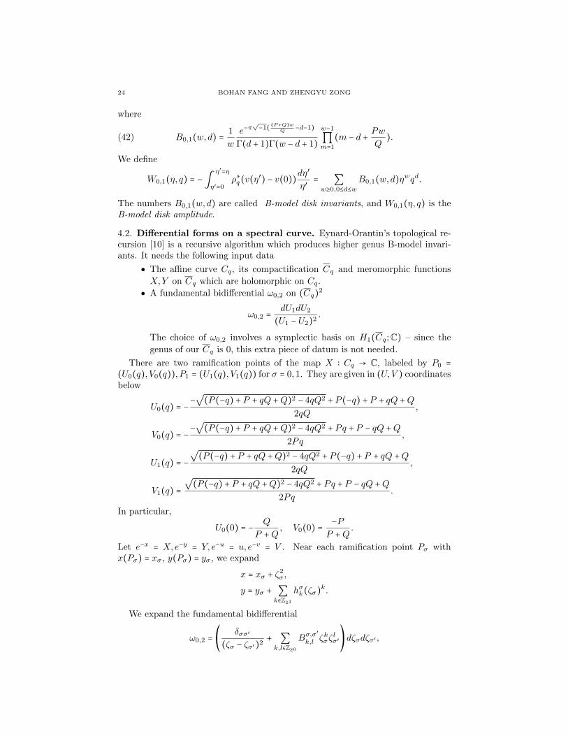
24 BOHAN FANG AND ZHENGYU ZONG
where
B0,1(w,d) =1
w
e−π√−1(
(P+Q)wQ −d−1)
Γ(d + 1)Γ(w − d + 1)
w−1
∏m=1
(m − d +Pw
Q).(42)
We define
W0,1(η, q) = −∫η′=η
η′=0ρ∗q(v(η
′) − v(0))
dη′
η′= ∑w≥0,0≤d≤w
B0,1(w,d)ηwqd.
The numbers B0,1(w,d) are called B-model disk invariants, and W0,1(η, q) is theB-model disk amplitude.
4.2. Differential forms on a spectral curve. Eynard-Orantin’s topological re-cursion [10] is a recursive algorithm which produces higher genus B-model invari-ants. It needs the following input data
The affine curve Cq, its compactification Cq and meromorphic functions
X,Y on Cq which are holomorphic on Cq.
A fundamental bidifferential ω0,2 on (Cq)2
ω0,2 =dU1dU2
(U1 −U2)2.
The choice of ω0,2 involves a symplectic basis on H1(Cq;C) – since the
genus of our Cq is 0, this extra piece of datum is not needed.
There are two ramification points of the map X ∶ Cq → C, labeled by P0 =
(U0(q), V0(q)), P1 = (U1(q), V1(q)) for σ = 0,1. They are given in (U,V ) coordinatesbelow
U0(q) = −−√
(P (−q) + P + qQ +Q)2 − 4qQ2 + P (−q) + P + qQ +Q
2qQ,
V0(q) = −−√
(P (−q) + P + qQ +Q)2 − 4qQ2 + Pq + P − qQ +Q
2Pq,
U1(q) = −
√(P (−q) + P + qQ +Q)2 − 4qQ2 + P (−q) + P + qQ +Q
2qQ,
V1(q) =
√(P (−q) + P + qQ +Q)2 − 4qQ2 + Pq + P − qQ +Q
2Pq.
In particular,
U0(0) = −Q
P +Q, V0(0) =
−P
P +Q.
Let e−x = X,e−y = Y, e−u = u, e−v = V . Near each ramification point Pσ withx(Pσ) = xσ, y(Pσ) = yσ, we expand
x = xσ + ζ2σ,
y = yσ + ∑k∈Z≥1
hσk(ζσ)k.
We expand the fundamental bidifferential
ω0,2 =⎛
⎝
δσσ′
(ζσ − ζσ′)2+ ∑k,l∈Z≥0
Bσ,σ′
k,l ζkσζ
lσ′⎞
⎠dζσdζσ′ ,

TOPOLOGICAL RECURSION FOR TORUS KNOTS 25
and define
Bσ,σ′
k,l =(2k − 1)!!(2l − 1)!!
2k+l+1Bσ,σ
′
k,l ,
hσk = 2(2k − 1)!!hσ2k−1.
We also define the differential of the second kind [10].
θdσ(p) = −(2d − 1)!!2−dResp′→pσB(p, p′)ζ−2d−1σ .
They satisfy and are uniquely characterized by the following properties.
θdσ is a meromorphic 1-form on Cq with a single pole of order 2d+ 2 at Pσ. In local coordinates
θdσ = (−(2d + 1)!!
2dζ2d+2d
+ analytic part in ζσ) .
In the asymptotic expansion we define the formal power series by the asymptoticexpansion
R σσ′ (z) =
√ze−
uσ
z
2√π∫γσe−
xz θ0σ′ .
Here γα is the Lefschetz thimble under the map x, i.e. x(γα) = [xα,∞).For σ = 0,1, define
ξkσ = (−1)k(d
dx)k−1 θ
0σ
dx, k ∈ Z≥1,
θkσ = dξkσ, k ≥ 1, θ0
σ = θ0σ,
θσ(z) =∞
∑k=0
θkσzk, θσ(z) =
∞
∑k=0
θkσzk.
We have the following proposition from [12, Proposition 6.5].
Proposition 4.1.
θσ(z) =1
∑σ′=0
R σσ′ (z)θσ′(z).
Define the following meromorphic form on (Cq)2
C(p1, p2) = −(∂
∂x(p1)−
∂
∂x(p2))(
ω0,2
dx(p1)dx(p2)) (p1, p2)dx(p1)dx(p2).
It is holomorphic on (Cq)2 ∖ Pσ ∶ σ = 0,1. Lemma 6.8 of [12] says
(43) C(p1, p2) =1
2
1
∑σ=0
θ0σ(p1)θ
0σ(p2).
4.3. Higher genus invariants from Eynard-Orantin’s topological recur-sion. For a point p around a ramification point Pα, denote p to be the point suchthat X(p) = X(p), and p ≠ p (i.e. ζσ(p) = −ζσ(p)). The Eynard-Orantin recursionis the following.

26 BOHAN FANG AND ZHENGYU ZONG
Definition 4.2.
ωg,n+1(p1, . . . , pn+1) =1
∑α=0
Resp→Pα− ∫
pξ=p ω0,2(pn+1, p)
2(Φ(p) −Φ(p))⋅ (ωg−1,n+2(p, p, p1, . . . , pn)
+′
∑g1+g2=g,I⊔J=1,...,n
ωg1,∣I ∣(pI , p)ωg2,∣J ∣(pJ , p)),
where Φ = logY dXX
, and ∑′ excludes the case (g1, ∣I ∣) = (0,0), (0,1), (g, n−1), (g, n).
As shown in [10], these ωg,n are symmetric meromorphic forms on (Cq)n, and
they are smooth on (Cq ∖ P0, P1)n. We define the B-model open potentials as
below
W0,2(η1, η2, q) = ∫η1
0∫
η2
0(ρ×2q )
∗C,
Wg,n(η1, . . . , ηn, q) = ∫η1
0. . .∫
ηn(ρ×nq )
∗ωg,n, 2g − 2 + n > 0.
The Eynard-Orantin topological recursion expresses the B-model invariants ωg,nas graph sums [8]. For each decorated graph Γ ∈ Γg,n and p = (p1, . . . , pn) ∈ (Cq)
n,we assign the following weights to each graph component.
Vertex: for a vertex v ∈ V (Γ) labeled by σ = β(v) and g(v), the weight is
(hσ1√−2
)
2−2g−val(v)
⟨ ∏h∈H(v)
τk(h)⟩g(v).
Edge: for an edge e ∈ E(Γ) we assign the weight Bβ(v1(e)),β(v2(e))k,l . In [10],
it is known to be equal to
[zkwl] (1
z +w(δβ(v1(e)),β(v2(e)) − R(z) β(v1(e))
γ R(w)β(v2(e))γ )) .
Dilaton leaf: for a dilaton leaf l ∈ L1(Γ) we assign the weight
(L1)β(l)
k(l)= (−
1√−2
)[zk(l)−1]
1
∑σ=0
hσ1 Rβ(l)σ .
Ordinary leaf: for the j-th ordinary leaf lj we assign the weight
(Lp)β(lj)
k(lj)(lj) = −
1√−2θk(lj)
β(lj)(pj).
We define the ordinary B-model weight of a decorated graph to be
wpB(Γ) =(−1)g(Γ)−1
∏v∈V (Γ)
⎛
⎝
hβ(v)1√−2
⎞
⎠
2−2g−val(v)
⟨ ∏h∈H(v)
τk(h)⟩g(v) ⋅ ∏e∈E(Γ)
Bβ(v1(e)),β(v2(e))k,l
⋅ ∏l∈L1(Γ)
(L1)β(l)
k(l)⋅n
∏j=1
(Lp)β(lj)
k(lj)(lj).
For η = (η1, . . . , ηn), one defines the B-model open leaf weight associated to anordinary leaf lj
(Lηj )β(lj)
k(lj)(lj) = −
1√−2∫
ηj
0ρ∗qθ
kσ.

TOPOLOGICAL RECURSION FOR TORUS KNOTS 27
We define the B-model open weight by substituting the ordinary leaf term by theopen leaf
wηB(Γ) =(−1)g(Γ)−1∏
v∈V (Γ)
⎛
⎝
hβ(v)1√−2
⎞
⎠
2−2g−val(v)
⟨ ∏h∈H(v)
τk(h)⟩g(v) ⋅ ∏e∈E(Γ)
Bβ(v1(e)),β(v2(e))k,l
(44)
⋅ ∏l∈L1(Γ)
(L1)β(l)
k(l)⋅n
∏j=1
(Lη)β(lj)
k(lj)(lj).
Theorem 4.3 (Graph sum formula for ωg,n [8, 9]).
ωg,n(p) = ∑Γ∈Γg,n
wpB(Γ)
Aut(Γ);(45)
∫
η1
0. . .∫
ηn
0(ρ×nq )
∗ωg,n = ∑Γ∈Γg,n
wηB(Γ)
Aut(Γ).
5. Mirror symmetry for open invariants with respect to LP,Q
5.1. Mirror theorem for genus 0 descendants. We follow the notation ofGivental [15]. Define the equivariant small I-function as below
(46) I(z, τ0, τ1) = eτ0v+τ1H
TP,Q
z ∑d≥0
eτ1d∏−1m=−d(
D1
z− d −m)(D2
z− d −m)
∏d−1m=0(
D3
z+ d −m)∏
d−1m=0(
D4
z+ d −m)
.
Here each Di is the equivariant first Chern class of the equivariant line bundleassociated to each toric divisor. The equivariant small J-function is
J(z, τ0, τ1) = eτ0v+τ1H
TP,Q
z (1 +∑d>0
eτ1d(evd1)∗1
z(z − ψ1))
= eτ0v+τ1H
TP,Q
z
1
∑σ=0
⟨φσ
z(z − ψ1)⟩X0,1,de
τ1dφσ.
We quote the famous mirror theorem [13–15, 24, 25] below for X = [OP1(−1) ⊕OP1(−1)]. The mirror map is trivial in this particular situation.
Theorem 5.1 (Givental, Lian-Liu-Yau).
I(z, τ0, τ1) = J(z, τ0, τ1).
In the rest of this paper, we denote the trivial mirror map as below
(47) τ0 = 0, τ1 = log q, τ = τ (q) = (log q)HTP,Q .
For any τ ∈H∗TP,Q
(X;C), the canonical basis φσ(τ ) is decomposed as
φσ(τ ) = Bσ(τ )HTP,Q +Cσ(τ ),
where Bσ(τ ),Cσ(τ ) ∈ STP,Q . We quote a proposition from [12, Section 4.4 andProposition 6.2, ].

28 BOHAN FANG AND ZHENGYU ZONG
Proposition 5.2. We have
hσ12θ0σ = −Bσ(τ (q))∣v=1d
⎛
⎝
q ∂Φ∂q
dx
⎞
⎠+Cσ(τ (q))∣v=1d(
dy
dx) .
5.2. Mirror symmetry for disk invariants. In this section we use the genus 0mirror theorem to compute the descendant part of the disk potential, and identifyit with the non-fractional parts of the B-model disk invariants.
Let f ∈ CJη1, . . . , ηnK. For a fixed integer number Q > 0, we denote
hη1,...,ηn ⋅ f(η1, . . . , ηn) =Q−1
∑k1,...,kn=0
f(ak1η1, . . . , aknηn)
Qn,
where a is a primitive Q-th root of unity. This operation “throws away” all termswith degree not divisible by Q. If f is an actual function analytic at 0, we also usethe same notation.
Recall that in Section 3, we define the A-model disk amplitude as
FX ,LP,Q0,1 (X,τ ) = ∑
µ>0
⟪⟫0,0,µ∣Q=1Xµ.
We have
ι∗0D1 = Qv, ι∗0D2 = P v, ι∗0D3 = −(P +Q)v, ι∗0D4 = 0,
and
(48) ι∗0I(z, t0, t1) = et0z ∑d≥0
et1dSd∏−1m=−d(
Qvz− d −m)(P v
z− d −m)
∏d−1m=0(
−(P+Q)vz
+ d −m)d!.
The pullback along ι0 is
ι∗0J(z, t0, t1) = et0z ∑d≥0
⟨φ0
z(z − ψ1)⟩X0,1,de
t1d.
By the mirror theorem and Equation (48), when τ0 = 0
FX ,LP,Q0,1 (X,τ1) = ∑
µ>0
D(µ)Xµ∑d≥0
edt1⟨φ0
vµ( vµ− ψ1)
⟩X0,1,d
= ∑µ>0
D(µ)Xµ∑d≥0
qd∏−1m=−d(Qµ − d −m)(Pµ − d −m)
∏d−1m=0(−(P +Q)µ + d −m)d!
= ∑µ>0,0≤d≤Qµ
(−1)(Q+P )µ−d−1Xµqd∏Qµ−1m=1 (Pµ − d +m)
d!(Qµ − d)!.
Here we identify eτ1 = q. Comparing with Equation (42), we have the following disktheorem.
Theorem 5.3 (Disk mirror theorem for LP,Q).
FX ,LP,Q0,1 = Q(hη ⋅W0,1)(η, q),
where (hη ⋅W0,1)(η, q) = hη ⋅ (∫η′=ηη′=0 ρ∗q(v(η
′) − v(0))(−dη′
η′)).

TOPOLOGICAL RECURSION FOR TORUS KNOTS 29
5.3. Matching the graphs sums. The localization formula (26) in Section 3, and
Givental’s graph sum formula [16, 17] express FX ,LP,Qg,n as in Equation (29). As a
special case of [12, Theorem 7.1], we know under the trivial mirror map (47)
(49) R σσ′ (z)∣τ=(log q)HTP,Q ,Q=1,v=1 = R
σσ′ (−z).
Also from [12, Section 4.4 and Lemma 4.3] and the fact hσ1 =√
2/d2xdy2 by direct
calculation, we have
hσ1√−2
=
√1
∆σ(τ )∣v=1.
Immediately from these facts and the graph sum formulae (45) and (23), theweights in the graph sum match except for the open leafs. We will compare themin the next section.
5.4. Matching open leaves. We define
Uz(τ,X) =1
∑σ′=0
ξσ′
(z,X)S(1, φσ′)∣Q=1.
By Equation (27),
FX ,LP,Q0,1 (τ ,X) = [z−2
]1
∑σ′=0
ξσ′
(z,X)S(1, φσ′)∣Q=1,
(Xd
dX)2FX ,LP,Q0,1 (τ ,X) = [z0
]1
∑σ′=0
ξσ′
(z,X)S(1, φσ′)∣Q=1v2.
Since FX ,LP,Q0,1 = Q(hη ⋅W0,1)(η, q) (Theorem 5.3), as power series in X,
[z0](v2U(z)(τ,X)) = −(
ηd
Qdη)(hη ⋅ ρ
∗q)(v)
(v2U(z)(τ,X))≥−1
= − ∑n≥−1
(z
v)n(ηd
Qdη)n+1
(hη ⋅ ρ∗q)(v).(50)
Here ()≥a truncates the z-series, keeping terms whose power is greater or equal thana. We usually denote ()≥0 by ()+.
If we write the canonical basis by flat basis
φσ(τ (q)) = Bσ(q)HTP,Q + Cσ(q)1,
then1
∑σ′=0
ξσ′
(z,X)S(φσ(τ (q)), φσ′)∣Q=1= zBσ(q)
∂U
∂τ1+ Cσ(q)U.
Here we use the fact that S(HLP,Q , φσ′) = z∂S(1,φσ′)
∂τ1. From Proposition 5.2,
−θ0σ√−2
= −Bσ(q)∣v=1d(q ∂Φ∂q
dx) + Cσ(q)∣v=1d(
dy
dx)
=1
Q(−Bσ(q)∣v=1d(q
∂v
∂q) + Cσ(q)∣v=1d(
dv
dx)) .(51)
By Equation (50) and (51), under the open-closed mirror map

30 BOHAN FANG AND ZHENGYU ZONG
hη ⋅ ∫η
0
ρ∗qθ0σ
√−2
= −1
Q(−Bσ(q)∣v=1(q
∂(hη ⋅ ρ∗qv)
∂q) + Cσ(q)∣v=1
d(hη ⋅ ρ∗qv)
dx)
= −1
Q(−Bσ(q)∣v=1
∂(hη ⋅ ρ∗qv)
∂τ1− Cσ(q)∣v=1(
ηd
Qdη)(hη ⋅ ρ
∗qv)))
= −1
Q(Bσ(q)[z
−1]∂U(z)(τ,X)
∂τ1+ Cσ(q)[z
0]U(z)(τ,X))
v=1
,
Therefore
hη ⋅ ∫η
0
ρ∗q θσ(z)√−2
= ∑a≥0
za(Xd
dX)a(hη ⋅ ∫
η
0
ρ∗qθ0σ
√−2
)(52)
= −1
Q(+Bσ(q)z
∂U≥−1
∂τ1+ Cσ(q)U≥0)
= −1
Q(
1
∑σ′=0
ξσ′
(z,X)S(φσ(τ (q)), φσ′)∣Q=1)
+
.
Theorem 5.4 (BEM-DSV conjecture for annulus invariants).
FX ,LP,Q0,2 (X1,X2,τ )∣τ=τ(q) = −Q
2hη1,η2 ⋅W0,2(η1, η2, q).
Proof.
hη1,η2 ⋅ ((η1∂
Q∂η1+ η2
∂
Q∂η2)W0,2(q;η1, η2))
=hη1,η2 ⋅ (∫
η1
0∫
η2
0(ρ×2q )
∗C) =1
2
1
∑σ=0
(hη1 ⋅ ∫
η1
0(ρq)
∗θ0σ)(hη2 ⋅ ∫
η2
0(ρq)
∗θ0σ)
= −1
Q2[z−2
1 z−22 ]
1
∑σ,σ′,σ′′=0
ξσ′′
(z1,X1)ξσ′(z2,X2)S(φσ(τ ), φσ′)∣τ=τ(q),Q=1
S(φσ(τ ), φσ′′)∣τ=τ(q),Q=1
= −1
Q2[z−2
1 z−22 ](z1 + z2)
1
∑σ′,σ′′=0
V (φσ′ , φσ′′)∣τ=τ(q),Q=1ξσ
′
(z1,X1)ξσ′′
(z2,X2)
= −1
Q2[z−1
1 z−12 ](X1
∂
∂X1+X2
∂
∂X2)
1
∑σ′,σ′′=0
V (φσ′ , φσ′′)∣τ=τ(q),Q=1ξσ
′
(z1,X1)ξσ′′
(z2,X2)
= −1
Q2(X1
∂
∂X1+X2
∂
∂X2)FX ,LP,Q0,2 (X1,X2,τ ).
where the second equality follows from Equation (43), the fourth equality followsfrom Equation (52), the fifth equality is WDVV (Equation (20)), and the lastequality follows from (28).
Theorem 5.5 (BEM-DSM conjecture for 2g − 2 + n > 0).
FX ,LP,Qg,n (X1, . . . ,Xn,τ )∣τ=τ(q) = (−1)g−1+nQn(h ⋅Wg,n)(η1, . . . , ηn, q).
Proof. As shown in Section 5.3, other than open leaf terms, the A-model graphweights match B-model graph weights under the trivial mirror map (47) and after

TOPOLOGICAL RECURSION FOR TORUS KNOTS 31
setting the A-model equivariant parameter v = 1. By Equation (52), the A-modelopen leaf is
(LX)σk ∣v=1 = −Q[zk]
1√−2
h ⋅ (∫η
0
1
∑σ′=0
(R σσ′ (−z)) ∣τ=τ(q),Q=1,v=1ρ
∗q θσ′(z)) ,
while the B-model open leaf is
(Lη)σk = [zk]
1√−2∫
η
0
1
∑σ′=0
R σσ′ (−z)∣τ=τ(q),Q=1,v=1ρ
∗q θσ′(z).
So
(LX)σk ∣v=1 = −Qh ⋅ (Lη)σk .
Therefore, for any decorated stable graph Γ, since A-model open potential does notdepend on the equivariant parameter, i.e. a scalar of cohomological degree 0 in theequivariant cohomology, then
wXA (Γ) = wXA (Γ)∣v=1 = (−1)g−1+nQn(h ⋅wηB(Γ)).
The factor (−1)g−1 comes from the B-model graph sum formula (44), while thefactor (−Q)n comes from the factor −Q for open leaves.
References
[1] M. Aganagic and C. Vafa, Mirror symmetry, D-branes and counting holomorphic discs.arXiv:hep-th/0012041.
[2] M. Aganagic, A. Klemm, and C. Vafa, Disk instantons, mirror symmetry and the dualityweb, Z. Naturforsch. A 57 (2002), no. 1-2, 1–28.
[3] V. Bouchard, A. Klemm, M. Marino, and S. Pasquetti, Remodeling the B-model, Comm.
Math. Phys. 287 (2009), no. 1, 117–178.[4] A. Brini, B. Eynard, and M. Marino, Torus knots and mirror symmetry, Ann. Henri Poincare
13 (2012), no. 8, 1873–1910.
[5] D. Cox and S. Katz, Mirror symmetry and algebraic geometry, Math. Surveys and mono-graphs 68, American Math. Soc., Providence, RI, 1999.
[6] D.-E. Diaconescu, V. Shende, and C. Vafa, Large N duality, Lagrangian cycles, and algebraic
knots, Comm. Math. Phys. 319 (2013), no. 3, 813-863.[7] R. Gopakumar and C. Vafa, On the gauge theory/geometry correspondence, Adv. Theor.
Math. Phys. 3 (1999), no. 5, 1415-1443.[8] P. Dunin-Barkowski, N. Orantin, S. Shadrin, and L. Spitz, Identification of the Givental
formula with the spectral curve topological recursion procedure, Comm. Math. Phys. 328
(2014), no. 2, 669–700.[9] B. Eynard, Intersection number of spectral curves. arXiv:1104.0176.
[10] B. Eynard and N. Orantin, Invariants of algebraic curves and topological expansion, Commun.
Number Theory Phys. 1 (2007), no. 2, 347–452.[11] B. Eynard and N. Orantin, Computation of open Gromov-Witten invariants for toric Calabi-
Yau 3-folds by topological recursion, a proof of the BKMP conjecture, Comm. Math. Phys.
337 (2015), no. 2, 483–567.[12] B. Fang, C.-C. M. Liu, and Z. Zong, On the remodeling conjecture for toric Calabi-Yau
3-orbifolds. arXiv:1604.07123.
[13] A. Givental, Equivariant Gromov-Witten invariants, Internat. Math. Res. Notices 13 (1996),613–663.
[14] , A mirror theorem for toric complete intersections, Topological field theory, primitiveforms and related topics (Kyoto, 1996), Progr. Math., vol. 160, Birkhauser Boston, Boston,
MA, 1998, pp. 141–175.
[15] , Elliptic Gromov-Witten invariants and the generalized mirror conjecture, Integrablesystems and algebraic geometry (Kobe/Kyoto, 1997), World Sci. Publ., River Edge, NJ, 1998,pp. 107–155.

32 BOHAN FANG AND ZHENGYU ZONG
[16] , Semisimple Frobenius structures at higher genus, Internat. Math. Res. Notices 23
(2001), 1265–1286.
[17] , Gromov-Witten invariants and quantization of quadratic hamiltonians, Mosc. Math.J. 1 (2001), no. 4, 551–568.
[18] J. Gu, H. Jockers, A. Klemm, and M. Soroush, Knot invariants from topological recursion
on augmentation varieties, Comm. Math. Phys. 336 (2015), no. 2, 987–1051.[19] S. Katz and C.-C. M. Liu, Enumerative geometry of stable maps with Lagrangian boundary
conditions and multiple covers of the disc, Adv. Theor. Math. Phys. 5 (2001), no. 1, 1–49.
[20] S. Koshkin, Conormal bundles to knots and the Gopakumar-Vafa conjecture, Adv. Theor.Math. Phys. 11 (2007), no. 4, 591–634.
[21] J. M. F. Labastida, M. Marino, and C. Vafa, Knots, links and branes at large N , J. High
Energy Phys. 11 (2000), Paper 7, 42.[22] J. Li, C.-C. Liu, K. Liu, and J. Zhou, A mathematical theory of the topological vertex, Geom.
Topol. 13 (2009), no. 1, 527–621.[23] Y.-P. Lee and R. Pandharipande, Frobenius manifolds, Gromov-Witten theory and virasoro
constraints, Preprint.
[24] B. Lian, K. Liu, and S.-T. Yau, Mirror principle I, Asian J. Math. 1 (1997), no. 4, 729–763.[25] , Mirror principle II, Asian J. Math. 3 (1999), no. 1, 109–146.
[26] C.-C. M. Liu, Moduli of J-holomorphic curves with Lagrangian boundary conditions and open
Gromov-Witten invariants for an S1-equivariant pair. arXiv:math/0210257.[27] C.-C. M. Liu, K. Liu, and J. Zhou, A proof of a conjecture of Mario-Vafa on Hodge integrals,
J. Differential Geom. 65 (2003), no. 2, 289–340.
[28] M. Mahowald, Knots and Gamma classes in open topological string theory, Ph.D. Thesis,Northwestern University, 2016.
[29] M. Marino, Chern-Simons theory and topological strings, Rev. Modern Phys. 77 (2005), no. 2,
675–720.[30] , Chern-Simons theory, the 1/N expansion, and string theory. arXiv:1001.2542.
[31] M. Marino and C. Vafa, Framed knots at large N, Orbifolds in mathematics and physics(Madison, WI, 2001), Contemp. Math., vol. 310, Amer. Math. Soc., Providence, RI, 2002,
pp. 185-204.
[32] D. McDuff and D. Salamon, Introduction to symplectic topology, Second, Oxford Mathemat-ical Monographs, The Clarendon Press Oxford University Press, New York, 1998.
[33] A. Okounkov and R. Pandharipande, Hodge integrals and invariants of the unknot, Geom.
Topol. 8 (2004), 675–699.[34] H. Ooguri and C. Vafa, Knot invariants and topological strings, Nuclear Phys. B 577 (2000),
no. 3, 419–438.
[35] C. H. Taubes, Lagrangians for the Gopakumar-Vafa conjecture, Adv. Theor. Math. Phys. 1(2001), 139–163.
[36] E. Witten, Quantum field theory and the Jones polynomial, Comm. Math. Phys. 121 (1989),no. 3, 351-399.
[37] , Chern-Simons gauge theory as a string theory, The Floer memorial volume, Progr.
Math., vol. 133, Birkhauser, Basel, 1995, pp. 637-678.
Bohan Fang, Beijing International Center for Mathematical Research, Peking Uni-versity, 5 Yiheyuan Road, Beijing 100871, China
E-mail address: [email protected]
Zhengyu Zong, Yau Mathematical Sciences Center, Tsinghua University, Jin ChunYuan West Building, Tsinghua University, Haidian District, Beijing 100084, China
E-mail address: [email protected]

![CS240 recursion Fall 2014 n -zh n] 1. See “recursion” Mike ... · CS240 Fall 2014 Mike Lam, Professor Recursion recursion n. [ri-kur-zhuh n] 1. See “recursion”](https://static.fdocuments.us/doc/165x107/5e67d0b07bf39a6a43705e7c/cs240-recursion-fall-2014-n-zh-n-1-see-aoerecursiona-mike-cs240-fall-2014.jpg)


![Topological Quantum Field Theories in Topological Recursionof some Topological Recursion due to results in Cohomological Field Theory [6]. We consider a graphical approach to both](https://static.fdocuments.us/doc/165x107/5edd3c00ad6a402d6668414b/topological-quantum-field-theories-in-topological-recursion-of-some-topological.jpg)