Topological recursion and geometry - arXiv · Topological recursion and geometry Ga¨etan Borot *...

Topological recursion and geometry

Gaetan Borot*

Mini-course, Institut Mathematique de Toulouse, France.

May 12th, 2017

Contents

1 Quantum Airy structures 3

1.1 First principles . . . . . . . . . . . . . . . . . . . . . . . . . . . . . 3

1.2 Partition function and topological recursion . . . . . . . . . . . 6

1.3 The structure of TR . . . . . . . . . . . . . . . . . . . . . . . . . . 10

1.4 A one-dimensional example . . . . . . . . . . . . . . . . . . . . . 12

1.5 Operations on quantum Airy structures . . . . . . . . . . . . . . 13

1.6 Bonus: from classical to quantum Airy structures . . . . . . . . 15

2 Two-dimensional topological quantum field theories 18

2.1 Definitions . . . . . . . . . . . . . . . . . . . . . . . . . . . . . . . 18

2.2 Correspondence with Frobenius algebras . . . . . . . . . . . . . 19

2.3 Computing the tqft amplitudes . . . . . . . . . . . . . . . . . . 20

3 Intersection theory on the moduli space of curves 22

3.1 A quantum Airy structure on the loop space . . . . . . . . . . . 22

3.2 Witten-Kontsevich partition function . . . . . . . . . . . . . . . . 24

4 Cohomological field theories 27

4.1 Definition . . . . . . . . . . . . . . . . . . . . . . . . . . . . . . . 27

4.2 Two examples. . . . . . . . . . . . . . . . . . . . . . . . . . . . . . 29

4.3 Motivating example: quantum cohomology and Gromov-Wittentheory . . . . . . . . . . . . . . . . . . . . . . . . . . . . . . . . . . 30

4.4 Givental group action . . . . . . . . . . . . . . . . . . . . . . . . 31

4.5 Semi-simple cohomological field theories . . . . . . . . . . . . . 33

5 Volumes of the moduli space of curves 35

5.1 Teichmuller space of bordered surfaces . . . . . . . . . . . . . . 35

5.2 Mirzakhani’s recursion . . . . . . . . . . . . . . . . . . . . . . . . 37

5.3 Sketch of the proof of Theorem 5.1 . . . . . . . . . . . . . . . . . 40

References 47

*Max-Planck Institut for Mathematics: [email protected]

1

arX

iv:1

705.

0998

6v1

[m

ath-

ph]

28

May

201

7

mailto:Max-Planck Institut for Mathematics: [email protected]

Contents

These are lecture notes for a 4h mini-course held in Toulouse, May 9-12th,at the thematic school on

Quantum topology and geometry

I thank Francesco Costantino and Thomas Fiedler for organization of thisevent, the audience and especially Rinat Kashaev and Gregor Masbaum forquestions and remarks which improved the lectures.

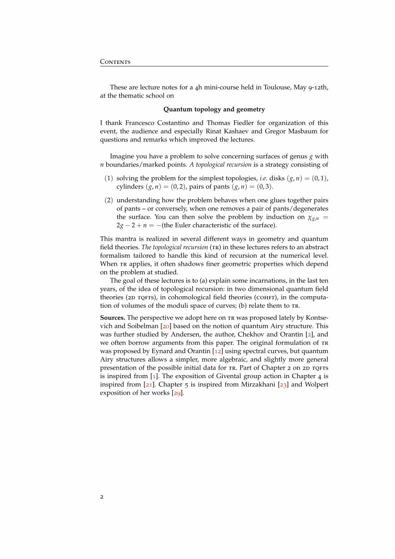
Imagine you have a problem to solve concerning surfaces of genus g withn boundaries/marked points. A topological recursion is a strategy consisting of

(1) solving the problem for the simplest topologies, i.e. disks (g, n) = (0, 1),cylinders (g, n) = (0, 2), pairs of pants (g, n) = (0, 3).

(2) understanding how the problem behaves when one glues together pairsof pants – or conversely, when one removes a pair of pants/degeneratesthe surface. You can then solve the problem by induction on χg,n =2g− 2 + n = −(the Euler characteristic of the surface).

This mantra is realized in several different ways in geometry and quantumfield theories. The topological recursion (tr) in these lectures refers to an abstractformalism tailored to handle this kind of recursion at the numerical level.When tr applies, it often shadows finer geometric properties which dependon the problem at studied.

The goal of these lectures is to (a) explain some incarnations, in the last tenyears, of the idea of topological recursion: in two dimensional quantum fieldtheories (2d tqfts), in cohomological field theories (cohft), in the computa-tion of volumes of the moduli space of curves; (b) relate them to tr.

Sources. The perspective we adopt here on tr was proposed lately by Kontse-vich and Soibelman [20] based on the notion of quantum Airy structure. Thiswas further studied by Andersen, the author, Chekhov and Orantin [2], andwe often borrow arguments from this paper. The original formulation of tr

was proposed by Eynard and Orantin [12] using spectral curves, but quantumAiry structures allows a simpler, more algebraic, and slightly more generalpresentation of the possible initial data for tr. Part of Chapter 2 on 2d tqftsis inspired from [1]. The exposition of Givental group action in Chapter 4 isinspired from [21]. Chapter 5 is inspired from Mirzakhani [23] and Wolpertexposition of her works [29].

2

Lecture 1 (1h)May 9th, 2017

1 Quantum Airy structures

1.1 First principles

The initial data for tr is a “quantum Airy structure”. This notion was intro-duced by Kontsevich and Soibelman in [20]. Let V be a vector space over afield K of characteristic 0. Let (ei)i∈I be a basis of V, and (xi)i∈I the corre-sponding basis of linear coordinates. h denotes a formal parameter. If V isinfinite dimensional, we may have to add assumptions (filtration, completion,convergence) so that all expressions we write make sense. We will overlookthis issue, and in the examples of quantum Airy structures with dim V = ∞we meet, it is possible to check that seemingly infinite sums we are going towrite actually contain only finitely many non-zero terms.

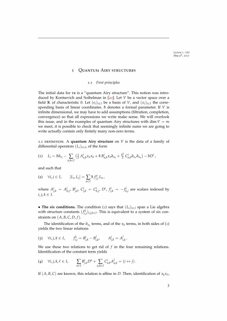
1.1 definition. A quantum Airy structure on V is the data of a family ofdifferential operators (Li)i∈I , of the form

(1) Li = h∂xi − ∑a,b∈I

( 12 Ai

a,bxaxb + h Bia,bxa∂xb +

h2

2 Cia,b∂xa ∂xb

)− hDi ,

and such that

(2) ∀i, j ∈ I, [Li, Lj] = ∑a∈I

h f ai,j La ,

where Aij,k = Ai

k,j, Bij,k, Ci

j,k = Cik,j, Di, f i

j,k = − f ik,j are scalars indexed by

i, j, k ∈ I.

• The six conditions. The condition (2) says that (Li)i∈I span a Lie algebrawith structure constants ( f k

i,j)i,j,k∈I . This is equivalent to a system of six con-straints on (A, B, C, D, f ).

The identification of the ∂xk terms, and of the xk terms, in both sides of (2)yields the two linear relations

(3) ∀i, j, k ∈ I, f ki,j = Bi

j,k − Bji,k, Ai

j,k = Aji,k .

We use these two relations to get rid of f in the four remaining relations.Identification of the constant term yields

(4) ∀i, j, k, ` ∈ I, ∑a∈I

Bij,aDa + ∑

a,b∈ICi

a,b Aja,b = (i↔ j) .

If (A, B, C) are known, this relation is affine in D. Then, identification of xkx`,

3

1. Quantum Airy structures

xk∂x` and ∂xk ∂x` yields

(5) ∀i, j, k, ` ∈ I,

∑a∈I Bij,a Aa

k,` + Bik,a Aj

a,` + Bi`,a Aj

a,k = (i↔ j)

∑a∈I Bij,aBa

k,` + Bik,aBj

a,` + Ci`,a Aj

a,k = (i↔ j)∑a∈I Bi

j,aCak,` + Ci

k,aBia,` + Ci

`,aBia,` = (i↔ j)

.

These three quadratic relations have the same index structure. In fact, theyform a system of three coupled IHX-type relations (Figure 1). The relationinvolving D is depicted in Figure 2.

+ +

+ +

+ +

1

23 1 2

3

1

2

3

1 2

3

1 2

3

1

23

1

2

3

1

2

3

1

2 3

1

1

1

1

1

23

i

j

k

`

i

j

k

`

i

j

k

`

i

j

k

`

i

j

k

`

i

j

k

`

i

j

k

`

i

j

k

`

i

j

k

`

Figure 1: A red dot is replaced by a B, a green dot by a C, a blue dot byan A. The labels 1, 2, 3 specify the ordering of indices at a B-vertex, namelyBi1

i2,i3, and 1 at C-vertex specifies the first index Ci1∗∗. Such an ordering is not

necessary at an A-vertex as A is fully symmetric. The dashed line carries anindex a ∈ I which is summed over. Equation (5) says that each of the threelines is symmetric under permutation of i and j.

• Counting. If dim V = d, let us count the number of unknowns and indepen-dent conditions determining a quantum Airy structure. As (3) fixes f in terms

4

1.1. First principles

+

1 2

3i

12

j

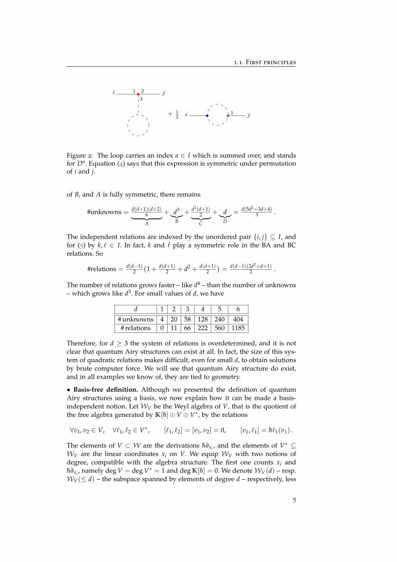
i j1

Figure 2: The loop carries an index a ∈ I which is summed over, and standsfor Da. Equation (4) says that this expression is symmetric under permutationof i and j.

of B, and A is fully symmetric, there remains

#unknowns = d(d+1)(d+2)6︸︷︷︸A

+ d3︸︷︷︸

B

+ d2(d+1)2︸︷︷︸C

+ d︸︷︷︸D

= d(5d2+3d+4)3 .

The independent relations are indexed by the unordered pair i, j ⊆ I, andfor (5) by k, ` ∈ I. In fact, k and ` play a symmetric role in the BA and BCrelations. So

#relations = d(d−1)2(1 + d(d+1)

2 + d2 + d(d+1)2)= d(d−1)(2d2+d+1)

2 .

The number of relations grows faster – like d4 – than the number of unknowns– which grows like d3. For small values of d, we have

d 1 2 3 4 5 6

# unknowns 4 20 58 128 240 404# relations 0 11 66 222 560 1185

Therefore, for d ≥ 3 the system of relations is overdetermined, and it is notclear that quantum Airy structures can exist at all. In fact, the size of this sys-tem of quadratic relations makes difficult, even for small d, to obtain solutionsby brute computer force. We will see that quantum Airy structure do exist,and in all examples we know of, they are tied to geometry.

• Basis-free definition. Although we presented the definition of quantumAiry structures using a basis, we now explain how it can be made a basis-independent notion. Let WV be the Weyl algebra of V, that is the quotient ofthe free algebra generated by K[h]⊕V ⊕V∗, by the relations

∀v1, v2 ∈ V, ∀`1, `2 ∈ V∗, [`1, `2] = [v1, v2] = 0, [v1, `1] = h`1(v1) .

The elements of V ⊂ W are the derivations h∂xi , and the elements of V∗ ⊆WV are the linear coordinates xi on V. We equip WV with two notions ofdegree, compatible with the algebra structure. The first one counts xi andh∂xi , namely deg V = deg V∗ = 1 and deg K[h] = 0. We denoteWV(d) – resp.WV(≤ d) – the subspace spanned by elements of degree d – respectively, less

5


or equal to d. The second one is the usual h-degree on K[h], supplemented bythe assignments deghV = degh V∗ = 0. In other words, hkx`∂m has h-degree(k−m). This convention may seem unnatural, but it is convenient for the nextdefinition.

We remark that WV(≤ 2) is a Lie algebra, while WV(≤ d) is not d ≥ 3as can be seen from degree counting. This justifies considering operators ofdegree at most 2. We denote πd and π≤d the projection onto the subspacesWV(d) andWV(≤ d).

1.2 definition. A quantum Airy structure on V is the data of a Lie algebrastructure on V and a homomorphism of Lie algebras L : V →WV(≤ 2) suchthat

• Im(π1 L) = V ⊆ WV(1), and π1 L induces an isomorphism ϕ : V →V ⊆ WV(1).

• for d ∈ 0, 1, 2, we have degh(πd L) = δd,0.

As WV(2) =(Sym2(V∗ ⊕ V)

)[h] and taking into account the h-degree

condition, π2 L decomposes into three tensors. Turning a V∗ in the target toa V in the source, they can be arranged as

A ∈ HomK(V⊗3, K), B ∈ HomK(V⊗2, V), C ∈ HomK(V, V⊗2) .

Besides, h−1(π0 L) gives

D ∈ HomK(V, K) .

The conditions (3)-(4)-(5) on (A, B, C, D) expressing that L is a Lie algebramorphism can written solely in terms of composition of these morphisms. Infact, they would make sense in the more general context of V being an objectin a symmetric monoidal category – here we worked with the category VectK

of finite-dimensional K-vector fields.The relation between Definitions 1.1 and 1.2 is as follows. If (ei)i∈I is a basis

of V, we should consider it as a basis of V ⊆ WV and then Li = L(ϕ−1(ei))for all i ∈ I.

1.2 Partition function and topological recursion

Taking a quantum Airy structure L as input, we can get a function on V whichis simultaneously annihilated by the differential operators given by L. Moreprecisely, the output F will belong to the space

(6) EV = h−1 Sym>0V∗[[h]] .

We equip EV with the Euler degree, defined through degχ hg−1 SymnV∗ =χg,n = 2g− 2 + n. Elements F ∈ EV can be decomposed

F = ∑g≥0

∑n≥1

hg−1

n!Fg,n, Fg,n ∈ Symn(V∗) .

6

1.2. Partition function and topological recursion

We make a small abuse of vocabulary by saying that the Euler degree of Fg,nis χg,n, and we declare that the Euler degree of a product is the sum of theEuler degrees.

1.3 theorem. [20, 2] If L is a quantum Airy structure on V, there exists a uniqueF ∈ EV such that F0,1 = 0, F0,2 = 0, and for all v ∈ V we have

L(v) exp(F) = 0 .

.

To fix the vocabulary, we will call Fg,n the tr amplitudes, F the “free en-ergy”, and Z = exp(F) the “partition function”.

• Proof of uniqueness. For convenience, we are going to use a basis of lin-ear coordinates (xi)i∈I as in Definition 1.1. We also agree that indices a, b, . . .should be summed over the set I, while indices i, j, k, . . . are fixed. If we de-compose

F = ∑g≥0

hg−1 Fg ,

we find that the coefficient of hg in exp(−F)Li exp(F) is

∂xi Fg = δg,012 Ai

a,bxaxb + Bia,bxa∂xb Fg +

12 Ci

a,b

(∂xa ∂xb Fg−1 + ∑

g1+g2=g∂xa Fg1 ∂xb Fg2

)

+δg,1Di .

Let us decompose further

Fg = ∑n≥1

∑i1,...,in∈I

Fg,n[i1, . . . , in]xi1 · · · xin

n!.

Now, for n ≥ 1 we fix an unordered (n− 1)-uple of indices i2, . . . , in ∈ I andcollect the coefficient of the monomial

xi2 ···xin(n−1)! in this equation. Taking into

account the fact that i2, . . . , in are unordered and Fg,n are symmetric, we get

Fg,n[i, i2, . . . , in]

= δg,0δn,3 Aii2,i3 + δg,1δn,1Di +

n

∑m=2

Biim ,a Fg,n−1[a, i2, . . . , im, . . . , in]

+ 12 Ci

a,b

(Fg−1,n+1[a, b, i2, . . . , in] + ∑

g1+g2=gJ1∪J2=i2,...,in

Fg1,1+|J1|[a, J1]Fg2,1+|J2|[b, J2]

).

(7)

As F0,1 and F0,2 are required to vanish, all possibly non-zero Fg,n have Eulerdegree χg,n > 0. According to (7), the cases χg,n = 1 correspond to

(8) F0,3[i, i2, i3] = Aii2,i3 , F1,1[i] = Di ,

7


and for χg,n ≥ 2, we have

Fg,n[i, i2, . . . , in]

=n

∑m=2

Biim ,a Fg,n−1[a, i2, . . . , im, . . . , in]

+ 12 Ci

a,b

(Fg−1,n+1[a, b, i2, . . . , in] + ∑

g1+g2=gJ1∪J2=i2,...,in

Fg1,1+|J1|[a, J1]Fg2,1+|J2|[b, J2]

),

(9)

where we observe that the Euler degree of the right-hand side is χg,n − 1.Therefore, (9) is a recursion on χg,n which has at most one solution.

• Proof of existence. We now have to justify the existence of Fg,n ∈ Symn(V∗)satisfying (8)-(9), the non obvious part being the symmetry. A general holo-nomicity argument proving existence was given in [20]. Here we follow thepedestrian way of [2]. First of all, (8) defines a symmetric F0,3 because A isfully symmetric in a quantum Airy structure. Then, we would like to take(9) as recursive definition of Fg,n. This only makes sense if we can prove ateach recursion step that, despite the fact that i does not play the same role asi2, . . . , in in (9), the result of the sum in the right-hand side is still symmetricwhen i is permuted with one of the im. Note that the i2, . . . , in do play a sym-metric role, so it is enough to prove invariance under permutation of i and i2.Let us examine the two cases where χg,n = 2, that is (g, n) = (0, 4) and (2, 1).We would like to define

F0,4[i, i2, i3, i4] = Bii2,aF0,3[a, i3, i4] + Bi

i3,aF0,3[a, i2, i4] + Bii4,aF0,3[a, i2, i3] .

Using F0,3[i, j, k] = Aij,k which is fully symmetric, this also reads

F0,4[i, i2, i3, i4] = Bii2,a Aa

i3,i4 + Bii3,a Ai2

a,i4+ Bi

i4,a Ai2a,i3

.

We recognize the left-hand side of the first relation in (5), therefore it is invari-ant if we exchange i and i2. We also would like to define

F2,1[i, i2] = Bii2,aDa + 1

2 Cia,bF0,3[a, b, i2] = Bi

i2,aDa + 12 Ci

a,b Ai2a,b .

We recognize the left-hand side of the D relation (4), therefore it is invariantif we exchange i and i2. We see that the conditions imposed on (A, B, C, D) bythe characterization of quantum Airy structures are essential in proving thesymmetry of Fg,n.

Now we examine the general case. Take (g, n) such that χg,n > 2, andassume we have proved full symmetry of Fg′ ,n′ for all χg′ ,n′ < χg,n. Let K =

8

1.2. Partition function and topological recursion

i3, . . . , in. Let us define Fg,n[i, j, K] by applying (9) with first index i.

Fg,n[i, j, K] = Bij,aFg,n−1[a, K] + ∑

k∈KBi

k,aFg,n−1[a, j, K(k)] + 12 Ci

a,bFg−1,n+1[a, b, j, K]

+ ∑h′+h′′=gK′∪K′′=K

Cia,bFh′ ,2+|K′ |[a, j, K′]Fh′′ ,1+|K′′ |[b, K′′] .

The resulting terms are in the range of the induction hypothesis, thus fullysymmetric under permutation of (j, i3, . . . , in). We use again (9) with first indexj, except for the term involving Bi

j,aFg,n−1[a, K], for which we rather use (9)

with first index a. Denote K(k) := K \ k and K(k,`) := K \ k, `. We alsoimplicitly use the full symmetry of A and the symmetry of C in its two lowerindices. The result is

Fg,n[i, j, K]

= Bij,a

∑k∈K

Bak,bFg,n−2[b, K(k)] + 1

2 Cab,cFg−1,n[b, c, K] + ∑

h′+h′′=gK′∪K′′=K

12 Ca

b,cFh′ ,1+|K′ |[b, K′]Fh′′ ,1+|K′′ |[c, K′′]

+ ∑k∈K

Bik,a

Bj

a,bFg,n−2[b, K(k)] + ∑`∈K(k)

Bj`,bFg,n−2[b, a, K(k,`)] + 1

2 Cjb,cFg−1,n[b, c, a, K(k)]

+ ∑h′+h′′=g

K′∪K′′=K(k)

12 Fh′ ,2+|K′ |[b, a, K′]Fh′′ ,1+|K′′ |[c, K′′]

+ 12 Ci

a,b

Bj

a,cFg−1,n[b, c, K] + Bjb,cFg−1,n[a, c, K]

+ ∑k∈K

Bjk,cFg−1,n[b, c, a, K(k)] + 1

2 Cjc,dFg−2,n+2[c, d, a, b, K]

+ ∑h′+h′′=g−1K′∪K′′=K

Cjc,dFh′ ,3+|K′ |[a, b, c, K′]Fh′′ ,1+|K′′ |[d, K′′] + Cj

c,dFh′ ,2+|K′ |[a, c, K′]Fh′′ ,2+|K′′ |[b, d, K′′]

+ ∑h′+h′′=gK′∪K′′=K

Cia,bFh′′ ,1+|K′′ |[b, K′′]

Bj

a,cFh′ ,1+|K′ |[c, K′] + ∑k∈K′

Bjk,cFh′ ,1+|K′ |[c, a, K(k)]

+ 12 Cj

c,dFh′−1,3+|K′ |[c, d, a, K′] + ∑s+s′=h′L∪L′=K′

Cjc,dFs,2+|L|[a, c, L]Fs′ ,1+|L′ |[d, L′] + δh′ ,0δ|K′ |,1 Aj

a,k′

.

9


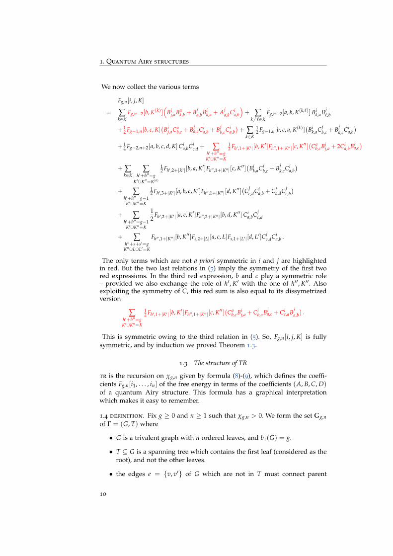
We now collect the various terms

Fg,n[i, j, K]

= ∑k∈K

Fg,n−2[b, K(k)](

Bij,aBa

k,b + Bja,bBi

k,a + Aja,kCi

a,b

)+ ∑

k 6=`∈KFg,n−2[a, b, K(k,`)] Bi

k,aBj`,b

+ 12 Fg−1,n[b, c, K]

(Bi

j,aCab,c + Bj

a,cCia,b + Bj

b,cCia,b)+ ∑

k∈K

12 Fg−1,n[b, c, a, K(k)]

(Bi

k,aCjb,c + Bj

k,cCia,b)

+ 14 Fg−2,n+2[a, b, c, d, K]Ci

a,bCjc,d + ∑

h′+h′′=gK′∪K′′=K

12 Fh′ ,1+|K′ |[b, K′]Fh′′ ,1+|K′′ |[c, K′′]

(Ca

b,cBij,a + 2Ci

a,bBja,c)

+ ∑k∈K

∑h′+h′′=g

K′∪K′′=K(k)

12 Fh′ ,2+|K′ |[b, a, K′]Fh′′ ,1+|K′′ |[c, K′′]

(Bi

k,aCjb,c + Bj

k,cCia,b)

+ ∑h′+h′′=g−1K′∪K′′=K

12 Fh′ ,3+|K′ |[a, b, c, K′]Fh′′ ,1+|K′′ |[d, K′′]

(Cj

c,dCia,b + Ci

a,dCjc,b)

+ ∑h′+h′′=g−1K′∪K′′=K

12

Fh′ ,2+|K′ |[a, c, K′]Fh′′ ,2+|K′′ |[b, d, K′′]Cia,bCj

c,d

+ ∑h′′+s+s′=g

K′′∪L∪L′=K

Fh′′ ,1+|K′′ |[b, K′′]Fs,2+|L|[a, c, L]Fs,1+|L′ |[d, L′]Cjc,dCi

a,b .

The only terms which are not a priori symmetric in i and j are highlightedin red. But the two last relations in (5) imply the symmetry of the first twored expressions. In the third red expression, b and c play a symmetric role– provided we also exchange the role of h′, K′ with the one of h′′, K′′. Alsoexploiting the symmetry of C, this red sum is also equal to its dissymetrizedversion

∑h′+h′′=gK′∪K′′=K

12 Fh′ ,1+|K′ |[b, K′]Fh′′ ,1+|K′′ |[c, K′′]

(Ca

b,cBij,a + Ci

b,aBja,c + Ci

c,aBja,b)

.

This is symmetric owing to the third relation in (5). So, Fg,n[i, j, K] is fullysymmetric, and by induction we proved Theorem 1.3.

1.3 The structure of TR

tr is the recursion on χg,n given by formula (8)-(9), which defines the coeffi-cients Fg,n[i1, . . . , in] of the free energy in terms of the coefficients (A, B, C, D)of a quantum Airy structure. This formula has a graphical interpretationwhich makes it easy to remember.

1.4 definition. Fix g ≥ 0 and n ≥ 1 such that χg,n > 0. We form the set Gg,nof Γ = (G, T) where

• G is a trivalent graph with n ordered leaves, and b1(G) = g.

• T ⊆ G is a spanning tree which contains the first leaf (considered as theroot), and not the other leaves.

• the edges e = v, v′ of G which are not in T must connect parent

10

1.3. The structure of TR

vertices, i.e. the common ancestor of v and v′ in the rooted tree T iseither v or v′.

An automorphism of Γ is a permutation of Edge(G) which preserves thegraph structure of G. We denote aut(Γ) the set of automorphisms. We de-note E′(Γ) the set consisting of leaves and of edges which are not loops. Byconvention, G0,1 = G0,2 = ∅. We insist that G does not include the data ofa cyclic order of edges/leaves incident at a vertex. Therefore, the number ofautomorphisms of a given Γ is a power of 2.

• Recursive description of Gg,n. For χg,n = 1, we have

G1,1 =

G0,3 =

12

, .

In general, Gg,n has a recursive structure. Indeed, for χg,n ≥ 2, let us denote`1, . . . , `n the ordered leaves of Γ ∈ Gg,n, and remove the vertex incident to `1.It was also incident to two other edges/leaves e1, e2. We obtain Γ′ which canbe

(I) a graph of Gg,n−1 if one of the ei is a leaf. The other edge ei is thenconsidered as the root of Γ′.

(I’) a graph in Gg−1,n+2, with an arbitrary choice of first and second leaf tomake.

(II) a (non-ordered) disjoint union of Γ′1∪Γ′2 where Γ′i ∈ Ggi ,1+|Ji | contains eias the root, for a splitting of genera g1 + g2 = g and a splitting J1∪J2 ofleaves of Γ distinct from the first leaf. The ordering of e1 and e2, henceof Γ′1 and Γ′2 is arbitrary.

In the two last cases we have |aut(Γ)| = 2|aut(Γ′)|. This is summarized in thepicture below, where the arrow indicate the new “first leaf” of the connectedcomponents of Γ′.

I I′ II

`1

Γ′1

Γ′2

12

e1

e2

`1

ei

ei Γ′`1

e1

e212

Γ′

• Weights. Given coefficients (A, B, C, D) of a quantum Airy structure, wedefine the weight w(Γ, γ) of a graph Γ ∈ Gg,n equipped with a coloring γ :E′(Γ)→ I. We declare the base cases

w(Γ0,3, c) = Aγ(`1)γ(`2),γ(`3)

, w(Γ1,1, c) = Dγ(`1) ,

11


and then make a recursive definition for χg,n ≥ 2 using the previous decom-position. If we denote γ′ the restriction of γ to E′(Γ′) and make a similardefinition for (γ′i)

2i=1, we declare

(I) w(Γ, γ) = Bγ(`1)γ(ei),γ(ei)

w(Γ′, γ′).

(I’) w(Γ, γ) = Cγ(`1)γ(e1),γ(e2)

w(Γ′, γ′).

(II) w(Γ, γ) = Cγ(`1)γ(e1),γ(e2)

w(Γ′1, γ′1)w(Γ′2, γ′2).

These definitions are tailored so that the tr formula is equivalent to

1.5 lemma. For any g ≥ 0, n ≥ 1 and i1, . . . , in ∈ I, we have

Fg,n[i1, . . . , in] = ∑Γ∈Gg,n

∑γ∈IE′(Γ)γ(`j)=ij

w(Γ, γ)

|aut(Γ)| .

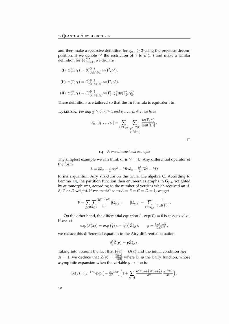
1.4 A one-dimensional example

The simplest example we can think of is V = C. Any differential operator ofthe form

L = h∂x − 12 Ax2 − hBx∂x − h2

2 C∂2x − hD

forms a quantum Airy structure on the trivial Lie algebra C. According toLemma 1.5, the partition function then enumerates graphs in Gg,n, weightedby automorphisms, according to the number of vertices which received an A,B, C or D weight. If we specialize to A = B = C = D = 1, we get

F = ∑g≥0

∑n≥1

hg−1xn

n!|Gg,n|, |Gg,n| = ∑

Γ∈Gg,n

1|aut(Γ)| .

On the other hand, the differential equation L · exp(F) = 0 is easy to solve.If we set

exp(F(x)) = exp( 1

h (x− x2

2 ))Z(y), y = 1−2x−h

(2h)2/3 ,

we reduce this differential equation to the Airy differential equation

∂2yZ(y) = yZ(y) .

Taking into account the fact that F(x) = O(x) and the initial condition F0,3 =

A = 1, we deduce that Z(y) = Bi(y)Bi(0) where Bi is the Bairy function, whose

asymptotic expansion when the variable y→ +∞ is

Bi(y) = y−1/4 exp(− 2

3 y3/2)(1 + ∑m≥1

6mΓ(m+ 16 )Γ(m+ 5

6 )2π

y−3m/2

m!

).

12

1.5. Operations on quantum Airy structures

Note that logarithm of Z(y) has an asymptotic expansion when y→ ∞ whichbecomes an element of EV once we substitute y = (2h)−2/3(1− 2x − h) andconsider the result as a formal series in h and x. It is only in this sense thatthe Bairy function “computes” the generating series of trivalent graphs. Thisis actually a well-known result. For general A, B, C, D, one can still solve thedifferential equation L · exp(F) = 0, and the result is expressed in terms of theWhittaker-M function, see [2].

The appearance of the Airy differential equation here motivates the name“quantum Airy structure”.

1.5 Operations on quantum Airy structures

The group exp(WV(≤ 2)) acts on its Lie algebra WV(≤ 2) by conjugation.So, if L : V → WV(≤ 2) is a quantum Airy structure, we can consider forU ∈ exp(WV(≤ 2)) the new system of differential operators and the partitionfunction it annihilates

(10) L→ L = ULU−1, Z → Z = UZ .

Yet, for a general U, ULU−1 will not be a quantum Airy structure. Apart fromh-degrees, the main obstruction is that L should contain as linear terms onlyderivations and no linear terms xi. We shall describe three such operations thatdo preserve quantum Airy structures. When this is so, it is for a conjugated(thus isomorphic) Lie algebra structure on V. The resulting transformation(A, B, C, D)→ (A, B, C, D) can be explicitly thanks to

1.6 lemma. Let (ui,j)i,j∈I be a symmetric matrix, V = (vi,j)i,j∈I be a matrix, and(ti)i∈I a vector. We have

exp(− h2 ua,b∂xa ∂xb)taxa exp

( h2 ua,b∂xa ∂xb

)= taxa + hua,bta∂xb +

h2 ua,btatb ,

exp(− 12h ua,bxaxb

)hta∂xa exp

( 12h ua,bxaxb

)= hta∂xa − ua,btaxb +

12 ua,btatb ,

exp(−va,bxa∂xb)xi exp(va,bxa∂xb) = (e−V)a,ixa ,

exp(−va,bxa∂xb)hta∂xa exp(va,bxa∂xb) = (eV)i,a h∂xa .

Proof. Let X, Y be elements of a Lie algebra such that [X, [X, Y]] is central. TheBaker-Campbell-Hausdorff formula in this special case implies

exp(−X)Y exp(X) = Y− [X, Y] + 12 [X, [X, Y]] .

We apply it to the Lie algebra WV(≤ 2). With X = h2 ua,b∂xa ∂xb and Y = taxa,

we compute [X, Y] = hua,bta∂xb and [X, [X, Y]] = hua,btatb which is indeedcentral, and this leads to the first claim. With X = 1

2h ua,bxaxb and Y = hta∂xa ,we compute [X, Y] = −ua,btaxb and [X, [X, Y]] = −ua,btatb which is central,and this leads to the second claim.

Now, we consider X = va,bxa∂xb and introduce the vector Y = (Yi)i∈I withYi = xi. We compute [X, Yi] = vi,axa. Commuting further with X does not givea central element, so we have to use another method. Let us work over K[[z]]

13


instead of K. Setting G(z) = exp(−zX)Y exp(zX), we compute

∂zG(z) = − exp(−zX)[X, Y] exp(zX) = −VTG(z), G(0) = Y ,

which is solved by G(z) = exp(−zVT)Y. Specializing to z = 1 replaces K byK and gives the third claim – if dim V = ∞, one must assume convergence.The fourth claim is proved in a similar way.

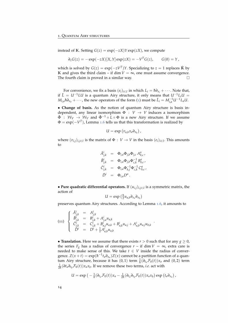
For convenience, we fix a basis (ei)i∈I in which Li = h∂xi + · · · . Note that,if L = U−1LU is a quantum Airy structure, it only means that U−1LiU =Mi,a h∂xa + · · · , the new operators of the form (1) must be Li = M−1

i,a U−1LaU.

• Change of basis. As the notion of quantum Airy structure is basis in-dependent, any linear isomorphism Φ : V → V induces a isomorphismΦ : WV → WV and Φ−1 L Φ is a new Airy structure. If we assumeΦ = exp(−VT), Lemma 1.6 tells us that this transformation is realized by

U = exp(va,bxa∂xb

),

where (vi,j)i,j∈I is the matrix of Φ : V → V in the basis (ei)i∈I . This amountsto

Aij,k = Φi,aΦj,bΦj,c Aa

b,c ,

Bij,k = Φi,aΦj,bΦ−1

c,k Bab,c ,

Cij,k = Φi,aΦ−1

b,j Φ−1c,k Ca

b,c ,

Di = Φi,aDa .

• Pure quadratic differential operators. If (ui,j)i,j∈I is a symmetric matrix, theaction of

U = exp( h

2 ua,b∂xa ∂xb

)

preserves quantum Airy structures. According to Lemma 1.6, it amounts to

(11)

Aij,k = Ai

j,kBi

j,k = Bij,k + Ai

j,aua,k

Cij,k = Ci

j,k + Bia,jua,k + Bi

a,kua,j + Aia,bua,jub,k

Di = Di + 12 Ai

a,bua,b

.

• Translation. Here we assume that there exists r > 0 such that for any g ≥ 0,the series Fg has a radius of convergence r – if dim V = ∞, extra care isneeded to make sense of this. We take t ∈ V inside the radius of conver-gence. Z(x + t) = exp(h−1ta∂xa)Z(x) cannot be a partition function of a quan-tum Airy structure, because it has (0, 1) term 1

h (∂taF0(t))xa and (0, 2) term1

2h (∂ta∂tbF0(t))xaxb. If we remove these two terms, i.e. act with

U = exp(− 1

h (∂taF0(t))xa − 12h (∂ta ∂tbF0(t))xaxb

)exp

(ta∂xa

),

14

1.6. Bonus: from classical to quantum Airy structures

then we obtain a new quantum Airy structure. By consistency it must have

Aij,k = ∂ti ∂tj ∂tkF0(t), Di = ∂tiF1(t) .

The transformation of B and C is computed by changing directly x → x + t

Bij,k = (M−1)i,a

(Ba

j,k + Cak,b∂tj ∂tbF0(t)

),

Cij,k = (M−1)i,aCa

j,k ,

Di = (M−1)i,aDa .

where Mi,j = δi,j − Bij,ata − Ci

j,a∂taF0(t).It can also be checked directly that if (A, B, C, D) is solution of the six

relations (3)-(4)-(5), then for each of the transformations above, (A, B, C, D) isa solution of the six relations as well.

• Direct sum. There is a last obvious operation we can do if we dispose ofa family of quantum Airy structure L(α) : V() → WV(α) indexed by α, withpartition function Z(α): the direct sum

⊕α L(α) is a quantum Airy structure on⊕

α V(α), with partition function ∏α Z(α).

1.6 Bonus: from classical to quantum Airy structures

The motivation of Kontsevich and Soibelman to introduce quantum Airystructures comes from an interpretation of tr as a quantization of quadraticLagrangians in the symplectic vector space T∗V.

• Classical Airy structures. For simplicity we assume V finite-dimensionaland K = R or C. Denote (xi)i∈I linear coordinates on V, and (yi)i∈I the cor-responding linear coordinates on V∗. We equip T∗V with its canonical sym-plectic structure ω, and denote ·, · the corresponding Poisson bracket

∀i, j ∈ I, xi, xj = yi, yj = 0, yi, xj = δi,j .

1.7 definition. A classical Airy structure is the data of scalars Aij,k = Ai

k,j, Bij,k,

Cij,k and f k

i,j = − f ki,j such that the family of functions (λi)i∈I on T∗V defined

(12) λi = yi − 12 Ai

a,bxaxb − Bia,bxayb − 1

2 Cia,byayb

satisfy λi, λj = f ai,jλa for all i, j ∈ I.

A classical Airy structure is thus characterized by (A, B, C, f ) satisfying thefive relations (3) and (5).

1.8 lemma. If (A, B, C, f ) is a classical Airy structure, then the subvariety Λ =(x, y) ∈ T∗V : ∀i ∈ I, λi(x, y) = 0 is a Lagrangian in a neighborhood of0 ∈ T∗V.

Proof. Let X(i) be the hamiltonian vector field of λi. The function λi, λj =

15


f ai,jλa vanishes on Λ. This is also equal to X(i), X(j) = dλi(X(j)), which thus

vanishes on Λ. Therefore, the restriction of X(j) to Λ is a tangent vector fieldto Λ. In a neighborhood of 0, (dλi)i∈I are linearly independent. Therefore, Λrestricted to this neighborhood is a manifold of dimension 1

2 dim V, whosetangent space is spanned by (X(i))i∈I . Hence it is Lagrangian.

•Quantization. The Weyl algebraWV provides a canonical deformation quan-tization of the Poisson manifold T∗V, i.e. an algebra over K[[h]] with a linearprojection map p : WV → K[T∗V] such that

[X, Y] = hp(X), p(Y)+ O(h2) .

Quantizing a Lagrangian Λ ⊂ T∗V then means constructing aWV-module Λ,which in the limit h→ 0 becomes the ring of functions on Λ, i.e. K[T∗V]/λi =0. Here, we are only considering Lagrangians of T∗V defined by quadraticequations of the form (12). Finding such Lagrangians is a non-trivial task, asone has to solve in particular the three quadratic relations (5). But if we imag-ine that we have found one Λ, completing (A, B, C) to a quantum Airy struc-ture (A, B, C, D) is fairly easy as it just requires solving the affine equation (4)for D (see the remark at the end of this lecture). In fact, if we want to quantizethe monomials xiyj in the λs, we have two choices h xi∂xj and h ∂xj xi, whichdiffer by a constant times h. The choice of D can be seen as a prescription forquantization of those monomials, but it is not arbitrary, as we desire that thequantization λi Li lifts the Poisson commutation relation to commutationrelations. The resulting constraint on D is (4). If we find such a quantum Airystructure L : V → WV , we then get a WV-module Λ = WV/L.WV whichquantizes the Lagrangian Λ in the above sense.

The space exp(EV) of formal functions on V defined in (6) is anotherWV-module. We can then consider the space HomWV

(WV/L.WV , exp(EV)

), which

is isomorphic as a vector space to the space of solutions of L(v).Z = 0 for allv ∈ V. The partition function of the quantum Airy structure is an elementof this vector space, which generates it under the action of exp(WV(≤ 2)).Sometimes, such a Z is also called “wave function”.

• A representation theory perspective on classical Airy structures. We revisitthe five relations in (3) and (5) which characterize classical Airy structures. IfL : V → WV(≤ 2) is an arbitrary linear map, we can study the commutatormap ρ : V → End(T∗V) obtained by considering T∗V ⊂ WV(1) and

∀w ∈ T∗V, ρ(v)(w) = h−1[L(v), w] .

We note that ρ is not sensitive to the presence of constants in L, it only dependson the coefficients (A, B, C). Let us compute its matrix in a basis in which Lihas the form (1), that is the basis xi for V∗ ⊂ WV(1), and h∂xi for V ⊂ WV(1).We find

(13) ρi =

( −Bi Ai

Ci (Bi)T

),

16

1.6. Bonus: from classical to quantum Airy structures

where we decomposed T∗V = V∗ ⊕ V, and Xi is the matrix (Xij,k)j,k∈I . We

therefore find that ρ(v) belongs to sp(T∗V), the Lie algebra of symplecticmatrices in T∗V – equipped with its canonical symplectic structure.

1.9 lemma. A classical Airy structure is equivalent to the data of a Lie algebra struc-ture on V and a Lagrangian embedding ϕ : V → T∗V, together with a Lie algebrarepresentation ρ : V → sp(T∗V) such that

(14) ∀v1, v2 ∈ V, ρ(v1)(ϕ(v2))− ρ(v2)(ϕ(v2)) = ϕ([v1, v2]) .

Proof. ρ is a representation if and only if we have ρ([v1, v2]) = [ρ(v1), ρ(v2)]for any v1, v2 ∈ V. Let us choose a basis (ei)i∈I of the abstract vector spaceV, which we transport with ϕ to a basis still denoted (ei)i∈I of V ⊂ T∗V,in which L(ei) takes the form (13). Making explicit the condition that ρ is arepresentation and that (14) holds, yields exactly the five conditions (3)-(5).

By analogy with the condition for Riemannian connections acting on vectorfields, we may call (14) a zero-torsion condition.

• Quantizing Airy structures. To lift a classical Airy structure (A, B, C) to aquantum Airy structure, we need a D ∈ HomK(V, K) solution of (4). As it isan affine relation, if D0 is a solution, then D is another solution if and only iff ai,j(Da − Da

0) = 0. In other words, D is another solution iff

(D− D0)([V, V]) = 0 .

To conclude, let us say that when V is finite-dimensional, one can check thatDi

0 = 12 ∑k∈I Bi

k,k is always a solution of (4). Indeed, in this case (4) is impliedby taking k = ` and summing over k ∈ I in the second relation of (5).

17

2. Two-dimensional topological quantum field theories


2 Two-dimensional topological quantum field theories

2.1 Definitions

• The category Bord2. Its objects are finite disjoint union of topological, com-pact, oriented, connected 1-manifolds. If B1, B2 are two objects, the morphismsB1 → B2 are equivalence classes of compact oriented surfaces Σ, with orientedboundaries1 such that the set of boundaries of Σ whose orientation disagreewith the orientation induced from Σ is ∂−Σ = B1, and the set of boundarieswhose orientation agree is ∂+Σ = B2. Here we say that Σ is equivalent toΣ′ if there exists a diffeomorphism ϕ : Σ → Σ′ preserving the orientationof Σ and of the boundaries. If B1, B2, B3 are three objects, [Σ1] is a morphismfrom B1 → B2 and [Σ2] is a morphism from B2 to B3, we choose a parametriza-tion (i.e. a diffeomorphism to the standard S1) of each connected component of∂+Σ1 and of ∂−Σ2, and form a surface Σ1,2 by glueing together ∂+Σ1 and ∂−Σ2such that the parametrizations match. The choice of parametrization was nec-essary to perform a glueing, but the resulting equivalence class [Σ1,2] does notdepend on this choice, neither on the choice of representatives Σ1 and Σ2. Thisallows the definition of the composition of morphisms [Σ2] [Σ1] = [Σ1,2]. Thedisjoint union induces a monoidal structure on Bord2, for which the emptydisjoint union is the unit object.

The morphisms in this category are generated under composition by basicsurfaces of genus 0, with n ≤ 3 boundaries – which can be either negativelyor positively oriented. Note that the cylinder with one negatively orientedboundary, and one positively oriented boundary, represents the identity mor-phism of the object S1 appearing at the boundaries.

• The category VectK. Its objects are finite-dimensional K-vector spaces, andits morphisms are K-linear maps. The tensor product induces a monoidalstructure on VectK, for which K is the unit object.

• 2d TQFTs. A two-dimensional topological quantum field theory is a monoidalfunctor F : Bord2 → VectK. This axiomatization is due to Atiyah [4], and canbe done in any dimension d, using a category Bordd whose objects are (d− 1)-manifolds and morphisms are equivalence classes of d-manifolds.

• Frobenius algebras. A Frobenius algebra A is a finite-dimensional K-vectorspace equipped with the structure of a commutative associative algebra µ :A⊗A → A with a unit 1 : K→ A, and a non-degenerate symmetric pairingb : A⊗A → K such that the product is invariant

∀a1, a2, a3 ∈ A, b(µ(a1 ⊗ a2), a3) = b(a1, µ(a2 ⊗ a3)) .

1What we call boundary throughout the text is, more precisely speaking, a boundary compo-nent.

18

2.2. Correspondence with Frobenius algebras

2.2 Correspondence with Frobenius algebras

An important idea in the mathematical approach to quantum field theories isthat manifolds and their glueings give rise to algebraic structures, where al-gebraic relations express diffeomorphisms between manifolds. The followingresult has been folklore knowledge, and it seems to have been written in detailfor the first time in [1]. The negatively oriented boundaries are drawn to theleft, and the positively oriented ones to the right.

2.1 theorem. A 2d tqft determines a Frobenius algebra structure on F (S1) = Avia the formulas

F( )

= µ : A⊗A → A

F( )

= b : A⊗A → K

F( )

= 1 : K→ A

Conversely, for any Frobenius algebras, these formulas determine a unique 2d tqft.

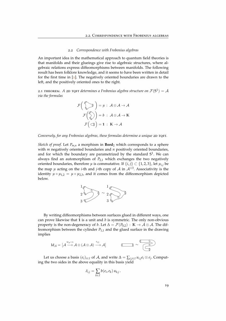
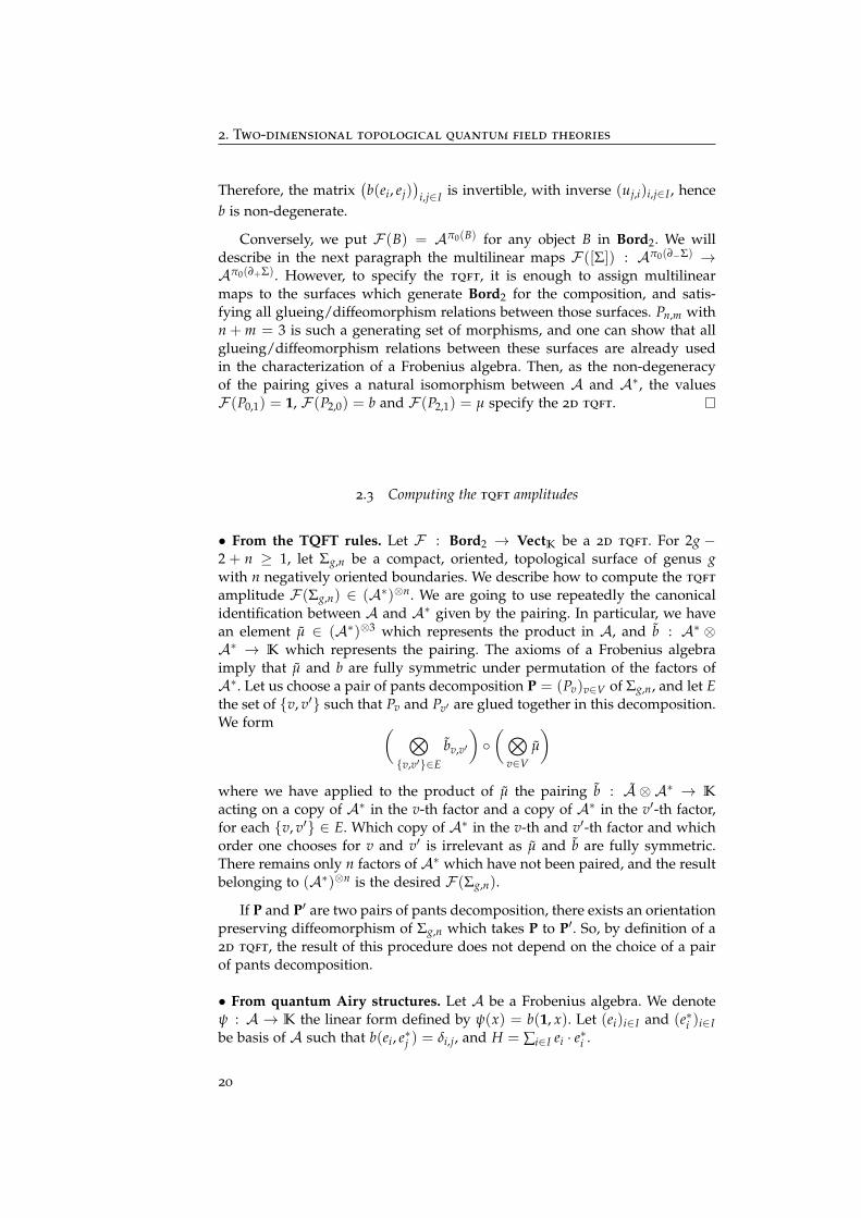
Sketch of proof. Let Pm,n a morphism in Bord2 which corresponds to a spherewith m negatively oriented boundaries and n positively oriented boundaries,and for which the boundary are parametrized by the standard S1. We canalways find an automorphism of P2,1 which exchanges the two negativelyoriented boundaries, therefore µ is commutative. If i, j ⊂ 1, 2, 3, let µi,j bethe map µ acting on the i-th and j-th copy of A in A⊗3. Associativity is theidentity µ µ1,2 = µ µ2,3, and it comes from the diffeomorphism depictedbelow.

1

2

3

2

1

3

∼

By writing diffeomorphisms between surfaces glued in different ways, onecan prove likewise that 1 is a unit and b is symmetric. The only non-obviousproperty is the non-degeneracy of b. Let ∆ = F (P0,2) : K→ A⊗A. The dif-feomorphism between the cylinder P1,1 and the glued surface in the drawingimplies

∼IdA =[A −→ A⊗ (A⊗A) −→ A

]IdA ⊗ ∆ b1,2

Let us choose a basis (ei)i∈I of A, and write ∆ = ∑i,j∈I ui,jei ⊗ ej. Comput-ing the two sides in the above equality in this basis yield

δi,j = ∑k∈I

b(ei, ek) uk,j .

19

2. Two-dimensional topological quantum field theories

Therefore, the matrix(b(ei, ej)

)i,j∈I is invertible, with inverse (uj,i)i,j∈I , hence

b is non-degenerate.

Conversely, we put F (B) = Aπ0(B) for any object B in Bord2. We willdescribe in the next paragraph the multilinear maps F ([Σ]) : Aπ0(∂−Σ) →Aπ0(∂+Σ). However, to specify the tqft, it is enough to assign multilinearmaps to the surfaces which generate Bord2 for the composition, and satis-fying all glueing/diffeomorphism relations between those surfaces. Pn,m withn + m = 3 is such a generating set of morphisms, and one can show that allglueing/diffeomorphism relations between these surfaces are already usedin the characterization of a Frobenius algebra. Then, as the non-degeneracyof the pairing gives a natural isomorphism between A and A∗, the valuesF (P0,1) = 1, F (P2,0) = b and F (P2,1) = µ specify the 2d tqft.

2.3 Computing the tqft amplitudes

• From the TQFT rules. Let F : Bord2 → VectK be a 2d tqft. For 2g −2 + n ≥ 1, let Σg,n be a compact, oriented, topological surface of genus gwith n negatively oriented boundaries. We describe how to compute the tqft

amplitude F (Σg,n) ∈ (A∗)⊗n. We are going to use repeatedly the canonicalidentification between A and A∗ given by the pairing. In particular, we havean element µ ∈ (A∗)⊗3 which represents the product in A, and b : A∗ ⊗A∗ → K which represents the pairing. The axioms of a Frobenius algebraimply that µ and b are fully symmetric under permutation of the factors ofA∗. Let us choose a pair of pants decomposition P = (Pv)v∈V of Σg,n, and let Ethe set of v, v′ such that Pv and Pv′ are glued together in this decomposition.We form ( ⊗

v,v′∈E

bv,v′

)(⊗

v∈Vµ

)

where we have applied to the product of µ the pairing b : A ⊗ A∗ → K

acting on a copy of A∗ in the v-th factor and a copy of A∗ in the v′-th factor,for each v, v′ ∈ E. Which copy of A∗ in the v-th and v′-th factor and whichorder one chooses for v and v′ is irrelevant as µ and b are fully symmetric.There remains only n factors of A∗ which have not been paired, and the resultbelonging to (A∗)⊗n is the desired F (Σg,n).

If P and P′ are two pairs of pants decomposition, there exists an orientationpreserving diffeomorphism of Σg,n which takes P to P′. So, by definition of a2d tqft, the result of this procedure does not depend on the choice of a pairof pants decomposition.

• From quantum Airy structures. Let A be a Frobenius algebra. We denoteψ : A → K the linear form defined by ψ(x) = b(1, x). Let (ei)i∈I and (e∗i )i∈Ibe basis of A such that b(ei, e∗j ) = δi,j, and H = ∑i∈I ei · e∗i .

20

2.3. Computing the tqft amplitudes

2.2 lemma. The following data

Aij,k = ψ(e∗i · e∗j · e∗k ) ,

Bij,k = ψ(e∗i · e∗j · ek) ,

Cij,k = ψ(e∗i · ej · ek) ,

Di = ψ(e∗i · H) ,

defines a quantum Airy structure on the abelian Lie algebra A. Besides, for 2g −2 + n > 0 the amplitudes of the 2d tqft associated to A are computed by the tr

amplitudes of this quantum Airy structure through

(15) F (Σg,n) = |Gg,n|Fg,n .

In other words, the tensors (A, B, C) in this quantum Airy structure allrepresent the product in A.

Proof. For simplicity, let us assume that ei is an orthonormal basis. Orthogonalbasis always exist, but to obtain an orthonormal basis we may have to replaceK by an extension K. The final result however, is insensitive to this detail. Inthis case, we have e∗i = ei and

Aij,k = Bi

j,k = Cij,k ,

which is fully symmetric. The three relations (5) are then identical, and wejust need to check one of them. In the IHX representation, each vertex is an Aand the ordering of the edges at the vertices is irrelevant. When we permutethe indices i and j, the H-graph is sent to itself, while the I- and X-graphare swapped. Therefore, (5) is satisfied in a rather simple way. Then, by fullsymmetry of B, we have f k

i,j = 0: the underlying Lie algebra is abelian. As aconsequence, the first term in (4) involving D is automatically symmetric, andas Ai

j,k = Cij,k (4) is satisfied for any D ∈ HomK(A, K).

For 2g− 2 + n = 1, there is a single graph in Gg,n, and it has trivial auto-morphism group. By construction, F0,3 = A = F (Σ0,3) represents the product,and we choose Di = F (Σ1,1)(ei) so that (15) holds for (g, n) = (1, 1). It is moreexplicitly computed by decomposing the torus with one boundary as a self-glued pair of pants.

The rules given above then give F (Σ1,1)(ei) = ψ(ei H) with H = ∑j∈I ej · ej.Now consider 2g − 2 + n ≥ 2. To any Γ ∈ Gg,n, we can associate a pair

of pants decomposition PΓ of Σg,n as in the picture below. A coloring of Γ isthe assignment of an element of the basis to each edge/leaf, and since A, Band C are equal when written in the orthonormal basis, the contribution ofeach trivalent vertex v to the weight is always the product of all the vectors

21

3. Intersection theory on the moduli space of curves

carried by edges incident to that vertex – when represented as an elementof A⊗3 → K. Moreover, summing over the colors of the edges amounts toperform a pairing because

∀x, y ∈ A, ∑a

ψ(xea)ψ(eay) = ψ(xy) ,

when we use the orthonormal basis (ei)i∈I . And, when Γ has a loop, there is aself-glued pair of pants, which we can consider as a torus with one boundary,having by definition a contribution Di if the loop is color by i.

Comparing with the tqft rules, we find that the sum over all colorings ofΓ which assigns the colors (i1, . . . , in) to the n-leaves coincide with the tqft

amplitude computed from the pair of pants decomposition PΓ, evaluated atei1 ⊗ · · · ⊗ ein . Since this amplitude does not depend on the pair of pants de-composition, the number of graphs (weighted by automorphisms) factorizesin the computation of the tr amplitude

Fg,n = ∑Γ∈Gg,n

∑γ∈IE′(Γ)γ(`j)=ij

w(Γ, γ)

|aut(Γ)|

= ∑Γ∈Gg,n

F (Σg,n)(ei1 ⊗ · · · ⊗ ein)

|aut(Γ)| = |Gg,n| F (Σg,n)(ei1 ⊗ · · · ⊗ ein) .

3 Intersection theory on the moduli space of curves

3.1 A quantum Airy structure on the loop space

• Definition. We describe a quantum Airy structure on V = zC[[z2]]. We takeas basis of V

ξ∗k =z2k+1

(2k + 1)!!,

indexed by k ∈N. We also introduce

(16) ξk =(2k + 1)!!

z2k+2 dz ,

and take θ ∈ z−2C[[z2]].(dz)−1 which we decompose as

θ = ∑r≥−1

θr z2r (dz)−1 ,

22

3.1. A quantum Airy structure on the loop space

with the convention θr = 0 for r ≤ −2.

3.1 theorem. The following data

(17)

Aij,k = Res 0

(ξ∗i · dξ∗j · dξ∗k · θ

)= δi,j,k,0θ−1 ,

Bij,k = Res 0

(ξ∗i · dξ∗j · ξk · θ

)= (2k+1)!!

(2i+1)!!(2j+1)!! (2j + 1) θk−i−j ,

Cij,k = Res 0

(ξ∗i · ξ j · ξk · θ

)= (2k+1)!!(2j+1)!!

(2i+1)!! θk+j+1−i ,

Di = θ−124 δi,0 +

θ08 δi,1 ,

defines a quantum Airy structure on V ∼= ⊕k≥0 C.ξ∗k . If we denote r0 = minr ≥

−1 : θr 6= 0, the Lie algebra structure it induces on V is isomorphic to a sub-Liealgebra spanned by (Lk)k≥r0 of the Lie algebra Witt+, which is spanned by (Lk)k∈≥1with commutation relations

(18) ∀k, ` ∈ Z, [Lk,L`] = (k− `)Lk+` .

In particular, in the generic case θ−1 6= 0, we get a Lie algebra isomorphicto L−1,L0,L1, . . ., which is the Lie algebra of change of coordinates in theformal disk at 0 in C.

Proof. I do not know an elegant proof of this result: one can check by directcomputation that the six relations (3)-(5)-(4) are satisfied. Note that Bi

j,k = 0

whenever i + j > k + 1, and Cij,k = 0 whenever i > j + k + 2, and this implies

that all sums over indices a ≥ 0 appearing in (5) contain only finitely non-zeroterms. Let us focus on identifying the Lie algebra. We have

(19) [Li, Lj] = ∑k≥0

(2k + 1)!!(2i + 1)!!(2j + 1)!!

2(j− i)θk−i−j Lk .

If we decomposezr0

θ= ∑

k≥0τk zk dz ,

and defineLi = − ∑

k≥0τk Li+k−r0 , , Li =

(2i+1)!!2 Li ,

computation shows that the commutations (19) imply

[Li,Lj] = (i− j)Li+j .

• Symplectic point of view. There is an analogy with the structure of (A, B, C)in this quantum Airy structure and that described for tqfts: A, B, C are alwaysthe result of applying the trace form to a triple product. The trace form ψof a Frobenius algebra is replaced here by the formal residue at 0, and theproduct is the usual product of formal Laurent series. The vector space W =

23


C[z−2, z2]].dz ' T∗V admits a symplectic structure

ω( f , g) = Res0

(fˆ

g)

,

and d : V → W is a linear Lagrangian embedding. (ξk)k≥0 defined in (16)are elements of W, and they also span a Lagrangian subspace V′ of W, sothat we get a Lagrangian splitting W ' dV ⊕ V′, and (ξk)k≥0 was preciselychosen such that it forms together with (ξ∗k ) a symplectic basis adapted to thissplitting

ω(ξk, dξ∗` ) = δk,` .

If (ui,j)i,j≥0 is a symmetric semi-infinite matrix, we can transform thisquantum Airy structure by conjugation by exp


)as described in

Section 1.5. Comparing (11) with (17), we see that this transformation amountsto

ξk → ξk + uk,adξ∗a .

In other words, it changes the supplement subspace V′ in the Lagrangiansplitting W ' dV ⊕V′.

3.2 Witten-Kontsevich partition function

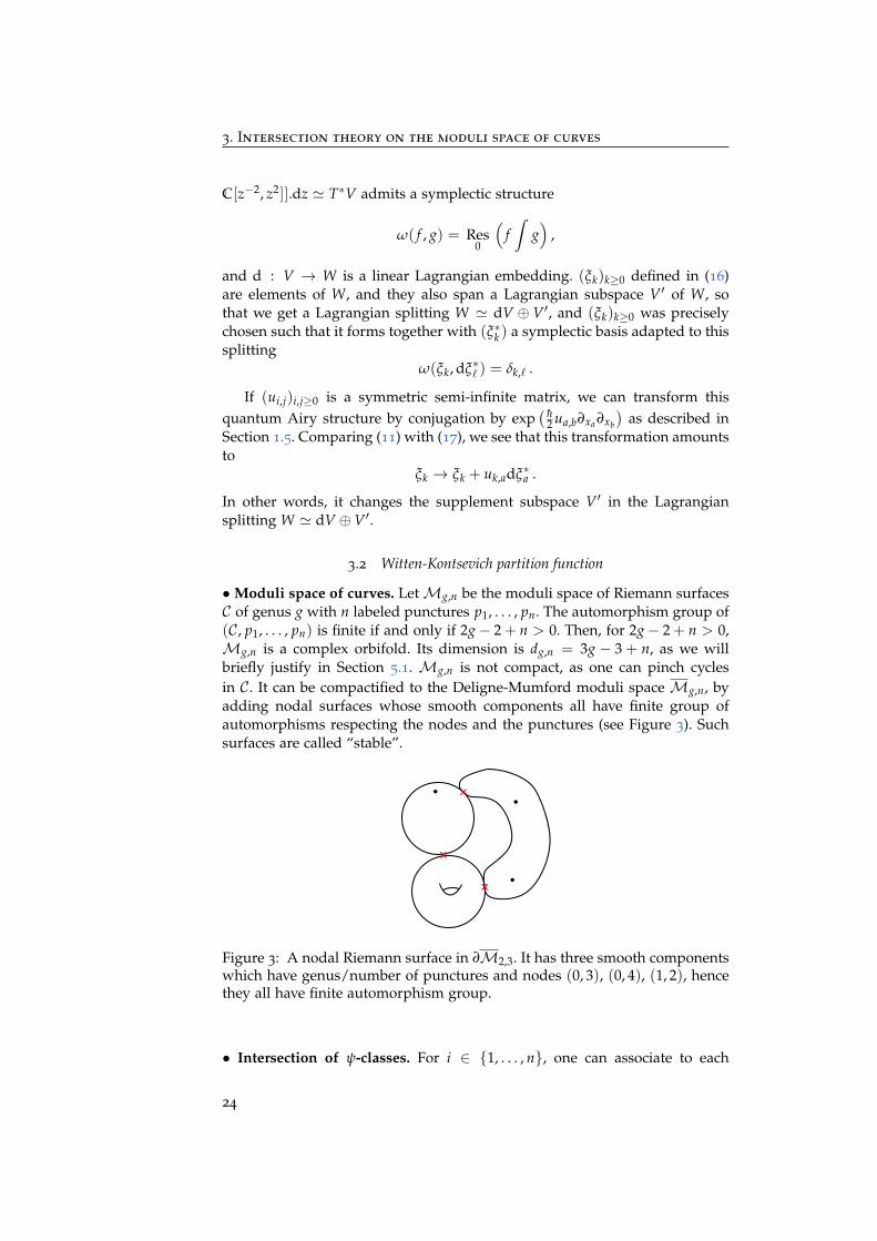
•Moduli space of curves. LetMg,n be the moduli space of Riemann surfacesC of genus g with n labeled punctures p1, . . . , pn. The automorphism group of(C, p1, . . . , pn) is finite if and only if 2g− 2 + n > 0. Then, for 2g− 2 + n > 0,Mg,n is a complex orbifold. Its dimension is dg,n = 3g − 3 + n, as we willbriefly justify in Section 5.1. Mg,n is not compact, as one can pinch cyclesin C. It can be compactified to the Deligne-Mumford moduli space Mg,n, byadding nodal surfaces whose smooth components all have finite group ofautomorphisms respecting the nodes and the punctures (see Figure 3). Suchsurfaces are called “stable”.

Figure 3: A nodal Riemann surface in ∂M2,3. It has three smooth componentswhich have genus/number of punctures and nodes (0, 3), (0, 4), (1, 2), hencethey all have finite automorphism group.

• Intersection of ψ-classes. For i ∈ 1, . . . , n, one can associate to each

24

3.2. Witten-Kontsevich partition function

(C, p1, . . . , pn) ∈ Mg,n the complex one-dimensional space T∗piC. It forms

over Mg,n a holomorphic line bundle, and its first Chern class is a coho-mology class in H2(Mg,n, Q) denoted ψi. We also have fundamental class[1] ∈ H0(Mg,n, Q), which is characterized by

ˆMg,n

[1] = 1 .

We take the convention ψ0i = [1], and if ω is a cohomology class which does

not have top degree 3g− 3 + n, we set´Mg,n

ω = 0.

3.2 theorem. Choose θ = z−2(dz)−1 in the quantum Airy structure (17). The tr

amplitudes then compute the ψ-classes intersections

∀k1, . . . , kn ≥ 0, Fg,n[k1, . . . , kn] =

ˆMg,n

ψk11 ∪ · · · ∪ ψkn

n .

We denote ZWK the corresponding partition function.

This theorem means that the generating series

Z = exp

∑g≥0

∑n≥1

∑k1,...,kn≥0

hg−1

n!

( ˆMg,n

ψk11 ∪ · · · ∪ ψkn

n

)xk1 · · · xkn

,

satisfies the differential equations Li · Z = 0 for all i ≥ −1, where the lowestLi = Li−1 are equal to

L−1 = h∂x0 − 12 x2

0 − ∑k≥0

hxk∂xk+1 ,

L0 = h∂x1 − ∑k≥0

h 2k+13 xk∂xk − h

24 ,

L1 = h∂x2 − ∑k≥0

h (2k+3)(2k+1)15 xk∂xk+1 − h2

30 ∂2x0

.

The constraints L−1 · Z = 0 are L0 · Z = 0 can be proved in an elementaryway and are called the string and dilaton equation. As M0,3 is a point withno automorphism, we have

F0,3[i, j, k] =ˆM0,3

[1] = 1 .

With this as initial data, the string equation recursively determines all ψ-classes intersections. The result reads

ˆM0,n

ψk11 ∪ · · · ∪ ψkn

n =

(n−3)!k1!···kn ! if ∑i ki = n− 30 otherwise

.

25


It is also an elementary result in algebraic geometry thatˆM1,1

ψ1 = 124 ,

and this is indeed the value assigned to D0 in Theorem 3.2. The equationL1 · Z = 0 is already non-trivial. This result is implied by the conjecture ofWitten [27] that Z is a KdV tau function satisfying the string equation, provedby Kontsevich in [18].

26

4 Cohomological field theories

4.1 Definition

• Axioms. Let A be a Frobenius algebra over C. A cohomological field the-ory (cohft) on A is a sequence of linear maps Ωg,n : A⊗n → H•(Mg,n, C)indexed by integers g ≥ 0 and n ≥ 1 such that 2g− 2 + n > 0, satisfying thefollowing axioms.

• Ωg,n is symmetric under permutation of the n factors of A.

• Ω0,3 : A⊗3 → H•(M0,3, C) ∼= C represents the product in A.

• Ωs are compatible with all natural morphisms between moduli spacesof curves, in a sense spelled out below.

• Morphisms between Mg,ns. The list of these natural morphisms is as fol-lows. First, we can forget the last puncture, obtaining maps

π0 : Mg,n+1 −→Mg,n .

We then require

π∗0 Ωg,n(v1 ⊗ · · · ⊗ vn) = Ωg,n+1(v1 ⊗ · · · ⊗ vn ⊗ 1) .

Second, if (p, q) is an ordered pair of points on a stable Riemann surface,we can glue them so as to form a nodal surface. We obtain in this way twofamily of morphisms

πI : Mg−1,n+2 −→Mg,n ,

πII : Mg1,n1+1 ×Mg2,n2+1 −→Mg1+g2,n1+n2 .

p1

p2

p4

p3 p5

7−→tp1

p2

p4

p57−→

p1

p2

p3

p4p1

p2

p3

πII

πI

The image of these morphisms lies in the boundary of the target modulispace. In fact, the collection of all morphisms πI and πII is the collection ofinclusions of codimension 1 strata in the boundary of Mg,n. In other words,the interior of the source moduli space in these morphisms consists of theRiemann surfaces one can obtain by degenerating in the most generic way

27

4. Cohomological field theories

a Riemann surface in Mg,n. Let b† = ∑i∈I ei ⊗ e∗i be the element of A ⊗ Arepresenting the pairing in A. We then require that

(20) π∗I Ωg,n(v1 ⊗ · · · ⊗ vn) = ∑i∈I

Ωg−1,n+2(v1 ⊗ · · · · · · vn ⊗ ei ⊗ e∗i ) ,

and

π∗IIΩg1+g2,n1+n2(v1 ⊗ · · · ⊗ vn1+n2)

= ∑i

Ωg1,n1(v1 ⊗ · · · ⊗ vn1 ⊗ ei) ∪Ωg2,n2(vn1+1 ⊗ · · · ⊗ vn1+n2 ⊗ e∗i ) .

• CohFT partition function. To simplify the exposition, let us take (ei)i∈I0an orthonormal basis of A. If (Ωg,n)g,n is a cohft, we can form the partitionfunction Z = exp(F) with

(21)

F = ∑g≥0n≥1

hg−1

n! ∑i1,...,in∈I0k1,...,kn≥0

( ˆMg,n

Ωg,n(ei1 ⊗ · · · ⊗ ein)∪ψk11 ∪ · · · ∪ψkn

n

) n

∏j=1

xij ,kj,

which is a formal function on V = A[[z]]. Here xi,k indexed by (i, k) ∈ I =I0 ×N are the canonical linear coordinates on V, i.e. corresponding to thebasis eizk. The components Fg,n of (21) are called the cohft amplitudes.

• Degree 0 part. The restriction of a cohft to cohomological degree 0 yieldsmultilinear maps Ωdeg 0

g,n : A⊗n → H0(Mg,n, C) ∼= C. The axioms of the co-hft imply that these maps are completely determined by A. Indeed, we cancompute Ωdeg 0

g,n by degenerating any stable Riemann surface to a glueing ofspheres with 3 punctures only, and use the axioms. More precisely, comparingwith Section 2.3 we find that Ωdeg 0

g,n are the amplitudes of the tqft associatedto A. We also note that, if Ω is a cohft, so is Ωdeg 0.

• Remarks. If a cohft is not purely of cohomological degree 0, the axiomsgive constraints on the classes Ωg,n but do not determine them. In fact, thestructure of the ring H•(Mg,n) is rather complicated and still the theater ofactive research. So, there is little hope to classify cohfts in general. Yet, thestudy of cohfts gave recently (Pixton, Pandharipande, Zvonkine, and collabo-rators) new results about H•(Mg,n), and the classification in the case where Ais semi-simple has been completed through the work of Givental and Teleman.This is a deep result, which uses other difficult results on the cohomology ringH•(Mg,n, Q). We will explain below how this classification works.

• Prepotential and deformation of Frobenius algebras. We define the prepo-tential of a cohft as the formal function on A defined by restriction of thegenus 0 amplitude of the cohft

f0 = F0|xi,k=0 k≥1 .

28

4.2. Two examples.

We say that xi,0 are the “primary times”. Let us assume that f0 has a non-zeroradius of convergence, and take t ∈ A within the radius of convergence. Forsimplicity we also assume that 1 = e0 is an element of the orthonormal basis(ei)i∈I . One can prove from the cohft axioms that

µi1i2,i3

(t) =∂3f0

∂ti1,0∂ti2,0∂ti3,0(t) ,

bi1,i2(t) = µ0i2,i3 ,

determine tensors µ(t) : A ⊗ A → A and b(t) : A ⊗ A → C giving A at-dependent structure of Frobenius algebra. We thus obtain a family of Frobe-nius algebras, parametrized by a neighborhood N of 0 in A, which “derivefrom” the prepotential function f0. This has been axiomatized under the nameof Frobenius manifolds [9]. This notion plays an important role in enumerativegeometry, especially from the perspective of mirror symmetry and integrablehierarchies.

4.2 Two examples.

• Trivial CohFT. From the axioms, the fundamental class [1] ∈ H0(Mg,n, Q)is automatically a cohft on the trivial Frobenius algebra V = C. Its partitionfunction is by construction ZWK. Therefore, it is the partition function of thequantum Airy structure given in Theorem 3.1. If we choose ∆ ∈ C∗,

∆2g−2+n · [1] ∈ H0(Mg,n, Q)

is also a cohft, on the modified Frobenius algebra A∆ = C defined such thatthe element 1 ∈ C is orthonormal but 1 · 1 = ∆1. The partition function of thiscohft is

∆ZWK = ZWK(∆x)|h→h∆2 .

In fact, any one-dimensional Frobenius algebra must be isomorphic to A∆ forsome ∆ ∈ C∗.

• Chern character of bundles of conformal blocks. Two-dimensional rationalconformal field theory are axiomatized by the notion of modular functor – seee.g. [5]. We will not enter into the detail of these axiomatics, but rather state ofsome of its consequences. Let us fix a cft in this sense. There is a Frobeniusalgebra A spanned by a distinguished basis (εi)i∈I0 , which describes the possi-ble boundary conditions of the theory. For any g, n ≥ 0 and i1, . . . , in ∈ I0, onecan then construct the bundle of conformal blocks Vg,n(i1, . . . , in) over Mg,n,and the cft axioms imply that this bundle enjoys factorization properties atthe boundary of the moduli space. This is the analog of the cohft axioms, butat the level of bundles. Then, their Chern character for 2g− 2 + n > 0 yield asequence of cohomology classes

Ωg,n(εi1 ⊗ · · · ⊗ εin) = Ch(Vg,n(i1, . . . , in))

which form a cohft [3]. Examples of cfts which fit in this formalism are

29


those constructed from modular tensor categories, from representations of thequantum group Uq(sl2) at q = exp( 2iπ

k+2 ) when k is a positive integer called“level”, etc. In the latter case, the construction of the bundle of conformalblocks comes from the pioneering work of [26]. For a general 2d rational cft,the existence of Vg,n(i1, . . . , in) seems to belong to folklore knowledge, and wewrote it in detail in [3].

4.3 Motivating example: quantum cohomology and Gromov-Witten theory

•Moduli space of stable maps. The notion of cohft was introduced by Kont-sevich and Manin [19] in an attempt to capture the properties of Gromov-Witten invariants. Let X be a smooth projective variety, fix g ≥ 0, n ≥ 1 andβ ∈ H2(X, Z). Consider the moduli space Mg,n(X, β) of maps φ : C →X from a stable Riemann surface C of genus g with n labeled punctures(p1, . . . , pn), such that [φ(C)] = β. This space is in general singular, but Behrendand Fantechi [6] and many others could construct a “virtual” fundamental cy-cle [Mg,n(X, β)]vir over which cohomology classes can be integrated, as if theywere integrated on a cycle of complex dimension

(22) dg,n(X, β) = dimC X + (3− dimC X)g + n− 3 +ˆ

βc1(TX) .

It is the analog of the homology cycle [Mg,n] which is Poincare dual to [1] inthe moduli space of curves.

• Gromov-Witten classes. This allows the definition of Gromov-Witten invari-ants, as follows. We have a proper fibration π : Mg,n(X, β) → Mg,n whichforgets about the map φ, and n morphisms evi : Mg,n(X, β) → X which re-member the image of pi via φ. For any v1, . . . , vn ∈ H•(X, C), we can form thecohomology class onMg,n

ΩX,βg,n (v1 ⊗ · · · ⊗ vn) = π∗

([Mg,n(X, β)]vir ∩

(ev∗1v1 ∪ · · · ∪ ev∗n(vn)

)),

which is called the Gromov-Witten theory class. Then, working in the Novikovring KX spanned by tβ for β = 2-cycles which can be realized as image of acurve, we can define

(23) ΩXg,n = ∑

β∈H2(X,Z)

tβ ΩX,βg,n .

• CohFTs and quantum cohomology. AX = H•(X, C) has the structure of aFrobenius algebra with the cup product and Poincare pairing. The propertiesof the Gromov-Witten invariants2 guarantee that ΩX

g,n is a cohft over AX incase the sum (23) is convergent – and over AX ⊗KX in general. Using theprepotential for this cohft, one can obtain a family of deformation of theFrobenius algebra structure on AX . The resulting ring is called “quantum

2Some being conjectural at the time of writing of [19] as the fundamental class had not beendefined yet.

30

4.4. Givental group action

cohomology ring” of X.

• Remarks. Note that when dimC X 6= 3, Gromov-Witten classes of high gen-era will vanish. So, for general varieties, the most interesting part of Gromov-Witten theory is the genus 0 part, and its restriction to primary times pro-vides the quantum cohomology of X. When X is a Calabi-Yau variety – i.e.c1(TX) = 0 – of complex dimension 3, the dimension (22) does not dependon β and g, so we have a priori infinitely many non-vanishing Gromov-Witteninvariants, and an important question is whether one can find an algorithmwhich can compute Gromov-Witten invariants in all genera and all degree.This question is at the heart of many developments in enumerative and al-gebraic geometry in the last 25 years, relating Gromov-Witten theory to inte-grable systems, modular forms, etc.

• Virasoro conjecture. Under an additional homogeneity assumption, Eguchi,Hori and Xiong with addition of Katz [11] proposed an explicit family (Lk)k≥−1of differential operators inWAX [[z]](≤ 2), which span a Lie algebra isomorphicto Witt+, and conjecturally annihilate the cohft partition function. Althoughsome cases have been proven, the general conjecture is still open, see [15] fora review. Although they take the form (1), these operators do not quite form aquantum Airy structure on AX [[z]], as we would rather need more operators(indexed by an integer k and basis elements i of AX) in order to get a quantumAiry structure.

4.4 Givental group action

Let us fix a Frobenius algebra A, and set V = A[[z]]. UsingWV(≤ 2) seen as aquantization of T∗V, Givental [16] and Coates constructed two operations oncohfts, called and R, which lift at the level of cohomology classes the actionof certain elements of the group exp(WV(≤ 2)) on the partition function. Thecomplete proof that R and T preserve the cohft axioms was only obtainedlater in [14].

• T operation. Let T ∈ z2A[[z]] ⊂ V, which we decompose as T(z) =

∑k≥2 Tkzk. If Ω is a cohft on A, we put

(TΩg,n)(v1 ⊗ · · · ⊗ vn)

= ∑m≥0

k1,...,km≥0

1m!

(πm)∗

(Ωg,n+m

( n⊗

i=1

vi ⊗m⊗

j=1

Tkj

)∪ ψk1

1 ∪ · · · ∪ ψknn

),

where we have introduced the morphism πm : Mg,n+m → Mg,n forgettingthe first m punctures. The pushforward (πm)∗(ω) here means that we takethe homology class dual to ω, push it forward, and then apply again Poincareduality to get a cohomology class. The effect on the cohft partition functionis a translation, as described in Section 1.5.

TZ(x) = exp(− 1

h∂taF0(T)xa

h − ∂ta tbF0(T)xaxb2h

)Z(x + T) .

31


• R-operation. Let R ∈ End(A[[z]]) ∼= End(A)[[z]] such that

(24) R = IdA + O(z) and R(z)R†(−z) = IdA ,

where † is the notion of adjoint induced by the pairing on A. We introducethe element B ∈ A⊗A[[z1, z2]] through

B(z1, z2) =b† − R(z1)⊗ R(z2)b†

z1 + z2.

The conditions (24) ensure that it is a well-defined formal power series in z1and z2. In general, if ω is a positive degree element of a cohomology ring H,we can evaluate an A-valued formal power series to an element of A⊗H byreplacing zk with the k-th power (for the cup product) of ω. The series willterminate as ω is nilpotent in H.

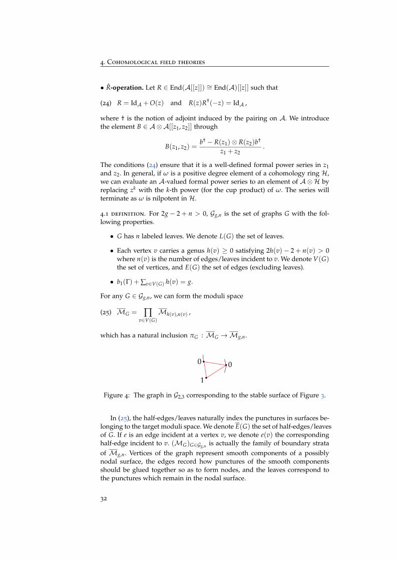
4.1 definition. For 2g− 2 + n > 0, Gg,n is the set of graphs G with the fol-lowing properties.

• G has n labeled leaves. We denote L(G) the set of leaves.

• Each vertex v carries a genus h(v) ≥ 0 satisfying 2h(v)− 2 + n(v) > 0where n(v) is the number of edges/leaves incident to v. We denote V(G)the set of vertices, and E(G) the set of edges (excluding leaves).

• b1(Γ) + ∑v∈V(G) h(v) = g.

For any G ∈ Gg,n, we can form the moduli space

(25) MG = ∏v∈V(G)

Mh(v),n(v) ,

which has a natural inclusion πG : MG →Mg,n.

0

1

0

Figure 4: The graph in G2,3 corresponding to the stable surface of Figure 3.

In (25), the half-edges/leaves naturally index the punctures in surfaces be-longing to the target moduli space. We denote E(G) the set of half-edges/leavesof G. If e is an edge incident at a vertex v, we denote e(v) the correspondinghalf-edge incident to v. (MG)G∈Gg,n is actually the family of boundary strataof Mg,n. Vertices of the graph represent smooth components of a possiblynodal surface, the edges record how punctures of the smooth componentsshould be glued together so as to form nodes, and the leaves correspond tothe punctures which remain in the nodal surface.

32

4.5. Semi-simple cohomological field theories

If Ω is a cohft on A, the R-operation is defined by

(RΩ)g,n = ∑G∈Gg,n

(πG)∗ Φ( ⋃

v,v′∈E(G)

B(ψe(v), ψe(v′)) ∪⋃

`∈L(G)

R(ψv)

).

Here, the result of the product between the round brackets is an element of

(A∗)⊗E(G) ⊗⊗

v∈V(G)

H•(Mh(v),n(v), C) ,

where we used the pairing to replace copies of A by A∗. The multilinear mapΦ applies the pairing on the glued half-edges so as to obtain an element of

(A∗)⊗L(G) ⊗⊗

v∈V(G)

H•(Mh(v),n(v), C) .

Finally, pushing forward via the morphism πG produces an element of

(A∗)⊗L(G) ⊗⊗

v∈V(G)

H•(Mg,n, C) .

This set of graphs is in fact tailored such that the action of this transforma-tion on the partition function is a composition of conjugation by exponential ofa pure quadratic differential operator (responsible for the weight of the edges)followed by a change of basis (responsible for the weights of the leaves). Letus choose an orthonormal basis (ei)i∈I0 of A, and denote (ua,b)a,b∈I0×N thecoefficients of B in the basis eizk indexed by a = (i, k) ∈ I0 ×N. Likewise wedenote ra,b the coefficients of R. We have

RZ = exp(ra,bxa∂xb

)exp


)Z .

In this sense, Gg,n are the Feynman graphs whose sum computes formally theright-hand side in terms of the original partition function. It is very differentin nature from the set of tr graphs Gg,n introduced in Section 1.3 – the latterare not Feynman graph, due to the presence of the spanning tree and thenon-local constraint on edges which are not in the spanning tree.

4.5 Semi-simple cohomological field theories

• Classification. A cohft on A is said semi-simple if A itself is isomorphic toa direct sum of one-dimensional Frobenius algebras. C. Teleman proved theremarkable result [25]

4.2 theorem. If Ω is a semi-simple cohft, there exists R ∈ EndA[[z]] such that,for T(z) = z(IdA− R(z))(1), we have (TR)Ωg,n = Ωdeg 0

g,n for any 2g− 2+ n > 0.

Under extra homogeneity assumptions on the Frobenius manifold attachedto the cohft, one can construct a canonical R from the solution of a Riemann-Hilbert problem on P1 attached to the semi-simple Frobenius manifold [9, 17].

33


• Computation via topological recursion. Here we harvest the fruits of theprevious discussions. Let Ω be a semi-simple cohft on A, for which we as-sume that R – and thus T – allowing reconstruction by Theorem 4.2 is known.By semi-simplicity, there exists a basis (eα)α∈I0 which we can choose orthonor-mal, and such that the product is of the form

∀α, β ∈ I0, eα · eβ = ∆α eα δα,β

for some ∆α ∈ C∗. We denote (e∗α)α∈I0 its dual basis. Then

Ωg,n = TR(⊕

α

∆2g−2+nα (e∗α)

⊗n[1])

,

which at the level of partition functions gives

Z = TR ∏α∈I0

(∆αZWK)((xα,k)k≥0

).

We already know that ∆ZWK is the partition function of the quantum Airystructure of Theorem 3.1 with θ = ∆−1z−2(dz)−1 taking into account therescaling. The direct sum over α ∈ I0 of those quantum Airy structures isstill a quantum Airy structure, which we denote Ldeg 0, and its partition func-tion is the cohft partition function of Ωdeg 0. As the operations of Givental acton the cohft partition functions like the operations of quantum Airy struc-tures do on the tr partition function, we deduce that the tr partition functionof

L = ULdeg 0U−1, U = TRLdeg 0

is the cohft partition function of Ω. This result was first proved in [10], inthe language of the original Eynard-Orantin topological recursion – see e.g. [3,Section 4.2] for an explicit description in this language of the initial data interms of R.

34


5 Volumes of the moduli space of curves

5.1 Teichmuller space of bordered surfaces

We review some relevant facts of hyperbolic geometry, whose proof can befound e.g. in [8].

• Definitions. Let Σg,n be a topological, compact, oriented surface of genus gwith n boundaries β1, . . . , βn. We assume 2g− 2 + n > 0 and fix L1, . . . , Ln ∈R>0. The Teichmuller space of bordered surfaces is

Tg,n(L1, . . . , Ln) =

Riemannian metric σ on Σg,n : `σ(βi) = Li/∼ ,

where σ ∼ σ′ if they are related by a conformal transformation, i.e. there existsa continuous function f : Σg,n → R>0 such that σ = exp( f )σ′. Since 2g− 2 +n > 0, in each conformal class there exists a unique representative which is ahyperbolic (i.e. with constant curvature −1) metric such that the boundariesare geodesic. We always identify points in the Teichmuller space with theirhyperbolic representative. If Σ′g,n is a surface with labeled boundaries andsame topology, and ϕ : Σ′g,n → Σg,n is a diffeomorphism, the Teichmullerspace for Σ′g,n is canonically isomorphic to the one for Σg,n.

The mapping class group Γg,n is the group of diffeomorphisms of Σg,nto itself which preserve the labeling of the boundaries, modulo those whichare isotopic to identity among such diffeomorphisms. The moduli space ofbordered surfaces is by definition

Mg,n(L1, . . . , Ln) = Tg,n(L1, . . . , Ln)/Γg,n .

• Hyperbolic pair of pants. We have T0,3(L1, L2, L3) = pt. This means thatif L1, L2, L3 > 0 are fixed, there exists a unique hyperbolic pair of pants withlabeled geodesic boundaries of lengths L1, L2, L3. It is obtained by glueing tworight-angled hyperbolic hexagons, related by an isometric involution (Figure 5

later).

• Collars. We call collar of waist ` the cylinder C(`) = [−w(`), w(`)] × S1

wherew(`) = arcsinh

( 1sinh( `2 )

).

We call standard collar C(`) equipped with the metric

(26) dr2 + `2cosh2(r)dt2 ,

where (r, e2iπt) are coordinates on [−w(`), w(`)] × S1. This metric is hyper-bolic, and the level curves of r are geodesics. If θ ∈ R, we define the diffeo-

35

5. Volumes of the moduli space of curves

morphism Φθ : C(`)→ C(`) by

Φθ

(r, t)=(r, e2iπ(t+ (r+w)θ

` ))

.

Let σ be a hyperbolic metric on Σg,n. If γ is a simple closed curve inthe interior of Σ, there exists a unique representative γ′ in its free homotopyclass, which is a geodesic of minimal length. Besides, γ′ has a neighborhoodC(`σ(γ′)) which is isometric to the standard collar C(`σ(γ′)) such that theimage of γ′ is sent to the circle of equation r = 0. It is called “the collarneighborhood” of γ′.

If β is a boundary component of Σg,n equipped with a hyperbolic metricσ, it admits a neighborhood which is isometric to C+(w(`σ)) = [0, w(`σ)]× S1

equipped again with the metric (26). This can be deduced from the previoussituation by doubling Σg,n along the boundaries.

• Fenchel-Nielsen coordinates. Fix (αi)qi=1 a family of simple closed curves

such that cutting along these curves gives a pair of pants decomposition ofΣg,n, which we denote P = (Pj)

pj=1. The image of αi in the pairs of pants

consists in two curves α+i , α−i together with a diffeomorphism φi : α−i → α+ito identify them pointwise. As the Euler characteristic of Σg,n is 2− 2g− n, andthe Euler characteristic of a pair of pants is −1, we must have p = 2g− 2 + npairs of pants. The number of boundaries of these pairs of pants is 3p = n+ 2q,therefore q = 3g− 3 + n. We can define a map

(R>0 ×R)3g−3+n −→ Tg,n(L1, . . . , Ln)

(ì, θi)3g−3+ni=1 7−→ σ`,θ

.

σ`,θ is obtained as follows. We first define a metric σ`,0 obtained by glueing theunique hyperbolic metrics on Pj making ∂Pj geodesic, and such that

`σ`,0(αi) = ì and `σ`,0(βi) = Li .

Then, for each i ∈ 1, . . . , 3g− 3 + n, in the collar neighborhoods C(w`(αi))of αi for σ`,0, we replace σ`,0 by its image through the twist diffeomorphismsΦθi , and reuniformize so that we get a hyperbolic metric.

This map is in fact a diffeomorphism, and (`, θ) are called the Fenchel-Nielsen coordinates. They depend on the pair of pants decomposition. There-fore, the real dimension of Tg,n(L1, . . . , Ln) is 6g− 6+ 2n, andMg,n(L1, . . . , Ln)has same dimension. This is still true when one extends the previous defini-tions to allow Li = 0. In that caseMg,n(0, . . . , 0) is the moduli space of curvesMg,n introduced Section 3.2.

• Action of the mapping class group. Γg,n acts transitively on the set of pairsof pants decompositions of Σg,n. Let Stab(P) the subgroup of Γg,n which pre-serves the pair of pants decomposition P. It is generated by the Dehn twistsδi along the curves αi for i ∈ 1, . . . , 3g− 3 + n. If (g, n) 6= (1, 1), δi acts byθi → θi + ì, leaving the other coordinates invariant. For the torus with oneboundary, there is a single pair of pants in which two boundaries are glued

36

5.2. Mirzakhani’s recursion

together to form the curve α1, and the half-Dehn twist acting as θ1 → θ1 +`12

generates Stab(P).

•Weil-Petersson form. Given a pair of pants decomposition P, one can definethe Weil-Petersson symplectic form

(27) ωWP =3g−3+n

∑i=1

d`i ∧ dθi .

It is obviously invariant under Stab(P). By a theorem of Wolpert [28], it is infact invariant under Γg,n, therefore it defines canonically a symplectic form onTg,n(L1, . . . , Ln), which descends to the moduli space Mg,n(L1, . . . , Ln). TheWeil-Petersson volume form is

(28) νWP = ω∧(3g−3+n)WP .

Basic estimates show that Mg,n(L1, . . . , Ln) has a finite volume for the Weil-Petersson form, which we denote Vg,n(L1, . . . , Ln).

5.2 Mirzakhani’s recursion

• Main formulas. By convention, we set V0,1(L) = V0,2(L1, L2) = 0. As themoduli space of bordered pairs of pants is always a point, we have

(29) V0,3(L1, L2, L3) = 1 .

Early computations of Weil-Petersson volumes for low Euler characteristic canbe found in [24]. In particular, one can describe explicitly the moduli space oftori with one boundary, and one finds

(30) V1,1(L) = ζ(2) + L2

24 = π2

6 + L2

24 .

This serves as initial data for the recursion found by Mirzakhani [23]. Weintroduce auxiliary functions

f (z) = −2 ln(1 + e−z/2) ,

B(L1, L2, L3) = L32L1

(f (L3 + L2 + L1)− f (L3 + L2 − L1)

+ f (L3 − L2 + L1)− f (L3 − L2 − L1))

,

C(L1, L2, L3) = L2L3L1

(f (L3 + L2 + L1)− f (L3 + L2 − L1)

).

(31)

37


5.1 theorem. For 2g− 2 + n ≥ 2, we have

Vg,n(L1, . . . , Ln)

=n

∑m=2

ˆR>0

d`B(L1, Lm, `)Vg,n−1(`, L2, . . . , Lm, . . . , Ln)

+ 12

ˆR2>0

d`d`′ C(L1, `, `′)(

Vg−1,n+1(`, `′, L2, . . . , Ln) +

+ ∑g1+g2=g

J1∪J2=L2,...,Ln

Vg1,1+|J1|(`, J1)Vg2,1+|J2|(`′, J2)

).

• Correspondence with the topological recursion. This recursion has thesame structure as tr (remember Section 1.2). The correspondence was first es-tablished by Eynard and Orantin [13] using the language of [12] with residues.Here, we will describe it in the language of quantum Airy structures. We putV∗ = C[L2], so that linear coordinates on V are xi = L2i indexed by i ∈ I = N.Let us define

θk = ζ(2k + 2)(22k+3 − 4), k ≥ −1 .

A generating series for this sequence of numbers is

θ(z) = ∑k≥−1

θi zk(dz)−1 =πz

sin(2πz)dz.

5.2 proposition. The following data

Aij,k = δi,j,k,0θ−1 ,

Bij,k =

(2k + 1)!(2i + 1)!(2j + 1)!

(2j + 1) θk−j−i ,

Cij,k =

(2j + 1)!(2k + 1)!(2i + 1)!

θk+j+1−i ,

Di = π2

6 δi,0 +1

24 δi,1 ,

is quantum Airy structure, and its amplitudes are such that

(32) Vg,n(L1, . . . , Ln) = ∑k1,...,kn≥0

Fg,n[k1, . . . , kn]L2k11 · · · L2kn

n .

In fact, it is a special case of the quantum Airy structure of Theorem 3.1provided we use the isomorphism

C[L2] −→ z.C[[z2]]L2i 7−→ 2ii! ei

,

where ei =z2i+1

(2i+1)!! is the reference basis in the target vector space.

• Proof of Proposition 5.2. To apply 5.1, we need to compute the auxiliary

38

5.2. Mirzakhani’s recursion

integral

Hk(x) =ˆ

R>0

d` `2k+1( f (`+ x)− f (`− x))

.

5.3 lemma. For any integer k ≥ 0, Hk is an odd polynomial of degree 2k + 3

Hk(x) = (2k + 1)!k+1

∑i=0

θi−1x2k+3−2i

(2k + 3− 2i)!.

Proof. We first remark that f (z) − f (−z) = z. Integrating twice by parts wecompute

H′′k (x) = 2k(2k + 1)Hk−1(x) + δk,0x ,

which is valid for any k ≥ 0 with the convention H−1(x) = 0. Therefore, forany i ≤ k

H(2i+1)k (0) =

(2k + 1)!(2k + 1− 2i)!

H′k−i(0) ,

and we deduce that Hk is an odd polynomial of degree 2k + 3 with leadingcoefficient (2k + 1)!x2k+3, given by the Taylor sum

(33) Hk(x) = (2k + 1)! x2k+3 +k

∑i=0

(2k + 1)!(2k + 1− 2i)!

H′k−i(0)x2i+1

(2i + 1)!.

On the other hand, we can compute directly for any k ≥ 0

H′k(0) = 2ˆ

R>0

d` `2k+1

1 + exp( `2 )

= ∑m≥1

(−1)m+1ˆ

R>0

d` `2k+1 exp(−m`2 )

= (2k + 1)! ∑m≥1

(−1)m+1 2 ( 2m )2k+2

= (2k + 1)! 22k+3(− ζeven(2k + 2) + ζodd(2k + 2))

,

whereζeven(s) = ∑

n≥1(2n)−s, ζodd(s) = ∑

n≥0(2n + 1)−s

We have the relations ζeven(s) = 2−sζ(s) and ζodd(s) = ζ(s)− ζeven(s), there-fore

H′k(0) = (2k + 1)!(22k+3 − 4)ζ(2k + 2) = θk .

Besides, we notice that the first term in (33) is (2k + 1)! = (2k + 1)!θ−1, there-fore it can be included in the sum as the term i = k + 2.

We then haveˆ

R>0

d`B(L1, L2, `) `2k = 12L1

(Hk(L1 + L2)− Hk(L1 − L2)

),

39


ˆR2>0

d`d`′ C(L, `, `′) `2j(`′)2k =1L1

ˆd`d`′

(f (`+ `′ + L1)− f (`+ `′ − L1)

)

=(2j + 1)!(2k + 1)!(2j + 2k + 3)!

Hj+k+1(L)L

.

In the last line, we used the change of variable (`, `′) → (` + `′, `), and theprefactor of Hj+k+1 in the second line arises from the integral over the sec-ond variable which gives the Euler beta integral. We deduce recursively fromTheorem 5.1 that Vg,n(L1, . . . , Ln) ∈ C[L2

1, . . . , L2n], and comparing with the

definition of the tr amplitudes, that (32) holds for 2g− 2 + n > 0 with

Bij,k = [L2i

1 L2j2 ] 1

2L1

(Hk(L1 + L2)− Hk(L1 − L2)

),

Cij,k = [L2i]

(2j + 1)!(2k + 1)!(2j + 2k + 3)!

Hj+k+1(L1)

L1.

(A, D) are identified by comparison with (29)-(30) so that (32) holds for (g, n) =(0, 3) and (1, 1). The fact it is a quantum Airy structure follows by comparisonwith the quantum Airy structure in Theorem 3.1.

5.3 Sketch of the proof of Theorem 5.1

We now explain some steps of the proof of the main recursion, followingMirzakhani. We assume 2g− 2 + n ≥ 2, and fix σ ∈ Tg,n(L1, . . . , Ln).

• Partition of β1. We are going to partition β1 into pieces depending on thebehavior of the geodesic γx issueing from x ∈ β1 orthogonally to β1, and write

L1 = ∑pieces

`σ(piece) .

5.4 definition. We say that γx is an orthogeodesic if it is a simple curve whichis, at any point of intersection with the boundary, orthogonal to this boundary.We denote E the set of x ∈ β1 for which γx is an orthogeodesic.

5.5 lemma. E has zero Hausdorff dimension in β1.

Proof. By a result of Birman and Series [7], the union of all simple closedgeodesics on a hyperbolic surface is a set of Hausdorff dimension 1. A fortiori,the intersection E′ of the half-collar neighborhood of β1 with the union of allγx for x ∈ E, has Hausdorff dimension 1. Given the behavior of geodesicsin the half-collar geometry, this implies that E′ ∩ β1 = E has zero Hausdorffdimension in β1.

In particular, E has no interior points. Mirzakhani then established a clas-sification of the points in E depending on the behavior of the orthogeodesics,which we will not justify here.

5.6 definition. If γ, γ′ are two simple curves which have no intersection, wesay that γ spirals around γ′ if any x ∈ γ′ is a limit point of γ.

40

5.3. Sketch of the proof of Theorem 5.1

5.7 lemma. A point x ∈ E is

• isolated if and only if γx meets a boundary of Σg,n (in that case it meets itorthogonally) or spirals around a boundary of Σg,n.

• is a limit point if and only if γx spirals around a simple closed curve in theinterior of Σg,n.

Let us denote β′1 the set β1 \ E to which one adds back the isolated pointsof E. It must be a countable union of open segments (Ij)j∈J . And, accordingto Lemma 5.5, we have

(34) L1 = ∑j∈J

`σ(Ij) .

• Embedded pairs of pants. Each x ∈ β′1 canonically determines an embeddedpair of pants Px ⊂ Σg,n which bounds β1, as follows. Consider a thickeningof γx. This determines two free homotopy classes (relative to the boundary)of closed curves – see the picture below. We denote α and α′ their shortestgeodesic representative. Given the geometry, β1 together with α and α′ isbounding an embedded pair of pants, which is our Px.

β1

α′α

β1

α′

α

β1

α′

α

γx γx γx

Conversely, if Q is a embedded pair of pants bounding β1, we can identifyseveral orthogeodesics issueing from a point in β1, which are canonically as-sociated to P. We again denote α and α′ the two other boundaries of Q. Theseorthogeodesics are

(i) the shortest geodesics joining β1 to α, and β1 to α′. We denote r and r′

their origin in β1. These geodesics cut Q into two hyperbolic right-angledhexagons H1, H2, which are exchanged by an isometric involution.

(ii) the geodesic issuing from a point p1 ∈ β1 ∩ H1 orthogonally to β1, andcoming back orthogonally to β1 at a point p2 ∈ β1 ∩ H2. This is the seamof the pair of pants.

(iii) the geodesic issued from a point in o1 ∈ β1 ∩ H1 which spirals aroundα, and the symmetric one issued from a point o2 ∈ β1 ∩ H2.

41


(iii)′ the geodesic issued from a point in p′1 ∈ β1 ∩ H1 which spirals aroundα′, and the symmetric one issued from a point o′2 ∈ β1 ∩ H2.

Let us denote `1 = `σ(β1), `2 = `σ(α) and `3 = `σ(α′), and define 12 d(`1, `2, `3)

to be the length of the segment (o′1, r′) in β1 ∩ H′1. We now discuss two cases.Exchanging the role of α and α′, we see that the length of the segment (o1, r)in β1 ∪ H1 must be 1

2 d(`1, `3, `2). We now distinguish two cases.

o′1r′

α′βm = α

β1

r

o′2

o1

o2

p1

p2

I(Q)

(B) On top of β1, Q bounds another boundary of Σg,n. We can say this isα = βm for some m ∈ 2, . . . , n. According to Lemma 5.7, o′2 and o′1do not belong to β′1. Let I(Q) ⊂ β1 be the open segment (o′2, o′1) whichcontains the points p2, o1, r, o2 and p1. Looking at the behavior of γxfor x ∈ I(Q), we see that I(Q) ⊂ β′1 – for instance, the five points wementioned in the interior of I(Q) are isolated points in E according tothe classification of Lemma 5.7, so belong to β′1, and for any x ∈ I(Q),Px = Q.

(C) α and α′ are interior to Σg,n. Let I1(Q) ⊂ β1 be the segment from o1 to o′1containing p1, I2(Q) ⊂ β the segment from o2 to o′2 containing p2, andI(Q) = I1(Q)∪I2(Q). Looking at the behavior of γx for x ∈ I(Q), wefind again that for any x ∈ I(Q), Px = Q.

We conclude that Px for x ∈ β′1 only depends on the open segment Ij towhich x belongs, that any embedded pair of pants Q is realized as a Px forsome x ∈ β′1, and we have identified in the connected components of I(Q) thesegments in (34) which are associated in the previous construction with theembedded pair of pants Q. We also have

(B) `σ(I(Q)) = L1 − d(L1, Lm, `σ(α′)).

42


o′1r′

α′

β1

r

o′2

o1

o2

p1

p2

α

I1(Q)

I2(Q)

(C) `σ(I(Q)) =(

L12 − d(L1, `σ(α), `σ(α′))

)+(

L12 − d(L1, `σ(α′), `σ(α))

).

and the sum (34) becomes

(35) L1 = ∑Q∈Q

`σ(I(Q)) ,

where Q is the set of embedded pair of pants in Σg,n bounding β1 and havinggeodesic boundaries.

• Mapping class group orbits. Q is a countable set on which the mappingclass group Γg,n acts. The equivalence classes are in correspondence with thevarious topologies that the surface Σg,n \Q can have.

(I) for m ∈ 2, . . . , n, the orbit Qg,n−1(m) is the set of Qs bounding β1 andβm.

(I′) Qg−1,n+1 is the set of Qs bounding β1 and two curves α and α′ in theinterior of Σg,n, such that Σg,n \ Q remains connected – and thus hasgenus g− 1 and n + 1 boundaries.

(II) for J∪J′ a partition of β2, . . . , βm and h + h′ = g, Qh,J;h′ ,J′ is the set ofQs bounding β1 and a non ordered pair of curves α and α′ in the interiorof Σg,n, such that Σg,n \ Q is not connected – it then consists of twoconnected components, and the one bounding α has other boundaries(β j)j∈J and genus h, while the one bounding α′ has other boundaries(β j)j∈J′ and genus h′.

In particular, there are finitely many equivalence classes, which are preciselyin correspondence with the terms in the tr equation (9).

43


• Summary: generalized McShane identity. If we collect the terms in (35) bymapping class group orbits, we arrive to the generalized McShane identityproved as an intermediate result by Mirzakhani.

L1

=n

∑m=2

∑Q∈Qg,n−1(m)

∂Q=β1∪βm∪α′

(L1 − d(L1, Lm, `σ(α

′))

+

[∑

Q∈Qg−1,n+1∂Q=β1∪α∪α′

+ ∑J∪J′=β2,...,βn

h+h′=g

∑Q∈Qh,J;h′ ,J′

∂Q=β1∪α∪α′

](L1 − d(L1, `σ(α), `σ(α

′))− d(L1, `σ(α′), `σ(α))

),

(36)

We stress that ((J, h), (J′, h′)) is an ordered pair in the last sum. This identityexpresses the constant function L1 on Tg,n(L1, . . . , Ln), as a sum, over embed-ded pairs of pants bounding β1, of non-trivial functions over Tg,n(L1, . . . , Ln).Note that the right-hand side is manifestly Γg.n-invariant as we are summingover all mapping class group orbits.

The original McShane identity concerned the once-punctured torus (thecase g = 1, n = 1 and L1 = 0), in which the pair of pants is self-glued andthe sum over Q is a sum over simple closed geodesics [22]. We excluded onpurpose this case in our exposition by assuming 2g− 2 + n ≥ 2. In fact, fromthe original McShane identity one can rederive that V1,1(L = 0) = ζ(2).

• Integration over the moduli space. Let us divide (36) by L1, and integrateover the moduli space Mg,n(L1, . . . , Ln). The left-hand side is by definitionVg,n(L1, . . . , Ln). In the right-hand side, let us consider a Γg,n-orbit O of Q,and fix Q0 ∈ O. Let Stab(Q0) ⊂ Γg,n be the stabilizer of Q0. We have

∑Q∈O

`σ(I(Q)) = ∑ϕ∈Γg,n/Stab(Q0)

`ϕ∗σ(I(Q0)) ,

and thereforeˆMg,n(L1,...,Ln)

(∑

Q∈O`σ(I(Q))

)νWP =

ˆTg,n(L1,...,Ln)/Stab(Q0)

`σ(I(Q0)) νWP .

To compute this integral, we should describe a fundamental domain D(Q0) ofTg,n(L1, . . . , Ln)/Stab(Q0). As νWP has a simple expression (27)-(28), it is con-venient to use Fenchel-Nielsen coordinates for a pair of pants decompositionof Σg,n containing Q0. Let S be the subset of α, α′ consisting of the curvesinterior to Σg,n, and `(γ), θ(γ) be the length and twist coordinates attached toa curve γ ∈ S. The remaining set of coordinates parametrizes the Teichmullerspace of the bordered surface Σg,n \ Q0 in which the curves γ ∈ S have fixedlength `(γ). As D(Q0) we can take a domain which is cut out by the equation0 ≤ θ(γ) < `(γ) for each γ ∈ S, together with additional constraints depend-ing on the orbit O. In particular, one has to carefully take into account the factthat α and α′ are not a priori ordered in the case (C). The net effect is a factor

44


12 when `(α), `(α′) are integrated over R2

>0. We also remark that the integralover the twist coordinates θ(γ) for γ ∈ S always yields a factor of `(γ). Theoutcome is

Vg,n(L1, . . . , Ln)

=n

∑m=2

ˆR>0

B(L1, Lm, `)Vg,n−1(`, L2, . . . , Lm, . . . , Ln)

+ 12

ˆR2>0

d`d`′ C(L1, `, `′)(

Vg−1,n+1(`, `′, L2, . . . , Ln)

+ ∑J1∪J2=L2,...,Ln

h1+h2=g

Vg1,1+|J1|(`, J1)Vg2,1+|J2|(`′, J2)

),

(37)

where

B(L1, L2, `) =`

L1

(L1 − d(L1, L2, `)

),

C(L1, `, `′) =2``′

L1

(L1 − d(L1, `, `′)− d(L1, `′, `)

).

• Hyperbolic trigonometry. It remains to compute the function d(`1, `2, `3)which appears in the generalized McShane identity (36), and in the recursiveformula (37) for the volumes. Buser describes in [8] a systematic way to deriveall useful identities in hyperbolic trigonometry.

We first apply these formulas to the right-angled hyperbolic hexagon H1,which has lengths L1

2 , `22 , L3

2 , `12 , L2

2 , `32 .

`12

`22

`32

`′1

`′2

`′3

H1r′

rH2

`12

`22

`32

Figure 5: Right-angled hexagon – its isometric copy with which it forms ahyperbolic pair of pants is indicated with dashed edges.

Any three of the lengths completely determine the three others. The for-mula we need is

(38) cosh(`′2) =cosh( `2

2 ) + cosh( `12 )cosh( `3

2 )

sinh( `12 )cosh( `3

2 ),

45


and by exchange the role of 2 and 3 we obtain the formula for `′3 in terms of(`1, `2, `3).

Then, consider the universal cover Q of Q based at o′1, and equip it withthe pullback of the hyperbolic metric on Q. This is again a hyperbolic metric.The lift to Q of α′, and of the orthogeodesic issued from p′1 which spiralsaround α′ – here considered as the third boundary after β1 and α – haveinfinite hyperbolic length. We denote α′ and γ these lifts. They approach eachother with a vanishing angle. Then, the lift of the segment [o′1, r′] ⊂ β1 ∩ H1to Q has length 1

2 d(`1, `2, `3), and the lift of the shortest geodesic from β1 toα′ has length `′2. By construction, these two lifted segments meet at r′ forminga right-angle. We in fact have a quadrilateral with three right angles and avanishing angle – see the picture below.

r′o′1

α′

γ

The formulas of [8] yield sinh(`′2) sinh( d

2)= 1. If we eliminate `′2 with (38),

we obtain

d(`1, `2, `3) = ln(

cosh( `22 ) + cosh( `1+`3

2 )

cosh( `22 ) + cosh( `1−`3

2 )

).

Equivalently

d(`1, `2, `3)

= ln(

e`1+`3

2

e`3−`1

2

· 1 + e−`3−`1 + e−`3+`2−`1

2 + e−`3+`2+`1

2

1 + e−`3+`1 + e−`3+`2+`1

2 + e−−`3−`2+`1

2

)

= `1 − 12(

f (`3 + `2 + `1)− f (`3 + `2 − `1)

+ f (`3 − `2 + `1)− f (`3 − `2 − `1))

in terms of the function f (z) = −2 ln(1 + e−z/2). Therefore, the functionsappearing in (36) are

`1 − d(`1, `2, `3) = 12(

f (`3 + `2 + `1)− f (`3 + `2 − `1)

+ f (`3 − `2 + `1)− f (`3 − `2 − `1))

,

`1 − d(`1, `2, `3)− d(`1, `3, `2) = f (`3 + `2 + `1)− f (`3 + `2 − `1) .

where we have used f (z)− f (−z) = z in the last line. This also leads to theclaimed expressions (31) for B and C.

46

References

[1] L. Abrams, Two-dimensional topological quantum field theories and Frobeniusalgebras, J. Knot Theory and Applications 5 (1996), no. 5, 569–587.

[2] J.E. Andersen, G. Borot, L.O. Chekhov, and N. Orantin, The ABCD of topo-logical recursion, (2017), math-ph/1703.03307.

[3] J.E. Andersen, G. Borot, and N. Orantin, Modular functors, cohomologicalfield theories and topological recursion, (2015), math-ph/1509.01387.

[4] M.F. Atiyah, Topological quantum field theory, Publications mathematiquesde l’IHES 68 (1988), 175–186.

[5] B. Bakalov and A.Jr. Kirillov, Lectures on tensor categories and modular func-tors, University Lecture Series, vol. 21, American Mathematical Society,Providence, RI, 2001.

[6] K. Behrend and B. Fantechi, The intrinsic normal cone, Invent. Math. 128,no. 1, 45–88.

[7] J.S. Birman and C. Series, Geodesics with bounded intersection number onsurfaces are sparsely distributed, Topology 24 (1985), 217–225.

[8] P. Buser, Geometry and spectral of compact Riemann surfaces, Progress inMathematics, vol. 106, BIrkhauser, 1992.

[9] B. Dubrovin, Geometry of 2d topological field theories, Lecture Notesin Mathematics, vol. 1620, pp. 120–348, Springer, Berlin, 1996, hep-th/9407018.

[10] P. Dunin-Barkowski, N. Orantin, S. Shadrin, and L. Spitz, Identificationof the Givental formula with the spectral curve topological recursion procedure,Commun. Math. Phys. 328 (2014), no. 2, 669–700, math-ph/1211.4021.

[11] T. Eguchi, K. Hori, and C.-S. Xiong, Quantum cohomology and Virasoroalgebra, Phys. Lett. B 402 (1994), 71–80, hep-th/9703086.

[12] B. Eynard and N. Orantin, Invariants of algebraic curves and topological ex-pansion, Commun. Number Theory and Physics 1 (2007), no. 2, math-ph/0702045.

[13] , Weil-Petersson volume of moduli spaces, Mirzakhani’s recursion andmatrix models, (2007), math-ph/0705.3600.

[14] C. Faber, S. Shadrin, and D. Zvonkine, Tautological relations and the r-spinWitten conjecture, Annales scientifiques de l’Ecole Normale Superieure 43(2010), no. 4, 621–665, math.AG/0612510.

[15] E. Getzler, The Virasoro conjecture for Gromov-Witten invariants, Algebraicgeometry: Hirzebruch 70 (Providence R.I.), Contemp. Math., vol. 241,American Mathematical Society, 1998, pp. 147–176.

47

References

[16] A.B. Givental, Gromov–Witten invariants and quantization of quadratic hamil-tonians, Moscow J. Math. 1 (2001), no. 4, 551–568, math.AG/0108100.

[17] , Semisimple Frobenius structures at higher genus, Int. Math. Res. Not.(2001), 1265–1286, math.AG/0008067.

[18] M. Kontsevich, Intersection theory on the moduli space of curves and the matrixAiry function, Commun. Math. Phys. 147 (1992), 1–23.

[19] M. Kontsevich and Yu. Manin, Gromov-Witten classes, quantum cohomologyand enumerative geometry, Commun. Math. Phys. 164 (1994), no. 3, 525–562.

[20] M. Kontsevich and Y. Soibelman, Airy structures and symplectic geometry oftopological recursion, math.AG/1701.09137.

[21] A. Marian, D. Oprea, R. Pandharipande, A. Pixton, and D. Zvonkine, TheChern character of the Verlinde bundle over the moduli space of curves, J. reineangew. Math. (2015), math.AG/1311.3028.

[22] G. McShane, Simple geodesics and a series constant over Teichmuller space,Invent. Math. 132 (1998), 607–632.

[23] M. Mirzakhani, Simple geodesics and Weil-Petersson volumes of moduli spacesof bordered Riemann surfaces, Invent. math. 167 (2007), 179–222.

[24] R.C. Penner, Weil-Petersson volumes, J. Diff. Geom. 35 (1992), no. 3, 559–608.

[25] C. Teleman, The structure of 2d semi-simple field theories, Invent. Math. 188(2012), 525–588, math.AT/0712.0160.

[26] A. Tsuchiya, K. Ueno, and Y. Yamada, Conformal field theory on universalfamily of stable curves with gauge symmetries, Advanced Studies in PureMathematics 19 (1989), 459–566.

[27] E. Witten, Two dimensional gravity and intersection theory on moduli space,Surveys in Diff. Geom. 1 (1991), 243–310.

[28] S.A. Wolpert, On the Weil-Petersson geometry of the moduli space of curves,Amer. J. Math. 107 (1985), no. 4, 969–997.

[29] , Mirzakhani’s volume recursion and approach for the Witten-Kontsevichtheorem on moduli tautological intersection numbers, IAS/Park City Mathe-matics Series, vol. 20, AMS, 2013, math.DG/1108.0174.

48

Topological recursion and geometry - arXiv · Topological recursion and geometry Ga¨etan Borot *...

Documents

Transcript of Topological recursion and geometry - arXiv · Topological recursion and geometry Ga¨etan Borot *...