Topological Data Analysis

Deepak Choudhary(11234) and Samarth Bansal(11630)

April 25, 2014

Contents

1 Introduction 2

2 Barcodes 2

2.1 Simplical Complexes . . . . . . . . . . . . . . . . . . . . . . . . . . . . . . . . . . . . 2

2.1.1 Representation of a k-simplex . . . . . . . . . . . . . . . . . . . . . . . . . . . 3

2.1.2 Creating simple simplical complexes . . . . . . . . . . . . . . . . . . . . . . . 3

2.1.3 Creating a simplical complex from point cloud . . . . . . . . . . . . . . . . . 3

2.1.4 Persistent Homology . . . . . . . . . . . . . . . . . . . . . . . . . . . . . . . . 4

2.1.5 Betti Numbers . . . . . . . . . . . . . . . . . . . . . . . . . . . . . . . . . . . 4

2.1.6 Barcode Analysis . . . . . . . . . . . . . . . . . . . . . . . . . . . . . . . . . . 4

3 Mapper 6

3.1 Visualization Techniques . . . . . . . . . . . . . . . . . . . . . . . . . . . . . . . . . . 6

3.2 Algorithm . . . . . . . . . . . . . . . . . . . . . . . . . . . . . . . . . . . . . . . . . . 7

3.2.1 Choices to be Made . . . . . . . . . . . . . . . . . . . . . . . . . . . . . . . . 7

3.3 Mapper Analysis . . . . . . . . . . . . . . . . . . . . . . . . . . . . . . . . . . . . . . 8

4 Future Works 11

5 Conclusions 12

1

5.1 Betti0 . . . . . . . . . . . . . . . . . . . . . . . . . . . . . . . . . . . . . . . . . . . . 12

6 Softwares Used 12

2

ABSTRACT

Topology is the branch of mathematics which concerns itself with the study of shapes and itsproperties. The first major work in this area was done by Leonhard Euler in his 1736 paper on theSeven Bridges of Knigsberg. Topology has seen applications in the field of data analaysis in thelast century. We here try experimenting on a heart disease dataset[4] using an algorithm, which hasalgebraic topology at its core, called topological data analysis.

1 Introduction

A topological space is the most general notion of a mathematical space and it consists of a set ofpoints, along with a set of neighbourhoods for each point, that satisfy a set of axioms that relatepoints and neighbourhoods.

Topological data analysis is used for robust analysis of scientific data.

Definition 1. Given a finite dataset S ⊆ Y of noisy points sampled from an unknown space X,topological data analysis recovers the topology of X, assuming both X and Y are topological spaces.

We are using topological methods to analyze heart disease data set obtained from UCI Machinelearning repository. Part I of the project is focussed on computing persistent homology of our data.Part II involves visualization of the data set with Mapper function.

2 Barcodes

Before moving on to the barcode analysis let us explain a few relevant basic definitions in topology.

2.1 Simplical Complexes

Definition 1. Simplicial complex is a topological space of a certain kind, constructed by “gluingtogether” points, line segments, triangles, and their n-dimensional counterparts.

A simplical complex is made up of simplexes that are subsets of set of vertices.

2.1.1 Representation of a k-simplex

Name Representation0-simplex vertex {v}1-simplex line {v1, v2}2-simplex triangle {v1, v2, v3}n-simplex {v1, v2, ..., vn}

3

2.1.2 Creating simple simplical complexes

• Σ← φ, V ← φ

• Start by adding 0-dimensional vertices to Σ and to V

• Add 1-dimensional edges to Σ. No loops are allowed and neither are multiple edges.

• Add 2-dimensional trainagles to Σ. Boundary of a triangle is a cycle consisting of 3 edges.

• Keep in mind the constraint that if σ ∈ Σ, then for any τ ⊆ σ ⇒ τ ∈ Σ

Then (V,Σ) is a simple simplicial complex of degree 2

2.1.3 Creating a simplical complex from point cloud

Definition 1. Point Cloud: Finite metric space, that is a finite set of points, equipped with a notionof distance.

Creating a simplicial complex from data

• Represent the data as a point cloud. These act as our 0-dimensional vertices.

• Add 1-dimensional edges. Add edge between data points that are close. By close, we meanany metric that measures closeness, which is largely dependent on the data set you are tryingto study. eg It could be Euclidean norm etc. We need to define a certain threshold belowwhich we will consider the points to be close.

• Then add higher dimensional simplicial complex.

How to add?That depends on kind of simplicial complex we want to create, simplest one being Vietoris-Ripscomplex that adds all possible simplices of dimension > 1.

The choice of threshold determines our simplicial complex. We are not very clear on choice of thethreshold, so we turn to understand persistent structure that retains itself for a large variation aswe change threshold.

2.1.4 Persistent Homology

Persistent homology is a method for computing topological features of a space at different spatialresolutions. More persistent features are detected over a wide range of length and are deemed morelikely to represent true features of the underlying space, rather than artifacts of sampling, noise, orparticular choice of parameters.To find the persistent homology of a space, the space must first berepresented as a simplicial complex, which we have discussed above.

4

2.1.5 Betti Numbers

Betti numbers are used to distinguish topological spaces based on the connectivity of n-dimensionalsimplicial complexes. Basically they record significant topological features of the shape.

The kth Betti number refers to the number of k-dimensional holes on a topological surface.

• b0 is the number of connected components

• b1 is the number of one-dimensional or “circular” holes

• b2 is the number of two-dimensional “voids” or “cavities”

b0 b1 b2Circle 1 0 0

Taurus 1 2 1Sphere 1 0 1

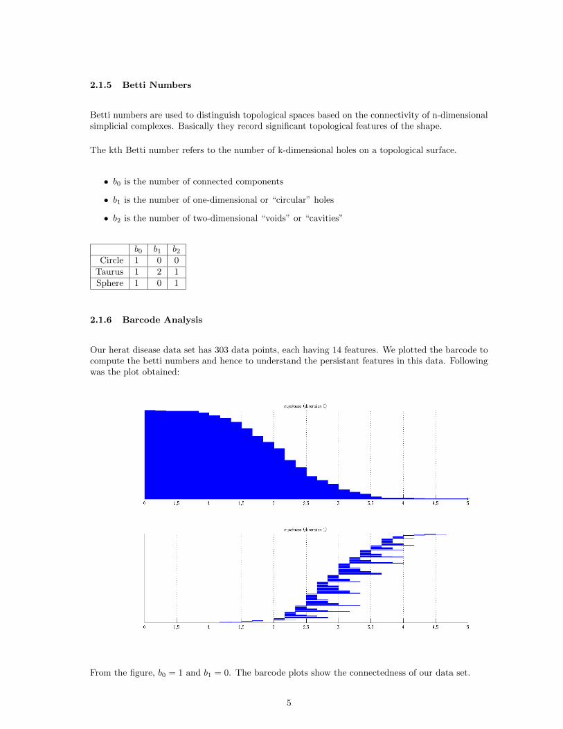
2.1.6 Barcode Analysis

Our herat disease data set has 303 data points, each having 14 features. We plotted the barcode tocompute the betti numbers and hence to understand the persistant features in this data. Followingwas the plot obtained:

From the figure, b0 = 1 and b1 = 0. The barcode plots show the connectedness of our data set.

5

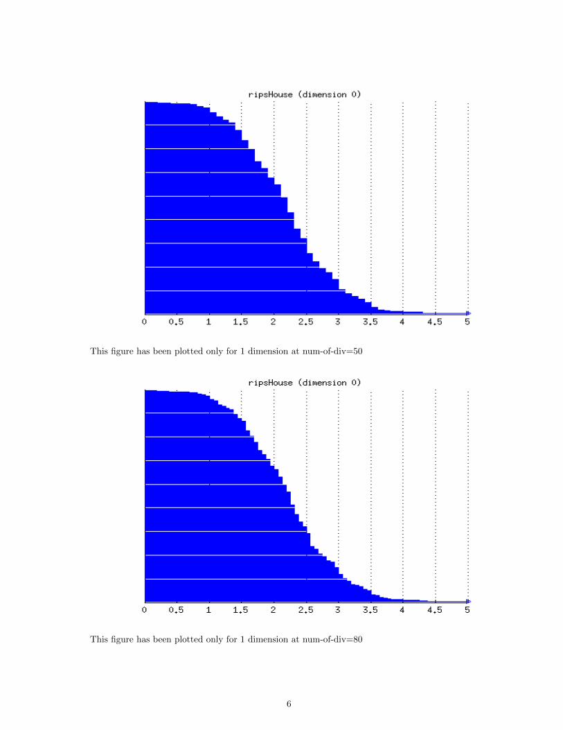
This figure has been plotted only for 1 dimension at num-of-div=50

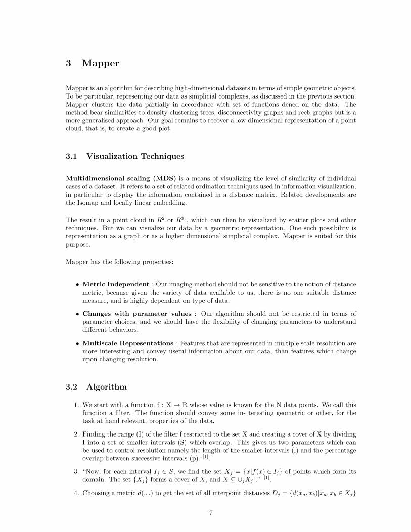
This figure has been plotted only for 1 dimension at num-of-div=80

6

3 Mapper

Mapper is an algorithm for describing high-dimensional datasets in terms of simple geometric objects.To be particular, representing our data as simplicial complexes, as discussed in the previous section.Mapper clusters the data partially in accordance with set of functions dened on the data. Themethod bear similarities to density clustering trees, disconnectivity graphs and reeb graphs but is amore generalised approach. Our goal remains to recover a low-dimensional representation of a pointcloud, that is, to create a good plot.

3.1 Visualization Techniques

Multidimensional scaling (MDS) is a means of visualizing the level of similarity of individualcases of a dataset. It refers to a set of related ordination techniques used in information visualization,in particular to display the information contained in a distance matrix. Related developments arethe Isomap and locally linear embedding.

The result in a point cloud in R2 or R3 , which can then be visualized by scatter plots and othertechniques. But we can visualize our data by a geometric representation. One such possibility isrepresentation as a graph or as a higher dimensional simplicial complex. Mapper is suited for thispurpose.

Mapper has the following properties:

• Metric Independent : Our imaging method should not be sensitive to the notion of distancemetric, because given the variety of data available to us, there is no one suitable distancemeasure, and is highly dependent on type of data.

• Changes with parameter values : Our algorithm should not be restricted in terms ofparameter choices, and we should have the flexibility of changing parameters to understanddifferent behaviors.

• Multiscale Representations : Features that are represented in multiple scale resolution aremore interesting and convey useful information about our data, than features which changeupon changing resolution.

3.2 Algorithm

1. We start with a function f : X → R whose value is known for the N data points. We call thisfunction a filter. The function should convey some in- teresting geometric or other, for thetask at hand relevant, properties of the data.

2. Finding the range (I) of the filter f restricted to the set X and creating a cover of X by dividingI into a set of smaller intervals (S) which overlap. This gives us two parameters which canbe used to control resolution namely the length of the smaller intervals (l) and the percentageoverlap between successive intervals (p). [1].

3. “Now, for each interval Ij ∈ S, we find the set Xj = {x|f(x) ∈ Ij} of points which form itsdomain. The set {Xj} forms a cover of X, and X ⊆ ∪jXj .” [1].

4. Choosing a metric d(., .) to get the set of all interpoint distances Dj = {d(xa, xb)|xa, xb ∈ Xj}

7

5. For each Xj together with the set of distances Dj we find clusters {Xjk}

6. Each cluster then becomes a vertex in our complex and an edge is created between vertices ifXjk ∩Xlm = ∅ meaning that two clusters share a common point.

3.2.1 Choices to be Made

We have to make various parameter choices whie implementing mapper function. We are listingdown the choices we made while performing analysis on heart disease data set. Our approach wasto compute using various choices and figure out the parameters that give us interesting results.

1. Choose how to cluster, and for that, we need to define a distance metric. As mentioned earlier,any measure of closeness can be chosen. We normalized our data using standard score andchose two metrics 1) Modified Euclidean Norm as a distance metric with a factor parameterfor each feature. 2) Pearson correlation cofficients.

2. Choosing our filter functionFilter function is mapping of n-dimensional data set to a lower dimesnions. e.g. f(x, y, z) → xOther possibilities :b. L∞ centralityc. Vector Norm

In our analysis, we experimented with following functions:a. L∞ centrality 1

b. On the basis of individual data features eg Age, Cholestrol.c. On the basis of distance from a given fixed node.

3. BinningPut data into overlapping bins. We have to choose the length and the percentage overlap. Wetook 25, 50 and 75 percentage overlap and number of bins to be 3, 5 and 10 as different cases.

Different choice of parameters may generate a network with a different shape and thus allowing oneto explore data from a different perspective.

We performed analysis on heart disease data set. Data set was taken from [4]

The data has 303 data points, each having 14 features.

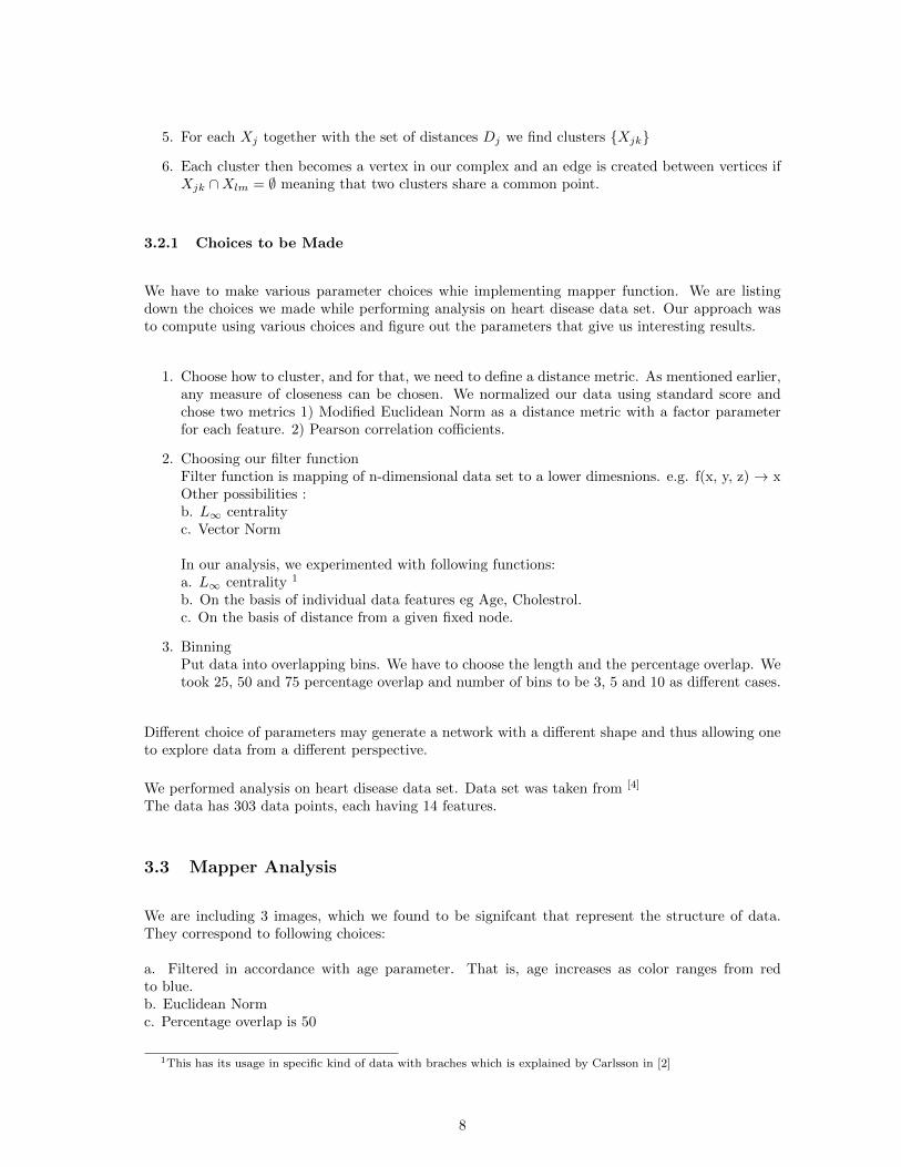
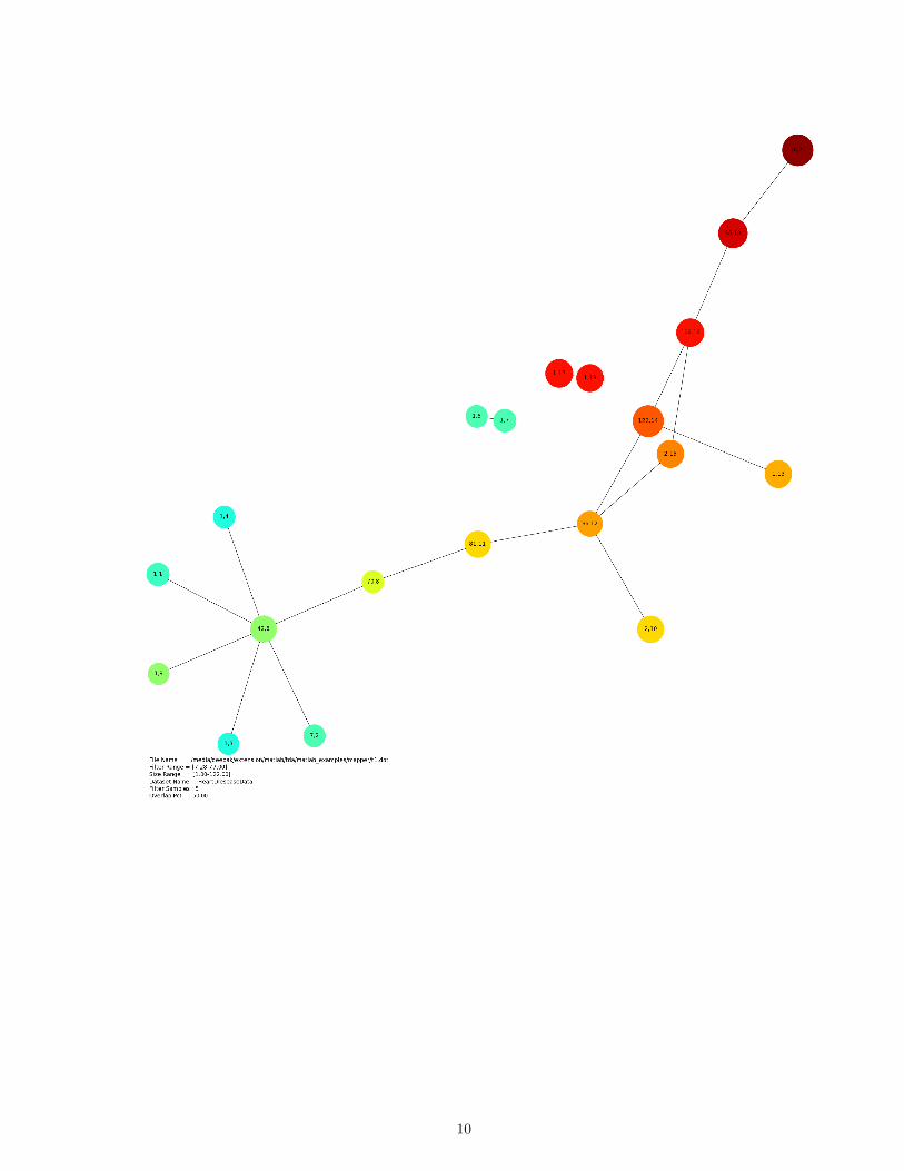
3.3 Mapper Analysis

We are including 3 images, which we found to be signifcant that represent the structure of data.They correspond to following choices:

a. Filtered in accordance with age parameter. That is, age increases as color ranges from redto blue.b. Euclidean Normc. Percentage overlap is 50

1This has its usage in specific kind of data with braches which is explained by Carlsson in [2]

8

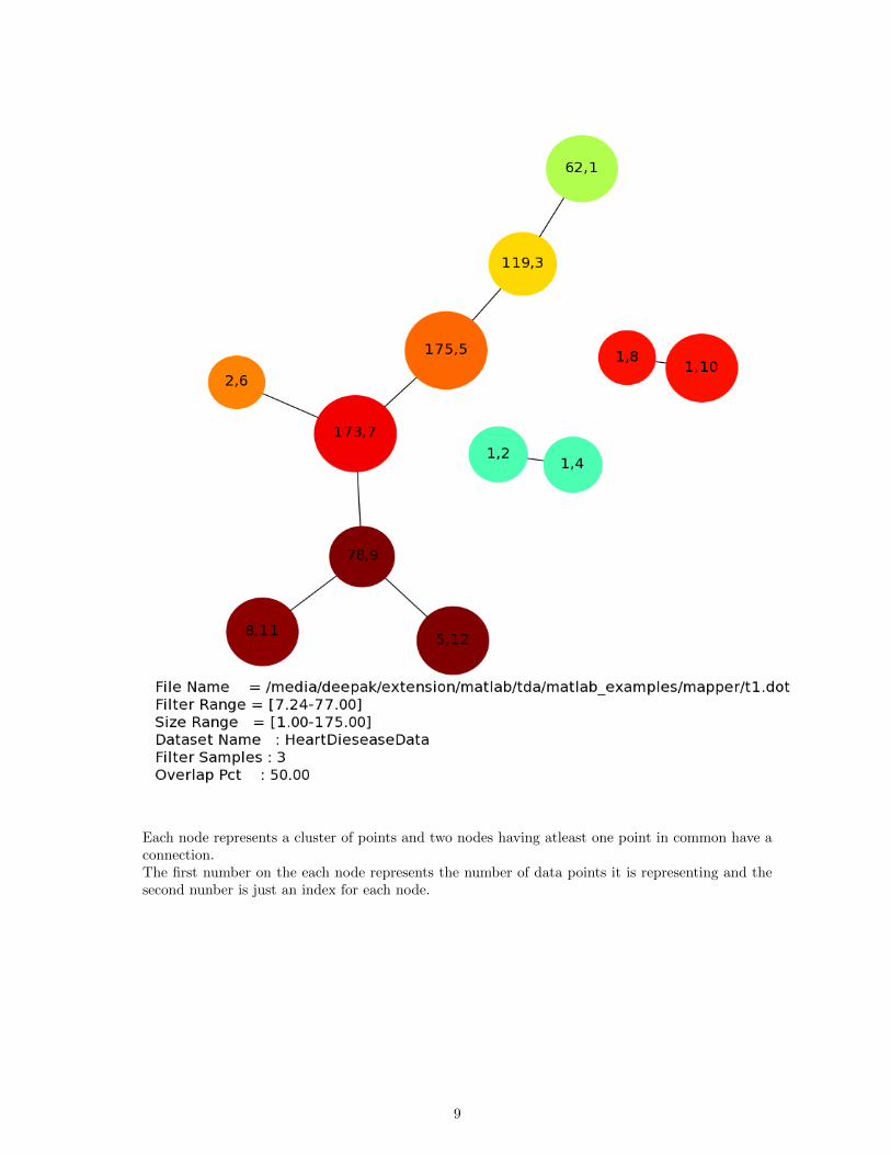
Each node represents a cluster of points and two nodes having atleast one point in common have aconnection.The first number on the each node represents the number of data points it is representing and thesecond nunber is just an index for each node.

9

10

4 Future Works

There is a lot to explore in this field. It seems that questions are many but we were able to workonly on a few. Further works are suggested below:

• We can use more variants for distance metric like modified L1 norm and cosine distance.

• Existing possibilies for even more filter functions. for eg 1) a filter function which is a linearcombination of two of more important attributes rather than just one or even a filter functionoof top 5-6 eigenvectors from PCA. 2) a density estimator filter function

• Better insights into theoritical understanding of Betti numbers(or topology) will lead to betterconclusions from barcode analysis

11

• Associate and display statistical data of each nodes on the mapper graph. In case of imagesinstead of statistical data of node rather should represent the image in small size. This wouldincrease the speed of analysis and really deepen the understanding of the mapper algorithm.Something similar on this has been shown in Carlsson’s paper [2] page 30.

• After applying mapper and getting clusters, again applying mapper on each node. This wouldbe a very nice recusive approach to understand large data sets.

• We can compare this heart disease data set to another heart disease data set from a differentsource.

5 Conclusions

5.1 Betti0

After studying betti 0 on num − of − div = 80 we see that the modulus of slope of graph is smallinitially which increases and the again decreases. This leads us to the conclusion that most pointhave distances that lie in between 1 to 3 as can be seen from betti0 figure.

6 Softwares Used

1. JavaPlex

2. Mapper (Maintained by Comptop.stanford.edu)

3. Matlab

4. Graphviz

References

[1] Gurjeet Singh, Facundo Mmoli, and Gunnar Carlsson. Topological methods for the analysis ofhigh dimensional data sets and 3d object recognition. In Eu- rographics Symposium on Point-Based Graphics, volume 22. The Eurographics Association, 2007.

[2] Gunnar Carlsson. Topology and data. Bulletin of The American Mathematical Society, January29 2009.

[3] Lum, P.Y., Singh, G., Lehman, A., Ishkanov, T., Vejdemo-Johansson, M., Alagappan, M.,Carlsson, J., Carlsson, G.: Extracting insights from the shape of complex data using topology.Sci. Rep. 3 (2013).

[4] Heart Disease Data Set, Hungarian Institute of Cardiology. Budapest: Andras Janosi, M.D.

12