The London School of Economics and Political Science

Topics in Portfolio Optimisation

and Systemic Risk

Mathieu Steve Dubois

A thesis submitted to the Department of Mathematics ofthe London School of Economics and Political Science

for the degree of

Doctor of Philosophy

London, October 2015

Declaration

I certify that the thesis I have presented for examination for the MPhil/PhD

degree of the London School of Economics and Political Science is solely my

own work other than where I have clearly indicated that it is the work of

others (in which case the extent of any work carried out jointly by me and

any other person is clearly identified in it).

The copyright of this thesis rests with the author. Quotation from it is

permitted, provided that full acknowledgement is made. This thesis may

not be reproduced without my prior written consent.

I warrant that this authorisation does not, to the best of my belief,

infringe the rights of any third party.

I declare that my thesis consists of 126 pages.

Statement of conjoint work:

I confirm that first part of the thesis was first published as a co-authored

article with my supervisor, Dr. Luitgard Veraart, in SIAM Journal on Fi-

nancial Mathematics, Vol. 6, pp. 201-241, 2015; published by the Society for

Industrial and Applied Mathematics (SIAM). Unauthorized reproduction of

this article is prohibited.

1

Abstract

This thesis is concerned with different sources of risk occurring in financial

markets. We follow a bottom-up approach by carrying out an analysis from

the perspective of a single investor to the whole banking system.

We first consider an investor who faces parameter uncertainty in a contin-

uous-time financial market. We model the investor’s preference by a power

utility function leading to constant relative risk aversion. We show that the

loss in expected utility is large when using a simple plug-in strategy for un-

known parameters. We also provide theoretical results that show the trade-

off between holding a well-diversified portfolio and a portfolio that is robust

against estimation errors. To reduce the effect of estimation, we constrain

the weights of the risky assets with a norm leading to a sparse portfolio.

We provide analytical results that show how the sparsity of the constrained

portfolio depends on the coefficient of relative risk aversion. Based on a

simulation study, we demonstrate the existence and the uniqueness of an

optimal bound on the norm for each level of relative risk aversion.

Next, we consider the interbank lending market as a network in which the

nodes represent banks and the directed edges represent interbank liabilities.

The interbank network is characterised by the matrix of liabilities whose

entries are not directly observable, as bank balance sheets provide only total

exposures to the interbank market. Using a Bayesian approach, we assume

that each entry follows a Gamma distributed prior. We then construct a

Gibbs sampler of the conditional joint distribution of interbank liabilities

given total interbank liabilities and total interbank assets. We illustrate

our methodology with a stress test on two networks of eleven and seventy-

six banks. We identify under which circumstances the choice of the prior

influences the stability and the structure of the network.

2

Acknowledgements

First and foremost I would like to thank Luitgard Veraart for the supervision

of this thesis. Her guidance and constant support have been invaluable. I

am also grateful to Jorn Sass and Mihail Zervos for readily accepting to act

as my examiners.

I would like to thank the faculty members of the Department of Mathe-

matics and the Systemic Risk Center. They provided a pleasant and stim-

ulating atmosphere to carry out academic research. Special thanks go to

the participants of the Financial Mathematics Reading Group, in particular

Christoph Czychowsky and Jose Pasos, for their thought-provoking ques-

tions that helped to grow abstract and nascent ideas into tangible concepts.

I am also grateful to Albina Danilova, Pavel Gapeev, Katja Neugebauer,

and Andreas Uthemann for generously sharing their experience of the inner

workings of the academic world.

I would also like to express my gratitude to my scholarship donors Liz

and Peter Jones. Thanks to their warm hospitality, I have got the chance to

discover English culture. Finally, I would like to thank my parents, Francoise

and Michel, and my partner, Polina. Their support and optimism have been

a driving force throughout my graduate studies.

Financial support by the Jones/Markham scholarship and the Economic

and Social Research Council [grant number ES/K002309/1] is gratefully

acknowledged.

3

Contents

1 Introduction 12

1.1 Portfolio Choice Theory and Parameter Uncertainty . . . . . 14

1.2 Systemic Risk in Financial Networks . . . . . . . . . . . . . . 16

I Optimal Diversification in Presence of Parameter Un-

certainty 19

2 The Merton Portfolio with Unknown Drift 20

2.1 Introduction . . . . . . . . . . . . . . . . . . . . . . . . . . . . 20

2.2 Model Setup . . . . . . . . . . . . . . . . . . . . . . . . . . . 24

2.2.1 The Investor’s Objective and the Classical Solution . . 25

2.2.2 The Effect of Diversification for Known Parameters . 26

2.3 Performance of Plug-in Strategies . . . . . . . . . . . . . . . . 28

2.3.1 Measures of Economic Loss . . . . . . . . . . . . . . . 31

2.3.2 Drift versus Covariance Estimation . . . . . . . . . . . 35

3 The L1-restricted Portfolio 37

3.1 Reduction to the Static Problem . . . . . . . . . . . . . . . . 37

3.2 Structure of the Optimal Strategy . . . . . . . . . . . . . . . 41

3.3 The Constrained Plug-in Strategy: Sparsity and Estimation . 47

3.4 Simulation Study . . . . . . . . . . . . . . . . . . . . . . . . . 52

3.4.1 Methodology . . . . . . . . . . . . . . . . . . . . . . . 52

3.4.2 Computation of the Loss Function . . . . . . . . . . . 53

3.4.3 Existence of an Optimal Bound . . . . . . . . . . . . . 55

3.4.4 Structure and Stability of the L1-constrained Strategy 56

4

4 Out-of-Sample Study 60

4.1 Choosing the L1-bound . . . . . . . . . . . . . . . . . . . . . 61

4.2 Performance of the Plug-in Strategies . . . . . . . . . . . . . 62

4.3 Structure and Stability of the Strategies . . . . . . . . . . . . 65

4.4 Transaction Costs . . . . . . . . . . . . . . . . . . . . . . . . 66

4.5 A Note on the Estimation of the Covariance Matrix . . . . . 69

4.6 Conclusion . . . . . . . . . . . . . . . . . . . . . . . . . . . . 69

A Proofs of Chapter 2 71

B Proofs of Chapter 3 74

C Number of Paths for the Monte-Carlo Method 76

II A Bayesian Approach to Risk Assessment in Banking

Networks 79

5 Estimation of Bilateral Exposures 80

5.1 Introduction . . . . . . . . . . . . . . . . . . . . . . . . . . . . 80

5.2 Model Setup . . . . . . . . . . . . . . . . . . . . . . . . . . . 84

5.3 The Gibbs Sampler . . . . . . . . . . . . . . . . . . . . . . . . 87

5.3.1 Conditional Distribution . . . . . . . . . . . . . . . . . 88

5.3.2 Sampling from the Conditional Distribution . . . . . . 92

6 Empirical Example 96

6.1 Stress Test Setup . . . . . . . . . . . . . . . . . . . . . . . . . 96

6.1.1 Balance Sheet Contagion Model . . . . . . . . . . . . 96

6.1.2 Choice of the Parameters . . . . . . . . . . . . . . . . 99

6.2 Small Network . . . . . . . . . . . . . . . . . . . . . . . . . . 102

6.2.1 Properties of the Conditional Distribution . . . . . . . 102

6.2.2 Stress Test . . . . . . . . . . . . . . . . . . . . . . . . 105

6.2.3 Structure of the Small Network . . . . . . . . . . . . . 107

6.3 Large Network . . . . . . . . . . . . . . . . . . . . . . . . . . 108

6.3.1 Stress test . . . . . . . . . . . . . . . . . . . . . . . . . 108

6.3.2 Structure of the Large Network . . . . . . . . . . . . . 110

6.4 Conclusion . . . . . . . . . . . . . . . . . . . . . . . . . . . . 110

5

D Balance Sheet: German Network 116

E Balance Sheet: European Network 117

6

List of Figures

2.1 Plot of the efficiency of the plug-in investor relative to the

Merton investor as a function of the number of risky assets

d for different levels of risk aversion γ. For a given γ, the

efficiency depends only the number of risky assets, the in-

vestment horizon T = 1 and the observation period tobs = 10. 35

3.1 Plot of the log-loss factor due to under-diversification `γ (π∗c , π∗),

due to estimation `γ (πc, π∗c ) and the total loss factor `γ (πc, π

∗)

as a function of the bound of the L1-constraint c with γ = 5. 55

3.2 Number of stocks invested in as a function of the bound c of

the L1-constraint for different RRA coefficients γ. We have

chosen r = 0.02 for the annual risk-free rate. . . . . . . . . . 57

5.1 Illustration of submatrices for cycles of size k = 2, 3, 4; see

Gandy and Veraart (2015) Figure 1. . . . . . . . . . . . . . . 87

6.1 Plot of the continuous part of the density of the random vari-

able ∆ on two cycles of different sizes. The cycles are chosen

such that the support of ∆ is the same on both cycles. Pa-

rameters: Sample size = 10000, edge probability p = 0.5,

shape parameter α = 1 (full), α = 3 (dashed) and α = 5

(dashed/dotted). . . . . . . . . . . . . . . . . . . . . . . . . . 102

6.2 Plot of the continuous part of the density of liabilities L13 and

L31 for different values of the shape parameter α.Parameters:

Sample size = 10000, edge probability p = 0.5, α = 2 (full) ,

α = 3.5 (dashed), α = 5. (dashed/dotted). . . . . . . . . . . . 104

7

6.3 Plot of the probability of default, without cost (first column)

and with default costs (second column), as a function of the

edge probability p for different values of shape parameters.

Bank DE019 (dotted), DE020 (full), DE025 (dashed), DE028

(dashed/dotted). Parameters: Sample size = 10000, external

shock, s = 0.97, default costs d = 0.95. . . . . . . . . . . . . . 112

6.4 Plot of the mean out-degree of bank j, E(∑

j Aij |a, l), as

a function of the edge probability p for different values of

shape parameters. Parameters: Sample size = 10000, exter-

nal shock, s = 0.97, default costs d = 0.95. . . . . . . . . . . 113

6.5 Plot of the probability of default, without cost (first column)

and with default costs (second column), as a function of the

edge probability p for different values of shape parameters.

Parameters: Sample size = 10000, external shock, s = 0.96,

default costs d = 0.96. Bank ES067 (full), ES076 (dashed),

IE039 (dashed/dotted). . . . . . . . . . . . . . . . . . . . . . 114

6.6 Plot of the mean out-degree of bank j, E(∑

j Aij |a, l), as

a function of the edge probability p for different values of

shape parameters. Parameters: Sample size = 10000, exter-

nal shock, s = 0.96, default costs d = 0.96. . . . . . . . . . . . 115

E.1 Balance sheet information of 76 European banks system for

the 2011 EBA stress test. The data is provided in Glasserman

and Young (2015). All quantities are in million euros. . . . . 119

8

List of Tables

3.1 Comparison of the log-loss in expected utility and the effi-

ciency between the constrained and the unconstrained case,

for different values of risk aversion γ. The log-loss factor is

equal to zero when there is no loss. . . . . . . . . . . . . . . . 55

3.2 Characteristics of the 21 stocks selected for the constrained

strategy π∗c with known parameters. The first column corre-

sponds to the general index of stock i. The second columns

corresponds to the global rank in term of excess returns. The

third column shows the associated excess return. The fourth

and the fifth columns report the weights. Parameters: Bound

of the L1-constraint c = 3, coefficient of RRA γ = 2, annual

risk-free rate r = 0.02. . . . . . . . . . . . . . . . . . . . . . . 58

3.3 This table reports the expected value (and standard devia-

tion) of the number of stocks invested in, the number of shorts

positions, the fraction in L1-norm of short positions and the

average of the standard deviation of the weights. The quan-

tities presented are the sample mean and standard deviation

over M = 5000 realisations. The optimal bound c of the

L1-constrained strategy is chosen as in Table 3.1. The un-

constrained Merton plug-in strategy corresponds to c = ∞.

Parameters: Coefficient of RRA γ = 2, annual risk-free rate

r = 0.02. . . . . . . . . . . . . . . . . . . . . . . . . . . . . . . 59

4.1 This table reports the summary statistics of the optimal bounds

c for the leave-one-block out (LOB) and the cross validation

(CV) methods for the three time periods that we consider.

Parameters: Coefficient of RRA γ = 2, investment horizon

T = 1/12, and annual risk-free rate r = 0.02 . . . . . . . . . 62

9

4.2 This table reports the summary statistics of the utility and

the monthly returns of final wealth out-of-sample. The quan-

tities presented are computed over each block of 24 months.

The optimal bounds c of the L1-constrained strategies are cal-

ibrated using the leave-one-block-out (LOB) and the cross-

validation (CV) methods. Parameters: Coefficient of RRA

γ = 2, initial wealth XM (0) = 1, investment horizon T =

1/12, and annual risk-free rate r = 0.02. . . . . . . . . . . . . 64

4.3 This table reports the mean value (standard deviation) of the

number of stocks invested in, of the number of shorts posi-

tions, of the fraction in L1-norm of short positions, and the

mean monthly turnover for four different investment strate-

gies. The mean is computed over each block of 24 months.

The optimal bound c of the L1-constrained strategy is cal-

ibrated with the leave-one-block out (LOB) and the cross

validation (CV) methods. Parameters: Coefficient of RRA

γ = 2, investment horizon T = 1/12, and annual risk-free

rate r = 0.02. . . . . . . . . . . . . . . . . . . . . . . . . . . . 67

4.4 This table reports the minimum, mean and maximum of util-

ity of terminal wealth averaged over 24 months for three time

periods. Four different strategies are considered: The uncon-

strained plug-in strategy using (3.4.1) and (3.4.2), denoted by

unconst, unconstrained plug-in strategy using (3.4.1) and the

method proposed by Ledoit and Wolf (2004a) for the covari-

ance matrix, denoted by unconst, L&W, and the correspond-

ing strategies where we imposed an L1-constraint, denoted by

L1 and L1, L&W, respectively. . . . . . . . . . . . . . . . . . 70

10

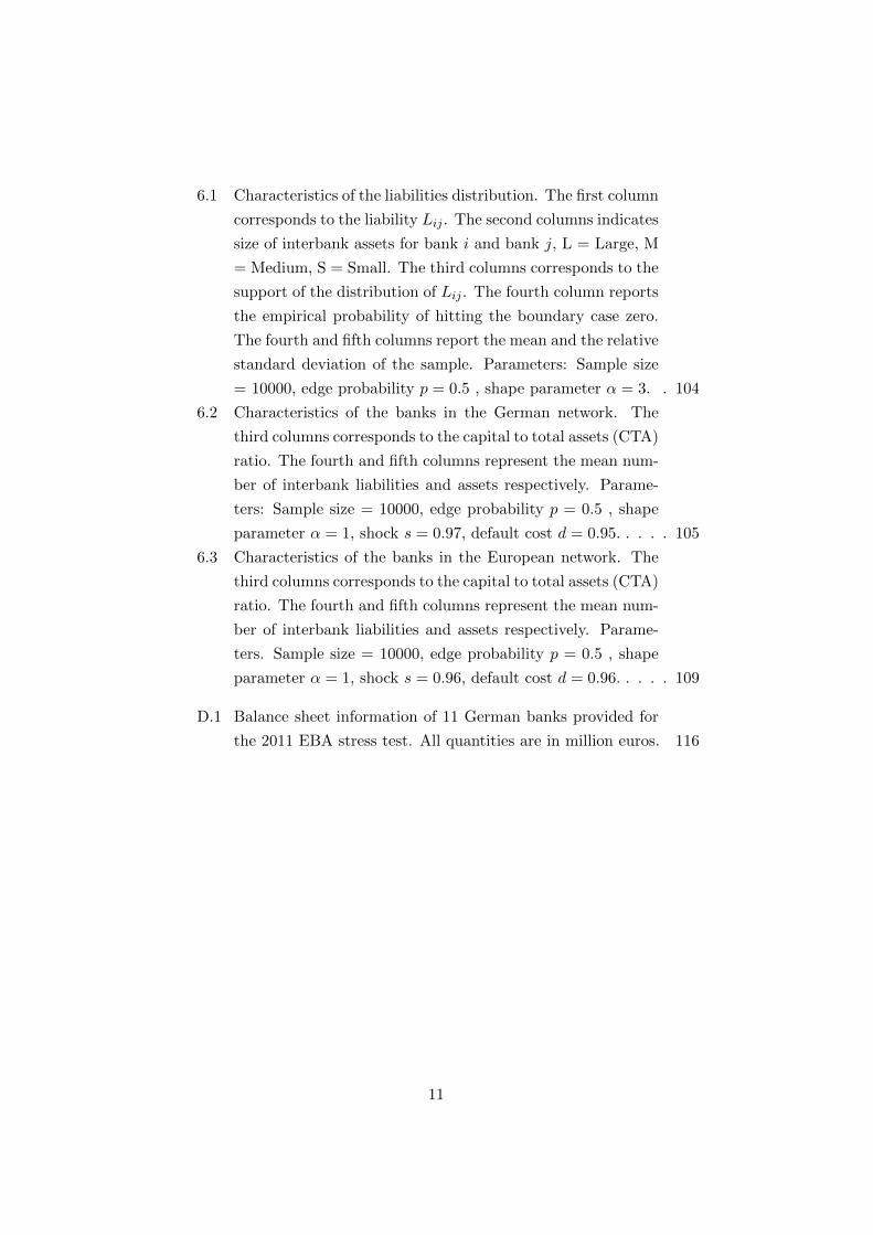
6.1 Characteristics of the liabilities distribution. The first column

corresponds to the liability Lij . The second columns indicates

size of interbank assets for bank i and bank j, L = Large, M

= Medium, S = Small. The third columns corresponds to the

support of the distribution of Lij . The fourth column reports

the empirical probability of hitting the boundary case zero.

The fourth and fifth columns report the mean and the relative

standard deviation of the sample. Parameters: Sample size

= 10000, edge probability p = 0.5 , shape parameter α = 3. . 104

6.2 Characteristics of the banks in the German network. The

third columns corresponds to the capital to total assets (CTA)

ratio. The fourth and fifth columns represent the mean num-

ber of interbank liabilities and assets respectively. Parame-

ters: Sample size = 10000, edge probability p = 0.5 , shape

parameter α = 1, shock s = 0.97, default cost d = 0.95. . . . . 105

6.3 Characteristics of the banks in the European network. The

third columns corresponds to the capital to total assets (CTA)

ratio. The fourth and fifth columns represent the mean num-

ber of interbank liabilities and assets respectively. Parame-

ters. Sample size = 10000, edge probability p = 0.5 , shape

parameter α = 1, shock s = 0.96, default cost d = 0.96. . . . . 109

D.1 Balance sheet information of 11 German banks provided for

the 2011 EBA stress test. All quantities are in million euros. 116

11

Chapter 1

Introduction

One should always divide his wealth into three parts: a third

in land, a third in merchandise, and a third ready to hand.

- Babylonian Talmud: Tractate Baba Mezi’a, 3rd to 5th century A.D.

As the quote above suggests, the problem of wealth allocation through di-

versification is a long standing concern. The first methodological framework

for a mathematical formulation of diversification is developed in Markowitz

(1952). In his seminal article, he assumes that investors care about mean

returns and consider variance as “an undesirable thing”, (Markowitz, 1952,

p. 77). He then shows that the risk specific to each asset, also called idiosyn-

cratic risk, can be eliminated through diversification by taking advantage of

the imperfect correlation between assets. Finally, he identifies the portfolio

with maximal mean return for a given level of variance. By allowing the

variance to vary, the set of optimal portfolios (the efficient frontier) is ob-

tained. Every portfolio below the efficient frontier is suboptimal and can be

further diversified, while the region above the frontier is simply unattainable

with the given universe of risky assets.

The mean-variance approach has had a profound impact in financial eco-

nomics and research in modern portfolio theory has focused on understand-

ing its limitations and improving on it. This framework implicitly assumes

that the financial market is granular so that the interactions between ac-

tors are not relevant. The systemic risk literature takes a complementary

approach by studying when and how the stability of the financial market

is affected by the structure of exposures among banks. Therefore, from a

12

systemic perspective, the diversification of exposures is a determinant factor

of stability.

This thesis investigates different sources of risk faced by individual in-

vestors and financial institutions. In the first part of the thesis, we study

the performance of a standard dynamic model-based investment strategy

for investors facing parameter uncertainty. To control the effect of estima-

tion, we constrain the proportion of wealth invested in risky assets with

a suitable norm leading to a sparse portfolio. We present novel analytical

results that show how the sparsity of the constrained portfolio depends on

the investor’s risk aversion. Our work contributes to the portfolio theory

literature by identifying an optimal degree of diversification with respect to

the estimation procedure and the investor’s preferences. We build a sparse

dynamic strategy that is robust against estimation errors for each risk averse

investor. We then show that the optimally constrained strategy performs

well out-of-sample.

In the second part of the thesis, we model the interbank lending market

as a network in which nodes represent banks and directed edges represent

interbank liabilities. The network is then characterised by the matrix of

liabilities whose entries are not directly observable, as a bank balance sheet

provides only its total of interbank liabilities (sum of rows) and its total

interbank assets (sum of columns).

Using a Bayesian approach, we assume that each entry follows a specific

prior distribution. We then develop a novel numerical method to sample

from the conditional joint distribution of interbank liabilities given total

interbank liabilities and total interbank assets. Our methodology allows us

to carry out stress tests. Our results establish under which circumstances

the choice of the prior distribution has an influence both on the structure

and the stability of the interbank market.

In the rest of this chapter, we review the literature on estimation risk in

portfolio theory and systemic risk. Through this historical perspective, we

aim to convince the reader that diversification is a powerful, yet delicate,

tool to manage both sources of risk.

13

1.1 Portfolio Choice Theory and Parameter Un-

certainty

The implementation of a portfolio, based on a model of risk and return, re-

quires the estimation of expected returns, variance and correlation between

assets, as these quantities are not directly observed. Parameter uncertainty

is a major source of risk since strategies based on naive estimation meth-

ods are known to perform poorly. In portfolio theory, there are two differ-

ent econometric approaches to treat the problem of parameter uncertainty,

namely decision theory and plug-in estimation. In the decision theory ap-

proach, each parameter has a prior distribution and uncertainty about these

parameters is included in the objective function of the optimisation problem;

see Brandt (2010) for a review of the literature on decision theory applied

to portfolio choice problems. Therefore, the portfolio rule is optimal with

respect to the prior beliefs of the investor.

In this section, we review the literature on plug-in estimation as the

method developed in the first part of the thesis is based on a plug-in estima-

tor. In the plug-in estimation approach, the estimators of the parameters,

obtained through frequentist or Bayesian inference, are simply plugged in

the expression of the optimal portfolio weights. The poor performance of

plug-in mean-variance efficient strategies has been largely documented; see,

e.g., Jobson and Korkie (1980), Michaud (1989) and Best and Grauer (1991).

In particular, the mean-variance portfolio tends to magnify the effect of esti-

mation errors by allocating extreme weights to assets whose parameters are

the least accurately estimated. Moreover, the problem worsens as the num-

ber of risky assets increases. As a result, investors should hold positions that

are untenable under real conditions. Note that a dynamic continuous-time

framework raises the same difficulties since part of the portfolio corresponds

to the mean-variance efficient term; see Merton (1971).

Three methods have been developed to control the effect of estimation

error. They all aim at avoiding the presence of extreme weights in the

portfolio to maintain a more uniform repartition of wealth across assets.

Following the shrinkage estimation procedure of James and Stein (1961),

the first method consists in shrinking the mean to a common value; see

Jobson and Korkie (1981) and Jorion (1986). Shrinkage can also be applied

to the covariance matrix, for example towards the identity matrix as in

14

Ledoit and Wolf (2004b), or directly on the portfolio weights, for example

towards an equally-weighted portfolio.

The second method imposes a factor structure on the covaration of asset

returns to reduce the number of elements to be estimated in the covariance

matrix; see the review of Fan et al. (2012). The factors can be identi-

fied through an equilibrium model such the Capital Asset Pricing Model of

Sharpe (1964), the Intertemporal Capital Asset Pricing Model of Merton

(1973), on firm characteristics as in Fama and French (1993), or through

a factor analysis; see, e.g., Roll and Ross (1980). In a minimum-variance

framework, Chan et al. (1999) show that estimation of the covariance ma-

trix with factors models improves the performance of plug-in strategies.

However, they demonstrate that no factor model stands out significantly.

Therefore, the identification, the selection, as well as the interpretation, of

the factors to be used is still an open debate.

The third method consists in adding constraints to the optimisation

problem; see, e.g., Frost and Savarino (1988) and Chopra (1993). Although

practitioners are attracted by naive “talmudic” diversification and conser-

vative constraints, such as the no-short sale constraint, Green and Holli-

field (1992) show that optimally diversified portfolios may include extreme

weights to reduce systematic risk. As such, controlling estimation risk by

adding constraints is not necessarily justified from a theoretical perspec-

tive. Jagannathan and Ma (2003) resolve this conflict, between theory and

traditional asset management practices, by showing that the no-short sale

constraint is a shrinkage procedure. Indeed, imposing a no-short sale con-

straint is tantamount to shrink towards zero large elements of the covariance

matrix estimator. Consequently, the associated portfolio is sparse. While

excluding assets from the investment rule inherently reduces the effect of

estimation error, the exposure to idiosyncratic risk is increased. In particu-

lar, DeMiguel et al. (2009a) show that no-short sale constrained portfolios,

as well as none of the approaches mentioned above, are able to beat consis-

tently an equally-weighted portfolio. As such, a series of articles relax the

no-short sale constraint to the L1-constraint, which controls the percentage

of short positions held in the portfolio; see DeMiguel et al. (2009a), Brodie

et al. (2009) and Fan et al. (2012). This constraint also induces sparsity in

the portfolio, hence reducing estimation risk. The resulting portfolio outper-

forms out-of-sample the no-short sale constrained and the equally-weighted

15

portfolios in terms of Sharpe ratio.

Because the estimation error in the sample mean is large when based

on historical returns, mean-variance portfolios usually perform worse out-

of-sample than minimun-variance portfolios. Hence, the main focus of the

literature, that we have reviewed, is on the estimation of the covariance

matrix. However, the mean-variance criterion applies only if returns are

normal or the investor has a quadratic utility. Otherwise, for general util-

ity functions in a market with non-normal returns, the portfolio is only an

approximation of the true optimal one; see Levy and Markowitz (1979).

Therefore, the development of methods that take into account the estima-

tion of mean returns, and deliver a stable out-of-sample performance, still

challenges researchers in applied portfolio theory.

1.2 Systemic Risk in Financial Networks

Although there is not a full agreement on the definition of systemic risk in the

academic community, we define it as the risk of an external shock spreading

to the entire financial network through different channels of endogenous

risk1. We list here three main channels of systemic risk; for a complete

survey, see De Bandt et al. (2009) and Benoit et al. (2015). The first channel

is that financial institutions are exposed to similar risk by investing in highly

correlated assets; see Haldane (2009). As there is not enough diversification

in portfolios at a systemic level, banks fail together. This behaviour can be

nonetheless optimal from the banks perspective. For example, Acharya and

Yorulmazer (2008) show that banks maximize their profit by failing together

as it ensures a common bail-out from the government. Similarly Farhi and

Tirole (2012) argue that bail-outs are optimal when the entire system fails,

since any bail-out has a fixed cost for the government.

The second channel is liquidity contagion. Liquidity crises are driven

by an amplification mechanism which can be decomposed into a loss spiral

and a margin spiral; see Brunnermeier and Oehmke (2013). The loss spiral

arises as levered financial institutions are very sensitive to a fall in value of

their total assets so that they are forced to liquidate their assets at the same

time to reach their respective regulatory leverage ratios. This increased

1This definition applies to 205 papers, over the past 35 years, surveyed in Benoit et al.(2015)

16

pressure leads to fire sales, i.e. assets are traded with a discount. Then a

margin spiral arises as fire sales are a signal for higher volatility in which case

creditors require higher margins amplifying the volatility. Hence, financial

institutions are trapped into two contagious spirals reinforcing each other.

The third channel is default contagion, which can be thought of as a

domino effect. In the case of an external shock, the default of one bank

leads to a reduction of expected payments to other banks. If such banks are

too exposed to the interbank market, or their assets are also significantly

reduced by the external shock, they will not be able to cover their losses

and they will also default. The spread of balance sheet contagion depends

fundamentally on the diversification of banks’ bilateral exposures. Under

different modeling assumptions, Allen and Gale (2000) and Freixas et al.

(2000) show that a complete network in which all banks are connected is less

prone to contagion than a network in which banks are minimally connected

in a circular credit chain fashion. Moreover, in Freixas et al. (2000), a large

enough number of banks ensures the stability of a complete network, while

the number of banks has no effect on the stability of a circular network.

Based on the Erdos and Renyi (1959) random graph model, in which

banks are exposed to each other with a fixed probability, Nier et al. (2007)

use simulations to highlight patterns affecting the stability of the network.

In particular, their results demonstrate that there is a non monotonic M-

shaped relation between the number of defaults and the number of interbank

connections. They also identify additional parameters such as the capital-

isation of banks, the size of exposures to the lending interbank network as

well their concentration as determinant factors for the stability of the in-

terbank lending market. Note that the three articles cited above assume

that the default contagion is triggered by an exogeneous idiosyncratic shock

on a single bank. This assumption is not likely to provide a full picture of

the network stability in times of crises as several institutions are affected

simultaneously. In a recent article, Acemoglu et al. (2015) actually show

that the capacity of a complete network to absorb defaults depends on the

size and the number of shocks applied to the system.

Based on data of national banking systems, a significant number of em-

pirical papers has been published; see, e.g., Furfine (2003) for the United

States, Wells (2004) for Germany, Elsinger et al. (2006) for the UK, Van

and Liedorp (2006) for the Netherlands, Degryse and Nguyen (2007) for

17

Belgium. They analyse the stability of the respective networks through dif-

ferent methods of stress test and these papers establish that contagion due

interbank lending is limited. Nevertheless, Upper (2011) argues that no clear

cut conclusions can be made from these studies given the difference of net-

work structure across countries as well as the variety of simulation methods.

Moreover, he identifies two main methodological drawbacks on which most

of the studies rely. Similarly to the early theoretical literature, only balance

sheet contagion triggered by a single default is analysed. Next, because of

the censorship of individual banks’ exposures in most countries, the stress

tests require an estimation of the actual network. The construction of the

network relies on minimising the Kullback-Leibler divergence with respect

to a prior network in which liabilities are evenly distributed. The network

obtained through this method is complete in the sense of Allen and Gale

(2000) and it is a feature at odds with fully observable networks; see Upper

and Worms (2004), Cocco et al. (2009), and Cont et al. (2013). Indeed,

observed networks are usually sparse and have a core periphery structure.

To answer the need of an estimation method providing a more realistic

network structure, Gandy and Veraart (2015) develop a Bayesian approach

in which each exposure follows an exponential prior conditionally on a prior

probability of existence. Using a Markov Chain Monte Carlo method, they

draw samples from the joint distribution of the individual liabilities condi-

tionally on the information provided by balance sheets. Their model allows

for full heterogeneity in the parameters and also for tiered network struc-

tures.

18

Part I

Optimal Diversification in

Presence of Parameter

Uncertainty

19

Chapter 2

The Merton Portfolio with

Unknown Drift

The first myth is that this research is only about how to “beat

the market”.

- Ioannis Karatzas and Steven E. Shreve, Methods of Mathematical Finance

2.1 Introduction

We consider a financial market consisting of one risk-free asset and a large

number of risky assets following a multi-dimensional geometric Brownian

motion. In this market, we assume that there is an investor with a power

utility function seeking to maximise the expected utility of her final wealth.

If all parameters are known, Merton (1971) shows that the optimal fraction

of wealth allocated in each risky asset is characterised by the drift and the

volatility matrix of assets returns1.

These two quantities are not directly observable, and they are typically

replaced by estimates computed from historical data2. For instance, we

can plug simple estimators, such as the sample or the maximum likelihood

estimators, into the analytical expression of the optimal portfolio weights.

1 When all parameters are known, Merton (1971) shows that the utility maximisationproblem is reduced to a mean-variance problem.

2It is also possible to use estimates of the covariance matrix, or equivalently the volatil-ity matrix, based on forward-looking information; see the recent work of Kempf et al.(2015) for a successful application in portfolio selection.

20

However, the resulting plug-in strategy is likely to differ considerably from

the true optimal strategy. The main source of error comes from the estima-

tion of the drift. Indeed, the accuracy of the estimator of the drift does not

depend on the frequency of observations but on the length of the observa-

tion interval. To obtain a reasonable precision for estimators of the drift,

one needs to use a very long period of observation; see Merton (1980).

Moreover, when the number of risky assets is large, the problem becomes

even more prominent as estimation errors accumulate across the positions

in the risky assets. Based on Merton (1971) and restricted to a logarithmic

utility function, Gandy and Veraart (2013) show that the expected utility

associated with the plug-in strategy can degenerate to −∞ as the number

of assets increases3 .

In this chapter, we extend the approach of Gandy and Veraart (2013)

to general power utility functions. By taking into account the coefficient of

relative risk aversion (RRA) explicitly, we are able to pin down the influence

of both risk aversion and estimation risk on the expected utility.

Next, we impose an L1-constraint on the portfolio weights. This con-

straint induces sparsity in the portfolio, i.e., most of the weights are set to

zero, and it naturally reduces the accumulation of estimation error. Our

objective is to select the bound of the L1-constraint which gives the optimal

degree of sparsity in the portfolio.

Holding a sparse portfolio is known to be an efficient way to reduce

exposure to estimation risk4. In a minimum-variance framework with a

large number of risky assets (500 stocks), Jagannathan and Ma (2003) show

that the no-short sale constraint is likely to improve the performance of the

plug-in strategy based on the sample covariance matrix. In this case, the

estimation error is large, and constraining the amount of short positions

can help because the associated plug-in strategy is sparse. However, they

also demonstrate that the portfolio has too many weights set to zero. As a

3In the static framework it is well known that plug-in mean-variance efficient portfoliosperform poorly out-of-sample. In particular, no standard plug-in strategy, outperformsconsistently the equally-weighted portfolio benchmark in terms of Sharpe ratio, certaintyequivalence, and turnover; see DeMiguel et al. (2009b) and references therein.

4Sparsity could also be induced by considering an optimal subset of available assets,i.e., by solving an L0-norm problem. Even with a quadratic objective, this is a NP-hardproblem; see Natarajan (1995) and Bach et al. (2010). In the portfolio selection literature,simple convex constraints such as L1-constraints inducing sparsity are favored because oftheir computational tractability.

21

result, the poor performance of only a few assets can dramatically influence

the performance of the portfolio.

To overcome this problem DeMiguel et al. (2009a), Brodie et al. (2009)

and Fan et al. (2012) generalise the no-short sale constraint to the less re-

strictive L1-constraint. The L1-constraint is more flexible because it imposes

an upper bound on the proportion of short positions. Thus, the set of ad-

missible portfolios is augmented by relaxing the constraint while keeping a

reasonable sparsity. With a suitable bound the constrained plug-in strategy

has a smaller out-of-sample variance than benchmark portfolios such as the

no-short sale minimum variance portfolio and the equally-weighted portfo-

lio; see DeMiguel et al. (2009a), Brodie et al. (2009) and Fan et al. (2012).

Moreover, it also outperforms strategies based on James-Stein estimators in

the static framework of DeMiguel et al. (2009a) and in the dynamic frame-

work of Gandy and Veraart (2013).

The identification of a good bound for the L1-constraint is decisive for

the performance of the constrained plug-in strategy. The empirical results

of Fan et al. (2012) demonstrate that the out-of-sample variance of the con-

strained minimum-variance plug-in strategy is convex in the bound of the

L1-constraint. In particular, the variance can be reduced by half by mov-

ing from the no-short sale constraint to the optimal L1-constraint. Relax-

ing the constraint further increases the variance up to twenty-five percent.

Therefore, a relatively small interval has to be identified for the bound.

Alternatively, DeMiguel et al. (2009a) suggest to select the bound, which

minimises the variance, using the cross-validation method. None of these

papers characterise the structure of the constrained strategy nor do they jus-

tify explicitly the existence of an optimal bound. We address these problems

as outlined below.

In Section 2.2, we introduce the general setup and recall the optimal

investment strategies when parameters are assumed to be observable. We

then drop the observability assumption of the drift in Section 2.3. We es-

timate the drift vector with the maximum likelihood estimator (MLE) and

we assume the volatility matrix to be known. This assumption is justified

by assuming that prices are observed continuously and hence the volatility

is directly observable from the quadratic variation of the logarithmic asset

price but the drift is not.

In Section 2.3, Theorem 2.3.2, we show that the expected utility of the

22

plug-in strategy is equal to the theoretical expected utility of the optimal

strategy with known parameters times a loss factor. For a fixed investment

horizon, this loss factor is increasing in the number of risky assets. In

particular, the expected utility can degenerate as the number of risky assets

increases. When the drift is estimated, the diversification of the plug-in

strategy clearly hurts.

In Section 3.1, we introduce the L1-norm as a way to constrain in-

vestment weights. We demonstrate that the sparsity of the optimal L1-

constrained strategy depends to a large extent on the coefficient of RRA.

To understand the relation between the structure of the constrained strat-

egy and the coefficient of RRA, we provide the analytical solution of the

optimal L1-constrained portfolio for independent risky assets in Theorem

3.2.2. In this case only the assets with the largest absolute excess returns

are selected. The L1-constrained portfolio rule consists in shrinking the ex-

cess returns towards zero by an intensity which is the same for all assets.

If the absolute excess return of an asset is smaller than this constant, we

do not invest in it. The number of assets invested in and the shrinkage in-

tensity depend both on the bound of the L1-constraint and the level of risk

aversion. The L1-constrained strategy becomes less sparse as the coefficient

of RRA increases, both for the true and the estimated drift. In terms of

diversification, increasing the coefficient of RRA is similar to relaxing the

constraint.

When facing parameter uncertainty, we show, in Proposition 3.3.2, that

imposing an L1-constraint rules-out degeneracy of the expected utility of

the plug-in strategy. Indeed, even if the number of assets goes to infinity,

the L1-constrained portfolio remains sparse, which prevents accumulation

of estimation error.

With a fixed number of assets, the key point is to analyse the trade-off

between the loss due to the lack of diversification, introduced by the L1-

constraint, and the loss due to estimation error. As we relax the constraint,

the loss due to under-diversification decreases, while the loss due to esti-

mation increases. These two losses move in opposite directions. Depending

on the structure of the drift, the volatility matrix, and the method of es-

timation, there can be an L1-bound which minimises the total loss of the

constrained plug-in strategy for each level of risk aversion.

For a general volatility matrix, we do not have closed form results for

23

optimal L1-constrained strategies. Therefore we use in Section 3.4 a sim-

ulation study to investigate the properties and the performance of the L1-

constrained portfolio, when assets are correlated. Similarly to the indepen-

dent case, the L1-constrained strategy becomes less sparse as the coefficient

of RRA increases. We present numerical examples which show that the

L1-bound can be chosen in an optimal way to minimise the loss due to esti-

mation. This optimal choice depends crucially on the level of risk aversion.

Finally, in Chapter 4, we consider a universe of stocks based on the S&P

500 from 2006 to 2011 and we investigate the out-of-sample performance of

the unconstrained and the constrained plug-in strategies. We trade daily

over one-month-long intervals to test the strategies. We calibrate the op-

timal bound of the constrained strategy based on two different numerical

methods. Our results confirm that the unconstrained strategy has very

unstable returns. We also demonstrate that imposing the appropriate L1-

constraint improves greatly the performance of the plug-in strategy. While,

on average, the constrained strategy has a higher variance than the equally-

weighted portfolio, it delivers a utility of terminal wealth which is in the

same range. Hence, the L1-constrained plug-in strategy has a comparable

performance to the equally-weighted portfolio, even when the drift is esti-

mated.

2.2 Model Setup

We consider a financial market where trading takes place continuously over

a finite time interval [0, T ] for 0 < T < ∞. The market consists of one

risk-free asset with time-t price S0 (t) and d risky assets with time-t price

Si (t) for i = 1, . . . , d. Their dynamics are given by

dS0 (t) = S0 (t) rdt, S0 (0) = 1,

dSi (t) = Si (t)

µidt+

d∑

j=1

σijdWj (t)

, Si (0) > 0, for i = 1, . . . , d,

where r ≥ 0 is the constant interest rate, µ = (µ1, . . . , µd)> is the constant

drift and σ = (σij)1≤i,j≤d is the constant d×d volatility matrix. We assume

that σ is of full rank. Furthermore, W = (W1, . . . ,Wd)> is a standard

d-dimensional Brownian motion on the probability space (Ω,F ,P).

24

We denote by Xπ (t) the investor’s wealth at time t when using strategy

π, which is given by

dXπ (t) =

d∑

i=0

πi (t)Xπ (t)dSi (t)

Si (t),

for a constant initial wealth Xπ (0) = X (0) > 0. Here, πi (t) denotes the

fraction of wealth invested in the ith asset at time t. Hence,∑d

i=0 πi (t) = 1

for all t. Using π0 (t) = 1−∑di=1 πi (t) and setting π (t) = (π1 (t) , . . . , πd (t))>,

we obtain

dXπ (t)

Xπ (t)=(r + π (t)> (µ− r1)

)dt+ π> (t)σdW (t) ,(2.2.1)

where 1 = (1, . . . , 1)> ∈ Rd. For strategies (π (t))t≥0 that are adapted to the

filtration (F (t))t≥0 with F (t) = σ (W (s) , s ≤ t) and that are sufficiently

integrable, the solution of (2.2.1) is

Xπ (T ) = X (0) exp

(∫ T

0

(r + π (t)> (µ− r1)− 1

2π (t)>Σπ (t)

)dt

+

∫ T

0π (t)> σdW (t)

),

where Σ = σσ>. Note that Σ is positive definite.

2.2.1 The Investor’s Objective and the Classical Solution

We consider an investor with constant relative risk aversion (CRRA) utility

function of the type

Uγ (x) =

x1−γ

1−γ for γ > 1,

log (x) for γ = 1,

for x > 0, where γ is the coefficient of relative risk aversion (RRA).

The investor’s goal is to maximise

Vγ (π|µ, σ) := E[Uγ (Xπ (T ))](2.2.2)

over strategies π which are sufficiently integrable so that Vγ (π|µ, σ) is well-

defined. We call such strategies admissible. We use the notation Vγ (π|µ, σ)

25

to emphasize that the objective function depends on γ, µ and σ.

Merton (1971) shows that the optimal strategy, denoted by π∗ and called

the Merton ratio, consists in holding a constant proportion in each asset:

π∗ (t) =1

γΣ−1 (µ− r1) ∀t ∈ [0, T ].

Therefore, the Merton ratio also maximises the mean-variance term

Mγ (π) = π> (µ− r1)− γ

2π>Σπ.

Finally, the corresponding expected utility is given by

Vγ (π∗|µ, σ) =

Kγ exp

((1−γ)T

2γ (µ− r1)>Σ−1 (µ− r1)), γ > 1,

Kγ + T2 (µ− r1)>Σ−1 (µ− r) , γ = 1,

(2.2.3)

with

Kγ =

X(0)1−γ

1−γ exp ((1− γ) rT ) , γ > 1,

log (X (0)) + rT, γ = 1.(2.2.4)

Regardless of the magnitude of the initial wealth X (0), Kγ is always strictly

negative for γ > 1.

2.2.2 The Effect of Diversification for Known Parameters

When the true parameters are known, the investor optimally diversifies her

portfolio by investing the corresponding Merton ratio in each stock. As more

stocks become available, one simply maximises over a larger set of strategies

and the expected utility increases at a rate which, by (2.2.3), depends on γ

and the growth of the quadratic form (µ− r1)>Σ−1 (µ− r1). Moreover, if

the spectrum of the matrix Σ−1 is bounded from above and away from zero,

analysing the convergence of the Euclidean norm of excess returns ||µ−r1||2is sufficient to characterise the asymptotic behaviour of the expected utility.

When studying the expected utility as a function of the number of risky

assets d, we are in effect considering a sequence of markets. This sequence

is built with a market containing the first 1, ..., d risky assets in the same

order and then a new risky asset is included and considered as the (d+ 1)st

26

asset. In this setting, the drift, the volatility matrix, the covariance matrix

and the Brownian motion are denoted, for the market with d risky assets,

by µ(d), σ(d), Σ(d), and W (d) respectively. A portfolio strategy in the market

with d risky assets is denoted by π(d).

Proposition 2.2.1. Let(Σ(d)

)d≥1⊂ Rd×d be such that its eigenvalues λ

(d)i ,

i = 1, . . . , d, satisfy

mλ = limd→∞

mini=1,..,d

1/λ(d)i , mλ = lim

d→∞maxi=1,..,d

1/λ(d)i .(2.2.5)

Suppose that mλ > 0 and mλ < ∞. Then, for γ > 1 and for all d we have

that

Kγ exp

((1− γ)T

2γmλ||µ(d) − r1(d)||22

)

≤ Vγ(

(π∗)(d) |µ(d), σ(d))

≤ Kγ exp

((1− γ)T

2γmλ||µ(d) − r1(d)||22

),

and for γ = 1

K1 +T

2mλ||µ(d) − r1(d)||22 ≤ V1

((π∗)(d) |µ(d), σ(d)

)

≤ K1 +T

2mλ||µ(d) − r1(d)||22.

Proof of Proposition 2.2.1. The matrix(Σ−1

)(d)is symmetric positive def-

inite with spectrum(

1/λ(d)i

)i=1,...,d

and it can be diagonalised. Since the

change of basis of this matrix is orthogonal, the following inequalities hold

for each x ∈ Rd,

mλ||x||22 ≤ mini=1,...,d

1

λ(d)i

||x||22 ≤ x>(Σ−1

)(d)x ≤ max

i=1,...,d

1

λ(d)i

||x||22 ≤ mλ||x||22.

Thus,

mλ||µ(d) − r1(d)||22 ≤(µ(d) − r1(d)

)> (Σ−1

)(d)(µ(d) − r1(d)

)

≤ mλ||µ(d) − r1(d)||22,

27

and, for γ > 1,

Kγ exp

((1− γ)T

2γmλ||µ(d) − r1(d)||22

)

≤ Vγ(

(π∗)(d) |µ(d), σ(d))

≤ Kγ exp

((1− γ)T

2γmλ||µ(d) − r1(d)||22

).

The argument is similar for γ = 1.

As ||µ(d)−r1(d)||2 is an increasing positive sequence in d, it always admits

a limit. If this limit is finite, the expected utility is bounded away from zero.

If the limit is infinite, the expected utility reaches zero and the positive effect

of diversification is fully exploited. The case γ = 1 is similar.

2.3 Performance of Plug-in Strategies

When asset prices are continuously observed, we can obtain the true volatil-

ity matrix σ since the quadratic variation of the log-stock price is observable.

However, this is not the case for the drift µ. Indeed, the accuracy of the

estimation of the drift depends on the length of the estimation period and

not on the frequency of observations. We use the maximum likelihood esti-

mator (MLE) of the drift over the observation period [−tobs, 0] for a constant

tobs > 0. The MLE for µi, i = 1, . . . , d, is given by

µi =log (Si (0))− log (Si (−tobs))

tobs+

1

2

d∑

j=1

σ2ij .(2.3.1)

Based on the estimator µ, one can implement the time-constant plug-in

strategy

π =1

γΣ−1 (µ− r1) .(2.3.2)

π is an unbiased Gaussian estimator of π∗, in particular

π ∼ N(π∗, V 2

0

)with V 2

0 =1

γ2tobsΣ−1.(2.3.3)

28

Furthermore, the expected utility of the plug-in strategy is given by the mo-

ment generating function of the mean-variance term Mγ (π) as the following

lemma shows.

Lemma 2.3.1. Let γ > 1,

Vγ (π|µ, σ) = KγE [exp ((1− γ)TMγ (π))] .(2.3.4)

The lemma is proved in Appendix A.

We now characterise the loss in expected utility due to estimation when

implementing the plug-in strategy π, based on the MLE of the drift.

Theorem 2.3.2. Let γ > 1 and tobs > T . Then the expected utility of the

plug-in strategy π is given by

Vγ (π|µ, σ) = Lγ (π, π∗)Vγ (π∗|µ, σ)(2.3.5)

with

Lγ (π, π∗) =

(1 +

(1− γ)T

γtobs

)− d2

.(2.3.6)

The theorem is proved in Appendix A.

For the case γ = 1, Gandy and Veraart (2013) have shown that the loss

is linear in d:

V1 (π|µ, σ) = V1 (π∗|µ, σ)− L1 (π, π∗) with L1 (π, π∗) =T

2tobsd > 0.

(2.3.7)

While the loss factor does not depend on the value of the true parameters

µ and Σ, it is an increasing function of the number of risky assets d.

Since π is a consistent estimator of π∗, the expected utility of the plug-

in strategy converges to the expected utility of the optimal strategy as the

length of the observation period tobs →∞.

By (2.3.3), the accuracy of the plug-in strategy depends on the length

of the observation period and the rate of convergence in (2.3.5) is very

slow. For instance, with T = 1, γ = 2 and d = 200 risky assets, we need

three centuries of observations, tobs = 300, to get a loss factor close to one,

Lγ (π, π∗) ≈ 1.18. We will see from (2.3.9), that this corresponds to a 15.3%

29

loss in certainty equivalent. Therefore, the loss can be reduced significantly

only by taking a very long estimation period and, for a feasible estimation

period, using a plug-in strategy π results in a poor expected utility.

The following corollary gives a sufficient condition for the expected utility

to degenerate.

Corollary 2.3.3. Let γ ≥ 1, tobs > T and suppose that the sequence of

eigenvalues of Σ(d) verifies (2.2.5). If ||µ(d) − r1(d)||22 is in o (d), then

Vγ

(π(d)|µ(d), σ(d)

)→ −∞ as d→∞.

Proof of Corollary 2.3.3. Assume tobs > T so that the expected utility of

the plug-in strategy is well-defined. For γ > 1 we see from (2.3.6) that

limd→∞

Lγ

(π(d), (π∗)(d)

)=∞.

By Proposition 2.2.1 and because the loss factor is positive, the expected

utility of the plug-in strategy is bounded by above as follows:

Vγ

(π(d)|µ(d), σ(d)

)≤Lγ

(π(d), (π∗)(d)

)

·Kγ exp

((1− γ)T

2γmλ||µ(d) − r1(d)||22

).

If the right-hand side of the inequality goes to −∞, the expected utility

Vγ (π|µ, σ) degenerates. We have the following equivalences :

limd→∞

Lγ

(π(d), (π∗)(d)

)Kγ exp

((1− γ)T

2γmλ||µ(d) − r1(d)||22

)= −∞

⇔ limd→∞

Lγ

(π(d), (π∗)(d)

)exp

((1− γ)T

2γmλ||µ(d) − r1(d)||22

)=∞

⇔ limd→∞

log

(Lγ

(π(d), (π∗)(d)

)exp

((1− γ)T

2γmλ||µ(d) − r1(d)||22

))=∞

⇔ limd→∞

−d2

log

(1 +

(1− γ)T

γtobs

)+

(1− γ)T

2γmλ||µ(d) − r1(d)||22 =∞

⇔ limd→∞

−d2

log

(1 +

(1− γ)T

γtobs

)− (γ − 1)T

2γmλ||µ(d) − r1(d)||22 =∞

30

We set

xd = −d2

log

(1 +

(1− γ)T

γtobs

), yd =

(γ − 1)T

2γmλ||µ(d) − r1(d)||22.

Hence, as ||µ− r1||22 is in o (d), limd→∞

xd − yd =∞.

For instance, with µ(d)i −r = 1/i, i = 1, . . . , d, the sequence ||µ(d)−r1(d)||22

has a finite limit and the corollary applies.

It is already well-known that strategies based on the MLE of the drift

perform poorly. It is common to obtain extreme positions due to estimation

error and, for a high-dimensional problems, the accumulation of error leads

to a large loss in expected utility. What is new here is a full description

of the loss due to estimation as a function of the coefficient of RRA and

the number of risky assets. Additionally we provide in Corollary 2.3.3 a

sufficient condition for the degeneracy of the expected utility as d→∞.

2.3.1 Measures of Economic Loss

Theorem 2.3.2 establishes an analytic relationship between the expected

utility obtained from using the optimal strategy with known drift and the

expected utility from using a plug-in strategy. In general it is hard to in-

terpret different levels of expected utility, as utility functions describe a

preference ordering which is invariant to linear transformations. Therefore

we provide some discussion on how one can measure economic loss that is

due to using a plug-in strategy rather than an optimal strategy.

Mean-variance Loss Function

For known parameters, problem (2.2.2) is equivalent to maximising the (in-

stantaneous) mean-variance term. When deviating from the optimal strat-

egy, a standard choice to measure economic loss is the mean-variance loss

function 5:

LMγ (π, π∗) = Mγ (π∗)− E [Mγ (π)] .

5 See, e.g., Kan and Zhou (2007) or Tu and Zhou (2011) and the references therein.

31

The mean-variance loss is then given by

LMγ (π, π∗) =d

2γtobs.(2.3.8)

LMγ (π, π∗) captures the fact that a smaller fraction of wealth is invested in

the risky assets as γ increases6.

LMγ (π, π∗) does not measure estimation risk consistently, however, if

one considers an investor with CRRA power utility function for γ > 1.

Indeed, by Lemma 2.3.1, the expected utility of final wealth is proportional

to the moment generating function of the mean-variance term. In general

there is a non-monotonic relation between the moment generating function

and the expectation of the mean-variance term. Hence, the equivalence

between our setting and the mean-variance approach does not hold when

the implemented strategy is random.

Certainty Equivalents and Efficiency

To account for both sources of risk consistently, namely the risk due to

the driving Brownian motions and the risk due to parameter uncertainty,

the loss due to estimation has be to be quantified in terms of expected

utility. A strategy π is suboptimal if it generates a loss in expected utility,

Vγ (π|µ, σ) ≤ Vγ (π∗|µ, σ).

We now look at the loss in certainty equivalents and show the relation

with the relative loss in expected utility.

Definition 2.3.4. For the optimal strategy and the plug-in strategy, the

certainty equivalents are the scalar quantities CEπγ and CEπ∗

γ respectively

such that

Uγ

(CEπγ

)= Vγ (π|µ, σ) and Uγ

(CEπ

∗γ

)= Vγ (π∗|µ, σ) .

The certainty equivalents are the cash amounts delivering the same util-

ity as the corresponding strategies. From the definition of CRRA utility

functions one obtains immediately that, for the certainty equivalents CEπγ

and CEπ∗

γ the following relationship holds true:

6Jorion (1986) uses the relative mean-variance loss functionLMγ (π,π∗)|Mγ(π∗)| . In this case,

the loss function does not depend on the coefficient of RRA.

32

CEπγCEπ∗γ

=

Lγ (π, π∗)

11−γ , for γ > 1,

exp (−Lγ (π, π∗)) , for γ = 1.(2.3.9)

The ratio of certainty equivalents can also be interpreted in terms of the

efficiency measure that has been introduced in the literature to compare

different expected utilities; see Rogers (2001). Along the lines of (Rogers,

2001, Definition 1) we define the efficiency in our context as follows.

Definition 2.3.5. The efficiency Θγ (π) of an investor with relative risk

aversion γ using strategy π relative to the Merton investor (who uses the

optimal strategy π∗) is the amount of wealth at time 0 which the Merton

investor would need to obtain the same maximised expected utility at time T

as the investor with strategy π who started at time 0 with unit wealth.

Using the results of Theorem 2.3.2 we obtain that, for CRRA utility

functions, the ratio of the certainty equivalents (2.3.9) is exactly the effi-

ciency.

Theorem 2.3.6. The efficiency of the investor who uses the simple plug-in

strategy (2.3.2) is given by

Θγ (π) =

Lγ (π, π∗)

11−γ , for γ > 1,

exp (−L1 (π, π∗)) , for γ = 1.

Proof of Theorem 2.3.6. Using the results of Theorem 2.3.2, and the expres-

sions (2.2.3) and (2.2.4), we obtain, for γ > 1,

Θγ (π)1−γ

1− γ exp ((1− γ) rT ) exp

((1− γ)T

2γ(µ− r1)>Σ−1 (µ− r1)

)

=Lγ (π, π∗)

1− γ exp ((1− γ) rT ) exp

((1− γ)T

2γ(µ− r1)>Σ−1 (µ− r1)

)

⇐⇒ Θγ (π) = Lγ (π, π∗)1

1−γ .

33

For γ = 1, we obtain

log (Θ1 (π)) + rT +T

2(µ− r1)>Σ−1 (µ− r)

= log (1) + rT +T

2(µ− r1)>Σ−1 (µ− r)− L1 (π, π∗)

⇐⇒ Θ1 (π) = exp (−L1 (π, π∗)) .

Remark 2.3.7. Theorem 2.3.6 remains true for any (possibly random)

strategy constant in time, sufficiently integrable and independent of W (T );

see Appendix B. In particular, this is the case of the constrained strategies

considered in Chapter 3.

We see that for γ > 1 the relative loss factor Lγ (π, π∗) is the efficiency

raised to power 1/ (1− γ) and, for γ = 1, the absolute loss L1 (π, π∗) is

minus the logarithm of the corresponding efficiency. Hence, there is a one-

to-one monotonic relation between the relative loss in expected utility and

efficiency. Furthermore, for γ > 1, the loss factor Lγ (π, π∗) is always greater

than one and the efficiency is always smaller than one. When there is no

estimation risk, both quantities are equal to one.

As the loss factor is increasing in the number of assets and the power

1/ (1− γ) is negative, the efficiency is sharply decreasing with the number

of assets. Namely, the more assets are available the lower the initial wealth

of the Merton investor can be to obtain the same expected utility as the

plug-in investor. This is illustrated in Figure 2.1.

While the loss factor Lγ (π, π∗) measures loss in expected utility consis-

tently for a fixed level of risk aversion, its magnitude should not be compared

across different levels of risk aversion. The expected utility of the plug-in

investor is characterised as the product of the loss factor and the expected

utility of the Merton investor but both quantities depend on the investor’s

risk aversion γ. Although the loss factor itself is an increasing function in

γ, this fact is not sufficient to draw conclusions on how expected utilities of

plug-in investors with different risk-aversion parameters relate to each other.

We therefore look at the efficiency of the plug-in investor as a function of

γ. For a fixed number of risky assets, the efficiency is an increasing function

of γ. Hence, the plug-in strategy becomes more efficient as γ increases. If

34

we consider two plug-in investors with different parameters of relative risk

aversion γ1 and γ2, with γ1 > γ2, the more risk averse investor, i.e., the one

with risk aversion γ1, will be more efficient relative to the Merton investor

than the plug-in investor who is less risk averse with risk aversion γ2. The

reason for this behaviour is that the more risk averse investor invests a

smaller fraction of his wealth in the risky assets. This is in line with the

behaviour of the mean-variance loss function in (2.3.8), in which the effect

of estimation is also reduced as the coefficient of RRA increases.

0

0.1

0.2

0.3

0.4

0.5

0.6

0.7

0.8

0.9

1

0 50 100 150 200 250 300 350 400 450 500

Effic

iency

# of Stocks

γ = 2γ = 3γ = 5γ = 7

Figure 2.1: Plot of the efficiency of the plug-in investor relative to the Mertoninvestor as a function of the number of risky assets d for different levels ofrisk aversion γ. For a given γ, the efficiency depends only the number of riskyassets, the investment horizon T = 1 and the observation period tobs = 10.

2.3.2 Drift versus Covariance Estimation

So far we have only considered the estimation problem of the drift and as-

sumed that the matrix Σ is observable. We have justified at the beginning of

Section 2.3 that as long as we are in continuous time the quadratic variation

of the stock price is observable and hence Σ is known.

As soon as we move to a discrete-time setting the situation changes. If

we assume that observing the asset prices continuously is no-longer possible,

the covariance matrix Σ also needs to be estimated. Hence any discussion

on estimating the covariance matrix is linked to the discussion on discrete

35

versus continuous-time settings.

The effects of discrete trading have already been studied by Rogers

(2001) and a detailed analysis on discrete trading and observations in the

context of parameter uncertainty is available in Bauerle et al. (2013). Note

that one cannot just suitably discretise a strategy that is optimal in contin-

uous time to obtain a strategy that is optimal in discrete time. A strategy

that is optimal in discrete time has different characteristics, e.g., short selling

is forbidden. Furthermore, Bauerle et al. (2013) show that, with parameter

uncertainty on the drift and the covariance, the expected utility of the “dis-

crete trader” does not converge to the expected utility of the “continuous

trader”, as the time step goes to zero.

Note that this is in contrast to the static Markowitz mean-variance ap-

proach, where there is no rebalancing. In a static mean-variance context,

the structure and the performance of plug-in strategies using estimators for

both the mean and the covariance matrix has been studied in depth; see,

e.g., El Karoui (2010). Since these results are already available and we

are studying a continuous-time setting, we will not analyse the theoretical

problem of the estimation of the covariance matrix any further here.

36

Chapter 3

The L1-restricted Portfolio

To avoid the degeneracy of the expected utility due to parameter uncertainty,

we reduce the dimension of the portfolio by imposing an L1-constraint on

the investment strategies. For c ≥ 0, the L1-constrained problem is

maxπ∈Ac

Vγ (π|µ, σ) ,(3.0.1)

where Ac the set of admissible constrained strategies π, as defined in Sub-

section 2.2.1, such that

||π (t, w) ||1 =

d∑

i=1

|πi (t, w) | ≤ c for m⊗ P− a.e. (t, w) ,

and m is the Lebesgue measure on [0, T ].

3.1 Reduction to the Static Problem

Proposition 3.1.1. Problem (3.0.1) reduces to the static problem

maxπ∈Rd

Vγ (π|µ, σ)

subject to ||π||1 ≤ c.(3.1.1)

In particular, the optimal strategy π∗c is deterministic and constant.

We will use the following lemma1 to prove Proposition 3.1.1.

1See also the dual approach of Cvitanic and Karatzas (1992) for power utility functionswith γ < 1, and Karatzas and Shreve (1998) for γ > 1 and cone constraints.

37

Lemma 3.1.2. Suppose w (t, x) is a regular solution of the HJB equation

wt (t, x) + supν∈Rd:||ν||1≤c

Lνw (t, x) = 0, with w (T, x) = Uγ (x) , x ≥ 0.

(3.1.2)

where Lν is the differential operator given by

Lνw (t, x) =(r + ν> (µ− r1)

)xwx +

1

2ν>Σνx2wxx.

Then, the stochastic integral

∫ t

0wx (s,Xπ (s))Xπ (s)π> (s)σdW (s)(3.1.3)

is a martingale for any admissible portfolio weight process π ∈ Ac

Proof. We use the ansatz2 that the solution of the HJB equation is of the

form

w (t, x) = φ (t)Uγ (x) ,

with

φ′ (t)

1− γ + ρφ (t) = 0, φ (T ) = 1,

and ρ = supν∈Rd:||ν||1≤c

r + ν> (µ− r1)− γ

2ν>Σν

.

To obtain that the stochastic integral (3.1.3) is a true martingale for any

admissible portfolio weight process π ∈ Ac, we show that

E(∫ T

0(wx (s,Xπ (s))Xπ (s))2 π> (s) Σπ (s) ds

)<∞.

Let p = 1− γ < 0, then

(wx (s,Xπ (s))Xπ (s))2 = φ2 (t) (Xπ (s))2p .

2See (Pham, 2009, Subsection 3.6.1) for a related one-dimensional version of the prob-lem.

38

Since φ is continuous on [0, T ] and the process π ∈ Ac, we have

E(∫ T

0(wx (s,Xπ (s)))2 (Xπ (s))2 π> (s) Σπ (s) ds

)

≤ c2||Σ||∞ maxt∈[0,T ]

|φ2 (t) |E(∫ T

0(Xπ (s))2p ds

),

where ||Σ||∞ = max||Σx||∞ : x ∈ Rd with ||x||∞ = 1

. Hence, as (Xπ (s))2p

is positive, by Fubini’s theorem, it remains to show that E(

(Xπ (s))2p)

is

bounded by a continuous function of time and the result will follow. Without

loss of generality, we assume that X(0) = 1.

(Xπ (s))2p = exp

(2p

(∫ s

0π>u (µ− r1)− 1

2π>u Σπudu+

∫ s

0π>u σdWu

))

= exp

(2p

(∫ s

0π>u (µ− r1) +

2p− 1

2π>u Σπudu

))

· E(

2pπ>σ)

(s) .

For π ∈ Ac, the process(E(2pπ>σ

)(t))

(0≤t≤T )is an exponential martingale,

as it verifies the Novikov condition. Hence, we define the probability measure

Q on (Ω,FT ) as the Radon-Nykodym derivative

dQdP|FT = E

(2pπ>σ

)(T ) .

As Q is equivalent to P and π ∈ Ac, we have for p < 0,

E(

(Xπ (s))2p)

= EQ(

exp

(2p

(∫ s

0π>u (µ− r1) +

2p− 1

2π>u Σπudu

)))

≤ exp

(2p

((p− 1

2

)c2||Σ||∞ − c||µ− r1||∞

)s

)

The last term is continuous in the variable s and this concludes the proof.

Proof of Proposition 3.1.1. Let v (t, x) be the value function

v (t, x) = supπ∈Ac

E[U(Xπ,t,x (T )

)].

We want to show that the value function of problem (3.0.1) is equal to the

solution of the associated HJB equation w (t, x). Since w (t, x) is a regular

solution, we can apply Ito’s formula, we have the following decomposition.

39

For π ∈ Ac,

Uγ(Xπ,t,x (T )

)= w

(T,Xπ,t,x (T )

)

= w (t, x) +

∫ T

twt(s,Xπ,t,x (s)

)+ Lπ(s)w

(s,Xπ,t,x (s)

)ds

+

∫ T

twx(s,Xπ,t,x (s)

)Xπ,t,x (s)π> (s)σdW (s) .

Note that the first integral is negative as w (t, x) is the solution of the HJB

equation. By Lemma 3.1.2, we know that the stochastic integral is a true

martingale. Hence

E(U(Xπ,t,x (T )

))≤ w (t, x)⇒ v (t, x) ≤ w (t, x) ∀(t, x) ∈ [0, T ]× [0,∞).

Furthermore, the optimal control of the HJB equation is given by

π∗c = arg max||ν||1≤c

r + ν> (µ− r1)− γ

2ν>Σν

.

By definition of the value function, we have

w (t, x) = E(U(Xπ∗c ,t,x (T )

))≤ v (t, x) ∀(t, x) ∈ [0, T ]× [0,∞).

This implies v = w. Therefore the original optimisation problem (3.0.1)

is equivalent to the HJB equation. As the optimal control is deterministic

and constant in (3.1.2), the dynamic problem (3.0.1) reduces to the static

problem (3.1.1).

Remark 3.1.3. Note that the summation starts from i = 1, i.e., we only

restrict the portfolio weights in the risky assets. The bound c of the L1-

constraint controls the level of sparsity in the portfolio.

Let π = (π0, π1, . . . , πd)>, with π0 = 1−∑d

i=1 πi. With π+i = maxπi, 0

and π−i = −minπi, 0 we denote by π(l) and π(s) the total percentages of

long and short positions respectively, then

π(l) =d∑

i=0

π+i =

d∑

i=0

(|πi|+ πi) /2 =1

2(‖π‖1 + 1) ,

π(s) =

d∑

i=0

π−i =

d∑

i=0

(|πi| − πi) /2 =1

2(‖π‖1 − 1) .

40

Then π(l) − π(s) = 1 and π(l) + π(s) = ‖π‖1 = ‖π‖1 + |π0|. Now withd∑

i=1

|πi| ≤ c, we obtain that

π(s) =1

2(‖π‖1 − 1) =

1

2

(‖π‖1 + |1−

d∑

i=1

πi| − 1

)

≤ 1

2

(c+ |1−

d∑

i=1

πi| − 1

)≤ 1

2(c− 1 + 1 + c) = c.

Hence, c is an upper bound on the total percentage of short positions held

in the portfolio.

3.2 Structure of the Optimal Strategy

We study the effect of the L1-constraint on the optimal strategy for given

parameters µ and σ. This allows us to understand how assets are selected

and to characterise the sparsity of the strategy as a function of γ. As the

optimal strategy of the initial constrained problem is constant and deter-

ministic, the constrained optimisation reduces to the mean-variance problem

with the same L1-constraint:

maxπ∈Rd

Mγ (π)

subject to ||π||1 ≤ c.(3.2.1)

The mean-variance term can be rewritten as follows:

Mγ (π) = π> (µ− r1)− γ

2π>Σπ = −1

2||√γσ>π − 1√

γσ−1 (µ− r1) ||22 +K,

(3.2.2)

where || · ||2 is the Euclidean norm and K does not depend on π. The

L1-constraint holds only on the weights of the risky assets. Therefore, we

have a standard L1-constrained ordinary least-square (OLS) problem; see

Tibshirani (1996).

Lemma 3.2.1. Problem (3.2.1) is equivalent to the constrained optimisation

41

of the quadratic form:

minπ∈Rd

||√γσ>π − 1√γσ−1 (µ− r1) ||22

subject to ||π||1 ≤ c.(3.2.3)

Note that (3.2.3) can be reduced to the case γ = 1 by considering the

covariance matrix Σ = γΣ. In that sense, we can interpret the optimisation

problem for general RRA parameter γ ≥ 1 as an optimisation problem in

which a higher level of RRA is treated equivalently to larger entries in the

covariance matrix for an investor with γ = 1.

To highlight the fundamental role of the coefficient of RRA γ on the

sparsity of the constrained strategy, we provide an analytical solution of

(3.2.3) for diagonal volatility matrices.

Theorem 3.2.2. Suppose Σ = diag(σ2

1, . . . , σ2d

)and µ ∈ Rd with

|µ1 − r| > |µ2 − r| > . . . > |µd − r|.

Then π∗i = 1γσ2i

(µi − r1), i = 1, . . . , d, is a solution to (3.2.1) if ||π∗||1 ≤ c.

Otherwise, the unique solution is

π∗c =

(sgn (µ1 − r)

γσ21

(|µ1 − r| − a) , . . . ,sgn (µk − r)

γσ2k

(|µk − r| − a) , 0, . . . , 0

)>,

(3.2.4)

where sgn is the sign function and

a =1

∑ki=1

1σ2i

(k∑

i=1

|µi − r|σ2i

− γc),(3.2.5)

k = min

j = 1, . . . , d : c ≤

j∑

i=1

1

γσ2i

(|µi − r| − |µj+1 − r|),(3.2.6)

and µd+1 = r.

Proof of Theorem 3.2.2. The proof of this result is divided in two parts.

First, we identify the shape of the optimal constrained weights. Second, we

characterise the shrinkage intensity.

42

Since the constraint is binding, it is equivalent to the minimisation of

the Lagrangian:

minπ

1

2||√γσ>π − 1√

γσ−1 (µ− r1) ||22 + a||π||1, a ≥ 0.

As the matrix σ is diagonal, we can optimise term by term. For each i =

1, . . . , d,

minπi

1

2

(√γσiπi −

µi − r√γσi

)2

+ a|πi| = minπi

γ

2σ2i

(πi −

µi − rγσ2

i

)2

+ a|πi|.

Therefore, for each i = 1, . . . , d, the optimal solution (π∗c )i is the proxi-

mal mapping of the previous minimisation problem. For the absolute value

function | · |, the proximal mapping corresponds to the soft-thresholding

operator3. It is given by computing the stationary point of the objective

function for πi > 0 and πi < 0 and we get

(π∗c )i =sgn (µi − r)

γσ2i

(|µi − r| − a)+ , for each i = 1, . . . , d.

We can now compute the parameter a. The argument follows from a

discussion of (Osborne et al., 2000, Section 5.2) on L1-constrained regres-

sion with an orthogonal matrix. We order the absolute excess returns by

decreasing order

|µ1 − r| ≥ |µ2 − r| ≥ . . . ≥ |µd − r|.

Let k = mini=1,...,d−1

|µi+1 − r| ≤ a, we have that

||π∗||1 − c =d∑

i=1

|µi − r|γσ2

i

−d∑

i=1

(|µi − r| − a)+

γσ2i

=d∑

i=1

|µi − r|γσ2

i

I (|µi − r| ≤ a) +

d∑

i=1

a

γσ2i

I (|µi − r| > a)

=

d∑

i=k+1

|µi − r|γσ2

i

+

k∑

i=1

a

γσ2i

.

3The notion of proximal mapping is due to Moreau (1965). The terminology of “soft”threshold was first introduced by Donoho and Johnstone (1994).

43

Using the expression of ||π∗||1 again, we obtain a.

Remark 3.2.3. Note that if the volatility is a multiple of the identity

matrix, the result follows directly from (Gandy and Veraart, 2013, Theorem

5.2) by considering σ =√γσ rather than σ in the optimisation problem,

which is solved for a logarithmic utility function. Hence, the novelty of this

result relies in the more general structure of the volatility matrix, and not

on the type of utility function considered.

The argument to find the structure of the constrained weights is as fol-

lows. As the optimal unconstrained strategy π∗ does not satisfy the L1-

constraint in general, the weights have to be shrunk. For a diagonal volatility

matrix, the constrained solution is of the form,

(π∗c )i =sgn (µi − r)

γσ2i

(|µi − r| − a)+ , for each i = 1, . . . , d,(3.2.7)

where a > 0 and (·)+ denotes the positive part4. Because of the structure of

(3.2.7), we invest only in assets with the highest absolute excess returns and

we classify them by decreasing order of absolute excess return. The excess

returns are adjusted by the shrinking constant a. The shrinkage intensity has

to be decreasing in c, to reflect the fact that, the strategy is less constrained

for a large c.

To satisfy the constraint, we have to deviate from π∗ but the shrink-

age intensity should not change the sign of the position, long or short5.

Therefore, the weight of an asset is set to zero if its absolute excess return

is smaller than a. The index k is then defined as the last asset with an

absolute excess return larger than a,

k = minj=1,...,d−1

|µj+1 − r| ≤ a .(3.2.8)

Since the L1-constraint is binding, we obtain the expression (3.2.5) of the

positive shrinkage intensity a as a function of k.

4This structure was first characterised in Tibshirani (1996) for orthogonal matrices. Seealso the corresponding result in Gandy and Veraart (2013), for a multiple of the identitymatrix.

5For a diagonal matrix, the constrained and the unconstrained solutions will have thesame sign component wise. However, when there is enough correlation, the signs can bedifferent; see Tibshirani (1996, Section 2.3).

44

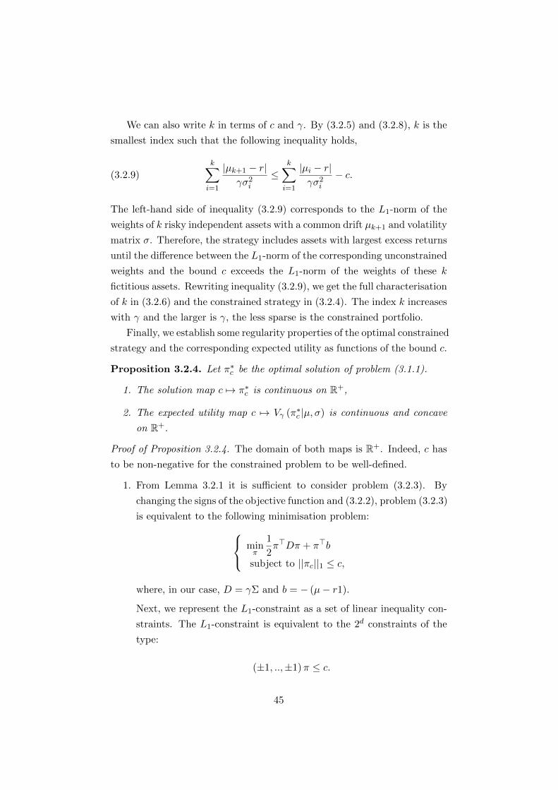
We can also write k in terms of c and γ. By (3.2.5) and (3.2.8), k is the

smallest index such that the following inequality holds,

k∑

i=1

|µk+1 − r|γσ2

i

≤k∑

i=1

|µi − r|γσ2

i

− c.(3.2.9)

The left-hand side of inequality (3.2.9) corresponds to the L1-norm of the

weights of k risky independent assets with a common drift µk+1 and volatility

matrix σ. Therefore, the strategy includes assets with largest excess returns

until the difference between the L1-norm of the corresponding unconstrained

weights and the bound c exceeds the L1-norm of the weights of these k

fictitious assets. Rewriting inequality (3.2.9), we get the full characterisation

of k in (3.2.6) and the constrained strategy in (3.2.4). The index k increases

with γ and the larger is γ, the less sparse is the constrained portfolio.

Finally, we establish some regularity properties of the optimal constrained

strategy and the corresponding expected utility as functions of the bound c.

Proposition 3.2.4. Let π∗c be the optimal solution of problem (3.1.1).

1. The solution map c 7→ π∗c is continuous on R+,

2. The expected utility map c 7→ Vγ (π∗c |µ, σ) is continuous and concave

on R+.

Proof of Proposition 3.2.4. The domain of both maps is R+. Indeed, c has

to be non-negative for the constrained problem to be well-defined.

1. From Lemma 3.2.1 it is sufficient to consider problem (3.2.3). By

changing the signs of the objective function and (3.2.2), problem (3.2.3)

is equivalent to the following minimisation problem:

minπ

1

2π>Dπ + π>b

subject to ||πc||1 ≤ c,

where, in our case, D = γΣ and b = − (µ− r1).

Next, we represent the L1-constraint as a set of linear inequality con-

straints. The L1-constraint is equivalent to the 2d constraints of the

type:

(±1, ..,±1)π ≤ c.

45

Let 1 = (1, . . . , 1)> the 2d-dimensional vector of ones. In matrix form,

we have

Aπ ≤ c1,

where A = (Aij) with Aij ∈ 1,−1, i = 1, . . . , 2d, j = 1, . . . , d,

and each possible combination of signs appears only once as a row of

A. Therefore, the constrained OLS problem is equivalent to standard

quadratic programming problem:

minπ

1

2π>Dπ + π>b,

subject to Aπ ≤ c1.

Since the matrix D is positive definite, the solution map c 7→ π∗c is

continuous, by Lee et al. (2006, Corollary 3.1).

2. Let v (x) = Kγ exp ((1− γ)Tx), x ∈ R. The function v and the mean-

variance term function Mγ are both continuous on R and Rd, respec-

tively. Since the map c 7→ π∗c is continuous, the map c 7→ Vγ (π∗c |µ, σ)

is continuous as a composition of continuous functions:

c 7→ π∗c 7→Mγ (π∗c ) 7→ v (Mγ (π∗c )) = Vγ (π∗c |µ, σ) .

Note that since π∗c is deterministic the last equality holds.

To show the concavity of the expected utility as a function of c, we

define the functions

f (π) = ||√γσ>π − 1√γσ−1 (µ− r1) ||2, and G (π) = ||π||1.

Both functions are convex on Rd. This implies by Luenberger (1969,

Proposition 1, Section 8.3) that the function w (c) = f (π∗c ) is convex

in c. Moreover, by (3.2.2), Mγ (π∗c ) = −12w (c) + K and the map

c 7→Mγ (π∗c ) is concave in c. Finally, as γ > 1 andKγ < 0, the function

v is concave and increasing. Hence, the expected utility map c 7→Vγ (π∗c |µ, σ) is concave in c as a composition of a concave and increasing

function with a concave function, Vγ (π∗c |µ, σ) = v (Mγ (π∗c )).

46

This result holds for any volatility matrix, and it shows that we can

adjust continuously the sparsity of our strategy while keeping the continuity

and the concavity of the expected utility as a function of c. In particular,

as we relax the constraint, the expected utility of the constrained problem

converges to the expected utility of the Merton ratio; see Corollary B.0.4.

3.3 The Constrained Plug-in Strategy: Sparsity

and Estimation

We first characterise the expected utility for any time-constant L1-constrained

strategy πc independent of W (T ). Similarly to Lemma 2.3.1, the expected

utility is given by the moment generating function of the mean-variance

term Mγ (πc).

Lemma 3.3.1. Assume that πc is a time-constant and possibly random

strategy independent of W (T ) such that ||πc||1 ≤ c. Then,

Vγ (πc|µ, σ) = KγE [exp ((1− γ)TMγ (πc))] .(3.3.1)

The lemma is proved in Appendix B.

For the unconstrained estimated strategy, the expected utility can de-

generate to −∞ for γ ≥ 1, as the number of available risky assets increases.

The first advantage of using an L1-norm is to rule out the degeneracy of the

expected utility as the number of assets grows to infinity.

Proposition 3.3.2. Assume that π(d)c is a time-constant and possibly ran-

dom strategy independent of W (d)(T ) such that ||π(d)c ||1 ≤ c for each d.

Suppose

limd→∞

maxi=1,..,d

|µ(d)i − r| <∞ and lim

d→∞max

i,j=1,..,dΣ

(d)ij <∞,

then Vγ

(π

(d)c |µ(d), σ(d)

)is bounded from below for γ ≥ 1 as d→∞.

The statement is proved in Appendix B.

Note that this statement is true for any type of constant L1-constrained

strategy. Hence, this does include plug-in strategies in which drift and pos-

sibly even covariances are replaced by estimators.

47

We see that the L1-constraint is especially helpful when we face pa-

rameter uncertainty for a large number of assets. Indeed, the loss due to

estimation accumulates and it is so large that we can potentially gain from

holding a sparse portfolio. The key to the performance of the L1-constraint

is the trade-off between the gain due to diversification and the loss due to

estimation error.

To understand this in terms of loss functions, let π∗ be the Merton

strategy and π∗c the solution of the constrained problem with the true drift

µ and bound c. When µ is known, the sparsity of the constrained strategy,

π∗c , implies a loss in expected utility. We define the loss factor Lγ (π∗c , π∗)

by the relationship

Vγ (π∗c |µ, σ) = Lγ (π∗c , π∗)Vγ (π∗|µ, σ) .

At the beginning of the investment period, the value of the MLE of

the drift µ is fixed and we obtain the constrained plug-in strategy πc by

solving (3.2.3) with µ and the bound c. The resulting strategy πc is not

normally distributed and it is a biased estimator of π∗c . Thus, there is loss

due to estimation on the constrained strategy. The corresponding loss factor

Lγ (πc, π∗c ) is defined by

Vγ (πc|µ, σ) = Lγ (πc, π∗c )Vγ (π∗c |µ, σ) .

The total loss consists of both the loss due to insufficient diversification

and the loss due to estimation error, i.e., the total loss factor Lγ (πc, π∗) is

defined by

Lγ (πc, π∗) = Lγ (π∗c , π

∗)Lγ (πc, π∗c )

and then we obtain

Vγ (πc|µ, σ) = Lγ (πc, π∗)Vγ (π∗|µ, σ) .

By Proposition 3.2.4, the loss factor due to under-diversification is con-

tinuous in c. The loss factor due to estimation and the total loss factor are

also continuous functions in the bound c as the following proposition shows.

48

Proposition 3.3.3. Let tobs be large enough such that

tobsγΣ + (1− γ)Td||Σ||∞Id

is positive definite. Then, the maps

c 7→ Lγ (πc, π∗c ) and c 7→ Lγ (πc, π

∗)

are continuous on R+.

Proof Proposition 3.3.3. By (2.3.1), the maximum likelihood of the drift,

µ is a Rd-valued random variable on the probability space (Ω,F ,P). To

compute the plug-in constrained strategy, we solve problem (3.2.3) with

µ. In Proposition 3.2.4, we showed that for a fixed value of the drift the

solution map is continuous. Hence, the solution map of the plug-in strategy

(ω, c) 7→ πc is F-measurable and continuous in c a.s..

As in Proposition 3.2.4, let v (x) = Kγ exp ((1− γ)Tx), with Kγ < 0.

Our objective is to show that |v (Mγ (πc)) | ∈ L1 (Ω,F ,P). Indeed, since the

map c 7→ v (Mγ (πc)) is continuous, we can then establish the continuity of

the map c 7→ E (v (Mγ (πc))) = Vγ (πc|µ, σ) by the dominated convergence

theorem.

We start by computing a lower bound for the mean-variance termMγ (πc)

(inequalities hold a.s.):

Mγ (πc) = π>c (µ− r1)− γ

2π>c Σπc ≥ −||πc||1||µ− r1||∞ −

γ

2||Σ||∞||πc||21.

Since ||πc||1 ≤ ||π||1, we deduce that

Mγ (πc) ≥ −||π||1||µ− r1||∞ −γ

2||Σ||∞||π||21,

and we define

Y = −||π||1||µ− r1||∞ −γ

2||Σ||∞||π||21.(3.3.2)

Because the function v is increasing and negative, v (Y ) ≤ v (Mγ (πc)) and

|v (Mγ (πc)) | ≤ |v (Y ) |.To apply the dominated convergence theorem, we need to show that

49

|v (Y ) | ∈ L1 (Ω,F ,P). Note that

E (|v (Y ) |) = −KγE[exp

((γ − 1)T

(||π||1||µ− r1||∞ +

γ

2||Σ||∞||π||21

))]

and by Cauchy-Schwarz inequality in L2 (Ω,F ,P) we obtain

(E[|v (Y ) |])2 ≤ K2γE [exp (2 (γ − 1)T ||π||1||µ− r1||∞)](3.3.3)

· E[exp

((γ − 1) γT ||Σ||∞||π||21

)].(3.3.4)

Therefore, we have to show that the two expectations on the right hand side

of the inequality are finite. Recall that π ∼ Nd(π∗, V 2

0

). We set V 2

0 = V V >

with V ∈ Rd×d. Let z ∼ N (0, 1), Z ∼ Nd (0, Id),

a = 2 (γ − 1)T ||µ− r1||∞||V ||∞ and C = exp (2 (γ − 1)T ||µ− r1||∞||π∗||1) .

For γ > 1 the first expectation in (3.3.3) can be bounded as follows,

E [exp (2 (γ − 1)T ||π||1||µ− r1||∞)]

= E[exp

(2 (γ − 1)T ||V Z + π∗||1||µ− r1||∞

)],

≤ CE[exp

(2 (γ − 1)T ||µ− r1||∞||V ||∞||Z||1

)],

= C(E[exp

(2 (γ − 1)T ||µ− r1||∞||V ||∞|z|

)])d,

= C

(2 exp

(a2

2

)Φz (a)

)d, where Φz the CDF of z,

<∞.

Since ||π||21 ≤ d||π||22, the second expectation in (3.3.3) can be bounded

as follows:

E[exp

((γ − 1) γT ||Σ||∞||π||21

)]≤ E

[exp

((γ − 1) γTd||Σ||∞||π||22

)],

which is finite by Lemma A.0.3 because(V 2

0

)−1 − (γ − 1) γTd||Σ||∞Id is

positive definite as(V 2

0

)−1= γ2tobsΣ. This condition is equivalent to

tobsγΣ + (1− γ)Td||Σ||∞||Id being positive definite.

The proof consists in showing that the map c 7→ Vγ (πc|µ, σ) is con-

tinuous. Because the term (1− γ)Td||Σ||∞ is negative and grows linearly

50

with d, Proposition 3.3.3 can be applied only if tobs is roughly larger than

d. If the L1-constraint effectively shrinks all the weights towards zero, i.e.,

| (πc)i | ≤ |πi|, for i = 1, . . . , d, a.s., we can get rid of the dependency on

d. In this case, the continuity holds if tobsγΣ + (1− γ)T ||Σ||2Id is positive

definite. This property is in particular true for a diagonal covariance matrix.

Remark 3.3.4. If ||πc||2 ≤ ||π||2 a.s., then

π>c Σπc ≤ λmax (Σ) ||πc||22 ≤ λmax (Σ) ||π||22 a.s.,

with λmax (Σ) = max||Σx||2 : x ∈ Rd with ||x||2 = 1

. Therefore, we can

set the lower bound in (3.3.2) as

Y = −||π||1||µ− r1||∞ −γ

2λmax (Σ) ||π||22.

Then, |v (Y ) | ∈ L1 (Ω,F ,P) if tobsγΣ + (1− γ)Tλmax (Σ) Id is positive def-

inite.

As we relax the constraint, the strategy π∗c is more diversified and the

term Lγ (π∗c , π∗) converges to one, i.e.,

Lγ (π∗c , π∗)→ 1 as c→∞.(3.3.5)

The loss factor due to estimation error, Lγ (πc, π∗c ), behaves oppositely. As c

increases, more stocks are included in the strategy and the estimation error

forces Lγ (π∗c , πc) to move away from one. By Proposition 3.3.3, the loss

factor Lγ (πc, π∗c ) and the total loss factor Lγ (πc, π

∗) both converge to the

loss factor of the unconstrained plug-in strategy6, i.e.,

Lγ (πc, π∗c )→ Lγ (π, π∗) and Lγ (πc, π

∗)→ Lγ (π, π∗) as c→∞.(3.3.6)

For tobs and c finite, the loss factors are bigger than one and the aim is to

find a bound such that the total loss factor is closest to one. The existence

of an optimal bound depends on the structure of the true parameters and

the accuracy of the estimator µ. We study the behaviour of the loss factors

in more detail in the next section.

Remark 3.3.5. As in the unconstrained case, the measure of efficiency, in-

troduced in Definition 2.3.5, is a function of the loss factor of the constrained

6See Corollary B.0.4 in the Appendix.

51

plug-in strategy. Since the expected utility is given by (3.3.1), the following

relationship holds true for γ > 1:

Θγ (πc) = Lγ (πc, π∗)

11−γ .

3.4 Simulation Study

In this section, we investigate the structure and the performance of the

L1-constrained portfolio when risky assets are correlated. We consider a

volatility matrix that is non-diagonal. For this situation we do not have an

analytic form for the constrained strategy and therefore we use simulations

to compute its expected utility. Our data set consists of a random sample of

d = 250 stocks that have been listed at least once on the S&P 500 and had

daily returns for all trading days between January 2001 and December 2011.

There is no problem of survivorship bias because our main goal is to show the

existence and the uniqueness of an optimal bound c for a given universe of

stocks. Throughout this section, we assume an initial normalised endowment

of X (0) = 1, an annual risk-free rate of r = 0.02 and an investment horizon

of T = 1 year.

3.4.1 Methodology

Based on the daily log-returns of the stocks, we compute the following un-

biased estimators µ, Σ of µ and Σ respectively:

µ =1

∆ξ +

1

2diag

(Σ),(3.4.1)

Σij =1

∆ (N − 1)

N−1∑

k=0

[Ri (k)− ξi

] [Rj (k)− ξj

], for i, j = 1, . . . , d,

(3.4.2)

with ξi =1

N

N−1∑

k=0

Ri (k) and Ri (k) = log(Si((k+1)∆)Si(k∆)

). The time step is

defined by ∆ = tobs/N , with tobs = 11 years and N = 2767 days.

We then assume a standard Merton market as introduced in Section 2.2

where we set µ = µ for the drift and Σ = Σ for the covariance matrix.

Furthermore, we evaluate the estimator of the drift µ by sampling from its

52

law, i.e., we use the fact that µ ∼ Nd (µ,Σ/tobs). In this setting, we compute

the investment weights and the associated expected utility for :

• π∗ the unconstrained strategy using the true µ,

• π the unconstrained plug-in strategy using the estimator µ,

• π∗c the L1-constrained strategy using the true µ,

• and π∗c the L1-constrained plug-in strategy using the estimator µ.

For a non-diagonal volatility matrix, we do not have analytical results

for the L1-constrained strategy. Therefore, we compute the optimal weights

numerically. To do so, we plug the true or the estimated drift in (3.2.1) and

we solve the quadratic optimisation problem with the LARS algorithm; see

Efron et al. (2004). This algorithm generates the optimal portfolio weights

for all binding bounds.

3.4.2 Computation of the Loss Function

We want to compute the expected utility of the unconstrained and the con-

strained strategies both when the drift is known and when it is estimated.

For the unconstrained case, we know the explicit form of the expected util-

ity associated with the Merton ratio (2.2.3) and the plug-in strategy (2.3.2).

For the constrained case with known drift, the strategy is deterministic and

the associated expected utility can be computed directly by using (3.3.1).

When the drift is estimated, the constrained strategy πc is random, and

we approximate its expected utility using a Monte-Carlo method. More

specifically, we sample M i.i.d. realisations of the MLE of the drift. Then,

for each realisation, we solve for the associated constrained strategy and we

obtain i.i.d. realisations Y 1γ,c, . . . , Y

Mγ,c of Yγ,c given by

Yγ,c = exp(

(1− γ)T(π>c (µ− r1)− γ

2π>c Σπc

)).

For Kγ given in (2.2.4), we define the Monte-Carlo estimator of the expected

utility by

Vγ,M (πc|µ, σ) = Kγ1

M

M∑

i=1

Y iγ,c,

53

which approximates Vγ (πc|µ, σ) = KγE (Yγ,c); see (3.3.1). The accuracy

of the method is measured by the standard deviation of the Monte-Carlo

estimator given by

√Var

(Vγ,M (πc|µ, σ)

).

For a fixed c, the standard deviation of the random variable Vγ,M (πc|µ, σ)

is a function of γ. Therefore, the number of realisations necessary to attain

a given accuracy varies with γ. In this section, the number of realisations,

M , is fixed to 5000 for all γ ∈ [1, 7]7.

Furthermore, the loss in expected utility due to estimation Lγ (πc, π∗c )

is approximated by the ratio of the Monte-Carlo estimator Vγ,M (πc|µ, σ)

and the expected utility of the constrained strategy with known parameters

Vγ (π∗c |µ, σ). To remove the influence of the multiplicative factor Vγ (π∗c |µ, σ)

on the accuracy of the estimation of the loss factors, we apply the logarithmic

transformations:

`γ (π∗c , π∗) = log (Lγ (π∗c , π

∗)) , `γ (πc, π∗c ) = log (Lγ (πc, π

∗c )) .

As mentioned in Section 3.3, the total loss in expected utility is the prod-

uct of the loss due to under-diversfication measured in terms of the factor

Lγ (π∗c , π∗), and the loss due to estimation, measured in terms of the factor

Lγ (πc, π∗c ). The logarithm of the total loss factor is then given by

`γ (πc, π∗) = `γ (π∗c , π

∗) + `γ (πc, π∗c ) .

Computing the logarithm enables us to have a natural interpretation of the

loss factors. Indeed, in this additive setting, the log-loss equals to zero

when there is no loss in expected utility. By (3.3.5) and (3.3.6), the log-

loss factors converge to zero and to the log-loss factor of the unconstrained

plug-in strategy, respectively,

`γ (π∗c , π∗)→ 0, `γ (πc, π

∗c )→ `γ (π, π∗) , and `γ (πc, π

∗) ,→ `γ (π, π∗) .

as c → ∞. Finally, as the log-convexity implies the convexity of the loss

function itself, it is sufficient to study the convexity of the log-loss.

7See discussion in Appendix C.

54

3.4.3 Existence of an Optimal Bound

Figure 3.1 depicts the profile of the log-loss factor as a function of c for γ = 5.

We see that the log-loss factors are continuous in c. Furthermore, the total

log-loss, `γ (πc, π∗), is convex in c and it is minimised at c∗ = 12. Hence, the

total loss factor Lγ (πc, π∗) is also convex and minimised at c∗. Equivalently,

the expected utility of the constrained plug-in strategy is maximised at this

optimal bound c∗.

0

1

2

3

4

5

6

7

5 10 15 20 25 30 35 40

log(

Loss

)

L1-constraint (c)

Under-diversificationEstimation

Total

Figure 3.1: Plot of the log-loss factor due to under-diversification `γ (π∗c , π∗),

due to estimation `γ (πc, π∗c ) and the total loss factor `γ (πc, π

∗) as a functionof the bound of the L1-constraint c with γ = 5.

RRA Optimal L1-constrained Unconstrainedγ c `γ (πc, π

∗) Θγ (πc) `γ (π, π∗) Θγ (π)

2 29 2.88 0.06 5.82 0.0033 20 3.86 0.15 7.82 0.025 12 4.63 0.31 9.44 0.107 8 4.97 0.44 10.14 0.19

Table 3.1: Comparison of the log-loss in expected utility and the efficiencybetween the constrained and the unconstrained case, for different values ofrisk aversion γ. The log-loss factor is equal to zero when there is no loss.

Table 3.1 shows that the optimal bound decreases sharply with γ. Again,

as γ increases, we need to use a more restrictive bound to optimally control

the loss factor. For each γ, the loss due to underdiversification represents

between 41% and 44% of the total loss factor, while loss due to estimation

55

represents between 56% and 59%. Moreover, the L1-constraint greatly helps

the log-loss to be closer to zero. The logarithm of the loss is reduced by

roughly 50% at the optimal bound and the loss factor itself is reduced by at

least 95.7%.

In terms of efficiency, the L1-constraint also helps significantly. For small

levels of risk aversion, e.g., γ = 2, 3, the efficiency is improved dramatically

by imposing an L1-constraint. For high level of risk aversion, e.g., γ = 7,

the effect of estimation is less important, as a smaller fraction is invested

in the risky assets. In this case, holding a L1-sparse portfolio doubles the

efficiency of the investor.

3.4.4 Structure and Stability of the L1-constrained Strategy

Regarding the sparsity of the constrained strategy, the results of Section 3.2

extend to our general covariance matrix. Figure 3.2 shows that the number

of stocks invested in increases with γ. For instance, at c = 7, we invest in

44 stocks with γ = 2 and in 93 stocks with γ = 6.

On the one hand, if γ is large, we are less constrained as a smaller

fraction is invested in each selected stock, and this enables us to hold a

more diversified portfolio. On the other hand, if γ is small, we still take

some relatively strong positions at the cost of having a very sparse portfolio.

As we relax the constraint, we notice that the number of stocks invested

in increases stepwise. The steps are especially long for small γ as we take

large positions. In effect, c needs to be increased significantly until new

stocks are added to the portfolio.

For independent stocks, we should invest in stocks with the highest abso-

lute excess returns up to a certain index k, which is increasing in γ (Theorem

3.2.2). The weights of the selected stocks are shrunk towards zero, while the

other weights are set to zero. If stocks with highest absolute returns have

positive excess returns, the portfolio consists exclusively of long positions

and the L1-constraint acts only as a restriction of the number of stocks.

Table 3.2 reports the composition on the L1-constrained portfolio for

correlated stocks, when the drift µ is known. Because of the structure of the

covariance matrix, stocks with negative returns are selected although their

absolute excess return is close to zero. Indeed, the L1-constraint selects

the stocks with highest returns and then jumps to stocks with negative

excess returns. In contrast to the no-short sale constraint, we still keep a

56

0

50

100

150

200

250

0 2 4 6 8 10 12 14 16 18 20

# of

Sto

cks

L1-constraint(c)

γ = 1γ = 2γ = 4γ = 6γ = 8

Figure 3.2: Number of stocks invested in as a function of the bound c of theL1-constraint for different RRA coefficients γ. We have chosen r = 0.02 forthe annual risk-free rate.

limited proportion of short positions. The short positions represent 47% of

the amount of the L1-norm of the unconstrained portfolio while they are

reduced to 30 % for the constrained case when we use L1-bound c = 3.

Hence, the constraint controls both the sparsity and the proportion of short

positions; see also Remark 3.1.3.

In Table 3.3, we compare the structure of the plug-in strategies, when

the drift is estimated using (3.4.1) and γ = 2. For the L1-constrained

strategy, the bound c is chosen to be the optimal bound minimising the

loss in expected utility, as in Table 3.1. We report the expected value of

the number of stocks invested in, the number of shorts positions, and the

fraction in L1-norm of short positions. At the optimal bound, the number

of stocks and short positions is reduced from 250 to approximately 86 stocks

and from approximately 121 to 41 positions, respectively.

For the unconstrained strategy, the number and the fraction in L1-norm

of short positions both represent 48.36% of the positions and the L1-norm

respectively. We demonstrated in Table 3.2 that, by taking a restrictive

bound, the proportion of short positions is reduced substantially. At the

optimal bound, this is not the case. Indeed, the number of short positions

57

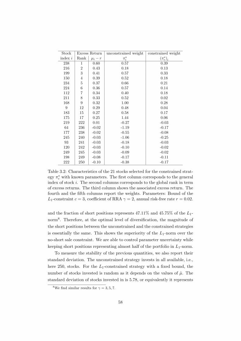
Stock Excess Return unconstrained weight constrained weightindex i Rank µi − r π∗i (π∗c )i

238 1 0.60 0.57 0.39216 2 0.43 0.18 0.13199 3 0.41 0.57 0.33150 4 0.39 0.52 0.18234 5 0.37 0.66 0.21224 6 0.36 0.57 0.14112 7 0.34 0.40 0.18211 8 0.33 0.52 0.02168 9 0.32 1.00 0.289 12 0.29 0.48 0.04

183 15 0.27 0.58 0.17175 17 0.25 1.44 0.06219 222 0.01 -0.27 -0.0364 236 -0.02 -1.19 -0.17177 238 -0.02 -0.55 -0.08245 240 -0.03 -1.06 -0.2593 241 -0.03 -0.18 -0.03120 242 -0.03 -0.10 -0.02249 245 -0.03 -0.09 -0.02198 249 -0.08 -0.17 -0.11222 250 -0.10 -0.38 -0.17

Table 3.2: Characteristics of the 21 stocks selected for the constrained strat-egy π∗c with known parameters. The first column corresponds to the generalindex of stock i. The second columns corresponds to the global rank in termof excess returns. The third column shows the associated excess return. Thefourth and the fifth columns report the weights. Parameters: Bound of theL1-constraint c = 3, coefficient of RRA γ = 2, annual risk-free rate r = 0.02.

and the fraction of short positions represents 47.11% and 45.75% of the L1-

norm8. Therefore, at the optimal level of diversification, the magnitude of

the short positions between the unconstrained and the constrained strategies

is essentially the same. This shows the superiority of the L1-norm over the

no-short sale constraint. We are able to control parameter uncertainty while

keeping short positions representing almost half of the portfolio in L1-norm.

To measure the stability of the previous quantities, we also report their

standard deviation. The unconstrained strategy invests in all available, i.e.,

here 250, stocks. For the L1-constrained strategy with a fixed bound, the

number of stocks invested is random as it depends on the values of µ. The

standard deviation of stocks invested in is 5.78, or equivalently it represents

8We find similar results for γ = 3, 5, 7.

58

Expected value of Weightsγ = 2 #i : (πc)i 6= 0 #i : (πc)i < 0 ||π−c ||1/|||πc||1 (%) std. dev.

Merton 250 (0.00) 120.92 (4.81) 48.36 (0.47) 0.66L1, c = 29 86.39(5.78) 40.70 (4.27) 45.75 (1.71) 0.21

Table 3.3: This table reports the expected value (and standard deviation) ofthe number of stocks invested in, the number of shorts positions, the fractionin L1-norm of short positions and the average of the standard deviation ofthe weights. The quantities presented are the sample mean and standarddeviation over M = 5000 realisations. The optimal bound c of the L1-constrained strategy is chosen as in Table 3.1. The unconstrained Mertonplug-in strategy corresponds to c = ∞. Parameters: Coefficient of RRAγ = 2, annual risk-free rate r = 0.02.

6.7% of the expected number of stocks held in the portfolio. Compared to

the unconstrained strategy, the variability of the number and the fraction in

L1-norm of short positions is proportionally higher for the L1-constrained

strategy. While the structure of the portfolio is more sensitive to the esti-

mation of the drift, the overall stability of the portfolio is improved. Indeed,

the average standard deviation of the weights is 68.2% smaller for the con-

strained strategy. Since the L1-norm of the weights is bounded, extreme

positions are forbidden and in turn variability is reduced.

59

Chapter 4

Out-of-Sample Study

Our goal is to investigate the out-of-sample structure and performance of

the unconstrained and the optimally constrained plug-in strategies using

empirical data. Therefore we will no longer have any parametric assumptions

on the evolution of the asset prices.

From the theoretical considerations in the previous chapters, we have

learned the following: We should rebalance our portfolio as frequently as

possible (i.e., continuously in the best case). We will therefore trade daily

on daily data. To reduce the effect of parameter uncertainty, we should

choose a suitable bound c for the L1-constraint. This is what we do by

selecting the bound maximising the utility as we will discuss in detail in

Section 4.1. Finally, we measure the performance of the strategies in terms

of (expected) utility of terminal wealth.

When looking at the out-of-sample results, we need to keep in mind

that the performance of the strategies is now also affected by the effects

of discrete trading and discrete observations which was not the case in the

previous sections. This is a problem that arises with all continuous-time

models.

Our data set consists of the stocks that have been listed at least once

in the S&P 500 and had daily returns for all trading days between January

2001 and December 2011.

We test our method between 2006 and 2011. At the beginning of each

year, we select randomly a sample of 250 stocks and we fix it as the universe

of stocks to invest in. Based on the five previous years of daily returns, we

estimate the drift and volatility matrix of these stocks. We calibrate the

60

optimal bound of the L1-constraint as outlined in Section 4.1.

Trading now takes place over intervals of a length of one month. At the

beginning of each month, we assume a normalised initial endowment of one

unit of cash and an annual risk-free rate of r = 0.02. At the end of the

month we record the terminal utility. We average the terminal utilities that

we obtain from trading 24 times consecutively over a one month interval,

i.e., a two years period. We consider three consecutive time periods of two-

years length and compare the performance of the plug-in strategies to the

equally-weighted portfolio, which is a hard benchmark to beat; see DeMiguel

et al. (2009b).

4.1 Choosing the L1-bound

To find a suitable (and ideally optimal) bound for the L1-constraint c, we

present two alternative methods, namely a method that we call the leave-

one-block-out method (LOB) and a cross-validation method (CV).

For both methods we start as follows. On the first trading day of each

month, we divide the multivariate time series of daily returns of the five

previous years into 60 blocks of one month. Based on the 59 first blocks,

we estimate the drift and the volatility matrix using (3.4.1) and (3.4.2).

Next, we compute the constrained plug-in strategy in the interval [0, ||π||1]

for each value of the bound c that is on a grid with grid size ∆c = 0.1.

Finally, we invest (rebalancing daily) on the remaining block with respect

to the constrained plug-in strategy; see also (4.2.1).

In the leave-one-block-out (LOB) method, we select the bound c max-

imising the utility of final wealth. In the cross-validation (CV) method, we

repeat this procedure 1000 times by taking a random sample with replace-

ment of the 60 blocks and we select the bound c maximising the average

utility of final wealths.

As the method of estimation is the same for all months, estimation risk

is constant through time and the variation of the optimal bound depends

mainly on the market conditions of the calibration period.

Table 4.1 contains the numerical results for the optimal L1-bounds using

the two different methods. For the LOB method, the optimal bound varies

widely. While the first quartile stays small over all periods, the median

(mean) and the third quartile are of different magnitude within and across

61

each period. Moreover, there are five months in 2008, and three months

in 2009, with an optimal bound equal to zero. During these months, the

strategy consists in holding only the risk-free asset.

In 2006-2007 and 2010-2011, the evolution of the optimal bound cal-

ibrated with the CV method is stable as the difference between the first

quartile and the third quartile is small. In 2008-2009, there is a large vari-

ation of the optimal bound because it is a period of transition. Indeed, the

mean over time of the optimal bound is 20.62 in 2008 and 5.03 in 2009.

Furthermore, we observe a substantial drop in the median (mean) of the

optimal bound, from 12.00 (13.39) in 2006-2007 to 3.25 (3.27) in 2010-2011.

In 2010-2011, the CV method incorporates the fact that preceding years

were very volatile and it delivers a more conservative and restrictive bound.

Optimal L1-Bound1st Quartile Median (Mean) 3rd Quartile

2006-2007LOB 0.78 21.65 (65.00) 68.42CV 10.85 12.00 (13.39) 15.02

2008-2009LOB 0.00 1.80 (29.78) 23.20CV 3.93 10.90 (12.82) 20.32

2010-2011LOB 0.65 5.10 (44.63) 91.15CV 2.20 3.25 (3.27) 4.60

Table 4.1: This table reports the summary statistics of the optimal boundsc for the leave-one-block out (LOB) and the cross validation (CV) methodsfor the three time periods that we consider. Parameters: Coefficient of RRAγ = 2, investment horizon T = 1/12, and annual risk-free rate r = 0.02

4.2 Performance of the Plug-in Strategies

At the beginning of each month we pick the optimal L1-bound which was

identified with one of our two methods. We estimate the drift and the

volatility matrix using (3.4.1) and (3.4.2) based on the past five years of

daily returns. Then we compute the unconstrained and the constrained

plug-in strategies. The strategies are then held constant over a period of

one month, i.e., T = 1/12. This means we rebalance the positions daily to

62

keep the weights constant over the investment period. For each month M

and strategy πM which is constant in time over the month, the dynamics of

the wealth denoted by XM is given by

XM (t+ 1) = XM (t)

(1 + rd +

d∑

i=1

πMi (ri(t+ 1)− rd)),(4.2.1)

where rd is daily risk-free rate and ri(t+ 1) is the simple net return of asset

i between day t and day t+1. Since there are 21 trading days in one month,

we have t = 0, . . . , 20. At the end of each month M , we obtain a utility of

final wealth Uγ(XM (20)

).

In Table 4.2, we report the summary statistics of the utility of final

wealth for three blocks of two years, i.e., M = 1, . . . , 24 in each block. Over

all periods, the unconstrained plug-in strategy performs poorly, because

of its extreme variance. For instance, the unconstrained strategy gives its

highest return in August 2007, and directly leads to bankruptcy a month

later. Furthermore, the standard deviation of monthly returns of the wealth

is at its peak in 2006-2007 with a magnitude of 1219.95%. Although on a

smaller scaler, its remains between 89.61% and 120.02% over the subsequent

periods. As a result, from January 2008 to May 2009, the wealth reaches zero

in almost every month. As we measure the performance with a power utility

function with γ > 1, hitting zero for the wealth translates into infinitely

negative utility.

The constrained plug-in strategy calibrated with a bound with the LOB

method is halfway between the unconstrained strategy and the constrained

strategy calibrated with the CV method. It is the most successful strategy

for two periods, with a utility of -0.74 in 2006-2007 and of -0.81 in 2010-

2010. This performance comes at the cost of a very large variance of monthly

returns. In terms of standard deviation of utility of final wealth and monthly

returns, the strategy is similar to the unconstrained portfolio. Therefore,

amidst the financial crisis of 2008-2009, the wealth also hits zero.

The constrained plug-in strategy calibrated with the CV method per-

forms better than the unconstrained strategy in all periods and it is more

stable over time than both the unconstrained and the L1-constrained with

LOB strategies. Although, on average, its returns have a larger standard de-

viation than the equally-weighted portfolio, the mean utility of final wealth

63

is comparable in all periods. The utility of the constrained strategy is higher

in 2006-2007, measuring -0.97 versus -0.99. In 2008-2009, the large propor-

tion of estimated short positions hurts the performance of the constrained

strategy and it has a smaller mean utility of -1.46 versus -1.01. Finally the

mean utility of final wealth is equal for both strategies in 2010-2011 with a

value of -0.99.

Given the nature of the out-of-sample study trading takes place in dis-

crete time. It is well-known that strategies that are optimal in continuous-

time cannot just be discretised to obtain strategies that are optimal in

discrete-time; see Rogers (2001) and Bauerle et al. (2013) for extensive dis-

cussion. In particular, short-selling is never optimal when trading takes

place in discrete-time. Since in our study the L1-constraint does not rule

out short-selling, the superiority of the L1-constrained portfolio over the

unconstrained portfolio is not just a consequence of no short-selling.

Utility of Final Wealth Return of Portfolio (%)

Min. Mean (std.dev.) Max Min. Mean (std.dev.) Max.

2006-2007

Merton −∞ −∞ -0.02 -100 290.84 (1219.95) 5765.79L1, c with LOB -1.00 -0.74 (0.32) -0.02 0.17 355.86 (1201.51) 5765.79L1, c with CV -1.38 -0.97 (0.26) -0.43 -27.36 12.88 (41.37) 134.02EWE -1.08 -0.99 (0.03) -0.95 -7.44 1.01 (3.14) 5.09

2008-2009

Merton −∞ −∞ -0.29 -100 -60.07 (89.61) 245.44L1, c with LOB −∞ −∞ -0.12 -100 66.57 (170.09) 744.64L1, c with CV -4.95 -1.46 (0.99) -0.29 -79.81 0.55 (72.24) 242.19EWE -1.27 -1.01 (0.13) -0.74 -21.35 0.59 (12.95) 34.50

2010-2011

Merton -10.11 -2.43 (2.55) -0.20 -90.11 6.39 (120.02) 398.11L1, c with LOB -1.00 -0.81 (0.24) -0.20 0.17 48.25 (99.01) 398.11L1, c with CV -1.17 -0.99 (0.08) -0.86 -14.28 1.48 (8.22) 15.72EWE -1.13 -0.99 (0.06) -0.87 -11.56 1.07 (6.19) 15.21

Table 4.2: This table reports the summary statistics of the utility and themonthly returns of final wealth out-of-sample. The quantities presented arecomputed over each block of 24 months. The optimal bounds c of the L1-constrained strategies are calibrated using the leave-one-block-out (LOB)and the cross-validation (CV) methods. Parameters: Coefficient of RRAγ = 2, initial wealth XM (0) = 1, investment horizon T = 1/12, and annualrisk-free rate r = 0.02.

64

4.3 Structure and Stability of the Strategies

In Table 4.3, we report the mean and standard deviation of stocks invested

in, of the short positions, of the fraction of short positions in L1-norm and

the mean of the monthly portfolio turnover for four differernt investment

strategies: the unconstrained Merton strategy, referred to as Merton in Ta-

ble 4.3, the L1-constrained strategy where the bound was computed using

the LOB-method, the L1-constrained strategy where the bound was com-

puted using the CV-method, and the equally weighted portfolio, referred to

as EW.

The monthly portfolio turnover is defined as

Monthly Turnover =1

20

21∑

t=2

d∑

i=1

(|πi − πi

(t−)|),

where πi is the constant target weight for asset i, and πi (t−) is the fraction

of wealth (i.e., the weight) invested in asset i just before rebalancing at time

t. All portfolios are rebalanced daily and 21 corresponds to the number of

trading days in a month. If the wealth hits zero during the month, we set

the turnover to ∞ and stop the rebalancing.

For the unconstrained strategy, the structure remains unchanged through-

out the whole test period. The mean fraction of short positions of the L1-

norm stays between 120 and 124, the mean ratio ||π−||1/||π||1 stays between

47% and 50% and the portfolio turnover is infinite both in 2006-2007 and

2008-2009. It is finite in 2010-2011, but still large.

For the constrained plug-in strategy with the LOB method, the mean

number of risky assets invested in and that of short positions is the largest

in 2006-2007 and 2010-2011. In 2008-2009, these quantities are significantly

smaller, because there are actually several months where there is no invest-

ment in risky assets; see also Table 4.1. Nevertheless, on average, the mean

ratio ||π−||1/||π||1 stays stable over each period, with a larger standard devi-

ation in 2008-2009. In terms of turnover, the strategy performs poorly. The

turnover is very high in 2006-2007 and it is infinite in 2008-2009. In 2010-

2011, it is reduced but still much larger than the turnover of the constrained

plug-in strategy calibrated with the CV method and the equally-weighted

portfolio. This turnover is high because of the variability of the optimal

bound to different market conditions.

65

For the constrained plug-in strategy calibrated with the CV method,

the mean number of risky assets invested in and that of short positions de-

creases in each period. The mean fraction of short positions of the L1-norm

does not. The mean ratio ||π−||1/||π||1 is actually the largest in 2008-2009,

with a value of 44.74%, and it is similar in 2006-2007 and 2010-2011, with

35.48% and 33.47%, respectively. For 2008-2009, the mean of estimated

excess returns decreases sharply during the year 2008 and it implies a sig-

nificantly larger fraction of short positions in the constrained portfolio.The

constrained plug-in strategy calibrated with the CV method is more stable

than the constrained plug-in strategy calibrated with LOB method. The

standard deviation of each measure is reduced by at least 40%. Finally,

although its turnover is much larger than the equally-weighted portfolio

turnover in 2006-2007 and 2008-2009, the turnovers are comparable during

the period 2010-2011.

4.4 Transaction Costs

For a complete analysis of the out-of-sample performance it is interesting to

consider transaction costs as well. It is well-known that if transaction costs

are included, holding the Merton ratio and hence having to continuously

rebalance the portfolio is no-longer optimal. In particular, the investor can

find herself in a position where it is optimal not to trade at all. This would

happen if her positions would be within the so-called no-trading region which

is used to characterise the optimal trading strategies; see, e.g., Davis and

Norman (1990). Nevertheless, we can still investigate what transaction costs

one would have to pay when using the trading strategies that we have derived

in our setting without transaction costs.

Keim and Madhavan (1998) distinguish implicit costs such as the bid-

ask spread which are proportional to the cash amount of shares traded,

and explicit trading costs, such as brokerage commissions, which are fixed

costs per share traded. They measure both types of trading costs as a

percentage of the face value of investment. However, Goldstein et al. (2009)

argue that brokerage commissions should not be measured as a percentage

of face value. Indeed, brokers ignore most available prices and they charge

commissions in exact cents per share. Moreover, large trades tends to have

higher commissions fees per share and they may also have larger proportional

66

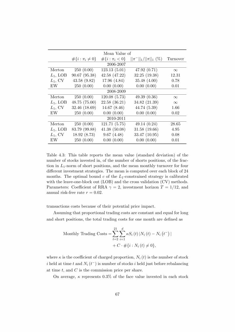
Mean Value of#i : πi 6= 0 #i : πi < 0 ||π−||1/||π||1 (%) Turnover

2006-2007

Merton 250 (0.00) 123.13 (5.01) 47.92 (0.71) ∞L1, LOB 90.67 (95.38) 42.58 (47.22) 32.25 (19.38) 12.31L1, CV 43.58 (9.82) 17.96 (4.84) 35.48 (4.00) 0.78EW 250 (0.00) 0.00 (0.00) 0.00 (0.00) 0.01

2008-2009

Merton 250 (0.00) 120.08 (5.73) 49.39 (0.36) ∞L1, LOB 48.75 (75.00) 22.58 (36.21) 34.82 (21.39) ∞L1, CV 32.46 (18.69) 14.67 (8.46) 44.74 (5.39) 1.66EW 250 (0.00) 0.00 (0.00) 0.00 (0.00) 0.02

2010-2011

Merton 250 (0.00) 121.71 (5.75) 49.14 (0.24) 28.65L1, LOB 83.79 (99.88) 41.38 (50.08) 31.58 (19.66) 4.95L1, CV 18.92 (8.73) 9.67 (4.48) 33.47 (10.95) 0.08EW 250 (0.00) 0.00 (0.00) 0.00 (0.00) 0.01

Table 4.3: This table reports the mean value (standard deviation) of thenumber of stocks invested in, of the number of shorts positions, of the frac-tion in L1-norm of short positions, and the mean monthly turnover for fourdifferent investment strategies. The mean is computed over each block of 24months. The optimal bound c of the L1-constrained strategy is calibratedwith the leave-one-block out (LOB) and the cross validation (CV) methods.Parameters: Coefficient of RRA γ = 2, investment horizon T = 1/12, andannual risk-free rate r = 0.02.

transactions costs because of their potential price impact.

Assuming that proportional trading costs are constant and equal for long

and short positions, the total trading costs for one month are defined as

Monthly Trading Costs =

21∑

t=2

d∑

i=1

κSi (t) |Ni (t)−Ni

(t−)|

+ C ·#i : Ni (t) 6= 0,

where κ is the coefficient of charged proportion, Ni (t) is the number of stock

i held at time t and Ni (t−) is number of stocks i held just before rebalancing

at time t, and C is the commission price per share.

On average, κ represents 0.3% of the face value invested in each stock

67

and fixed costs commissions C vary between 2 and 5 cents per share. For

simplicity, we take κ = 0.3% and C = 0.025. As a benchmark, we consider a

small investor, with a coefficient of RRA γ = 2 and an initial wealth ofXM0 =

25000, so that trades do not have any price impact. Note that total trading

costs are not proportional to the initial wealth invested. Their dependence

on the initial wealth is especially important for the plug-in strategies as the

number of shares varies widely.

During the financial crisis 2008-2009, the volatility of the markets leads

to a large variability of the positions held in the portfolio even for the con-

strained plug-in strategies; see Table 4.3. As a result, the proportional

transaction costs are much higher for these strategies compared to the

equally-weighted portfolio. During the period 2006-2007 and 2010-2011,

the constrained strategies perform on average at least as well as the equally-

weighted portfolio1. While having a significantly higher performance during

these years, the constrained strategy calibrated with the LOB method faces

large transaction costs. For instance, the average of total trading costs are

6625.08 and 9963.01 units of cash in 2006 and 2010 respectively. In the same

years, the total transaction costs of the constrained strategy calibrated with

CV and the equally-weighted portfolio are 664.34 and 140.35 in 2006, and

95.42 and 140.68 in 2010. Hence, in 2010, both strategies deliver the same

average utility and the transaction costs are on average smaller for the con-

strained strategy.

In summary, outside the financial crisis L1-constrained strategies de-

liver on average a higher utility than the equally-weighted portfolio. Re-

garding transaction costs, the constrained strategies have large proportional

costs and low fixed commissions. Furthermore, because of fixed commissions

the equally-weighted portfolio and the unconstrained portfolio suffer from

complete diversification. The trade-off between the two types of costs de-

pends on the size of the positions and the sparsity of the strategies. For the

constrained strategy with LOB, total trading costs remain large, while the

constrained strategy with CV can have lower trading costs than the equally-

weighted portfolio. Note that the effect of proportional trading costs will be

reduced for a higher level of risk aversion, as the weights in the risky assets,

and in turn the number of shares, decreases with γ.

1In Table 4.2, the utilities are given for an investor with a normalised initial wealthXM (0) = 1. For XM (0) = 25000, the results differ by the multiplicative factor (X(0))1−γ .

68

4.5 A Note on the Estimation of the Covariance

Matrix

In our out-of-sample study we need to estimate the covariance matrix as

well. A numerical problem emerges here, since the sample covariance ma-

trix tends to be ill-conditioned and therefore the computation of Σ−1 can

be numerically unstable. Successful regularisation techniques such as the

shrinkage approach of Ledoit and Wolf (2004a) have been proposed to con-

trol the conditioning of the matrix.

In our out-of-sample study, we have therefore also investigated the per-

formance of the plug-in strategy based on the covariance estimator proposed

by Ledoit and Wolf (2004a). While it performs better than the simple uncon-

strained plug-in strategy in 2010-2011, the wealth also hits zero in 2006-2007

and 2008-2009, as for the simple unconstrained plug-in strategy.

In certain months, the method of estimation of Ledoit and Wolf (2004a)

can have a positive first order effect. For example, in the period 2010-

2011, the minimum utility is reached in both cases in January 2011, with

a utility of -10.11 without shrinkage and -6.52 with shrinkage. However,

with the measure of average utility, there is no difference during 2006-2007

and 2008-2009, because the wealth hits zero at least once. As our measure

of performance is non symmetric, it smooths the difference between good

realisations and it assigns very low values to bad realisations.

We also tested the performance of the L1-constrained strategies with the

covariance estimator of Ledoit and Wolf (2004a). The values of the optimal

bound are very close to the results reported earlier and the performance of

the strategy is essentially the same.

For both types of plug-in strategies, we start with the sample covariance

matrix of log-returns and it is shrunk towards the covariance matrix based

on the constant correlation model as discussed in Ledoit and Wolf (2004a).

We provide our numerical results in Table 4.4.

4.6 Conclusion

For a coefficient of RRA bigger than one, we have shown that the loss in

expected utility due to parameter uncertainty depends on the coefficient

of RRA and the number of risky assets in a highly non-linear fashion. In

69

minimum/mean/maximum of utility over 24 months

γ = 2 2006-2007 2008-2009 2010-2011

unconst -∞/ -∞/-0.02 -∞/-∞/-0.29 -10.11/-2.43/-0.20unconst, L&W -∞/-∞/ -0.03 - ∞/-∞/-0.11 -6.52/-1.80/-0.20L1 -1.38/-0.97/-0.43 -4.95/ -1.46/-0.29 -1.17/-0.99/-0.86L1, L&W -1.36/-0.97/-0.43 - 4.80/ -1.48/-0.26 -1.16/-0.99/-0.85

Table 4.4: This table reports the minimum, mean and maximum of utilityof terminal wealth averaged over 24 months for three time periods. Four dif-ferent strategies are considered: The unconstrained plug-in strategy using(3.4.1) and (3.4.2), denoted by unconst, unconstrained plug-in strategy using(3.4.1) and the method proposed by Ledoit and Wolf (2004a) for the covari-ance matrix, denoted by unconst, L&W, and the corresponding strategieswhere we imposed an L1-constraint, denoted by L1 and L1, L&W, respec-tively.

particular, as the number of risky assets increases, the loss can become in-

finite. Therefore, the challenge is to reduce the number of risky assets to

limit the exposure to estimation risk when implementing the plug-in strat-

egy. Putting an L1-constraint on the weights of the plug-in strategy induces

sparsity in the portfolio and it is an efficient method to reduce the negative

effect of parameter uncertainty on its performance.

By characterising the structure of the L1-constrained strategy for in-

dependent stocks, we show that the level of sparsity is determined by the

coefficient of RRA. For a general covariance matrix structure, we demon-

strate, based on a simulation study, that there exists an optimal bound

minimising the loss due to estimation for each level of risk aversion. Hence,

estimation risk can be efficiently controlled with the L1-constraint by taking

into account the level of risk aversion of the investor.

Based on a CRRA utility maximisation framework, we provide an eco-

nomical justification for using the L1-constraint as a way to reduce estima-

tion risk. Indeed, for each level of risk aversion, we choose the appropriate

level of sparsity and we attain the optimal trade-off between the gain of

diversification and the loss due to estimation risk. Finally, we show that

L1-constrained strategies can successfully be applied on empirical data.

70

Appendix A

Proofs of Chapter 2

Lemma A.0.1. Let π be constant in time, sufficiently integrable and inde-

pendent of W (T ), then

Vγ (π|µ, σ) = KγE [exp ((1− γ)TMγ (π))] .

Proof of Lemma A.0.1. For γ > 1, we rewrite the expected utility

Vγ (π|µ, σ) =X (0)1−γ

1− γ E[exp

((1− γ)

(r + π> (µ− r1)− 1

2π>Σπ

)T

+ (1− γ)π>σW (T ))]

as

Vγ (π|µ, σ) = KγE[exp

((1− γ)T

(π> (µ− r1)− γ

2π>Σπ

))Z (T )

]

with

Z (T ) = exp

((1− γ)π>σW (T )− (1− γ)2

2π>ΣπT

)and E [Z (T )|π] = 1.

Hence,

Vγ (π|µ, σ) = KγE[exp

((1− γ)T

(π> (µ− r1)− γ

2π>Σπ

))].

Lemma A.0.2. Let π be constant in time, sufficiently integrable and inde-

71

pendent of W (T ), then

Vγ (π|µ, σ) = E[exp

(−(1− γ) γT

2(π − π∗)>Σ (π − π∗)

)]Vγ (π∗|µ, σ) .

Proof of Lemma A.0.2. From Lemma A.0.1 we obtain

Vγ (π|µ, σ) = KγE[exp ((1− γ)TMγ (π))].(A.0.1)

We write the mean-variance term as

Mγ (π) = π> (µ− r1)− γ

2π>Σπ.

= π> (µ− r1)− γ

2(π − π∗)>Σ (π − π∗) +

γ

2π∗>Σπ∗ − γπ>Σπ∗

= π> (µ− r1)− γ

2(π − π∗)>Σ (π − π∗) +

γ

2π∗>Σπ∗ − π> (µ− r1)

= −γ2

(π − π∗)>Σ (π − π∗) +γ

2π∗>Σπ∗

= −γ2

(π − π∗)>Σ (π − π∗) +1

2γ(µ− r1)>Σ−1 (µ− r1) .

Therefore, by (2.2.3) and (A.0.1),

Vγ (π|µ, σ) = Lγ (π, π∗)Vγ (π∗|µ, σ) ,

with

Lγ (π, π∗) = E(

exp

(−(1− γ) γT

2(π − π∗)>Σ (π − π∗)

)).

Proof of Lemma 2.3.1. By (2.3.1) and (2.3.2), µ and π are independent

W (T ). Hence, we can apply Lemma A.0.1 and the result follows.

Lemma A.0.3. Let Y ∼ Nd (0,Λ), where Λ is symmetric and positive def-

inite. Let B ∈ Rd and let C ∈ Rd×d be a symmetric positive definite matrix

such that Λ and C commute. Let t ∈ R and suppose that Λ−1 − tC is

72

symmetric and positive definite. Then,

E[exp

(t

(B>Y +

1

2Y >CY

))]= exp

(1

2t2B>

(Λ−1 − tC

)−1B

)

· 1√|I − tΛC|

.

Proof of Lemma A.0.3.

E[exp

(t

(B>Y +

1

2Y >CY

))]

=1√|Λ|

1

(2π)d/2

∫

Rdexp

(t

(B>y +

1

2y>Cy

))exp

(−1

2y>Λ−1y

)dy

=1√|Λ|

1

(2π)d/2

∫

Rdexp

(tB>y

)exp

(−1

2y>(Λ−1 − tC

)y

)dy

=

√| (Λ−1 − tC)−1|

√|Λ|

E[exp

(tB>Z

)], with Z ∼ Nd

(0,(Λ−1 − tC

)−1)

=1√

|I − tΛC|exp

(1

2t2B>

(Λ−1 − tC

)−1B

).

Proof of Theorem 2.3.2. By (2.3.1) and (2.3.2), π is independent of W (T ).

By Lemma A.0.2, we need to compute the loss factor

E(

exp

(−(1− γ) γT

2(π − π∗)>Σ (π − π∗)

)).

Since π − π∗ ∼ N(0, V 2

0

)we can apply Lemma A.0.3 with Λ = V 2

0 =1

γ2tobsΣ−1, B = 0, C = Σ, and t = − (1− γ) γT , and we obtain

Vγ (π|µ, σ) =1√

|I + (1− γ) γTV 20 Σ|

Vγ (π∗|µ, σ)

=1√(

1 + (1−γ)γtobs

T)dVγ (π∗|µ, σ) .

Note that Λ and C do indeed commute here. For γ > 1, the term 1+ (1−γ)γtobs

T

is strictly positive because of the assumption tobs > T .

73

Appendix B

Proofs of Chapter 3

Proof of Lemma 3.3.1. The expected utility of any L1-constrained strategy

πc is well defined because the L1-norm of πc is bounded by c. The result

then follows from Lemma A.0.2.

Proof of Proposition 3.3.2. Let m = −c||µ(d)−r1(d)||∞− γc2

2 ||Σ(d)||∞. Since

||π(d)c ||1 ≤ c,

m ≤ (π(d)c )>

(µ(d) − r1(d)

)− γ

2

(π(d)c

)>Σ(d)π(d)

c ,

where ||Σ(d)||∞ = max||Σ(d)x||∞ : x ∈ Rd with ||x||∞ = 1

.

Thus, for γ 6= 1, we have, using Lemma 3.3.1,

Vγ

(π(d)c |µ(d), σ(d)

)≥ 1

1− γX (0)1−γ exp ((1− γ)T (r +m)) .

For γ = 1,

V1

(π(d)c |µ(d), σ(d)

)≥ log (X (0)) + T (r +m) .

Corollary B.0.4. Under the assumptions of Proposition 3.3.3, we have the

following convergence properties of the loss factors

Lγ (π∗c , π∗)→ 1 as c→∞,

74

Lγ (πc, π∗c )→ Lγ (π, π∗) and Lγ (πc, π

∗)→ Lγ (π, π∗) as c→∞.

Proof Corollary B.0.4. Note that π∗c → π∗, as c → ∞. Since π∗c and

π∗ are deterministic, by Lemma A.0.1, Vγ (π∗c |µ, σ) = v (Mγ (π∗c )), and

Vγ (π∗|µ, σ) = v (Mγ (π∗)), where v (x) = Kγ exp ((1− γ)Tx) is continuous.

Hence,

Vγ (π∗c |µ, σ)→ Vγ (π∗|µ, σ) , as c→∞

and

Lγ (π∗c , π∗)→ 1 as c→∞.

For the constrained plug-in strategy, πc → π, as c → ∞, and the proof

boils down to showing that

Vγ (πc|µ, σ) = E (v (Mγ (πc)))→ E (v (Mγ (π))) = Vγ (π|µ, σ) , as c→∞.

This is true, as we have shown in the proof of Proposition 3.3.3 that, for all

c ≥ 0, |v (Mγ (πc)) | ≤ |v (Y ) | ∈ L1 (Ω,F ,P), where Y is given in (3.3.2).

Therefore, the dominated convergence theorem can be applied to the se-

quence of random variables vn = v (Mγ (πcn)), where cn is any sequence

converging to +∞.

75

Appendix C

Number of Paths for the

Monte-Carlo Method

Suppose that we are to estimate µY = E (Y ) by YM = 1M

∑Mi=1 Y

i, where

Y i, i = 1, . . . ,M are i.i.d realisations of Y . By the Central Limit Theorem,

the approximate (1 − ε)-confidence interval (for 0 < ε < 1) for µY is given

by

[YM − a

σY√M, YM + a

σY√M

],

where Φ (a) = 1 − ε2 and σ2

Y = Var (Y ). Now suppose that we want to

estimate µZ = E (Z), with Z = kY , k being a constant. In this case, the

accuracy of the Monte Carlo estimator of µZ , is given by |k|σY√M

. Indeed, the

(1− ε)-confidence interval is

[ZM − a

σZ√M, ZM + a

σZ√M

]=

[kYM − a

|k|σY√M

,kYM + a|k|σY√M

].

Therefore, the constant k is shrinking or widening the confidence interval of

the Monte Carlo estimation, depending on whether it is smaller or bigger

than one. Furthermore,

P(µZ ∈

[kYM − a

|k|σY√M

,kYM + a|k|σY√M

])

= P(µY ∈

[YM − a

σY√M, YM + a

σY√M

]).

76

For k large, µZ is a larger quantity than µY , as µZ = kµY . For a fixed

number of realisations, we just estimate a bigger quantity with a bigger

error.

If we want to estimate the expected utility for a plug-in strategy, we

sample M i.i.d realisations Y 1, . . . , YM of

Yγ = exp(

(1− γ)T(π> (µ− r1)− γ

2π>Σπ

)).

Next, for Kγ given in (2.2.4), we define the Monte-Carlo estimator of the

expected utility by

Vγ,M (π|µ, σ) = Kγ Y

with

Y =1

M

M∑

i=1

Y i.

The variance of the Monte-Carlo is then given by

Var(Vγ,M

)= K2

γVar (Yγ) /M.

The constant and the random variable depend non-linearly on the parameter

γ and the variance of Vγ,M is non-monotonic in γ. Hence, the number of

realisations to reach a given level of accuracy varies greatly with γ.

As we do not know Var (Yγ), we have to replace it in the confidence

interval by an estimator. We choose

s2M =

1

M − 1

M∑

i=1

(Y i − Y

)2.

s2M is an unbiased estimator of Var (Yγ). In our case, we take M = 5000,

so that the level of accuracy is such that, for all γ ∈ [1, 7],

KγsM√M≈ Vγ,M (πc|µ, σ) /100.

The same type of issue occurs for the computation of the loss. We define

77

the loss factor by

Vγ (π|µ, σ) = Lγ (π, π∗)Vγ (π∗|µ, σ)

or equivalently by

Lγ (π, π∗) =Vγ (π|µ, σ)

Vγ (π∗|µ, σ).

Then, to compute this loss numerically, one would use the estimate

Lγ,M (π, π∗) =Vγ,M (π|µ, σ)

Vγ (π∗|µ, σ).

Again here the accuracy of Lγ,M (π, π∗) is very different from the accuracy

of the estimation of the expected utility. As |Vγ (π∗|µ, σ) | << 1,

1

|Vγ (π∗|µ, σ) |√

Var(Vγ,M

)>>

√Var

(Vγ,M

),

and the necessary number of steps would have to be changed accordingly. It

could be that, even if the expected utility is accurately estimated, the loss

factor is not. Hence, we compute the logarithm of Lγ,M (π, π∗). In this case,

the logarithm of the ratio is equal to the difference of the logarithms and the

expected utility Vγ,M (π|µ, σ) is estimated independently of Vγ (π∗|µ, σ).

78

Part II

A Bayesian Approach to

Risk Assessment in Banking

Networks

79

Chapter 5

Estimation of Bilateral

Exposures

I failed to see the drift of Bruno’s argument. “Surely anybody

could be knocked down,” I said: “thick or thin wouldn’t matter.”

- Lewis Carroll, Sylvie and Bruno Concluded

5.1 Introduction

The stability of the interbank lending market is of central interest for reg-

ulators. The interconnectivity of banks’ liabilities and assets may lead to a

domino effect of defaults spreading through the whole banking sector. To

manage and prevent such scenarios, it is fundamental to understand the de-

fault mechanisms triggering contagion of banks’ defaults. The literature on

banking networks has shown that the spread and the depth of contagious

defaults depend highly on the connections of each bank and the size of each

liability; see Upper (2011) and references therein. However, most data sets

available, such as balance sheets reported by banks, only provide the total

exposure of each bank to the interbank market and computing individual

liabilities requires an estimation procedure.

Gandy and Veraart (2015) estimate liabilities with a Bayesian approach.

They assume that each liability follows a exponentially distributed prior

distribution, conditionally on a prior probability that the liability exists.

As the posterior distribution of liabilities is not available analytically, the

authors build a Gibbs sampler to draw samples from the joint distribution of

80

liabilities conditionally on observed total exposures. Their method enables

to study statistical properties about the stability of the unobservesd network

by performing the same stress test on different realisations of the liability

matrix. In particular, their results show that the structure of the network

and the magnitude of default costs determine the likelihood of default of

banks affected by contagion.

In this chapter, we extend the approach of Gandy and Veraart (2015)

by assuming that liabilities follow general Gamma distributions with differ-

ent positive modes and asymptotic behaviours at the origin. In effect, we

obtain fully heterogeneous networks while keeping tractable prior assump-

tions. From a Bayesian perspective, it is necessary to develop a model which

handles different priors so that additional information about liabilities can

be incorporated through a specific prior. Our empirical study shows that

there is a strong relation between the influence of the choice of the prior and

the size of interbank assets. Furthermore, we provide a new insight on the

importance of estimating individual liabilities by identifying in which case

the prior has a significant effect on the structure of the network.

Balance sheet contagions are studied by representing the interbank mar-

ket as a network in which nodes represent banks and directed edges corre-

spond to interbank liabilities. Liabilities are then described in terms of a

matrix whose entries are non-negative. The leading method to build a lia-

bility matrix, known as the minimum relative entropy method, consists in

minimising the Kullback-Leibler divergence with respect to a prior matrix;

see Elsinger et al. (2013). The minimisation problem is constrained by the

observed total interbank assets and liabilities of each bank. Moreover, ad-

ditional constraints which can be expressed as linear transformation of the

liability matrix are easily incorporated. As this method is flexible with re-

spect to the level of information one would like to put into the optimisation

problem and the construction of the liability matrix, it has been used exten-

sively for stress tests on the banking sector of several European countries;

see Wells (2004) for Germany, Elsinger et al. (2006) for the UK, Degryse

and Nguyen (2007) for Belgium1.

1If no additional information is available, the prior matrix is usually built by dividingthe aggregate exposure proportionally over all banks, which results in maximising thenumber of edge in the network. Such structure is at odds with observed financial networks,which tend to be sparse as reported by Upper and Worms (2004) for the German interbankmarket and Cocco et al. (2009) for the Portuguese interbank market. For both markets,

81

Based on a complete data set, including individual bilateral exposures,

of the Italian banking sector, Mistrulli (2011) shows that the minimum en-

tropy method underestimates the number of banks affected by contagion.

Nevertheless, he also shows that under certain configurations of the network

and capitalisation of banks, the minimum entropy method may actually

overestimate the contagion effect in the case of very low recovery rates2.

Based on a complete data set of the Brazilian banking sector, Cont et al.

(2013) show that size of total interbank liabilities and global measures of

network connectedness do not explain fully the variability of the propensity

of contagion. Local measures of the exposure of creditors to a specific bank

have a strong predictive power. Hence, local properties of the network have

an effect on the overall stability of the network and the estimation of in-

dividual liabilities is fundamental to develop realistic stress tests from an

incomplete data set.

In Section 5.2, we present the construction of the network and recall

the main assumptions on the interbank assets and liabilities, ensuring the

existence of a well-structured network. We then introduce the probabilistic

model. The choice of a Gamma prior distribution is justified by the flexibility

of the shape of distributions, that the model is able to handle.

In Section 5.3, we describe the operation of the Gibbs Sampler. The

underlying idea of the Gibbs sampler is to update at each step, a submatrix

of the liability matrix conditionally on the row and columns sums. Although

the size and the indices are chosen randomly, the elements of the submatrix

are selected in a cyclic way so that the multidimensional problem is reduced

to the sampling of one single random variable. In Proposition 5.3.1, the

distribution of this random variable is characterised by a discrete part and a

continuous part. We sample from the continuous part of the random variable

using an inverse transform method. In general, the cumulative distribution

is not available in closed form and we provide an analytical expression of

the cumulative distribution in the case of natural shape and homogeneous

rate parameters in Proposition 5.3.2. The cumulative distribution is then

lending is mainly domestic and Cocco et al. (2009) show that lending relationships overtime are determinant to access the interbank market.

2For the Dutch banking sector, Van and Liedorp (2006) use a cross-entropy minimiza-tion problem using additional information such as large data exposure and a bank surveyon bilateral exposure they show that that minimum entropy method always results in lessbanks being affected and in smaller losses.

82

inverted using an hybrid Bisection-Newton method.

In Section 6.1, we investigate the properties of the conditional poste-

rior distribution based on a data set of 11 German banks. We assume that

each liability has the same prior distribution and that liabilities between

two banks have the same prior probability of being strictly positive. Fur-

thermore, as the total interbank liability of each bank is not available from

the balance sheet data, we assume that it is a perturbation of the interbank

assets. In this setting, the size of interbank assets determines the character-

istics of the marginal posterior distribution of each liability. For liabilities

of small banks, the discrete part of the posterior dominates the continuous

part so that small banks tend to be less connected than large banks.

Next, we stress the network by assuming a fixed fall in external assets

for all bank. We compute the default probability of each bank suffering of

contagious default and the mean loss given default of each defaulting bank.

The vector of default probability indicates how widely the external shock

propagates through the system while, by quantifying the size of default, the

mean loss given default vector measures the depth of the shock. Our results

demonstrate that fundamentally insolvent banks have larger default size,

and, in line with Rogers and Veraart (2013) and Glasserman and Young

(2015), the likelihood of contagious default is increased when significant

default costs are introduced. Furthermore our empirical study exhibits that

the curvature of default probability increases with the shape parameter for

banks affected by a contagious default.

The choice of the prior also influences the local properties of the network

by enforcing a larger variability in the connectivity among banks of different

assets size. In particular, we observe that the mean out-degree of small

banks are the most affected by the choice of the prior by concentrating

their exposure on fewer banks. On the contrary, large banks mean out-

degrees increase on average with the shape parameter of the prior Gamma

distribution.

Finally, we study the structure and the stability of a network consisting of

76 European banks by applying the same sampling and stress test methods.

As discussed in Subsection 6.1.2, we significantly increase the thinning of the

chain to ensure a good exploration of different regions. Our empirical results

demonstrate that increasing the shape parameter of the prior distribution

can lead to opposite effects on the default probability for banks of the same

83

size. The main characteristics of the German network structure carry over

to the European network. In particular, the size of interbank asset is a

determinant factor for the connectivity of each bank and the influence of

the choice of the prior.

5.2 Model Setup

We consider an interbank market of n ∈ N banks with indicesN = 1, . . . , n.Each bank is represented as a financial firm with a stylised balance sheet of

assets and nominal liabilities. Our model is static by nature. In particular

the maturity is the same for all liabilities and they are paid instantaneously.

We also assume that all liabilities have the same seniority.

We model the market as a network where each node represents a bank.

Each directed edge corresponds to the nominal liability of bank i to j and

it is weighted by a non-negative cash amount,

Lij ≥ 0,∀i 6= j ∈ N and Lii = 0,∀i ∈ N .

The matrix L = (Lij) ∈ Rn×n is called the liability matrix. We also consider

the binary adjacent matrix A = (Aij) ∈ Rn×n which specifies whether there

is a liability between two banks,

Aij = 1, if Lij > 0, and Aij = 0, if Lij = 0.

The total nominal interbank liabilities li of bank i is obtained by summing

the liabilities of row i, and the total nominal interbank assets ai is obtained

by summing the elements of column i.

For two given vectors a, l ∈ Rn, a matrix is called admissible if it is a

liability matrix such that

n∑

j=1

Lij = li andn∑

j=1

Lji = ai,∀i ∈ N .

Gandy and Veraart (2015) show that the existence of such matrix is ensured

under the necessary and sufficient condition that the total assets of any bank

84

does not exceed the sum of the total liabilities of all other banks,

ai ≤n∑

j=1j 6=i

lj ,∀i ∈ N.

Their proof is constructive and it provides an algorithm to build an admis-

sible matrix for given a and l.

Following Gandy and Veraart (2015), we make the technical assumption

that there are no isolated subnetworks,

∀I, J,⊆ N ,

∑

i∈Ili =

∑

j∈Jaj =⇒ I = J = N or I = J = ∅

.(5.2.1)

In effect, this condition ensures that there cannot be two or more disjoints

subnetworks in the main interbank network so that the Markov chain gen-

erated by the Gibbs sampler does not get trapped into such subnetworks.

We now describe the underlying probabilistic model. The adjacent ma-

trix A = (Aij) is built through a generalised version of the Erdos and Renyi

(1959) model. Directed edges between two banks are drawn from inde-

pendent Bernoulli random variables with off-diagonal probabilities pij ∈[0, 1], ∀i 6= j ∈ N and diagonal probabilities pii = 0,∀i ∈ N . Therefore, we

have

P (Aij = 1) = pij and P (Aij = 0) = 1− pij .(5.2.2)

If an edge exists, then we assume that the liability Lij follows a Gamma

distribution with probability density function with shape parameter αij and

rate parameter λij ,

fij(x) =λαijij

Γ(αij)xαij−1e−λijx, with αij ≥ 1 and λij > 0,∀i 6= j ∈ N .

(5.2.3)

For diagonal entries, all parameters are set to zero. In the special case αij ∈N, the distribution is known as an Erlang distribution and it is of particular

importance in Subsection 5.3.2. Note that the case αij = 1 reduces to the

exponential distribution.

85

For each liability, the moment generating function of the density is char-

acterised by these two parameters. In particular, a positive mode exists for

αij > 1 and the asymptotic behaviour of the density around the origin is

determined by the value of the shape parameter,

mode(fij) =αij − 1

λij, αij ≥ 1.(5.2.4)

limx→0

fij(x) =

λij , αij = 1,

0, αij > 1.

limx→0

f ′ij(x) =

−λ2ij , αij = 1,

∞, 1 < αij < 2,

0, αij ≥ 2.

Furthermore, the scaling property of the Gamma distribution allows us

to sample indifferently either from L with λ or L/c with matrix cλ, where c

is a constant. Hence, whenever necessary, one can normalise the matrix so

that the total sum of interbank assets is equal to one, i.e.∑n

i=1 ai = 1.

By the law of total probabilities and the definition of the probabilistic

model (5.2.2)-(5.2.3), the unconditional density of (Li)i∈I , with I ⊆ N ×N ,

is

f (l) =∏

i∈I((1− pi)I(li = 0) + pifi(li)I(li > 0))(5.2.5)

=

∏

i∈Id(l)

(1− pi)

︸ ︷︷ ︸discrete part

∏

i∈Ic(l)

pifi(li)

︸ ︷︷ ︸continuous part

,(5.2.6)

where Id(l) = i ∈ I|li = 0 and Ic(l) = i ∈ I|li > 0 is a partition of I.

Hence, the unconditional density has a discrete part for the elements equal

to zero, i.e. when there is no liability, and a continuous part for the positive

liabilities. As we will show in Section 5.3, the joint conditional distribution

is proportional to the unconditional distribution and requires a numerical

sampling method.

86

Li1j1 Li1j2

Li2j1 Li2j2

Li1j1 Li1j2

Li2j2Li2j3

Li3j3 Li3j1

Li1j1 Li1j2

Li2j2 Li2j3

Li3j3Li3j4

Li4j4 Li4j1

Figure 1: Illustration of submatrices to be updated via a Gibbs step (left-to-right): k = 2, 3, 4.

In our case the parameter vector is the matrix L. The MCMC sampler will then produce a sequence of matricesL1, L2, . . . and for our quantity of interest we use the approximation

E[h(L)|l, a] 1

N

NX

i=1

h(Li+b),

where N is the number of samples to use in the estimation, b is the length of the burn-in period and 2 N definesthe amount of thinning employed.

For the construction of a Gibbs sampler, updating individual components of L is not useful, as conditionally onthe row and column sums and the other values of L, the individual components are uniquely determined. Thus weneed to jointly update a subset of the components of L.

The smallest possible update where we can hope to have some degrees of freedom would be based on updatinga 2x2 submatrix, see the left most matrix in Figure 1. Conditioning on the row and column sums and all othercomponents of L is equivalent to conditioning on the row and column sum of the original 2x2 submatrix of L.This gives 4 1 = 3 side conditions (the total row and column sums automatically match), leaving one degree offreedom if none of the elements of the submatrix are fixed at 0 due to being on the diagonal of L. If at least oneelement of the submatrix contains a diagonal element then there is no degree of freedom and a Gibbs update stepof this 2x2 submatrix would leave L unchanged.

Performing Gibbs updates of 2x2 submatrices will not be enough to iterate through the space of possibleliabilities matrices. To see this, consider Example 2.5. Here, any 2x2 submatrix will contain at least one elementof the diagonal. Thus Gibbs updates of 2x2 matrices will leave L unchanged.

This is why we use more general updates - as subcomponents to update we will use cycles given by an in-teger k 2 2, . . . , n and mutually disjoint row indices (i1, i2, . . . , ik) and mutually disjoint column indices(j1, j2, . . . , jk). We update L at the indices

:= ((i1, j1), (i1, j2), (i2, j2), . . . , (ik, jk), (ik, j1))

conditional on all other values of L. We will refer to such a cycle as a cycle of length k. A cycle of length k willcontain the indices of 2k elements of the matrix L. Figure 1 gives an illustration of submatrices that can be updatedalong a cycle.

Conditioning on the row and column sums of the current subelements of L is equivalent to conditioning onother values of L. Thus we can implement a Gibbs sampler if we are able to sample from such a subset of valueswith given row and column sums. We discuss how to do this in Section 3.4.

We also need to initialise the chain with a matrix L that satisfies r(L) = l and c(L) = a. We use Algorithm 2to generate such a matrix.

Our implementation of the Gibbs sampler uses the above update steps as follows. Based on a given matrixL(t) satisfying all constraints (1), we derive a new matrix L(t+1) again satisfying (1) by selecting a cycle of theabove type and replacing the corresponding values of L(t) with conditionally sampled new values and by leavingthe remaining values untouched.

7

Figure 5.1: Illustration of submatrices for cycles of size k = 2, 3, 4; see Gandyand Veraart (2015) Figure 1.

5.3 The Gibbs Sampler

In this section, we build a Gibbs sampler to generate random samples from

the joint distribution of L conditionally on the given sum of rows and

columns. The Gibbs sampling approach consists in generating an ergodic

Markov chain (Lm)m≥1 = (Lmij )m≥1 so that the expectation E(h(L)|a, l) can

be approximated by the empirical average

1

N

N∑

m=1

h(Lm),

where N is the number of samples.

The key idea developed by Gandy and Veraart (2015) is to sample at

each step from a subnetwork built by extracting k rows and k columns from

the liability matrix and selecting two elements by row and by column. At

each step t, the Markov chain is updated on a subnetwork, while the other

elements of the matrix Lt remain unchanged. On such subnetworks, the

construction imposed by the constraint of the sum of rows and columns on

the subnetwork, leads to a cycle structure of length 2k as in Figure 5.1. As

we discuss in Subsection 5.3.1, the cycle property reduces the multidimen-

sional sampling problem to a one-dimensional sampling problem. Indeed,

87

the elements of the cycle are changed by an amount which corresponds to

the realisation of a single random variable ∆. The support of ∆ is built such

that the sum of the rows and columns of the subnetworks remain unchanged,

while keeping each entry non-negative.

The length of the cycle is chosen randomly by sampling discretely each

value for the set 2, . . . , n with probability 2n−k/(2n−1 − 1). In partic-

ular, a cycle of size k is chosen approximately with probability (1/2)k−1,

while, with this choice, probabilities exactly sum up to 1. Indices of the

cycle (il, jl)l=1,...,k are then chosen uniformly from the index set N without

replacements.

The choice of the cycle length and indices have a strong influence on

the performance of the Gibbs sampler. Indeed, using large cycles tends to

change more entries of the liability matrix and thus increases the efficiency

to explore different regions of the state space3. However, we want also to

control for the length of the cycles as sampling from small cycles requires

less computation time.

The choice of the indices also matters because the support of ∆ is defined

by the values of the liabilities in the cycle. For example, if a diagonal element

belongs to the cycle, the Gibbs sampler will leave all the elements of the

selected cycle unchanged, as the random variable ∆ has to be set to zero.

Even with only off-diagonal entries, the support of the random variable

∆ may include or reduce to zero, leaving the matrix unchanged. If such

cases are frequent, sampling efficiently from the target distribution requires

a higher number of iterations.

5.3.1 Conditional Distribution

Consider a cycle of length k with indices

η = ((i1, j1), (i1, j2), (i2, j2), . . . , (ik, jk), (ik, j1)).

To ensure that the sum of rows and columns of the new matrix L = Lm+1

and the matrix L = Lm are equal for each step m, we have the following

3Gandy and Veraart (2015) show that, with such cycle moves, any configuration canbe reached with the Gibbs sampler if the matrix of prior edge probabilities has at mostone 0 in each row or column.

88

constraints on the elements of the cycle

Lη1 + Lη2 = Lη1 + Lη2 ,

Lη2 + Lη3 = Lη2 + Lη3 ,...

Lη2k−1+ Lη2k

= Lη2k−1+ Lη2k

,

Lη2k+ Lη1 = Lη2k

+ Lη1 .

(5.3.1)

The only matrices L verifying these constraints are of the form

Lηi = Lηi + (−1)i+1∆, i = 1, . . . , 2k.(5.3.2)

Moreover, because of the non-negativity of the liabilities, the random vari-

able ∆ must take values in a restricted interval whose bounds are fixed by

the minimum over odd and even indices,

∆ ∈ [∆low,∆up] = [−mini odd

Lηi , mini even

Lηi ].

Hence, at each step, we must sample from the random variable ∆ with

support in the interval [∆low,∆up] while verifying constraints (5.3.1).

For ease of the notation, we now denote the indices by i instead of ηi for

the fixed cycle η. Let us consider the mapping g : R2k → R2k defined by

g1(x) = x1 − L1 and gi(x) = xi−1 + xi, for i = 2, . . . , 2k.

As ∆ is simply the difference of L1 and L1, ∆ = L1−L1, each constraint in

(5.3.1) is defined recursively with

gi(L) = gi(L), for i = 2, . . . , 2k.(5.3.3)

Thus, we are interested in sampling from the density of ∆ conditionally on

(5.3.3),

f∆(·|gi(L) = gi(L), i = 2, . . . , 2k).(5.3.4)

Denoting C = gi(L) = gi(L), i = 2, . . . , 2k, we write f∆(·|C).

Let us define the number of elements which are on the boundary of the

89

support of ∆,

n0up = #i even : Lηi = ∆up and n0

low = #i odd : Lηi = ∆low.

To sample from the conditional law of ∆ , we have four distinct settings

(a) n0low ≤ 1 and n0

up ≤ 1,

(b) n0low > 1 and n0

low < n0up,

(c) n0up > 1 and n0

up < n0low,

(d) n0up > 1 and n0

low = n0up .

We now show that the probability contribution of each boundary ∆ ∈∆low,∆up and the intermediate case ∆ ∈ (∆low,∆up) are of same order

for case (a), and that the former dominates the latter in cases (b)-(d).

The arguments derived in Proposition 5.3.1 were first presented in Gandy

and Veraart (2015) for exponential distributions. It relies on the asymptotic

behaviour (5.3.9) of the cumulative distributions functions (CDF), which ac-

tually holds for any continuous distribution.Therefore, the dominance effect

does not depend on the type of distributions considered.

Proposition 5.3.1. Let

li(δ) = Li + (−1)(i+1)δ, i = 1, . . . , 2k.

Assume that ∆low and ∆up are different. If δ ∈ ∆low,∆up,

P(Li ∈ (li(δ)− ε, li(δ) + ε), i = 1, . . . , 2k

)= O

(ε#i:li(δ)6=0

), as ε→ 0,

(5.3.5)

with

#i : li(∆up) 6= 0 = 2k − n0up and #i : li(∆low) 6= 0 = 2k − n0

low,

(5.3.6)

If δ ∈ (∆low,∆up),

P(Li = (li(δ)− ε, li(δ) + ε), i = 1, . . . , 2k

)= O

(ε2k−1

), as ε→ 0.

(5.3.7)

90

Proof. By (5.2.5), the unconditional density of L is

f (l) =2k∏

i=1

((1− pi)I(li = 0) + pifi(li)I(li > 0)) ,(5.3.8)

where fi is the density function of liability Li, i = 1, . . . , 2k. Moreover, for

each i = 1, . . . , 2k, the marginal probability of being in ε-neighborhood of li

for each Li is, by a first order approximation of the CDFs Fi,

P ((li − ε)+ < Li < li + ε) = Fi(li + ε)− Fi((li − ε)+) = O(ε), as ε→ 0.

(5.3.9)

We suppose that δ ∈ ∆low,∆up. Then at least one of the li is equal to 0.

We now compute the joint probability of all Li being in the ε-neighborhood

of li is given as

P(Li ∈ (li(δ)− ε, li(δ) + ε), i = 1, . . . , 2k

)

=

2k∏

i=1

((1− pi)I(0 ∈ (li(δ)− ε, li(δ) + ε)) + pi

∫ li(δ)+ε

(li(δ)−ε)+

fi(y)dy

)

=2k∏

i=1

((1− pi)I(0 ∈ (li(δ)− ε, li(δ) + ε)) + pi

(Fi(li(δ) + ε)− Fi((li(δ)− ε)+)

))

= O(ε#i:li(δ)6=0

), as ε→ 0.

For δ ∈ (∆low,∆up), all li(δ) are strictly positive since ∆low and ∆up are

different, and

P(Li = (li(δ)− ε, li(δ) + ε), i = 1, . . . , 2k

)(5.3.10)

= P(L1 = (L1 + ∆low, L1 + ∆up), Li ∈ Bi(δ, ε), i = 2, . . . , 2k

),(5.3.11)

where Bi(δ, ε) =(max(Li + (−1)i+1δ − ε, 0), Li + (−1)i+1δ + ε

). Because

∆ = L1−L1, the probability in (5.3.11) can be rewritten as an integral with

91

respect to continuous part of the density of L1,

∫ L1+∆up

L1+∆low

(2k∏

i=2

∫

Bi(u1−L1,ε)fi(ui)dui

)f1(u1)du1,

=

∫ L1+∆up

L1+∆low

(2k∏

i=2

Fi(li(u1 − L1) + ε)− Fi(li(u1 − L1)− ε))f1(u1)du1,

= O(ε2k−1

), as ε→ 0.

Comparing (5.3.5) and (5.3.7), it follows that the asymptotic behaviour

of the intermediate case is dominated by the boundary case if there are two

or more zeros in the matrix L, while they are of the same order otherwise.

Hence, in setting (a), each case is sampled with respect to their probabil-

ity of occurrence as discussed in the following subsection. For (b)-(c), the

probability of being on the boundaries dominates and the boundary corre-

sponding to the largest number of zeros is sampled with probability one.

Finally, in setting (d), each boundary case is sampled with a probability

proportional to the value of f∆(δ|C), with δ ∈ ∆low,∆up.

5.3.2 Sampling from the Conditional Distribution

The conditional density of ∆, f∆(δ|C), as defined in (5.3.4) is propor-

tional to the joint density of (∆, g2(L), . . . , g2k(L)) evaluated at the point

(δ, g2(L), . . . , g2k(L)), which, by the change of variable formula for density

functions, is given by

f(∆,g2(L),...,g2k(L))(g−1(δ, L1 + L2, . . . , L2k−1 + L2k)) = f (L+ sδ) .(5.3.12)

Let

κ =

∫

(∆low,∆up)f(L+ sδ)dδ, and ξ =

1

f(L+ s∆low) + κ+ f(L+ s∆up).

(5.3.13)

Then, the probability of hitting one of the boundaries is ξf(L+ sδ) for δ ∈∆low,∆up, while the probability of the intermediate case, ξκ, is obtained

by integrating the continuous part of density with respect to δ on the open

92

interval (∆low,∆up).

For each boundary case, sampling from the the conditional distribution

of ∆ is straightforward as the outcome reduces to a singleton. For the

intermediate case on the interval (∆low,∆up), the conditional density is

f∆(δ|C) =1

κ

2k∏

i=1

pifi(Li + siδ),(5.3.14)

where the constant κ defined in (5.3.13) is the normalising constant.

To sample from the continuous part of the conditional density in (5.3.14),

we use an inverse transform method; see Glasserman (2004) for background

reading. By (5.3.14), the CDF, F∆(·|C), is the integral of a product of

density functions. Note that the constant κ also requires the integration of

the density. For the exponential case, αi = 1, Gandy and Veraart (2015)

show that the conditional density is proportional to an extended exponential

in the sense that λ may be negative,

f∆(δ|C) ∝ exp(−λsδ) and F∆(δ|C) =1

κλ

(exp(−λ∆low)− exp(−λδ)

).

(5.3.15)

The inverse is then computed analytically4,

F−1∆ (u|C) = − 1

λlog(

exp(−λ∆low)− κλu), for αi = 1, i, . . . , 2k.

Note this holds true for any values of λ.

As we show below, if all the liabilities follow an Erlang distribution with

homogeneous rate parameters, the conditional CDF is known analytically.

Otherwise a numerical integration of the density function f∆(·|C) is required.

The numerical integration is performed with the QAG algorithm of the

QUADPACK package; see Piessens et al. (1983). The QAG algorithm is

an adaptive quadrature based on 21 point Gauss-Kronrod integration rules.

Next, we invert the CDF by solving the following equation,

F∆(δ|C)− u = 0,

where u is a sample of the uniform distribution on the interval (0,1). We

solve the equation with a root finding Bisection-Newton method. Our hy-

93

brid algorithm computes the root with the Bisection method whenever the

Newton algorithm does not converge in a given number of steps. Indeed,

depending on the size on the cycle, the Newton algorithm may not converge

for small or large of realisations of the random variable u, i.e u ∼ 0 or

u ∼ 1. Since the conditional CDF is flat at the boundaries, the slope of its

tangent is close to zero and the algorithm jumps from one boundary to the

other. Because of the choice of the shape and rate parameters in (6.1.6), this

situation happens more frequently as the shape parameter increases. Nev-

ertheless, the implementation is eased by the fact that the random variable

∆ takes values on an interval of finite length (∆low,∆up).

Let λ =∑2k

i=1 λisi, the conditional density is proportional to

f∆(δ|C) ∝ f(Lη + sδ) ∝2k∏

i=1

pi(Li + siδ)αi−1 exp(−λi(Li + siδ))(5.3.16)

∝ exp(−λδ)2k∏

i=1

(Li + siδ)αi−1.(5.3.17)

If the rate parameters are such that λ = 0, the conditional density is

proportional to the product,

2k∏

i=1

(Li + siδ)αi−1.

Therefore the density is characterised only by the shape parameter. In par-

ticular for the exponential case, this leads to sampling from the uniform

distribution. From this aspect, using Gamma functions allows us to sample

from uni-modals distributions even when the rate parameters are canceled

out. Indeed, for natural shape parameters αi ∈ N, i = 1, . . . , 2k, the dis-

tribution is a polynomial of which the two roots closest to zero define the

support of ∆.

This observation leads to the following proposition for Erlang type dis-

tributions.

Proposition 5.3.2. Suppose that, on the cycle η of length 2k, the liabilities

follow an Erlang distribution with αi − 1 = ni ∈ N, i = 1, . . . , 2k, and let

the rate matrix be such that λ = 0. For each liability Li in the the cycle, we

94

define the factors

Bq,i =

(niq

)Lni−qi sqi , q = 0, . . . , ni.

Then, the conditional CDF of ∆ is the polynomial4

F∆(δ|C) =1

κ

n1+...+n2k∑

q=0

Aq,2k(δq+1 −∆q+1

low ),(5.3.18)

where Aq,2k is defined by recurrence as follows: For i = 1 and q = 0, . . . , n1,

we set

Aq,1 = Bq,1.

For i = 2, . . . , 2k and q = 0, . . . , n1 + . . . + ni, Aq,i is defined through the

product of two polynomials of degree n1 + . . .+ ni−1 and ni,

n1+...+ni−1∑

q=0

Aq,i−1δq

·

ni∑

r=0

Br,iδr

=

n1+...+ni∑

q=0

(q∑

r=0

Ar,i−1Bq−r,i

)

︸ ︷︷ ︸=Aq,i

δq.

(5.3.19)

Proof. By the Newton Binomial formula

2k∏

i=1

(Li + siδ)ni =

2k∏

i=1

ni∑

q=0

(niq

)Lni−qi (siδ)

q =2k∏

i=1

ni∑

q=0

Bq,iδq.

The formula (5.3.19) is obtained by computing recursively the product of

the polynomial obtained at step i − 1 with the polynomial of power ni

corresponding to liability Li. Finally, the expression of the CDF follows by

integrating the polynomial on the interval (∆low, δ).

4Because the density is computed by proportionality in (5.3.16), κ is not the normalisingconstant defined in (5.3.13). It is defined such that F∆(∆−up|C)− F∆(∆+

down|C) = 1.

95

Chapter 6

Empirical Example

6.1 Stress Test Setup

6.1.1 Balance Sheet Contagion Model

The European Bank Authority (EBA) carried wide stress tests in 2009, 2010,

2011 and 2014. In Section 6.2 and 6.3, we use the balance sheet information

of banks provided by the 2011 EBA report to build the initial liability matrix

and choose the different parameters of the model.

The EBA report provides the Tier 1 capital, the total assets, and the

exposure at default (EAD) of each bank i. Following Upper and Worms

(2004), we close the interbank network by assuming that the EAD of each

bank is held by other banks in the network. Therefore, by definition of the

liability matrix, the EAD of bank i corresponds to the interbank assets ai.

The total assets are the sum of the interbank assets ai and the external

assets a(e)i , e.g., loans to non-financial companies and financial companies

not included in the network.

The total interbank liabilities li are not observed. While a simple choice

is to set li = ai for each bank as in Glasserman and Young (2015) and Chen

et al. (2014), this assumption violates the condition (5.2.1) of no isolated

subnetwork in our setting. As in Gandy and Veraart (2015), we consider

interbank liabilities by altering total observed interbank assets with inde-

96

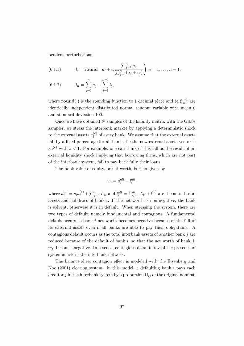
pendent perturbations,

li = round

(ai + εi

∑nj=1 aj∑n

j=1(aj + εj)

), i = 1, . . . , n− 1,(6.1.1)

ln =n∑

j=1

aj −n−1∑

j=1

lj ,(6.1.2)

where round(·) is the rounding function to 1 decimal place and (εi)n−1i=1 are

identically independent distributed normal random variable with mean 0

and standard deviation 100.

Once we have obtained N samples of the liability matrix with the Gibbs

sampler, we stress the interbank market by applying a deterministic shock

to the external assets a(e)i of every bank. We assume that the external assets

fall by a fixed percentage for all banks, i.e the new external assets vector is

sa(e) with s < 1. For example, one can think of this fall as the result of an

external liquidity shock implying that borrowing firms, which are not part

of the interbank system, fail to pay back fully their loans.

The book value of equity, or net worth, is then given by

wi = aalli − lalli ,

where aalli = sia(e)i +

∑nj=1 Lji and lalli =

∑nj=1 Lij + l

(e)i are the actual total

assets and liabilities of bank i. If the net worth is non-negative, the bank

is solvent, otherwise it is in default. When stressing the system, there are

two types of default, namely fundamental and contagious. A fundamental

default occurs as bank i net worth becomes negative because of the fall of

its external assets even if all banks are able to pay their obligations. A

contagious default occurs as the total interbank assets of another bank j are

reduced because of the default of bank i, so that the net worth of bank j,

wj , becomes negative. In essence, contagious defaults reveal the presence of

systemic risk in the interbank network.

The balance sheet contagion effect is modeled with the Eisenberg and

Noe (2001) clearing system. In this model, a defaulting bank i pays each

creditor j in the interbank system by a proportion Πij of the original nominal

97

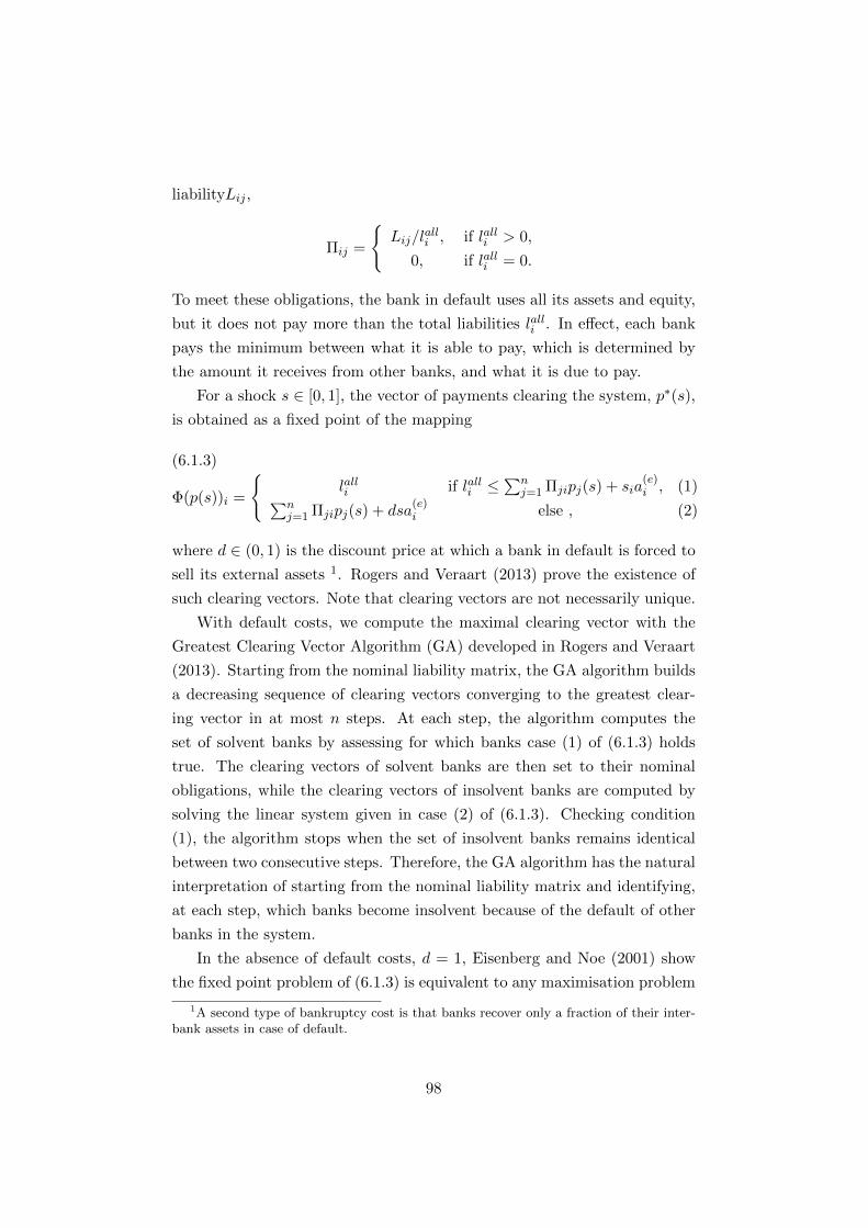
liabilityLij ,

Πij =

Lij/l

alli , if lalli > 0,

0, if lalli = 0.

To meet these obligations, the bank in default uses all its assets and equity,

but it does not pay more than the total liabilities lalli . In effect, each bank

pays the minimum between what it is able to pay, which is determined by

the amount it receives from other banks, and what it is due to pay.

For a shock s ∈ [0, 1], the vector of payments clearing the system, p∗(s),

is obtained as a fixed point of the mapping

Φ(p(s))i =

lalli if lalli ≤

∑nj=1 Πjipj(s) + sia

(e)i , (1)

∑nj=1 Πjipj(s) + dsa

(e)i else , (2)

(6.1.3)

where d ∈ (0, 1) is the discount price at which a bank in default is forced to

sell its external assets 1. Rogers and Veraart (2013) prove the existence of

such clearing vectors. Note that clearing vectors are not necessarily unique.

With default costs, we compute the maximal clearing vector with the

Greatest Clearing Vector Algorithm (GA) developed in Rogers and Veraart

(2013). Starting from the nominal liability matrix, the GA algorithm builds

a decreasing sequence of clearing vectors converging to the greatest clear-

ing vector in at most n steps. At each step, the algorithm computes the

set of solvent banks by assessing for which banks case (1) of (6.1.3) holds

true. The clearing vectors of solvent banks are then set to their nominal

obligations, while the clearing vectors of insolvent banks are computed by

solving the linear system given in case (2) of (6.1.3). Checking condition

(1), the algorithm stops when the set of insolvent banks remains identical

between two consecutive steps. Therefore, the GA algorithm has the natural

interpretation of starting from the nominal liability matrix and identifying,

at each step, which banks become insolvent because of the default of other

banks in the system.

In the absence of default costs, d = 1, Eisenberg and Noe (2001) show

the fixed point problem of (6.1.3) is equivalent to any maximisation problem

1A second type of bankruptcy cost is that banks recover only a fraction of their inter-bank assets in case of default.

98

with a strictly increasing objective function under the constraint that the

clearing vector does not exceed the total inflows, i.e., for each bank i, pi ≤∑nj=1 Πjipj(s) + sia

(e)i . Therefore, we use a linear program to compute the

clearing vectors.

For each bank i affected by contagious default, we estimate the proba-

bility of a contagious default with the average of the occurrence of default

Dti ∈ 0, 1,

P ( Bank i defaults) =1

N

N∑

t=1

Dti .(6.1.4)

Note that fundamentally insolvent banks’ defaults for each sample Lt of

the liability matrix regardless of the individual values of Lt and the default

costs. Moreover, for each bank i, we define the set of samples for which the

bank defaults,

Di = t ∈ 1, . . . , N|Dti = 1.

Then, for each defaulting bank, we compute the Mean Loss Given Default

(MLGD),

MLGD = 1− 1

#Di

∑

t∈Di

pti(s)

lalli,(6.1.5)

wherepti(s)

lalliis the recovery rate of bank i for sample t. For non-defaulting

banks, the MLGD is zero, although their net worth is actually reduced as a

result of other banks’ defaults2.

6.1.2 Choice of the Parameters

Based on the 2011 EBA report, we study the stability and the structure of

two networks. In Section 6.2, the first network consists of n = 11 German

banks with balance sheet information listed in Table D.1; see Appendix D.

2To measure the reduction of a bank equity, one should compute the difference (in networth) between the original net worth assuming all banks are able to pay their nominalliabilities and the net worth resulting from the clearing vectors. Because of limited liability,the value of equity should be set to zero for banks in default; see Rogers and Veraart(2013), Definition 2.9. Therefore, the maximal loss is of 100% and this measure does notdifferentiate defaulting banks.

99

In Section 6.3, the second network consists of n = 76 European banks3 with

balance sheet information listed in Table E.1; see Appendix E.

For the German and the European networks, we apply on each system a

fall in external assets by setting s = 0.97, respectively s = 0.96, and default

costs with d = 0.95, respectively d = 0.96. To study the properties of the

default probability estimator (6.1.4), the magnitude of the shock is chosen

to avoid a binary situation where the default probabilities are either 0 or 1

for all banks.

We now discuss the choice of the parameters for the Gibbs sampler.

We assume that both networks are homogeneous with parameters pij = p,

αij = α, and λij = λ,∀i 6= j ∈ N . As 2n − 1 strictly positive constraints

need to be verified, at least 2n−1 non-diagonal entries of the liability matrix

are required to be strictly positive. As such, we choose the probability of two

banks being connected to be larger that the number of constraints divided

by the number of non-diagonal entries, i.e., p ≥ (2n − 1)/(n2 − n). The

parameters α and λ are chosen such that the expected value of the sum

of the entries equals to the observed total amount of interbank assets or

equivalently to the total amount of interbank liabilities. Let A =∑n

i=i ai,

we have

E

n∑

i=1

n∑

j=1

Lij

=

n∑

i=1

n∑

j=1

pijαijλij

= n(n− 1)pα

λ.

Hence, for a given shape paramater α, we choose the rate parameter λ such

that

λ =pn(n− 1)

Aα.(6.1.6)

Because of numerical considerations, simulations show that we are also con-

strained on the choice of the shape parameter. In the case of the European

network, the normalisation constant of the conditional CDF is extremely

small on certain cycles for large shape parameters, and, as computer preci-

sion is reached, it is rounded down to the value 0. In such cases, we simply

skip the step in the chain and move forward. With the choice of our parame-

3Following Glasserman and Young (2015), we remove, the ten smallest banks, in termsof total assets, from the original EBA data set of 90 European banks. For some smallbanks, balance sheet data are note reliable as reported total assets are smaller than inter-bank assets. Countries with a single reported bank are also excluded.

100

ters, this happens very infrequently. For example, in the European network

with α = 5 and p = 0.9, we reject 3 · 10−3 % of the samples requiring the

normalisation constant to be computed. Nevertheless, the situation becomes

more problematic as both the shape parameter and the edge probability in-

crease. Although these numerical issues show the limitation of the inverse

transform method introduced in Subsection 5.3.1, using a large shape pa-

rameter for the prior distribution is hardly justifiable. Indeed, for the choice

of parameters (6.1.6), the variance of the priori decreases sharply to 0 as the

shape parameter increases4.

In our setting, we also need to carefully choose the number of samples

computed with the Gibbs sampler. Indeed, samples between two steps in the

chain are highly correlated because the Gibbs sampler updates smaller cycles

with a higher probability. In the large European network, the proportion of

entries changed at each step is small and autocorrelation is especially strong.

Therefore, we want to go deep into the chain to ensure that the whole space

is visited. As we cannot keep all the samples in memory, we need to thin

the chain by keeping only every M -th sample. Moreover, it would be too

time consuming to keep all the samples in order to compute the estimators

(6.1.4) and (6.1.5). Although this method increases the variance of the

empirical average, using thinning is justified because we do not lose too

much information by throwing away strongly correlated samples.

Unlike a standard Monte-Carlo method, a central limit theorem for the

chain generated by the Gibbs sampler is not established and we are not able

to formally build confidence intervals for estimators (6.1.4) and (6.1.5). In

particular, the exact rate of convergence of the algorithm is not known. The

following parameters ensure consistent results when sampling from different

seeds5. To control the dependency on the initial liability matrix, we throw

away the first B samples. This is known as the burn-in period. Finally, the

number of samples for the Gibbs sampler is chosen to be N = 10000, with

a burning period B = 10000, respectively 50000, and we thin the chain by

keeping every M = 5000th, respectively 20000th, sample for the German

network, respectively for the European network6.

4Let κ = pn(n−1)A

, the mean of the prior is 1κ

and its variance is equal to 1κ2α

. Thereforethe prior distribution degenerates to a Dirac measure localised at 1

κ, as α→∞.

5For a detailed discussion of convergence diagnosis for the Gibbs sampler; see Robertand Casella (2004).

6The initial matrix of the Markov Chain, verifying the given sum of the rows and

101

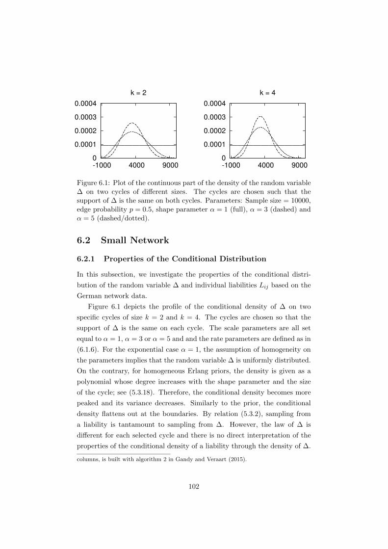
0

0.0001

0.0002

0.0003

0.0004

-1000 4000 9000

k = 2

0

0.0001

0.0002

0.0003

0.0004

-1000 4000 9000

k = 4

Figure 6.1: Plot of the continuous part of the density of the random variable∆ on two cycles of different sizes. The cycles are chosen such that thesupport of ∆ is the same on both cycles. Parameters: Sample size = 10000,edge probability p = 0.5, shape parameter α = 1 (full), α = 3 (dashed) andα = 5 (dashed/dotted).

6.2 Small Network

6.2.1 Properties of the Conditional Distribution

In this subsection, we investigate the properties of the conditional distri-

bution of the random variable ∆ and individual liabilities Lij based on the

German network data.

Figure 6.1 depicts the profile of the conditional density of ∆ on two

specific cycles of size k = 2 and k = 4. The cycles are chosen so that the

support of ∆ is the same on each cycle. The scale parameters are all set

equal to α = 1, α = 3 or α = 5 and and the rate parameters are defined as in

(6.1.6). For the exponential case α = 1, the assumption of homogeneity on

the parameters implies that the random variable ∆ is uniformly distributed.

On the contrary, for homogeneous Erlang priors, the density is given as a

polynomial whose degree increases with the shape parameter and the size

of the cycle; see (5.3.18). Therefore, the conditional density becomes more

peaked and its variance decreases. Similarly to the prior, the conditional

density flattens out at the boundaries. By relation (5.3.2), sampling from

a liability is tantamount to sampling from ∆. However, the law of ∆ is

different for each selected cycle and there is no direct interpretation of the

properties of the conditional density of a liability through the density of ∆.

columns, is built with algorithm 2 in Gandy and Veraart (2015).

102

While each entry has the same unconditional prior distribution, the sup-

port of the conditional posterior density of each off-diagonal liability Lij is

the closed interval between 0 and the minimum of the total interbank lia-

bility li and the total interbank assets aj . For the lower bound 0, we know

that the value zero is sampled from the boundary case of ∆ = ∆low. Note

that, at a specific step in the chain, the liability is not necessarily in the

cycle. Still, it may be equal to zero because it was set to zero the last time

it was part of a cycle. Nevertheless the frequency at which a liability equals

zero measures the dominance of the discrete part of the posterior density.

In Table 6.1, we report properties of the distribution of nine liabilities.

We consider three categories of banks classified by size of interbank assets ai:

the first tercile corresponds to small banks with interbank assets ai ≤ 28000,

the second tercile to medium banks with interbank assets 28000 < ai ≤53000, and the third tercile to large banks with ai > 53000.

In our setting, the effect of the size is particularly strong across the

three categories. The probability of hitting zero for a liability between two

banks of the same category decreases with the size of interbank assets ai.

Liabilities of banks with small, medium and respectively large, interbank

assets are equal to zero with probability 0.94, 0.45, and respectively 0.01.

For liabilities of the type small-large and small-medium, the probability of

liabilities being zero also dominates with value 0.88 and 0.82 respectively.

For liabilities between two banks of the same category, the distributions

of the liability Lij and Lji are similar. This symmetry property between the

distribution of liability Lij and liability Lji extends to liabilities between

banks of different sizes. The distribution of liability Lij shares the same

characteristics as the distribution of Lji both on their discrete and contin-

uous parts, as by (6.1.1), the aggregate amounts of liability and assets are

close to each other. Figure 6.2 illustrates the property of symmetry of the

continuous part of the distribution between banks of different sizes, with L13

corresponding to the liability of bank DE017, with small interbank assets, to

bank DE019, with large interbank assets. Figure 6.2 also confirms that the

continuous part of the density become more peaked as the shape parameter

α increases.

103

,Liability Size Density function Discrete Part Continuous Part

Lij Relation Support P (Lij = 0) Mean Std. Dev. (%)

DE023-25 S-S [0, 4645] 0.94 3259 44DE017-18 M-M [0, 46989] 0.45 8703 52DE019-20 L-L [0, 91314] 0.01 25360 41

DE017-25 M-S [0, 4645] 0.88 3777 33DE025-17 S-M [0, 4841] 0.88 3923 33

DE019-25 L-S [0, 4645] 0.82 3966 29DE025-19 S-L [0, 4841] 0.83 4107 30

DE017-19 M-L [0, 46989] 0.20 12430 49DE019-17 L-M [0, 47102] 0.19 12380 50

Table 6.1: Characteristics of the liabilities distribution. The first columncorresponds to the liability Lij . The second columns indicates size of inter-bank assets for bank i and bank j, L = Large, M = Medium, S = Small.The third columns corresponds to the support of the distribution of Lij .The fourth column reports the empirical probability of hitting the bound-ary case zero. The fourth and fifth columns report the mean and the relativestandard deviation of the sample. Parameters: Sample size = 10000, edgeprobability p = 0.5 , shape parameter α = 3.

0

5e-05

0.0001

0 20000 40000

Liability L13

0

5e-05

0.0001

0 20000 40000

Liability L31

Figure 6.2: Plot of the continuous part of the density of liabilities L13 andL31 for different values of the shape parameter α.Parameters: Sample size= 10000, edge probability p = 0.5, α = 2 (full) , α = 3.5 (dashed), α = 5.(dashed/dotted).

104

Bank Bank CTA Mean degree Default without cost Default with costCode Size Ratio(%) in out MLGD (%) Proba MLGD (%) Proba

Fundamental default

DE017 M 1.59 5.05 5.02 1.36 1 6.23 1DE022 M 1.74 5.29 5.28 0.60 1 5.04 1DE023 S 1.69 2.83 2.84 1.27 1 6.15 1DE024 S 2.20 4.14 4.13 0.46 1 5.17 1

Contagious default

DE019 L 2.62 5.96 5.95 0 0 4.02 0.93DE020 L 2.26 6.19 6.20 1.13·10−3 0.03 4.18 0.96DE025 S 2.94 2.32 2.35 4.64·10−3 0.09 4.94 0.82DE028 M 2.58 4.48 4.47 3.90·10−5 0.002 4.00 0.90

No default

DE018 L 3.47 5.15 5.16DE021 L 3.64 5.55 5.57DE027 S 3.86 4.34 4.33

Table 6.2: Characteristics of the banks in the German network. The thirdcolumns corresponds to the capital to total assets (CTA) ratio. The fourthand fifth columns represent the mean number of interbank liabilities andassets respectively. Parameters: Sample size = 10000, edge probability p =0.5 , shape parameter α = 1, shock s = 0.97, default cost d = 0.95.

6.2.2 Stress Test

To understand the likelihood of default in the case of no default costs, we

have to take into account the capital to total assets ratio (CTA) and the

connectivity to the network of the bank. In Table 6.2, Bank DE025 has the

largest CTA among defaulting banks. Nevertheless it has the largest default

probability because it is exposed to 2.32 banks on average and its mean

exposure to fundamentally insolvent banks represents 99% of its total expo-

sure7. Furthermore, bank DE020 is well connected and it has the smallest

CTA ratio among banks affected by contagious default. As such its equity

buffer is not able to absorb external shocks. In particular, it has a higher

probability of default compared to Bank DE019, which has a higher CTA,

although both banks share the same characteristics in terms of connectivity

and size of interbank assets. Hence, the connectivity helps to reduce the

exposure to banks in default, as long as there is enough capital to absorb

the reduction in expected payments from a single default.

When default costs are incorporated, the propagation of defaults be-

comes wider and deeper. The loss of 5% on the sell of external assets in-

7Note that if a bank is exposed mainly to defaulting banks, connectivity may actuallyincrease its probability of default.

105

creases by one thousand fold the size of default and by ten fold the default

probability of banks suffering from contagious default. Compared to the no

cost case, these larger LGDs result into an additional bank exposed to a high

default probability. As only banks with proportionally large equity buffer

are able to cover their losses, the CTA is a good indicator of resilience. Fun-

damentally insolvent banks have a CTA between 1.59% and 2.20%. Banks

affected by contagious default have a CTA between 2.26% and 2.94%, and

non-defaulting banks have a CTA between 3.47% and 3.86%.

We now discuss the effect of the shape parameter on the default probabil-

ity for three different shape parameters, α = 1, 3, 5. Figure 6.3 shows that,

with no default costs, the default probability decreases with the connected-

ness of the network. As the network becomes more connected, the losses are

evenly spread through the system and bank net worths are large enough to

absorb the external shock. Furthermore, bank DE025 has the largest default

probability across all shape parameters. Similarly to its mean out-degrees,

Bank DE025 probability of default becomes concave as the shape parameter

increases. For α = 5, the default probability is essentially flat on the interval

p ∈ [0.2, 0.5], it is then reduced significantly as the number of out-degrees,

or equivalently of in-degrees, increases; see Figure 6.4.

For banks DE020 and DE028, the default probability becomes more

sensitive to the edge probability as the shape parameter increases. Although

every default probability converges to zero, bank DE028 is the most sensitive

to p for all shape parameters. By Table D.1, bank DE028 has smallest net

worth compared to bank DE020 and DE025. In a sparse network, it is

affected by the default of the group of banks in Table 6.2 as losses due to

fundamental defaults are shared only by a few banks. In effect, bank DE028

equity buffer (net worth) is not large enough to prevent it from defaulting.

As the network becomes more connected, the losses are absorbed by more

banks and, because of its relatively hight CTA, the likelihood of default is

reduced efficiently.

As shown in Table 6.2, incorporating default costs changes fundamentally

the outcome of the stress test. Figure 6.3 illustrates that best case scenarios

with no default costs become worst case scenarios with default costs. Indeed,

with no cost, bank DE025 has the highest probability of default among banks

affected by contagious defaults, while it is the least likely bank to default

in the presence of default costs. Moreover, the curvature of its default

106

probability as a function of the edge probability increases with the shape

parameter.

6.2.3 Structure of the Small Network

Regarding the overall structure of the network, we find that mean out and in-

degree are essentially the same; see Table 6.2. Because interbank liabilities

are built as perturbations of interbank assets by (6.1.1), the structure of

interbank assets and liabilities is symmetric for a given bank.

We now study the effect of the shape parameter on the structure of the

network. As in the previous subsection, we choose three different values

of the shape parameter, α = 1, 3, 5, and their associated rate parameters.

Figure 6.4 shows that large banks are the most connected with at least

4 banks with an edge probability p = 0.2 and the number of mean out-

degrees increases at a steady rate for all shape parameters. For a fixed

edge probability p, increasing the shape parameter significantly reduces, the

connectivity of each small bank. In Figure 6.4, small banks face a reduction

of 33% of mean out-degrees on average. For medium and large banks, the

choice of the prior has less impact with a reduction of 11% for medium banks

and an increase of 2% in mean out-degrees for large banks. Furthermore,

the mean out-degree of each small bank shifts downwards for all values of p,

while the difference in mean out-degrees may change sign as p increases for

medium and large banks. Note that, in this example, banks suffering from

contagious default are more sensitive to the choice of the prior.

For the minimal value of the edge probability p = 0.2, the network is

strongly sparse regardless of the choice of the prior. As a result, the prior

does not affect significantly the value of mean out-degrees. When the edge

probability is in the interval p ∈ [0.5, 0.7], the choice of the shape parameter

results in a strong heterogeneous network. Such values of p allow for more

variability across edge realisations and the choice of the prior changes the

network structure at the local and global level. For example, at p = 0.7,

there is a difference of 4 out-degrees between bank DE020 and DE025 for

α = 1 and a difference of 7 for α = 5. Finally, all banks connect as the edge

probability is set to p = 1.

While the effect of the prior of small banks connectivity by concentrating

the exposure to fewer banks for the same prior edge probability, large banks

connectivity is less sensitive to the choice of the prior. This effect can be

107

explained by the fact that the discrete part of the posterior distribution,

which corresponds to the value 0, is dominant for small banks and any

change on the discrete part is directly reflected on the number of mean

out-degrees.

6.3 Large Network

6.3.1 Stress test

In terms of banks’ interbank assets, the European network in Table E.1

has a larger variability than the German network. As such, our aim is to

understand whether the structure and the stability of the network is affected

by its size and its heterogeneity. Furthermore, our interest lies also in the

verification of the performance of the Gibbs sampler on a large network.

Similarly to the German network, we classify banks by size of interbank

assets ai. In the first tercile, ai ≤ 7602, there are 26 banks, in second tercile,

7602 < ai ≤ 34983, and third tercile, ai > 34983, there are respectively 25

banks. On average, the CTA ratio decrease with the size group, with a CTA

of 4.87, 4.20, and 3.54, for small, medium and large banks. Therefore, the

external shock of 4%, s = 0.96 on the system results in more fundamentally

insolvent medium and large banks, with 5 small banks, 9 medium banks, and

12 large banks. Furthermore, similarly to the German network, fundamental

defaults have the largest MLGDs.

In Table 6.3, we report the characteristics of 9 banks, which are either

fundamentally insolvent, affected by contagious default, or non-defaulting.

As discussed above, fundamentally insolvent banks DE017 and IE037 default

because of their low CTA. Although Bank ES069 has a larger CTA than

banks DE017 and IE037, it is fundamentally insolvent because 97% of its

exposure is on external assets. As a result, bank ES069 is more sensitive

to a shock on its external assets than banks with similar CTA, such as

the fundamentally solvent bank IE039 that has an exposure of 85% on its

external assets.

Banks ES067, ES076, IE039 suffer from contagious default. In the stress

test with shock s = 0.96 and with no cost, they have significantly higher

default probabilities and MLGD’s than similar banks in the stressed German

network with a shock s = 0.97. As such, we see that, for the same edge

probability p = 0.5, the large size of the network is not able to absorb

108

a stronger shock of 1%, although it should facilitate the spread of losses

across banks. In this aspect, the behavior of the default probability of bank

ES076 demonstrates that neither the size nor the connectivity of the network

necessarily helps to reduce the probability of default. Indeed, Figure 6.5

shows that its probability of default increases with the edge probability p

regardless of the choice of the prior in the no cost case. While its size of

default is small compared to other defaulting banks, the likelihood is high as

it has significantly more exposure to the interbank asset in terms of assets

to total assets ratio, namely 63.65% compared to 40.20% and 13.11% for

banks ES067 and IE039. When default costs are incorporated, the size of

default is the same for both networks, since default costs cannot be shared

through the network.

The choice of the prior has different effects on the default probability

affected by contagious defaults. In the no cost case, increasing the shape

parameter increases the slope of the default probability profile for bank

ES076. For banks ES067 and IE039, the probability of default decrease

with p, while starting from a slightly higher default probability at p = 0.2.

With default costs, increasing the shape parameter has no significant impact

on the default probability of bank ES067 and bank IE039, while it reduces

the default probability of bank ES076.

Bank Bank CTA Mean degree Default without cost Default with costCode Size Ratio(%) in out MLGD (%) Proba MLGD (%) Proba

Fundamental default

DE017 L 1.59 38.77 38.74 2.09 1 5.78 1ES069 S 3.59 11.26 11.06 0.31 1 4.17 1IE037 M 2.79 21.62 21.78 0.95 1 4.70 1

Contagious default

ES067 S 3.89 12.87 13.09 0.39 0.002 3.40 0.88ES076 S 3.76 10.50 10.34 0.07 0.49 3.81 0.98IE039 S 3.60 17.35 17.50 0.05 0.007 3.54 0.97

No default

DK009 S 5.19 15.56 15.91GB091 M 4.77 29.02 29.09IT040 L 4.53 37.12 37.02

Table 6.3: Characteristics of the banks in the European network. The thirdcolumns corresponds to the capital to total assets (CTA) ratio. The fourthand fifth columns represent the mean number of interbank liabilities andassets respectively. Parameters. Sample size = 10000, edge probabilityp = 0.5 , shape parameter α = 1, shock s = 0.96, default cost d = 0.96.

109

6.3.2 Structure of the Large Network

The structure of the European network shares the same characteristics with

the German network. Because of assumption (6.1.1) on the vector to total

liabilities, the network is symmetric and the mean out and in-degrees are

essentially the same. Similarly to the German network, Figure 6.6 shows

that the choice of the prior has a strong influence on the connectivity of

small banks. Reported banks suffering from contagious banks are all small

banks and we observe a reduction of 50% in mean out-degrees from α = 1

to α = 3. Moreover, for large banks, we also find that the difference in mean

out-degrees for two different priors may change sign as the edge probability

p increases. For example, bank DE017 has 28% more out-degrees at p = 0.2

and 8% less out-degrees at p = 0.9. Hence, the assumption of homogeneous

prior edge probability show that our sampling method which is determined

by the size of interbank assets and liabilities reflects the expected tiered

structure of interbank networks, with larger banks, being more connected.

Finally, the dominance of the discrete part of the posterior distribution in-

creases with the shape parameter, and, as a result, small banks are especially

sensitive to the choice of the prior.

6.4 Conclusion

We have developed a new method for sampling from the joint distribution

of liabilities conditionally on the given sum of the nominal interbank assets

and liabilities of each bank. Our method allows for general Gamma density

functions on the continuous part of the liabilities. At each step of the Gibbs

sampler, the sampling of the joint distribution reduces to sample of a one

dimensional random variable ∆ by selecting an appropriate submatrix. Un-

der the assumption of a homogeneous network and natural scale parameters,

we obtain a closed form solution for the CDF and we sample from the law

using an inverse transform method.

Based on a network of 11 banks, we show that, for the same prior, our

sampling method results in a fully heterogeneous network at each sample.

The continuous part of the posterior distributions have different means and

variances and the size of the assets is determinant for the dominance of

the discrete part over the continuous part of the density. Similarly, the

properties of the default probability and connectivity of each bank are also

110

determined by the size of interbank assets. In particular, the structure of

small banks is especially sensitive to the the choice of the prior.

Our empirical study of the European network of 76 banks shows that

the Gibbs sampler also operates on large networks at the cost of using a

large thinning. Our empirical results demonstrate that the profile of default

probabilities is different for banks of the same size and we exhibit an example

of a bank whose default probability always increases with the prior edge

probability. This serves as empirical example that a more connected network

does not necessarily reduce the spread of contagious defaults. Finally, we

show that the structure of the large European network obtained with our

sampling method is similar to the structure of the smaller German network.

111

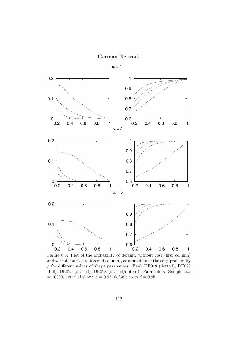
German Network

α = 1

0

0.1

0.2

0.2 0.4 0.6 0.8 1

0.6

0.7

0.8

0.9

1

0.2 0.4 0.6 0.8 1

α = 3

0

0.1

0.2

0.2 0.4 0.6 0.8 1

0.6

0.7

0.8

0.9

1

0.2 0.4 0.6 0.8 1

α = 5

0

0.1

0.2

0.2 0.4 0.6 0.8 1

0.6

0.7

0.8

0.9

1

0.2 0.4 0.6 0.8 1

Figure 6.3: Plot of the probability of default, without cost (first column)and with default costs (second column), as a function of the edge probabilityp for different values of shape parameters. Bank DE019 (dotted), DE020(full), DE025 (dashed), DE028 (dashed/dotted). Parameters: Sample size= 10000, external shock, s = 0.97, default costs d = 0.95.

112

German Network

3 5 7 9

0.2 0.4 0.6 0.8

α = 1

5 7 9

0.2 0.4 0.6 0.8

α = 3

5 7 9

0.2 0.4 0.6 0.8

α = 5

3

5

7

9

0.2 0.4 0.6 0.8

3

5

7

9

0.2 0.4 0.6 0.8

1

3

5

7

9

0.2 0.4 0.6 0.8

Banks in fundamental default: DE017 (dotted), DE022 (full), DE023(dashed), Bank DE024 (dashed/dotted)

3

5

7

9

0.2 0.4 0.6 0.8

1

3

5

7

9

0.2 0.4 0.6 0.8

1

3

5

7

9

0.2 0.4 0.6 0.8

Banks in contagious default: DE019 (dotted), DE020 (full), DE025(dashed), DE028 (dashed/dotted)

3

5

7

9

0.2 0.4 0.6 0.8

3

5

7

9

0.2 0.4 0.6 0.8

3

5

7

9

0.2 0.4 0.6 0.8

Non-Defaulting Banks: DE018 (full), Bank DE021 (dashed), DE027(dashed/dotted)

Figure 6.4: Plot of the mean out-degree of bank j, E(∑

j Aij |a, l), as afunction of the edge probability p for different values of shape parameters.Parameters: Sample size = 10000, external shock, s = 0.97, default costsd = 0.95.

113

European Networkα = 1

0

0.1

0.2

0.3

0.4

0.5

0.6

0.7

0.2 0.4 0.6 0.8 1

0.7

0.8

0.9

1

0.2 0.4 0.6 0.8 1

α = 3

0

0.1

0.2

0.3

0.4

0.5

0.6

0.7

0.2 0.4 0.6 0.8 1

0.7

0.8

0.9

1

0.2 0.4 0.6 0.8 1

α = 5

0

0.1

0.2

0.3

0.4

0.5

0.6

0.7

0.2 0.4 0.6 0.8 1

0.7

0.8

0.9

1

0.2 0.4 0.6 0.8 1

Figure 6.5: Plot of the probability of default, without cost (first column) andwith default costs (second column), as a function of the edge probability pfor different values of shape parameters. Parameters: Sample size = 10000,external shock, s = 0.96, default costs d = 0.96. Bank ES067 (full), ES076(dashed), IE039 (dashed/dotted).

114

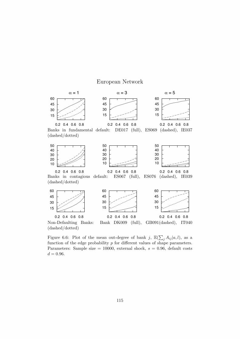
European Network

3 5 7 9

0.2 0.4 0.6 0.8

α = 1

5 7 9

0.2 0.4 0.6 0.8

α = 3

5 7 9

0.2 0.4 0.6 0.8

α = 5

15

30

45

60

0.2 0.4 0.6 0.8

15

30

45

60

0.2 0.4 0.6 0.8

15

30

45

60

0.2 0.4 0.6 0.8

Banks in fundamental default: DE017 (full), ES069 (dashed), IE037(dashed/dotted)

10

20

30

40

50

0.2 0.4 0.6 0.8

10

20

30

40

50

0.2 0.4 0.6 0.8

10

20

30

40

50

0.2 0.4 0.6 0.8

Banks in contagious default: ES067 (full), ES076 (dashed), IE039(dashed/dotted)

15

30

45

60

0.2 0.4 0.6 0.8

15

30

45

60

0.2 0.4 0.6 0.8

15

30

45

60

0.2 0.4 0.6 0.8

Non-Defaulting Banks: Bank DK009 (full), GB091(dashed), IT040(dashed/dotted)

Figure 6.6: Plot of the mean out-degree of bank j, E(∑

j Aij |a, l), as afunction of the edge probability p for different values of shape parameters.Parameters: Sample size = 10000, external shock, s = 0.96, default costsd = 0.96.

115

Appendix D

Balance Sheet: German

Network

Bank Code Name Total Assets Interbank Assets Tier 1 Capital

a+ a(e) a w

DE017 DEUTSCHE BANK AG 1,905,630 47,102 30,361DE018 COMMERZBANK AG 771,201 49,871 26,728DE019 LANDESBANK BADEN-WURTTEMBERG 374,413 91,201 9,838DE020 DZ BANK AG 323,578 100,099 7,299DE021 BAYERISCHE LANDESBANK 316,354 66,535 11,501DE022 NORDDEUTSCHE LANDESBANK -GZ- 228,586 54,921 3,974DE023 HYPO REAL ESTATE HOLDING AG 328,119 7,956 5,539DE024 WESTLB AG, DUSSELDORF 191,523 24,007 4,218DE025 HSH NORDBANK AG, HAMBURG 150,930 4,645 4,434DE027 LANDESBANK BERLIN AG 133,861 27,707 5,162DE028 DEKABANK DEUTSCHE GIROZENTRAL 130,304 30,937 3,359

Table D.1: Balance sheet information of 11 German banks provided for the2011 EBA stress test. All quantities are in million euros.

116

Appendix E

Balance Sheet: European

Network

117

Bank Code Name Total Assets Interbank Assets Tier 1 Capitala+ a(e) a w

AT001 Erste Bank Group (EBG) 205938 25044 10507AT002 Raiffeisen Bank International (RBI) 131173 30361 7641AT003 Oesterreichische Volksbank AG 44745 10788 1765BE004 DEXIA 548135 228211 17002BE005 KBC BANK 276723 23871 11705CY006 MARFIN POPULAR BANK PUBLIC CO LT 42580 7907 2015CY007 BANK OF CYPRUS PUBLIC CO LTD 41996 7294 2134DE017 DEUTSCHE BANK AG 1905630 194399 30361DE018 COMMERZBANK AG 771201 138190 26728DE019 Landesbank Baden-Wrttemberg 374413 133906 9838DE020 DZ BANK AG Dt. Zentral-Genoss. 323578 135860 7299DE021 Bayerische Landesbank 316354 97336 11501DE022 Norddeutsche Landesbank -GZ 228586 91217 3974DE023 Hypo Real Estate Holding AG 328119 29084 5539DE024 WestLB AG Dsseldorf 191523 58128 4218DE025 HSH Nordbank AG Hamburg 150930 9532 4434DE027 Landesbank Berlin AG 133861 49253 5162DE028 DekaBank Deutsche Girozentrale Franl 130304 41255 3359DK008 DANSKE BANK 402555 75894 14576DK011 Nykredit 175888 8597 6633DK009 Jyske Bank 32752 4674 1699DK010 Sydbank 20238 3670 1231ES059 BANCO SANTANDER S.A. 1223267 51407 41998ES060 BANCO BILBAO VIZCAYA ARGENTARIA 540936 110474 24939ES061 BFA-BANKIA 327930 39517 13864ES062 CAJA DE AHORROS Y PENSIONES 275856 5510 11109ES064 BANCO POPULAR ESPANOL S.A. 129183 14810 6699ES065 BANCO DE SABADELL S.A. 96703 3678 3507ES066 CAIXA DESTALVIS DE CATALUNYA 76014 8219 3104ES067 CAIXA DE AFORROS DE GALICIA 73319 2948 2849ES083 CAJA DE AHORROS DEL MEDITERRANEO 72034 4981 1843ES071 GRUPO BANCA CIVICA 71055 7419 3688ES068 GRUPO BMN 69760 7660 3304ES063 EFFIBANK 54523 4124 2656

(continued on next page)

118

Bank Code Name Total Assets Interbank Assets Tier 1 Capitala+ a(e) a w

ES069 BANKINTER S.A. 53476 2141 1920ES070 CAJA ESPANA DE INVERSIONES SALAMANCA 45656 7235 2076ES075 GRUPO BBK 44628 1924 2982ES072 CAJA DE AHORROS Y M.P. DE ZARAGOZ 42716 1779 2299ES073 MONTE DE PIEDAD Y CAJA DE AHORRO 34263 2599 2501ES074 BANCO PASTOR S.A. 31135 1665 1395ES076 CAIXA DESTALVIS UNIO DE CAIXES DE... 28310 1802 1065ES077 CAJA DE AHORROS Y M.P. DE GIPUZKO 20786 285 1935ES078 GRUPO CAJA3 20144 1926 1164FR013 BNP PARIBAS 1998157 90328 55352FR014 CREDIT AGRICOLE 1503621 83713 46277FR016 SOCIETE GENERALE 1051323 100013 27824FR015 BPCE 1000695 34983 31943GB089 HSBC HOLDINGS plc 1783199 212092 86900GB090 BARCLAYS plc 1725709 53873 46232GB091 LLOYDS BANKING GROUP plc 1006082 29233 47984GB088 ROYAL BANK OF SCOTLAND GROUP plc 607351 105506 58982GR031 NATIONAL BANK OF GREECE 118832 8608 8153GR030 EFG EUROBANK ERGASIAS S.A. 85885 3838 4296GR032 ALPHA BANK 66798 3492 5275GR033 PIRAEUS BANK GROUP 57680 1581 3039GR034 AGRICULTURAL BANK OF GREECE S.A. 31221 1657 792IE038 BANK OF IRELAND 156712 17254 7037IE037 ALLIED IRISH BANKS PLC 131311 11277 3669IE039 IRISH LIFE AND PERMANENT 46743 6127 1681IT041 UNICREDIT S.p.A 929488 106707 35702IT040 INTESA SANPAOLO S.p.A 576962 109909 26159IT042 BANCA MONTE DEI PASCHI DI SIENA 244279 12074 6301IT043 BANCO POPOLARE S.C. 140043 7602 5474IT044 UNIONE DI BANCHE ITALIANE SCPA 130559 19793 6559NL047 ING BANK NV 933073 111756 30895NL048 RABOBANK NEDERLAND 607483 37538 27725NL049 ABN AMRO BANK NV 379599 29196 11574NL050 SNS BANK NV 78918 388 1782PT053 CAIXA GERAL DE DEPSITOS SA 119318 14221 6510PT054 BANCO COMERCIAL PORTUGUS SA 100010 7690 3521PT055 ESPRITO SANTO FINANCIAL GROUP 85644 8690 4520PT056 Banco BPI SA 43826 5463 2133SE084 Nordea Bank AB 542853 61448 19103SE085 Skandinaviska Enskilda Banken AB 212240 25955 9604SE086 Svenska Handelsbanken AB 240202 20870 8209SE087 Swedbank AB 191365 17358 7352

Figure E.1: Balance sheet information of 76 European banks system forthe 2011 EBA stress test. The data is provided in Glasserman and Young(2015). All quantities are in million euros.

119

Bibliography

Acemoglu, D., Ozdaglar, A., and Tahbaz-Salehi, A. (2015). Systemic

risk and stability in financial networks. American Economic Review,

105(2):564–608.

Acharya, V. V. and Yorulmazer, T. (2008). Cash-in-the-market pricing

and optimal resolution of bank failures. Review of Financial Studies,

21(6):2705–2742.

Allen, F. and Gale, D. (2000). Financial contagion. Journal of political

economy, 108(1):1–33.

Bach, F., Ahipasaoglu, S. D., and d’Aspremont, A. (2010). Convex relax-

ations for subset selection. Technical report Arxiv 1006-3601.

Bauerle, N., Urban, S. P., and Veraart, L. A. M. (2013). The relaxed in-

vestor with partial information. SIAM Journal on Financial Mathematics,

3(1):304–327.

Benoit, S., Colliard, J.-E., Hurlin, C., and Perignon, C. (2015). Where

the risks lie: a survey on systemic risk. Available at SSRN:

http://ssrn.com/abstract=2577961.

Best, M. J. and Grauer, R. R. (1991). On the sensitivity of mean-variance-

efficient portfolios to changes in asset means: Some analytical and com-

putational results. The Review of Financial Studies, 4(2):315–342.

Brandt, M. W. (2010). Portfolio choice problems. In Hanbook of financial

econometrics, volume 1: tools and techniques, volume 1, 269–336. North

Holland.

Brodie, J., Daubechies, I., De Mol, C., Giannone, D., and Loris, I. (2009).

Sparse and stable Markowitz portfolios. PNAS, 106(30):12267–12272.

120

Brunnermeier, M. K. and Oehmke, M. (2013). Bubbles, Financial Crises,

and Systemic Risk. Elsevier, Amsterdam.

Chan, L. K. C., Karceski, J., and Lakonishok, J. (1999). On portfolio op-

timization: Forecasting covariances and choosing the risk model. The

Review of Financial Studies, 12(5):937–974.

Chen, N., Liu, X., and Yao, D. D. (2014). An optimization view of fi-

nancial systemic risk modeling: The network effect and the market liq-

uidity effect. Available at SSRN: http://ssrn.com/abstract=2463545 or

http://dx.doi.org/10.2139/ssrn.2463545.

Chopra, V. K. (1993). Improving optimization. The Journal of Investing,

2(3):51–59.

Cocco, J. F., Gomes, F. J., and Martins, N. C. (2009). Lending relationships

in the interbank market. Journal of Financial Intermediation, 18(1):24–

48.

Cont, R., Moussa, A., and Santos, E. B. (2013). Network structure and

systemic risk in banking systems. Handbook on Systemic Risk, 1:327–336.

Cvitanic, J. and Karatzas, I. (1992). Convex duality in constrained portfolio

optimization. The Annals of Applied Probability, 2(4):767–818.

Davis, M. H. A. and Norman, A. R. (1990). Portfolio selection with trans-

action costs. Mathematics of Operations Research, 15(4):676–713.

De Bandt, O., Hartmann, P., and Peydro, J. L. (2009). Systemic risk in

banking an update. The Oxford Handbook of Banking.

Degryse, H. and Nguyen, G. (2007). Interbank exposures: An empirical ex-

amination of contagion risk in the Belgian banking system. International

Journal of Central Banking, 3(2):123–171.

DeMiguel, V., Garlappi, L., Nogales, F., and Uppal, R. (2009a). A gen-

eralized approach to portfolio optimization: Improving performance by

constraining portfolio norms. Management Science, 55(5):15.

DeMiguel, V., Garlappi, L., and Uppal, R. (2009b). Optimal versus naive

diversification: How inefficient is the 1/N portfolio strategy? Review of

Financial Studies, 22(5):1915–1953.

121

Donoho, L. and Johnstone, I. M. (1994). Ideal spatial adaptation by wavelet

shrinkage. Biometrika, 81(3):425–455.

Efron, B., Hastie, T., Johnstone, I., and Tibshirani, R. (2004). Least angle

regression. The Annals of Statistics., 32(2):407–451.

Eisenberg, L. and Noe, T. H. (2001). Systemic risk in financial systems.

Management Science, 47(2):236–249.

El Karoui, N. (2010). High-dimensionality effects in the markowitz problem

and other quadratic programs with linear constraints: Risk underestima-

tion. The Annals of Statistics, 38(6):3487–3566.

Elsinger, H., Lehar, A., and Summer, M. (2006). Using market informa-

tion for banking system risk assessment. International Journal of Central

Banking, 2(1).

Elsinger, H., Lehar, A., and Summer, M. (2013). Network models and

systemic risk assessment. Handbook on Systemic Risk, 1:287–305.

Erdos, P. and Renyi, A. (1959). On random graphs I. Publicationes Mathe-

maticae Debrecen, 6:290–297.

Fama, E. F. and French, K. R. (1993). Common risk factors in the returns

of stocks and bonds. Journal of Financial Economics, 107:3–56.

Fan, J., Zhang, J., and Yu, K. (2012). Vast portfolio selection with gross-

exposure constraints. Journal of the American Statistical Association,

107(498):592–606.

Farhi, E. and Tirole, J. (2012). Collective moral hazard, maturity mismatch,

and systemic bailouts. American Economic Review, 102(1):60–93.

Freixas, X., Parigi, B. M., and Rochet, J.-C. (2000). Systemic risk, interbank

relations, and liquidity provision by the central bank. Journal of Money,

Credit and Banking, 32(3):pp. 611–638.

Frost, P. A. and Savarino, J. E. (1988). For better performance: Constrain

portfolio weights. The Journal of Portfolio Management, 15(1):29–34.

Furfine, C. H. (2003). Interbank exposures: quantifying the risk of contagion.

Journal of money, credit and banking, 111–128.

122

Gandy, A. and Veraart, L. A. M. (2013). The effect of estimation in high-

dimensional portfolios. Mathematical Finance, 23(3):531–559.

Gandy, A. and Veraart, L. A. M. (2015). A Bayesian methodology for

systemic risk assessment in financial networks. Available at SSRN:

http://ssrn.com/abstract=2580869.

Glasserman, P. (2004). Monte Carlo Methods in Financial Engineering.

Springer, 1 edition.

Glasserman, P. and Young, H. P. (2015). How likely is contagion in financial

networks? Journal of Banking & Finance, 50:383–399.

Goldstein, M. A., Irvine, P., Kandel, E., and Wiener, Z. (2009). Brokerage

Commissions and Institutional Trading Patterns. Review of Financial

Studies, 22(12):5175–5212.

Green, R. and Hollifield, B. (1992). When will mean-variance efficient port-

folios be well-diversified? Journal of Finance, 47(5):1785–1809.

Haldane, A. G. (2009). Rethinking the financial network,april 2009.speech

delivered at the financial student association, amsterdam.

Jagannathan, R. and Ma, T. (2003). Risk reduction in large portfolios: Why

imposing the wrong constraints helps. Journal of Finance, 58(4):1651–

1684.

James, W. and Stein, C. (1961). Estimation with quadratic loss. In Proc.

Fourth Berkeley Symp. on Math. Statist. and Prob., Vol. 1 (Univ. of Calif.

Press), 361–379.

Jobson, J. D. and Korkie, B. (1980). Estimation for markowitz efficient

portfolios. Journal of the American Statistical Association, 75(371):544–

554.

Jobson, J. D. and Korkie, B. (1981). Putting markowitz theory to work.

Journal of the American Statistical Association, 7(4):70–74.

Jorion, P. (1986). Bayes-Stein estimation for portfolio analysis. Journal of

Financial and Quantitative Analysis, 21(3):279–292.

123

Kan, R. and Zhou, G. (2007). Optimal portfolio choice with parameter

uncertainty. Journal of Financial and Quantitative Analysis, 42(3):621–

656.

Karatzas, I. and Shreve, S. (1998). Methods of mathematical finance. New

York: Springer-Verlag.

Keim, D. B. and Madhavan, A. (1998). The cost of institutional equity

trades. Financial Analysts Journal, 54(4):50–69.

Kempf, A., Korn, O., and Sassning, S. (2015). Portfolio optimization using

forward-looking information. Review of Finance, 19(1):467–490.

Ledoit, O. and Wolf, M. (2004a). Honey, I shrunk the sample covariance

matrix. Journal of Portfolio Management, 30(4):110–119.

Ledoit, O. and Wolf, M. (2004b). A well-conditioned estimator for

large-dimensional covariance matrices. Journal of Multivariate Analysis,

88(2):365 – 411.

Lee, G. M., Tam, N. N., and Yen, N. D. (2006). Continuity of the solu-

tion map in quadratic programs under linear perturbations. Journal of

Optimization Theory and Applications, 129(3):415–423.

Levy, H. and Markowitz, H. M. (1979). Approximating expected utility

by a function of mean and variance. The American Economic Review,

69(3):308–317.

Luenberger, D. G. (1969). Optimization by vector space methods. John

Wiley & Sons.

Markowitz, H. M. (1952). Portfolio selection. Journal of Finance, 7(1):77–

91.

Merton, R. C. (1971). Optimum consumption and portfolio rules in a

continuous-time model. Journal of Economic Theory, 3(4):373–413.

Merton, R. C. (1973). An inter temporal capital asset pricing model. Econo-

metrica, 41:867–887.

Merton, R. C. (1980). On estimating the expected return on the market: An

exploratory investigation. Journal of Financial Economics, 8(4):323–361.

124

Michaud, R. O. (1989). The markowitz optimization enigma: Is ’optimized’

optimal? Financial Analysts Journal, 45(1):31–42.

Mistrulli, P. E. (2011). Assessing financial contagion in the interbank mar-

ket: Maximum entropy versus observed interbank lending patterns. Jour-

nal of Banking & Finance, 35(5):1114–1127.

Moreau, J. J. (1965). Proximite et dualite dans un espace hilbertien. Bulletin

de la S.M.F, 93:273–299.

Natarajan, B. K. (1995). Sparse approximate solutions to linear systems.

SIAM Journal on Computing, 24(2):227–234.

Nier, E., Yang, J., Yorulmazer, T., and Alentorn, A. (2007). Network mod-

els and financial stability. Journal of Economic Dynamics and Control,

31(6):2033–2060.

Osborne, M. R., Presnell, B., and Turlach, B. A. (2000). On the lasso and

its dual. Journal of Computational and Graphical Statistics, 9(2):319–337.

Pham, H. (2009). Continuous-time stochastic control and optimization with

financial applications. Springer.

Piessens, R., de Doncker-Kapenga, E., Uberhuber, C. W., and Kahaner,

D. K. (1983). QUADPACK: A subroutine package for automatic integra-

tion. Springer, 1 edition.

Robert, C. and Casella, G. (2004). Monte Carlo statistical methods.

Springer, 2 edition.

Rogers, L. C. G. (2001). The relaxed investor and parameter uncertainty.

Finance and Stochastics, 5(2):131–154.

Rogers, L. C. G. and Veraart, L. A. M. (2013). Failure and rescue in an

interbank network. Management Science, 59(4):882–898.

Roll, R. and Ross, S. A. (1980). An empirical investigation of the arbitrage

pricing theory. The Journal of Finance, 35(5):1073–1103.

Sharpe, W. F. (1964). Capital asset prices: A theory of market equilibrium

under conditions of risk. The Journal of Finance, 19(3):425–442.

125

Tibshirani, R. (1996). Regression shrinkage and selection via the lasso.

Journal of the Royal Statistical Society. Series B, 58(1):267–288.

Tu, J. and Zhou, G. (2011). Markowitz meets Talmud: A combination of

sophisticated and naive diversification strategies. Journal of Financial

Economics, 99(1):204–215.

Upper, C. (2011). Simulation methods to assess the danger of contagion in

interbank markets. Journal of Financial Stability, 7(3):111–125.

Upper, C. and Worms, A. (2004). Estimating bilateral exposures in the

German interbank market: Is there a danger of contagion? European

Economic Review, 48(4):827–849.

Van, L. I. and Liedorp, F. (2006). Interbank contagion in the dutch banking

sector: a sensitivity analysis. International Journal of Central Banking,

2(2):99–133.

Wells, S. J. (2004). Financial interlinkages in the United Kingdom’s inter-

bank market and the risk of contagion. Bank of England working paper.

126