![&A. · I11 Lattice Matrix Elements and CKM Constraints In the Wolfenstein representation, the CKM matrix can be parameterized in terms of the four parameters, A, A, p and +j [24].](https://static.fdocuments.us/doc/165x107/5fbff32f43e98e170a14c611/a-i11-lattice-matrix-elements-and-ckm-constraints-in-the-wolfenstein-representation.jpg)
Tools for Building National Economic Models Using State ... · Each cell of the SAM matrix...
44
Tools for Building National Economic Models Using State-Level IMPLAN Social Accounts Sebastian Rausch MIT Joint Program on the Science and Policy of Global Change Massachusetts Institute of Technology Thomas F. Rutherford Swiss Federal Institute of Technology (ETH), Zürich July 2008 Abstract This paper describes a set of GAMS programs for building national economic mod- els for the United States based on data files from the Minnesota IMPLAN Group. The IMPLAN data includes a set of benchmark economic data encompassing input-output tables with 508 commodities, nine classes of private households and six types of govern- ment agents. The GAMS programs provided here permit flexibility in the aggregation and organization of datasets for economic analysis. This package is designed to oper- ate with a complete national package, consisting of social accounting matrices for each of the 50 states. The distribution archive includes an IMPLAN state-level model to il- lustrate the accounting identities in the underlying data and a prototype regional small open economy model for the US that can be used as a starting point for further modeling tasks.
-
Upload
phunghuong -
Category
Documents
-
view
217 -
download
2
Transcript of Tools for Building National Economic Models Using State ... · Each cell of the SAM matrix...

Tools for Building National Economic Models Using
State-Level IMPLAN Social Accounts
Sebastian Rausch
MIT Joint Program on the Science and Policy of Global Change
Massachusetts Institute of Technology
Thomas F. Rutherford
Swiss Federal Institute of Technology (ETH), Zürich
July 2008
Abstract
This paper describes a set of GAMS programs for building national economic mod-
els for the United States based on data files from the Minnesota IMPLAN Group. The
IMPLAN data includes a set of benchmark economic data encompassing input-output
tables with 508 commodities, nine classes of private households and six types of govern-
ment agents. The GAMS programs provided here permit flexibility in the aggregation
and organization of datasets for economic analysis. This package is designed to oper-
ate with a complete national package, consisting of social accounting matrices for each
of the 50 states. The distribution archive includes an IMPLAN state-level model to il-
lustrate the accounting identities in the underlying data and a prototype regional small
open economy model for the US that can be used as a starting point for further modeling
tasks.

1 Introduction
The IMPLAN (IMpact analysis for PLANning) data includes a set of benchmark economic
data for the United States which covers each of the 50 states encompassing input-output
tables with 508 commodities, nine classes of private households and six types of govern-
ment agents. The system of IMPLAN Social Accounting Matrices (SAM) can provide applied
general equilibrium (AGE) models with consistent calibration data and therefore facilitates
the development of effective quantitative tools to evaluate the macroeconomic and distri-
butional effects of federal and state policies by region, industry, household and government
institution.
The purpose of this paper is to provide (documentation of) a set of GAMS (General Al-
gebraic Modeling System) programs for building regional economic models for the United
States based on state-level IMPLAN social accounts from the Minnesota IMPLAN Group.1
The GAMS programs provided here include ancillary tools for the translation of the IMPLAN
data files into GAMS readable form, and GAMS programs for dataset aggregation and recon-
ciliation for economic analysis. The distribution archive also includes two illustrative GAMS
models formulated as mixed complementarity problems in GAMS/MCP and GAMS/MPSGE
format: (i) a static small open economy state-level IMPLAN model to indicate the nature
of accounting identities in the underlying data and (ii) a prototype small open economy re-
gional US model. However, due to their highly stylized and illustrative character the models
are not intended to be used "as-is" for policy analysis. The tools and models provided here
are designed to permit flexibility in the aggregation and organization of datasets and thus
provide a general starting point for the development of more specific research questions.
This package is designed to operate with a complete national package of the most recent
2006 IMPLAN data, consisting of social accounting matrices for each of the 50 states.
The remainder of this paper is organized as follows. Section 2 briefly describes the
IMPLAN dataset. Section 3 organizes the benchmark IMPLAN data in a small open econ-
omy framework and illustrates the accounting identities by means of a simple state-level
small open economy model. Section 4 formulates a prototype US regional model based
on IMPLAN data and describes its implementation in GAMS/MCP and GAMS/MPSGE. Sec-
tion 5 has a practical perspective with step-by-step instructions on how to install the IM-
PLANinGAMS package and with an overview of ancillary GAMS programs used for reading,
1 For more information on the Minnesota IMPLAN Group see www.implan.com.
1

filtering and aggregation of the data. We hope that this provides a short learning curve for
economists who wish to perform a few calculations using the IMPLAN dataset.
2 The IMPLAN Dataset
Minnesota IMPLAN Group, Inc. or MIG, Inc was founded in 1993 by Scott Lindall and Doug
Olson as an outgrowth of their work at the University of Minnesota starting in 1984. Origi-
nally concerned with providing input-output data on forest services, the IMPLAN data was
extended in 1995 to provide a system of comprehensive Social Accounting Matrices compris-
ing transactions that occur between producers, and intermediate and final consumers, and
non-market transactions, such as transfer payments between institutions. The most recent
2006 version of the IMPLAN data includes a set of benchmark economic data for each of
the 50 states encompassing input-output tables with 508 commodities, 9 classes of private
households and 6 types of government agents. IMPLAN data is not freely available and may
be obtained from Minnesota IMPLAN Group.
Comprehensive and detailed documentation of the IMPLAN dataset –including defini-
tions of accounts and the various types of data sources used for the construction of the data–
is available on the webpage of Minnesota IMPLAN group at www.implan.com.2 Nonethe-
less, and to prepare the ground for the subsequent discussion of GAMS tools and models,
the basic structure of a regional IMPLAN SAM shall be briefly described here.
A SAM represents a data system in the form of a square matrix which brings together
data on production and income generation as generated by different institutional groups
and classes, on the one hand, and data about expenditure of these incomes by them on the
other. Table 1 shows the basic structure of a regional SAM in the IMPLAN framework. The
SAM tracks the dollar flows through the economy as sets of income and payments. Each row
cell represents an institutional or industry receipt of income. Each column cell represents
an institutional or industry payment or disbursement. Micro-consistency is reflected by the
fact that row and column sums balance.
The SAM structure shown in Table 1 refers to the highest level of aggregation. Each cell
of the SAM matrix represents a sub-matrix. Table 2 displays the set indices and respective
elements for the row and column header of each sub-matrix.
2 A good reference to start with is the User-Analysis-Data Guide, Minnesota Implan Group [2004].
2

TABLE 1: REGIONAL SOCIAL ACCOUNTING MATRIX IN THE IMPLAN FRAMEWORK
Industry Commodity Factors Institutions Trade
Industry Make Exports
Commodity Use Consumption
Factors Value ExportsAdded
Institutions Sales Transfers Transfers Exports
Trade Imports Factor Imports ExportsTrade
3 Benchmark Data and Accounting Identities
This section describes a simple state-level small open economy (SOE) accounting model
which serves to illustrate the accounting identities in the IMPLAN dataset. GAMS code
model for the accounting model is provided in Appendix A and the identities presented be-
low can be verified running the GAMS/MPSGE program implan_acc.gms which is located
in the model directory of this package.
Figure 1 provides a flow chart which illustrates the implicit accounting identities. Ys
and YSs portray the production and total supply of commodity s , respectively. M s portrays
imports of good s into region r . CDh, IDh, and GDh portray private consumption, investment
and public demand, respectively. RHh and RGpub stand for representative household and
government consumers. Firmsr portrays representative firms.3
In this figure domestic and imported goods markets are represented by horizonal lines at
the top of the figure. Domestic production (voms) and goods supply by institutions (evpms,i)
are distributed to exports (vxms,trd), intermediate demand (vdfmg,s), household consump-
tion (vdpms,h), investment (vdims) and government consumption (vdgms,pub). Exports com-
prise sectoral and institutional exports. The accounting identity in the IMPLAN dataset for
domestic output is therefore:
voms+∑
i
evpms,i =∑
trd
vxms,trd+∑
g
vdfmg,s
+∑
h
vdpms,h+vdims+∑
pub
vdgms,pub .
Imported goods which have an aggregate value of vims,trd enter intermediate demand
3 The following exposition pertains to the state level and hence a state or region index is omitted.
3

TABLE 2: SET INDICES AND ELEMENTS
SET SUBSET ELEMENT DESCRIPTION
s,g Industries/commodities:
(· · · )1 An aggregation of the 508 sectors in the IMPLAN database
f Factors:
empl Employee Compensation (5001)
prop Proprietary Income (6001)
othp Other Property Income (7001)
btax Indirect Business Taxes (8001)
i Institutions:
h(i) Private (household) institutions
hhl Households less than 5k (10001)
hh5 Households 5-10k (10002)
hh10 Households 10-15k (10003)
hh15 Households 15-20k (10004)
hh20 Households 20-30k (10005)
hh30 Households 30-40k (10006)
hh40 Households 40-50k (10007)
hh50 Households 50-70k (10008)
hh70 Households 70k+ (10009)
pub(i) Public (government) institutions
fnd Federal Government NonDefense (11001)
fdf Federal Government Defense (11002)
fin Federal Government Investment(11003)
sln State Local Govt NonEducation (12001)
sle State Local Govt Education (12002)
sin State Local Govt Investment(12003)
corp(i) Corporate institutions
ent Enterprises (Corporations) (13001)
inv Gross Private Fixed Investment (Capital) (14001)
stk Inventory Additions Deletions (14002)
trd Trade:
ftrd Foreign Trade
dtrd Domestic Trade
r Regions:
(· · · ) An aggregation of the 50 states in the IMPLAN database
Note: 1: A list of all 508 IMPLAN industries can be found in Appendix A, Minnesota Implan Group[2004, pp. 291-301]. The figures in parentheses refer to the IMPLAN type code number.
4

(vifms,ittrd,g ), private consumption (vipms,trd,h), public consumption (vigms,trd,pub) and invest-
ment demand (viims,trd). The accounting identity for these flows is thus:
vims,trd =∑
g
vifms,trd,g +∑
h
vipms,trd,h+∑
pub
vigms,trd,pub+viims,trd .
Inputs to Ys include intermediate inputs (domestic and imported) and factors of production
(vfmf ,s). Factor earnings accrue to all institutions. Factor market equilibrium is given by an
identity relating the value of factor payments to factor income (evomf ,i):∑
s
vfmf ,s =∑
i
evomf ,i .
The market clearance condition for foreign exchange relates transfers by institution (vtrni)
and aggregate exports to aggregate imports:∑
i
vtrni+∑
s
∑
trd
vxms,trd =∑
s
∑
trd
vims,trd .
Budget constraints for the nine groups of representative households and six types of gov-
ernment agents relate factor income to consumption expenditure (evomf ,i), profits (vprf i),
institutional goods supply (evpms,i) and inter-institutional transfers (vtrni) to consumption
expenditure (vpmi):∑
f
evomf ,i+vprf i+∑
s
evpms,i+vtrni = vpmi , i ∈ {h,pub} .
The budget constraint for representative firms relates factor income, goods supply and trans-
fers to “expenditure” spent for profits consumption and investment demand (vinv):∑
f
evomf ,i+∑
s
evpms,i+vtrni = vprf i+vinv , i ∈ {corp} .
To this point we have outlined two types of consistency conditions which are part of
the IMPLAN database: market clearance (supply = demand for all goods and factors, and
income balance (net income = net expenditure) conditions. A third set of identities involve
net operating profits by all sectors in the economy. In this accounting framework production
is assumed to takes place under perfect competition with constant returns to scale, hence
there are no excess profits, and the cost of inputs must equal the value of outputs. This
5

CD
h ID
GD
pub
Ms,trd
YS
sY
s
Firm
sR
Gpub
RH
hvpm
hvin
vvgm
pub
vdpm
hvdim
svdgm
pub
vdfm
g,s
evom
f,h
vfm
f,s
evom
corp
evom
pub
vprf
hvprf
corp
vig
ms,trd
,pub
vip
ms,trd
,h evpm
s,h
evpm
s,c
orp
evpm
s,p
ub
vxm
s,trd
vifm
g,trd
,s
vom
s
viim
s,trd
vim
trd,s
vtr
nh
vtr
ncorp
vtr
npub
FIG
UR
E1:
RE
GIO
NA
LE
CO
NO
MIC
STR
UC
TU
RE
6

condition applies for each of the production sectors:
Ys :∑
g
vdfmg,s+∑
trd
∑
g
vifmg,trd,s+∑
f
vfmf ,s = voms ,
CDh :∑
s
vdpms,h+∑
trd
∑
s
vipmg,trd,h = vpmh ,
ID :∑
s
vdims+∑
trd
∑
s
viims,trd = vinv ,
GDpub :∑
s
vdgms,pub+∑
trd
∑
s
vigms,trd,pub = vgmpub .
4 A Prototype US Regional Model
This section lays out a prototype static regional CGE model for the US economy which is
based on the complete national IMPLAN dataset. The model is highly stylized and not in-
tended to be used "as-is" for policy analysis. Despite its simplicity it provides a starting point
for further model development based on the IMPLAN data.
The US economy is modeled adopting the small open economy assumption, i.e., export
and import prices in foreign currency are not affected by the behavior of the domestic econ-
omy. In other words, the small open economy faces infinitely elastic world export demand
and world import supply functions. Foreign trade is modeled according to the standard as-
sumption that foreign and domestic goods are imperfect substitutes.4 When modeling intra-
national (or domestic) trade, commodities produced in different regions are assumed to be
homogeneous.
GAMS code for the prototype model is provided in GAMS/MCP and GAMS/MPSGE for-
mat in Appendix B and C, respectively, and corresponding GAMS files soe_mge.gms and
soe_mcp.gms can be found in the model directory of this package. To run these programs,
IMPLANinGAMS has to be installed first and an aggregated data set in which all domestic
trade flows balance has to be constructed. For instructions, refer to Section 5.
4.1 The Primal Formulation
The notation used in the model is summarized in the Tables 2-4. Table 2 defines the various
dimensions which characterize an instance of the model, including the set of sectors and
4 Without this last assumption only the net trade balance would matter and the levels of imports and exportswould be indeterminate.
7

TABLE 3: ACTIVITY LEVELS
VARIABLE DESCRIPTION
Ys ,r Sectoral production
As ,r Armington aggregation
Ch,r Consumption by household
GOV pub,r Public output
INV r Investment
RHh,r Income of representative households
GOVT pub,r Income of government agents
TAXREV Income of tax revenue agent
TABLE 4: PRICES
VARIABLE DESCRIPTION
pys,r Sectoral output prices
ps ,r Price for domestic output
pas,r Armington aggregate prices
pch,r Consumption by household
pns Intra-national trade price
pinvr New investment
pgovpub,r Public output
pf fa,r Factor prices
pfx Foreign exchange
pcarb Tradable CO2 emission permit price
ptaxr Business taxes
commodities, the set of factors of production, the set of institutions and the set of regions.
Table 3 defines the primal variables (activity levels) which define an equilibrium. Table 4
defines the relative price variables for goods and factors in the model. As is the case in any
Arrow-Debreu model, the equilibrium conditions determine relative rather than nominal
prices.
The IMPLAN database includes all 50 states and 508 commodities, but dimensionality
typically limits the number of regions and goods which can be included in a single model.
Datasets are easily aggregated which permits empirical applications to be formulated and
debugging with small dimensional models. Section 5.5 explains how to employ different
mappings for aggregation of regions, sectors, factors of production and economic agents.
The benchmark identities presented in the previous section indicate the market clear-
ance, zero profit and income balance conditions but do not, however, characterize the be-
8

havior of agents in the model. In the competitive equilibrium setting, the standard assump-
tion of optimizing atomistic agents applies for both producers and consumers. Profit maxi-
mization in the constant returns to scale setting is equivalent to cost minimization subject
to technical constraints. For sector Ys ,r we characterize input choices as though they arose
from minimization of unit costs: 5
minddifmg,s,r ,dfmf ,s,r ,demit
c As ,r + c F
s ,r + c CA+ c BT (1)
s.t. c As ,r =
∑
g
pag,r ddifmg,s,r
c Fs ,r =
∑
fa
pf fa,r dfmfa,s,r
c CA = pcarb demit
c BT = ptax dfmbtax,s,r
Fs ,r (ddifmg,s,r, dfmf ,s,r,demit) = Ys ,r .
The production function F (·) is described by a nested constant-elasticity-of-substitution (CES)
form which is shown in MPSGE syntax and indicated by i: fields in Figure 2.6 The supply
of output Ys ,r to domestic and trade (domestic and foreign) markets is portrayed as arising
from the following profit-maximization problem:
maxsdmis,r ,sxms,trd,r
ps ,r sdmis,r +pfx sxms,ftrd,r +pns sxms,dtrd,r (2)
s.t. Ys ,r = Γs ,r (sdmis,r, sxms,trd,r) .
The production function Γ(·) is described by a constant-elasticity-of-transformation (CET)
form which is shown in MPSGE syntax and indicated by o: fields in Figure 2.
The choice among imports from different trading partners (domestic, domestic and for-
eign trade) is based on Armington’s idea of regionally differentiated products. This is re-
5 Decision variables appearing in the primal model correspond to the benchmark data structures with theinitial “v ” replaced by either “d ” or “s ”. Hence, while vdfmg,s,r represents benchmark intermediate demandfor good g in the production of good s in region r , ddfmg,s,r (sdfmg,s,r) represents the corresponding inter-mediate demand (supply) variable in the equilibrium producer’s decision problem.
6 For an overview of the MPSGE framework and the syntax see Rutherford [1999].
9

FIGURE 2: PRODUCTION FUNCTION IN MPSGE SYNTAX
$prod:y(r,s)$vom(r,s) s:0 t:2 va:1o:p(r,s) q:vdmi(r,s)o:pfx q:vxm(r,s,"ftrd")o:pn(s) q:vxm(r,s,"dtrd")i:pa(r,g) q:vdifm(r,g,s)i:pf(r,fa) q:vfm(r,fa,s) va:i:pcarb q:emit(r,s)i:ptax(r) q:vfm(r,"btax",s)
flected by the following cost minimization problem:
minddmis,r ,dims,trd,r
ps ,r ddmis,r +pfx dims,ftrd,r +pns dims,dtrd,r (3)
s.t. F As ,r (ddmis,r, dims,trd,r) = As ,r .
The import aggregation function portrayed by F A(·) in (3) is described by the nested CES
function shown in Figure 3.
FIGURE 3: ARMINGTON AGGREGATION IN MPSGE SYNTAX
$prod:a(r,s)$va(r,s) s:4 m:8o:pa(r,s) q:va(r,s)i:p(r,s) q:vdmi(r,s)i:pfx q:vim(r,s,"ftrd") m:i:pn(s) q:vim(r,s,"dtrd") m:
The investment demand is represented by a fixed coefficient (Leontief) aggregation of
Armington goods. Its production can be portrayed by the following cost minimization prob-
lem:
mindinvds,r
∑
s
pas,r dinvds,r (4)
s.t. F INVr (dinvds,r) = INV r ,
where the respective production function portrayed by F INV (·) is described by the Leontief
function shown in Figure 4.
Similarly, public consumption in the model is a Leontief (linear) composite of Armington
10

FIGURE 4: INVESTMENT PRODUCTION IN MPSGE SYNTAX
$prod:inv(r)o:pinv(r) q:vinv(r)i:pa(r,s) q:vinvd(r,s)
goods. Its production can be portrayed by the following cost minimization problem:
minddgms,pub,r ,digms,trd
∑
s
pas,r
ddgms,pub,r +
∑
trd
digms,trd,pub,r
!(5)
s.t. F GOVpub,r(ddgms,pub,r,digms,trd) = GOV pub,r ,
where the production function portrayed by F GOV (·) is described by the production block
shown in Figure 5.
FIGURE 5: PUBLIC CONSUMPTION IN MPSGE SYNTAX
$prod:gov(r,pub)o:pgov(r,pub) q:vgm(r,pub)i:pa(r,s) q:(vdgm(r,s,pub)+sum(trd,vigm(r,s,trd,pub)))
Private consumption consistent with utility maximization is portrayed by minimization
of the cost of a given level of aggregate consumption:
minddpms,h,r ,dipms,h
∑
s
pas,r
ddpms,h,r +
∑
trd
dipms,trd,h,r
!(6)
s.t. F Ch,r (ddpms,h,r,dipms,h) = Ch,r ,
Final demand in the model is characterized by a Cobb-Douglas tradeoff across composite
goods which include both domestic and imported inputs. The nested CD-CES function is
displayed in Figure 6.
FIGURE 6: PRIVATE CONSUMPTION IN MPSGE SYNTAX
$prod:c(r,h) s:1o:pc(r,h) q:vpm(r,h)i:pa(r,g) q:(vdpm(r,g,h)+sum(trd,vipm(r,g,trd,h)))
11

4.2 Equilibrium conditions
We now define the general equilibrium of the model in a complementarity format.7 Ruther-
ford [1995] and Mathiesen [1985] have shown that a complementary-based approach is con-
venient, robust, and efficient. A characteristic of economic models is that they naturally
involve a complementary problem, i.e. given a function F : Rn −→ Rn , find z ∈ Rn such that
F (z )≥ 0, z ≥ 0, and z T F (z ) = 0.
An equilibrium in complementarity format is represented by a vector of activity levels, a
non-negative vector of prices, and a non-negative vector of incomes such that:
1. no production activity makes a positive profit (zero profit conditions),
2. . excess supply (supply minus demand) is non-negative for all goods and factors (mar-
ket clearance conditions), and
3. expenditure does not exceed income (budget constraints).
Zero-profit conditions exhibit complementary slackness with respect to associated ac-
tivity levels, market clearing conditions exhibit complementary slackness with respect to
market prices, and budget constraints define income variables.
To clarify exposition, we denote benchmark data parameters with a bar “ ” to distin-
guish them from model variables.
4.2.1 Zero profit conditions
All production activities in the model are represented by constant-returns-to-scale technolo-
gies, and markets are assumed to operate competitively with free entry and exit. As a con-
sequence, equilibrium profits are driven to zero and the price of output reflects the cost of
inputs. The following sets of equations relating marginal cost (LHS) to output prices (RHS)
are part of the definition of an equilibrium:
Sectoral production (Ys ,r ) :
θ is ,r cas,r +θ fa
s,r cf s,r +θes,r pcarb+θ t
s,r ptaxr = pys,r (7)
7 In this simple version of the model we formulate all equilibrium conditions as equalities, i.e., all equilib-rium prices and quantities are positive, and hence the complementary slackness aspect is trivial.
12

where
cf s,r =∏
fa
�pf fa,r
�θfr,r
cas,r =∑
g
θ ag,r pag,s
pys,s =�θ d
s,r p1+ηs,r +θ
fxs,r pfx1+η+θ nt
s,r pn1+ηs
�1/(1+η).
Armington aggregation (As ,r ) : θs ,r p 1−σa
s ,r +∑
trd
θ artrd,s,r cfn1−σa
s,r
!1/(1−σa )
= pas,s (8)
where
cfns,r =�θ ftrd
s,r pfx1−σt +(1−θ ftrds,r )pn1−σt
s
�1/(1−σt ).
Investment (INV r) :∑
s
pas,r vinvds,r = pinvr vinvr . (9)
Public consumption (GOV r,pub) :
∑
s
pas,r
vdgms,pub,r +
∑
trd
vigms,trd,pub,r
!= pgovpub,r vgmpub,r . (10)
Private consumption (Cr,h) :∏
s
�pas,r
�θ cs ,h,r = pch,r . (11)
The values shares from the benchmark data used in the zero profit conditions above are
given by:
θ is ,r =
∑g vdifmg ,s ,r
vdmis ,r +∑
trd vxms,trd
,
θ fas ,r =
∑fa vfmfa,s,r
vdmis ,r +∑
trd vxms,trd
,
θ es ,r =
emits ,r
vdmis ,r +∑
trd vxms,trd
,
13

θ ts ,r =
vfmbtax,s,r
vdmis ,r +∑
trd vxms,trd
,
θfr,r =vfmfa,s,r∑fa′ vfmfa′,s,r
,
θ ag ,r =
vdifmg ,s ,r∑g ′ vdifmg ′,s ,r
,
θ ds ,r =
vdmis ,r
vdmis ,r +∑
trd vxms ,trd,r
,
θ fxs ,r =
vxms ,ftrd,r
vdmis ,r +∑
trd vxms ,trd,r
,
θ nts ,r =
vxms ,dtrd,r
vdmis ,r +∑
trd vxms ,trd,r
,
θ artrd,s,r =
vdmis ,r
vas ,r,
θ ftrds ,r =
vims ,ftrd,r∑trd vims ,trd,r
,
θ cs ,h,r =
vdpms ,h,r +∑
trd vipms ,trd,h∑s ′ vdpms ′,h,r
.
4.2.2 Market clearance conditions
Market clearance conditions exhibit complementary slackness with respect to prices. We
make use of Shepard’s Lemma to derive conditional demand from unit cost functions. De-
mand components are related to the notation used in the primal formulation of the model
by using braces below the respective terms on the RHS of market clearance conditions. The
following sets of equations relating supply (LHS) to demands (RHS) are part of the definition
of an equilibrium:
14
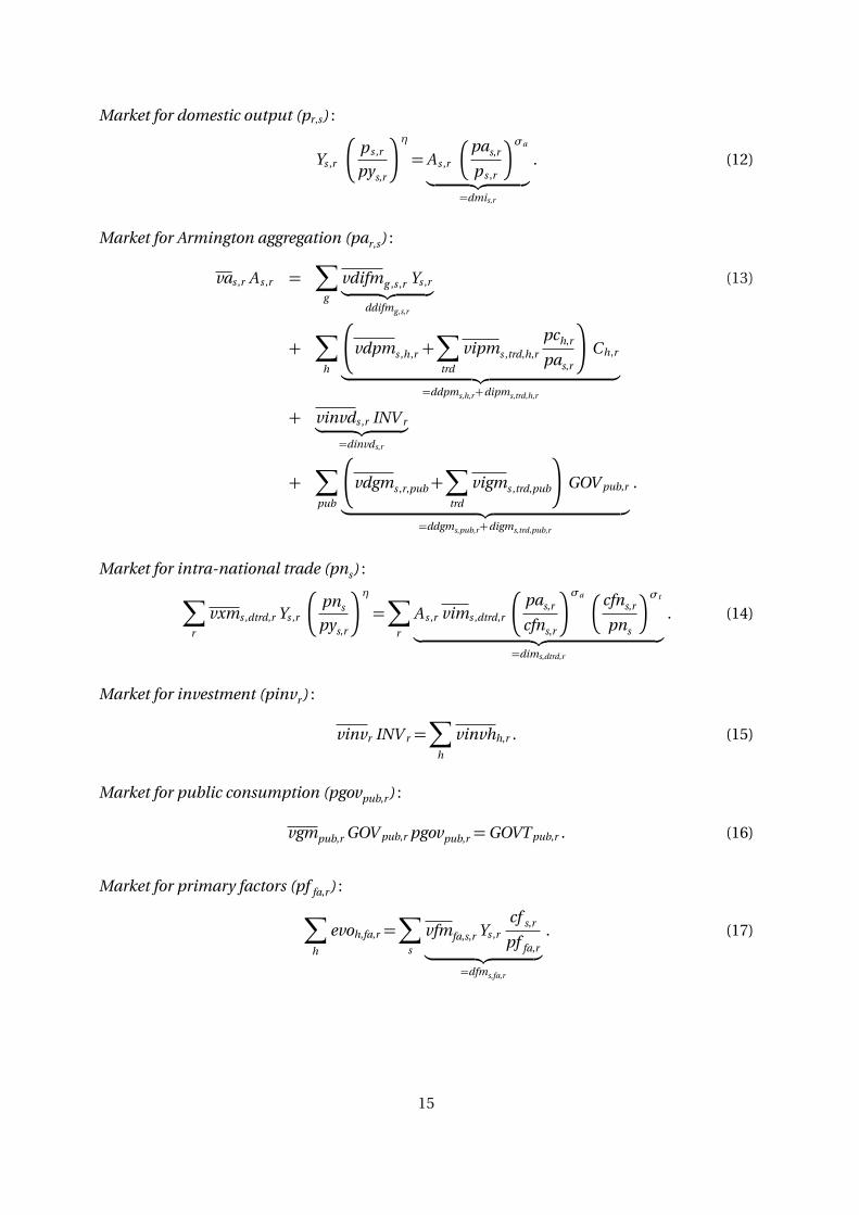
Market for domestic output (pr,s) :
Ys ,r
�ps ,r
pys,r
�η= As ,r
�pas,r
ps ,r
�σa
︸ ︷︷ ︸=dmis,r
. (12)
Market for Armington aggregation (par,s) :
vas ,r As ,r =∑
g
vdifmg ,s ,r Ys ,r︸ ︷︷ ︸ddifmg,s,r
(13)
+∑
h
vdpms ,h,r +
∑
trd
vipms ,trd,h,r
pch,r
pas,r
!Ch,r
︸ ︷︷ ︸=ddpms,h,r+dipms,trd,h,r
+ vinvds ,r INV r︸ ︷︷ ︸=dinvds,r
+∑
pub
vdgms ,r,pub+
∑
trd
vigms ,trd,pub
!GOV pub,r
︸ ︷︷ ︸=ddgms,pub,r+digms,trd,pub,r
.
Market for intra-national trade (pns) :
∑
r
vxms ,dtrd,r Ys ,r
�pns
pys,r
�η=∑
r
As ,r vims ,dtrd,r
�pas,r
cfns,r
�σa �cfns,r
pns
�σt
︸ ︷︷ ︸=dims,dtrd,r
. (14)
Market for investment (pinvr) :
vinvr INV r =∑
h
vinvhh,r . (15)
Market for public consumption (pgovpub,r) :
vgmpub,r GOV pub,r pgovpub,r =GOVT pub,r . (16)
Market for primary factors (pf fa,r) :
∑
h
evoh,fa,r =∑
s
vfmfa,s,r Ys ,r
cf s,r
pf fa,r︸ ︷︷ ︸=dfms,fa,r
. (17)
15

Market for foreign exchange (pfx) :
∑
r
∑
h
incadjh,r +∑
pub,r
vgmpub,r +∑
r
∑
s
vxms ,ftrd,r Ys ,r
�pfx
pys,r
�η(18)
=∑
r
∑
s
dfxs,r +∑
r
TAXREV r
pfx,
where
dfxs,r = As ,r vims ,,ftrd,r
�pas,r
cfns,r
�σa �cfns,r
pfx
�σt
︸ ︷︷ ︸=dims,ftrd,r
.
Market for private consumption (pcr,h) :
vpmh,r Ch,r pch,r = rhh,r . (19)
Market for price of carbon (pcarb) :∑
r
∑
pub
carbontargetp u b ,r =∑
r
∑
s
emits ,r Ys ,r , . (20)
Market for business taxes (ptax) :∑
s
vfmbtax,s,r =∑
s
vfmbtax,s,r Ys ,r . (21)
4.2.3 Income definitions
Private income (RHh,r) :
RHh,r =∑
fa
pf fa,r evoh,fa,r +pfx incadjh,r +pinvr (−vinvhh,r) . (22)
Public income (GOVT pub,r) :
GOVT pub,r = pfx vgmpub,r +pcarb carbontargetr,pub . (23)
Income of tax revenue agent (TAXREV r) :
TAXREV r = ptaxr
∑
s
vfmbtax,s,r . (24)
This completes the sets of equations that describe the equilibrium conditions. The gen-
eral equilibrium is defined by equations (7)-(24).
16

4.3 An Illustrative Counterfactual Experiment
In this section we calculate the economic costs of reducing the amount of emission permits
in the economy. We assume that emission permits are issued by the federal government
agent in each region. For simplicity, we assume that baseline emission by sector and region
are given by: emitr,s = 0.0001Yr,s. Emission permits can be traded economywide. In the
initial equilibrium, emission permits are equal to total emissions commanding a price for
carbon that equals zero.
Now consider the situation in which emission permits in each region are cut by x %. In
general, fewer emission permits drive up the price for carbon which in turn increases costs
of production. Overall, this causes national and regional output, and welfare, measured as
the change in Hicksian equivalent variation, to decrease . The virtue of carrying out this
analysis in an AGE model which is calibrated on IMPLAN data, however, lies in the capability
of disentangling economic costs by region and household type —as shown in Table 5.
TABLE 5: ECONOMIC IMPACTS OF A REDUCTION IN EMISSION PERMITS
Reduction in benchm. emission permits 2 % 4 % 6 % 8 %
Change in national output (in %) 0.30 1.05 -2.10 -6.38
Change in output by region (in %)
California 1.13 2.95 0.22 -4.03
Eastern and southern states 0.37 1.25 -1.94 -6.42
Great Lakes states 0.07 0.44 -2.43 -6.06
Plain states -0.25 -0.22 -3.77 -8.19
Western states (excluding CA) 0.15 0.91 -2.33 -6.58
Change in welfare by household (in %)
(results shown only for California)
CA.hhl -1.75 -3.97 -4.93 -5.32
CA.hh5 -1.58 -3.55 -8.28 -14.17
CA.hh10 -2.10 -4.63 -13.56 -25.20
CA.hh15 -3.43 -7.48 -19.43 -34.75
CA.hh20 -1.12 -2.45 -14.62 -31.41
CA.hh30 -1.85 -3.95 -22.46 -48.07
CA.hh40 -1.73 -3.71 -20.42 -43.65
CA.hh50 -1.59 -3.36 -22.64 -49.63
CA.hh70 -2.25 -4.76 -27.18 -58.40
17

5 Practicalities
This section describes the usage of the IMPLANinGAMS package which can be downloaded
at www.mpsge.org. The package is distributed as a zip file IMPLAN2006inGAMS.zip contain-
ing the directory structure and GAMS programs which unzips into a new directory.
5.1 System requirements
You will need to have the following:
• A recent GAMS system
• The PATH solver (installed GAMS subsystems)
• MPSGE subsystem
• Make sure you have the following files in the inclib subdirectory of your GAMS system:
domain.gms and unzip.gms. If not download www.mpsge.org/inclib/inclib.pck into
your GAMS system directory, and run gamsinst.
5.2 Getting started
GAMS source code for dataset and model management, and some template applications are
provided with the distribution directory. The package is designed to operate with a complete
national package, consisting of social accounting matricies for each of the 50 states. The
IMPLAN datafiles are not included in the tools archive. They are not distributed freely and
may be obtained from Minnesota IMPLAN Group (see www.implan.com). Here are the steps
involved in installing IMPLAN2006inGAMS:
1. Create an empty root directory named, say, IMPLAN2006inGAMS.
2. Unzip IMPLAN2006inGAMS.zip in the root directory. The root directory should have
the following subdirectories:
• build This directory contains a number of GAMS programs for reading IMPLAN
datafiles, and for filtering, balancing and aggregation of the dataset.
18

• data This directory intends to hold all data (except for the original IMPLAN data
files) in the GAMS Data eXchange (GDX) format. A number of subdirectories are
created during different stages of dataset management process to hold temporary
and final datasets.
• defines This directory contains set and mapping files which define model ag-
gregation with respect to regions, sectors, factors of production and institutions.
When aggregating a dataset, a .set file defines target sets and a .map file defines
the mapping from source to target sets.
• implandata The source IMPLAN data files have to be placed in this directory.
These can be individually zipped or flat .gms files. To be compatible with the
programs provided here, the IMPLAN data files should be named in the following
way: st%year%-%state%.* , where %year% stands for the last two digits of the
base year (e.g., “06” if 2006) and %state% stands for the standard two-character
abbreviation for states. We have appended the year of the IMPLAN source data in
order to permit comparison of model results across alternative base year datasets.
• listings This directory holds all listing .lst files that are generated during the
data management process.
• models This directory contains model source code and a few template applica-
tions.
3. Place the source state data files in the implandata directory and run build.bat.
4. Solve the sample models. The steps involved in testing the installation are in the model
subdirectory. See run.bat.
5.3 Directory Contents
Here is an overview of the files provided in the IMPLAN2006inGAMS distribution:
ROOT DIRECTORY
• build.bat Master batch file controlling the conversion of IMPLAN state-level data files
into GAMS-compatible data files. This program calls readstate.bat and merge.gms
19

• readstate.bat Batch file called by build.bat to read single state files and translate
data into GTAP-style name space. In its default operation, this program callsreadall.
gms and trnsl8.gms. Optionally, the model implan_acc.gms may be run to verify
the accounting identities implicit in the IMPLAN dataset.
• run.bat Batch file to run aggregation routine, balance domestic trade flows and verify
benchmark consistency with a template model. In its default operation, this program
calls aggregation.gms, tradeadj.gms and soe_mcp.
BUILD
• readall.gms Reads a single IMPLAN state data file and stores the data in a .gdx file. In
its default operation, this program diagonalizes IMPLAN data by converting the pro-
duction structure into a commodity rather than industry basis to produce a more com-
pact and numerically stable GE model. This feature can be deactivated by setting . In
addition, this program uses the GAMS routine domain.gms for efficient domain ex-
traction.
• trnsl8.gms The purpose of this program is (i) to translate the IMPLAN data into GTAP-
style data structures8 and (ii) to filter the data and recalibrate the resulting dataset. The
filter tolerance can be set by the parameter tol.
• merge.gms Merges single state data files into one file.
• aggregation.gms Aggregates an IMPLAN dataset.
• tradeadj.gms Performs adjustments of trade flows so that intra-state exports and im-
ports balance.
MODELS
• implan_acc.gms A static state-level model that serves to illustrate the accounting iden-
tities implicit in the IMPLAN dataset.
• soe_mcp.gms A prototype SOE regional US model to verify benchmark consistency.
This version of the model is formulated in GAMS/MCP.
8 Whenever possible, parameters holding benchmark data are chosen in accordance with the GTAP namespace as in Paltsev and Rutherford [2000].
20

• soe_mge.gms A prototype SOE regional US model to verify benchmark consistency.
This version of the model is formulated in GAMS/MPSGE.
5.4 Constructed data files
Here is an overview of the constructed data files:
• data\noaggr\merged.gdx Generated by merge.gms. Contains the national dataset
consisting of all the state data files. This files holds data that has not been aggregated,
i.e. contains individual data for all states, sectors, factors of production and institu-
tions.
• data\%target%\%target%.gdx Generated by aggregation.gms. Contains a national
aggregated dataset according to a mapping target. Domestic trade flows are not bal-
anced.
• data\%target%\%target%_dtrdbal.gdx Generated by tradeadj.gms. Contains a na-
tional aggregated dataset in which domestic trade flows have been balanced.
5.5 Aggregation
The GAMS routines provided here are designed to permit flexibility with respect to the aggre-
gation of regions, industries, factors of production and institutions. This is desirable because
(i) it allows the modeler to easily generate a dataset that is suitable for his specific research
question and (ii) careful model development typically requires to work with smaller datasets
which facilitate debugging.
Aggregation of a dataset involves the following steps:
1. Target sets and mappings have to defined in .set and .map files, respectively. Figure
7 provides an example of a .set file. Figure 8 displays a sample .map file defining
regional and sectoral aggregation. Both files have to be named identically.
2. These files have to be placed in the defines subdirectory.
3. To invoke the defined sets and mappings, specify the target in the batch file run.bat
using the name of the .set and .map file.
4. Run run.bat to aggregate the dataset (and to balanced domestic trade flows and to
verify benchmark consistency).
21

FIGURE 7: A SAMPLE .set FILE
SET reg Aggregate regions /us /;
SET S Aggregated SAM accounts /
* 5 sectors + 5 energy
SRV ServicesTRN TransportationMAN Manufactured and Processed GoodsEIS Energy Intensive SectorAGR AgricultureGAS Natural Gas DistributionCOL Coal -- SIC 12CRU Natural Gas and Crude -- SIC 13ELE Electric generation -- SIC 49OIL Refined Petroleum -- SIC 29/;
FIGURE 8: A SAMPLE .map FILE
SET mapr(*,*) Mapping from aggregate regions to states/
US.(AK,AL,AR,AZ,CA,CO,CT,DC,DE,FL,GA,HI,IA,ID,IL,IN,KS,KY,LA,MA,MD,ME,MI,MN,MO,MS,MT,NC,ND,NE,NH,NJ,NM,NV,NY,OH,OK,OR,PA,RI,SC,SD,TN,TX,UT,VA,VT,WA,WI,WV,WY) /;
SET maps(*,*) Mapping from GTAP sectors to IMPLAN 509 /
OIL.( ! Petroleum, coal products142 ! Petroleum refineries (324110:32411)143 ! Asphalt paving mixture and block manufacturing (324121:324121)144 ! Asphalt shingle and coating materials manufacturing (324122:324122)145 ! Petroleum lubricating oil and grease manufacturing (324191:324191)146 ! All other petroleum and coal products manufacturing (324199:324199)),CRU.( ! Crude oil and natural gas19 ! Oil and gas extraction (211000:211)...
22

5.6 Filtering of Small Values
The IMPLAN source data presents substantial challenges for calibrated models processed us-
ing direct solution methods (e.g., PATH, CONOPT or MINOS). Filtering is important because
the presence of large numbers of small coefficients in the source data can cause numerical
problems. These coefficients portray economic flows which are a negligible share of overall
economic activity, yet they impose a significant computational burden during matrix factor-
ization.
IMPLANinGAMS includes a piece of GAMS code (contained in trnsl8.gms) which re-
moves small values and recalibrates the resulting dataset. An input to this program, the
parameter tol, determines the filter tolerance. Values of TOL would normally range from
1e-5 to 0.01. Smaller values of tol retain a larger number of small coefficients in the filtered
dataset.
Rounding to zero depends on relative tolerances as is shown here:
* Drop sectors which have a neglible share of GDP:
zerotol(stol) = gdp*tol(stol)/10;
output(s,mkt)$(abs(output(s,mkt)) < zerotol(stol)) = 0;
* Drop inputs to production which are a negligible share of cost:
use(g,t,s)$(use(g,t,s) < tol(stol)*sum(mkt,output(g,mkt))) = 0;
iuse(g,t,i)$(iuse(g,t,i) < tol(stol)*sum(mkt,output(g,mkt))) = 0;
fd(f,t,s)$(fd(f,t,s) < tol(stol)*sum(mkt,output(s,mkt))) = 0;
simport(trd,t,s)$(abs(simport(trd,t,s)) < tol(stol)*sum(mkt,output(s,mkt))) = 0;
* Drop institutional output which is neglibly small relative to
* sectoral output:
imake(i,t,g)$(abs(imake(i,t,g)) < tol(stol)*output(g,"dmkt")) = 0;
* Drop factor endowments which are small relative to total supply:
fs(i,t,f)$(abs(fs(i,t,f)) < tol(stol)*sum((tt,ff),fs(i,tt,ff))) = 0;
fexprt(f,t,trd)$(abs(fexprt(f,t,trd)) < tol(stol)*sum((i,tt),fs(i,tt,f))) = 0;
fimprt(trd,t,f)$(abs(fimprt(trd,t,f)) < tol(stol)*sum((i,tt),fs(i,tt,f))) = 0;
23

-100%
-80%
-60%
-40%
-20%
0%
0.01 0.001 0.0005 0.0001 1e-5
filter tolerance
chan
ge in
dat
aset
non
zero
s
FIGURE 9: OVERALL IMPLAN FILTERING IMPACTS
Filtering makes a IMPLAN database smaller, as illustrated in the following Figure 9. As
indicated, filtering reduces the size of a IMPLAN database by somewhere between 30% and
90%, depending on the filtering tolerance. The filtering procedure has differential impacts
on various sub-matrices of the database. The largest proportional reduction in parameter
density occurs in the use and simport (sectoral imports) matrices. There are also substantial
reductions in the density of output and fimport (factor imports) arrays, as is indicated by
Figure 10. Lastly, Figure 11 reveals that most of the reduction in nonzeros results from the
elimination of small intermediate inputs and sectoral imports.
We believe that researchers will have their own opinions about how to select parameter
values that should be rounded to zero. The discussion presented in this section intends to
emphasize the more general point that the choice of filter tolerance does have a significant
impact on the dataset development process.
24

-100%
-80%
-60%
-40%
-20%
0%
filter tolerance
chan
ge in
com
pone
nt n
onze
ro iuse output use fd simport imake fs fimport
0.01 0.001 0.0005 0.0001 1e-5
FIGURE 10: COMPONENT FILTERING RESULTS
0%
10%
20%
30%
40%
50%
60%
70%
chan
ge in
dat
aset
non
zero
s
filter tolerance
iuse output use fd simport imake fs fimport
0.01 0.001 0.0005 0.0001 1e-5
FIGURE 11: COMPONENT CONTRIBUTIONS
25

References
MATHIESEN, L. (1985): “Computation of economic equilibria by a sequence of linear complementarity
problems,” Mathematical Programming Study, 23, 144–162.
MINNESOTA IMPLAN GROUP (2004): “User-Analysis-Data Guide,” 3rd edition, available at:
www.implan.com.
PALTSEV, S. V., AND T. F. RUTHERFORD (2000): “GTAPinGAMS and GTAP-EG: Global Datasets for Eco-
nomic Research and Illustrative Models,” Working Paper, Department of Economics, University of
Colorado.
RUTHERFORD, T. F. (1995): “Extension of GAMS for complementarity problems arising in applied eco-
nomics,” Journal of Economic Dynamics and Control, 19(8), 1299–1324.
(1999): “Applied general equilibrium modeling with MPSGE as a GAMS subsystem: an
overview of the modeling framework and syntax,” Computational Economics, 14, 1–46.
26

A GAMS/MPSGE Code: IMPLAN State-Level Accounting Model
$title Simple Static State-Level Model
* This model "implan_acc.gms" serves to illustrate the accounting
* identities implicit in the IMPLAN dataset.
$if not set ds $set ds ak
$batinclude statedata
$ontext
$model:soe
$sectors:
y(s)$vom(s) ! Sectoral production
m(g,trd)$vim(g,trd) ! Commodity imports
cd(h)$vpm(h) ! Household demand
gd(pub)$vgm(pub) ! Government demand
id ! Investment demand
$commodities:
py(g)$vom(g) ! Domestic output
pm(g,trd)$vim(g,trd) ! Import price
pc(h)$vpm(h) ! Household demand
pi ! Investment
pg(pub) ! Public demand
pr(f) ! Factor supplies
prf ! Corporate profits
pfx ! Foreign exchange
$consumers:
rh(h) ! Representative households
rg(pub) ! Representative public institutions
firms ! Representative firms
$auxiliary:
x(s)$vx(s) ! Sectoral exports
fx ! Foreign exchange earnings
27
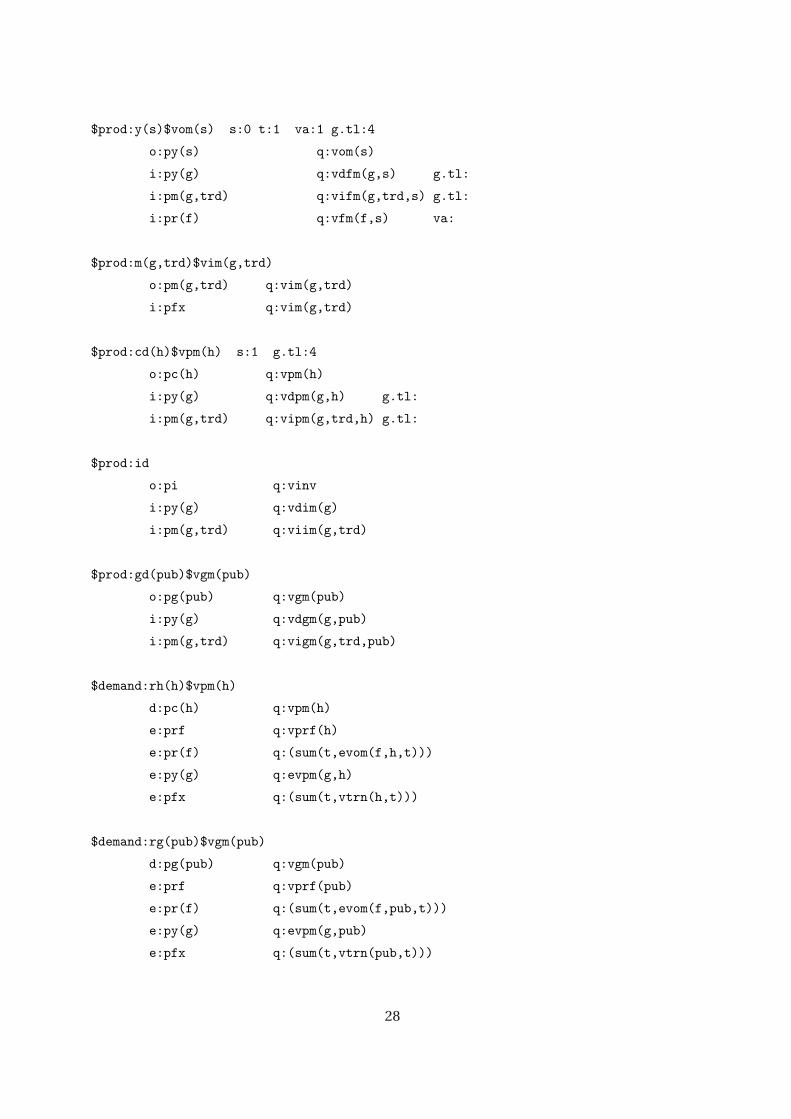
$prod:y(s)$vom(s) s:0 t:1 va:1 g.tl:4
o:py(s) q:vom(s)
i:py(g) q:vdfm(g,s) g.tl:
i:pm(g,trd) q:vifm(g,trd,s) g.tl:
i:pr(f) q:vfm(f,s) va:
$prod:m(g,trd)$vim(g,trd)
o:pm(g,trd) q:vim(g,trd)
i:pfx q:vim(g,trd)
$prod:cd(h)$vpm(h) s:1 g.tl:4
o:pc(h) q:vpm(h)
i:py(g) q:vdpm(g,h) g.tl:
i:pm(g,trd) q:vipm(g,trd,h) g.tl:
$prod:id
o:pi q:vinv
i:py(g) q:vdim(g)
i:pm(g,trd) q:viim(g,trd)
$prod:gd(pub)$vgm(pub)
o:pg(pub) q:vgm(pub)
i:py(g) q:vdgm(g,pub)
i:pm(g,trd) q:vigm(g,trd,pub)
$demand:rh(h)$vpm(h)
d:pc(h) q:vpm(h)
e:prf q:vprf(h)
e:pr(f) q:(sum(t,evom(f,h,t)))
e:py(g) q:evpm(g,h)
e:pfx q:(sum(t,vtrn(h,t)))
$demand:rg(pub)$vgm(pub)
d:pg(pub) q:vgm(pub)
e:prf q:vprf(pub)
e:pr(f) q:(sum(t,evom(f,pub,t)))
e:py(g) q:evpm(g,pub)
e:pfx q:(sum(t,vtrn(pub,t)))
28

$demand:firms
d:prf q:(sum(i,vprf(i)))
e:pi q:(-vinv)
e:pr(f) q:(sum((corp,t),evom(f,corp,t)))
e:py(g) q:(sum(corp,evpm(g,corp)))
e:pfx q:(sum((corp,t),vtrn(corp,t)))
e:py(s)$vx(s) q:(-1) r:x(s)
e:pfx q:1 r:fx
$constraint:x(s)$vx(s)
x(s) =e= sum(trd, vxm(s,trd) * (pfx/py(s))**5);
$constraint:fx
fx * pfx =e= sum(s$vx(s), py(s)*x(s));
$offtext
$sysinclude mpsgeset soe
x.l(s) = vx(s);
fx.l = sum(s, vx(s));
soe.workspace = 25;
soe.iterlim = 0;
$include soe.gen
solve soe using mcp;
29

B GAMS/MCP Code: Prototype US Regional Model
$title Simple Static Small Open Economy Model with Intra-national Trade
$if not set target $set target gtap
* Read the dataset using the utility program:
$batinclude models\regionaldata
* Define set for primary factor of production and taxes:
SET fa(f) /empl,prop,othp/
ft(f) /btax/;
ALIAS (fa,ffa);
* Install parameters for model specification:
PARAMETER
vdifm(r,g,s) Total intermediate demand
evo(r,i,f) Factor endowment by institution
va(r,s) Armington supply including imports
vn(g) Intra-national trade
vinvd(r,g) Investment demand by commodity
vinvh(r,h) Investment demand by household
incadj(r,h) Base year net transfer
tc(r,s) Carbon tax rate
carbontarget Carbon emissions target
emit(r,s) Base year emissions;
vdifm(r,g,s) = vdfm(r,g,s) + sum(trd, vifm(r,g,trd,s));
evo(r,i,f) = sum(t, evom(r,f,i,t));
va(r,s) = sum(trd,vim(r,s,trd)) + vdmi(r,s);
vn(g) = sum(r, vxm(r,g,"dtrd"))+eps;
* Impute investment demand to households:
vinvd(r,g) = va(r,g) - (sum(h,vdpm(r,g,h))+sum((trd,h),vipm(r,g,trd,h)))
- (sum(pub,vdgm(r,g,pub))+sum((trd,pub),vigm(r,g,trd,pub)))
30

- sum(s, vdifm(r,g,s));
* Impute wage payments, capital payments:
vfm(r,"empl",s) = max(vdmi(r,s)+sum(trd,vxm(r,s,trd))
- (vfm(r,"prop",s) + vfm(r,"othp",s)) - vfm(r,"btax",s)
- sum(g, vdifm(r,g,s)), 0);
vfm(r,"prop",s) = max(vdmi(r,s)+sum(trd,vxm(r,s,trd))
- (vfm(r,"empl",s) + vfm(r,"othp",s)) - vfm(r,"btax",s)
- sum(g, vdifm(r,g,s)), 0);
vfm(r,"othp",s) = max(vdmi(r,s)+sum(trd,vxm(r,s,trd))
- (vfm(r,"empl",s) + vfm(r,"prop",s)) - vfm(r,"btax",s)
- sum(g, vdifm(r,g,s)), 0);
vfm(r,"btax",s) = vdmi(r,s)+sum(trd,vxm(r,s,trd))
- (vfm(r,"prop",s) + vfm(r,"othp",s)) - vfm(r,"empl",s)
- sum(g, vdifm(r,g,s));
* Scale labor endowments to match imputed wage payments:
evo(r,h,"empl") = evo(r,h,"empl")/sum(hh, evo(r,hh,"empl"))
* sum(s, vfm(r,"empl",s));
evo(r,h,"prop") = evo(r,h,"prop")/sum(hh,evo(r,hh,"prop"))
* sum(s, vfm(r,"prop",s));
evo(r,h,"othp") = evo(r,h,"othp")/sum(hh,evo(r,hh,"othp"))
* sum(s, vfm(r,"othp",s));
* Impute aggregate investment and investment demand by household:
vinv(r) = sum(g, vinvd(r,g));
vinvh(r,h)$sum(hh, max(0, sum(t,trnsfer(r,"inv",t,hh) - trnsfer(r,hh,t,"inv"))))
= max(0, sum(t, trnsfer(r,"inv",t,h) - trnsfer(r,h,t,"inv"))) /
sum(hh, max(0, sum(t, trnsfer(r,"inv",t,hh)
- trnsfer(r,hh,t,"inv"))))* vinv(r);
* Adjust household income:
incadj(r,h) = sum(g,vdpm(r,g,h)+sum(trd,vipm(r,g,trd,h)))
+ vinvh(r,h) - sum(f,evo(r,h,f));
* Base year emissions:
31

emit(r,s) = 1e-4 * (vdmi(r,s) + sum(trd,vxm(r,s,trd)));
carbontarget(r) = sum(s,emit(r,s));
* Define elasticity parameters:
PARAMETER
eta ES of transformation /2/
es_a EOS bw domestic and traded goods /4/
es_t EOS bw domestically and foreign traded goods /8/;
* Define value share parameters to simplify algebra:
PARAMETER
thetai(r,s) Value share of intermediate input
thetaf(r,s) Value added share of sectoral output
thetae(r,s) Value share of emmissions
thetat(r,s) Value share of business taxes;
thetai(r,s)$vdmi(r,s) = sum(g,vdifm(r,g,s))/(vdmi(r,s)+sum(trd,vxm(r,s,trd)));
thetaf(r,s)$vdmi(r,s) = sum(fa,vfm(r,fa,s)/(vdmi(r,s)+sum(trd,vxm(r,s,trd))));
thetae(r,s)$vdmi(r,s) = emit(r,s)/(vdmi(r,s)+sum(trd,vxm(r,s,trd)));
thetat(r,s)$vdmi(r,s) = vfm(r,"btax",s)/(vdmi(r,s)+sum(trd,vxm(r,s,trd)));
*--------------------------------------------------------------------------
* Formulate a stylized SOE US regional model in GAMS/MCP based on
* hese statistics and verify that the resulting data represents
* an equilibrium:
POSITIVE VARIABLES
y(r,s) Sectoral production
a(r,s) Armington aggregation
c(r,h) Consumption by household
gov(r,pub) Public output
inv(r) Investment
p(r,s) Sectoral output prices
pa(r,s) Armington aggregate prices
pc(r,h) Consumption by household
pn(s) Intra-national trade price
32

pinv(r) New investment
pgov(r,pub) Public output
pf(r,fa) Factor prices
pfx Foreign exchange
pcarb Tradable CO2 emission permit price
ptax(r) Business taxes
rh(r,h) Representative households
govt(r,pub) Government (different levels)
taxrev Tax revenue agent
target Rationing variable for emission permits
cf(r,s) User cost index for primary factors
ca(r,s) User cost index for Armington inputs
cfn(r,g) User cost index for domestic and imported inputs
dfm(fa,r,s) Sectoral demand for primary factors
dfx(r,g) Armington demand for foreign exchange
dfn(r,g) Armington demand for domestic trade
da(r,s,g) Sectoral demand for Armington good
dad(r,g) Armington demand for domestic output
py(r,s) Price for sectoral output;
EQUATIONS
prf_y(r,s) Sectoral production
prf_a(r,s) Armington aggregation
prf_c(r,h) Consumption by household
prf_gov(r,pub) Public output
prf_inv(r) Investment
mkt_p(r,s) Sectoral output prices
mkt_pa(r,s) Armington aggregate prices
mkt_pc(r,h) Consumption by household
mkt_pn(s) Intra-national trade price
mkt_pinv(r) New investment
mkt_pgov(r,pub) Public output
mkt_pf(r,fa) Factor prices
mkt_pfx Foreign exchange
mkt_pcarb Tradable CO2 emission permit price
mkt_ptax(r) Business taxes
33

inc_rh(r,h) Representative households
inc_govt(r,pub) Government (different levels)
inc_taxrev(r) Tax revenue agent
eq_cf(r,s)
eq_ca(r,s) User cost index for Armington inputs
eq_cfn(r,g) User cost index for domestic and imported inputs
eq_dfm(fa,r,s) Sectoral demand for primary factors
eq_dfx(r,g) Armington demand for foreign exchange
eq_dfn(r,g) Armington demand for domestic trade
eq_da(r,s,g) Sectoral demand for Armington good
eq_dad(r,g) Armington demand for domestic output
eq_py(r,s) Price for sectoral output;
* Equation definitions to simplify algebra:
eq_cf(r,s)$(sum(fa,vfm(r,fa,s))).. cf(r,s) =e= prod(fa, pf(r,fa)**(vfm(r,fa,s)
/sum(ffa,vfm(r,ffa,s))));
eq_ca(r,s)$(sum(g, vdifm(r,g,s))).. ca(r,s) =e=
sum(g, vdifm(r,g,s)/sum(gg,vdifm(r,gg,s)) * PA(r,g));
eq_cfn(r,g)$(sum(trd,vim(r,g,trd))).. cfn(r,g) =e=
(vim(r,g,"ftrd")/sum(trd,vim(r,g,trd))*PFX**(1-es_t)
+ vim(r,g,"dtrd")/sum(trd,vim(r,g,trd))
*PN(g)**(1-es_t))**(1/(1-es_t));
eq_dfm(fa,r,s).. dfm(fa,r,s) =e= vfm(r,fa,s)*Y(r,s)*cf(r,s)/pf(r,fa);
eq_dfx(r,g).. dfx(r,g) =e= A(r,g) * vim(r,g,"ftrd")
*(PA(r,g)/cfn(r,g))**es_a * (cfn(r,g)/PFX)**es_t;
eq_dfn(r,g).. dfn(r,g) =e= A(r,g) * vim(r,g,"dtrd")
*(cfn(r,g)/PA(r,g))**(-es_a) * (cfn(r,g)/PN(g))**es_t;
eq_da(r,s,g).. da(r,s,g) =e= vdifm(r,g,s)*Y(r,s);
eq_dad(r,g).. dad(r,g) =e= vdmi(r,g)*A(r,g)*(PA(r,g)/P(r,g))**es_a;
34
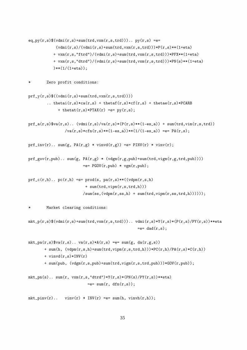
eq_py(r,s)$(vdmi(r,s)+sum(trd,vxm(r,s,trd))).. py(r,s) =e=
(vdmi(r,s)/(vdmi(r,s)+sum(trd,vxm(r,s,trd)))*P(r,s)**(1+eta)
+ vxm(r,s,"ftrd")/(vdmi(r,s)+sum(trd,vxm(r,s,trd)))*PFX**(1+eta)
+ vxm(r,s,"dtrd")/(vdmi(r,s)+sum(trd,vxm(r,s,trd)))*PN(s)**(1+eta)
)**(1/(1+eta));
* Zero profit conditions:
prf_y(r,s)$((vdmi(r,s)+sum(trd,vxm(r,s,trd))))
.. thetai(r,s)*ca(r,s) + thetaf(r,s)*cf(r,s) + thetae(r,s)*PCARB
+ thetat(r,s)*PTAX(r) =e= py(r,s);
prf_a(r,s)$va(r,s).. (vdmi(r,s)/va(r,s)*(P(r,s)**(1-es_a)) + sum(trd,vim(r,s,trd))
/va(r,s)*cfn(r,s)**(1-es_a))**(1/(1-es_a)) =e= PA(r,s);
prf_inv(r).. sum(g, PA(r,g) * vinvd(r,g)) =e= PINV(r) * vinv(r);
prf_gov(r,pub).. sum(g, PA(r,g) * (vdgm(r,g,pub)+sum(trd,vigm(r,g,trd,pub))))
=e= PGOV(r,pub) * vgm(r,pub);
prf_c(r,h).. pc(r,h) =e= prod(s, pa(r,s)**((vdpm(r,s,h)
+ sum(trd,vipm(r,s,trd,h)))
/sum(ss,(vdpm(r,ss,h) + sum(trd,vipm(r,ss,trd,h))))));
* Market clearing conditions:
mkt_p(r,s)$(vdmi(r,s)+sum(trd,vxm(r,s,trd))).. vdmi(r,s)*Y(r,s)*(P(r,s)/PY(r,s))**eta
=e= dad(r,s);
mkt_pa(r,s)$va(r,s).. va(r,s)*A(r,s) =e= sum(g, da(r,g,s))
+ sum(h, (vdpm(r,s,h)+sum(trd,vipm(r,s,trd,h)))*PC(r,h)/PA(r,s)*C(r,h))
+ vinvd(r,s)*INV(r)
+ sum(pub, (vdgm(r,s,pub)+sum(trd,vigm(r,s,trd,pub)))*GOV(r,pub));
mkt_pn(s).. sum(r, vxm(r,s,"dtrd")*Y(r,s)*(PN(s)/PY(r,s))**eta)
=e= sum(r, dfn(r,s));
mkt_pinv(r).. vinv(r) * INV(r) =e= sum(h, vinvh(r,h));
35

mkt_pgov(r,pub).. vgm(r,pub) * GOV(r,pub) * PGOV(r,pub) =e= GOVT(r,pub);
mkt_pf(r,fa).. sum(h,evo(r,h,fa)) =e= sum(s, dfm(fa,r,s));
mkt_pfx.. sum((r,h), incadj(r,h)) + sum((r,pub), vgm(r,pub))
+ sum((r,s), vxm(r,s,"ftrd")*Y(r,s)*(PFX/PY(r,s))**eta)
=e= sum((r,s), dfx(r,s)) + sum(r, taxrev(r)/PFX);
mkt_pc(r,h).. vpm(r,h) * C(r,h) * PC(r,h) =e= RH(r,h);
mkt_pcarb.. sum((r,pub),carbontarget(r)$(ord(pub) eq 1)) =e= sum((r,s), emit(r,s) * Y(r,s));
mkt_ptax(r).. sum(s,vfm(r,"btax",s)) =e= sum(s, vfm(r,"btax",s) * Y(r,s));
* Income definitions:
inc_rh(r,h).. RH(r,h) =e= sum(fa, pf(r,fa)*evo(r,h,fa))
+ pfx*incadj(r,h) + pinv(r)*(-vinvh(r,h));
inc_govt(r,pub).. GOVT(r,pub) =e= pfx*vgm(r,pub) + pcarb*carbontarget(r)$(ord(pub) eq 1);
inc_taxrev(r).. TAXREV(r) =e= ptax(r) * sum(s, vfm(r,"btax",s));
* Define model and match equations and variables:
model soe_mcp /prf_y.y,prf_a.a,prf_c.c,prf_gov.gov,prf_inv.inv,mkt_p.p,
mkt_pa.pa,mkt_pc.pc,mkt_pn.pn,mkt_pinv.pinv,mkt_pgov.pgov,
mkt_pf.pf,mkt_pfx.pfx,mkt_pcarb.pcarb,mkt_ptax.ptax,inc_rh.rh,
inc_govt.govt,inc_taxrev.taxrev,eq_cf.cf,
eq_ca.ca,eq_cfn.cfn,eq_dfm.dfm,eq_dfx.dfx,eq_dfn.dfn,eq_da.da,
eq_dad.dad,eq_py.py/;
* Assign default values:
y.l(r,s)=1;a.l(r,s)=1;c.l(r,h)=1;gov.l(r,pub)=1;inv.l(r)=1;p.l(r,s)=1;
pa.l(r,s)=1;pc.l(r,h)=1;pn.l(s)=1;pinv.l(r)=1;pgov.l(r,pub)=1;pf.l(r,fa)=1;
pfx.l=1;pcarb.l=0;ptax.l(r)=1;rh.l(r,h)=vpm(r,h);govt.l(r,pub)=vgm(r,pub);
cf.l(r,s)=1;ca.l(r,s)=1;cfn.l(r,g)=1;dfm.l(fa,r,s)=vfm(r,fa,s);
dfx.l(r,g)=vim(r,g,"ftrd");dfn.l(r,g)=vim(r,g,"dtrd");da.l(r,s,g)=vdifm(r,g,s);
dad.l(r,g)=vdmi(r,g);py.l(r,s)=1;taxrev.l(r)=sum(s, vfm(r,"btax",s));
36

* Fix variables which should not be in the model:
PN.fx(s)$(vn(s)=0) =1;
* Choose a numeraire:
PFX.fx =1;
* Verify benchmark consistency:
soe_mcp.iterlim = 0;
solve soe_mcp using mcp;
37

C GAMS/MPSGE Code: Prototype US Regional Model
$title Simple Static Small Open Economy Model with Intra-national Trade
$if not set target $set target gtap
* Read the dataset using the utility program:
$batinclude models\regionaldata
* Define set for primary factor of production and taxes:
SET fa(f) /empl,prop,othp/
ft(f) /btax/;
* Install parameters for model specification:
PARAMETER
vdifm(r,g,s) Total intermediate demand
evo(r,i,f) Factor endowment by institution
va(r,s) Armington supply including imports
vn(g) Intra-national trade
vinvd(r,g) Investment demand by commodity
vinvh(r,h) Investment demand by household
incadj(r,h) Base year net transfer
tc(r,s) Carbon tax rate
carbontarget Carbon emissions target
emit(r,s) Base year emissions;
vdifm(r,g,s) = vdfm(r,g,s) + sum(trd, vifm(r,g,trd,s));
evo(r,i,f) = sum(t, evom(r,f,i,t));
va(r,s) = sum(trd,vim(r,s,trd)) + vdmi(r,s);
vn(g) = sum(r, vxm(r,g,"dtrd"));
* Impute investment demand to households:
vinvd(r,g) = va(r,g) - (sum(h,vdpm(r,g,h))+sum((trd,h),vipm(r,g,trd,h)))
- (sum(pub,vdgm(r,g,pub))+sum((trd,pub),vigm(r,g,trd,pub)))
- sum(s, vdifm(r,g,s));
38

* Impute wage payments, capital payments:
vfm(r,"empl",s) = max(vdmi(r,s)+sum(trd,vxm(r,s,trd))
- (vfm(r,"prop",s) + vfm(r,"othp",s)) - vfm(r,"btax",s)
- sum(g, vdifm(r,g,s)), 0);
vfm(r,"prop",s) = max(vdmi(r,s)+sum(trd,vxm(r,s,trd))
- (vfm(r,"empl",s) + vfm(r,"othp",s)) - vfm(r,"btax",s)
- sum(g, vdifm(r,g,s)), 0);
vfm(r,"othp",s) = max(vdmi(r,s)+sum(trd,vxm(r,s,trd))
- (vfm(r,"empl",s) + vfm(r,"prop",s)) - vfm(r,"btax",s)
- sum(g, vdifm(r,g,s)), 0);
vfm(r,"btax",s) = vdmi(r,s)+sum(trd,vxm(r,s,trd))
- (vfm(r,"prop",s) + vfm(r,"othp",s)) - vfm(r,"empl",s)
- sum(g, vdifm(r,g,s));
* Scale labor endowments to match imputed wage payments:
evo(r,h,"empl") = evo(r,h,"empl")/sum(hh, evo(r,hh,"empl"))
* sum(s, vfm(r,"empl",s));
evo(r,h,"prop") = evo(r,h,"prop")/sum(hh,evo(r,hh,"prop"))
* sum(s, vfm(r,"prop",s));
evo(r,h,"othp") = evo(r,h,"othp")/sum(hh,evo(r,hh,"othp"))
* sum(s, vfm(r,"othp",s));
* Impute aggregate investment and investment demand by household:
vinv(r) = sum(g, vinvd(r,g));
vinvh(r,h)$sum(hh, max(0, sum(t,trnsfer(r,"inv",t,hh) - trnsfer(r,hh,t,"inv"))))
= max(0, sum(t, trnsfer(r,"inv",t,h) - trnsfer(r,h,t,"inv"))) /
sum(hh, max(0, sum(t, trnsfer(r,"inv",t,hh)
- trnsfer(r,hh,t,"inv"))))* vinv(r);
* Adjust household income:
incadj(r,h) = sum(g,vdpm(r,g,h)+sum(trd,vipm(r,g,trd,h)))
+ vinvh(r,h) - sum(f,evo(r,h,f));
* Base year emissions:
emit(r,s) = 1e-4 * (vdmi(r,s) + sum(trd,vxm(r,s,trd)));
39

carbontarget(r) = sum(s,emit(r,s));
* Define elasticity parameters:
PARAMETER
eta ES of transformation /2/
es_a EOS bw domestic and traded goods /4/
es_t EOS bw domestically and foreign traded goods /8/;
*--------------------------------------------------------------------------
* Formulate a stylized SOE US regional model in GAMS/MPSGE based on
* hese statistics and verify that the resulting data represents
* an equilibrium:
$ontext
$model:soe
$sectors:
y(r,s)$(vdmi(r,s)+sum(trd,vxm(r,s,trd))) ! Sectoral production
a(r,s)$va(r,s) ! Armington aggregation
c(r,h) ! Consumption by household
gov(r,pub) ! Public output
inv(r) ! Investment
$commodities:
p(r,s)$(vdmi(r,s)+sum(trd,vxm(r,s,trd))) ! Sectoral output prices
pc(r,h) ! Consumption by household
pa(r,s)$va(r,s) ! Armington aggregate prices
pn(s)$vn(s) ! Intra-national trade price
pinv(r) ! New investment
pgov(r,pub) ! Public output
pf(r,fa)$(sum(s,vfm(r,fa,s))) ! Factor prices
pfx ! Foreign exchange
pcarb ! Tradable CO2 emission permit price
ptax(r)$(sum(s,vfm(r,"btax",s))) ! Business taxes
$consumers:
rh(r,h) ! Representative households
govt(r,pub) ! Government (different levels)
40

taxrev(r) ! Tax revenue agent
$prod:y(r,s)$(vdmi(r,s)+sum(trd,vxm(r,s,trd))) s:0 t:eta va:1
o:p(r,s) q:vdmi(r,s)
o:pfx q:vxm(r,s,"ftrd")
o:pn(s) q:vxm(r,s,"dtrd")
i:pa(r,g) q:vdifm(r,g,s)
i:pf(r,fa) q:vfm(r,fa,s) va:
i:pcarb q:emit(r,s)
i:ptax(r) q:vfm(r,"btax",s)
$prod:a(r,s)$va(r,s) s:es_a m:es_t
o:pa(r,s) q:va(r,s)
i:p(r,s) q:vdmi(r,s)
i:pfx q:vim(r,s,"ftrd") m:
i:pn(s) q:vim(r,s,"dtrd") m:
$prod:inv(r)
o:pinv(r) q:vinv(r)
i:pa(r,s) q:vinvd(r,s)
$prod:gov(r,pub)
o:pgov(r,pub) q:vgm(r,pub)
i:pa(r,s) q:(vdgm(r,s,pub)+sum(trd,vigm(r,s,trd,pub)))
$prod:c(r,h) s:1
o:pc(r,h) q:vpm(r,h)
i:pa(r,s) q:(vdpm(r,s,h)+sum(trd,vipm(r,s,trd,h)))
$demand:rh(r,h)
d:pc(r,h) q:vpm(r,h)
e:pf(r,fa) q:evo(r,h,fa)
e:pfx q:incadj(r,h)
e:pinv(r) q:(-vinvh(r,h))
$demand:govt(r,pub)
d:pgov(r,pub) q:vgm(r,pub)
e:pfx q:vgm(r,pub)
e:pcarb q:(carbontarget(r)$(ord(pub) eq 1))
41

$demand:taxrev(r)
d:pfx
e:ptax(r) q:(sum(s,vfm(r,"btax",s)))
$report:
v:yd(r,s) o:p(r,s) prod:y(r,s)
v:yftrd(r,s) o:pfx prod:y(r,s)
v:ydtrd(r,s) o:pn(s) prod:y(r,s)
$offtext
$sysinclude mpsgeset soe
* Choose a numeraire:
PFX.fx = 1;
soe.workspace = 40;
soe.iterlim = 1;
$include soe.gen
solve soe using mcp;
abort$(abs(soe.objval) gt 1e-8) "***Model does not calibrate***";
*-----------------------------------------------------------------------------------------
* Run a series of counterfactuals which reduce the amount of emission permits
* in the economony:
* Define report parameters:
PARAMETER rcarbt Percentage reduction of base year emission (permits)
rpcarb Price of carbon
cons Welfare change by household tpye and region
no_b Benchmark value of national output
ro_b Benchmark value of regional output
nationaloutput Change in national output (in%)
regionaloutput Change in regional output (in%);
no_b = sum((r,s),yd.l(r,s)*p.l(r,s) + yftrd.l(r,s)*pfx.l+ydtrd.l(r,s)*pn.l(s));
ro_b(r) = sum(s,yd.l(r,s)*p.l(r,s) + yftrd.l(r,s)*pfx.l+ydtrd.l(r,s)*pn.l(s));
* Define an iteration index:
42

SET z /1*4/;
* Solve a series of models (in the benchmark the price for carbon is zero,
ie the cap is not binding):
LOOP(z,
* Reduce emission permits:
carbontarget(r) = (1-0.02*ord(z))*sum(s,emit(r,s));
soe.iterlim = 10000;
$include soe.gen
solve soe using mcp;
rcarbt(z) = 100*ord(z)*0.02;
cons("CA",h,z) = 100*(c.l("CA",h)-1);
nationaloutput(z) = 100*(sum((r,s),yd.l(r,s)*p.l(r,s) + yftrd.l(r,s)
*pfx.l+ydtrd.l(r,s)*pn.l(s))/no_b-1);
regionaloutput(r,z) = 100*(sum(s,yd.l(r,s)*p.l(r,s) + yftrd.l(r,s)
*pfx.l+ydtrd.l(r,s)*pn.l(s))/ro_b(r)-1);
rpcarb(z) = pcarb.l;
);
DISPLAY rcarbt,rpcarb,cons,nationaloutput,regionaloutput;
43