To Read 1106

8/6/2019 To Read 1106

http://slidepdf.com/reader/full/to-read-1106 1/15

a r X i v : 1 1 0 6 . 2 2 1 6 v 1

[ a s t r o - p h . H E ] 1 1 J u n 2 0 1 1

A NOVEL EMISSION SPECTRUM FROM A RELATIVISTIC

ELECTRON MOVING IN A RANDOM MAGNETIC FIELD

Yuto Teraki1 and Fumio Takahara1

Department of Earth and Space Science, Graduate School of Science, Osaka University, 1-1

Machikaneyama-cho, Toyonaka, Osaka 560-0043, Japan

[email protected]

ABSTRACT

We calculate numerically the radiation spectrum from relativistic electrons

moving in small scale turbulent magnetic fields expected in high energy astro-

physical sources. Such radiation spectrum is characterized by the strength pa-

rameter a = λBe|B|/mc2, where λB is the length scale of the turbulent field.

When a is much larger than the Lorentz factor of a radiating electron γ , syn-

chrotron radiation is realized, while a ≪ 1 corresponds to the so-called jitter

radiation regime. Because for 1 < a < γ we cannot use either approximations,

we should have recourse to the Lienard-Wiechert potential to evaluate the radia-

tion spectrum, which is performed in this paper. We generate random magnetic

fields assuming Kolmogorov turbulence, inject monoenergetic electrons, solve the

equation of motion, and calculate the radiation spectrum. We perform numeri-cal calculations for several values of a with γ = 10. We obtain various types of

spectra ranging between jitter radiation and synchrotron radiation. For a ∼ 7,

the spectrum turns out to take a novel shape which has not been noticed up to

now. It is like a synchrotron spectrum in the middle energy region, but in the

low frequency region it is a broken power law and in the high frequency region

an extra power law component appears beyond the synchrotron cutoff. We give

a physical explanation of these features.

Subject headings: magnetic fields — turbulence — radiation mechanisms: gen-

eral — gamma-ray burst: general

1. Introduction

A major part of non-thermal emission from high energy astrophysical objects is almost

always characterized by the radiation from relativistic electrons moving in magnetic fields.

http://fr.arxiv.org/abs/1106.2216v1








































8/6/2019 To Read 1106


– 2 –

Usually it is interpreted in terms of the synchrotron radiation. However, synchrotron ap-

proximation is not always valid, in particular when the magnetic fields are highly turbulent.

Electrons suffer from random accelerations and do not trace a helical trajectory. In general,the radiation spectrum is characterized by the strength parameter

a = λB

e|B|mc2

, (1)

where λB is the typical scale of turbulent fields, |B| is the mean value of the turbulent

magnetic fields, e is the elementary charge, m is the mass of electron and c is the speed

of light (Reville & Kirk 2010). When a ≫ γ , where γ is the Lorentz factor of radiating

electron, the scale of turbulent fields is much larger than the Larmor radius rg ≡ γmc2/e|B|,and electrons move in an approximately uniform field, so that the synchrotron approximation

is valid. In contrast, when a≪

1, λB is much smaller than the scale rg/γ = λB/a which

corresponds to the emission of the characteristic synchrotron frequency. In this regime,

electrons move approximately straightly, and jitter approximation or the weak random field

regime of diffusive synchrotron radiation (DSR) can be applied (Medvedev 2010, Fleishman

and Urtiev 2010). For 1 a γ , no simple approximation of the radiation spectrum has

been known.

The standard model of Gamma Ray Bursts (GRB) is based on the synchrotron radia-

tion from accelerated electrons at the internal shocks. The observational spectra of prompt

emission of GRB can be well fitted by a broken power law spectrum which is called the

Band function. Around a third of GRBs show a spectrum in the low energy side harder than

the synchrotron theory predicts. To explain this, other radiation mechanisms are needed.Medvedev examined relativistic collisionless shocks in relevance to internal shocks of GRB,

and noticed the generation of small scale turbulent magnetic fields near the shock front

(Medvedev & Loeb 1999). Then he calculated analytically radiation spectrum from elec-

trons moving in small scale turbulent magnetic fields, to make a harder spectrum than the

synchrotron radiation (Medvedev 2000). However, he assumed that the strength parame-

ter a is much smaller than 1 and that turbulent field is of one-dimensional structure, which

may be over simplified in general (Fleishman 2006). Medvedev also calculated 3-dimensional

structure assuming that the turbulent field is highly anisotropic (Medvedev 2006). He con-

clude that the harder spectrum is achieved in ”head on” case, and that in ”edge on” case,the spectrum is softer than synchrotron radiation. The spectral index depends on the angle

θ between the particle velocity and shock normal with hard spectrum obtained when θ 10

(Medvedev 2009).

Recently several particle-in-cell (PIC) simulations of relativistic collisionless shocks have

been performed to study the nature of turbulent magnetic fields which are generated near

the shock front (e.g., Frederiksen et al. 2004; Kato 2005; Chang et al. 2008; Haugbolle

8/6/2019 To Read 1106


– 3 –

2010). The characteristic scale of the magnetic fields is the order of skin depth as predicted

by the analysis of Weibel instability. Then, the wavelength of turbulent magnetic field λB is

described by using a coefficient κ asλB = κ

c

ωpeΓint

, (2)

where ωpe is the plasma frequency, and Γint is the relative Lorentz factor between colliding

shells. The energy conversion fraction into the magnetic fields

εB =B2/8π

Γintnmpc2(3)

is 10−3− 0.1, where B2/8π is energy density of magnetic fields, and Γintnmpc2 is the kinetic

energy density of the shell. The Lorentz factor of electrons is similar to Γint, and that κ is

typically 10 from the result of PIC simulations, the strength parameter a can be estimatedas

a =√

2κεB1/2

mp

me

∼ O(1− 102). (4)

Thus, the assumption a ≪ 1 on which jitter radiation and DSR weak random field regime

are based is not necessarily valid when we consider the radiation from the internal shock

region of GRB.

Fleishman & Urtiev (2010) calculated the radiation spectrum for a > 1 using a statistical

method, but their treatment of the ”small scale component” is somewhat arbitrary. They

introduced the critical wavelength λcrit and called components with λ ≤ λcrit the ”small scalecomponent”, where λcrit obeys the inequality

rg ≪ λcrit ≪ rg/γ (5)

(Toptygin & Fleishman 1987). The inequality can be transformed to 1 ≪ λcrite|B|/mc2 ≪ γ ,

so that the division through λcrit may be ambiguous when we calculate the radiation spectrum

for 1 < a < γ .

The synthetic spectra from PIC simulations were calculated recently (e.g., Hededal

2005; Sironi & Spitkovsky 2009; Frederiksen 2010; Reville & Kirk 2010; Nishikawa et al

2011). Althogh their magnetic fields are realistic and self-consistent, it is inevitable thatthe fields are described by discrete cells in PIC simulation. Reville & Kirk (2010) developed

an alternative method of calculation of radiation spectra that uses the concept of photon

formation length, which costs much shorter time than the first principle method utilizing

the Lienard-Wiechert potential.

In this paper, we rather use the first principle method to obtain the spectrum as exact

as possible. We adopt the field description method developed by Giacalone & Jokipii (1999)

8/6/2019 To Read 1106


– 4 –

and used by Reville & Kirk (2010). We assume isotropic turbulent magnetic fields which

have broader power spectra kmax = 100 × kmin and calculate the radiation spectra in the

regime of 1 < a < γ . In §2 we describe calculation method and numerical results. In §3 wegive a physical interpretation.

2. Method of calculation

Because we focus our attention on calculating radiation spectrum, we assume the static

field with required properties of a, and neglect the back reaction of radiating electrons to the

magnetic field. We solve the trajectory of electron accurately in each time step and calculate

the radiation spectrum.

2.1. Setting

The isotropic turbulent field is generated by using the discrete Fourier transform de-

scription as developed in Giacalone & Jokipii (1999). It is described as a superposition of N

Fourier modes, each with a random phase, direction and polarization

B(x) =N n=1

An expi(kn · x + βn)ξn. (6)

Here, An, βn,kn and ξn are the amplitude, phase, wave vector and polarization vector for the

n -th mode, respectively. The polarization vector is determined by a single angle 0 < ψn < 2π

ξn = cos ψne′

x+ i sin ψne

′

y, (7)

where e′

xand e′

xare unit vectors, orthogonal to e′

z= kn/kn. The amplitude of each mode

is

A2n = σ2Gn

N n=1

Gn

−1

, (8)

where the variance σ represents the amplitude of the turbulent field. We use the followingform for the power spectrum

Gn =4πk2

n∆kn1 + (knLc)α

, (9)

where Lc is the correlation length of the field. Here, ∆kn is chosen such that there is

an equal spacing in logarithmic k−space, over the finite interval kmin ≦ k ≦ kmax, where

kmax = 100 × kmin and N = 100. where kmin = 2π/Lc and α = 11/3. We have no reliable

8/6/2019 To Read 1106


– 5 –

constraint for value of α from GRB observation, so we adopt the Kolmogorov turbulence

B2(k) ∝ k−5/3 tentatively, where the power spectrum has a peak at kmin. Then we define

the strength parameter using σ and kmin as

a ≡ 2πeσ

mc2kmin

. (10)

We inject isotropically 32 monoenergetic electrons with γ = 10 in the prescribed magnetic

fields, and solve the equation of motion

γmev = −eβ ×B (11)

using 2nd order Runge-Kutta method. We pursue the orbit of electrons up to the time

300×

T g , where T g is the gyro time T g = 2πγmc/eσ. We calculate radiation spectrum using

acceleration v = βc. The energy dW emitted per unit solid angle dΩ (around the direction

n) and per unit frequency dω to the direction n is computed as

dW

dωdΩ=

e2

4πc2

∞

−∞

dt′n× [(n− β) × β]

(1− β · n)2expiω(t′ − n · r(t′)

c)2, (12)

where r(t′) is the electron trajectory, t′ is retarded time (Jackson 1999).

2.2. Results

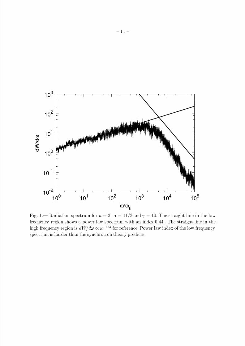
First, we show the radiation spectrum for a = 3 in Figure 1. The frequency is normalized

by the fundamental frequency ωg = eσ/(γmc), and the magnitude is arbitrarily scaled. The

jagged line is the calculated spectrum, while the straight line drawn in the low frequency

region is a line fitted to a power law spectrum. The fitting is made in the range of 1− 350ωg

and the spectral index turns out to be 0.44. The straight line drawn in the high frequency

region shows a spectrum of ∝ ω−5/3 expected for diffusive synchrotron radiation for reference

(Toptygin & Fleishman 1987). The spectrum is well described by a broken power law, and

the spectral index of the low energy side is harder than synchrotron theory predicts. The

peak frequency of this spectrum is located at around 103ωg. This frequency corresponds to

approximately the typical frequency of synchrotron radiation ωsyn = 3γ 2eσ/2mc ∼ 103ωg,

for γ = 10.

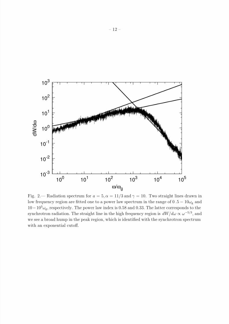
Figure 2 shows the spectrum for a = 5. The spectral shape changes from that of a = 3

in both sides of the peak. The spectrum of the low frequency side becomes a broken power

law with a break around 10ωg, above which the spectrum is fitted by a power law with an

index of 0.33, as expected for synchrotron radiation, while below the break the index is 0 .58.

8/6/2019 To Read 1106


8/6/2019 To Read 1106


– 7 –

for a < 1, if we consider that the middle frequency region is not conspicuous. Although

our spectral index 0.44 slightly differs from 0.5 for DSR, this index is still harder than the

synchrotron theory. The situation a ∼ 1 can be achieved at the internal shock region of GRB, so that this may be responsible for harder spectral index than synchrotron observed

for some GRBs.

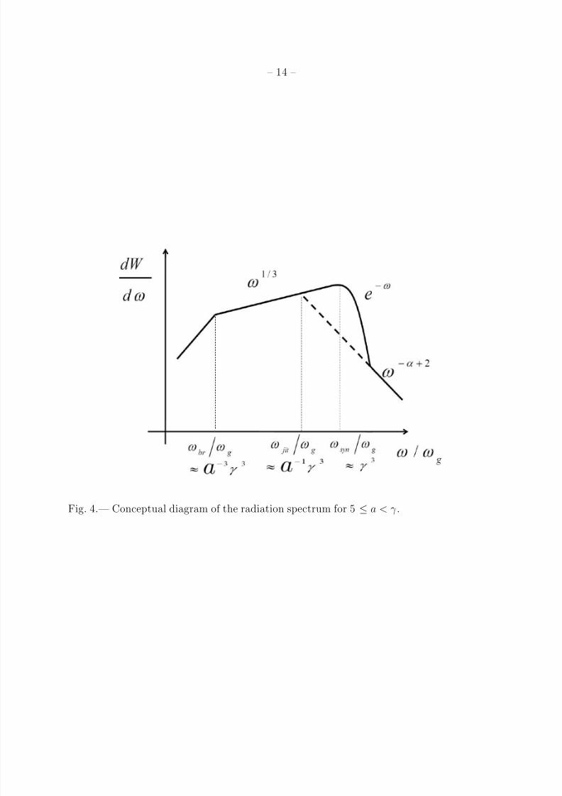
Next we interpret the spectral features for a = 5 and 7. The conceptual diagram of

these spectra for 5 ≤ a < γ is depicted in Figure 4, and a schematic picture of an electron

trajectory is depicted in Figure 5. We explain the appearance of another break in the low

frequency range seen at around 10ωg in Figure 2. On the scale smaller than λB, the electron

motion may be approximated by a helical orbit, while it is regarded as a randomly fluctuating

trajectory when seen on scales larger than λB. Therefore, for the former scale, we can apply

the synchrotron approximation to the emitted radiation. The beaming cone corresponding

to the frequency ω is given by

θcone =1

γ (

3ωsyn

ω)1/3 (13)

(Jackson 1999). The deflection angle θ0 of the electron orbit during a time λB/c is estimated

to be θ0 = a/γ from the conditionγλB

aθ0 = λB (14)

as seen in Figure 5. Thus, the synchrotron theory is applicable only for θcone < θ0, so that

the break frequency is determined by θ0 = θcone, and we obtain

ωbr ∼ a−3ωsyn. (15)

This break frequency is the same as obtained by Medvedev (Medvedev 2010). We understand

that as a is larger, break frequency becomes lower, and when a is comparable to γ , ωbr

coincides with the fundamental frequency eσ/γmc.

Next, we discuss on the high frequency radiation, which results from the electron tra-

jectory on scales smaller than λB. The synchrotron theory applies between λB/a = rg/γ

and λB. However, we should notice that electron motion suffers from acceleration by mag-

netic turbulence on scales smaller than λB/a. The trajectory down to the smallest scale of

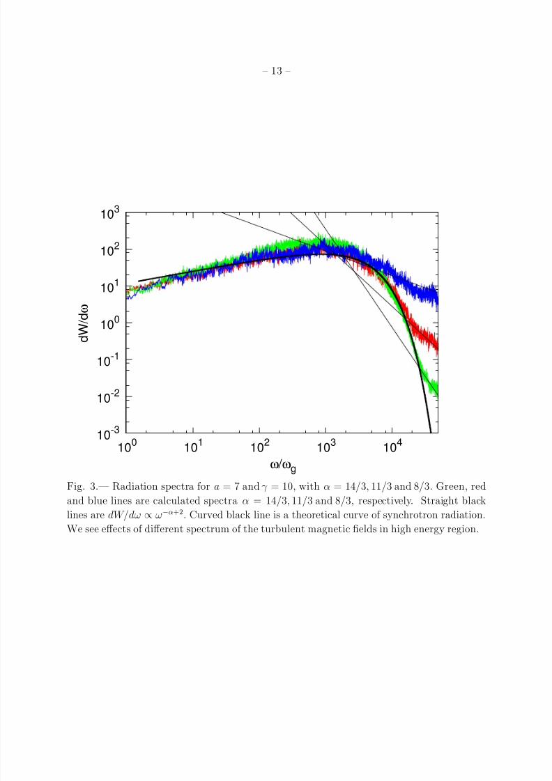
2π/kmax is jittering, which is attributed to higher wavenumber modes as seen in the zoom upof Figure 5. If the field in this regime is relatively weak, i.e., α is relatively large (Figure 3,

green line: α = 14/3), the trajectory on the scale smaller than λB/a does not much deviate

from a helical orbit. In this case, radiation spectrum reveals an exponential cutoff, and a

power law component appears only in the highest frequency region. On the contrary, if the

smaller scale field is relatively strong, as in the case of α = 8/3 depicted in the blue line

in Figure 3, the power law component becomes predominant in the high frequency region,

8/6/2019 To Read 1106


– 8 –

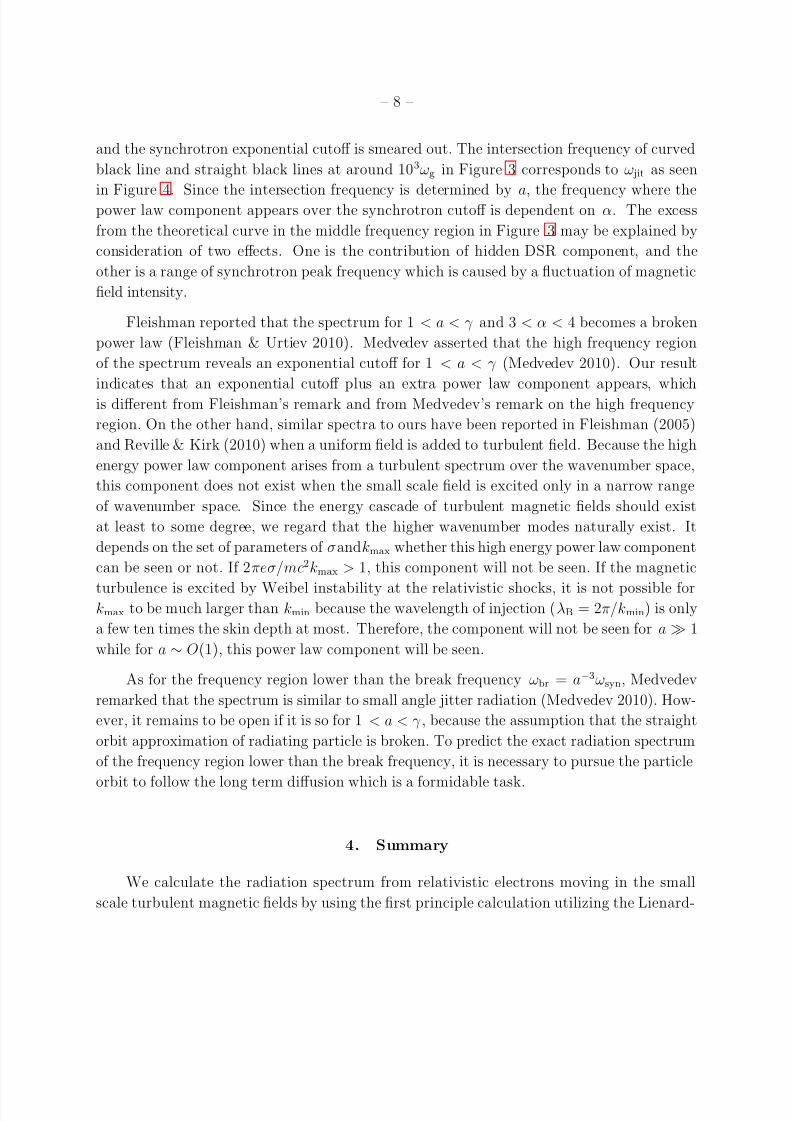
and the synchrotron exponential cutoff is smeared out. The intersection frequency of curved

black line and straight black lines at around 103ωg in Figure 3 corresponds to ω jit as seen

in Figure 4. Since the intersection frequency is determined by a, the frequency where thepower law component appears over the synchrotron cutoff is dependent on α. The excess

from the theoretical curve in the middle frequency region in Figure 3 may be explained by

consideration of two effects. One is the contribution of hidden DSR component, and the

other is a range of synchrotron peak frequency which is caused by a fluctuation of magnetic

field intensity.

Fleishman reported that the spectrum for 1 < a < γ and 3 < α < 4 becomes a broken

power law (Fleishman & Urtiev 2010). Medvedev asserted that the high frequency region

of the spectrum reveals an exponential cutoff for 1 < a < γ (Medvedev 2010). Our result

indicates that an exponential cutoff plus an extra power law component appears, which

is different from Fleishman’s remark and from Medvedev’s remark on the high frequency

region. On the other hand, similar spectra to ours have been reported in Fleishman (2005)

and Reville & Kirk (2010) when a uniform field is added to turbulent field. Because the high

energy power law component arises from a turbulent spectrum over the wavenumber space,

this component does not exist when the small scale field is excited only in a narrow range

of wavenumber space. Since the energy cascade of turbulent magnetic fields should exist

at least to some degree, we regard that the higher wavenumber modes naturally exist. It

depends on the set of parameters of σandkmax whether this high energy power law component

can be seen or not. If 2πeσ/mc2kmax > 1, this component will not be seen. If the magnetic

turbulence is excited by Weibel instability at the relativistic shocks, it is not possible forkmax to be much larger than kmin because the wavelength of injection (λB = 2π/kmin) is only

a few ten times the skin depth at most. Therefore, the component will not be seen for a ≫ 1

while for a ∼ O(1), this power law component will be seen.

As for the frequency region lower than the break frequency ωbr = a−3ωsyn, Medvedev

remarked that the spectrum is similar to small angle jitter radiation (Medvedev 2010). How-

ever, it remains to be open if it is so for 1 < a < γ , because the assumption that the straight

orbit approximation of radiating particle is broken. To predict the exact radiation spectrum

of the frequency region lower than the break frequency, it is necessary to pursue the particle

orbit to follow the long term diffusion which is a formidable task.

4. Summary

We calculate the radiation spectrum from relativistic electrons moving in the small

scale turbulent magnetic fields by using the first principle calculation utilizing the Lienard-

8/6/2019 To Read 1106


– 9 –

Wiechert potential. We concentrate our calculation on a range of the strength parameter of

1 < a < γ . We confirm that the spectrum for a ∼ 3 is a broken power law with an index

of low energy side ∼ 0.5, and that some GRBs with low energy spectral index harder thansynchrotron theory predicts may be explained. Furthermore, we find that the spectrum for

a ∼ 7 takes a novel shape described by a superposition of a broken power law spectrum and a

synchrotron one. Especially, an extra power law component appears beyond the synchrotron

cutoff in the high frequency region reflecting magnetic field fluctuation spectrum. This is

in contrast with previous works (Fleishman & Urtiev 2010, Medvedev 2010). Our spectra

for a = 5 and a = 7 are different from both of them. We have given a physical reason

for this spectral feature. This novel spectral shape may be seen in various other scenes in

astrophysics. For example, the spectrum of 3C273 jet at the knot region may be due to this

feature (Uchiyama et al. 2006).

We thank the referee for helpful comments. We are grateful to T. Okada, S. Tanaka, M.

Yamaguchi for discussion and suggestions. This work is partially supported by KAKENHI

20540231 (F.T.).

REFERENCES

Chang, P., Spitkovsky, A., & Arons, J. 2008, ApJ, 530, 292

Fleishman, G. D. 2005, arXiv:astro-ph/0510317v1

Fleishman, G. D. 2006, ApJ, 638, 348

Fleishman, G. D., & Urtiev, F. A. 2010, MNRAS, 406, 644

Fredediksen, J. T., Hededal, C.B., Haugbolle, T., & Nordlund, A. 2004, ApJ, 608, L13

Frederiksen, J.T., Haugbolle, T., Medvedev, M.V., & Nordlund, A. 2010, ApJ, 722, L114

Giacalone, J., & Jokipii, J. R. 1999 ApJ, 520, 204

Haugbolle, T. 2010, arXiv:astro-ph/1007.5082v1

Hededal, C. 2005, PhD thesis, Nils Bohr Institute, arXiv:astro-ph/0506559

Jackson, J. D. 1999, Classical Electrodynamics (3rd ed.;New York:Wieley)

Kato, T. N. 2005, Physics of Plasmas 12, 080705

Medvedev, M. V., & Loeb, A. 1999, ApJ, 526, 697

http://fr.arxiv.org/abs/astro-ph/0510317




8/6/2019 To Read 1106


– 10 –

Medvedev, M. V. 2000, ApJ, 540, 704

Medvedev, M. V. 2006, ApJ, 637, 869

Medvedev, M. V., Pothapragada, S. S., & Reynolds, S. J. 2009, ApJ, 702, L91

Medvedev, M. V. 2010, arXiv: astro-ph/1003.0063v2

Nishikawa, K. -I. et al 2011, Adv. Space Res. 47, 1134

Reville, B., & Kirk, J. G. 2010 ApJ, 724, 1283R

Rybicki, R. D., & Lightman, A. D. 1979, Radiative Processes in Astrophysics (New York:

Willey)

Sironi, L., & Spitkovsky, A. 2009, ApJ, 707, L92

Toptygin, I. N., & Fleishman, G. D. 1987, Ap&SS. 133,213T

Uchiyama, Y. et al. 2006, ApJ, 648, 910

This preprint was prepared with the AAS LATEX macros v5.2.

8/6/2019 To Read 1106


– 11 –

10-2

10-1

100

101

102

103

100

101

102

103

104

105

d W / d ω

ω / ωg

Fig. 1.— Radiation spectrum for a = 3, α = 11/3 and γ = 10. The straight line in the low

frequency region shows a power law spectrum with an index 0.44. The straight line in the

high frequency region is dW/dω ∝ ω−5/3 for reference. Power law index of the low frequency

spectrum is harder than the synchrotron theory predicts.

8/6/2019 To Read 1106


– 12 –

10-3

10-2

10-1

100

101

102

103

100

101

102

103

104

105

d W / d ω

ω / ωg

Fig. 2.— Radiation spectrum for a = 5, α = 11/3 and γ = 10. Two straight lines drawn in

low frequency region are fitted one to a power law spectrum in the range of 0 .5− 10ωg and

10−103ωg, respectively. The power law index is 0.58 and 0.33. The latter corresponds to the

synchrotron radiation. The straight line in the high frequency region is dW/dω ∝ ω−5/3, and

we see a broad hump in the peak region, which is identified with the synchrotron spectrum

with an exponential cutoff.

8/6/2019 To Read 1106


– 13 –

10-3

10-2

10-1

100

101

102

103

100

101

102

103

104

d W / d ω

ω / ωg

Fig. 3.— Radiation spectra for a = 7 and γ = 10, with α = 14/3, 11/3 and 8/3. Green, red

and blue lines are calculated spectra α = 14/3, 11/3 and 8/3, respectively. Straight black

lines are dW/dω ∝ ω−α+2. Curved black line is a theoretical curve of synchrotron radiation.

We see effects of different spectrum of the turbulent magnetic fields in high energy region.

8/6/2019 To Read 1106


– 14 –

Fig. 4.— Conceptual diagram of the radiation spectrum for 5 ≤ a < γ .

8/6/2019 To Read 1106


– 15 –

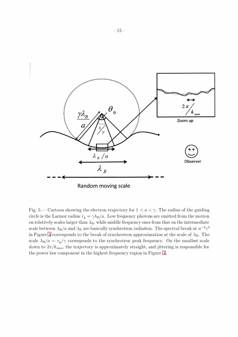
Fig. 5.— Cartoon showing the electron trajectory for 1 < a < γ . The radius of the guiding

circle is the Larmor radius rg = γλB/a. Low frequency photons are emitted from the motion

on relatively scales larger than λB, while middle frequency ones from that on the intermediate

scale between λB/a and λB are basically synchrotron radiation. The spectral break at a−3γ 3

in Figure 4 corresponds to the break of synchrotron approximation at the scale of λB. Thescale λB/a = rg/γ corresponds to the synchrotron peak frequency. On the smallest scale

down to 2π/kmax, the trajectory is approximately straight, and jittering is responsible for

the power law component in the highest frequency region in Figure 4.

To Read 1106

Documents

Transcript of To Read 1106