Title DOI Doc URL … PANGKEP Regency, Spermonde Archipelago .....36 Table 2.9 Results of the...
129
Instructions for use Title Assessment of coral reef degradation and the economic loss in the Pangkajene and Kepulauan Regency, Spermonde Archipelago, Indonesia Author(s) Yasir Haya, La Ode Muhammad Issue Date 2017-09-25 DOI 10.14943/doctoral.k12861 Doc URL http://hdl.handle.net/2115/67653 Type theses (doctoral) File Information LaOde_Muhammad.pdf Hokkaido University Collection of Scholarly and Academic Papers : HUSCAP
Transcript of Title DOI Doc URL … PANGKEP Regency, Spermonde Archipelago .....36 Table 2.9 Results of the...

Instructions for use
Title Assessment of coral reef degradation and the economic loss in the Pangkajene and Kepulauan Regency, SpermondeArchipelago, Indonesia
Author(s) Yasir Haya, La Ode Muhammad
Issue Date 2017-09-25
DOI 10.14943/doctoral.k12861
Doc URL http://hdl.handle.net/2115/67653
Type theses (doctoral)
File Information LaOde_Muhammad.pdf
Hokkaido University Collection of Scholarly and Academic Papers : HUSCAP
1
Assessment of coral reef degradation and the economic loss
in the Pangkajene and Kepulauan Regency,
Spermonde Archipelago, Indonesia
(インドネシア・スペルモンデ諸島パンカジェネ・ケプラウワン県における
サンゴ礁の劣化及びその経済損失の評価)
LA ODE MUHAMMAD YASIR HAYA
DOCTORAL DISSERTATION
Division of Environmental Science Development
Graduate School of Environmental Science
Hokkaido University, Japan
2017

2
i
Abstract
Destruction of coral reefs at global scale stays at an alarming rate for decades due to
multiple stressors. There is no exception for coral reefs in the Pangkajene and Kepulauan
(PANGKEP) Regency in the Spermonde Archipelago, Indonesia which is located in the Indo-
Pacific Coral Triangle. They have been under the stresses caused by various harmful impacts.
Since human activities, as well as natural disturbances, posed major threats to the coral reefs,
these livelihoods may also be at risk. Currently, no comprehensive information on the status
and condition of coral reefs in this area is available for this resource management.
This research was conducted to identify the extent of coral damage by using remote
sensing and in-situ measurement data to analyze the changes in coral reefs. This study was
determined the changes in coral habitats over a period of 20 years from 1994 to 2014 using
multi-temporal Land Satellite (Landsat) image data substantiated with in-situ measurement
data collected in 2014. The results show that there has been a decline in live coral cover for 20
years, from 7,716 ha in 1994 to 4,236 ha in 2014, with a destruction rate of 174 ha/yr. The
ratio of the coral cover in the coral reef transects varied from averagely 24% for live corals to
96% for coral rubbles. The decline in live coral habitats is considered to be caused mainly by
destructive fishing practice, followed by excessive total suspended solids in surface waters.
The total economic values of coral reefs in the study area were also estimated by the
sum of the direct use, non-use, and existence values. The total economic value in 2014 was
estimated to be USD 12 billion or 3 million USD/ha, which were related to fisheries, tourism,
recreation, research, coastal protection, existence value and bequest value. While the total
economic value is considered to be still high, this study indicates that the value has been lost
by USD 1 billion or 50 million USD/yr for the 20 years since 1994. The economic loss was
resulting from loss values of coral reefs, including economic losses of fisheries (i.e., coral
fishes, crabs, squids, octopuses and seaweeds), tourism, recreation, and coastal protection. The
economic loss of coral reefs is anticipated to continue in future. Therefore, in order to save
coral reef ecosystems, the local governments of the PANGKEP Regency need to develop and
implement the comprehensive strategic policies, to take protective measures of coral reefs such
as by designing new marine protected areas (MPAs).

ii
List of Contents
Abstract ....................................................................................................................................... i
List of Contents .......................................................................................................................... ii
List of Tables ............................................................................................................................ iv
List of Figures ........................................................................................................................... vi
Chapter I. Introduction .............................................................................................................. 1
1.1 Background: Coral reefs in Indonesia .................................................................................. 1
1.2 Study area............................................................................................................................. 4
1.3 Objectives and Overview of Dissertation ............................................................................ 4
Chapter II. Mapping the change of coral reefs using remote sensing and in situ measurements
in the Pangkajene and Kepulauan Regency, Spermonde Archipelago, Indonesia .................... 7
2.1 Introduction .......................................................................................................................... 7
2.2 Materials and Methods ......................................................................................................... 9
2.2.1 Data sources ................................................................................................................ 9
2.2.2 Image processing ...................................................................................................... 11
2.3 Results ................................................................................................................................ 16
2.3.1 Status of coral reefs .................................................................................................. 16
2.3.2 Image processing ...................................................................................................... 18
2.3.3 TSM detection .......................................................................................................... 18
2.3.4 Water column correction .......................................................................................... 20
2.3.5 Unsupervised classification, reclassification and ground truthing ........................... 20
2.3.6 Accuracy assessment ................................................................................................ 22
2.3.7 Change in coral reef habitat ...................................................................................... 23
2.4 Discussion .......................................................................................................................... 24
2.5 Conclusions ........................................................................................................................ 25
Chapter III. Economic assessment of the benefits and losses of goods and services derived from
coral reefs: a case study in the Pangkajene and Kepulauan Regency, Spermonde Archipelago,
Indonesia .................................................................................................................................. 55
3.1 Introduction ........................................................................................................................ 55
3.2 Materials and Methods ....................................................................................................... 57
3.2.1 Data source and materials ......................................................................................... 57
3.2.2 Framework valuation of the total economic value ................................................... 58
3.2.3 Economic losses of coral reef destruction ................................................................ 62
3.3 Results and Discussion ...................................................................................................... 63
3.3.1 Use values (UVs) of coral reefs ................................................................................ 64
3.3.2 Non-use values (NUVs) of coral reefs ...................................................................... 66

iii
3.3.3 Total economic value (TEV) of coral reefs .............................................................. 67
3.3.4 Total economic loss (TEL) of coral reefs ................................................................. 68
3.4 Conclusion ......................................................................................................................... 69
Chapter IV. General Discussion .............................................................................................. 76
4.1 Threats on coral reefs in the PANGKEP Regency ............................................................ 76
4.2 Value of coral reefs in the PANGKEP Regency ............................................................... 78
4.3 Designing effective marine protected areas (MPAs) ......................................................... 79
4.4 Future perspective of the study .......................................................................................... 80
Chapter V. General Conclusion .............................................................................................. 83
Acknowledgments.................................................................................................................... 85
References ................................................................................................................................ 87
Appendices ............................................................................................................................. 102
Appendix A1. Questionnaire sheet and list interview of the coral reefs in the Pangkajene and
Kepulauan (PANGKEP) Regency, Spermonde Archipelago, Indonesia ............................... 102
Appendix A2. Effect on production (EOP) method ............................................................... 113
Appendix A3. Calculation of direct use values (DUVs) using the effect on production (EOP)
method.................................................................................................................................... 116
Appendix A4. Calculation of existence value of coral reefs using contingency valuation method
(CVM) .................................................................................................................................... 119
iv
List of Tables
Table 2.1 Types and characteristics of Landsat images used in this study. Multi-temporal
Landsat imagery data were obtained from the United States Geological Survey
(2014) ............................................................................................................................27
Table 2. 2 Classification of benthos in the PIT method ...........................................................28
Table 2.3 Coral cover (%) as a guidance of categorization defined by Gomez and Yap (1988)
.......................................................................................................................................29
Table 2.4 Description of classifications. Visually, the coral reef could be sorted into 2
categories (live and dead coral) according to their color. The live coral is generally found
far from land, close to the deep water zone, while dead coral is commonly distributed
close to the shoreline (COREMAP 2001, cited in Suwargana 2014) ...........................30
Table 2.5 Example of the confusion matrix calculation (from Congalton and Green 2008). In
this matrix, Nij is the number of samples classified, where i, j, k and + are the row in the
remotely sensed classification and the column in the reference data set (field data), k is
the next sample number, + is the total of samples in column or row, respectively. In this
case, each column (field data) of the matrix represents the instances in a predicted class
while each row (image classification) represents the instances in an actual class and vice
versa...............................................................................................................................31
Table 2.6 Status of coral reefs in study site based on the result of PIT method at 23 transects in
10 islands .......................................................................................................................32
Table 2.7 Distance of fishing locations from the mainland (before and in 2014) in the study
site. The number in columns of "Before 2014" and "In 2014" were the number of
fisherman who chose favorite locations for fishing in the period of before 2014 and in
2014, respectively ..........................................................................................................34
Table 2.8 The maximum TSM concentration estimated from the multi-temporal Landsat
imagery data in dry (April-Sept.) and rainy (Oct.-March) seasons in the inner zone of
the PANGKEP Regency, Spermonde Archipelago .......................................................36
Table 2.9 Results of the classification of coral reefs and seabed habitats estimated by the multi-
temporal Landsat imagery data in the PANGKEP Regency, Spermonde Archipelago,
Indonesia .......................................................................................................................37
Table 2.10 Confusion matrix value on the classification of four classes of the seabed habitats
in the PANGKEP Regency, Spermonde Archipelago, Indonesia .................................38
Table 2.11 Ratio of producer's accuracy (PA) and the user's accuracy (UA). The calculation
was conducted for four marine habitat classifications in the PANGKEP Regency,
Spermonde Archipelago, Indonesia. Reference data mean the classes which are
classified correctl ...........................................................................................................39

v
Table 2.12 Change in the area of coral reefs from 1994 to 2014 in the PANGKEP Regency,
Spermonde Archipelago, Indonesia. The change of area in each class was established
based on the overlay of coral reef distribution and condition map derived from Landsat
5 TM (1994), Landsat 7 ETM (2002), and Landsat 8 OLI (2014) images ...................40
Table 3.1 Direct use benefits of coral reef-related fisheries calculated using the effect on
production (EOP) method. The calculation is presented in detail in Appendix
A2 ..................................................................................................................................71
Table 3.2 Components of tourist expenditure for visitors to the Kapoposang Marine Park and
Panambungan Island in 2014 ........................................................................................72
Table 3.3 Estimated economic value of coral reefs in the study area based on the categorization
of the economic value of coral reefs in the PANGKEP Regency, Spermonde
Archipelago, Indonesia. The area of coral reefs was fixed to 4,236 ha in 2014
.......................................................................................................................................73
Table 3.4 Estimated current values of economic loss (USD) due to the destruction of coral reefs
from 1994 to 2014 in the PANGKEP Regency, Spermonde Archipelago, Indonesia. The
GDP Implicit Price Deflator (Organization for Economic Co-operation and
Development (OECD), 2016) was used, and a discount rate of 10% was applied for the
estimation. The destruction rate and economic loss of coral reefs was assumed to be 174
ha/yr and 819,500 USD, respectively, during the study period ....................................74
vi
List of Figures
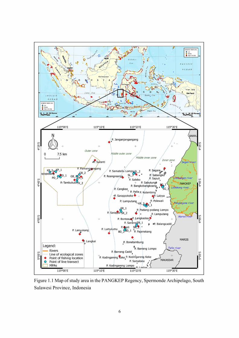
Figure 1.1 Map of study area in the PANGKEP Regency, Spermonde Archipelago, South
Sulawesi Province, Indonesia ........................................................................................6
Figure 2.1 Categories used in PIT method. AC: Acropora; NA: Non-Acropora; SP: Sponge; R:
Rubble; SC: Soft coral; SA: Sand; DCA: Dead coral algae; A: Abiotic. In this case, the
rubble was classified as dead corals .............................................................................41
Figure 2.2 Flowchart research on mapping and analysis of changes in coral reefs .................42
Figure 2.3 Ratio of live corals and dead corals at all sites in the PANGKEP Regency,
Spermonde Archipelago, Indonesia. The graph summarizes the calculation for each
category obtained by PIT method in each village (2-3 observation transects per village)
......................................................................................................................................43
Figure 2.4 Averaged ratio of coral rubbles to total dead corals in the villages in the PANGKEP
Regency, Spermonde Archipelago, Indonesia .............................................................44
Figure 2.5 Ratio of preferred destructive fishing areas (%) obtained by analyzing the results of
questionnaires distributed to 296 respondents, which were strongly linked to the fishing
gears used and target fish species frequently caught ...................................................45
Figure 2.6 Spectral profile of object classes (sand, seagrasses, dead corals, live corals and sea
water) on three series Landsat Imagery data: (a) Landsat TM 1994, (b)
Landsat 7 ETM 2002, and (c) Landsat 8 OLI 2014 .....................................................46
Figure 2.7 Distribution and concentration of total suspended matter (TSM) of the two seasons
in the inner zone: a) dry season in the Landsat 5 TM, 1994; b) dry season in the Landsat
7 ETM, 2002; c) dry season in the Landsat 8 OLI, 2014; d) rainy season in the Landsat
5 TM, 1994; e) rainy season in the Landsat 7 ETM, 2002; f) rainy season in the Landsat
8 OLI, 2014 ..................................................................................................................47
Figure 2.8 Average monthly rainfall in 1994, 2002 and 2014 in the study area (Source: The
modern-era retrospective analysis for research and applications, Version 2; MERRA-
2) ..................................................................................................................................48
Figure 2.9 Plots of spectral values of the coral reef status obtained by three series of multi-
temporal Landsat imagery ((a)-(c) for Landsat 5 TM, 1994; (d)-(f) for Landsat 7 ETM,
2002; (g)-(i) for Landsat 8 OLI, 2014) in the PANGKEP Regency, Spermonde
Archipelago, Indonesia. (a) and (d): Band 2 vs. Band 3; (b) and (e): Band 1 vs. Band 3,
(c), (f) and (g): Band 2 vs. Band 3; (h): Band 2 vs. Band 4; (i) Band 3 vs. Band 4 ....49
Figure 2.10 Depth invariant index derived from three series of multi-temporal Landsat imagery
data ((a)-(c) for Landsat 5 TM, 1994; (d)-(f) for Landsat 7 ETM, 2002; (g)-(i) for
Landsat 8 OLI, 2014) in the PANGKEP Regency, Spermonde Archipelago, Indonesia,
using gradient of the linier line. (a) and (d): Band 2 vs. Band 3; (b) and (e): Band 1 vs.
vii
Band 3, (c), (f) and (g): Band 2 vs. Band 3; (h): Band 2 vs. Band 4; (i) Band 3 vs. Band
4....................................................................................................................................50
Figure 2.11 Distribution and condition of coral reefs in the PANGKEP, Spermonde
Archipelago, Indonesia, obtained from three series multi-temporal Landsat imagery
data. (a) Landsat 5 TM, 1994; (b) Landsat 7 ETM, 2002; (c) Landsat 8 OLI, 2014 ...51
Figure 2.12 Map of change in bottom substrate in the PANGKEP Regency, Spermonde
Archipelago, Indonesia: (a) from 1994 to 2002 and (b) from 2002 to 2014. The
Kapoposang MPAs is located in the outer zone of the PANGKEP islands which also
experienced a drastic decline in coral reef habitats in this period ...............................52
Figure 2.13 Change in composition of coral reefs from 1994 to 2014. During the period, 45.1%
of the coral reef area has been transformed (left pie chart): 91.6% from live to dead
corals, 7.2% from live corals to sand, and 1.2% from dead corals to sand
(right pie chart) ............................................................................................................53
Figure 2.14 Tidal prediction in the PANGKEP Regency, Spermonde Archipelago, Indonesia
with a coordinate point of observation: 1190 15'36 S and 40 48'36 E. The data is
processed by using the prediction model from
http://www.miz.nao.ac.jp/staffs/nao99/index_En.html. Accessed 10 October 2016 ..54
Figure 3.1 Demand function of the coral reef benefits related to the fisheries using the effect
on production (EOP) method for: (a) the coral reef fish catch, (b) the crab catch, (c) the
squids and octopuses catch and (d) seaweed farming ..................................................75
Figure 4.1 Spillover mechanism in the marine protected area (MPAs) (source: Bohnsack
1990)…………………………………………………………………………… ........82

1
Chapter I Introduction
1.1 Background: Coral reefs in Indonesia
Coral reefs are one of the foremost productive ecosystems in the marine
environment and represent high benefit values for human as a source of income, fisheries
resources, construction materials, tourism and recreation and many others for thousands
of years (Hodgson 1999; McManus 1997; Mumby and Steneck 2008). They also play an
important role in preserving the balance of marine resources, and function as the marine
environmental health indicators (Hourigan et al. 1988; Hein et al. 2015). Coral reef
ecosystems are also utilized as valuable resources for supplying goods and services, such
as fisheries, tourism, scientific research, shoreline protection, and so forth (Moberg and
Folke 1999; Souter and Linden 2000; UNEP 2006; Brander et al. 2007; Tseng et al. 2015).
Detrimental effects in changes of coral reefs at global scale have been for last two
decades, mainly in the Carribean and the Western Atlantic region (Aronson and Precht
2001; Gardner et al. 2003), the Great Barrier Reef (De'ath et al. 2012), as well as the Indo-
Pacific (Bruno and Selig 2007). Currently, anthropogenic threats are the main causal
factors of coral reef destruction that exceed natural threats at the global scale. This
inevitable reality is certainly called for serious protection and preservation of coral reef
resources to minimize the main causal factors by formulating and implementing science-
based policy programs (Salvat 1987; Wilkinson 1992; Roberts 1997). There has not been
any significant consensus on how to formulate a holistic approach to protect and preserve
coral reef ecosystems in a more meaningful way.
Indonesia is a tropical country that is located in the center of the Coral Triangle
of the greatest marine biodiversity on earth together with the Philippines, Malaysia,
Timor-Leste, Papua New Guinea and the Solomon Islands. The Coral Triangle region
have the area of approximately 75,000 km2 of coral reefs and contain nearly 600 different
species of reef-building corals alone. More than 120 million people live so dependently
on coral reefs in the region (http://www.worldwildlife.org/publications/stewarding-
biodiversity-and-food-security-in-the-coral-triangle-achievements-challenges-and-
lessons-learned). Indonesia’s coral reefs are approximately 50,875 km2 in the area and
cover 18% of the world’s coral reefs (World Resource Institute (WRI) 2002). In addition,
Indonesia's coral reefs are the most biologically productive in the world, which consists
of an incredibly diverse array of flora and fauna. Today, more than 480 species of hard
corals have been recorded in the eastern Indonesia which accounts for about 60% of the
world's species of hard corals described (Suharsono and Purnomohadi 2010). The highest

2
diversity of coral reef fish is found in Indonesia, with more than 1,650 species in the
eastern Indonesia only. In fact, Indonesia's coral reefs are a supporter of one of the world's
largest marine fisheries, producing 3.6 million tonnes of the total marine fish production
in 1997. Because of many reefs in the eastern Indonesia have yet to be surveyed, so the
actual extent of Indonesia’s biodiversity is still unknown for certain. (Hopley and
Suharsono 2000). However, Indonesia's rich supplies of corals and reef fish are
endangered by unsustainable fishing practices (Radjawali 2012).
Coral reef destruction at global and regional scales as depicted above is
compatible with the local condition in the Pangkajene and Kepulauan (PANGKEP)
Regency, Spermonde Archipelago, as a part of eastern Indonesia’s coral reef zone. Coral
reefs in this archipelago experienced serious threats due to anthropogenic causes as shown
in both direct and indirect activities of the local communities (DFW-Indonesia 2003; Pet-
Soede 2000) and natural causes that include the impact of climate changes (Yusuf and
Jompa 2012). The main causal factors of coral reef destruction in this archipelago are
unsustainable fishing activities such as the use of bombs and cyanide. These devices have
causes a double impact, not only the damage to coral reefs but also the death of marine
species that rely on the coral reefs (Pet-Soede 2000; DFW-Indonesia 2003).
Human activities, including agricultural and pond farming activities, produce
pollutant, such as sewage, pesticides, and organic and anorganic fertilizers. These
pollutants are usually discharged into the sea waters that lead to harmful impacts on coral
reef ecosystems and other living organisms (Fabricius 2005; D’Angelo and Wiedenmann
2014). Several activities carried out by the local communities in the PANGKEP and
Maros Regencies such as uncontrolled deforestation and lime mining are considered to
contribute to the erosion of soil surface layers and occurrence of harmful materials at a
high rate through sedimentation that runs into the sea waters and local estuaries
(Augustinus 2001). Total suspended matters (TSM) in the sedimentation that cover
polyps of coral reefs trigger stresses to coral reefs which leads to death of corals (Davies-
Colley and Smith 2000; Jones et al. 2015).
On the other hand, global increase of seawater temperature threatens coral reefs
through bleaching process. In the mid-February to March 2016, this phenomenon was
identified in several observation sites in Badi, Bontosua and Sanane Islands. The water
temperature was 3oC higher than the climatology of 29oC (Syafyuddin Yusuf of
Hasanuddin University, per. comm.). In this case, bleaching rapidly proceeded in most of
the coral reefs in 7 through 15 m depth, while the bleaching was not detected in coral
reefs in shallow water of 1-5 m depth. This is probably caused by higher ability of shallow
coral reefs to adapt to the higher temperature condition. In general, it is estimated that
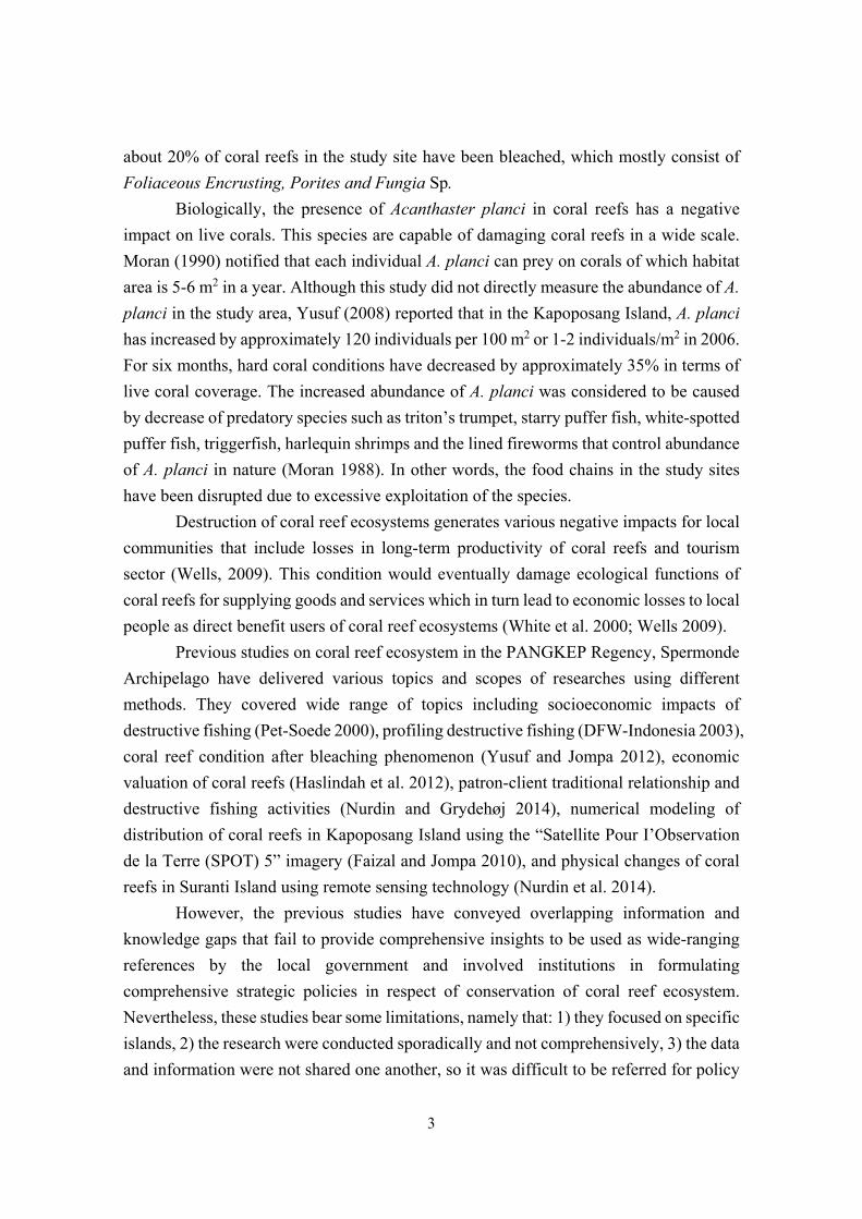
3
about 20% of coral reefs in the study site have been bleached, which mostly consist of
Foliaceous Encrusting, Porites and Fungia Sp.
Biologically, the presence of Acanthaster planci in coral reefs has a negative
impact on live corals. This species are capable of damaging coral reefs in a wide scale.
Moran (1990) notified that each individual A. planci can prey on corals of which habitat
area is 5-6 m2 in a year. Although this study did not directly measure the abundance of A.
planci in the study area, Yusuf (2008) reported that in the Kapoposang Island, A. planci
has increased by approximately 120 individuals per 100 m2 or 1-2 individuals/m2 in 2006.
For six months, hard coral conditions have decreased by approximately 35% in terms of
live coral coverage. The increased abundance of A. planci was considered to be caused
by decrease of predatory species such as triton’s trumpet, starry puffer fish, white-spotted
puffer fish, triggerfish, harlequin shrimps and the lined fireworms that control abundance
of A. planci in nature (Moran 1988). In other words, the food chains in the study sites
have been disrupted due to excessive exploitation of the species.
Destruction of coral reef ecosystems generates various negative impacts for local
communities that include losses in long-term productivity of coral reefs and tourism
sector (Wells, 2009). This condition would eventually damage ecological functions of
coral reefs for supplying goods and services which in turn lead to economic losses to local
people as direct benefit users of coral reef ecosystems (White et al. 2000; Wells 2009).
Previous studies on coral reef ecosystem in the PANGKEP Regency, Spermonde
Archipelago have delivered various topics and scopes of researches using different
methods. They covered wide range of topics including socioeconomic impacts of
destructive fishing (Pet-Soede 2000), profiling destructive fishing (DFW-Indonesia 2003),
coral reef condition after bleaching phenomenon (Yusuf and Jompa 2012), economic
valuation of coral reefs (Haslindah et al. 2012), patron-client traditional relationship and
destructive fishing activities (Nurdin and Grydehøj 2014), numerical modeling of
distribution of coral reefs in Kapoposang Island using the “Satellite Pour I’Observation
de la Terre (SPOT) 5” imagery (Faizal and Jompa 2010), and physical changes of coral
reefs in Suranti Island using remote sensing technology (Nurdin et al. 2014).
However, the previous studies have conveyed overlapping information and
knowledge gaps that fail to provide comprehensive insights to be used as wide-ranging
references by the local government and involved institutions in formulating
comprehensive strategic policies in respect of conservation of coral reef ecosystem.
Nevertheless, these studies bear some limitations, namely that: 1) they focused on specific
islands, 2) the research were conducted sporadically and not comprehensively, 3) the data
and information were not shared one another, so it was difficult to be referred for policy

4
planning, 4) the information related to multidimensional threats to the coral reefs were
limited.
Considering the problems as stated above, this study aims to analyze three
essential aspects related to direct roles of coral reefs and their environment that includes
physical changes of coral reef habitats, socioeconomic aspects of coral reefs in the local
community, and formulation of alternative strategic policies in managing coral reefs to
look for more significant efforts in improving the status of coral reefs in the study area.
1.2 Study area The study was carried out in the PANGKEP Islands, Spermonde Archipelago,
South Sulawesi Province, Indonesia (Figure 1.1). Geographically, the sites were situated
within 118o54’36”E - 119o35’24”E and 4o30’36”S - 5o03’48”S. Administratively, there
are 41 islands (including 31 islands inhabited) that consist of two districts of Liukang
Tuppabiring and Tuppabiring Utara (Statistics Indonesia of Pangkajene and Kepulauan
Regency 2014). Along the coastal area from Makassar City to the PANGKEP Regency,
there are six rivers and five of them are active rivers all the year around. Ecologically,
corals in the Spermonde Archipelago including those in the PANGKEP Regency are
classified into four ecological zones (Hoeksema 2012), namely inner zone that contains
muddy sand as a bottom substrate, followed by middle inner zone which contains many
coral islands, middle outer zone of which coral reef areas are still submerged, and outer
zone as a barrier reef zone which contains coral islands (Figure 1.1).
Since 1994, 50,000 ha of the outer islands in the PANGKEP Regency have been
designated as marine protected areas (MPAs) by the decrees of the Minister of Forestry
No. 588/Kpts-VI/1996 and the Minister of Marine and Fisheries No. 66/MEN/2009
(Figure 1.1). In addition, this site is within the coral reef rehabilitation and management
program (COREMAP) location which was implemented from 2004 to 2010. Since then,
the exploitation and use of coral reefs have been restricted to ensure the sustainable
management.
1.3 Objectives and Overview of Dissertation Considering the problems mentioned above, this study aims to cover several
issues: 1) assessing coral degradation by using in-situ and satellite data, 2) elucidating
causes of the coral degradation by social survey to local stakeholders, 3) estimating values
and losses of the coral reefs by economic evaluation methods, and 4) providing
suggestions and recommendations for saving the coral reefs scientifically based on the
results obtained by this study. Therefore, the general objective of this study is to assess
5
the changes in coral cover for 20 years from 1994 to 2014 and the socioeconomic value
of coral reefs (i.e., economic benefits and economic loss) in the PANGKEP Regency,
Spermonde Archipelago, Indonesia.
This dissertation consists of five chapters. The following chapter illustrates the
analysis of coral cover changes in the last 20 years from 1994 to 2014 in the PANGKEP
Regency, Spermonde Archipelago, using several sets of data that consist of data of multi-
temporal Land Satellite (LANDSAT) imagery, ground truth, coral reef transect and social
survey. Based on the results obtained in Chapter II, economic benefit values and
economic loss values of the coral reefs in the study site were estimated, as described in
Chapter III. Chapter IV contains a general discussion to bridge the results of this study
and recommendations for future policy making. The last chapter sets forth summary and
conclusion of the overall results of Chapters I through IV.
6
Figure 1.1 Map of study area in the PANGKEP Regency, Spermonde Archipelago, South
Sulawesi Province, Indonesia

7
Chapter II Mapping the change of coral reefs using remote sensing and in situ
measurements in the Pangkajene and Kepulauan Regency, Spermonde Archipelago, Indonesia
2.1 Introduction Coral reefs have been exploited as resources for income, fisheries, construction
materials, tourism and recreational and other purposes for thousands of years (Hodgson
1999; McManus 1997; Mumby and Steneck 2008). Ecologically, coral reefs fulfill an
important role in maintaining the balance of marine resource productivity and serve as
indicators of the health of the marine environment (Hourigan et al. 1988; Hein et al. 2015).
In recent decades, changes in coral reef ecosystems have occurred on both
regional and global scales due to natural effects and anthropogenic factors (Burke et al.
2011; Wilkinson 2008). Burke et al. (2011) reported that more than 60% of the world’s
coral reefs were threatened directly by one or multiple factors, including overfishing,
destructive fishing, coastal development, and environmental pollution. Among these,
overfishing and destructive fishing were the most widely practiced, affecting more than
55% of the world’s coral reefs (Bruno and Selig 2007; Burke et al. 2011). Furthermore,
on a regional scale, the threat of coral reefs occur in the Coral Triangles. Coral Triangles,
lying in Indonesia, the Philippines, Malaysia, Timor-Leste, Papua New Guinea and the
Solomon Islands, are the world's center of marine biodiversity, particularly coral reefs
(World Wild Fund (WWF) 2016).
Since 1998, the Indonesian Government has paid significant attention to manage
coral reef ecosystem through the Coral Reef Rehabilitation and Management Program
(COREMAP). The purpose of this program is protection, rehabilitation and management
focused on the sustainable use of coral reefs and related marine ecosystems in Indonesia,
which in turn will support the welfare of coastal communities (World Bank 2015).
Unfortunately, in some locations, COREMAP has been insignificantly reducing coral reef
exploitation activities, especially in areas outside COREMAP sites. Fishing activities that
threaten coral reef ecosystems continued to be practiced inside some COREMAP
locations, such as Pangkajene and Kepulauan (PANGKEP) Regency in Spermonde
Archipelago, South Sulawesi. The large size of the area and limited resources (equipment
and coral reef data) were considered as major obstacles in monitoring and protecting the
coral reefs. Up-to-date information is essential for designing an effective policy and
management systems to protect coral reefs. One of the methods that could be used to fill
this gap is the use of remote sensing technology.

8
Remote sensing technology has several advantages over other technologies in
terms of providing multi-year databases so that only periodic coral reef field monitoring
is necessary (Goodman et al. 2013; Mumby and Harborne 1999). Remote sensing can be
effectively used to determine the status of coral reefs and has been used by researchers
for scientific investigation, management, and mapping. Roelfsema et al. (2002) used
Landsat Thematic Mapper (TM) imagery to study the spatial distribution of microalgae
in coral reefs. Lubin et al. (2001) measured coral reef and non-coral reef reflectance using
a coupled ocean–atmosphere radiative transfer model and showed that various spectral
features could be used to distinguish coral reefs from the surroundings. The data used as
input are generally obtained from surface or aircraft data, although aircraft data are
generally obscured in terms of spectral measurements. Lubin et al. (2001) support the
conclusion of recent research that the use of satellite remote sensing is effective for coral
reef mapping. Although detailed reef mapping (e.g., species identification) is difficult,
Mumby (2001) developed an explicit method to chart coral species distribution.
The combination of remote sensing and in situ data can be used to verify the
evolution of coral reef degradation, including its recovery over timescales of years to
decades. Scopélitis et al. (2009) identified the typology of coral reef communities using
remote sensing data combined with integrated in situ data between 1973 and 2003 in
Saint-Leu Reef in the Indian Ocean. Five aerial photographs and two QuickBird images
combined with field observations were used to detect the changes in coral reefs during
three impact periods, two caused by storms in 1989 and 2002, and one by coral reef
bleaching in 2002. Scopélitis et al. (2009) concluded that there was no significant change
in the patchy reefs between 1973 and 2006 due to the rapid recovery rate of corals
(Acropora Sp.) from bleaching. Palandro et al. (2008) quantified coral reef degradation
in Florida Keys Natural Marine Sanctuary, USA, from 1984 to 2002, using Landsat
imagery and determined the coral reef destruction to be 61%, or 3.4% /yr. Using different
generations of Landsat imagery, i.e. Landsat 5 TM (1987), Landsat 7 ETM (2000), and
Landsat 8 OLI (2013), with field observation data from 2004, El-Askary et al. (2014)
detected changes in coral reefs in Hurgadha, Egypt. Using supervised classification,
changes in coral reef habitats can be identified qualitatively and quantitatively for specific
periods.
Similar studies have been conducted in Indonesia. Nurdin et al. (2015) have
studied changes in the coral reefs of the coastal area of a small island (Suranti Island) in
the PANGKEP Regency by using multi-temporal Landsat imagery as their primary data
source. However, there are no previous studies that have focused on changes in the coral
reefs of all the islands over the PANGKEP Regency.

9
Additionally, this study was not only used the data from the multi-temporal
Landsat imagery (from the year of 1994 to 2014), but also the in-situ data of the coral reef
habitats monitoring. Purkis and Pasterkamp (2004) reported that the integration of these
data will provide advantages in terms of accuracy, time, cost-effectiveness and coverage
area (Jupiter et al. 2013; Hedley et al. 2016; Mumby et al. 1999; Mumby et al. 2004).
Considering these conditions, to elucidate changes in coral conditions and the
causes in the PANGKEP Regency, it is considered important to analyze large-scale data
as well as limitation of data availability in this area. Therefore, this study aimed to provide
a map of the coral reefs distribution around the area, identify and calculate the changes in
the ratio of coral cover in two decades from 1994 to 2014.
2.2 Materials and Methods 2.2.1 Data sources
2.2.2.1 Satellite Landsat imagery data
This study used Landsat 5 Thematic Mapper (TM), Landsat 7 Enhanced Thematic
Mapper (ETM), and Landsat 8 Operational Land Imager (OLI) multi-temporal imagery,
acquired in 1994, 2002, and 2014, respectively. The analysis of changes in the coral reefs
was performed for a 20-year period, considering the ability of coral reefs to recover from
stress conditions occurring within this period (Wilkinson 2008).
As well as coral cover analysis, this study detected changes in the total suspended
matter (TSM) concentrations in the sea waters using multi-temporal Landsat imagery data
in the same period. The Landsat imagery data used were the Landsat multi-temporal
images that were recorded in different seasons (rainy and dry seasons). The types and
characteristics of the Landsat image are summarized in Table 2.1.
The study area was covered in the same scene in Landsat 5 TM and 7 ETM
(path/row: 114/63), whereas Landsat 8 OLI covered the area in two scenes (path/row:
114/63 and 115/63). The Landsat data had a spatial resolution of 30 m. The Landsat image
acquired in 2002 was chosen to minimize the loss of information due to incomplete data
caused by technical problems during data acquisition. Moreover, the data obtained before
Scan Line Corrector (SLC) turned-off selection were recommended by NASA’s
Millennium Coral Reef Mapping Project (NASA 2009).
2.2.2.2 Data of rainfall
The rainfall data (mm / day) were used to determine the effect of rainfall on the
dynamics of the maximum change of TSM concentration in the waters at two different
seasons (dry and rain) in 1994, 2002, and 2014. In this study, the rainfall data for the 20
10
years from 1994 to 2014 were obtained from the satellite (the Modern-Era Retrospective
analysis for Research and Applications, Version 2; MERRA-2) (https://cds-
cv.nccs.nasa.gov/CREATE-V/). Furthermore, the daily rainfall data were averaged and
compiled as monthly rainfall data.
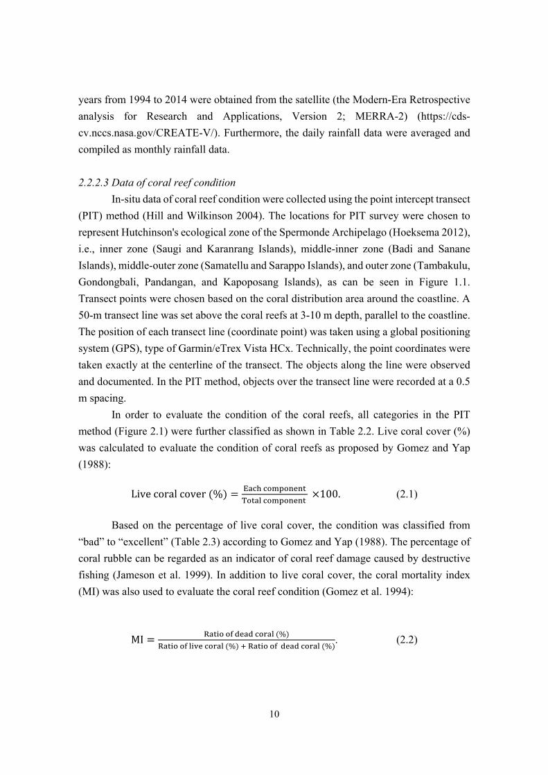
2.2.2.3 Data of coral reef condition
In-situ data of coral reef condition were collected using the point intercept transect
(PIT) method (Hill and Wilkinson 2004). The locations for PIT survey were chosen to
represent Hutchinson's ecological zone of the Spermonde Archipelago (Hoeksema 2012),
i.e., inner zone (Saugi and Karanrang Islands), middle-inner zone (Badi and Sanane
Islands), middle-outer zone (Samatellu and Sarappo Islands), and outer zone (Tambakulu,
Gondongbali, Pandangan, and Kapoposang Islands), as can be seen in Figure 1.1.
Transect points were chosen based on the coral distribution area around the coastline. A
50-m transect line was set above the coral reefs at 3-10 m depth, parallel to the coastline.
The position of each transect line (coordinate point) was taken using a global positioning
system (GPS), type of Garmin/eTrex Vista HCx. Technically, the point coordinates were
taken exactly at the centerline of the transect. The objects along the line were observed
and documented. In the PIT method, objects over the transect line were recorded at a 0.5
m spacing.
In order to evaluate the condition of the coral reefs, all categories in the PIT
method (Figure 2.1) were further classified as shown in Table 2.2. Live coral cover (%)
was calculated to evaluate the condition of coral reefs as proposed by Gomez and Yap
(1988):
Livecoralcover %
100. (2.1)
Based on the percentage of live coral cover, the condition was classified from
“bad” to “excellent” (Table 2.3) according to Gomez and Yap (1988). The percentage of
coral rubble can be regarded as an indicator of coral reef damage caused by destructive
fishing (Jameson et al. 1999). In addition to live coral cover, the coral mortality index
(MI) was also used to evaluate the coral reef condition (Gomez et al. 1994):
MI %
% %. (2.2)

11
2.2.2.4 In-situ ground control point and ground truth data
In addition to the in-situ data obtained by the PIT method, the ground control point
(GCP) and ground truth (GT) coordinate points were determined using a global
positioning system (GPS), type of Garmin/eTrex Vista HCx. Generally, the GCP points
were road intersections, docks, or other landmarks identifiable in the satellite images.
Ground truth data were obtained using GPS for each type of seabed cover, including live
corals, dead corals, seagrasses, and sand. In addition, the GT data were applied to check
the accuracy of the image classification results.
2.2.2.5 Social survey data
In order to ensure the results of primary data analysis, social survey was conducted
to obtain complemental information about fishing activities in the coral reef area, i.e.
fishing location, fishing gear used, destructive fishing activities and so on. In the case of
social survey, questionnaires were distributed to the fishermen and their households
following Krejcie and Morgan (1970)’s method. Based on the population size on ten
inhabited islands, 296 fishermen were chosen as respondents through purposive random
sampling.
2.2.2.6 Secondary data
This study was used a PANGKEP regional administration map (1:250,000) and
Indonesia coastal environmental map (1:250,000) obtained from the Government of
PANGKEP Regency to identify the islands and bathymetry in the study area.
2.2.2 Image processing
In this study, the image processing was carried out in the areas not affected by
turbidity and sedimentation because the sensor is only able to penetrate the turbidity of
the water at a depth of less than 1 m. Based on Hutchinson's ecological zone, reef areas
analyzed include middle inner zone, outer middle zone, and the outer zone (Hoeksema
2012). Image processing consisted of several phases as described the following
subsections.
2.2.2.1 Atmospheric correction
Scattering and absorption of molecules by the atmosphere decreases the quality
of information in the satellite image by up to 10%, depending on the spectral channel
(Che and Price 1992; Ishizaka et al. 1992). Therefore, an atmospheric correction is
12
essential in order to minimize the effect of the atmosphere in multi-temporal images
before comparing and analyzing the data (Hadjimitsis et al. 2010). In this study, an
atmospheric correction was applied to the three series of Landsat imagery data using Dark
Object Subtraction 1 (DOS1) Method (Chavez 1996). For easier atmospheric correction,
this study was applied semi-automatic classification plugin (SCP) in QGIS version 2.10
(Congedo and Macchi 2013).
2.2.2.2 Geometric correction
Geometric correction for Landsat 5 TM and Landsat 7 ETM imagery data was
conducted using the same GCPs on Landsat 8 OLI corrected as a reference. This aims to
improve the accuracy and minimize the geometric error in Landsat imagery data. Eight
GCPs were chosen for the geometric correction using order polynomial transformation
and the nearest neighbor interpolation algorithm (Baboo and Devi 2011). The corrected
image is acceptable if the root mean square error (RMSE) is a one-half pixel wide (RMSE
= 0.5). Overall, the RMSE less than 0.5 pixel were achieved for each transformation.
2.2.2.3 Mosaic image
Mosaicking is a process to merge two or more scenes into a single scene or image.
The process was applied to Landsat 8 OLI imagery data since in this Landsat image, the
study area (PANGKEP in the Spermonde Archipelago) was captured in two scenes
(path/row: 114/63 and 115/63). This is in contrast to previous Landsat imagery data that
require only one scene (path/row: 114/63). Since 2010, Landsat 8 OLI has replaced
previous Landsat versions such as Landsat 7 ETM and Landsat 5 TM. In the mosaicking
process, the digital value of both images needs to be balanced and normalized by using
smooth intensity filter modulation (SFIM) pan sharpen wizard of ER Mapper in order to
increase the spectral qualities of merged images (ERDAS 2008).
2.2.2.4 Subset image (cropping)
Creating a subset image, or “cropping,” aims to delimit the area of interest,
reinforce geospatial phenomenon, and focus on the study area. In addition, the subset
image produces objects that are larger in size, allowing existing information such as color
to be seen more clearly.
2.2.2.5 Image composite (true color)
True color on Landsat 5 TM and Landsat 7 ETM was displayed by using
combination bands of Red: Green: Blue (R: G: B) 3: 2: 1, whereas the color was displayed
13
as R: G: B = 4: 3: 2 on the Landsat 8 Operational Land Imager (OLI). This band
combination is often used to detect feature types covering shallow bottom waters in the
preliminary stage. Chlorophyll in vegetation were detected using green canal (band 2 in
Landsat 5 TM and Landsat 7 ETM, and band 3 in Landsat 8 OLI).
High chlorophyll concentration on the mainland provided a high digital reflection
value and was shown as dark green. Water bodies were detected using band 1 (Landsat 5
TM and 7 ETM) and band 2 (Landsat 8 OLI) in the blue composite so that water bodies
could be depicted in blue.
2.2.2.6 Total Suspended Matter (TSM)
One of the controlling factors for the growth of coral reefs is the total suspended
matter (TSM) concentration in the coastal water. The threshold of the TSM concentration
for normal coral reef growth is 10 mg/L (Erftemeijer et al. 2012). The growth of coral
reefs is considered lower if the concentration is higher than the threshold. In this study,
the TSM concentrations were detected in both of dry and rainy seasons to compare a
difference of the maximum TSM concentrations between the seasons in the three different
years (1994, 2002 and 2014). Further, too-high TSM concentrations prevent from
detection by the Landsat satellite. Light intensity exponentially decreases with the water
depth, due to light absorption and scattering by water molecules, suspended particles and
soluble materials (e.g., Weinberg 1976; Falkowski et al. 1990). In such a condition, the
detection capacity of the Landsat satellite could be less than 1 m depth.
On the other hand, the TSM concentrations in coastal waters can be estimated
from the Landsat image using near infra-red (NIR) band, by using an algorithm of Zheng
et al. (2015), as described in the following functions:
6110.3 1.8242, (2.3)
/ 4616.4 4.362, (2.4)
where is the total suspended matter for Landsat 8 OLI (mg/L), / is the
total suspended matter for Landsat 5 TM or 7 ETM (mg/L), Rrs (NIR) is the NIR band
reflectance (λ) , which is Band 5 for the Landsat 8 OLI sensor and Band 4 for the Landsat
5 TM or 7ETM sensors. The areas in which the concentration of TSM is higher than 10
(mg/L) were excluded for further analysis in this study because of the poor detection

14
capacity of the Landsat satellite with high TSM concentration and light attenuation. In
this case, coral reefs in the bottom waters were not able to be detected by the Landsat
sensor.
2.2.2.6 Water column correction
Correction of the water column was done to improve image quality by reducing
the interference in the water column. The technique commonly used for the correction of
the water column is based on an algorithm developed by Lyzenga (1978; 1981). The
radiance measurements were performed on the same type bottom substrate with different
depth so that the radiance values of band i and band j are correlated linearly. By using
statistical analysis, a gradient value of the linear line equation was an approximation of
the attenuation coefficient between band i and band j which is formed by two pair bands
between red, green and blue bands (Research Center for Oceanography-Indonesian
Institute of Sciences 2014). The equation is written as follows (Green et al. 2000):
Depth invariant index Ln Ln , (2.5)
where Li and Lj are the radiance after atmospheric correction for band i and band j
respectively, and is the ratio of the diffuse attenuation coefficients of band i and j.
2.2.2.7 Unsupervised classification, reclassification and ground truthing
An unsupervised classification was performed using image-processing software
(ER Mapper 7.2) and the three depth-invariant bands derived from the Lyzenga model.
Unsupervised classification algorithms identify natural groups within multi-spectral data
(Call et al. 2003). Iterative Self-organizing Class Analysis (ISOCLASS) was used for the
classification. Image-processing software were automatically classifies spectral value
into spectral classes (Lillesand et al. 2004). Then analyst simply match objects on the
field with the help of global positioning system (GPS). In this case, 30 unlabeled classes
with 150 iterations were produced from images, which included water column correction.
After that, reclassification was applied to the results of the unsupervised classification
image based on visual interpretation (spectral class color) and digital image value.
Interpretation of the digital image value was carried out using the cell value profile tools

15
of the ER Mapper 7.2 (ERDAS 2008) and the visual interpretation (Table 2.4) referred to
the COREMAP image interpretation guide (COREMAP 2001, cited in Suwargana 2014).
Based on the results, shallow features could be classified into five categories: sea,
live corals, dead corals, seagrasses, and sand. The results of the classification were then
verified using field data (243 points) to obtain the level of accuracy of mapping.
2.2.2.8 Accuracy assessment
Accuracy assessment is closely related to the position and thematic accuracy
(Congalton and Green 2008), which is done by using a confusion matrix. This method
compares the image obtained from classification results as the basis for the actual class
with field data, which are assumed to represent the seabed cover (Campbell 1987; Call et
al. 2003). Data row are obtained by remote sensing data classification, which signify the
accuracy calculation by the producer, while the data column is a calculation result of field
observations by researchers and used in user’s accuracy calculation (Table 2.5). More
consistencies between classification and observation results would generate higher
overall accuracy, which is calculated using the following equation (Congalton and Green
2008):
∑
100%, (2.6)
100%, (2.7)
100%. (2.8)
Not all agreement can be attributed to the success of the classification. Therefore,
the Kappa analysis were also performed to assess the extent of classification accuracy as
that accounts for not only diagonal elements but all the elements in the confusion matrix
(Campbell 1987; Call et al. 2003). The Kappa analysis is a multivariate technique analysis
used to calculate the discrete value of classification accuracy of the confusion matrix, and
is done by evaluating the Kappa coefficient (K), calculated by the following equation
(Green et al. 2000):
∑ ∑
∑ , (2.9)
where Nij is the number of observation at column j and row i, Nii and Njj are the numbers
of observation categorized as the thematic class of i and j, respectively, Ni+ and Nj+ are

16
the numbers of observation classified as the thematic class of i from satellite data and that
of j from in-situ data, and N is the total number of observations.
The K would be lower than the value of overall accuracy and it has a range
between 0 and 1. Based on several previous studies, the Kappa analysis is one of the
methods to validate the result of image classification (Campbell 1987; Call et al. 2003;
Green et al 2000; Lillesand et al. 2014). In order to interpret the K value, this study was
referred to the Fleiss interpretation (1969) that categorized as follows: > 0.75 as “very
good”, 0.40-0.75 as “fair” to “good”, and <0.4 as “bad”.
2.2.2.9 Vectorization
The image classification results were converted into vector data formats. This
approach had three objectives: to manipulate the data in the image, to remove disturbance
(e.g., ocean surface wave movement and turbidity of the water), and to map the
distribution and condition of the coral reefs and conduct an analysis of changes in the
reefs.
2.2.2.10 Post-classification
In this stage, this study was produced maps of the coral reef distribution and
condition based on the extracted Landsat multi-temporal imagery data. There were
produced three maps, one each for 1994, 2002, and 2014 when the images were acquired.
This study also was generated maps of the changes in coral reef condition over a 20-year
period obtained by overlaying the map of coral reef change between 1994 and 2002 with
the map of coral reef change from 2002 to 2014. All stages of the data processing and
analysis in this study are shown in Figure 2.3.
2.3 Results 2.3.1 Status of coral reefs
The physical status of coral reefs was expressed in the classification system by
calculating the ratio of the certain coral coverage area. The common method used to
determine the physical status of coral reefs is the Point Intercept Transect (PIT) (Hill and
Wilkinson 2004). Our observations of coral reef condition in 2014 using the PIT method
in ten locations (nine inhabited islands and one uninhabited island) are shown in Figure
2.3 and Table 2.6.
Table 2.6 indicated that among the total stations consisted of 23 stations observed
in this study, five stations of coral reefs exhibited good physical condition, two stations

17
were in moderate physical condition, and sixteen stations showed bad physical condition,
respectively.
The mean live coral cover percentage was 24%, and the mean percentage of the
dead coral cover was 62%, although the percentage differed significantly among transects.
These values reveal that the condition of the coral reefs in the study area was relatively
bad. Furthermore, the coral mortality index (MI) was 0.75, which is classified as severely
damaged. Coral reefs classified as bad or severely damaged are considered to negatively
affect the coral reef ecosystem, including species abundance and diversity (Jones et al.
2004; Komyakova et al. 2013).
Components of rubbles on the coral reefs (coral rubbles) can be indicators to
identify the activity of destructive fishing because of the physical damage to coral reefs
in the form of wreckages or rubbles commonly caused by the use of bombs on fishing
(Jameson et al. 1999). Based on the result, coral rubble in the study area had the highest
percentage of coverage relative to the other components, as can be seen in Figure 2.4.
The percentage of coral rubble varied among transects, with a mean of 95.8%.
The lowest percentage was found at Saugi Island (87.8%), and the highest occurred at
Badi Island and Kapoposang Island (both 100%). The high ratio of coral rubbles in the
study area indicates that most of the coral reef damages are derived from destructive
fishing practices, i.e. blast fishing and cyanide fishing.
Location of destructive fishing practices in the study area were related to the
distance from settlements and post-supervision. Remote areas are often difficult to be
monitored by supervisory officers and local communities. Based on a calculation using
“Plugin Distance between Points of Quantum Geographic Information System (QGIS)”,
there was a relationship between the distance from the mainland and the number of
fishermen that like to choose remote locations to catch reef fishes in a year (before and in
2014) (Table 2.7).
The islands located close to the mainland generally had a lower frequency of coral
fish catching compared to the islands located farther from the mainland. Based on the
result, it is found that especially, the coral reefs located farther from the mainland or
remote areas, i.e. Kapoposang MPAs, Langkai, Lanyukang, Suranti, Jangang-Jangangang
Islands, are used as favorite locations of destructive fishing practices using bombs and
cyanide.
In this study, correlation test were examined by using statistical analysis to know
how relationship between the distance of fishing location and the amount of respondent
to choose a favorite fishing location. The result of the correlation analysis, it shows that
there is a positive correlation between the distance of fishing location and the amount of

18
respondent to choose a favorite fishing location with a coefficient correlation (r) was 0.68
(in 2014) and 0.75 (before 2014).
The characteristics of the fishing locations obtained from the questionnaire survey
showed four types of locations preferred by fishermen (Figure 2.5). The respondents’
preferences were deep sea/offshore (44%), reef flat (22%), reef edge (19%), and coastal
water (15%). The high ratio of preferences for deep sea/offshore is considered to be
resulting from that the area is the main target for fishermen using large vessels. Some of
the fishermen set artificial fishing grounds (locally known as “rumpon”) and use small
bombs to herd fish into the nets. In contrast, based on the result, flat and edge reefs (totally
41%) are considered to be preferred for blast and cyanide fishing which were strongly
linked to the fishing gears used and target fish species frequently caught.
2.3.2 Image processing
A geometric correction process was performed using eight GCPs, which resulted
in average RMSE of 0.5 for Landsat images. Atmospheric correction were conducted to
the three series Landsat imagery data. Based on the result, profile spectral shows the
spectral reflectance at sea surface after atmospheric correction on Landsat image, within
visible bands with central wavelength range of 0.485 through 0.660 μm (blue, green and
red bands). The pattern in shorter wavelength of Landsat 8 OLI is different from Landsat
5 TM and Landsat 7 ETM, as shown in Figure 2.6.
Visually, the objects in terms of reflectance in descending order are sand,
seagrasses, dead corals and live corals. This result agrees with a previous result by
Luczkovich et al. (1993) which reported higher reflectance of sand than seagrasses and
coral reefs. It is clearly demonstrated that the atmosphere correction improves the visible
band, hence it is possible to differentiate each object. This shows that the Landsat image
with spatial resolution 30 m can be used as an input in the analysis to detect the change
of coral reef covering a wide area. Landsat image offers advantages not only in detecting
and mapping coral reef geomorphology and underwater habitat but also in being freely
available and updated periodically. Therefore, it was extensively used previously by
several previous studies (e.g., El-Askary et al. 2014; Hedley et al. 2016; Kordi and
O'Leary 2016; Palandro et al. 2008; Roelfsema et al. 2002; Wahiddin et al. 2015).
2.3.3 TSM detection
Sensor Landsat has the capability to identify total suspended matter (TSM) in the
water by using band near infra-red (NIR). TSM is the optical properties of a suspension
that causes light to be scattered and absorbed rather than transmitted through the water

19
column (Davies-Colley and Smith 2001) and it became a limiting factor for the growth
of coral reefs (Parwati et al. 2013; Zheng et al. 2015). Distribution of the TSM
concentration in around inner zone areas can be evidence directly in the field where there
are six rivers estuary, i.e. Tello, Maros, Pangkajene, Labakkang, Limbangan, and Segeri,
along with the coastal areas from Makassar to the PANGKEP Regency (Figure 2.7). They
are as a supplier of sediment materials to the sea water.
Based on the image processing, the maximum TSM concentration in the dry
season was 120 (mg/L), 186 (mg/L), and 203 (mg/L) for Landsat 5 TM (in 1994), Landsat
7 ETM (in 2002) and Landsat 8 OLI (in 2014), respectively. The maximum TSM
concentration in the rainy season, on the other hand, was 190 (mg/L), 221 (mg/L) and
223 (mg/L) for Landsat 5 TM (in 1994), Landsat 7 ETM (in 2002) and Landsat 8 OLI (in
2014), respectively (Table 2.8). Obviously higher TSM concentrations were found nearby
river mouths in the rainy season, while lower TSM concentrations were found in the dry
season particularly in the areas further from the mainland (Figure 2.7). In general, the
TSM concentration and distribution area have increased from 1994-2002 to 2002-2014
periods. This trend is possibly caused by several factors, e.g. land use activities (Tonasa
Cement Factory in the PANGKEP Regency and Bosowa Cement Factory in the Maros
Regency), rainfall and oceanographic factors in the coastal area.
The average rainfall level has prominent seasonal change from 0 to 15 mm/day
(Figure 2.8). In the rainy season, the rainfall increases from October and reaches the
maximum in January, then drops dramatically in February, followed by slight increase in
March. In dry season, the rainfall decreases from April and reaches the minimum in
September. The seasonal change of rainfall is considered to affect the change in the TSM
discharged into the sea.
High TSM concentration affects coral reef growth by decreasing the sunlight
penetration and further hinders the photosynthesis. The threshold of TSM concentration
for normal coral reef growth is 10 mg/L (Erftemeijer et al. 2012). Coral reef growth is
considered to be lower with higher TSM concentration than the threshold. In the inner
zone, therefore, the TSM concentration generally exceeds the threshold, which implies
that the coral reef growth is disturbed and coral reef ecosystem and its sustainability are
threatened.
To avoid possible biases in change in coral cover, the area of the inner zone
(coastal water nearby the mainland) was excluded in the analysis. Therefore, for further
analysis, this study was focused on middle inner through outer zones.

20
2.3.4 Water column correction
The percentage of live coral cover in the PIT method used to estimate the spectral
live coral cover per pixel. Technically, the coordinates of the transect observation of coral
plotted into the image and then carried out extraction pixel value by point on the bands
visible (i.e., blue, green and red) to obtain the pixel value of the coral reefs at each transect
observation. After that, these spectral values of the tree series Landsat images were
calculated by using statistical analysis to obtain the gradient coefficient of the ratio of two
pair bands as the ratio of the diffuse attenuation coefficient (ki/kj) (Figure 2.9).
The spectral values of live coral reefs are distributed around the linear line in
particular on the band ratio of blue and green bands (Figure 2.9 (a, (d), (g)). Distribution
of spectral value with the ratio of two pair bands of blue and green look fairly consistent
on three series of Landsat imagery data according to determination coefficient of Landsat
5 TM, 1994 (0.90), Landsat 7 ETM, 2002 (0.98) and Landsat 8 OLI, 2014 (0.92). Because
the ratio of the diffuse attenuation coefficient is stable for combination of radiance (L) at
blue and green wavelengths in live coral reefs, they are detectable by using L at two
wavelengths.
The values of the gradient of the linear line (ki/kj) at each Landsat imagery were
applied to the three series of Landsat imagery data to obtain new images. Results of the
water column correction are shown in the Figure 2.10.
Based on the result shows that the object of the live corals, dead corals, seagrass and
sand can be distinguished visually by color and spectral values. Grouping the spectral
value is done by the image processing program. A cluster of spectral with the cyan color
is interpreted as corals and seems to dominate in the three series of Landsat imagery,
while in the class of dead coral, shown as cluster of green color is also widespread
especially on Landsat 8 OLI, 2014.
2.3.5 Unsupervised classification, reclassification and ground truthing
In this stage, data of multi-temporal Landsat images resulted from water column
correction especially in ratio of the blue and green band were used as input in the
unsupervised classification process. Utilization of blue and green band for this
classification due to the energy from spectrum of band blue and band green can penetrate
deeper to the water column compare to the other band.
The results of unsupervised classification were obtained several categories with
each category represents underwater objects. Furthermore, the process of identification
and classification of the coral reefs and seabed habitats was done based on the guidelines
COREMAP (See Table 2.3 for the classification).

21
In addition, the field survey data were set as references in reclassification phase,
which after adjustment it was produced 4 classes of dominant covers underwater: live
corals, dead corals, seagrasses and sand. The grouping from 30 to 4 classes was backed
by field survey data. In this case, different unlabelled classes with the same object were
combined into one class. After that, these classes were done reclassification to be 4 classes
(Table 2.9 and Figure 2.11).
The result of the images classification on multi-temporal Landsat imagery of data
(i.e., Landsat 8 OLI, 2014, Landsat 7 ETM, 2002, and Landsat 5 TM, 1994) (Table 2.9),
shows that the class of live corals is a class with the highest percentage of 58% (209,301
pixels), followed by dead corals amounted to 24% (85,049 pixels), sand 11% (37,712
pixels) and the lowest is seagrasses at 7% (26,754 pixels).
In 1994, the areas were 7,716 ha, 1,128 ha, 838 ha, and 1,082 ha for live coral,
dead coral, seagrass, and sand, respectively, which implies a low percentage of damaged
coral reefs (11%) compared to live corals (72%). A high percentage of live coral offers
advantages in terms of ecology and economic security for local people in this area. The
coral reef distribution, including its condition based on analysis of the 1994 Landsat
image, is shown in Figure 2.11 (a). The pattern of live coral distribution (in cyan) can be
clearly seen in all zones, although some red spots indicating dead corals are also observed.
Red spots can be clearly observed in the outer zone, which includes the Kapoposang
Marine Conservation Area. This area comprises Kapoposang, Pandangan, Tambakulu,
Gondongbali, and Suranti Islands.
In 2002, Live corals were still visible and distributed in all of the study sites,
although red spots had begun to appear in some coral reefs, especially in the northern part
of the outer-middle to outer zone, such as Suranti Island and Jangang-Jangangang coral
clusters, and also in the southern part of the outer zone, such as Lanjukang Island and
coral clusters. In the middle inner zone, dead corals had also begun to appear, but the area
was still dominated by live coral. In this period, coral reef damage was more severe in the
outer zone compared to the middle inner and middle outer zones (Figure 2.11 (b)). Overall,
the coral life was reduced by 8 % and dead coral increased by 10%.
In 2014, the percentage of dead corals increased by 20%, or about 4.316 ha.
Contrasting with dead coral, the percentage of live corals in this period decreased by 25%
or about 4,326 ha. As can be seen in the Figure 2.11 (c), distribution of dead coral clearly
visible red and spread, not only in the area of coral reefs within the outer zone but also in
the middle inner zone.
22
2.3.6 Accuracy assessment
After designed the map of coral reef physical condition through the interpretation
of satellite images, the next step was accuracy test. An accuracy test was performed on
the classification result of the Landsat 8 OLI image based on the field data obtained in
2014 for four habitat classes (live corals, dead corals, sand, and seagrasses) which aims
to validate the correctness and proper of measurement and it could be used for further
analysis. Points for accuracy test taken as many as 243 points which are scattered
throughout the study area, and is considered to represent any characteristics of the object
in the field. The field data were then used to construct the error matrix (Tables 2.10 and
2.11). Based on the data analyses of the error matrix, the individual and overall accuracy
was expressed in percentage value (%).
The precision of classification is calculated using overall accuracy of the
confusion matrix, which in this case field survey data is set as a reference in validation.
Confusion matrix also produces value producer accuracy (PA) and user accuracy (UA).
The results in Table 2.6 shows that 198 of 243 points are correctly classified and OA
accuracy value obtained is 81%. According to Lillesand et al. (2014), interpretation result
was considered good if it has accuracy higher than 80%. Therefore, the level of accuracy
in this study is considered good.
Furthermore, the Kappa coefficient (K) was calculated based on confusion matrix
to validate the result of classification. The level of K was determined by the image
resolution and image processing techniques. Similarly, the distribution of random points
based on the density of each category in the ground truth data (i.e. proportionate stratified
samples) would lower the value of errors. In this case, the K of 0.77 indicates that the
pixels were more correctly classified by 77% than would be expected by chance alone.
PA value is the value of each pixel on a proper class, which had been classified.
The biggest value of PA cover seabed habitats found on dead corals (88%), which is
correctly classified and omission error of 12%. Omission error value is to remove areas
that should be included in the class (Boschetti et al. 2004). The smallest PA value is found
in sand (77%) with omission error 23% (Table 2.11).
UA value is the average probability of actual pixels representing each class in the
field. In Table 2.10, dead corals (84%), which is correctly classified and error commission
value of 16 % represents the largest UA values. Commission error is an error in mapping
according to the class, which includes areas that should be removed from the class
(Boschetti et al. 2004). The smallest UA value is both seagrasses and sand with the
percentages of 80% respectively, which is also correctly classified and the value of each
commission error of 20%.
23
Based on the accuracy test, there was a bias between image interpretation results
and the actual data in the field, which was contributed by several factors such as water
condition and error in field data collection. During image acquisition, different objects at
the bottom of the waters with almost identical spectral reflectance would cause similar
appearance in the image. Another factor is a human error caused by the observer during
data acquisition in the field. During the survey, agitated and wavy water condition made
the sampling at planned coordinate difficult to execute.
2.3.7 Change in coral reef habitat
In this study, it was demonstrated that depth invariant index algorithm could be
applied to multi-temporal Landsat imagery data in order to extract information of objects
existing in shallow water. Validation by in-situ data in classification stage was a key
factor in determining mapping accuracy of 81%. Based on the result, the Landsat multi-
temporal images of 1994, 2002, and 2014 showed that the coral reefs have changed over
the 20-year period from 1994 to 2014 with different trends, i.e., a decline in live corals
and increase in dead corals. The statistics for the changes in coral reef habitats from 1994
to 2014 are shown in Table 2.12. The results of the 2002 Landsat 7 ETM image
classification show a drastic change in the live and dead coral categories. Live corals area
decreased significantly, by 11%, from 7,716 ha in 1994 to 6,885 ha in 2002 (Figure 2.12
(a)). In contrast, the dead corals area doubled, from 1,128 ha to 2,210 ha, during the same
period. The area of seagrasses experienced a slight increase by 8 ha, whereas the sandy
area decreased significantly from 1,082 ha in 1994 to 1,023 ha in 2002.
Most of the damage to the coral reefs has occurred recently, between 2002 and
2014. The coral reef condition and its distribution based on the Landsat 8 imagery data
from 2014 is depicted visually in Figure 2.12 (b). It can be clearly observed that dead
corals (in red) is dominant compared to the other categories. There is a marked change in
live coral cover, which decreased by 39% from 6,885 ha in 2002 to 4,236 ha in 2014, in
contrast to the dead coral cover, which doubled from 2,210 ha in 2002 to 4,316 ha in 2014
(Figure 2.12 (b)). There was an increase in the area of seagrasses, from 846 ha in 2002 to
906 ha in 2014, and the sandy area increased significantly, from 1,023 ha in 2002 to 1,306
ha in 2014.
In addition, the results of the Landsat image multi-temporal classification and
spatial analysis show that the area of live corals decreased by 45% from 7,716 ha in 1994
to 6,885 ha in 2002, and then declined dramatically to 4,236 ha in 2014; thus, over the
last 20 years, the area of live corals has decreased by 3,480, or 174 ha/yr.
24
The changes in the coral reefs during the last 20 years are summarized in Figure
2.13. From 1994 to 2014, 45% of the coral cover changed. The total change comprised
changes from live to dead corals (92%), dead corals to sand (7%), and live corals to sand
(1%). The large change from live to dead corals implies the influence of anthropogenic
activities, which cause damage and high mortality of coral reefs.
2.4 Discussion Base on the results, the application of the water column correction using gradient
of the ratio of two pair bands and unsupervised classification to the three series of Landsat
imagery data (from 1994, 2002, and 2014) were effective in extracting information on
four habitat classes (live corals, dead corals, sand, and seagrasses) in shallow water. It
was relatively straightforward to differentiate the four classes based on color and spectral
values. All classes generated by image classification and field survey indicated that the
approach could be applied effectively in mapping. This was supported by the high overall
accuracy of 81% and the K of 0.77, which means that the mapping precision is considered
good. While the accuracy of 81% is good enough, the rest (19%) is considered to be
strongly influenced by precision in taking ground truth points using GPS. In this case,
ocean waves and currents are also considered to affect the precision of objects on the sea
bottom.
The analysis to detect changes in coral reefs habitat based on multi-temporal
imagery data revealed a significant change during the two decades from 1994 to 2014. A
dramatic change occurred in live and dead coral cover, whereas there were no significant
changes in the sand and seagrasses cover. Although changes were detected at all sites,
marked changes occurred in the middle-outer zone and outer zone, which are located
farthest from the mainland (Figure 2.12).
On average, live corals and dead corals covered 24% and 62% of the total area,
respectively; these values were classified as bad and severely damaged, respectively
(Gomez and Yap 1988; Gomez et al. 1994). This finding suggests that the two methods
of coral reef classification (Landsat image classification and PIT method) can be used
effectively to determine the state of degradation of coral reefs.
Rainfall and oceanographic factors, i.e. current, wave and the wind affect the
distribution of the TSM in the study area (Jones et al., 2016). The analysis of Landsat
satellite images show that the TSM can be transported to the coral reefs of the islands,
which are adjacent to the inner middle zone. Compared to the dry season, the rainfall
factors in the rainy season greatly affect the maximum TSM concentration in the inner
zone (Figure 2.7).
25
By contrast in the inner zone, change in coral reefs from the middle to the outer
zone for the last 20 years (from 1994 to 2014) are affected by fishing activity. Based on
the result, the coral reefs in the study area dominated by coral rubble. This is indicating
that the cause of coral reef decline was predominantly destructive fishing practices such
as blast fishing and cyanide fishing. This is evidenced by the results obtained from the
PIT method, which showed a mean coral rubble cover of 96%, as shown in Figure 2.4.
The other evidence is that more than 40% of the fishing locations in the study area are in
the area of coral reefs (reef flat and reef edge), as shown in Figure 2.5. Our findings are
in accordance with the results of previous studies (DFW-Indonesia 2003; Edinger et al.
1998; Pet-Soede 2000).
Besides the influences of TSM concentration, the ability of satellite sensors to
record marine object is influenced by oceanographic factors, e.g., tides which varied daily
due to the moon and the sun gravitational forces. The tidal graph of the Spermonde
Archipelago waters obtained from the NAO 99b Tidal Prediction System, as shown in
Figure 2.14. The graph shows the curve of tidal taken in accordance with the recording
time of images. The images were recorded in 1994, 2002, 2014 (path/row: 114/63) and
2014 (path/row: 115/63) respectively at 13:27, 13:59, 14:10, and 14:17 local time.
Based on the Figure 2.14, between 13:00 and 14:00 (recording time of 4 scenes),
the water level on 21 Sept 2014 and 28 Sept.2014 was over 1 m, while on July 10, 2002,
and August 29, 1994, the water level was below 1 m. Thus, the graph shows that the sea
level varied, which depends on the recording time.
Tides is one of the parameters affecting sea level would determine the depth of
water column. Differences in the depth of the sea water, in turn, will influence the results
of image analysis since the maximum depth penetration sensor of Landsat satellite is only
10 m (Nurdin et al. 2013).
2.5 Conclusions Integration of multi-temporal Landsat imagery data and in-situ field data were
used to map distribution of coral reefs and to assess changes in coral reef habitats in wide
area of the PANGKEP Regency, Spermonde Archipelago, Indonesia. Our multi-temporal
Landsat imagery analysis suggests that the coral reef habitats in the PANGKEP Regency,
have changed drastically over the 20 years from 1994 to 2014, with a rate of coral reef
destruction of 174 ha/yr. The coral reef decline in the study area is presumably caused by
destructive fishing practices. The coral reef degradation is also considered to be caused
by high total suspended matter concentration which hampers the growth, especially in the
inner zone (nearby the mainland).

26
Coral reef cover is anticipated to decrease if no protection appropriate procedures
and management strategies for the coral reefs are implemented in the area. Therefore,
prompt strategies in the study area are required to be developed and implemented based
on the scientific insights.

27
Table 2.1 Types and characteristics of Landsat images used in this study. Multi-temporal
Landsat imagery data were obtained from the United States Geological Survey (2014) Satellite and sensor
Acquisition date Path/row Spatial Resolution (m)
Acquisition time (UTC+08:00)
Dry season (April-September): Landsat 5 TM August 29, 1994 114/63 30 13:27:27Landsat 7 ETM July 10, 2002 114/63 30 13:59:17Landsat 8 OLI
September 21, 2014 114/63 30 14:10:42September 28, 2014 115/63 30 14:17:05
Rainy season (October-March): Landsat 5 TM December 3, 1994 114/63 30 09:24:27Landsat 7 ETM December 17, 2002 114/63 30 09:58:23Landsat 8 OLI December 26, 2014 114/63 30 10:10:32

28
Table 2. 2 Classification of benthos in the PIT method Classes Description Live coral (LC) Acropora and non-Acropora Dead coral (DC) dead coral, dead coral algae, and rubble Biotic (B) soft coral, sponge, and fleshy weed Abiotic (A) sand, silt, and rock Others giant clam, Acanthaster planci, Diadema spp. etc.
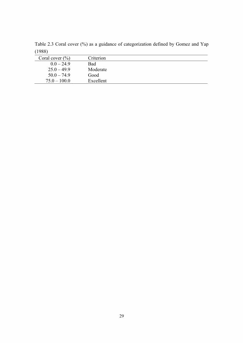
29
Table 2.3 Coral cover (%) as a guidance of categorization defined by Gomez and Yap
(1988) Coral cover (%) Criterion
0.0 – 24.9 Bad 25.0 – 49.9 Moderate 50.0 – 74.9 Good
75.0 – 100.0 Excellent
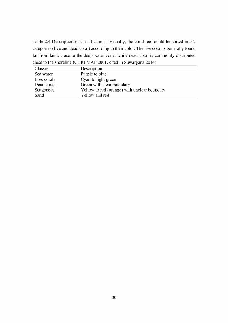
30
Table 2.4 Description of classifications. Visually, the coral reef could be sorted into 2
categories (live and dead coral) according to their color. The live coral is generally found
far from land, close to the deep water zone, while dead coral is commonly distributed
close to the shoreline (COREMAP 2001, cited in Suwargana 2014) Classes Description Sea water Purple to blue Live corals Cyan to light green Dead corals Green with clear boundary Seagrasses Yellow to red (orange) with unclear boundary Sand Yellow and red
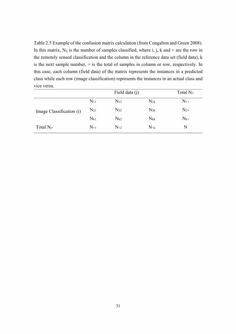
31
Table 2.5 Example of the confusion matrix calculation (from Congalton and Green 2008).
In this matrix, Nij is the number of samples classified, where i, j, k and + are the row in
the remotely sensed classification and the column in the reference data set (field data), k
is the next sample number, + is the total of samples in column or row, respectively. In
this case, each column (field data) of the matrix represents the instances in a predicted
class while each row (image classification) represents the instances in an actual class and
vice versa. Field data (j) Total Ni+
Image Classification (i)
N11 N12 N1k N1+
N21 N22 N2k N2+
Nk1 Nk2 Nkk Nk+
Total Nj+ N+1 N+2 N+k N
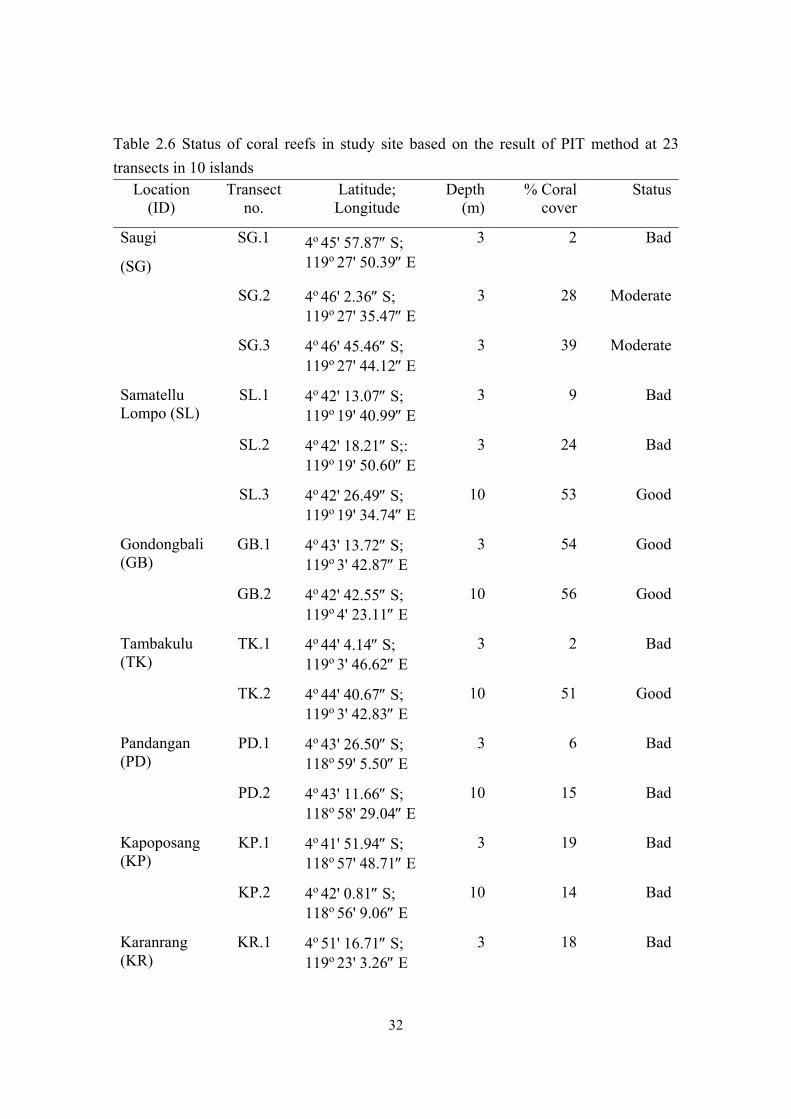
32
Table 2.6 Status of coral reefs in study site based on the result of PIT method at 23
transects in 10 islands Location
(ID) Transect
no. Latitude; Longitude
Depth (m)
% Coral cover
Status
Saugi
(SG)
SG.1 4o 45' 57.87 S; 119o 27' 50.39 E
3 2 Bad
SG.2 4o 46' 2.36 S; 119o 27' 35.47 E
3 28 Moderate
SG.3 4o 46' 45.46 S; 119o 27' 44.12 E
3 39 Moderate
Samatellu Lompo (SL)
SL.1 4o 42' 13.07 S; 119o 19' 40.99 E
3 9 Bad
SL.2 4o 42' 18.21 S;: 119o 19' 50.60 E
3 24 Bad
SL.3 4o 42' 26.49 S; 119o 19' 34.74 E
10 53 Good
Gondongbali (GB)
GB.1 4o 43' 13.72 S; 119o 3' 42.87 E
3 54 Good
GB.2 4o 42' 42.55 S; 119o 4' 23.11 E
10 56 Good
Tambakulu (TK)
TK.1 4o 44' 4.14 S; 119o 3' 46.62 E
3 2 Bad
TK.2 4o 44' 40.67 S; 119o 3' 42.83 E
10 51 Good
Pandangan (PD)
PD.1 4o 43' 26.50 S; 118o 59' 5.50 E
3 6 Bad
PD.2 4o 43' 11.66 S; 118o 58' 29.04 E
10 15 Bad
Kapoposang (KP)
KP.1 4o 41' 51.94 S; 118o 57' 48.71 E
3 19 Bad
KP.2 4o 42' 0.81 S; 118o 56' 9.06 E
10 14 Bad
Karanrang (KR)
KR.1 4o 51' 16.71 S; 119o 23' 3.26 E
3 18 Bad
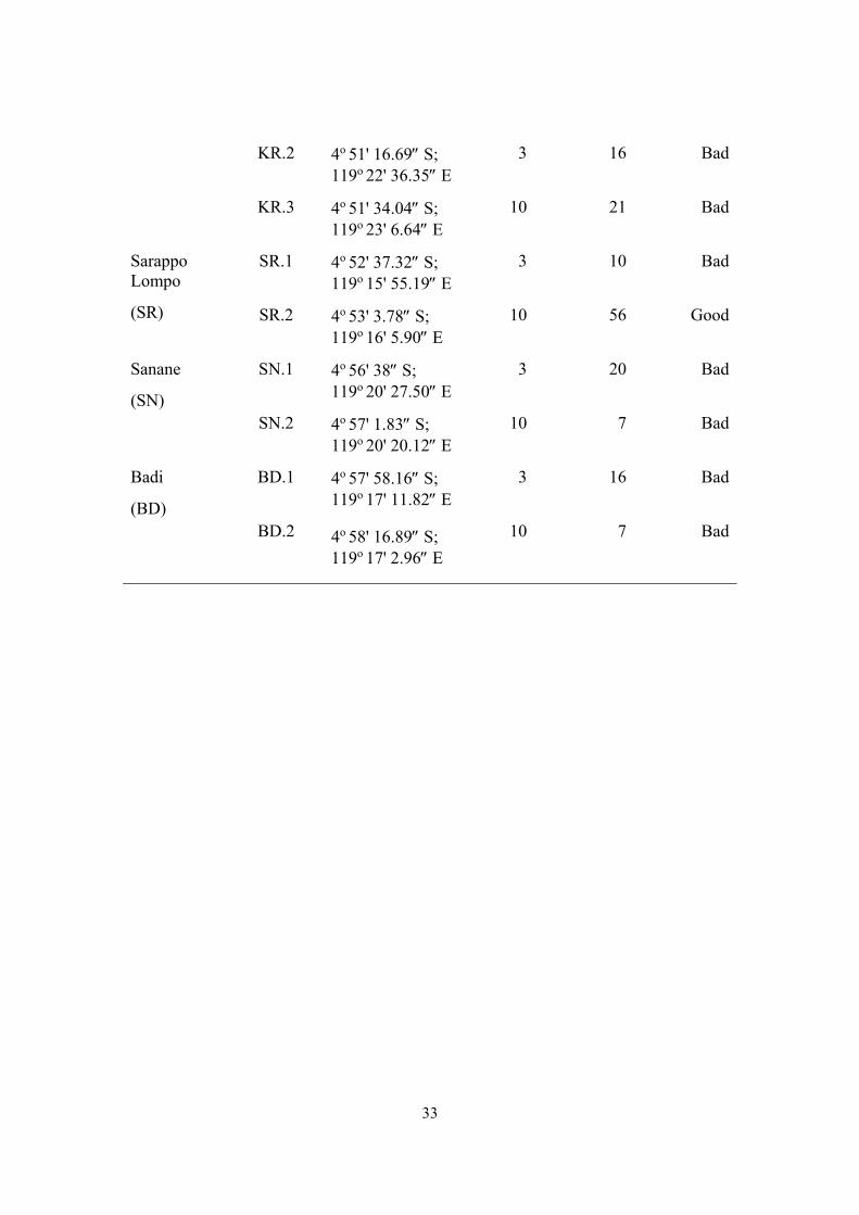
33
KR.2 4o 51' 16.69 S; 119o 22' 36.35 E
3 16 Bad
KR.3 4o 51' 34.04 S; 119o 23' 6.64 E
10 21 Bad
Sarappo Lompo
(SR)
SR.1 4o 52' 37.32 S; 119o 15' 55.19 E
3 10 Bad
SR.2 4o 53' 3.78 S; 119o 16' 5.90 E
10 56 Good
Sanane
(SN)
SN.1 4o 56' 38 S; 119o 20' 27.50 E
3 20 Bad
SN.2 4o 57' 1.83 S; 119o 20' 20.12 E
10 7 Bad
Badi
(BD)
BD.1 4o 57' 58.16 S; 119o 17' 11.82 E
3 16 Bad
BD.2
4o 58' 16.89 S; 119o 17' 2.96 E
10 7 Bad
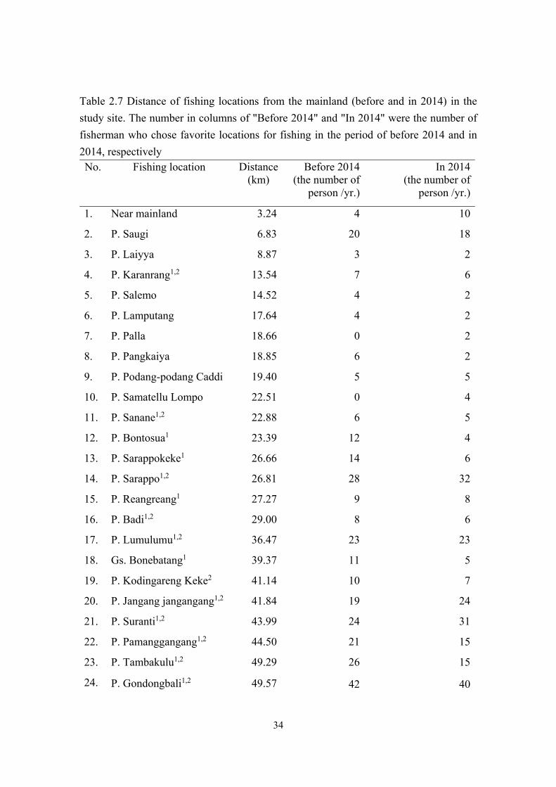
34
Table 2.7 Distance of fishing locations from the mainland (before and in 2014) in the
study site. The number in columns of "Before 2014" and "In 2014" were the number of
fisherman who chose favorite locations for fishing in the period of before 2014 and in
2014, respectively No. Fishing location Distance
(km) Before 2014
(the number of person /yr.)
In 2014 (the number of
person /yr.)
1. Near mainland 3.24 4 10
2. P. Saugi 6.83 20 18
3. P. Laiyya 8.87 3 2
4. P. Karanrang1,2 13.54 7 6
5. P. Salemo 14.52 4 2
6. P. Lamputang 17.64 4 2
7. P. Palla 18.66 0 2
8. P. Pangkaiya 18.85 6 2
9. P. Podang-podang Caddi 19.40 5 5
10. P. Samatellu Lompo 22.51 0 4
11. P. Sanane1,2 22.88 6 5
12. P. Bontosua1 23.39 12 4
13. P. Sarappokeke1 26.66 14 6
14. P. Sarappo1,2 26.81 28 32
15. P. Reangreang1 27.27 9 8
16. P. Badi1,2 29.00 8 6
17. P. Lumulumu1,2 36.47 23 23
18. Gs. Bonebatang1 39.37 11 5
19. P. Kodingareng Keke2 41.14 10 7
20. P. Jangang jangangang1,2 41.84 19 24
21. P. Suranti1,2 43.99 24 31
22. P. Pamanggangang1,2 44.50 21 15
23. P. Tambakulu1,2 49.29 26 15
24. P. Gondongbali1,2 49.57 42 40
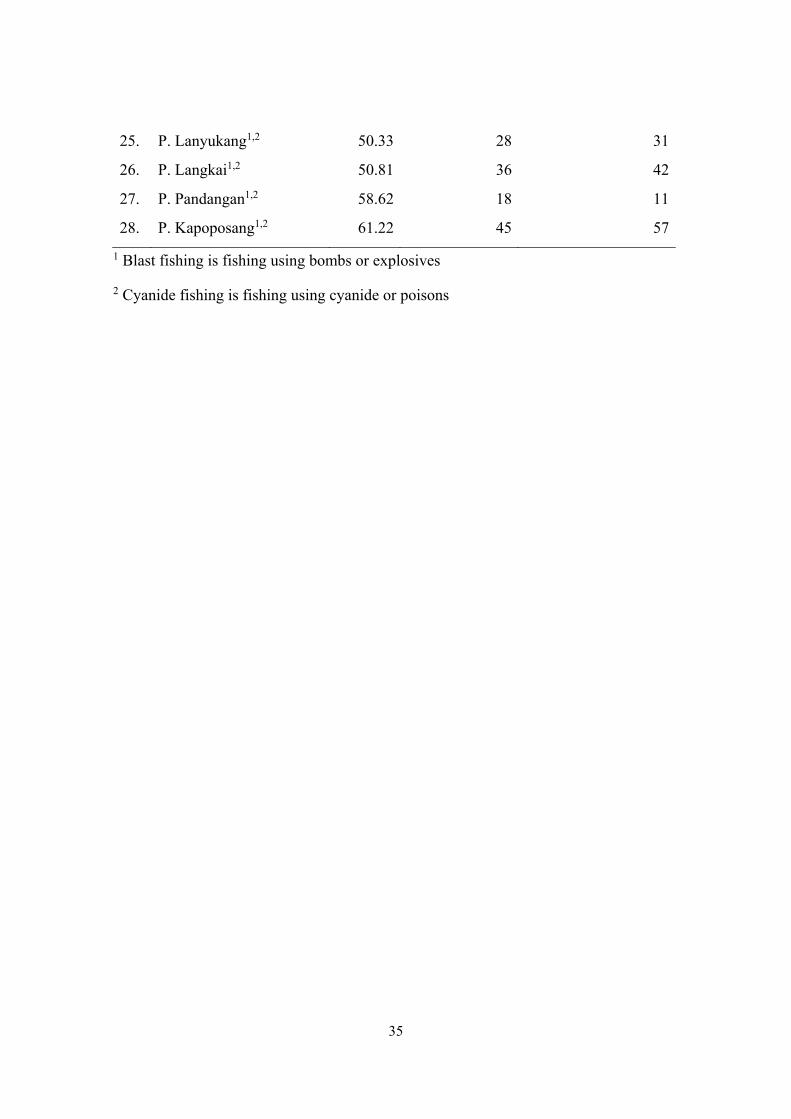
35
25. P. Lanyukang1,2 50.33 28 31
26. P. Langkai1,2 50.81 36 42
27. P. Pandangan1,2 58.62 18 11
28. P. Kapoposang1,2 61.22 45 57
1 Blast fishing is fishing using bombs or explosives
2 Cyanide fishing is fishing using cyanide or poisons
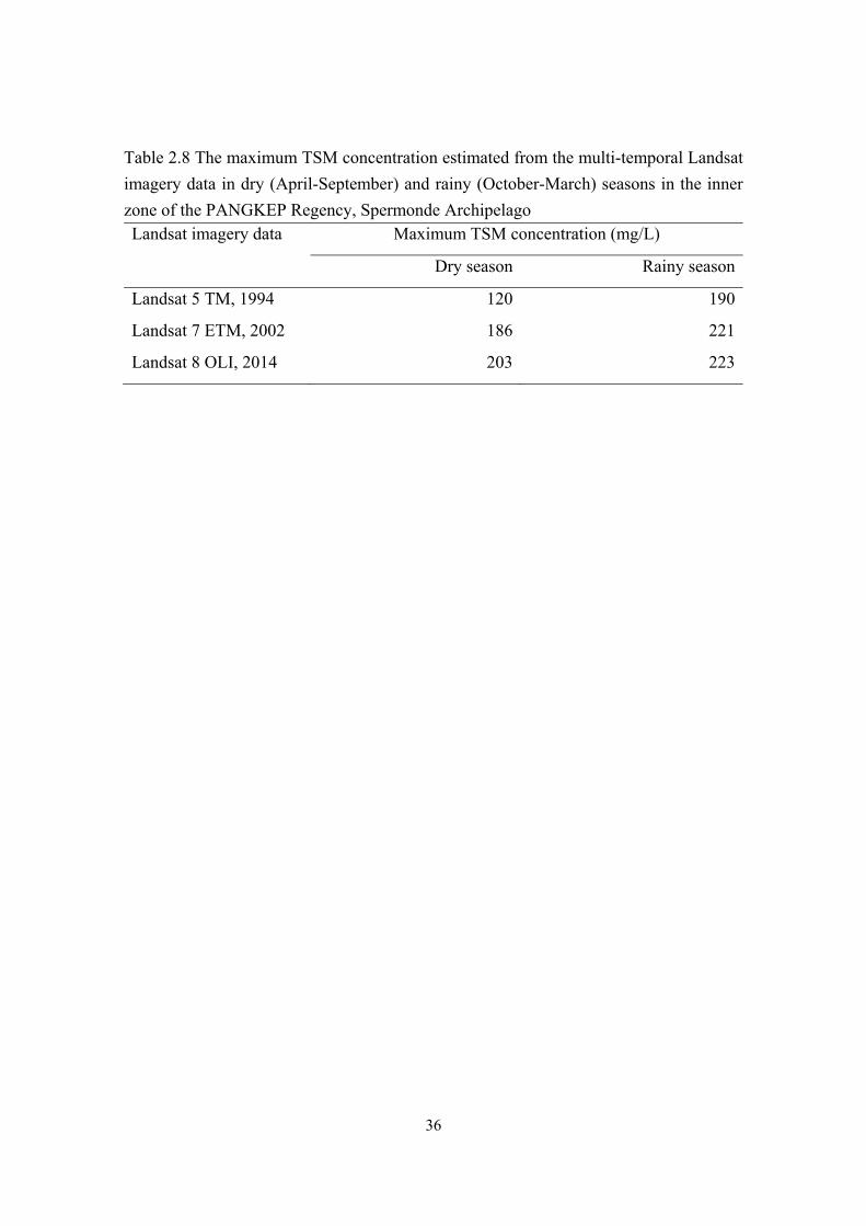
36
Table 2.8 The maximum TSM concentration estimated from the multi-temporal Landsat
imagery data in dry (April-September) and rainy (October-March) seasons in the inner
zone of the PANGKEP Regency, Spermonde Archipelago Landsat imagery data
Maximum TSM concentration (mg/L)
Dry season Rainy season
Landsat 5 TM, 1994 120 190
Landsat 7 ETM, 2002 186 221
Landsat 8 OLI, 2014 203 223

37
Table 2.9 Results of the classification of coral reefs and seabed habitats estimated by the
multi-temporal Landsat imagery data in the PANGKEP Regency, Spermonde
Archipelago, Indonesia Class Landsat 5 TM, 1994 Landsat 7 ETM, 2002 Landsat 8 OLI, 2014
Area (ha) Amount of pixel
Ratio (%)
Area (ha) Amount of pixel
Ratio (%)
Area (ha) Amount of pixel
Ratio (%)
Live corals 7,715.67 85,729 71.7 6,885.14 76,501 64.0 4,236.31 47,071 39.4
Dead corals 1,128.17 12,535 10.5 2,210.04 24,556 20.5 4,316.30 47,958 40.1
Seagrasses 655.89 7,287 6.1 846.09 9,400 7.9 906.08 10,067 8.4
Sand 1,264.86 14,054 11.8 823.32 9,148 7.7 1,305.90 14,510 12.1
Total 10,764.59 119,605 100.0 10,764.59 119,605 100.0 10,764.59 119,605 100.0

38
Table 2.10 Confusion matrix value on the classification of four classes of the seabed
habitats in the PANGKEP Regency, Spermonde Archipelago, Indonesia
Field data Field data
Row totalLive corals Dead corals Seagrasses Sand
Live corals 52 8 0 4 64
Dead corals 9 58 0 2 69
Seagrasses 2 0 40 8 50
Sand 3 0 9 48 60
Column total 66 66 49 62 243

39
Table 2.11 Ratio of producer's accuracy (PA) and the user's accuracy (UA). The
calculation was conducted for four marine habitat classifications in the PANGKEP
Regency, Spermonde Archipelago, Indonesia. Reference data mean the classes which are
classified correctl
Classification
Reference data Imagery data
The total
number of
correct pixels
The total number
of pixels in the field data
Accuracy (%)
The total
number of
correct pixels
The total number of
pixels in the image
classification
Accuracy (%)
Live corals 52 66 79 52 64 81
Dead corals 58 66 88 58 69 84
Seagrasses 40 49 82 40 50 80
Sand 48 62 77 48 60 80
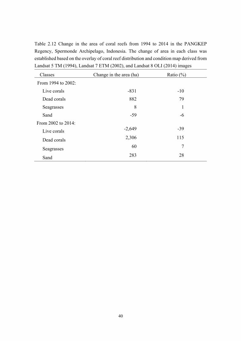
40
Table 2.12 Change in the area of coral reefs from 1994 to 2014 in the PANGKEP
Regency, Spermonde Archipelago, Indonesia. The change of area in each class was
established based on the overlay of coral reef distribution and condition map derived from
Landsat 5 TM (1994), Landsat 7 ETM (2002), and Landsat 8 OLI (2014) images
Classes Change in the area (ha) Ratio (%)
From 1994 to 2002:
Live corals -831 -10
Dead corals 882 79
Seagrasses 8 1
Sand -59 -6
From 2002 to 2014:
Live corals -2,649 -39
Dead corals 2,306 115
Seagrasses 60 7
Sand 283 28

41
Figure 2.1 Categories used in PIT method. AC: Acropora; NA: Non-Acropora; SP:
Sponge; R: Rubble; SC: Soft coral; SA: Sand; DCA: Dead coral algae; A: Abiotic. In
this case, the rubble was classified as dead corals
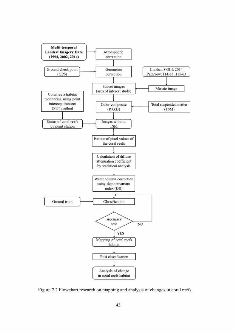
42
Figure 2.2 Flowchart research on mapping and analysis of changes in coral reefs
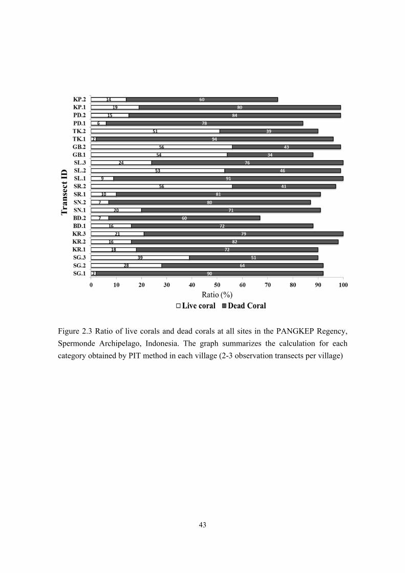
43
Figure 2.3 Ratio of live corals and dead corals at all sites in the PANGKEP Regency,
Spermonde Archipelago, Indonesia. The graph summarizes the calculation for each
category obtained by PIT method in each village (2-3 observation transects per village)
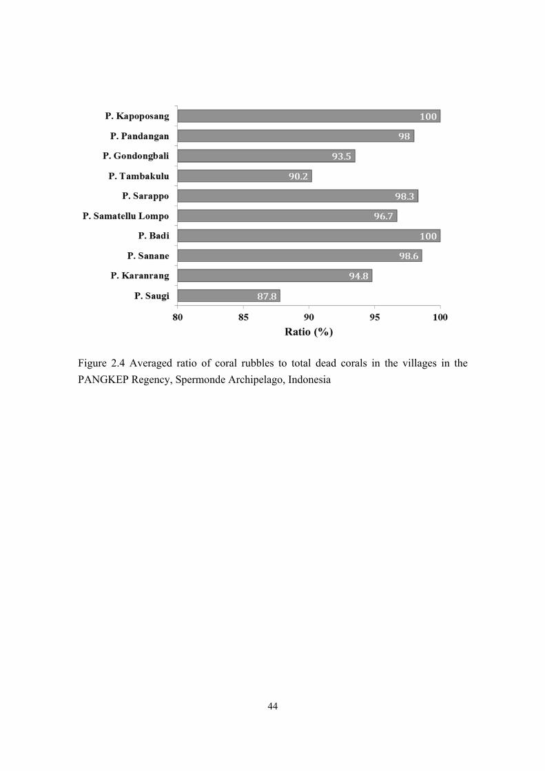
44
Figure 2.4 Averaged ratio of coral rubbles to total dead corals in the villages in the
PANGKEP Regency, Spermonde Archipelago, Indonesia
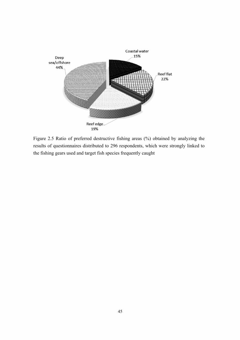
45
Figure 2.5 Ratio of preferred destructive fishing areas (%) obtained by analyzing the
results of questionnaires distributed to 296 respondents, which were strongly linked to
the fishing gears used and target fish species frequently caught
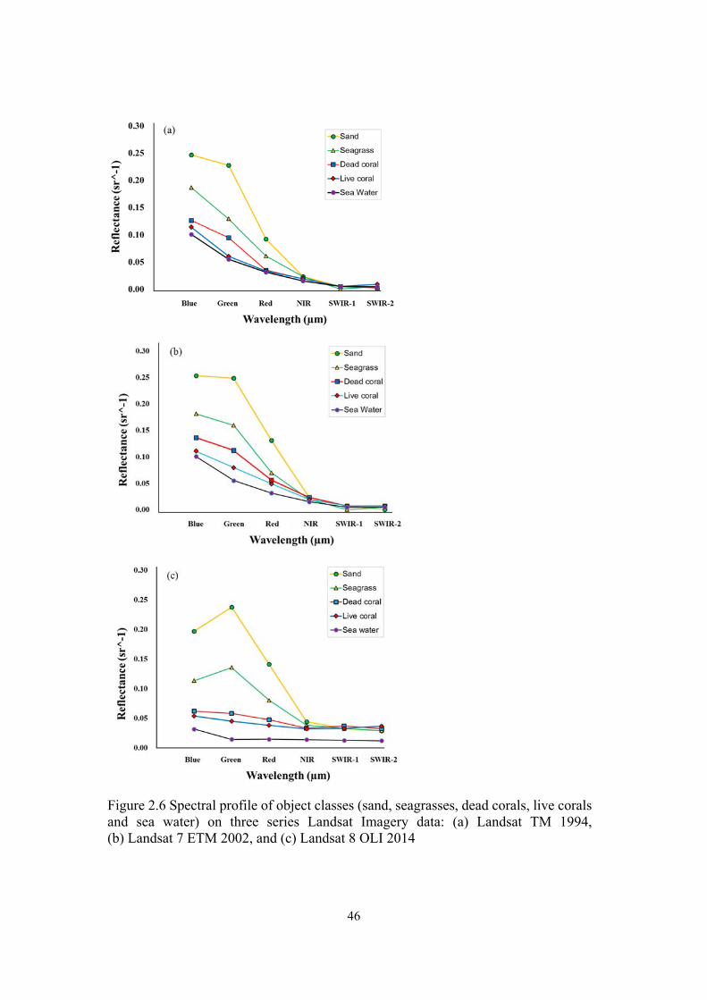
46
Figure 2.6 Spectral profile of object classes (sand, seagrasses, dead corals, live corals and sea water) on three series Landsat Imagery data: (a) Landsat TM 1994, (b) Landsat 7 ETM 2002, and (c) Landsat 8 OLI 2014
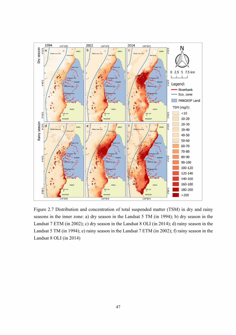
47
Figure 2.7 Distribution and concentration of total suspended matter (TSM) in dry and rainy
seasons in the inner zone: a) dry season in the Landsat 5 TM (in 1994); b) dry season in the
Landsat 7 ETM (in 2002); c) dry season in the Landsat 8 OLI (in 2014); d) rainy season in the
Landsat 5 TM (in 1994); e) rainy season in the Landsat 7 ETM (in 2002); f) rainy season in the
Landsat 8 OLI (in 2014)
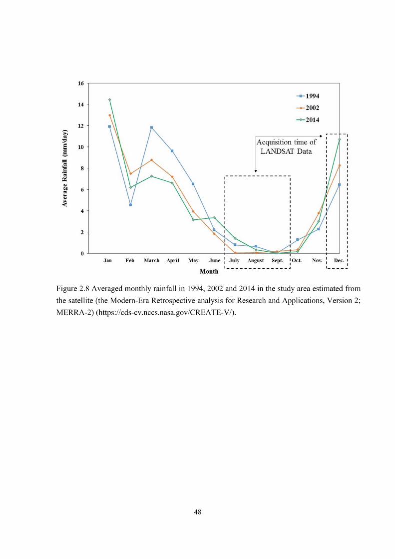
48
Figure 2.8 Averaged monthly rainfall in 1994, 2002 and 2014 in the study area estimated from
the satellite (the Modern-Era Retrospective analysis for Research and Applications, Version 2;
MERRA-2) (https://cds-cv.nccs.nasa.gov/CREATE-V/).
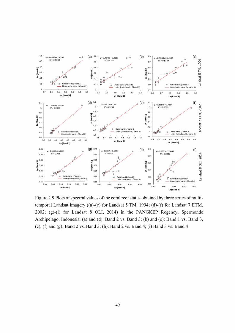
49
Figure 2.9 Plots of spectral values of the coral reef status obtained by three series of multi-
temporal Landsat imagery ((a)-(c) for Landsat 5 TM, 1994; (d)-(f) for Landsat 7 ETM,
2002; (g)-(i) for Landsat 8 OLI, 2014) in the PANGKEP Regency, Spermonde
Archipelago, Indonesia. (a) and (d): Band 2 vs. Band 3; (b) and (e): Band 1 vs. Band 3,
(c), (f) and (g): Band 2 vs. Band 3; (h): Band 2 vs. Band 4; (i) Band 3 vs. Band 4

50
Figure 2.10 Depth invariant index derived from three series of multi-temporal
Landsat imagery data ((a)-(c) for Landsat 5 TM, 1994; (d)-(f) for Landsat 7 ETM,
2002; (g)-(i) for Landsat 8 OLI, 2014) in the PANGKEP Regency, Spermonde
Archipelago, Indonesia, using gradient of the linier line. (a) and (d): Band 2 vs. Band
3; (b) and (e): Band 1 vs. Band 3, (c), (f) and (g): Band 2 vs. Band 3; (h): Band 2 vs.
Band 4; (i) Band 3 vs. Band 4
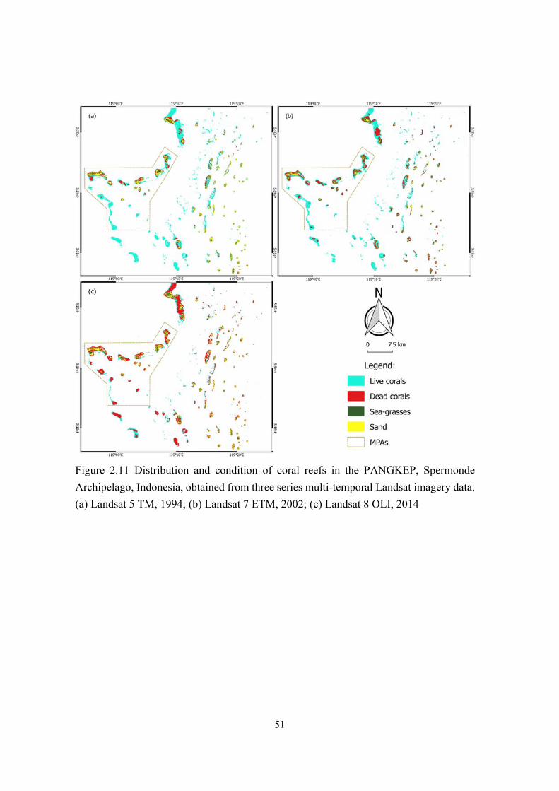
51
Figure 2.11 Distribution and condition of coral reefs in the PANGKEP, Spermonde
Archipelago, Indonesia, obtained from three series multi-temporal Landsat imagery data.
(a) Landsat 5 TM, 1994; (b) Landsat 7 ETM, 2002; (c) Landsat 8 OLI, 2014

52
Figure 2.12 Map of change in bottom substrate in the PANGKEP Regency,
Spermonde Archipelago, Indonesia: (a) from 1994 to 2002 and (b) from 2002 to
2014. The Kapoposang MPAs is located in the outer zone of the PANGKEP islands
which also experienced a drastic decline in coral reef habitats in this period

53
Figure 2.13 Change in composition of coral reefs from 1994 to 2014. During the period,
45.1% of the coral reef area has been transformed (left pie chart): 91.6% from live to dead
corals, 7.2% from live corals to sand, and 1.2% from dead corals to sand (right pie chart)

54
Figure 2.14 Tidal prediction in the PANGKEP Regency, Spermonde Archipelago,
Indonesia with a coordinate point of observation: 1190 15'36 S and 40 48'36 E. The data
is processed by using the prediction model from
http://www.miz.nao.ac.jp/staffs/nao99/index_En.html. Accessed 10 October 2016

55
Chapter III Economic assessment of the benefits and losses of goods and services
derived from coral reefs: a case study in the Pangkajene and Kepulauan Regency, Spermonde Archipelago, Indonesia
3.1 Introduction Coral reefs are among the most productive ecosystems in the marine environment,
and have functional roles in supplying goods and services for human benefits, including
fisheries, tourism, scientific research, shoreline protection, and medicines (e.g., Moberg
and Folke 1999; Souter and Linden 2000; UNEP 2006; Brander et al. 2007; Tseng et al.
2015). Regrettably, coral reef ecosystems are severely threatened and many are in a
devastated condition, either due to negative impacts associated with human activities (e.g.,
destructive fishing practices, reclamation, pollution, waste dumping, and uncontrolled
tourism activities) or the effects of climate change (e.g., ocean acidification, bleaching
phenomena, and sea-level rise) (Morton 1994; McManus et al. 1997; Pet-Soede 2000;
Harley et al. 2006; Brander et al. 2007; Burke et al. 2011; Yusuf and Jompa 2012; Nashr
2015; Pendleton et al. 2016). In addition, nutrient runoff from soil erosion and fertilizers
are potentially serious threats to the long-term sustainability of coral reef ecosystems,
causing outbreaks of crown-of-thorns starfish (Wooldridge and Brodie 2015; Lamy et al.
2016) and coral reef diseases due to certain pathogenic viruses that infect coral reefs (Weil
et al. 2006; Haapkyla et al. 2011). The destruction and loss of coral reefs result in a
significant ecological imbalance of the marine environment in the form of dynamic,
structural, and functional changes to ecosystems, especially the abundance and
biodiversity of coral fish and loss of fish species that rely on coral reef ecosystems
(Hughes 1995; Weil et al. 2006; Komyakova et al. 2013). This leads to a reduction in the
economic value of coral reefs in terms of supplying goods and services for the benefit of
human society.
The factors influencing the destruction of coral reefs mentioned above have
affected the condition of coral reefs in the Pangkajene and Kepulauan (PANGKEP)
Regency, Spermonde Archipelago, Indonesia, which was the study location selected for
this study (Figure 1.1). Several previous studies have indicated that coral reefs in this area
are in a seriously bad condition. The Coral Reef Rehabilitation and Management Program
(COREMAP) in 2005 founded that 74.26% of the coral reefs in the PANGKEP Regency
were in a bad condition, and only 25.74% of them were in good condition
(http://kkji.kp3k.kkp.go.id/index.php/en/marine-protected-area-data/details/7/92). The
dominant causal factors of the destruction of coral reefs in the study area are destructive

56
fishing practices, collecting coral for use as a building material, and coral bleaching that
has occurred from the end of 2009 until mid-2010, accounting for approximately 12% of
the total coral reef damage (Yusuf and Jompa 2012).
Using multi-temporal LANDSAT images, Yasir Haya and Fujii (2017) estimated
that live coral cover had been reduced from 7,716 ha in 1994 to 6,885 ha in 2002, and to
4,236 ha in 2014, or by 174 ha/yr during the period from 1994 to 2014. The study was
based on the calculation of the percentage cover of both live coral and coral rubble using
the point intercept transect (PIT) method in the vicinity of 10 islands in the PANGKEP
Regency, Spermonde Archipelago. They concluded that live coral cover was present in
only 24% of the study area, while 95.8% of the area contained some dead coral in the
form of rubble spread across various sites, suggesting that the majority of coral damage
was caused by destructive fishing practices, namely blast fishing, cyanide fishing, and the
use of mini trawl nets (DFW-Indonesia 2003; Chozin 2008; Nurdin and Grydehoj 2014).
Destructive fishing activities have large-scale destructive impacts, not only in
terms of damage to coral reefs but also due to loss of biological productivity and economic
benefits, i.e., reef fisheries, marine tourism, coastal protection (White et al. 2000; Wells
2009), and the livelihood of fishermen. This has even triggered social conflicts among
coastal communities (DFW-Indonesia 2003; Nurdin and Grydehoj 2014). The high
intensity of destructive fishing activities can result in the functional disturbance of coral
reefs as a supply of goods and services for the benefit of human society. Such disturbances
can reduce the income of local people, which leads to a reduction in the utilization of
coral reefs (Grigalunas and Congar 1995; Moberg and Folke 1999).
From an economic perspective, coral reef destruction leads to a loss of economic
value of coral reefs and has long-term economic impacts. Healthy reefs contribute
approximately 20 tons/km2/yr of fish and edible products, but the destruction of coral
reefs due to dynamite and cyanide fishing reduces the production of fish by approximately
4 tons/km2/yr (White et al. 2000). The damage caused to coral reefs results in an estimated
average economic loss of between 33,900 and 306,800 USD/km2 (Pet-Soede et al. 1999).
In Indonesia, the use values (UVs) of coral reefs, i.e., its contribution to the economic
benefits of the fisheries sector, tourism sector, and coastal protection are 2.2 billion, 258
million, and 782 million USD/km2/yr, respectively (Burke et al. 2011). Those economic
values do not include the value of biodiversity, the value of bequeathing coral reefs, and
the value of their continued existence.
The aim of this study was to determine the economic benefits of coral reef
ecosystems and to calculate the economic losses due to coral reef damage. The economic
benefits of coral reefs estimated in this study refer to the economic value typology in the

57
framework of the total economic value (TEV) formulated by Pagiola et al. (2004), Pierce
and Morgan (2009), and Freeman III et al. (2014). The TEV is measured by the UVs of
ecosystem goods and services: the direct use value (DUV), indirect use value (IUV), and
non-use value (NUV) (i.e., the value of bequeathing coral reefs and the value of their
continued existence). In addition, economic losses due to the degradation of coral reefs
were estimated.
It is expected that the estimation of both the benefits and losses associated with
coral reefs in this study could be used as a recommendation for policy makers when
allocating the UVs of coral reefs, and as a reference for sustainable coral reef management.
The valuation (i.e., the monetary price) of the coral reef economy could also be used as
input data by public administrators and stakeholders to determine the compensation
required due to coral reef destruction, which can occur at any time due to certain
destructive ecological activities (Grigalunas and Congar 1995; Boyd 2010).
3.2 Materials and Methods 3.2.1 Data source and materials
3.1.1.1 Data source
The study used both primary and secondary data. The primary data were collected
from questionnaires and direct interviews, whereas the secondary data were gathered
from statistical data, existing documentation, and previous research reports published by
several formal institutions, i.e., fisheries statistical data, visitation data (tourists and
researchers), and data relating to the cost of coastal protection (Saunders et al. 2007). The
respondents interviewed to obtain the UVs of reef-related fisheries were traditional
fishermen, commercial fishermen, and seaweed farmers, and were all inhabitants of the
selected islands.
A purposive random sampling method was used, in which the local fishermen
were classified into two categories according to the fishing gear and fisheries production
(Sekaran 2003), with a minimum sample size of 30 for each group (Sekaran 2003; Howell
2016). The respondents interviewed to obtain the UVs of reef-related tourism and
scientific research were dive operators, university lecturers/students, officials from the
marine and fisheries agency of PANGKEP Regency, and residents from the local
communities.
3.1.1.2 Questionnaire survey
A questionnaire was designed to obtain data and information related to fisheries,
tourism, research, and the respondents' perspective regarding the value of reef ecosystems
58
(Appendix A1). The questionnaire collected selected personal details of those surveyed
(i.e., name, age, education level, selling price of fish, income level, and the number of
family members), the type of fishing gear used, fishing locations, operational costs, and
the willingness to pay (WTP) for the continued existence of coral reefs.
3.2.2 Framework valuation of the total economic value
One approach to evaluate the economic benefits of coral reef ecosystems is the
total economic value (TEV) (Pagiola et al. 2004; Pearce and Moran 2009; Freeman III et
al. 2014):
TEV = UV + NUV = (DUV + NUV) + (BV+ EV), (3.1)
where UV is the use value (USD/yr), NUV is the non-use value (USD/yr), DUV is the
direct use value (USD/yr), NUV is the non-direct use value (USD/yr), BV is the bequest
value (USD/yr), and EV is the existence value (USD/yr).
The derivative equations of the total economic value (TEV) of coral reef
ecosystems are presented in the following subsections.
3.2.2.1 DUVs of coral reefs
DUVs of coral reef ecosystems in this study were a consequence of use by the
fisheries, tourism, and scientific research sectors. The equation used to calculate the value
is written as follows (Fauzi 2006):
, (3.2)
where DUV is the total direct use value (USD/yr) and Qi is the DUV of the individual
sectors.
Here, Q1 is the DUV of reef-related fisheries (USD/yr), Q2 is the DUV of reef-
related tourism (USD/yr), and Q3 is the DUV of reef-related scientific research (USD/yr).
a. DUVs of reef-related fisheries
DUVs of coral reefs from the fisheries sector were derived from catching fish and
seaweed farming. Coral fishes, crabs, squids and octopuses, and seaweeds all contribute
to the value of reef-related fisheries, which was estimated using the effect on production
(EOP) method, based on a production approach (Grigalunas and Congar 1995; Chee
59
2004; Adrianto 2006). The calculation of DUVs for reef-related fisheries involves several
steps (Adrianto 2006; Wahyuddin 2007; Wawo et al. 2014) as follows:
1) Determine the demand function for a given resource, which includes coral fishes,
crabs, squids, octopuses, and seaweed farming, using the following demand
equation (3.3) (Appendix A2):
Q = β V1 a V2
b V3 cV4
d, (3.3)
where Q is the total resource gained, V1 is the market price per unit of resource
calculated in all sites of the study, whereas V2, V3, and V4 are variables regarding
the socio-economic status of respondents or users of reef-related resources, β is the
intercept, a is the coefficient of the price, whereas b, c, and d are coefficients of
the socio-economic status of respondents or users of reef related resources.
2) Linear transformation of the demand function Q to obtain the coefficient value of
each selected parameter using a linear regression, as shown in Appendix A2.
3) Approach the tabulated result with a linear regression.
4) Obtain the total WTP and consumer surplus (CS) using Maple software. Maple is
a math software that combines the world's most powerful math engine with an
interface that makes it extremely easy to analyze, explore, visualize, and solve
mathematical problems (Maple 2015).
5) Calculate the area’s economic value in terms of utilization activities by
multiplying the CS with the number of fishermen/farmers.
6) Obtain the utilization economic value per ha by dividing the area’s economic
value by the total area of live coral cover.
The calculations used in procedures 2) to 5) are given in detail in Appendix A2.
b. DUVs of reef-related tourism and scientific research
The DUVs of coral reefs related to tourism and scientific research were estimated
using the travel cost (TC) method (Sinden 1994; Chee 2004). In this approach, the average
cost spent by each person to take trips and receive benefits from coral reef ecosystem at
certain tourism and research locations were calculated. The tourism related cost was
estimated and converted to an economic value, which consisted of a transportation fee,
lodging tariff, food and beverage charges, equipment rental, and an entrance ticket. The
annual DUVs of reef-related tourism were obtained by multiplying the average cost per
trip with the total number of visitors (tourists) per year. The method used in this study to
60
estimate the DUVs of reef-related tourism was the TC method, which was also applied to
determine the DUVs for reef-related research activities.
3.2.2.2 IUVs of coral reefs
IUVs are indirect benefits gained from coral reef ecosystems, i.e., coastal
protection, and biological support to fisheries, turtles, and other marine life. In this study,
the benefit of coral reefs as a natural form of coastal protection was examined.
An estimation of the benefits of coral reefs as a natural form of coastal protection
was made using the replacement cost (RC) method, by calculating the construction costs
of breakwaters along the shorelines of 31 inhabited islands. Unit costs and volumes for
the breakwater construction were obtained from the Regional Department of Public
Works of the PANGKEP Regency.
The calculation of IUVs of reef-related coastal protection consists of two steps as
follows.
First, the volume of the breakwater (V (m3)) was calculated as follows:
V L W H , (3.4)
where LS is the coastline length (m), WB is the barrier width (m), and HB is the barrier
height (m).
Second, the coastal protection value of coral reefs (SPV (USD)) was calculated
by multiplying the volume of breakwaters (V) with the construction cost per unit (C,
USD/m3) as follows:
SPV V C, (3.5)
3.2.2.3 NUVs of coral reefs
NUVs are the values of coral reefs that people assign to economic goods
(including public goods) even if they never have and never will use them. They can be
distinguished from the UVs, which are derived from the direct use of the goods. The
NUVs estimated in this study were the value of bequeathing coral reefs and the value of
their continued existence.
a. Bequest Values (BVs)
BVs are benefit values given by individuals based on their WTP to save coral reef
resources to make them available for future generations. In this case, this study was used

61
the benefit transfer (BT) method to estimate the BV. This was based on Hargreaves-Allan
(2004) who estimated the bequest values of coral reefs off Wakatobi Island, Indonesia,
which is close to the study area. The BV of coral reefs is 412,000 USD/ha/yr (2004). In
this case, the Hargreaves-Allen’s value in 2004 was adjusted for inflation to obtain the
correct value for 2014 using the following equation (Unsworth and Peterson 1995):
,
(3.6)
where BV(Yi) and GDP(Yi) are the BV and gross domestic product (GDP) in Indonesia
(Organization for Economic Co-operation and Development (OECD), 2016), and BVHA
is the Hargreaves-Allen’s BV from 2004 (i.e., 412,000 USD/ha/yr).
In addition, the value of BV(Yi) was used to estimate the BV in the study area
using the BT method.
b. Existence Values (EVs)
When consmers’s preferences are not revealed by markets, economists usually
use direct questions regarding their WTP for services or goods to calculate their
preferences. One of the approaches most often used is the contingent valuation method
(CVM), which is favored by researchers due to its applicability to a variety of
environmental goods and its capacity to assess the EV (Aoun 2015). The EV is the value
obtained solely due to the presence of natural resources and the environment. The EVs of
coral reefs were estimated based on individuals’ WTP for coral reef resources (FAO
2000). The WTP data among the respondents in this study were obtained by questionnaire
and direct interviews. The EVs were calculated based on Wahyudin (2007) using the
follows steps:
1) Determination of the WTP function for the NUVs of coral reefs using the following
equation:
WTP = β0 X1 β1 X2
β2 X3 β3 …Xn βn, (3.7)
where X1, X2, X3…Xn are the variables of economic and social status among individuals
or users of reef-related resources. β0 is the intercept, whereas β1, β2, β3…βn are the
coefficients of socio-economic status of respondents or users of reef related resources.

62
2) Transformation of the WTP function into a linear function to estimate each of the
parameters analyzed using linear regression. Equation (3.7) is then transformed into
the following equation:
ln WTP = β0 + β1 lnX1 + β2 ln X2 + β3 lnX3 + … βn ln Xn,
= {β0 + β1 ln 1 + β2 ln 2 + β3 ln 3 + … βn ln n},
= β’, (3.8)
where 1, 1, 3 … are the average natural logarithm of the education level,
income, age, family member and other social factors, and β’ is the sum of the
coefficient intercept added to the average of the natural logarithm of each variable
multiplied by the coefficient of each variable.
3) Equation (3.8) was then back transformed to its original function to calculate the value
of the WTP per capita, using the following equation:
WTP = exp (β’), (3.9)
4) Calculation of the EVs of coral reef ecosystems in a certain location (i.e., PANGKEP
Regency) by multiplying the WTP values with total users (N) of the reef-related
resource using the following equation:
EV = WTP × N, (3.10)
5) Calculation of coral reef EV per ha (EVHA) (USD/ha) by dividing the EV by the
coral reef area (L; ha) for a certain location (i.e., PANGKEP Regency), using the
following equation:
EVHA = . (3.11)
3.2.3 Economic losses of coral reef destruction
The overexploitation of natural resources has a negative impact on ecology and
biodiversity. Economic activities may damage ecosystem functions and, subsequently,
ecosystem services that lead to human wellbeing and balanced ecosystems (Grigalunas
and Congar 1995; Moberg and Folke 1999; Chapin et al. 2000). The economic losses due
to coral reef destruction were estimated with the following assumptions: (1) the only
63
changeable variable was coral reef area (3,480 ha degraded during the period of 1994 –
2014 or a destruction rate of 174 ha/yr (Yasir-Haya and Fujii 2017); (2) the component
of coral reef values used to estimate the economic losses was the UV; (3) the local
currency (Indonesian Rupiah; IDR) was converted into USD (1 USD = IDR 13,000).
To discount the economic losses from past coral reef degradation, it was
determined whether the discounted values were expressed in real or nominal terms. Real
values have been adjusted for inflation, while nominal values are expressed in uninflated
terms. This approach was proposed by the Division of Economics, U.S. Fish, and Wildlife
Service, to assess the resulting damage due to the release of oil or other hazardous
materials to the environment (Unsworth and Peterson 1995). This approach can be used
to estimate the current value of the economic loss due to coral reef damage in the study
area. To obtain these values in real terms, the inflation rate from 1994 to 2014 was
adjusted. Using the GDP Implicit Price Deflator (Brander et al. 2007), the value of
economic loss due to past coral reef damage was determined using the following formula
(Unsworth and Peterson 1995):
where is the present value of the economic loss in year i (value in USD) and
is the economic loss in year i (value in USD).
Furthermore, to obtain the total economic loss (TEL) from 1994 to 2014, real
discount rates were calculated using the following formula:
1 . (3.13)
where TEL1994-2014 is the TEL from 1994 to 2014 and r is the discount factor.
In this case, this study was set the discount rate to 10% (White et al. 2000; Cesar
2002) to obtain the current value of coral reef damage or economic loss.
3.3 Results and Discussion
,
(3.12)

64
3.3.1 Use values (UVs) of coral reefs
Based on the TEV framework of this study, the UVs of coral reefs consisted of
DUVs and IUVs.
3.3.1.1 Direct use values (DUVs)
Based on the field survey and the data analysis, the categories of economic
benefits included in the DUVs were set as reef related fish, crab, squid, and octopus
catches, seaweed farming, tourism, and scientific research. The results of this calculation
are presented in the following section.
a. DUV of reef-related fisheries
Based on the questionnaire results, average prices (P) varied between 1.63 and
3.05 USD/kg, whereas the education level (E) was mostly elementary school (60%) and
junior high school (40%). The age of the fishermen conducting fishing activities in the
coral reef areas varied between 41 and 48 years old, with the number of family members
ranging from 5 to 7 people. These data were processed using regression analysis to obtain
the demand function, and then processed using Maple software to determine the demand
curve (Figure 3.2), the values of the WTP, and consumer surplus (Appendix A3).
Based on the calculation, the total DUV of coral reef-related fisheries was 2.9
million USD/yr (Table 3.1). Seaweed farming accounted for most of this figure (1.3
million USD/yr), while the rest consisted of coral reef fish, crabs, squids, and octopus
(803,000, 513,000, and 251,000 USD/yr, respectively). These values indicate the
production value of the coral reef fisheries in 2014. The values obtained from demand
function were reflected in the form of a demand curve (Figure 3.1). This figure shows
that the production rate was relatively low for coral reef fish, and squid and octopuses,
both of which are sold for high prices in the market. On the other hand, crabs and
seaweeds were produced in large quantities and were sold at cheaper prices.
The total UV of coral reefs was estimated to be as low as USD 2.9 million or 675
USD/ha, with total coral reef cover of 4,236 ha in 2014 (Table 3.1). This value is much
higher than that of the Taka Bonerate Marine Protected Area (MPA), South Sulawesi,
Indonesia (7.8 USD/ha) (Sawyer 1992) and the Great Barrier Reef MPA (4.2 USD/ha)
(Driml 1999). The BV of reef fisheries (675 USD/ha) in the study area was also high
compared to the BV of reef fisheries in the Great Barrier Reef MPA (4.2 USD/ha; Driml
1999) and in the Taka Bonerate MPAs (7.8 USD/ha; Sawyer 1992). This discrepancy is
possibly caused by differences in the management systems. In MPAs, the use of coral
reefs has been regulated according to a zoning system (i.e., core zone, buffer zone, use
zone, etc.), with fishing activities only permitted in the use zone. In contrast, there is no
65
zoning system for the use of coral reefs implemented in the area investigated in this study.
Coral reef management without a zoning system tends to encourage excessive
exploitation of coral reefs by fishermen throughout the year. Therefore, effective
management of coral reefs will initially reduce the income of fishermen, but will provide
a more sustainable option in the long term. These results are consistent with the income
model proposed by Pet-Soede et al. (1999) in terms of a comparison of fishermen’s net
income when practicing either destructive or non-destructive fishing.
However, the BV of reef-related fisheries in this area is much lower than the
global average BV of reef-related fisheries (Costanza et al. 1997), which is 2.2 million
USD/ha. There are several reasons for this discrepancy, including an annual increase in
the number of local fishermen, which causes a significant loss of production value in the
coral reef fisheries. The high price of fish as a commodity in the domestic market
encourages fishermen to intensify their fishing activities, which in turn leads to
overexploitation and a loss of coral reef value. The low economic benefit regarding the
direct value of this overexploitation has resulted in massive coral reef degradation in the
region.
b. DUVs of reef-related tourism and recreation
The DUVs of coral reef-related tourism and recreation were determined by
calculating the total expenses incurred by tourists or visitors. The questionnaire results
showed that there were two main tourism destinations in the PANGKEP Regency, the
Kapoposang Marine Park and Panambungan Island. In 2014, the Kapoposang Marine
Park and Panambungan Island received 150 and 50 visitors, respectively (Statistics
Indonesia, Regency of Pangkajene and Kepulauan 2014). The average TC obtained from
the interview respondents was 723 USD/person/trip (Kapoposang Marine Park) and 154
USD/person/trip (Panambungan Island), which included fees for round-trip transportation,
accommodation, scuba diving equipment, local guides, boat rental, food and beverage
charges, and other costs (Table 3.2). Assuming an average duration of four days per trip
(Kapoposang Marine Park) and one day per trip (Panambungan Island), the DUV of reef-
related tourism and recreation in the Kapoposang Marine Park and Panambungan Island
was estimated to be USD 108,462 and USD 7,700, respectively (Table 3.3).
Hence, the total UV of reef-related tourism and recreation in the two largest
destinations in 2014 was estimated to be USD 116,162 or 27 USD/ha (Table 3.3). This
value is lower than the value reported for several similar tourist destinations, including
the Danajon’s reefs in the Philippines (227 USD /ha). According to Samonte et al. (2016),
the net benefits of coral reefs from tourism and recreation have high annual BVs if the

66
coral reefs are well managed and intact. For example, the BVs of coral reefs are estimated
to be 663 million USD/yr in the Caribbean, 269 million USD/yr in Pacific, 779 million
USD/yr in Japan, 483 million USD/yr in the USA and 1,147 million USD/yr in Australia
(Cesar et al. 2003).
Based on the responses of the interviewees, there were several factors responsible
for the small number of tourists who visited the Kapoposang Marine Park. (1)
Kapoposang Island is located in the outer zone of PANGKEP Regency and is far from
the mainland of Sulawesi, from either Makassar City or PANGKEP Regency. It requires
a 6-8 hour boat journey to reach the location. (2) There is no public transport available
for tourists and, therefore, extra fees are required to rent boats. (3) Destructive fishing
(e.g., blast and cyanide fishing) is practiced intensively at Kapoposang Island. This has
resulted in many issues with visitors who are concerned about safety. Tourists have
therefore been encouraged to visit other locations where destructive fishing is less widely
practiced.
c. DUVs of reef-related scientific research
The economic value of reef-related scientific research was also calculated using
the TC method. The total number of researchers who visited the study area in 2014 was
71 (Statistics Indonesia, Regency of the PANGKEP 2014), which included researchers,
professors, and students. The average duration of stay to conduct research in the study
area was four days, with an average cost of 231 USD/person/trip. Hence, the DUV of
reef-related scientific research was estimated to be USD 16,401 or 3.87 USD/ha in 2014.
3.3.1.2 Indirect use value (IUV)
Based on the calculated length of the coast line of the 31 inhabited islands (37,995
m), barrier width (1 m), and barrier height (1.5 m), then a volume of the coastal protection
barrier of 56,992.50 m3 was obtained. If the construction cost of the barrier was assumed
to be 297 USD/m3, then the total UV of reef-related shoreline protection was USD
16,931,157 or 3,997 USD/ha. This amount represents the economic value of coral reefs
functioning as a barrier to prevent coastal erosion.
3.3.2 Non-use values (NUVs) of coral reefs
The NUVs investigated in the PANGKEP Regency, Spermonde Archipelago,
consisted of both bequest values (BVs) and existence values (EVs), respectively. The
annual total NUV of coral reefs estimated in the study area was USD 11,949,932,130.
The estimated NUVs of coral reefs are described below.
67
3.3.2.1 Bequest Value (BV)
Using the BT method, and by adjusting to the 2004-2014 inflation rate and the
GDP Implicit Price Deflator, the BV of coral reefs in the study area was estimated to be
USD 11,947,701,429 (Table 3.3). The results clearly show that the high value in the study
area was due to the vast area of live coral cover (4,236 ha).
The high value in the study area reflects the significant public concern regarding
the current status of the coral reef ecosystem, as well as the desire to preserve the coral
reef ecosystem for future generations.
3.3.2.2 Existence Value (EV)
The estimation of coral reef EV in this study was conducted using the CVM. The
results of the questionnaire surveys show that the average age and number of family
members of the respondents were 48 and 6-7, respectively. A statistical analysis of the
WTP, which indicates the incomes and characteristics of local fishermen, resulted in a
value of 66.62 USD/person (Appendix A4). Using the total population in the study area
(31,983 persons), the estimated EV of coral reefs was USD 2,130,707 or 503 USD/ha
(4,236 ha of coral reef cover). The results clearly show that WTP is driven by age,
household size, monthly income, and education level. These findings were not surprising
because income and education level are associated with WTP, while age and household
size influence income.
3.3.3 Total economic value (TEV) of coral reefs
It has been reported that approximately 3,480 ha of coral reefs in the study area
are in bad condition (Yasir Haya and Fujii 2017), but these coral reefs could still provide
as much as USD 11,969,783,716 EV, which consists of the UV (USD 19,951,580; 0.2%)
and NUV (USD 11,949,832,136; 99.8%).
For the UV, coral reefs as a source of goods (i.e., direct benefits as fisheries)
provided economic benefits of USD 2,887,860 or 682 USD/ha. The benefits of the coral
reefs as a source of services (i.e., tourism, recreation, and research) also contributed to
their economic value in 2014 (USD 132,563 or 31 USD/ha). The DUVs of reef-related
fisheries, tourism, recreation, and research, and the IUV of coral reef-related coastal
protection had the highest UV, with a combined value of USD 16,931,157 or 3,996.96
USD/ha. This indicates that coral reefs in the study area provide a significant DUV to the
community when they are properly managed.

68
The high BV indicates that coral reefs can be passed on to future generations as
sources of goods and services. However, the threat of coral reef degradation is very high,
indicating a significant loss of economic value, which was apparent in the questionnaire
respondents’ attitudes toward the EV of coral reefs.
The TEV of coral reefs in the study area (2.8 million USD/ha) was within the
range of typical values for Southeast Asian coral reefs (2.3-27 million USD/ha (Burke et
al. 2011). This indicates that the coral reef ecosystem in the PANGKEP Regency could
still provide economic value in the form of goods and services, even though the coral
reefs have been continuously degraded by destructive fishing. The TEV does not consider
all economic activities in the study area, such as small-scale businesses, i.e., stalls for
primary needs, boat rental, and carpentry (Driml, 1999).
3.3.4 Total economic loss (TEL) of coral reefs
To estimate the economic loss of coral reefs due to coral reef damage in the
PANGKEP Regency, the total area of reef destroyed from 1994 to 2014 (3,480 ha) can
be used as input data (Yasir Haya and Fujii 2017). The destruction resulted in a direct
loss of benefit of coral reefs, which also meant a loss of income for fishermen, tourism
services, and coastal protection. Using the GDP Implicit Price Deflator and a discounting
factor, the TEL of coral reefs due to coral reef damage from 1994 to 2014 was estimated
to be USD 819,500 (Table 3.4).
The TEL of coral reefs due to reef destruction shown in Table 3.4 was obtained
by multiplying the destruction rate (174 ha/yr) with the benefit of the UV in 2014 (4,710
USD/ha) (Yasir Haya and Fujii 2017). After adjustment for inflation using the GDP
Implicit Price Deflator and a discounting factor in each year, the current value of annual
damages was obtained.
Based on the calculation, the economic loss was found to have fluctuated over the
period from 1994-1995 to 2013-2014. In the period 1994-1995, the economic loss due to
coral reef damage was USD 54,147,209, and it then increased rapidly to USD 90,442,098
in the period of 1995-1996. In the period of 1996-1997, the financial loss rose
significantly to a peak of USD 109,557,342. It then gradually decreased to USD
16,390,800 from the period of 1996-1997 to 2013-2014. The total value of the economic
loss due to coral reef damage from 1994 to 2014 was USD 1 billion or 50 million USD/yr.
Our results indicated a loss equivalent to 288 USD/ha, which was low compared
to the value of the economic losses estimated by Cesar (1996). According to Cesar (1996)
the financial loss due to damage to Indonesia's coral reefs over a 25-year period ranged
from 981 to 7,612 USD/ha (by blast fishing) and from 428 to 4,756 USD/ha (by cyanide
69
fishing). There may be several reasons for the differences with the results of this study,
including: 1) the difference in the size of coral reef area considered by the two studies; 2)
the difference in the UV of coral reefs included as input data in the two studies; 3) the
difference in the period of calculation, i.e., 20 years in this study and 25 years in Cesar
(1996); 4) the difference in the number of fishermen active over the period of the two
studies; and 5) differences in the kinds and amounts of fishing gears and vessels used.
Although there were differences between the estimated results of the two studies, our
results indicate that there has been a decrease in the economic value of coral reefs in the
study area due to a decline in the coral reefs’ function as a source of fishery products in
the last 20 years (1994-2014), which has been caused by destructive fishing practices.
According to Yasir Haya and Fujii (2017), destructive fishing practices have resulted in
3,480 ha of damaged coral reef during 1994-2014, i.e., 174 ha/year.
Based on these results, there have been large economic losses due to the
substantial decline in coral cover over the 20 years from 1994 to 2014. Although reef
fisheries production data during the period are unavailable, this study referred to the
results of Yasir Haya and Fujii (2017), which estimated a loss of 3,480 ha of coral reef
area over the period of 1994-2014, i.e., a destruction rate of 174 ha/yr. These conditions
would have a negative impact on the productivity of coral reef-related fisheries. It is likely
that economic losses will continue to accrue if destructive fishing persists and better
management of coral reef resources do not materialize.
These results could also be used as the basis for calculating rehabilitation costs,
compensable losses, and compensation costs, and for establishing an educational
campaign for fishermen. To provide compensatory welfare for the 31,983 fishermen in
the study area, the compensation cost would be 31,382 USD/person.
3.4 Conclusion
The PANGKEP's coral reefs are valuable resources, providing many functions
and benefits as economic goods and services, e.g., fisheries, tourism, recreation, research,
and protection of the coastal environment and marine biodiversity for many generations
of fishermen and the local community.
In 2014, the total economic benefit of coral reefs was USD 12 billion or 3 million
USD/ha. In contrast, during the period between 1994 and 2014, the coral reefs
experienced a loss in economic value of USD 1 billion or 50 million USD/yr. The loss
was due to extensive coral reef use, especially related to fisheries (i.e., coral reef fish,
crabs, squids and octopuses, and seaweed farming), tourism and recreation, research, and
coastal protection. The economic value of coral reefs has continued to decline and

70
economic losses will continue to rise in the future due to the intensive use of destructive
fishing practices. The following practices could be adopted to reduce the loss of economic
value of coral reefs: 1) selection of appropriate fishing gears, 2) development of an
alternative livelihood for small and traditional fishermen, 3) environmental education to
improve public awareness, 4) price standardization of fishery products to stabilize
fishermen’s income, and 5) strict law enforcement and severe penalties to prevent
destructive fishing practices.

71
Table 3.1 Direct use benefits of coral reef-related fisheries calculated using the effect on production (EOP) method. The calculation is presented in detail in
Appendix A2 Type of direct use value from fisheries
The number of
respondents (N)
Average price (USD /kg)
Ratio of education
level
Average age
(years old)
The number
of families
Total number of
fishers/ farmers (N)
Demand function Total area of coral cover (ha)
(in 2014)
Values of reef-related fisheries (in 2014)
USD USD /ha
Coral reef fish 31 3.05 Ratio 2** 41 5-6 807 f(Q) = 58.70 Q -0.52
4,236
803,035 190
Crabs 31 1.63 Ratio 1* 45 5-6 290 f(Q) = 63.40 Q -0.53 512,720 121
Squids and octopuses
31 2.22 Ratio 2** 48 6-7 169 f(Q) = 73.31 Q -0.56 251,166 59
Seaweeds 30 1.75 Ratio 1* 46 6-7 231 f(Q) = 219.44 Q -0.64 1,319,939 312
Total 2,886,860 675 * Ratio 1 is the ratio of education level in the fishermen group that dominated (>65%) by elementary school. ** Ratio 2 is the ratio of education level in the fishermen group that dominated (>65%) by junior high school.

72
Table 3.2 Components of tourist expenditure for visitors to the Kapoposang Marine Park and Panambungan Island in 2014 Component Expenses (USD)
Kapoposang Marine Park*
Transportation between Makassar and Kapoposang (round trip) 153.84
Accommodations 107.69
Food and beverages 92.30
Scuba diving equipment rent (one set) 46.15
Air tank charge (one unit) 15.38
Local guides 76.92
Local boat rent 230.76
Total 723.08
Panambungan Island**
Transportation between Makassar and Panambungan (round trip) 76.92
Accommodations 0.00
Food and beverages 26.92
Scuba diving equipment rent 11.54
Air tank charges 3.85
Local guides 19.23
Local boat rent 15.38
Total 153.85
* The average length of stay was four days per person per trip
** The average length of stay was one day per person per trip

73
Table 3.3 Estimated economic value of coral reefs in the study area based on the categorization of the economic value of coral reefs in the PANGKEP Regency, Spermonde Archipelago, Indonesia. The area of coral reefs was fixed to 4,236 ha in 2014
Category of value
Component of value USD USD/ ha Ratio (%)
Sub-Use Value (UV)
Direct use values:
Coral fisheries 803,035 190.00 0.2
Crabs 512,720 121.00
Squids and octopuses 251,166 59.29
Seaweeds 1,319,939 312.00
Subtotal: 2,886,860 675
Tourism and recreation in the Kapoposang Marine Park
108,462 25.60
Tourism and recreation in the Panambungan Island
7,700 1.82
Subtotal: 116,162 27.42
Researches 16,401 3.87
Indirect use values: Coastal protection
16,931,157 3,996.96
Non-Use Value (NUV)
Bequest value 11,947,701,429 2,820,515.00 99.8
Existence value 2,130,707 502.99
Total Economic Value (TEV) 11,969,782,716 2,825,728.53 100.0
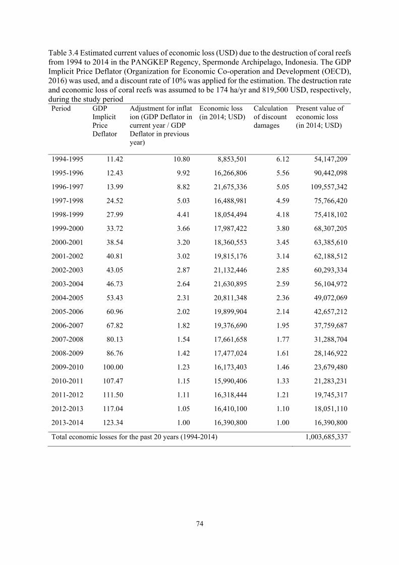
74
Table 3.4 Estimated current values of economic loss (USD) due to the destruction of coral reefs from 1994 to 2014 in the PANGKEP Regency, Spermonde Archipelago, Indonesia. The GDP Implicit Price Deflator (Organization for Economic Co-operation and Development (OECD), 2016) was used, and a discount rate of 10% was applied for the estimation. The destruction rate and economic loss of coral reefs was assumed to be 174 ha/yr and 819,500 USD, respectively, during the study period Period GDP
Implicit Price Deflator
Adjustment for inflation (GDP Deflator incurrent year / GDP Deflator in previous year)
Economic loss (in 2014; USD)
Calculation of discount damages
Present value of economic loss (in 2014; USD)
1994-1995 11.42 10.80 8,853,501 6.12 54,147,209
1995-1996 12.43 9.92 16,266,806 5.56 90,442,098
1996-1997 13.99 8.82 21,675,336 5.05 109,557,342
1997-1998 24.52 5.03 16,488,981 4.59 75,766,420
1998-1999 27.99 4.41 18,054,494 4.18 75,418,102
1999-2000 33.72 3.66 17,987,422 3.80 68,307,205
2000-2001 38.54 3.20 18,360,553 3.45 63,385,610
2001-2002 40.81 3.02 19,815,176 3.14 62,188,512
2002-2003 43.05 2.87 21,132,446 2.85 60,293,334
2003-2004 46.73 2.64 21,630,895 2.59 56,104,972
2004-2005 53.43 2.31 20,811,348 2.36 49,072,069
2005-2006 60.96 2.02 19,899,904 2.14 42,657,212
2006-2007 67.82 1.82 19,376,690 1.95 37,759,687
2007-2008 80.13 1.54 17,661,658 1.77 31,288,704
2008-2009 86.76 1.42 17,477,024 1.61 28,146,922
2009-2010 100.00 1.23 16,173,403 1.46 23,679,480
2010-2011 107.47 1.15 15,990,406 1.33 21,283,231
2011-2012 111.50 1.11 16,318,444 1.21 19,745,317
2012-2013 117.04 1.05 16,410,100 1.10 18,051,110
2013-2014 123.34 1.00 16,390,800 1.00 16,390,800
Total economic losses for the past 20 years (1994-2014) 1,003,685,337

75
Figure 3.1 Demand function of the coral reef benefits related to the fisheries using the
effect on production (EOP) method for: (a) the coral reef fish catch, (b) the crab catch,
(c) the squids and octopuses catch and (d) seaweed farming
76
Chapter IV General Discussion
4.1 Threats on coral reefs in the PANGKEP Regency Coral reefs in the Pangkajene and Kepulauan (PANGKEP) Regency are one of
the most important ecosystems in the area, as habitats for commercial fish species, tourists’
destination, research targets and coastal barriers and so on. Recently these reefs have been
under pressure of degradation due to human activities, including destructive fishing
practices (DFP), inflow of terrestrial total suspended matter (TSM), ineffective law
enforcement, no alternative income and lack of awareness of the fishermen, and rising
sea surface temperature (SST).
4.1.1 Destructive fishing issues
Damage of coral reef ecosystems damage due to DFP, was generally prominent
within the area far from mainland Sulawesi, from middle inner zone to outer zone.
Incidentally, coral reefs in these areas were commonly far from coastal lines, which is
difficult to monitor from the land. In contrast, damage of coral reefs close to the mainland
Sulawesi (inner zone) was considered to be normally caused by inflow of terrestrial TSM,
discharged from 6 estuaries along the coast of mainland Sulawesi between Makassar City
and the PANGKEP Regency.
Brant (1984) has classified all the world's fishing methods into 16 major groups,
which includes destructive fishing methods. In the Southeast Asia, devices used for
destructive fishing activities are generally chemicals (for cyanide fishing) and explosives
such as dynamites (for blast fishing). Technically, the cyanide fishing is to paralyze fish
through spraying cyanide into coral caves, while the blast fishing is to paralyze fish
mechanically by blasting, especially in coral reefs (Brant 1984).
The DFP, historically started in 1945’s, the first generation of DFP practitioners
were trained by Japanese Army during the World War II and were impressed by the
relatively easy operation and low costs to catch a large amount of fish by using dynamite
to blast the coral reefs. The type of explosive used has been evolved from dynamite to
homemade fertilizer-kerosene bombs. The blasting technique remains one of the main
options practiced by many fishermen in Indonesia, notably in the South Sulawesi (Pet-
Soede and Erdmann 1998), and these blasting activities were still found despite the status
of the area as a part of Coral reef rehabilitation and management program (COREMAP).
The existence of marine conservation area in the west part of the South Sulawesi Province
i.e. the Kapoposang Marine Protected Areas (MPAs), has yet to be effectively set as a
77
model of sustainable use of coral reefs, owing to low performance of management in the
MPA. The low performance, in turn, was caused by limited facility and lack of human
resource.
4.1.2 Law enforcement issues
Other factors including the lack of law enforcement need new resolution
especially enforcement related to the Police Institution of the PANGKEP Regency. Based
on observation and interview with key stakeholders in the research area, it was found that
several police officers were involved indirectly in the DFP as backup or by receiving
fisheries products or money as bribes. The corrupted law enforcement system in this area
encourages illegal activities. Therefore, leadership to improve the environmental issues
in the PANGKEP Police Institution is considered as a key factor for the success of marine
law enforcement.
Based on the results above, the following are suggested as possible options to
solve the law enforcement institution issues: 1) Improving the guidance of integrity,
ability, order and legal awareness to the law officers regarding their duties and
responsibilities; 2) Providing legal education, both formal and informal, to the public
about the importance of law enforcement in the sea so that people are aware of and follow
the prevailing regulations; 3) Improving the welfare of law officers to minimize law
enforcers’ involvement in corruption cases; and 4) Providing strict sanctions to the law
officers who do not perform their duties properly.
4.1.3 Land-based pollution issues
Pollution of the sea by land-based materials including total suspended matter
(TSM) has threatened the coral reef ecosystems, especially in the inner zone. Higher TSM
concentration than the permissible value (10 mg/L) is considered to disturb coral growth
in the 20 years from1994 to 2014. It was concluded that the highest concentration of TSM
in the inner zone had seasonality and was obviously higher around 190-223 mg/L in the
rainy season than in the dry season of 120-203 mg/L.
Several activities in the upland such as cement industry by limited liability
companies (LLC) (i.e. Semen Tonasa and Semen Bosowa), building residential
complexes, rice cropping and aquaculture in coastal areas, are all suspected as sources of
sediment materials discharged to the coastal waters. The sediment materials are
transported to the sea through river mouths and canals along the coast from Makassar
City to the PANGKEP Regency. In this case, rainfall plays an important role in
78
transporting sediments to the coastal region and subsequently affecting marine
ecosystems.
In order to solve the problem regarding to the environmental damage and
protection, the Indonesian Government issued several regulations including
Environmental Protection and Management Act No. 32 in 2009 and Coastal and Small
Island Management Act No. 1 in 2014. These regulations explicitly oblige the
corporations or individuals to preserve the environment and to avoid any
damages/pollutions, which might occur in all the phases of their business activities, i.e.
planning, production and post-production. However, the lack of awareness of
corporations or individuals regarding these regulations makes the environmental damages
and pollutions still prevalent. Besides, the lack of law enforcement by government bodies
also makes the regulations ineffective to prevent the environmental problems.
4.1.4 Socio-economic issues
Socio-economic factors related to fishermen living within coral reef area in the
PANGKEP Regency affect the coral reef ecosystems as natural resource. Low education
level and lack of awareness about the importance of coral reefs trigger the destructive
fishing practice. Other triggers include low income level and no alternative livelihoods.
In the study area, these were the boosting factors for individuals (fishermen) to conduct
destructive fishing to fulfil daily needs of their family without any significant
consideration of its long-term ecological impact. A social survey to key stakeholders
revealed that perpetrators of the DFP was primary resulting from low education level,
lack of awareness and no alternative livelihood and low income.
To solve this issue, planning of new comprehensive policies is considered to be
necessary. The policy must be responding several crucial points: 1) lack of educational
facilities and teaching staffs, 2) lack of access to business capitals, 3) high operational
costs of fishing, 4) further fishing locations from the settlements of traditional fishermen,
5) high prices of commodities which leads to capital loss of fisheries people.
4.2 Value of coral reefs in the PANGKEP Regency Coral reef destruction in this area is considered to be a result of low appreciation
of the value of the ecosystems by the local stakeholders. In other word, the local
stakeholders still undervalue the real worth of benefits produced by coral reef ecosystems,
which leads to the degradation. Economic valuation is an approach used to measure the
degree of local appreciation to the coral reefs by comparing the prices of service or good
given by the local stakeholders with the real whole values of the coral reefs.

79
In spite of the degradation, the coral reefs in the PANGKEP Regency still benefit
to the local community and the environment. Direct benefits could be calculated using
monetarily, while the indirect benefits could not be quantified monetarily. However, as
the whole, it is concluded that the coral reefs in this area possess high tangible and
intangible value. Tangible values generally consist of consumable or non-consumable use
values, e.g. fishery and tourism, while intangible values are non-use benefits or costs
needed for long-term ecosystem maintenance.
The "non-use" benefits related to the coral reef conservation for future generations
(i.e. bequest value) consisted of 98% of the total economic value of coral reefs in the
PANGKEP Regency. The high portion was estimated because of the relatively wide area
of coral reefs of 4,236 ha and high bequest value. According to a previous study (Boutwell
and Westra 2013), there were no references for the bequest value of coral reefs in the
PANGKEP Regency, and therefore, the bequest value in the Wakatobi MPAs with similar
characteristics and geography was referred to Hargreaves-Allen’s value in 2004
(Hargreaves-Allen 2004).
The high bequest value indicates that coral reefs in the PANGKEP Regency could
be the source of livelihood for future generations when the local community within the
area shows great awareness and activities of saving coral reef ecosystems.
4.3 Designing effective marine protected areas (MPAs) To anticipate the progressing coral cover degeneration and to ensure the
sustainability of ecosystem function in study area, establishment of MPAs is considered
to be necessary. The MPAs have been established in various coral reefs to manage
fisheries, biodiversity conservation, habitat restoration, tourism and the other human
activities in effective and sustainable ways (e.g. Ward and Hegerl 2003; Sumaila and
Charles 2002; Christie and White 2007).
Specifically, the benefit expected by the presence of MPAs is the restoration of
fish stock and ecosystem function. The sustainable benefit includes the spillover effect of
fish larvae from MPAs to the surrounding non-MPAs. The spillover effect enables to
provide additional fish stocks outside of the MPAs while maintaining the fish stocks
inside the MPAs (Figure 4.1). Even though the expectation had been review in several
references (Lauenroth and Burke 2008; Carpenter and Springer 2005; Roberts et al. 2002;
Spalding and Green 2001; Weeks et al. 2010; White et al. 2000), several empirical studies
had been conducted to elucidate the real function of MPAs. Therefore, integrated
approaches are needed to design future MPAs by involving local communities. Local
80
involvement in the planning, designing, establishing and managing MPAs is considered
to be crucial to make MPAs effective in long term period.
Coral reef exploitation inside the MPAs are not only related to fisheries but also
to tourism since the environment-friendly nature of this sector, and it is considered that
tourism could improve the economic condition of local people which may lead to coral
reef protection. In this study, economic value of coral reefs related to the tourism both
inside and outside MPAs was calculated for 2014. The result shows that the economic
value was estimated to be USD 108,462 inside the MPAs (i.e. in the Kapoposang Island),
while the value was around USD 7,700 outside the MPAs (i.e. in the Panambungan
Island). Therefore, coral reefs within MPAs could provide relatively high economic value
compared to those outside MPAs, showing the effectiveness of MPAs for saving coral
reefs.
4.4 Future perspective of the study Referring to the results and the limitations of this study, several important issues
related to stressors for the coral reef ecosystems are found to be solved. Sources of
stressors for coral reefs can be divided into two categories, namely natural and
anthropogenic factors. Natural factors include high sea surface temperature (SST),
rainfall, predators such as the crown-of-thorns starfish (COTs) and so on. Anthropogenic
factors include terrestrial industries that change the land-use pattern and causes excessive
discharge of the TSM into the sea and destructive fishing as elucidated in this study.
This study found that the dynamics of the TSM in coastal waters were strongly
related to land-use patterns and variability of the rainfall in the study sites. However,
further studies are necessary to elucidate the detailed changes in the land-use patterns and
the relationship with the seasonal change of the TSM concentration in the coastal waters.
The presence of the TSM in the coastal waters disrupts coral’s growth because the TSM
covers coral polyps and inhibit the photosynthesis by the symbiosis which is needed for
corals.
High SST is one of the threats that causes coral bleaching and potentially damages
the coral reefs in this area. Coral bleaching phenomena were found in the study area from
the end of 2009 to mid-2010 (Yusuf and Jompa 2012) and from mid-February to March
2016 (Syafyuddin Yusuf of Hasanuddin University, per. com.). So far, however, the total
area of coral bleaching cannot be evaluated in detail in the study site. Therefore, further
studies are necessary to clarify the distribution of SST and the relationship with coral reef
ecosystems in the study site.
81
Combination of both natural and anthropogenic stressors on coral reefs has given
a massive pressure which ultimately leads to increase in dead corals. Therefore, in the
future, combined threats to coral reefs are needed to be studied to develop more
comprehensive strategies to balance between saving coral reefs and enhancing local
economic growth in the study site.
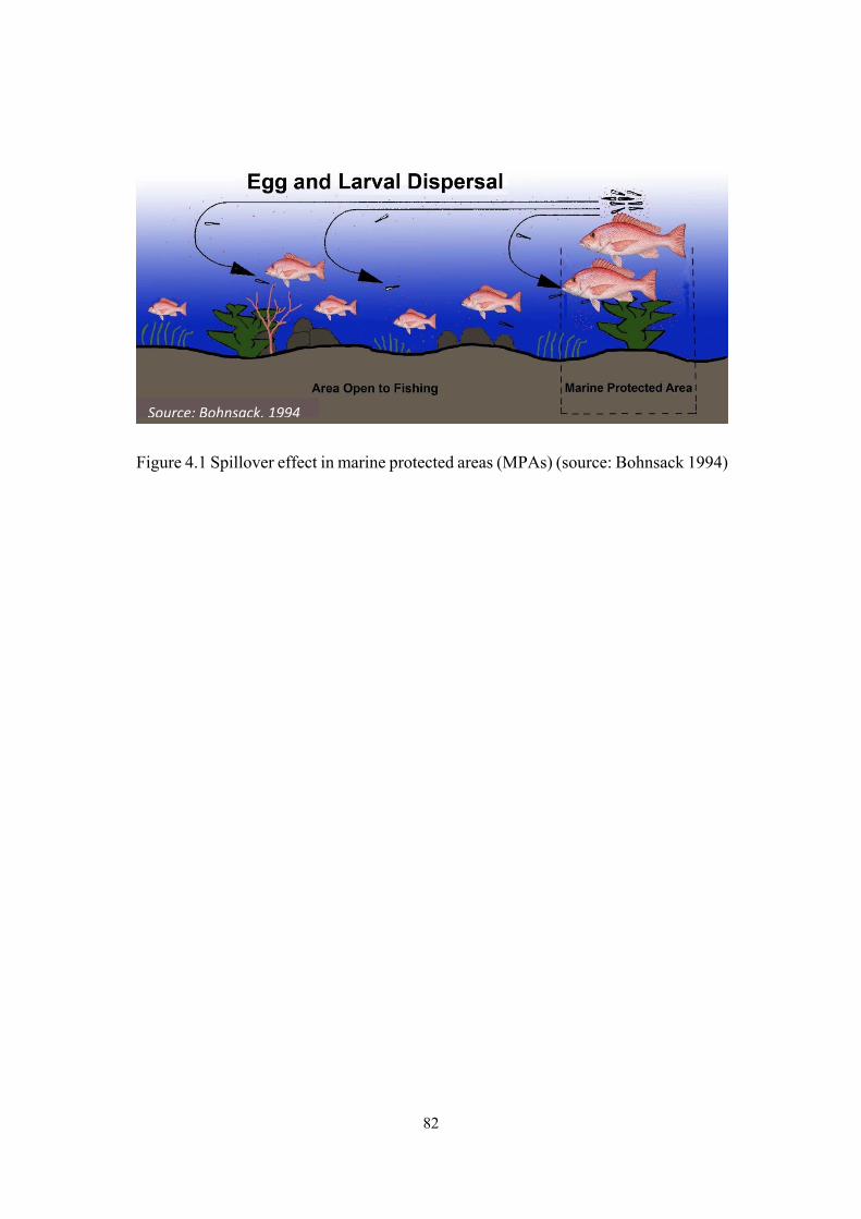
82
Source: Bohnsack, 1994
Figure 4.1 Spillover effect in marine protected areas (MPAs) (source: Bohnsack 1994)

83
Chapter V Conclusion
This study highlights a comprehensive analysis of the changes of coral reefs in the
last 20 years from 1994 to 2014 in the Pangkajene and Kepulauan (PANGKEP) Regency,
Spermonde Archipelago in Indonesia. That discusses the changes of coral reef habitats
and the causal factors of their changes, total economic benefit values and losses of total
direct economic benefit values. The first phase of the analysis conducted in this study was
calculation of the area of habitat of coral reefs and their physical changes in the last 20
years using remote sensing technology.
The results of analysis using multi-temporal land satellite (LANDSAT) imagery
data that include data derived from LANDSAT 5 thematic mapper (TM 1994),
LANDSAT 7 enhanced thematic mapper (ETM 2002) and Landsat 8 operational land
imager (OLI 2014) and in-situ measurement data indicate that the inter-annual change of
coral cover was substantial. The habitats of coral reefs experienced severer physical
damage from 2002-2014 than from 1994 to 2002, suggesting that coral degradation has
been accelerated recently. The decrease in coral reef habitats in the PANGKEP Regency,
Spermonde Archipelago is considered to be caused by two factors that include over-
sedimentation of harmful particles and destructive fishing practices. Spatially, destruction
of coral reefs at shoreline areas (inner zone) nearby the Sulawesi Island’s mainland was
dominated by sedimentation of harmful particles than destructive fishing activities. By
contrast, coral reef areas that were quite far away from the Sulawesi’s mainland (middle
inner zone, middle outer zone and outer zone) were dominated by destructive fishing
activities.
Referring to economic dimension, destruction of coral reefs in this area led to
significant loss of coral reef benefit value as a source for supplying goods and services.
It was estimated that the total economic loss due to coral reef destruction from 1994 to
2014 was USD 1 billion or 50.18 million USD/year. The loss of economic benefit value
designated as the total direct benefit value of coral reefs consisted of coral fish catch,
crabs catch, squid and octopuses catch, seaweed farming, tourism, scientific research and
shoreline protection. Nevertheless, the total economic value of coral reefs (use value and
non-use value) was approximately estimated to be USD 12.0 billion or 2.8 million
USD/ha. For example, most (99.8%) of the economic value was derived from non-use
value. The rest of the economic value was by coastal protection (USD 17 million)
followed by coral reef-related fisheries (USD 3 million), tourism and recreation (USD
116 thousand) and researches (USD 16 thousand). It was estimated that the economic
84
benefit values of coral reefs were declined along with the increase of adverse changes in
coral cover in the study area. In fact, it is important to consider particularly the threats to
the coral reefs. In order to reduce the threat on coral reefs, several potential practices
could be adopted: 1) selection of appropriate fishing gears, 2) development of an
alternative livelihood for small and traditional fishermen, 3) environmental education to
improve public awareness, 4) price standardization of fishery products to stabilize
fishermen’s income, and 5) strict law enforcement and severe penalties to prevent
destructive fishing practices.
Nowadays, many studies including this study give attention to the crises that
occurred in coral reef ecosystems. Regarding the research contribution, there were many
benefits than can be obtained from this dissertation not only for academic purposes but
the practical planning in response to the changing ecosystems of coral reefs and its socio-
economic values. Firstly, from the academic perspective, the method used in this
dissertation presented a viable framework for analyzing the changes on coral reefs in the
wide area with remote sensing approach and economic valuation approach. Secondly, the
results of this study can be used as a scientific basis for formulating policy strategies on
coral reef ecosystem management. From this perspective, local governments are
recommended to build new marine protected areas (MPAs) as one of the coral reef
governance strategies, so that coral reefs within MPAs could be managed effectively by
using zonation system (i.e., core zones, buffer zones and utilization zones).

85
Acknowledgments
The author would like to express his gratitude to:
1. Indonesia Endowment Fund for Education Scholarship (LPDP), Ministry of Finance,
Republic of Indonesia for immense support during the doctoral course.
2. Ministry of Research, Technology and Higher Education of Republic of Indonesia for
their support during the doctoral course.
3. Assoc. Prof. Masahiko Fujii for his guidance and patience as supervisor, and
facilitating books and travels needed for research activities.
4. Professors Masahiro Nakaoka, Shunitz Tanaka, Teiji Watanabe, and Masaaki
Kurasaki of Graduate School of Environmental Science, Hokkaido University and
Associate Prof. Junichi Kurihara of Graduate School of Science, Hokkaido University
for their review in order to improve this dissertation.
5. Prof. L.M. Aslan, Prof. Ma’ruf Kasim, Dr. Baru Sadarun of Faculty of Fisheries and
Marine Science of Halu Oleo University for their recommendations.
6. Prof. Jamaluddin Jompa, Prof. Sudirman, Dr. Rijal Idrus, Dr. Syafyuddin Yusuf, Dr.
Nurjannah Nurdin, Dr. Irwan Muliawan, Dr. Abd Gaffar, Haris Sunendar, M.Sc., Heri
Santoso, M.Sc., Ahmad Mauliddin, M.Sc., Hijaz Jalil, M.Si., Urban Elfatih, M.Sc.,
Amadhan Takwir, M.Si., for their invaluable insights for this research.
7. My parent La Ode Haya and Sitti Safia for the guidance, prayers and all their support
for higher education. Also my brothers and sister; La Ode Suryadin, La Ode Hamsar,
La Ode Hasrun, Soeherman, Rahmat Hidayat, Alimul Alam, and Neni Ramayanti for
all their motivation.
8. Dr. Wa Ode Salma – my wife and my children; Wa Ode Alifya Fatimah Azzahroh,
Ilham Wicaksana, Dolfy Saleh, and Cindy Priscilla for being my source of joy,
inspiration, and for always encouraging my thoughts with ways to be a better person.
9. Persatuan Pelajar Indonesia (PPI) in Hokkaido, Lembaga Pengelola Dana Pendidikan
(LPDP) group in Hokkaido, and Kajian Jumat Malam Fellows, especialy to Eko
Siswoyo, Erik Prasetyo Zen, Naufal Rospriandana, Rochim Bakti Cahyono,
Suherman, Achmad Syaifuddin, Harri, Ahmad, Lubis, Ade Purwanto, Haryo Edi
Wibowo, Lesnanto, Wahyu Kurnia, Freddy, Vecky Kuswandoro, Jamal Musa Hole,
Doddy Juli Irawan, Desi Utami, Zetryana, Isma Rosyida, Alfian Helmi, and Akhid
Sybli.
10. Team of Marine Science Diving Club (MSDC) of Hasanuddin University, especially
to Wawan Mangile, Syamsu Rijal, Tarsan, Neni Asriani, Andi Chaeryah, Nuryanti,
86
Asirwan, Nur Ismayanti, Nizar Hardiansyah, Januardi Septian. Also, Kapoposang of
Marine Protected Areas (MPAs) Crew, especially to Muh. Lukman, Bobby Adirianto,
Ilham, and Yaser Sakita.
This study was supported by the ”Precise Impact Assessments on Climate Change”
of the Program for Risk Information on Climate Change (SOUSEI Program) and the
“Integrated Research Program for Advancing Climate Models (TOUGOU Program)”
from the Ministry of Education, Culture, Sports, Science and Technology (MEXT),
Japan, the Environment Research and Technology Development Funds (S-15:
Predicting and Assessing Natural Capital and Ecosystem Services) of the Ministry of
the Environment, Japan, and the Belmont Forum “TSUNAGARI” fund by Japan
Science and Technology Agency.

87
References
Adrianto L (2006) Synopsis of the Introduction to Concepts and Methodology of
Economic Valuation of Coastal and Marine Resources. Center for Coastal and Marine
Resources Studies-Working papers, Bogor Agricultural University, Bogor
Aoun D (2015) Who pays more to preserve a natural reserve, visitors or locals? A
confidence analysis of a contingent valuation application. Environmental Economics and
Policy Studies 17(4): 471-486
Aronson RB, Precht WF (2001) Evolutionary paleoecology of Caribbean coral
reefs. Evolutionary paleoecology: the ecological context of macro evolutionary change.
Columbia University Press, New York, pp.171-233
Augustinus PGEF (2001) Sustainable management of the coastal area of SW Sulawesi,
Indonesia. In: Kaleidoscopic View on Social Scientific Global Change Research in the
Netherlands. Netherlands HDP Committee, Royal Academy of Arts and Sciences: 99-
107.
Baboo SS, Devi MR (2011) Geometric correction in recent high resolution satellite
imagery: a case study in Coimbatore, Tamil Nadu. International Journal of Computer
Applications 14: 32-37
Bohnsack JA (1994) How marine fishery reserves can improve fisheries. Proc. Gulf
Carib. Fish. Inst. 43: 217-241
Boschetti L, Flasse SP, Brivio PA (2004) Analysis of the conflict between omission and
commission in low spatial resolution dichotomic thematic products: The Pareto
Boundary. Remote Sensing of Environment 91: 280-292
Boutwell JL, Westra JV (2013) Benefit transfer: A review of methodologies and
challenges. Resources, 2(4): 517-527
Boyd J (2010) Lost ecosystem goods and services as a measure of marine oil pollution
damages. Resources for the Future Discussion Paper. 25 pp.
Brander LM, Beukering VP, Cesar HS (2007) The recreational value of coral reefs: a
meta-analysis. Ecological Economics 63 (1): 209-218
88
Brandt AV (1984) Fish Catching Methods of the World. Fishing News Books Ltd.
London. 534 pp.
Bridge TC, Hughes TP, Guinotte JM, Bongaerts P (2013) Call to protect all coral
reefs. Nature Climate Change 3(6): 528-530
Brown BE (1997) Disturbances to reefs in recent times. Life and death of coral reefs,
pp.354-379
Bruno JF, Selig ER (2007) Regional decline of coral cover in the Indo-Pacific: timing,
extent, and sub regional comparisons. PLoS one, 2(8): 1-8
Burke L, Reytar K, Spalding M, Perry A (2011) Reefs at risk revisited. World resources
Institute, Washington DC. 130 pp.
Burke L, Selig E, Spalding M (2002) Reefs at risk in Southeast Asia World Resources
Institute, Washington DC. 72 pp.
Call KA, Hardy JT, Wallin DO (2003) Coral reef habitat discrimination using
multivariate spectral analysis and satellite remote sensing. International Journal of
Remote Sensing, 24: 2627-2639
Campbell J (1987) Introduction to Remote Sensing. Guilford Press, New York. 551 pp.
Carpenter KE, Springer VG (2005) The center of the center of marine shore fish
biodiversity: the Philippine Islands. Environmental biology of fishes, 72(4): 467-480
Cesar H (1996) Economic analysis of Indonesian coral reefs. World Bank Environment
Department Paper. Environment Economics Series. Agriculture Operations Country
Department III. East Asia and Pacific Region and Environment Department, The World
Bank, Washington DC. 97 pp.
Cesar HS (2000) Coral reefs: their functions, threats and economic value. Collected
essays on the economics of coral reefs, pp.14-39
Cesar H, Burke L, Pet-Soede L (2003) The Economics of Worldwide Coral Reef
Degradation. Cesar Environmental Economics Consulting, the Netherlands. 24 pp.
Chapin III FS, Zavaleta ES, Eviner VT, Naylor RL, Vitousek PM, Reynolds HL, Mack
MC (2000) Consequences of changing biodiversity. Nature 405(6783): 234-242

89
Chavez PS (1996) Image-based atmospheric corrections-revisited and improved.
Photogrammetric engineering and remote sensing 62: 1025-1035
Che N, Price J (1992) Survey of radiometric calibration results and methods for visible
and near infrared channels of NOAA-7,-9, and-11 AVHRRs. Remote sensing of
environment 41: 19-27
Chee YE (2004) An ecological perspective on the valuation of ecosystem services. Biol.
Conserv. 120: 549-565
Chozin M (2008) Illegal but common: Life of blast fishermen in the Spermonde
Archipelago, South Sulawesi, Indonesia (Doctoral dissertation, Ohio University)
Christie P, White, AT (2007) Best practices for improved governance of coral reef marine
protected areas. Coral Reefs 26: 1047–1056
Congalton RG, Green K (2008) Assessing the accuracy of remotely sensed data:
principles and practices. CRC press, Taylor & Francis group, New York. 210 pp.
Congedo L, Macchi S (2013) Investigating the Relationship between Land Cover and
Vulnerability to Climate Change in Dar Es Salaam. Working Paper. 58 pp.
Connell JH (1997) Disturbance and recovery of coral assemblages. Coral reefs, 16(5):
101-113
Costanza R, d Arge R, de Groot R, Farber S, Grasso M, Hannon B, Limburg K, Naeem
S, O Neill R, Paruelo J, Raskin R, Sutton P, Belt VDM (1997) The value of the world's
ecosystem services and natural capital. Nature 387 (15): 253-260
D’Angelo C, Wiedenmann J (2014) Impacts of nutrient enrichment on coral reefs: new
perspectives and implications for coastal management and reef survival. Current Opinion
in Environmental Sustainability 7: 82-93
Davies-Colley R, Smith D (2001) Turbidity, suspended sediment and water quality: a
review. J. Am. Water Works Assoc 37: 1085–1101
De’ath G, Fabricius KE, Sweatman H, Puotinen M (2012) The 27–year decline of coral
cover on the Great Barrier Reef and its causes. Proceedings of the National Academy of
Sciences 109(44): 17995-17999
90
DFW-Indonesia (2003) Profile of Destructive Fishing in Spermonde Islands.
http://dfw.or.id/wp-content/uploads/2011/publikasi/DF_REPORT_SPERMONDE.pdf.
Accessed 2 May 2014 (in Bahasa)
Driml S (1999) Dollar values and trends of major direct uses of the Great Barrier Reef
Marine Park. Research Publication 56. Great Barrier Reef Marine Park Authority,
Townsville, Australia. 15 pp.
Eakin CM, Nim CJ, Brainard RE, Aubrecht C, Elvidge C, Gledhill DK, Muller-Karger F,
Mumby PJ, Skirving WJ, Strong AE, Wang M (2010) Monitoring coral reefs from space.
Oceanography 23(4): 118-133
Edinger EN, Jompa J, Limmon GV, Widjatmoko W, Risk MJ (1998) Reef degradation
and coral biodiversity in Indonesia: effects of land-based pollution, destructive fishing
practices and changes over time. Marine Pollution Bulletin 36: 617-630
El-Askary H, Abd El-Mawla S, Li J, El-Hattab M, El-Raey M (2014) Change detection
of coral reef habitat using Landsat-5 TM, Landsat 7 ETM+, and Landsat 8 OLI data in
the Red Sea (Hurghada, Egypt). International Journal of Remote Sensing 35: 2327-2346
ERDAS (2008) ER Mapper User's Guide. ERDAS Inc., United State of America. 278 pp.
Erftemeijer PL, Riegl B, Hoeksema BW, Todd PA (2012) Environmental impacts of
dredging and other sediment disturbances on corals: a review. Marine Pollution
Bulletin 64: 1737-1765
Fabricius KE (2005) Effects of terrestrial runoff on the ecology of corals and coral reefs:
review and synthesis. Marine Pollution Bulletin 50: 125–146
Falkowski PG, Jokiel PL, Kinzie RA (1990) Irradiance and corals. In: Dubinsky Z (eds)
Ecosystems of the World 25: Coral Reefs. Elsevier, Amsterdam, pp. 89-107
FAO (1999) Indicators for sustainable development of marine capture fisheries. FAO
Technical Guidelines for Responsible Fisheries No.8. FAO, Rome. 68 pp.
FAO (2000) Application of Contingent Valuation Method in Developing Countries. FAO
Economic and Social Development Papers No. 146/200. FAO, Rome. 14 pp.
Fauzi A (2006) Ekonomi Sumberdaya Alam dan Lingkungan, Teori dan Aplikasi.
Penerbit Gramedia Pustaka Utama. Jakarta. 256 pp. ISBN 9792210423
91
Fleiss JL, Cohen J, Everitt BS (1969) Large sample standard errors of kappa and weighted
kappa. Psychological Bulletin 72: 323–327
Freeman III, Myrick A, Herriges JA, Kling CL (2014) The measurement of
environmental and resource values, theory and methods. RFF Press, New York. 479 pp.
Gardner TA, Côté IM, Gill JA, Grant A, Watkinson AR (2003) Long-term region-wide
declines in Caribbean corals. Science 301: 958–960
Gomez ED, Alino PM, Yap HT, Licuanan WY (1994) A review of the status of Philippine
reefs. Marine Pollution Bulletin 29: 62-68
Gomez ED, Yap HT (1988) Monitoring reef condition. In: Kenchington RA, Hudson
BET (eds) Coral Reef Management Handbook. UNESCO Regional Office for Science
and Technology for Southeast Asia (ROSTSEA), Jakarta, pp. 171-178
Goodman JA, Purkis SJ, Phinn SR (2013) Coral reef remote sensing: A guide for
mapping, monitoring and management. Springer Science & Business Media, USA. 446
pp.
Green EP, Mumby PJ, Edwards AJ, Clark CD (2000) Remote sensing handbook for
tropical coastal management. UNESCO Publishing, Paris. 328 pp.
Grigalunas TA, Congar R (1995) Environmental economics for integrated coastal area
management: valuation methods and policy instruments. UNEP Regional Seas Reports
and Studies (UNEP). 175 pp.
Haapkylä J, Unsworth RKF, Flavell M, Bourne DG, Schaffelke B, Willis BL (2011)
Seasonal Correction:Seasonal Rainfall and Runoff Promote Coral Disease on an Inshore
Reef. PLoS ONE 6(3): 1-10
Hadjimitsis DG, Papadavid G, Agapiou A, Themistocleous K, Hadjimitsis MG, Retalis
A, Michaelides S, Chrysoulakis N, Toulios L, Clayton CR (2010) Atmospheric correction
for satellite remotely sensed data intended for agricultural applications: impact on
vegetation indices. Natural Hazards and Earth System Sciences 10: 89-95
Harbord RM, Higgins JP (2008) Meta-regression in Stata. Meta, 8(4): 493-519
92
Hargreaves-Allen V (2004) Estimating the Total Economic Value of Coral Reefs for
Residents of Sampela, a Bajau Community in Wakatobi Marine National Park,
Sulawesi. MSc dissertation, Imperial College London
Harley CD, Randall Hughes A, Hultgren KM, Miner BG, Sorte CJ, Thornber CS, and
Williams SL (2006). The Impacts of Climate Change in Coastal Marine Systems. Ecology
Letters 9(2): 228-241
Hedley JD, Roelfsema CM, Chollett I, Harborne AR, Heron SF, Weeks S, Skirving WJ,
Strong AE, Eakin CM, Christensen TR, Ticzon V (2016) Remote sensing of coral reefs
for monitoring and management: A review. Remote Sensing 8(118): 1-40
Hein MY, Lamb JB, Scott C, Willis BL (2015) Assessing baseline levels of coral health
in a newly established marine protected area in a global scuba diving hotspot. Marine
environmental research 103: 56-65
Hill J, Wilkinson C (2004) Methods for ecological monitoring of coral reefs. Australian
Institute of Marine Science, Townsville. 117 pp.
Hodgson G (1999) A global assessment of human effects on coral reefs. Marine Pollution
Bulletin 38: 345-355
Hoeksema BW (2012) Distribution patterns of mushroom corals (Scleractinia: Fungiidae)
across the Spermonde Shelf, South Sulawesi. Raffles Bull Zool 60: 183-212
Hopley D, Suharsono H (2000) The status of coral reefs in eastern Indonesia. Australian
Institute of Marine Science, Townsville. 144 pp.
Hourigan TF, Tricas TC, Reese ES (1988) Coral reef fishes as indicators of environmental
stress in coral reefs. Marine organisms as indicators 1988: 107-135
Howell DC (2016) Fundamental statistics for the behavioral sciences. Nelson Education.
676 pp.
https://cds-cv.nccs.nasa.gov/CREATE-V/ Accessed on June 2, 2017
http://kkji.kp3k.kkp.go.id/index.php/en/marine-protected-area-data/details/7/92.
Accessed on June 13, 2016
https://landsat.usgs.gov/. Accessed on April 1, 2017

93
http://www.miz.nao.ac.jp/staffs/nao99/index_En.html. Accessed on October 10, 2016
http://www.worldwildlife.org/publications/stewarding-biodiversity-and-food-security-
in-the-coral-triangle-achievements-challenges-and-lessons-learned. Accessed on
February 15, 2017
Hughes TP (1994) Catastrophes, phase shifts and lar ge-scale degradation of a Caribbean
coral reef. Science 265: 1547–1551
Hughes TP (1995) Catastrophes, phase shifts, and large-scale degradation of a Caribbean
coral reef. Biological Conservation 72(3), 411 pp.
Ishizaka J, Fukushima H, Kishino M, Saino T, Takahashi M (1992) Phytoplankton
pigment distribution in regional upwelling around the Izu Peninsula detected by coastal
zone color scanner on May 1982. Journal of Oceanography 48: 305-327
Jameson SC, Ammar M, Saadalla E, Mostafa HM, Riegl B (1999) A coral damage index
and its application to diving sites in the Egyptian Red Sea. Coral Reefs 18: 333-339
Jones GP, McCormick MI, Srinivasan M, Eagle JV (2004) Coral decline threatens fish
biodiversity in marine reserves. Proceedings of the National Academy of Sciences of the
United States of America 101: 8251-8253
Jones R, Bessell-Browne P, Fisher R, Klonowski W, Slivkoff M (2016) Assessing the
impacts of sediments from dredging on corals. Marine pollution bulletin 102: 9-29
Jones R, Ricardo GF, Negri AP (2015) Effects of sediments on the reproductive cycle of
corals. Marine pollution bulletin 100(1): 13-33
Jupiter S, Roelfsema CM, Phinn SR (2013) Science and Management. In: Goodman JA,
Purkis SJ, Phinn SR (eds.) Coral Reef Remote Sensing A Guide for Mapping, Monitoring
and Management. Springer, London, pp. 403-427
Komyakova V, Munday PL, Jones GP (2013) Relative importance of coral cover, habitat
complexity and diversity in determining the structure of reef fish communities. PloS one
8: 1-12
Kordi, O'Leary (2016) A spatial approach to improve coastal bioregion management of
the north Western Australia. Ocean & Coastal Management 127: 26-42

94
Krejcie RV, Morgan DW (1970) Table for determining sample size from a given
population. Educational and Psychological Measurement 30: 607-610
Lamy T, Galzin R, Kulbicki M, Lison de Loma T, Claudet J (2016) Three decades of
recurrent declines and recoveries in corals belie ongoing change in fish assemblages.
Coral reefs 35(1): 293–302
Lauenroth WK, Burke IC (2008) Ecology of the shortgrass steppe: a long-term
perspective. Oxford University Press. 537 pp.
Lillesand T, Kiefer RW, Chipman J (2004) Remote sensing and image interpretation.
John Willey &Sons Inc., New York. 812 pp.
Lillesand T, Kiefer RW, Chipman J (2014) Remote sensing and image interpretation.
John Wiley & Sons Inc. 146 pp.
Lubin D, Li W, Dustan P, Mazel CH, Stamnes K (2001) Spectral signatures of coral reefs:
Features from space. Remote sensing of environment 75: 127-137
Luczkovich JJ, Wagner TW, Michalek JL, Stoffle RW (1993) Discrimination of coral
reefs, seagrass meadows, and sand bottom types from space: A Dominician Republic
Case Study. Photogrametric Engineering & Remote Sensing 59: 385-389
Lyzenga DR (1978) Passive remote sensing techniques for mapping water depth and
bottom features. Applied optics 17: 379-383
Lyzenga DR (1981) Remote sensing of bottom reflectance and water attenuation
parameters in shallow water using aircraft and Landsat data. International Journal of
Remote Sensing 2: 71-82
Maple (2015) The Essential Tool for Mathematics.
https://www.maplesoft.com/products/maple/. Cited 10 November 2016
McManus JW (1997) Tropical marine fisheries and the future of coral reefs: a brief review
with emphasis on Southeast Asia. Coral Reefs 16: 121-127
Moberg F, Folke C (1999) Ecological goods and services of coral reef ecosystems.
Ecological Economics 29(2): 215-233. Doi: 10.1016/S0921-8009(99)00009-9
Moran PJ (1990) The Acanthaster planci (L); Biographical data. Coral Reefs 9: 95-96

95
Moran PJ (1988) Crown-of-thorns starfish: questions, answers. Australian
Institute of Marine Science. 35 pp.
Morton B (1994) Hong Kong's Coral Communities: Status, Threats and Management
Plans Marine Pollution Bulletin 29(1-3): 74-83
Mumby PJ (2001) Beta and habitat diversity in marine systems: a new approach to
measurement, scaling and interpretation. Oecologia 128: 274-280
Mumby P, Green E, Edwards A, Clark C (1999) The cost-effectiveness of remote sensing
for tropical coastal resources assessment and management. Journal of Environmental
Management 55: 157-166
Mumby PJ, Harborne AR (1999) Development of a systematic classification scheme of
marine habitats to facilitate regional management and mapping of Caribbean coral reefs.
Biological Conservation 88: 155-163
Mumby PJ, Hedley J, Chisholm JRM, Clark CD, Ripley H, Jaubert J (2004) The cover of
living and dead corals from airborne remote sensing. Coral Reefs 23: 171-183
Mumby PJ, Steneck RS (2008) Coral reef management and conservation in light of
rapidly evolving ecological paradigms. Trends in ecology & evolution 23: 555-563
NASA (2009) Millennium Reef Maps Metadata Updated 11 March 2009 For Landsat
images. http://oceancolor.gsfc.nasa.gov/LANDSAT/HTML/README.html. Accessed 1
September 2014
Nasr D (2015) Coral reefs of the Red Sea with special reference to the Sudanese Coastal
Area. In The Red Sea. Springer Berlin Heidelberg. pp. 453-469
Nurdin N, Grydehøj A (2014) Informal governance through patron–client relationships
and destructive fishing in Spermonde Archipelago, Indonesia. Journal of Marine and
Island Cultures 3(2): 54-59
Nurdin N, Komatsu T, AS MA, Djalil AR, Amri K (2015) Multisensor and multitemporal
data from Landsat images to detect damage to coral reefs, small islands in the Spermonde
archipelago, Indonesia. Ocean Science Journal 50: 317-325
96
Nurdin N, Prasyad H, Akbar ASM (2013) Dinamika Spasial Terumbu Karang pada
Perairan Dangkal Menggunakan Citra Landsat Di Pulau Langkai, Kepulauan
Spermonde. Jurnal Ilmiah Geomatika 19: 83-89 (in Bahasa with English abstract)
Organization for Economic Co-operation and Development – OECD (2016) GDP
Implicit Price Deflator in Indonesia.
https://fred.stlouisfed.org/series/IDNGDPDEFAISMEI. Cited 12 August 2016
Pagiola S, Bishop J, Ritter VK (2004) Assessing the economic value of ecosystem
conservation. Environment Department Paper No.101. The World Bank, Washington DC.
66 pp.
Palandro DA, Andréfouët S, Hu C, Hallock P, Müller-Karger FE, Dustan P, Callahan
MK, Kranenburg C, Beaver CR (2008) Quantification of two decades of shallow-water
coral reef habitat decline in the Florida Keys National Marine Sanctuary using Landsat
data (1984–2002). Remote sensing of environment 112: 3388-3399
Parwati E, Kartasasmita M, Soewardi K, Kusumastanto T, Nurjaya IW (2013) The
relationship between total suspended solid (TSS) and coral reef growth (case study of
Derawan Island, Delta Berau Waters). International Journal of Remote Sensing and Earth
Sciences (IJReSES) 10: 104-113
Pearce D, Moran D (2009) The Economic Value of Biodiversity. IUCN-The World
Conservation Union, London. 180 pp. ISBN: 978-1-85383-195-9
Pendleton LH, Hoegh-Guldberg O, Langdon C, Comte A (2016) Multiple Stressors and
Ecological Complexity Require a New Approach to Coral Reef Research. Frontiers in
Marine Science (3):36 pp.
Pet-Soede C (2000) Options for co-management of an Indonesian coastal fishery.
Dissertation, Wegenigen University, see
http://library.wur.nl/WebQuery/wurpubs/fulltext/121232
Pet-Soede L, Erdmann M (1998) An overview and comparison of destructive fishing
practices in Indonesia. SPC Live Reef Fish Information Bulletin 4: 28-36
Pet-Soede C, Cesar H, Pet J (1999) An economic analysis of blast fishing on Indonesian
coral reefs. Environmental Conservation 26(2): 83-93
97
Polónia AR, Cleary DF, de Voogd NJ, Renema W, Hoeksema BW, Martins A, Gomes
NC (2015) Habitat and water quality variables as predictors of community composition
in an Indonesian coral reef: a multi-taxon study in the Spermonde Archipelago. Science
of the total environment 537: 139-151
Porter JW, Meier OW (1992) Quantification of loss and change in Floridian reef coral
populations. American Zoologist 32(6): 625-640
Purkis SJ, Pasterkamp R (2004) Integrating in situ reef-top reflectance spectra with
Landsat TM imagery to aid shallow-tropical benthic habitat mapping. Coral Reefs 23: 5-
20
Radjawali I (2012) Examining local conservation and development: Live reef food
fishing in Spermonde Archipelago, Indonesia. Revista da Gestão Costeira
Integrada 12(4): 545-557
Research Center for Oceanography, Indonesian Institute of Sciences (2014) Handbook
of shallow water habitats mapping.
http://www.coremap.or.id/downloads/gis_1435730309.pdf. Accessed 30 September
2016 (in Bahasa)
Roberts CM (1997) Connectivity and management of Caribbean coral reefs. Science 278:
1454–1457
Roberts CM, McClean JC, Veron JEN, Hawkins JP, Allen GR, McAllister DE,
Mittermeier CG (2002) Marine biodiversity hotspots and conservation priorities for
tropical reefs. Science 295 (5558): 1280-1284
Roelfsema C, Phinn S, Dennison W (2002) Spatial distribution of benthic microalgae on
coral reefs determined by remote sensing. Coral Reefs 21: 264-274
Rogers A, Harborne AR, Brown CJ, Bozec YM, Castro C, Chollett I, Hock K, Knowland
CA, Marshell A, Ortiz JC, Razak T (2015) Anticipative management for coral reef
ecosystem services in the 21st century. Global change biology 21(2): 504-514
Salvat B (1987) Human Impacts on Coral Reefs: Facts and Recommendations. Antenne
Mussee, Ecole Pratique des Hautes Etudes, French Polynesia. 253 pp.
98
Samonte GP, Eisma-Osorio RL, Amolo R, White A (2016) Economic value of a large
marine ecosystem: Danajon double barrier reef, Philippines. Ocean & Coastal
Management 122: 9-19
Saunders M, Lewis P, Thornhill A (2007) Research Methods for Business Students. Essex,
UK: Pearson, Education Limited. 649 pp. ISBN 978-0-273- 70148-4
Sawyer DA (1992) Taka Bone Rate: management, development and resource valuation
of an Indonesian Atoll, MA thesis, Dept Economics, Dalhousie University, Halifax, Nova
Scotia
Scopélitis J, Andréfouët S, Phinn S, Chabanet P, Naim O, Tourrand C, Done T (2009)
Changes of coral communities over 35 years: Integrating in situ and remote-sensing data
on Saint-Leu Reef (la Réunion, Indian Ocean). Estuarine, Coastal and Shelf Science 84:
342-352
Sekaran U (2003) Research methods for Business, a skill-building approach, Fourth
Edition. John Wiley & Sons, Inc. ISBN 0-471-20366-1
Sinden JA (1994) A review of environmental valuation in Australia. Review of Marketing
and Agricultural Economics 62: 337–368
Souter DW, Linden O (2000) The health and future of coral reef systems. Ocean &
Coastal Management 43(8): 657-688
Spalding M, Ravilious C, Green EP (2001) World atlas of coral reefs. University of
California Press, Berkeley. 424 pp.
Statistics Indonesia of Pangkajene and Kepulauan Regency (2014)
https://PANGKEPkab.bps.go.id/index.php. Cited 10 October 2014
Statistics Indonesia of Pangkajene and Kepulauan Regency (2015)
https://pangkepkab.bps.go.id. Accessed 20 December 2016
Suharsono, Purnomohadi N (2001) International Coral Reef Initiative Country Report:
Indonesia, paper presented at the Regional ICRI Workshop for East Asia, Cebu,
Philippines. 13 pp.
Sumaila UR, Charles AT (2002) Economic models of marine protected areas: an
introduction. Natural Resource Modeling 15(3): 261-272

99
Suwargana N (2014) Analysis of Alos AVNIR-2 imagery for coral reefs mapping (A Case
Study: Banyuputih, Situbondo). Proceedings of the National Seminar on remote sensing,
Indonesian National Institute of Aeronautics and Space (LAPAN). pp. 588-596.
http://sinasinderaja.lapan.go.id/wp-content/uploads/2014/06/bukuprosiding_588-
596.pdf. Accessed 10 October 2014 (in Bahasa with English abstract)
Tseng WWC, Hsu SH, and Chen CC (2015) Estimating the willingness to pay to protect
coral reefs from potential damage caused by climate change-The evidence from
Taiwan. Marine pollution bulletin 101(2): 556-565
UNEP (2006) Marine and Coastal Ecosystems and Human Well-Being: A Synthesis
Report Based on the Findings of the Millennium Ecosystem Assessment. UN
Environment Programme, Nairobi. 76 pp.
Unsworth RE and Petersen TB (1995) A manual for conducting natural resource damage
assessment: the role of economics. Industrial Economics Incorporated.
https://www.fws.gov/policy/NRDAManualFull.pdf. Cited 13 June 2016
United States Geological Survey (2014) Data sets. https://earthexplorer.usgs.gov/.
Accessed on 20 December 2014
Wahiddin N, Siregar VP, Nababan B, Jaya I, Wouthuyzen S (2015) Change detection of
coral reef habitat using Landsat imagery in Morotai Island North Maluku Province. Jurnal
Ilmu dan Teknologi Kelautan Tropis 6: 507-524 (in Bahasa with English abstract)
Wahyudin Y (2007) An Economic Value of the Natural Seaweed Resources. Available
at SSRN 1678973. http://dx.doi.org/10.2139/ssrn.1678973
Ward TJ, Hegerl EJ (2003) The benefits of marine protected areas. Department of the
Environment and Heritage, Commonwealth of Australia. 77 pp.
Wawo M, Adrianto L, Bengen DG, Wardiatno Y (2014) Valuation of Seagrass
Ecosystem Services in Kotania Bay Marine Nature Tourism Park, Western Seram,
Indonesia. Asian Journal of Scientific Research 7(4): 591-600
Weeks R, Russ GR, Alcala AC, White AT (2010) Effectiveness of marine protected areas
in the Philippines for biodiversity conservation. Conservation Biology 24(2): 531-540
Weil E, Smith G, Gil-Agudelo DL (2006) Status and progress in coral reef disease
research. Diseases of aquatic organisms 69(1): 1-7

100
Weinberg S (1976) Submarine daylight and ecology. Marine Biology 37: 291-304
Wells S (2009) Dynamite fishing in northern Tanzania–pervasive, problematic and yet
preventable. Marine Pollution Bulletin 58(1): 20-23
Wilkinson CR (1992) Coral reefs of the w orld are facing widespread devastation: can we
prevent this through sustainable management practices? Proc. 7th International Coral
Reef Symposium 1: 11–21
Wilkinson CR (1996) Global change and coral reefs: impacts on reefs, economies and
human cultures. Global Change Biology 2(6): 547-558
Wilkinson CR (2008) Status of Coral Reefs of the World: 2008 Global Coral Reef
Monitoring Network and Reef and Rainforest Research Center. Townsville, Australia.
296 pp.
White AT, Vogt HP, Arin T (2000) Philippine coral reefs under threat: the economic
losses caused by reef destruction. Marine Pollution Bulletin 40(7): 598-605
Wooldridge SA, Brodie JE (2015) Environmental triggers for primary outbreaks of
crown-of-thorns starfish on the Great Barrier Reef, Australia. Marine pollution bulletin
101(2): 805-815
World Bank (2015) World Bank Supports Indonesia’s Coral Reefs and Coastal
Communities. http://www.worldbank.org/en/news/press-release/2014/02/21/world-
bank-indonesia-coral-reefs-coastal-communities. Accessed 15 July 2015
World Wild Fund (2016) Coral Triangle. http://www.worldwildlife.org/places/coral-
triangle. Accessed 20 December 2016
Yasir Haya LM, Fujii M (2017) Mapping the Change of Coral Reefs Using Remote
Sensing and in situ Measurements; A Case Study in PANGKEP Regency, Spermonde
Archipelago, Indonesia. Journal of Oceanography. DOI: 10.1007/S10872-017-0422-4
Yusuf S (2008) Outbreak Phenomenon of Acanthaster planci and its predatory due to
Scleratinian living preferences in Kapoposang Island, South Sulawesi. Proceeding of
Indonesian Coral Reef Symposium, 235-243
Yusuf S, Jompa J (2012) Indonesia First Quantitative Assessment of Coral Bleaching on
Indonesian Reefs. In: Proceedings of the 12th International Coral Reef Symposium.

101
Cairns, Australia.
http://www.icrs2012.com/proceedings/manuscripts/ICRS2012_17D_6.pdf
Zheng Z, Li Y, Guo Y, Xu Y, Liu G, Du C (2015) Landsat-Based Long-Term Monitoring
of Total Suspended Matter Concentration Pattern Change in the Wet Season for Dongting
Lake, China. Remote Sensing 7: 13975-13999
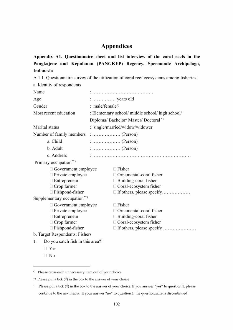
102
Appendices
Appendix A1. Questionnaire sheet and list interview of the coral reefs in the
Pangkajene and Kepulauan (PANGKEP) Regency, Spermonde Archipelago,
Indonesia
A.1.1. Questionnaire survey of the utilization of coral reef ecosystems among fisheries
a. Identity of respondents
Name : …………………………………
Age : …………… years old
Gender : male/female
Most recent education : Elementary school/ middle school/ high school/
Diploma/ Bachelor/ Master/ Doctoral *)
Marital status : single/married/widow/widower
Number of family members : ……………… (Person)
a. Child : ……………… (Person)
b. Adult : ……………… (Person)
c. Address : ………………………………………………………
Primary occupation**)
Government employee Fisher Private employee Ornamental-coral fisher Entrepreneur Building-coral fisher Crop farmer Coral-ecosystem fisher Fishpond-fisher If others, please specify………………
Supplementary occupation**)
Government employee Fisher Private employee Ornamental-coral fisher Entrepreneur Building-coral fisher Crop farmer Coral-ecosystem fisher Fishpond-fisher If others, please specify …………………
b. Target Respondents: Fishers
1. Do you catch fish in this area?1
Yes
No
Please cross each unnecessary item out of your choice
**) Please put a tick () in the box to the answer of your choice
1 Please put a tick () in the box to the answer of your choice. If you answer “yes” to question 1, please
continue to the next items. If your answer “no” to question 1, the questionnaire is discontinued.
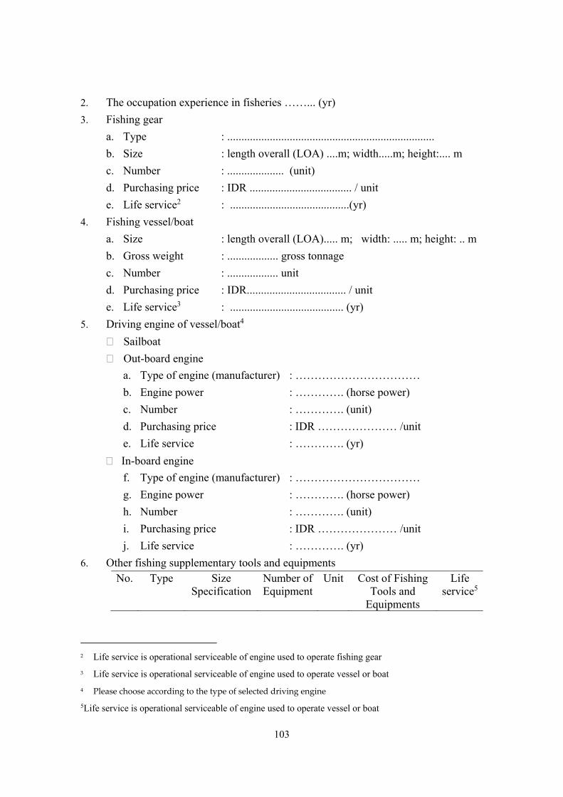
103
2. The occupation experience in fisheries ……... (yr)
3. Fishing gear
a. Type : .........................................................................
b. Size : length overall (LOA) ....m; width.....m; height:.... m
c. Number : .................... (unit)
d. Purchasing price : IDR .................................... / unit
e. Life service2 : ..........................................(yr)
4. Fishing vessel/boat
a. Size : length overall (LOA)..... m; width: ..... m; height: .. m
b. Gross weight : .................. gross tonnage
c. Number : .................. unit
d. Purchasing price : IDR................................... / unit
e. Life service3 : ........................................ (yr)
5. Driving engine of vessel/boat4
Sailboat
Out-board engine
a. Type of engine (manufacturer) : ……………………………
b. Engine power : …………. (horse power)
c. Number : …………. (unit)
d. Purchasing price : IDR ………………… /unit
e. Life service : …………. (yr)
In-board engine
f. Type of engine (manufacturer) : ……………………………
g. Engine power : …………. (horse power)
h. Number : …………. (unit)
i. Purchasing price : IDR ………………… /unit
j. Life service : …………. (yr)
6. Other fishing supplementary tools and equipments No. Type Size
SpecificationNumber of Equipment
Unit Cost of Fishing Tools and
Equipments
Life service5
2 Life service is operational serviceable of engine used to operate fishing gear
3 Life service is operational serviceable of engine used to operate vessel or boat
4 Please choose according to the type of selected driving engine
5Life service is operational serviceable of engine used to operate vessel or boat
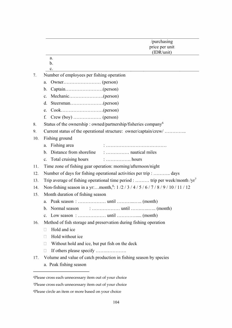
104
/purchasing price per unit
(IDR/unit) a. b. c.
7. Number of employees per fishing operation
a. Owner…………………… (person)
b. Captain……………………(person)
c. Mechanic………………….(person)
d. Steersman…………………(person)
e. Cook………………………(person)
f. Crew (boy) ……………… (person)
8. Status of the ownership : owned/partnership/fisheries company6
9. Current status of the operational structure: owner/captain/crew/ …………..
10. Fishing ground
a. Fishing area : …………………………………
b. Distance from shoreline : …………… nautical miles
c. Total cruising hours : ……………. hours
11. Time zone of fishing gear operation: morning/afternoon/night
12. Number of days for fishing operational activities per trip : ……….. days
13. Trip average of fishing operational time period : ……… trip per week/month /yr7
14. Non-fishing season in a yr:…month,8: 1 /2 / 3 / 4 / 5 / 6 / 7 / 8 / 9 / 10 / 11 / 12
15. Month duration of fishing season
a. Peak season : ……………… until ………...….. (month)
b. Normal season : ……………… until …….…..….. (month)
c. Low season : ……………… until …………..... (month)
16. Method of fish storage and preservation during fishing operation
Hold and ice
Hold without ice
Without hold and ice, but put fish on the deck
If others please specify …….………….
17. Volume and value of catch production in fishing season by species
a. Peak fishing season
6Please cross each unnecessary item out of your choice
7Please cross each unnecessary item out of your choice
8Please circle an item or more based on your choice
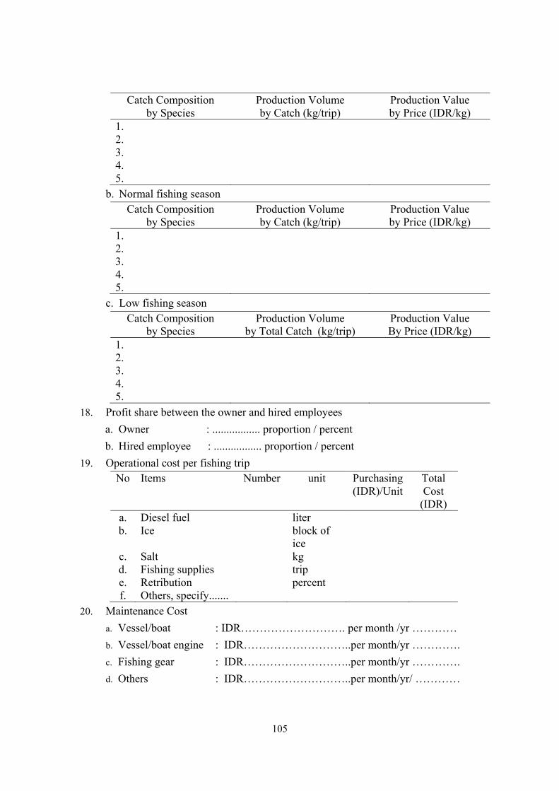
105
Catch Composition by Species
Production Volume by Catch (kg/trip)
Production Value by Price (IDR/kg)
1. 2. 3. 4. 5.
b. Normal fishing season Catch Composition
by Species Production Volume by Catch (kg/trip)
Production Value by Price (IDR/kg)
1. 2. 3. 4. 5.
c. Low fishing season Catch Composition
by Species Production Volume
by Total Catch (kg/trip) Production Value By Price (IDR/kg)
1. 2. 3. 4. 5.
18. Profit share between the owner and hired employees
a. Owner : ................. proportion / percent
b. Hired employee : ................. proportion / percent
19. Operational cost per fishing trip No Items Number unit Purchasing
(IDR)/Unit Total Cost
(IDR) a. Diesel fuel liter b. Ice block of
ice
c. Salt kg d. Fishing supplies trip e. Retribution percent f. Others, specify.......
20. Maintenance Cost
a. Vessel/boat : IDR………………………. per month /yr …………
b. Vessel/boat engine : IDR………………………..per month/yr ………….
c. Fishing gear : IDR………………………..per month/yr ………….
d. Others : IDR………………………..per month/yr/ …………
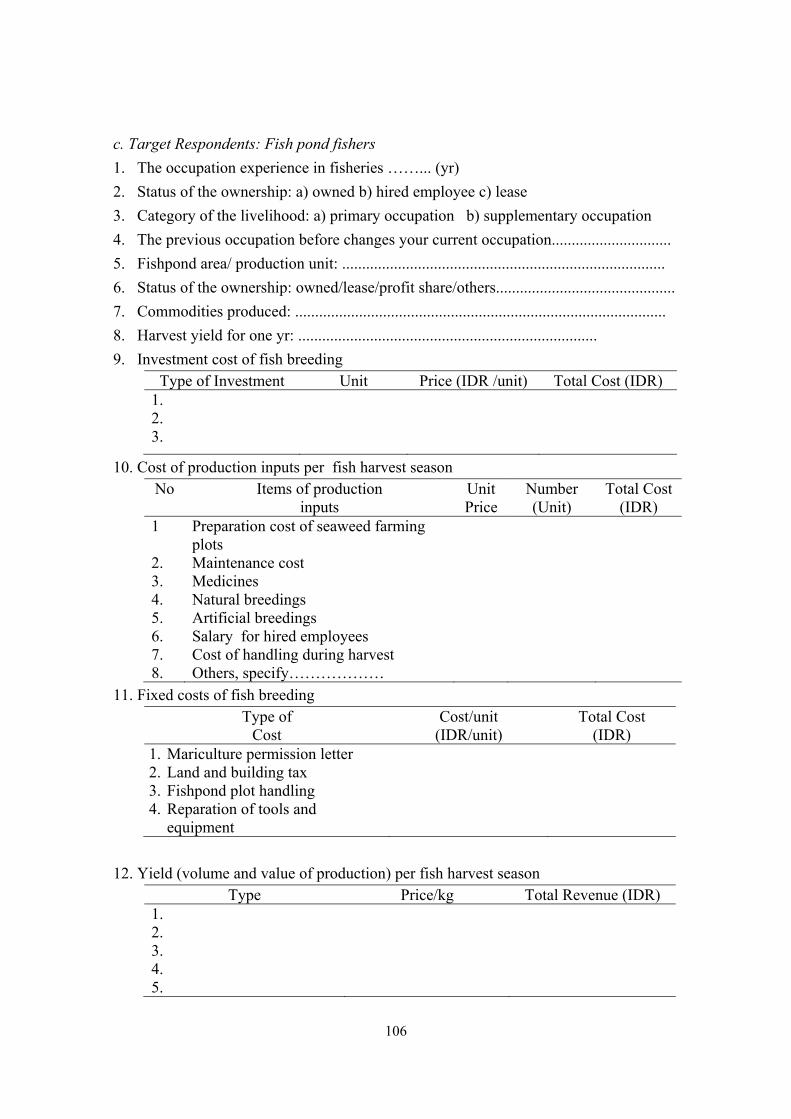
106
c. Target Respondents: Fish pond fishers
1. The occupation experience in fisheries ……... (yr)
2. Status of the ownership: a) owned b) hired employee c) lease
3. Category of the livelihood: a) primary occupation b) supplementary occupation
4. The previous occupation before changes your current occupation..............................
5. Fishpond area/ production unit: .................................................................................
6. Status of the ownership: owned/lease/profit share/others.............................................
7. Commodities produced: .............................................................................................
8. Harvest yield for one yr: ...........................................................................
9. Investment cost of fish breeding Type of Investment Unit Price (IDR /unit) Total Cost (IDR)
1. 2. 3.
10. Cost of production inputs per fish harvest season No Items of production
inputs Unit Price
Number (Unit)
Total Cost (IDR)
1 Preparation cost of seaweed farming plots
2. Maintenance cost 3. Medicines 4. Natural breedings 5. Artificial breedings 6. Salary for hired employees 7. Cost of handling during harvest 8. Others, specify………………
11. Fixed costs of fish breeding Type of
Cost Cost/unit
(IDR/unit) Total Cost
(IDR) 1. Mariculture permission letter 2. Land and building tax 3. Fishpond plot handling 4. Reparation of tools and
equipment
12. Yield (volume and value of production) per fish harvest season Type Price/kg Total Revenue (IDR)
1. 2. 3. 4. 5.
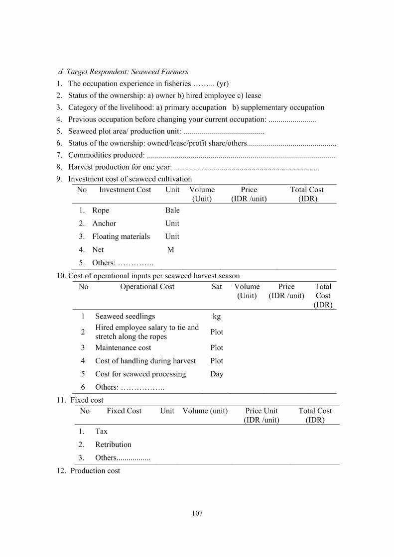
107
d. Target Respondent: Seaweed Farmers
1. The occupation experience in fisheries ……... (yr)
2. Status of the ownership: a) owner b) hired employee c) lease
3. Category of the livelihood: a) primary occupation b) supplementary occupation
4. Previous occupation before changing your current occupation: ........................
5. Seaweed plot area/ production unit: .........................................
6. Status of the ownership: owned/lease/profit share/others.............................................
7. Commodities produced: ...............................................................................................
8. Harvest production for one year: .........................................................................
9. Investment cost of seaweed cultivation No Investment Cost Unit Volume
(Unit) Price
(IDR /unit) Total Cost
(IDR)
1. Rope Bale
2. Anchor Unit
3. Floating materials Unit
4. Net M
5. Others: …………..
10. Cost of operational inputs per seaweed harvest season No Operational Cost Sat Volume
(Unit) Price
(IDR /unit) Total Cost
(IDR)
1 Seaweed seedlings kg
2 Hired employee salary to tie and stretch along the ropes
Plot
3 Maintenance cost Plot
4 Cost of handling during harvest Plot
5 Cost for seaweed processing Day
6 Others: ……………..
11. Fixed cost No Fixed Cost Unit Volume (unit) Price Unit
(IDR /unit) Total Cost
(IDR)
1. Tax
2. Retribution
3. Others.................
12. Production cost

108
No Cost Unit Volume (kg)
Price Unit (IDR)
1 Wet seaweed Kg
2 Dried seaweed Kg
3 Others: ……………..

109
A.1.2. Questionnaire survey of the utilization of coral reef ecosystem among tourists and
researchers
a. Identity of Respondents
1. Name: .....................................................................................................
2. Age : .....................................................................................................
3. Origin of place: ..........................................................................................
4. Most recent education : Elementary school/ middle school/ high school/
Diploma/ Bachelor/ Master/ Doctoral
5. Household income:
a. IDR 500.000 – 1.000.000
b. IDR 1.000.000 – 2.000.000
c. IDR 3.000.000 – 4.000.000
d. IDR 4.000.000 – 5.000.000
e. More than IDR 5.000.000
b. Tourist/researcher Activities
1. How many visitors who recreate with you in this area (tourism group) ..........persons
2. Tourism cost in this area
a. Transportation : IDR ............................/person
b. Lodging : IDR …………………/person
c. Food/Beverage : IDR ………………./person
d. Entrance ticket : IDR............................/person
e. Rent for entertainment facilities : IDR............................ /person
f. Charge for the use of public utilities (WC and others): IDR……………/person
g. Others, …………… : IDR…………/person
3. What your perception based on your tourism experience in this area?
Positive
Neutral
Negative
4. Number of your visits in this area ........................ visit/yr
5. How long do you spend your tourism experience per trip? .......................(day)
6. Probably you lose your productive time for spending your time in this area. How
many your productive loses converted into money?
IDR................................................

110
7. Is there any tourism destination as an alternative besides this tourism area?9
No
Yes
7a) If your answer to question 7 is “yes”, how much cost you spend at that tourism
destination
a. Transportation : IDR ............................../person
b. Lodging : IDR …………………/person
c. Food/Beverage : IDR ………………/person
d. Entrance ticket : IDR.............................../person
e. Rent for entertainment facilities : IDR.............................../person
f. Charge for the use of public utilities (WC and others): IDR………/person
g. Others, …………… : IDR…………/person
7b) How many times do you go to that tourism destination? .........
A.1.3. Questionnaire survey of local people living at the surrounding areas of coral reef
ecosystems
a. Characteristics of Respondents
Name : ………………………
Age : .................................. (yr)
Most recent education : Elementary school/ middle school/ high school/ Diploma/
Bachelor/ Master/ Doctoral
Number of family members : ……………. (person)
Current occupation :
Household income: IDR. ..................../yr
b. Knowledge/Perception of Respondents on Coral Reefs
1. Do you aware that the existence of coral reefs gives benefits to local peoples in this
area?
a. Strongly aware
b. Aware
c. Neither aware nor unaware
d. Unaware
e. Strongly unaware
If your answer to question 7 is “no“, this questionnare is discontinued, whereas, if your answer to
question 7 is “no“, the next questions is continued to no.7a) and 7b)
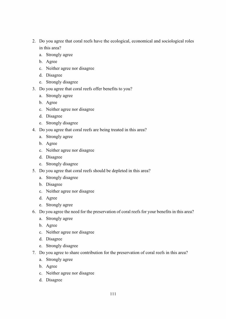
111
2. Do you agree that coral reefs have the ecological, economical and sociological roles
in this area?
a. Strongly agree
b. Agree
c. Neither agree nor disagree
d. Disagree
e. Strongly disagree
3. Do you agree that coral reefs offer benefits to you?
a. Strongly agree
b. Agree
c. Neither agree nor disagree
d. Disagree
e. Strongly disagree
4. Do you agree that coral reefs are being treated in this area?
a. Strongly agree
b. Agree
c. Neither agree nor disagree
d. Disagree
e. Strongly disagree
5. Do you agree that coral reefs should be depleted in this area?
a. Strongly disagree
b. Disagree
c. Neither agree nor disagree
d. Agree
e. Strongly agree
6. Do you agree the need for the preservation of coral reefs for your benefits in this area?
a. Strongly agree
b. Agree
c. Neither agree nor disagree
d. Disagree
e. Strongly disagree
7. Do you agree to share contribution for the preservation of coral reefs in this area?
a. Strongly agree
b. Agree
c. Neither agree nor disagree
d. Disagree

112
e. Strongly disagree
8. How much money (IDR) you spend for retribution in favor of the preservation of coral
reefs in this area in a yr? Please specify …………………………………...
9. What percent of your income spent for retribution in a year in favor of the preservation
of coral reefs in this area?
a. 1%
b. 2%
c. 3%
d. 4%
e. 5%
f. 6%
g. 7%
h. 8%
i. 9%
j. 10%
k. More than 10% (............%)
c. Complemental Data
Total populations living at surrounding areas of coral reef ecosystem
Area of coral coverage at surrounding areas
A.1.4. List question for interview
1. Do you have specific ties with your commercial-fisher?
a. Yes b. No
2. If your answer to question 1 is “yes“, what factors that motivate you to relate with
your commercial-fisher?
a. Credits for fishing investment (vessel/boat, fishing gear, etc), please
specify…………………………(IDR)
b. Credits for equipment supplies, please specify ..................................(IDR /trip)
c. If others please specify ...............................................................................
3. What benefits you have by to do social relation with your commercial-fisher? (yes/no).
If your answer is “yes“, please chose one or more the following items
a. Credit (money) used for lack of something important
b. Health benefit
c. Bonus receive near Holidays
d. If others please specify, ……………………………….............…………….
What detriments have you by to do social relation with your commercial-fisher?
(yes/no). If your answer is “yes“, please specify .................................................
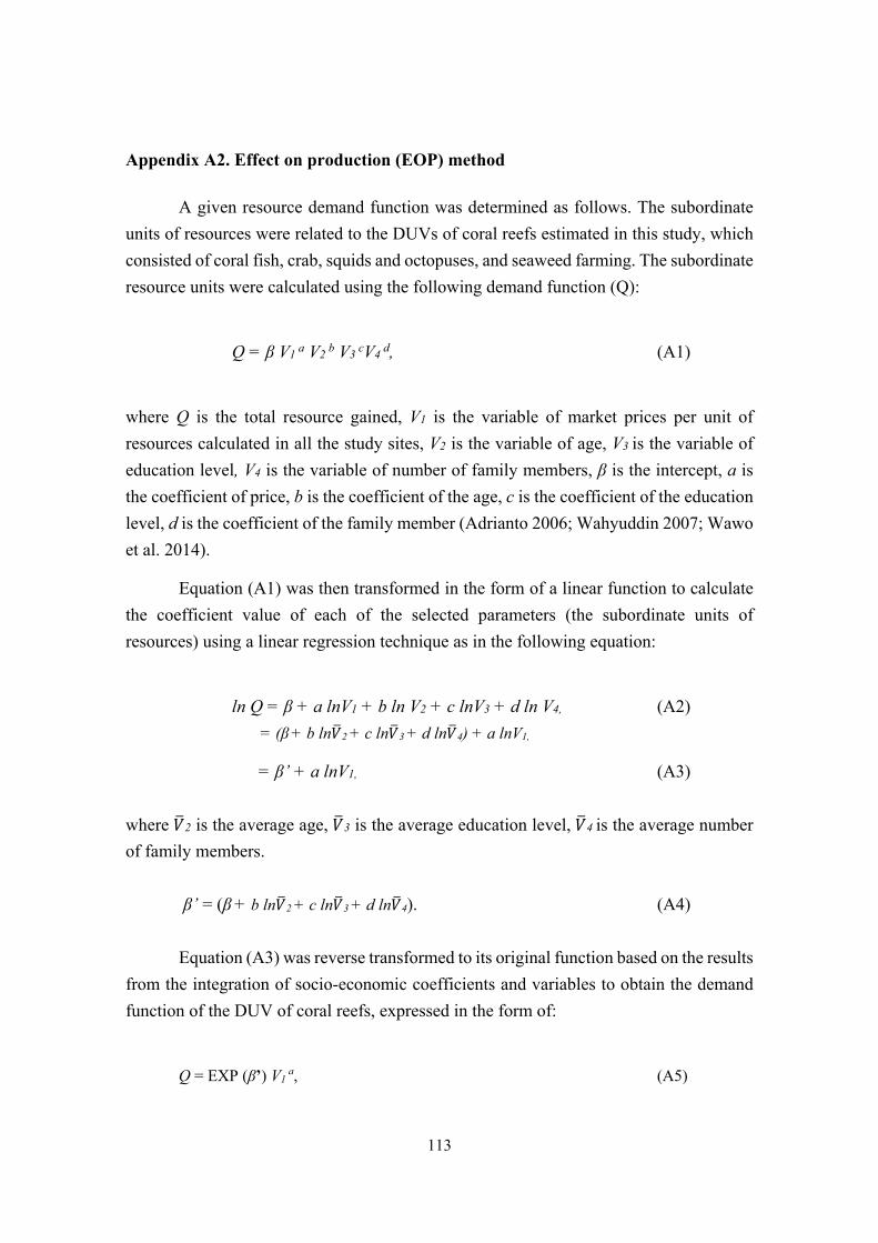
113
Appendix A2. Effect on production (EOP) method
A given resource demand function was determined as follows. The subordinate
units of resources were related to the DUVs of coral reefs estimated in this study, which
consisted of coral fish, crab, squids and octopuses, and seaweed farming. The subordinate
resource units were calculated using the following demand function (Q):
Q = β V1 a V2
b V3 cV4
d, (A1)
where Q is the total resource gained, V1 is the variable of market prices per unit of
resources calculated in all the study sites, V2 is the variable of age, V3 is the variable of
education level, V4 is the variable of number of family members, β is the intercept, a is
the coefficient of price, b is the coefficient of the age, c is the coefficient of the education
level, d is the coefficient of the family member (Adrianto 2006; Wahyuddin 2007; Wawo
et al. 2014).
Equation (A1) was then transformed in the form of a linear function to calculate
the coefficient value of each of the selected parameters (the subordinate units of
resources) using a linear regression technique as in the following equation:
ln Q = β + a lnV1 + b ln V2 + c lnV3 + d ln V4, (A2)
= (β + b ln 2 + c ln 3 + d ln 4) + a lnV1,
= β’ + a lnV1, (A3)
where 2 is the average age, 3 is the average education level, 4 is the average number
of family members.
β’ = (β + b ln 2 + c ln 3 + d ln 4). (A4)
Equation (A3) was reverse transformed to its original function based on the results
from the integration of socio-economic coefficients and variables to obtain the demand
function of the DUV of coral reefs, expressed in the form of:
Q = EXP (β’) V1 a, (A5)
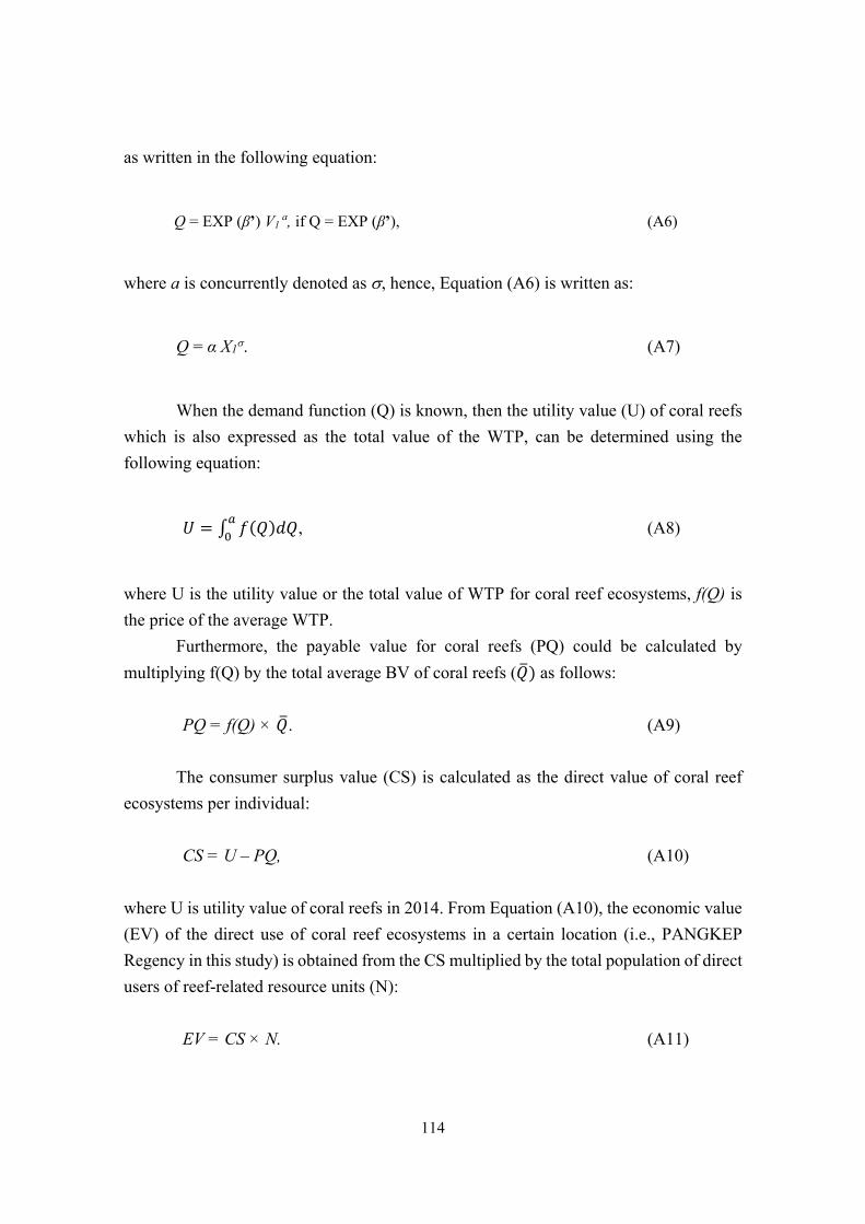
114
as written in the following equation:
Q = EXP (β’) V1 a, if Q = EXP (β’), (A6)
where a is concurrently denoted as , hence, Equation (A6) is written as:
Q = α X1. (A7)
When the demand function (Q) is known, then the utility value (U) of coral reefs
which is also expressed as the total value of the WTP, can be determined using the
following equation:
, (A8)
where U is the utility value or the total value of WTP for coral reef ecosystems, f(Q) is
the price of the average WTP.
Furthermore, the payable value for coral reefs (PQ) could be calculated by
multiplying f(Q) by the total average BV of coral reefs ( as follows:
PQ = f(Q) × . (A9)
The consumer surplus value (CS) is calculated as the direct value of coral reef
ecosystems per individual:
CS = U – PQ, (A10)
where U is utility value of coral reefs in 2014. From Equation (A10), the economic value
(EV) of the direct use of coral reef ecosystems in a certain location (i.e., PANGKEP
Regency in this study) is obtained from the CS multiplied by the total population of direct
users of reef-related resource units (N):
EV = CS × N. (A11)
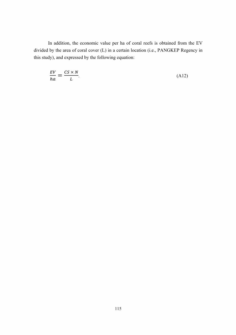
115
In addition, the economic value per ha of coral reefs is obtained from the EV
divided by the area of coral cover (L) in a certain location (i.e., PANGKEP Regency in
this study), and expressed by the following equation:
. (A12)
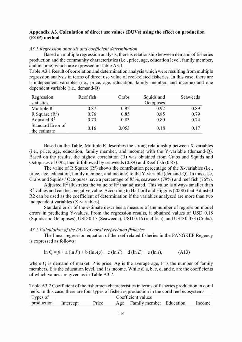
116
Appendix A3. Calculation of direct use values (DUVs) using the effect on production (EOP) method A3.1 Regression analysis and coefficient determination
Based on multiple regression analysis, there is relationship between demand of fisheries production and the community characteristics (i.e., price, age, education level, family member, and income) which are expressed in Table A3.1. Table A3.1 Result of correlation and determination analysis which were resulting from multiple regression analysis in terms of direct use value of reef-related fisheries. In this case, there are 5 independent variables (i.e., price, age, education, family member, and income) and one dependent variable (i.e., demand-Q)
Regression statistics
Reef fish Crabs Squids and Octopuses
Seaweeds
Multiple R 0.87 0.92 0.92 0.89R Square (R2) 0.76 0.85 0.85 0.79Adjusted R2 0.73 0.83 0.80 0.74Standard Error of the estimate
0.16 0.053 0.18 0.17
Based on the Table, Multiple R describes the strong relationship between X-variables (i.e., price, age, education, family member, and income) with the Y-variable (demand-Q). Based on the results, the highest correlation (R) was obtained from Crabs and Squids and Octopuses of 0.92, then it followed by seaweeds (0.89) and Reef fish (0.87).
The value of R Square (R2) shows the contribution percentage of the X-variables (i.e., price, age, education, family member, and income) to the Y-variable (demand-Q). In this case, Crabs and Squids / Octopuses have a percentage of 85%, seaweeds (79%) and reef fish (76%).
Adjusted R2 illustrates the value of R2 that adjusted. This value is always smaller than R2 values and can be a negative value. According to Harbord and Higgins (2008) that Adjusted R2 can be used as the coefficient of determination if the variables analyzed are more than two independent variables (X-variables).
Standard error of the estimate describes a measure of the number of regression model errors in predicting Y-values. From the regression results, it obtained values of USD 0.18 (Squids and Octopuses), USD 0.17 (Seaweeds), USD 0.16 (reef fish), and USD 0.053 (Crabs).
A3.2 Calculation of the DUV of coral reef-related fisheries
The linear regression equation of the reef-related fisheries in the PANGKEP Regency is expressed as follows:
ln Q = β + a (ln P) + b (ln Ag) + c (ln F) + d (ln E) + e (ln I), (A13) where Q is demand of market, P is price, Ag is the average age, F is the number of family members, E is the education level, and I is income. While β, a, b, c, d, and e, are the coefficients of which values are given as in Table A3.2. Table A3.2 Coefficient of the fishermen characteristics in terms of fisheries production in coral reefs. In this case, there are four types of fisheries production in the coral reef ecosystems. Types of production
Coefficient values Intercept Price Age Family member Education Income

117
(β) (a) (b) (c) (d) (e)Reef fish 26.18 -1.91 -0.13 0.19 -0.15 0.00Crabs 25.38 -1.86 0.01 0.01 -0.003 0.00Squids and Octopuses
27.21 -1.77 -0.75 -0.04 0.28 0.00
Seaweeds 14.47 -1.54 -0.67 0.10 0.0002 0.72
If the coefficients obtained by the regression analysis (Table A3.2) are substituted into Equation (A13), it is modified in the following:
a. Fish coral: ln Q = 25.96 – 1.91 (ln P), (A14)
b. Crabs: ln Q = 25.40 – 1.86 (ln P), (A15)
c. Squids and Octopuses: ln Q = 26.69 – 1.77 (ln P), (A16)
d. Seaweeds: ln Q = 14.64 – 1.54 (ln P). (A17)
Then function A14 through A17 were transformed into a non-linear equation as follows:
a. Coral Fish: Q = 188601317946.42 P -1.91, (A18)
b. Crabs: Q = 11433584409.38 P -1.86, (A19)
c. Squids and Octopuses: Q = 41616852299.79 P -1.77, (A20)
d. Seaweeds: Q = 9492363691.66 P -1.54. (A21)
To facilitate the estimation of some component values in effect on production (EOP) methods in terms of utilities, average WTP, debt values, and consumer surplus, then this study was used Maple software. Maple is math software that combines the world's most powerful math engine with an interface that makes it extremely easy to analyze, explore, visualize, and solve mathematical problems (Maple 2015). By using Maple Software, the function A18 through A21 can be formulated using the following equation:
a. Reef fish:
.. , (A22)
b. Crabs:
.. , (A23)
c. Squids and Octopuses:
.. , (A24)
d. Seaweeds:
.. . (A25)
Furthermore, from the function A22 through A25, several values as shown in Table A3.3 were obtained.
Table A3.3 The result of calculation of some component of value in the EOP method Types of Utility Average Payable Consumer
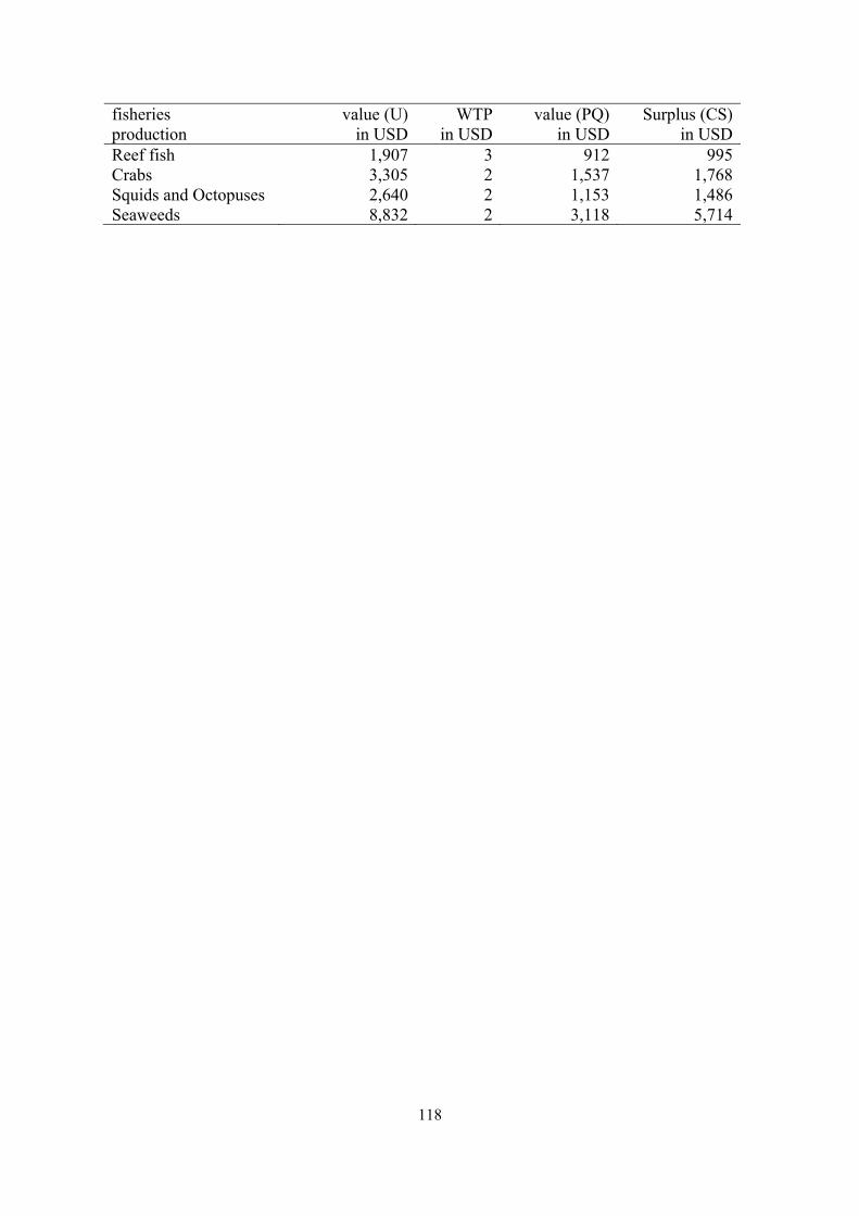
118
fisheries production
value (U) in USD
WTP in USD
value (PQ) in USD
Surplus (CS) in USD
Reef fish 1,907 3 912 995Crabs 3,305 2 1,537 1,768Squids and Octopuses 2,640 2 1,153 1,486Seaweeds 8,832 2 3,118 5,714
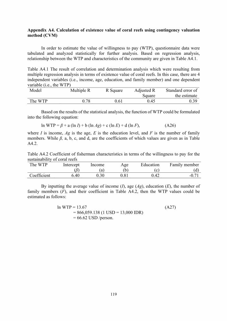
119
Appendix A4. Calculation of existence value of coral reefs using contingency valuation method (CVM)
In order to estimate the value of willingness to pay (WTP), questionnaire data were tabulated and analyzed statistically for further analysis. Based on regression analysis, relationship between the WTP and characteristics of the community are given in Table A4.1.
Table A4.1 The result of correlation and determination analysis which were resulting from multiple regression analysis in terms of existence value of coral reefs. In this case, there are 4 independent variables (i.e., income, age, education, and family member) and one dependent variable (i.e., the WTP) Model Multiple R R Square Adjusted R
SquareStandard error of
the estimateThe WTP 0.78 0.61 0.45 0.39
Based on the results of the statistical analysis, the function of WTP could be formulated
into the following equation:
ln WTP = β + a (ln I) + b (ln Ag) + c (ln E) + d (ln F), (A26)
where I is income, Ag is the age, E is the education level, and F is the number of family members. While β, a, b, c, and d, are the coefficients of which values are given as in Table A4.2. Table A4.2 Coefficient of fisherman characteristics in terms of the willingness to pay for the sustainability of coral reefs The WTP Intercept
(β) Income
(a)Age(b)
Education(c)
Family member(d)
Coefficient 6.40 0.30 0.81 0.42 -0.71
By inputting the average value of income (I), age (Ag), education (E), the number of family members (F), and their coefficient in Table A4.2, then the WTP values could be estimated as follows:
ln WTP = 13.67 (A27) = 866,059.138 (1 USD = 13,000 IDR)
= 66.62 USD /person.