Timing  calibra,on  and    Radio  wavefront  shape    of  cosmic  ray  air  showers  

Arthur  Corstanje  Radboud  University  Nijmegen  

for  the  LOFAR  Key  Science  Project  Cosmic  Rays      

LOFAR  Community  Science  Workshop,    June  2,  2015  

Radio pulses from cosmic rays Short (10 ns) pulses from cosmic-ray particles > ~ 1017 eV In 200 - 400 LOFAR antennas on the ground, we measure: •  Lateral distribution of

•  Signal power (Nelles et al., 2014) •  Signal arrival time (Corstanje et al., 2015)

Ø  Wavefront shape •  Spectrum / pulse shape (Rossetto et al., in prep.) •  Polarization (Schellart et al., 2014)

•  Wavefront shape measurements

Arrival times for a cosmic ray Measuring arrival time of pulse in individual antennas:

•  Time series signal Apply Hilbert transform to get Hilbert envelope •  Envelope maximum is ‘the arrival time’

ns < 5 ns!

Time (µs)

Am

plitu

de

σ t =12.7SNR

Arrival times after subtracting plane-wave solution

Corstanje et al., Astropart. Phys. (2015)

Ground plane

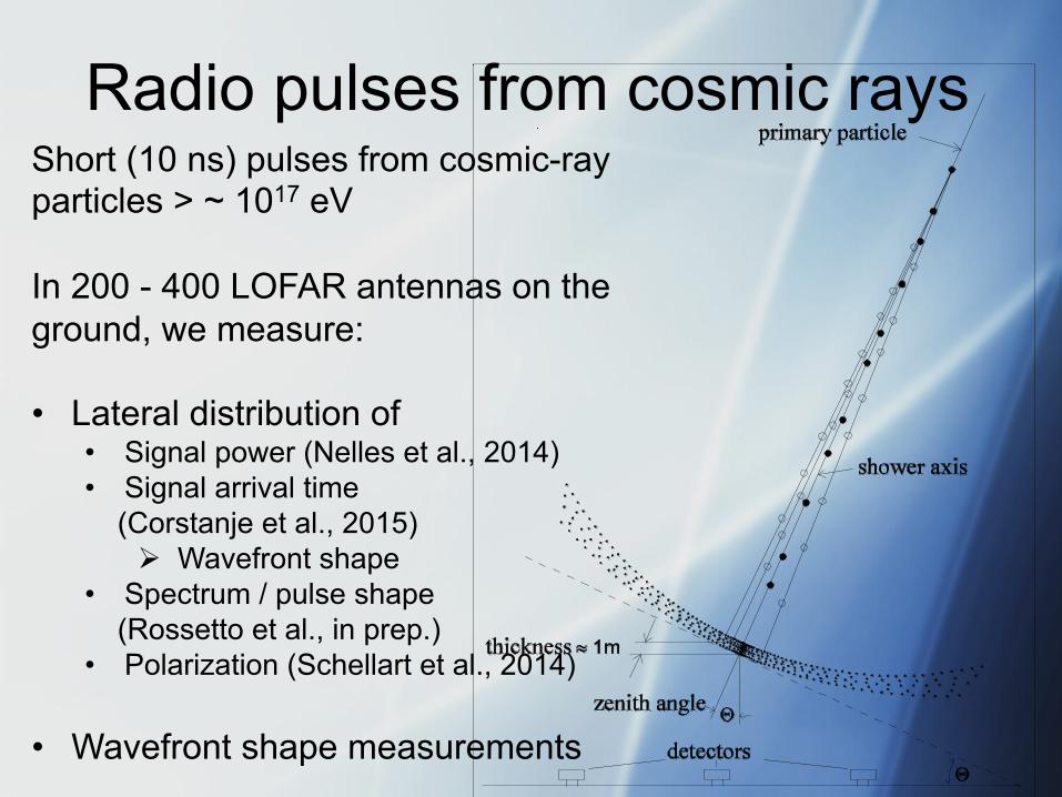
Shower  plane  projec,on  

∧ ∧ ∧ Shower core

Shower plane •  Project antennas into shower plane

•  Shower axis position: fixed using power-LDF (parametrization by Nelles et al., 2014)

•  Shower axis direction unknown to desired accuracy: free fit parameters

•  Wavefront: arrival times as function of distance from shower axis

•  Nested fitting (5 parameters): •  Optimize shower axis direction (2)

•  Optimize curve-fit (3)

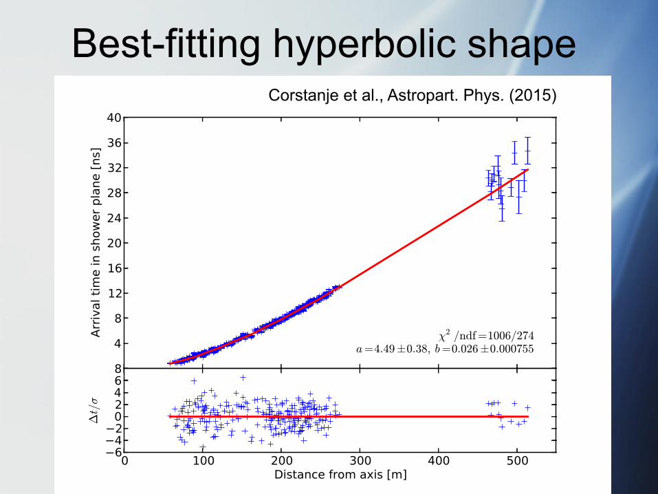
Best-fitting hyperbolic shape Corstanje et al., Astropart. Phys. (2015)

Another example

Conical-shaped example

Improved angular resolution

•  Using hyperbolic wavefront improves directional accuracy

•  About 1 degree

difference

•  Difference with conical shape

~ 0.1 degree

Tim

e la

g at

100

m [

ns ]

Corstanje et al., Astropart. Phys. (2015)

Comparing with simulations

•  Monte Carlo simulations of particles and radio emission, CoREAS.

•  25 proton showers, 15 iron showers •  Do pulse timing in the same way, in a 30 - 80 MHz bandpass window •  Look at wavefronts, processed from pulse

times with the same code

Proton simulations vs LOFAR data

Measured wavefront is steeper than any of the simulations! Uncertainty from core position is negligible

Iron simulations vs LOFAR data

Same deviation Cause? Antenna or filter characteristics? Or gap in understanding radio emission? èAlternative timing method cancels out dispersion

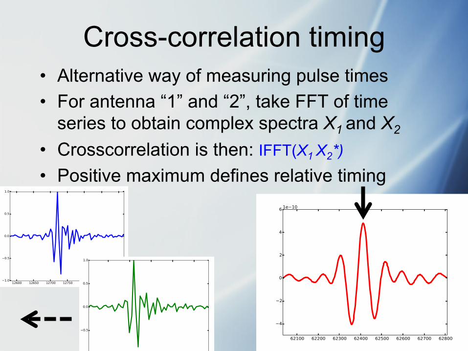
Cross-correlation timing •  Alternative way of measuring pulse times •  For antenna “1” and “2”, take FFT of time

series to obtain complex spectra X1 and X2 •  Crosscorrelation is then: IFFT(X1 X2*)

•  Positive maximum defines relative timing

Comparing timing methods

Hilbert envelope timing Cross-correlation timing

•  Wavefronts steeper with cross-correlation timing •  Both measured and simulated wavefronts

PRELIMINARY! | 250 m

-- 10 ns

Timing calibration using radio transmitter phases

•  Use phases of narrowband radio signals from a known transmitter (Smilde)

•  Relative phases per baseline from FFT of time series •  average over ~ 50 blocks of 8000 samples (2 ms!) •  Compare measured phases with calculated phases from

source position •  Use GPS location converted to ITRF

•  Gives calibration delays per antenna pair, modulo ~ 11 ns for each frequency

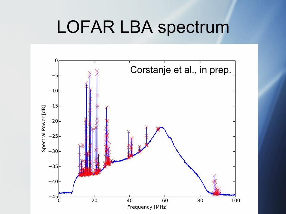
LOFAR LBA spectrum

Corstanje et al., in prep.

Calibration timing signal per antenna (one polarization)

Stable calibration Small diff wrt Caltables Sigma ~ 0.4 ns (per station) Ø  Includes all

systematics! Median gives inter- station clock offset

A. Corstanje et al.

Corstanje et al., in prep.

Differential measurements -  Measuring at the edge of the band (filter) and a signal

coming from the horizon -  Signal propagation effects not completely known +  Phase difference between channels takes out the

common filter characteristic at this frequency +  Given a starting (cross)calibration, e.g. astronomical: can

take difference between observations to observe trends, drifting, glitches etc.

Calibration timing offsets per antenna: variations over time

Mostly stable calibration Timing variations up to +/- 0.3 ns Sigma ~ 0.08 ns in a 24-hr bin (>= 5 data points)

A. Corstanje et al. Corstanje et al., in prep.

-- 1.0 ns

-- 0

Calibration timing signal per antenna: variations over time

Slow drifting, About 0.6 ns peak-peak Sigma ~ 0.08 ns in a 24-hr bin (>= 5 data points)

A. Corstanje et al. Corstanje et al., in prep.

-- 0.5 ns

-- 0 ns

| 50 days |

Conclusions and outlook •  Wavefront timing measured with accuracy better than 1 ns per antenna for strong showers •  A hyperboloid fits best; no structure in residuals •  Simulation comparison shows that measured

wavefronts are steeper, cause unknown •  Cross-correlation timing: mismatch still there, but rules out phase component of filters (dispersion)

•  Timing calibration using FM radio works well, sigma ~ 0.4 ns per antenna, ~ 0.1 ns inter-station •  Only 2 ms of data, piggybacked, a few minutes end-to-end, radio signal always present •  Monitoring clock drifts with sigma ~ 0.08 ns

5 ns glitch…

~ Dec 14, 2014