Time-Variant Strength Capacity Model for GFRP BarsEmbedded in Concrete

Paolo Gardoni1; David Trejo, A.M.ASCE2; and Young Hoon Kim, A.M.ASCE3

Abstract: Glass fiber-reinforced polymer (GFRP) concrete reinforcement exhibits high strength, is lightweight, can decrease time of construc-tion, and is corrosion resistant. However, research has shown that chemical reactions deteriorate the GFRP reinforcing bars over time, resultingin a reduced tensile capacity. This paper develops a time-variant probabilistic model to predict the tensile capacity of GFRP bars embedded inconcrete. The developedmodel is probabilistic to properly account for the relevant sources of uncertainties, including the statistical uncertaintyin the estimation of the unknown model parameters (because of the finite sample size), the model error associated with the inexact model form(e.g., a linear expression is used when the actual and unknown relations are nonlinear), and missing variables (i.e., the model only includesa subset of the variables that influence the quantity of interest.) The proposed model is based on a general diffusion model, in which wateror ions penetrate the GFRP bar matrix and degrade the glass fiber-resin interface. Themodel indicates that GFRP reinforcement bars with largerdiameters exhibit lower rates of capacity loss. The proposed probabilistic model is used to assess the probability of not meeting the tensilestrength requirement based on specifications over time and can be used to assess the safety and performance of GFRP reinforced systems.Sensitivity and importance analyses are carried out to explore the effect of the parameters and random variables on the probability estimates.DOI: 10.1061/(ASCE)EM.1943-7889.0000588. © 2013 American Society of Civil Engineers.

CE Database subject headings: Bars; Glass fiber; Fiber reinforced polymers; Tensile strength; Deterioration; Reinforced concrete.

Author keywords: Glass fiber; Fiber-reinforced polymers; Tensile strength; Deterioration.

Introduction

Glass fiber-reinforced polymer (GFRP) reinforcement is being usedas reinforcement for concrete structures. Significant research hasbeen performed on this material (Vijay and Gangarao 1999; Dejke2001; Micelli et al. 2001; Almusallam et al. 2002; Giernacky et al.2002; Svecova et al. 2002; Micelli and Nanni 2004; Mukherjee andArwikar 2005; Bakis et al. 2005; Mufti et al. 2007a,b; Cain 2008;Huang and Aboutaha 2010). GFRP reinforcement has many ad-vantages over conventional steel reinforcement; it is lightweight,has a high strength-to-weight ratio, and the chemical or electro-chemical reactions between the environment and the GFRP do notresult in products with increased volumes that might result in concretecracking and spalling (Bradberry 2001).However, Trejo et al. (2005;2011) evaluated the potential use of GFRP reinforcement for bridgedecks and reported experimental results that indicated tensilestrength loss over time. In particular, Trejo et al. (2011) reportedexperimental tension test data for 160 GFRP reinforcement barsembedded in concrete and exposed to actual environmental con-ditions [mean annual temperature of 23�C (73�F) and average annual

precipitation of rain of 1,008 mm (39.7 in.)] for 7 years. The ex-perimental program included the assessment of two GFRP bar sizes,16 and 19 mm (5/8 and 3/4 in.) from three manufacturers. Although7 years of exposure is shorter than the typical service time of concretestructures, it is the longest exposure time for which data are currentlyavailable.

This paper develops a state-of-the-art, time-variant deteriorationmodel for GFRP reinforcing bars embedded in concrete. Unknownmodel parameters are calibrated using experimental data fromTrejo et al. (2011) and 27 additional data available in the literatureon GFRP reinforcement embedded in concrete (Tannous andSaadatmanesh 1998; Dejke 2001). Themodel is developed based ongeneral diffusion transport principles and predicts the residual ca-pacity of GFRP bars embedded in concrete. The developed model isprobabilistic and properly accounts for the relevant sources of in-formation, including the principles of diffusion transport and ex-perimental data. The model also accounts for uncertainties, includingthe statistical uncertainty in the estimation of the unknown modelparameters and the model error associated with the inexact modelform (e.g., a linear expression is used when the actual and unknownrelations are nonlinear) and missing variables (i.e., the model onlyincludes a subset of the variables that influence the quantity ofinterest.) The model shows that the residual tensile strength capacityis a function of time of embedment in concrete, t, the diffusioncoefficient of the GFRP polymer matrix, DT , and the GFRP barradius, r. In particular, the model predicts that GFRP reinforcementwith smaller diameters exhibit faster reductions in residual tensilestrength than larger diameter GFRP reinforcing bars.

The developed time-variant model provides the required in-formation to assess the safety and performance of GFRP reinforcingbars embedded in decks, pavements, and other infrastructure ele-ments over time. In this paper, the proposed probabilistic model isused to assess the probability of not meeting the tensile strengthrequirement over time and at different ambient temperatures, T . The

1Associate Professor, Dept. of Civil and Environmental Engineering,Univ. of Illinois at Urbana-Champaign, Urbana, IL 61801 (correspondingauthor). E-mail: gardoni@illinois.edu

2Professor and Construction Education Foundation Endowed Chair,School of Civil and Construction Engineering, Oregon State Univ., Cor-vallis, OR 97331.

3Assistant Professor, Dept. of Civil and Environmental Engineering,Univ. of Louisville, Louisville, KY 40292.

Note. This manuscript was submitted on January 12, 2011; approved onDecember 18, 2012; published online on December 21, 2012. Discussionperiod open until March 1, 2014; separate discussions must be submittedfor individual papers. This paper is part of the Journal of EngineeringMechanics, Vol. 139, No. 10, October 1, 2013. ©ASCE, ISSN 0733-9399/2013/10-1435–1445/$25.00.

JOURNAL OF ENGINEERING MECHANICS © ASCE / OCTOBER 2013 / 1435

J. Eng. Mech., 2013, 139(10): 1435-1445

Dow

nloa

ded

from

asc

elib

rary

.org

by

OR

EG

ON

ST

AT

E U

NIV

ER

SIT

Y o

n 03

/10/

17. C

opyr

ight

ASC

E. F

or p

erso

nal u

se o

nly;

all

righ

ts r

eser

ved.

first-order reliability method (FORM) and Monte Carlo (MC)simulations are used to assess estimates of this probability, alongwith confidence bounds, to implicitly or explicitly reflect the in-fluence of the epistemic uncertainties. Sensitivity and importanceanalyses are carried out to explore the effect of changes in theparameters and randomvariables on the probability estimates. Basedon the results of the importance analysis, an approximate closed formof the probability of not meeting the tensile strength requirement isalso proposed.

This paper first discusses the deterministic models currentlyavailable in the literature to predict the tensile strength capacity ofGFRP bars. Next, the minimum design requirements according toAmerican Concrete Institute (ACI) Committee 440.1R (ACI 2007)are reviewed. The following section formulates the probabilisticcapacity model, which is then calibrated in the following sectionusing experimental data. The probability of not meeting the ACIdesign requirement is then estimated and the sensitivity and im-portance analyses are carried out. Finally, the approximate closedform to estimate the probability of not meeting the design re-quirements is proposed.

Models from the Literature

The constituent materials of GFRP bars and their exposure con-ditions play a significant role in the performance of GFRP bars.Deterministic models have been developed to predict the residualstrengths at different times, thereby providing the designer with pos-sible estimates of bar capacity at later ages. These residual strengths, orfactored residual strengths, could then be used in the design ofGFRPRC elements. This section provides a review of the available modelsfor assessing the residual strength of GFRP bars embedded in con-crete. Two limitations common to all the available models are that(1) only limited long-term data on the performance of GFRP barsembedded in concrete were used (most data are for accelerated ex-posure conditions, and the exposure periods were less than threeyears), and (2) the models are typically biased and deterministic(i.e., they tend to be implicitly conservative and do not account forthe uncertainties inherent in the problem), and therefore, they pro-vide limited value for assessing the reliability or safety of concretestructures reinforced with GFRP bars.

The rate of diffusion of elements or compounds (e.g., water, al-kalis, and hydroxyl ions) has a significant impact on the residualstrength ofGFRPbars. Simply, the compounds are transported to theglass fibers where they react with the glass and debond the glassfibers from the resin composite. This results in a reduced residualstrength of GFRP bars, particularly, the tension. Therefore, Katsukiand Uomoto (1995) proposed a predictive model based on Fick’sfirst law. The authors assumed that the tensile strength of GFRP barscan be determined quantitatively by the amount of alkali penetrationarea into the bars and recommended that the depth of penetration canbe calculated using the following equation:

X ¼ffiffiffiffiffiffiffiffiffiffiffiffiffiffiffiffiffiffiffiffiffiffi2 ×DT ×C × t

p(1)

where X 5 depth of penetration from the surface; DT 5 diffusioncoefficient at temperature T ; C 5 alkaline concentration (percent);and t is the curing time. Various units can be used in this equation, andthe units of the square root of the product should result in a length unit.

Katsuki and Uomoto (1995) assumed that, as the glass fibers areexposed to a diffusing solution, the fibers exhibit complete failureand no longer contribute to the bars’ load bearing capacity. Theauthors then proposed the following equation for estimating theresidual strength:

st ¼�12

ffiffiffiffiffiffiffiffiffiffiffiffiffiffiffiffiffiffiffiffiffiffi2 ×DT ×C × t

pr

�2

×s0 (2)

wheres0 andst 5 tensile strengths before and after exposure (stressunits), respectively. A similar approach was proposed by Tannousand Saadatmanesh (1998).

Trejo et al. (2005) reported that the assumption of complete lossof glass fiber capacity upon immediate contact with the solutionlikely overestimated the loss of capacity and proposed an exposurefactor, l, to account for this time-dependent deterioration of thebond between the glass and resin. The formula, modified with theexposure factor, is as follows:

st ¼�12

ffiffiffiffiffiffiffiffiffiffiffiffiffiffiffiffiffiffiffiffiffiffi2 ×DT × l × t

pr

�2

×s0 (3)

where the definitions of the variables have already been reported,andl is amodel parameter that typically varieswith the solution typeand exposure time.

Because the rate of chemical reactions is dependent on temper-ature, it would be beneficial to consider the influence of tempera-ture on tensile strength capacity. The Arrhenius equation has beenwidely used to establish relationships between degradation data fromlaboratory-accelerated aging tests and service life of field structures.Proctor et al. (1982) suggested that time–temperature relationshipscan be obtained using deterioration data of material after exposurein concrete at different temperatures. If the shape of the residualstrength curves is a function of the logarithmof time and is similar fordifferent temperatures, the Arrhenius equation could be applicable.Katsuki and Uomoto (1995) reported that the Arrhenius equationoffers a good correlation between the temperature and the rate ofdiffusivity and chemical reactions. The Arrhenius equation is shownas follows:

kr ¼ Ae2Ea=RT (4)

where kr 5 the rate constant; A 5 the frequency factor; Ea 5 theactivation energy (kilojoules); R 5 the universal gas constant(kilojoules per molar 3 kelvins); and T5 the absolute temperature(kelvins).

Eq. (4) can also be used to determine the influence of temperatureon the diffusion coefficient,DT , by substituting kr withDT as follows:

DT ¼ Ae2Ea=RT (5)

Eq. (5) can then be used to determine the relative change in diffusionrates as follows:

DT

DT , ref¼ A × e2Ea=RT

A × e2Ea=RTref¼ eEa=Rð1=Tref21=TÞ (6)

where T and Tref 5 exposure temperatures (in kelvins). Assumingdata on capacity loss can be generated at some reference temper-ature, Tref , an estimate on the capacity loss of GFRP bars at a dif-ferent temperature can be determined by including Eq. (6) intoEq. (3) as follows:

st ¼

2412

ffiffiffiffiffiffiffiffiffiffiffiffiffiffiffiffiffiffiffiffiffiffiffiffiffiffiffiffiffiffiffiffiffiffiffiffiffiffiffiffiffiffiffiffiffiffiffiffiffiffiffiffiffiffiffiffiffiffiffiffiffi2 ×DT , ref × e

Ea=Rð1=Tref21=TÞ × l × tq

r

352

×s0 (7)

Note that atT5 Tref , the exponential term goes to unity, and Eqs. (3)and (7) are the same. Therefore, by determining the capacity loss of

1436 / JOURNAL OF ENGINEERING MECHANICS © ASCE / OCTOBER 2013

J. Eng. Mech., 2013, 139(10): 1435-1445

Dow

nloa

ded

from

asc

elib

rary

.org

by

OR

EG

ON

ST

AT

E U

NIV

ER

SIT

Y o

n 03

/10/

17. C

opyr

ight

ASC

E. F

or p

erso

nal u

se o

nly;

all

righ

ts r

eser

ved.

GFRP bars at a reference temperature, information can be generatedon the performance of GFRP bars at other temperatures. Acceleratedshort-term tests indicate that the activation energy is significantlyinfluenced by the chemical composition of the GFRP bar and poresolution of the concrete (Chen et al. 2006). In addition, short-termaccelerated tests can lead to high uncertainty of the activationenergy value for the GFRP bars exposed to high pH pore solutions(Chin et al. 2001; Chen et al. 2006). Yu et al. (2007) also reportedthat the determination of parameters in the Arrhenius law were alsohighly uncertain. Because determining the exact value of these pa-rameters is beyond the scope of this paper, the activation energy isassumed to be the average value of Proctor’s extensive data set(range, 89–93 kJ/mol). The data set is not from the GFRP barsembedded in concrete, but the data set is considered to be reasonablefor the degradation of glass fibers in cementitious materials for long-term exposure.

The literature indicates that the loss of GFRP bar capacity isa result of water or alkaline solution diffusing through the polymer tothe glass fiber–polymer interface, resulting in deterioration of theglass fiber, which results in debonding of the glass fiber from thepolymer.As thewater or solution continues to penetrate the polymer,more glass fibers are debonded, resulting in further reduction incapacity.

Tensile Strength Design Requirements

ACI Committee 440.1R (ACI 2007) and AASHTO Load and Re-sistance Factor Design (AASHTO 2008) specifications require useof an environmental reduction factor as a design parameter whenconsidering the reduction in tensile strength of GFRP in actualstructures. This reduction factor, CE, depends on the exposureconditions of the GFRP RC. For concrete not exposed to earth andweather, the reduction factor is 0.8, and for concrete exposed to earthand weather, the reduction factor is 0.7. The design tensile strength,ffu, of GFRP reinforcing bar considering these required reductionscan then be determined as follows:

ffu ¼ CEfpfu (8)

where f pfu 5 guaranteed ultimate tensile strength (GUTS) of a GFRPbar; andCE 5 environmental reduction factor equal to 0.8 for GFRPembedded in concrete not exposed to earth and weather and equal to0.7 for GFRP RC exposed to earth and weather. The GUTS isdefined as the mean tensile strength of a set of test specimens minusthree SDs ð f pfu 5 fu,ave 2 3sÞ.

Formulation of the Proposed ProbabilisticCapacity Model

By substituting Eq. (6) in Eq. (3) and replacing the square root withan unknown parameter a, the model in Eq. (3) based on Trejo et al.(2005) is modified into the following phenomenologic model:

st ¼(12 l

"DT , ref × e

Ea=Rð1=Tref21=TÞ × tr2

#a)×s0 (9)

where each term has the same definition as in Eq. (3), and a and lare two unknown model parameters used to fit the data. To accountfor the uncertainty in s0 and st, Eq. (9) is then modified as followsby addicting some variability in s0 and in the effects of thedeterioration:

stðx,QÞ ¼(ð1þ s0 × ɛ0Þ2 l

"DT , ref × e

Ea=Rð1=Tref21=TÞ × tr2

#a

� �1þ s × ɛ

�)×ms0

(10)

where x5 ðDT ,ref ,Ea,R, r,TÞ is a vector of basic variables(i.e., material properties, geometry, and temperature); s0 × ɛ0 5 anerror term that captures the variability of s0 around its mean ms0

;s × ɛ 5 an error term that captures the variability in the reductionterm lfDT ,ref ×exp½Ea=R×ð1=Tref21=TÞ�×t=r2ga; ɛ0 and ɛ 5 sta-tistically independent identically distributed random variables withzero mean and unit variance; s0 and s5 SDs of the two error terms;and Q5ðl,a,s0,sÞ is a vector of unknown model parameters. Twoassumptions are made in formulating the model: (1) s0 and s are notfunctions of x (homoskedasticity assumption), and (2) ɛ0 and ɛ havea normal distribution (normality assumption).Diagnostic plots of thedata and the residuals against model predictions (Rao and Tou-tenburg 1997) were used to verify the validity of these assumptions.The specific values of the parameters in Q depend on the values ofthe experimental data.

Based on the normality assumption, Eq. (10) can be rewritten as(Ang and Tang 2007)

stðx,QÞms0

¼(12l

"DT , ref × e

Ea=Rð1=Tref21=TÞ × tr2

#a)

þ

ffiffiffiffiffiffiffiffiffiffiffiffiffiffiffiffiffiffiffiffiffiffiffiffiffiffiffiffiffiffiffiffiffiffiffiffiffiffiffiffiffiffiffiffiffiffiffiffiffiffiffiffiffiffiffiffiffiffiffiffiffiffiffiffiffiffiffiffiffiffiffiffiffiffiffiffiffiffiffis20 þ l2

"DT , ref × e

Ea=Rð1=Tref21=TÞ × tr2

#2as2

vuut × ɛ

(11)

Eq. (11) is used in the next section to assess the model parametersQ using experimental data. Later, Eq. (11) is used to develop anapproximate estimate of the probability that the tensile strengthrequirement based on specifications is not met as a function of t, r,and T .

Model Assessment

The model in Eq. (11) is assessed using experimental data fromGFRP bars embedded in concrete for 7 years. A Bayesian approachis used to estimate the statistics (means, variances, and correlationcoefficients) of the unknown parameters (Box and Tiao 1991). ABayesian approach is particularly suitable because it allows updatingof the statistics of the unknown model parameters as new databecome available.

Experimental Data

Trejo et al. (2011) provided experimental data on the residual tensilestrength capacity of 160 GFRP bars with diameters of 16 and 19mm(5/8 and 3/4 in.) provided by three different manufacturers. Thebars contained approximately 70% of unidirectional glass fibers byvolume; the remaining volumes were resin, filler, and air voids.Three different bar types, P, V1, and V2, representing three man-ufacturers, were evaluated. It should be noted that the P bars are nolonger being produced. Table 1 provides a breakdown of the GFRPspecimens by bar type and size.

Schaefer (2002) reported that bar Type P was made with a po-lyethylene terephthalate (PET) polyester matrix and E-glass fibers.

JOURNAL OF ENGINEERING MECHANICS © ASCE / OCTOBER 2013 / 1437

J. Eng. Mech., 2013, 139(10): 1435-1445

Dow

nloa

ded

from

asc

elib

rary

.org

by

OR

EG

ON

ST

AT

E U

NIV

ER

SIT

Y o

n 03

/10/

17. C

opyr

ight

ASC

E. F

or p

erso

nal u

se o

nly;

all

righ

ts r

eser

ved.

Bar Type V1 contained E-glass fibers embedded in a vinyl esterresin. This bar was made with external helical fiber wrapping, andthe surface of the bar was coated with fine sand. Bar Type V2 wascomposed of E-glass fibers embedded in a vinyl ester resin and hada circular cross section coated with coarser sand. Trejo et al. (2005)measured and reported a range of diffusion coefficients for the differentGFRP bars evaluated at 23�C (73�F) to be from 2:883 10213 m2=s(4:473 10210 in:2=s) to 1:543 10212 m2=s (2:393 1029 in.2=s),with a mean value of 8:903 10213 m2=s (1:383 1029 in:2=s) anda standard deviation of 3:523 10213 m2=s (0:543 1029 in:2=s). Thestatistics of the diffusion coefficients are used for the modeling inthis paper.

GFRP RC samples were exposed for 7 years to outdoor envi-ronmental conditions with a mean annual temperature of 23�C(73�F) and a mean annual precipitation of 1,008 mm (39.7 in.), fairlyevenly distributed throughout the year. Theminimumandmaximumaverage daily temperatures were 5�C (41�F) and 40�C (104�F),respectively. In addition, bars not exposed to outdoor environmentalconditions are used in this paper as control specimens. Additionaldetails on the material characterization of these GFRP bars can befound in Trejo et al. (2011). Although 7 years of exposure is shorterthan the typical service life of concrete structures, it is the longestexposure time for which data are currently available.

Additional data on GFRP bar capacity were provided byTannous and Saadatmanesh (1998) and Dejke (2001). Tannous andSaadatmanesh (1998) provided experimental data obtained fromtension tests of 10 GFRP bars embedded in concrete for 1 and 2years. The GFRP specimens manufactured by Kodiak FRP Rebar(Dayton, Texas) and International Grating (Houston, Texas) wereconstructed from E-glass fibers, had a fiber volume fraction of 72%,and consisted of polyester and vinylester resin matrices. The bar sizewas 10 mm (3/8 in.).

Dejke (2001) reported the residual tensile properties of 17 GFRPbars of different diameters, 9 mm (0.354 in.) and 8 mm (0.315 in.),manufactured by Hughes Brothers (Seward, Nebraska) and Fiber-konst (Malmö, Sweden), respectively. GFRP specimens were em-bedded in concrete under different temperature conditions, 20�C(68�F) and 40�C (104�F), for approximately 1 year. The concretespecimens with GFRP bars embeddedwere stored outdoors at 100%humidity to simulate a real concrete structure under highly moistconditions. After the bars were extracted from the concrete, tensiontests were performed to assess the residual bar capacity.

Bayesian Parameter Estimation

The unknown parameters Q are estimated using the followingBayesian updating rule (Box andTiao 1991), which updates the stateof knowledge aboutQ available before the data are collected into annew state of knowledge aboutQ, which reflects bothwhatwas knownbefore the data are collected and the information from the data

f ðQÞ ¼ cLðQÞpðQÞ (12)

wherepðQÞ5 previous distribution ofQ based on knowledge aboutQ before observing the set of data D of size n5 187; LðQÞ5 likelihood function that represents the objective information onQ from D, which is proportional to the conditional probabilityPðD jQÞ of observing D for given values of Q; c 5 normalizingfactor; and f ðQÞ 5 posterior distribution of Q that incorporatesthe information in pðQÞ andD. The posterior mean vector,MQ, andthe covariancematrix,SQQ, are obtained once f ðQÞ is known. In theanalysis presented in this paper, a noninformative previous distri-bution is assumed to reflect that there is no or little informationavailable aboutQ before collectingD. If new data become availablein the future, Eq. (12) can also be used to update the estimates of themodel parameters using the current posterior distribution f ðQÞ asa new previous distribution.

For each data point i in D, the residual ri for i5 1, . . . , n iswritten as

ri�l,a

� ¼ st i

ms0 i2

(12 l

"DT ,ref × e

Ea=Rð1=Tref21=TÞ × tir2i

#a)(13)

The residual ri is the difference between the measured and the meanof the predicted normalize stressesst=ms0

. The residuals capture theaccuracy of the model in predicting the measured quantities. Themore accurate the model is, the smaller are the residuals. UsingEqs. (11) and (13), LðQÞ can be written as

L�Q� ¼ ∏

n

i¼1P

( ffiffiffiffiffiffiffiffiffiffiffiffiffiffiffiffiffiffiffiffiffiffiffiffiffiffiffiffiffiffiffiffiffiffiffiffiffiffiffiffiffiffiffiffiffiffiffiffiffiffiffiffiffiffiffiffiffiffiffiffiffiffiffiffiffiffiffiffiffiffiffiffiffiffiffiffiffiffiffis20 þ l2

"DT ,ref × e

Ea=Rð1=Tref21=TÞ × tir2i

#2as2

vuut × ɛi

¼ ri�l,a

�)

(14)

As defined earlier, LðQÞ is a measure of the probability of observingthe experimental data for given values ofQ. FollowingGardoni et al.(2002), because ɛ has the standard normal distribution, LðQÞ canbe rewritten using the standard normal probability density functionwð×Þ as

L�Q� ¼ ∏

n

i¼1

1ffiffiffiffiffiffiffiffiffiffiffiffiffiffiffiffiffiffiffiffiffiffiffiffiffiffiffiffiffiffiffiffiffiffiffiffiffiffiffiffiffiffiffiffiffiffiffiffiffiffiffiffiffiffiffiffiffiffiffiffiffiffiffiffiffiffiffiffiffiffiffiffiffiffiffiffiffiffiffis20 þ l2

"DT ,ref × e

Ea=Rð1=Tref21=TÞ × tir2i

#2as2

vuut

� w

8>>>><>>>>:

riðl,aÞffiffiffiffiffiffiffiffiffiffiffiffiffiffiffiffiffiffiffiffiffiffiffiffiffiffiffiffiffiffiffiffiffiffiffiffiffiffiffiffiffiffiffiffiffiffiffiffiffiffiffiffiffiffiffiffiffiffiffiffiffiffiffiffiffiffiffiffiffiffiffiffiffiffiffiffiffiffiffiffis20 þ l2

"DT , ref × e

Ea=Rð1=Tref21=TÞ × tir2i

#2as2

vuut

9>>>>=>>>>;(15)

where the term in the parentheses is the functional argument of wð×Þ.Table 2 lists the posterior statistics ofQ obtained using the data fromthe experimental program of this project and the additional dataavailable from the literature.

Table 1. Number of GFRP Specimens by Bar Type, Size, and NominalConcrete Cover [after Trejo et al. (2011)]

Bar typeNominal

diameter, mm (in.)25.4 mm

(1 in.) cover50.8 mm

(2 in.) cover76.2 mm

(3 in.) cover Total

V1 16 (5/8) 10 14 11 3519 (3/4) 9 10 10 29

V2 16 (5/8) 10 10 10 3019 (3/4) 8 5 5 18

P 16 (5/8) 5 5 5 1519 (3/4) 11 11 11 33

Total 47 45 45 160

1438 / JOURNAL OF ENGINEERING MECHANICS © ASCE / OCTOBER 2013

J. Eng. Mech., 2013, 139(10): 1435-1445

Dow

nloa

ded

from

asc

elib

rary

.org

by

OR

EG

ON

ST

AT

E U

NIV

ER

SIT

Y o

n 03

/10/

17. C

opyr

ight

ASC

E. F

or p

erso

nal u

se o

nly;

all

righ

ts r

eser

ved.

Fig. 1 shows a comparison between the predicted and measurednormalized tensile strength st=ms0

over time. The experimentaldata are shown as dots (•) for all bar types. The mean predictionðɛ0 5 ɛ5 0Þ is shown as a solid line [in the top plot for the 10-mm(3/8 in.) bars, in the center plot for the 16-mm (5/8 in.) bars, and inthe bottom plot for the 19-mm (3/4 in.) bars]. The dashed linesdelimit the region within one SD of the mean. In addition, thehorizontal dotted line represents the ACI 440 minimum capacityrequirement, ffu=ms0

5 0:595, where with reference to Eq. (8),ffu 5CEf pfu 5CEð fu,ave 2 3sÞ. An analysis of the data from the

experimental program and the additional data available from theliterature showed that s=ms0

varies between 0.02 and 0.09. For thepurpose of the analysis conducted in this section, the ACI re-quirement was computed using s=ms0

5 0:05. For each set of valuesof the input variables, themodel predicts only one value of the quantityof interest [i.e., Eðst=ms0

Þ]. In contrast, for the same set of inputvariables, multiple experimental outcomes are recorded. Such dif-ferences in the recorded outcomes can be attributed to differencesin other influencing variables that are not measured and are not in-cluded in the proposed model. The proposed probabilistic modeltells us what the expected value of the quantity of interest is for thegiven inputs and its variability around such an expected value to reflectthe fact that there is variability in the data. It can also be observedthat the decay of the mean normalized tensile capacity, Eðst=ms0

Þ, israpid over the first few years and gradually slows down as timeincreases. Furthermore, the decay is more pronounced for smaller barsthan for larger bars. Fig. 2 shows the values of t and r for whichEðst=ms0

Þ5CEð fu,ave 2 ksÞ=ms0for k5 3, . . . , 6 (k5 3 is the

value specified by ACI 440) at Tref . For small GFRP bar sizes,Eðst=ms0

Þst 5 ffu=ms0at a time less than the typical service life of

a structure. For small GFRP bar sizes, a larger value of k may berequired so thatEðst=ms0

Þ.CEð fu,ave 2 ksÞ=ms0during the service

time.

Probability of Not Meeting Design Specificationsover Time

Following the conventional notation in reliability theory (DitlevsenandMadsen 1996), a limit state function gð×Þ is introduced such thatthe event ½gð×Þ# 0� denotes not meeting a specified capacity re-quirement. In particular, the ACI 440 minimum capacity re-quirement, ffu, is considered.

Using the probabilistic model described in Eq. (11), a limit statefunction is written as

g�ffu, x, Q

� ¼ stðx,QÞ2 ffu (16)

Therefore, the probability of not meeting the design specifications atany time t is written as

PðQÞ ¼ Phg�ffu, x,Q

� # 0jQ

i(17)

where Pð× j ×Þ indicates the conditional probability of gð ffu, x,QÞ # 0for given values of Q.

Table 2. Posterior Statistics of the Unknown Parameters Q5 ðl,a, s0, sÞ

Parameter Mean SD

Correlation coefficient

l a s0 s

l 0.135 0.011 1a 0.207 0.082 20.84 1s0 0.039 0.003 20.04 0.04 1s 0.557 0.043 20.28 20.02 20.25 1

Fig. 1. Comparison between the predicted and measured normalizedstress st=ms0

over timeFig. 2. Values of t and r for which Eðst=ms0

Þ5CEð fu,ave 2 ksÞ=ms0

for k5 3, . . . , 6

JOURNAL OF ENGINEERING MECHANICS © ASCE / OCTOBER 2013 / 1439

J. Eng. Mech., 2013, 139(10): 1435-1445

Dow

nloa

ded

from

asc

elib

rary

.org

by

OR

EG

ON

ST

AT

E U

NIV

ER

SIT

Y o

n 03

/10/

17. C

opyr

ight

ASC

E. F

or p

erso

nal u

se o

nly;

all

righ

ts r

eser

ved.

The uncertainty in Eq. (17) arises from the inexact nature of themodel stðx,QÞ captured in ɛ0 and ɛ, the randomness in x, and theuncertainty in ffu. Table 3 lists the distributions and the corre-sponding statistics of the random variables in Eq. (17). Based on thenormality assumption already discussed, ɛ and ɛ0 follow a standardnormal distribution. For each of the other random variables, thedistributions are assumed based on the range of each variable (non-negative variables are assumed to follow a lognormal distribution),and the means and SDs are as provided in the references listed inTable 3.

Predictive Estimate

Following Gardoni et al. (2002), the predictive estimate of Eq. (17),~P, is defined as the expected value of PðQÞ over the distribution ofQ, f ðQÞ, that is

~P ¼ðQ

PðQÞf ðQÞ dQ (18)

By integrating overQ, the epistemic uncertainties are incorporatedinto the predictive estimates of the fragility in an average sense. Fur-thermore, the corresponding generalized reliability index (Ditlevsenand Madsen 1996) is obtained as

~b ¼ F21�12 ~P�

(19)

whereF21ð×Þ denotes the inverse of the standard normal cumulativedistribution function.

The probability of not meeting the ACI 440 design require-ments and the corresponding reliability index are functions of theinitial radius of a GFRP bar, r, (or its mean r) and time, t. Fig. 3shows a conceptual three-dimensional plot of the probability ofnot meeting the design requirements as a function of the radius ofa GFRP bar, r, and t. Consistent with the observations made forFig. 1, it can be seen that for a specified bar size, the probability ofnot meeting the design requirements increases with t. Con-versely, at the same t the probability decreases as the bar sizeincreases.

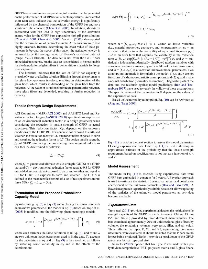
An analytical solution of Eq. (18) is typically not possible be-cause the analytical form for the integral is usually not available.Fig. 4 shows predictive estimates as a function of time computedusing MC simulations (Ditlevsen and Madsen 1996). The dottedline shows the probability for the 10-mm (3/8 in.) bars, thedashed line shows the probability for 16-mm (5/8 in.) bars, and thesolid line shows the probability for 19-mm (3/4 in.) bars. Con-sistent with the observations made from Fig. 1, in 75 years, 10-mm(3/8 in.) bars reach a 0.37 probability of not meeting the ACI 440

requirements, 16-mm (5/8 in.) bars reach a 0.23 probability, and19-mm (3/4 in.) bars reach a 0.18 probability. Note that the ex-posure temperature is assumed to be 23�C (73�F) in all figures,except for Fig. 5.

Fig. 5 shows the effect of exposure temperature on the proba-bilities estimated for 16-mm (5/8 in.) bars. The dotted line shows theprobability for the temperature of 33�C (91�F), the dashed lineshows the probability for the temperature (Tref ) of 23�C (73�F), andthe solid line shows the probability for the temperature of 13�C (55�F).As the exposure temperature increases, the probability also in-creases. In 75 years, at the exposure temperature of 13�C (55�F),16-mm (5/8 in.) bars reach a 0.09 probability, and at the exposuretemperature of 33�C (91�F), 16-mm (5/8 in.) bars reach a 0.37probability, which is 65% higher than a probability at the exposuretemperature of 23�C (73�F).

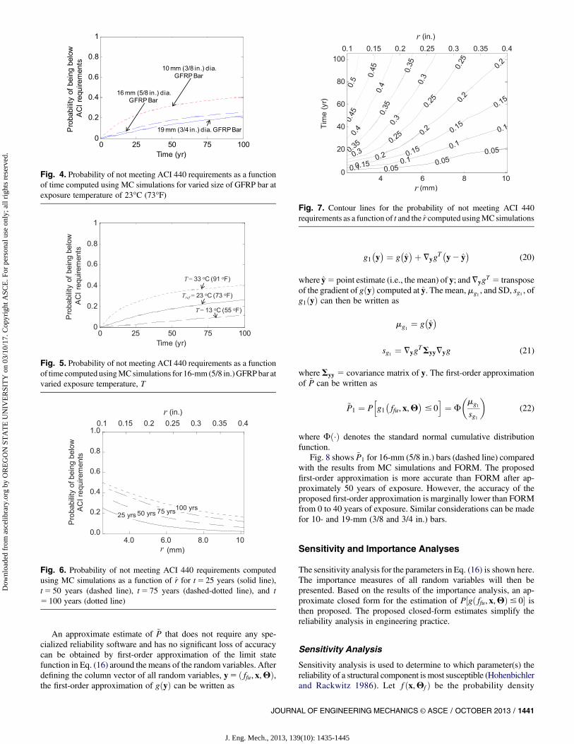
Fig. 6 shows the P½gð ffu, x,QÞ# 0� as a function of r. It can beseen that P½gð ffu, x,QÞ # 0� decreases as r increases and that theeffect of r is more pronounced shortly after the bars are embedded inconcrete than at later times. Finally, Fig. 7 shows a contour plot of theisoprobability lines for P½gð ffu, x,QÞ # 0� as a function of t and r.The isoprobability lines connect pairs of values of t and r thatcorrespond to the same P½gð ffu, x,QÞ # 0�. Consistent with whatwas observed in Figs. 4 and 6, Fig. 7 shows that P½gð ffu, x,QÞ # 0�increases as t increases, and that bars with larger r are less prone todeteriorate than bars with smaller r.

Fig. 8 shows a comparison between ~P for 16-mm (5/8 in.) barsestimated using MC simulations (shown as a line with open dots)and using the FORM (Ditlevsen andMadsen 1996) (shown as a solidline). Although results from MC simulations are in general moreaccurate than the ones from FORM, the latter also provides the ad-ditional sensitivity and importance measures described in the nextsection. The validity of the sensitivity and importance measures issupported by the match between the FORM and MC estimates.Similar considerations can be made for 10- and 19-mm (3/8 and3/4 in.) bars.

Table 3. Distributions and Corresponding Statistics of Random Variables

Random variablea Bar size Distribution Mean SD Reference/source

ffu=ms0Lognormal 0.595 0.060b Trejo et al. (2011)

DT ,ref , m2/s (in2/s) Lognormal 8:9033 10213

(1:373 1029)3:5223 10213

(5:453 10210)Trejo et al. (2005)

r, mm (in.) 10 mm (3/8 in.) Lognormal 4.5 (0.177) 0.56 (0.022) Kulkarni (2006)16 mm (5/8 in.) Lognormal 7.92 (0.312) 0.97 (0.038) Kulkarni (2006)19 mm (3/4 in.) Lognormal 0.375 (9.53) 1.14 (0.045) Kulkarni (2006)

ɛ, ɛ0 Normal 0 1 Normality assumptionaRandom variables are assumed to be statistically independent.bComputed assuming a 10% coefficient of variation.

Fig. 3. Conceptual plot of the probability of not meeting ACI 440requirements as a function of time and bar size

1440 / JOURNAL OF ENGINEERING MECHANICS © ASCE / OCTOBER 2013

J. Eng. Mech., 2013, 139(10): 1435-1445

Dow

nloa

ded

from

asc

elib

rary

.org

by

OR

EG

ON

ST

AT

E U

NIV

ER

SIT

Y o

n 03

/10/

17. C

opyr

ight

ASC

E. F

or p

erso

nal u

se o

nly;

all

righ

ts r

eser

ved.

An approximate estimate of ~P that does not require any spe-cialized reliability software and has no significant loss of accuracycan be obtained by first-order approximation of the limit statefunction in Eq. (16) around the means of the random variables. Afterdefining the column vector of all random variables, y5 ð ffu, x,QÞ,the first-order approximation of gðyÞ can be written as

g1�y� ¼ g

�y�þ =yg

T�y2 y�

(20)

where y5 point estimate (i.e., the mean) of y; and=ygT 5 transposeof the gradient of gðyÞ computed at y. The mean,mg1 , and SD, sg1 , ofg1ðyÞ can then be written as

mg1 ¼ g�y�

sg1 ¼ =ygTSyy=yg (21)

whereSyy 5 covariance matrix of y. The first-order approximationof ~P can be written as

~P1 ¼ Phg1�ffu, x,Q

� # 0

i¼ F

�mg1

sg1

�(22)

where Fð×Þ denotes the standard normal cumulative distributionfunction.

Fig. 8 shows ~P1 for 16-mm (5/8 in.) bars (dashed line) comparedwith the results from MC simulations and FORM. The proposedfirst-order approximation is more accurate than FORM after ap-proximately 50 years of exposure. However, the accuracy of theproposed first-order approximation is marginally lower than FORMfrom 0 to 40 years of exposure. Similar considerations can be madefor 10- and 19-mm (3/8 and 3/4 in.) bars.

Sensitivity and Importance Analyses

The sensitivity analysis for the parameters in Eq. (16) is shown here.The importance measures of all random variables will then bepresented. Based on the results of the importance analysis, an ap-proximate closed form for the estimation of P½gð ffu, x,QÞ # 0� isthen proposed. The proposed closed-form estimates simplify thereliability analysis in engineering practice.

Sensitivity Analysis

Sensitivity analysis is used to determine to which parameter(s) thereliability of a structural component is most susceptible (Hohenbichlerand Rackwitz 1986). Let f ðx,Qf Þ be the probability density

Fig. 4. Probability of not meeting ACI 440 requirements as a functionof time computed using MC simulations for varied size of GFRP bar atexposure temperature of 23�C (73�F)

Fig. 5. Probability of not meeting ACI 440 requirements as a functionof time computed usingMCsimulations for 16-mm (5/8 in.)GFRPbar atvaried exposure temperature, T

Fig. 6. Probability of not meeting ACI 440 requirements computedusing MC simulations as a function of r for t5 25 years (solid line),t5 50 years (dashed line), t5 75 years (dashed-dotted line), and t5 100 years (dotted line)

Fig. 7. Contour lines for the probability of not meeting ACI 440requirements as a function of t and the r computed usingMCsimulations

JOURNAL OF ENGINEERING MECHANICS © ASCE / OCTOBER 2013 / 1441

J. Eng. Mech., 2013, 139(10): 1435-1445

Dow

nloa

ded

from

asc

elib

rary

.org

by

OR

EG

ON

ST

AT

E U

NIV

ER

SIT

Y o

n 03

/10/

17. C

opyr

ight

ASC

E. F

or p

erso

nal u

se o

nly;

all

righ

ts r

eser

ved.

function of the basic random variables in x, whereQf is a vector ofdistribution parameters (means, SDs, correlation coefficients, orother parameters defining the distributions of basic randomvariablesin x). The solution of the reliability problem in Eq. (17) also dependson the value ofQf . In this application, the mean values of the basicrandom variables are considered the parameters for the sensitivityanalysis. To compare the sensitivity measures of all parameters, thevector d is computed as follows:

d ¼ s ×=Qfb (23)

wheres5 diagonal matrix with diagonal elements given by the SDof each random variable in x, =Qfb5 the gradient vector of b withrespect toQf computed at the mean point, and b5 reliability indexfrom FORManalysis. The gradient vector=Qfb is also computed byFORM analysis.

Fig. 9 shows the sensitivity measures as a function of time for16-mm (5/8 in.) bars. It is seen that ~P is most sensitive to EðɛÞ, EðaÞ,and Eðɛ0Þ, where Eð×Þ indicates the mean of the random variables.The positive sign of the sensitivity measure for Eðɛ0Þ indicates thatthe random variable, ɛ0, serves as a capacity variable. The negativesigns of the sensitivity measure for EðɛÞ and EðaÞ mean that therandom variables ɛ and a act as demand variables. Similar obser-vations can be made for the sensitivity measures for 10- and 19-mm(3/8 and 3/4 in.) bars.

Importance Analysis

Each random variable in Eq. (16) has a different contribution to thevariability of the limit state function. Important random variableshave larger effects on the variability of the limit state function thanless important random variables. By considering only the uncer-tainties from the important random variables, the reliability problemcan be simplified for engineering practice. In this paper, an im-portance analysis is conducted to obtain the vector of importancemeasures, g, defined by Der Kiureghian and Ke (1985) as

gT ¼ aT × Jup,zp × SD9��aT × Jup,zp × SD9�� (24)

where a5 a row vector of the negative normalized gradient of thelimit state function evaluated at the design point in standard normal

space; Ju�,zp5 Jacobian of the probability transformation from theoriginal space x to the standard normal space with respect to theparameters zp and computed at the most likely failure point (de-sign point) up; zp 5 design point for z5 ðr,Q, ɛiÞ, and SD95 theSD diagonal matrix of equivalent normal variables z9, defined bythe linearized inverse transformation z95 zp 1 Jzp,up × ðu2 upÞ atthe design point. Each element in SD9 is the square root of thecorresponding diagonal element of the covariance matrix S95 Jz�,up × JTz�,u� of the variables in z9.

Fig. 10 shows the importance measures of the random variablesas a function of time for 16-mm (5/8 in.) bars. Based on the for-mulation of d and g, the interpretation of the signs of the sensitivityand importance analysis are opposite of each other. Therefore, theresults shown in Fig. 10 are consistent with those shown in Fig. 9. Inparticular, the importance measure for ɛ0 is negative, indicating thatɛ0 serves as a capacity variable (as already noted in Fig. 9). Similarly,the importance measure for ɛ is positive, indicating that ɛ serves asa demand variable because it controls the reduction in capacity overtime. The random errors ɛ0 and ɛ are themost important capacity anddemand random variables, respectively. Also, the importancemeasure ofa increases rapidly and consistently with time as with theformulation in Eq. (11). Similar observations are valid for 10- and19-mm (3/8 and 3/4 in.) bars.

Fig. 8. Probability of not meeting ACI 440 requirements as a function of for 16-mm (5/8 in.) GFRP bars using alternative solution strategies

Fig. 9. Sensitivity analysis for 16-mm (5/8 in.) GFRP bars

1442 / JOURNAL OF ENGINEERING MECHANICS © ASCE / OCTOBER 2013

J. Eng. Mech., 2013, 139(10): 1435-1445

Dow

nloa

ded

from

asc

elib

rary

.org

by

OR

EG

ON

ST

AT

E U

NIV

ER

SIT

Y o

n 03

/10/

17. C

opyr

ight

ASC

E. F

or p

erso

nal u

se o

nly;

all

righ

ts r

eser

ved.

Approximate Point Estimates

Based on the results of the importance analysis, a second approxi-mate solution is obtained by considering only the uncertainties fromthe most important random variables and disregarding the uncer-tainties in the less important ones. Because the uncertainty in ɛ0 andɛ prevails over the other sources, a point estimate of Eq. (8) isobtained using point estimates (e.g., the nominal values or themeans) f fu, x, and Q in place of ffu, x, and Q as follows:

P�f fu, x, Q

¼ P

g�f fu, x, Q

# 0

�

¼ F

0BBBBBB@

f fums0

2

8<:12 l

24DT , ref × e

Ea=R

�1=Tref21=T

× t

r2

35a9=;ffiffiffiffiffiffiffiffiffiffiffiffiffiffiffiffiffiffiffiffiffiffiffiffiffiffiffiffiffiffiffiffiffiffiffiffiffiffiffiffiffiffiffiffiffiffiffiffiffiffiffiffiffiffiffiffiffiffiffiffiffiffiffiffiffiffiffiffiffiffiffiffiffiffiffiffiffiffiffiffiffi

s20 þ l2

24DT, ref × e

Ea=R

�1=Tref21=T

× t

r2

352a

s2

vuuut

1CCCCCCA

(25)

For the purpose of the analysis conducted in this section, the ACIrequirement, f fu, was computed again using s=ms0

5 0:05. Fur-thermore, the reliability index (Ditlevsen and Madsen 1996) cor-responding to the probability in Eq. (9) is obtained as

b�f fu, x, Q

¼ F21

h12 P

�f fu, x, Q

i

(26)

Fig. 8 shows P for 16-mm (5/8 in.) bars (dotted line) as a function oftime, comparedwith ~P estimated usingMC simulations, FORM, and~P1. It can be see that P tends to marginally overestimate the actualprobability of being below the ACI specifications as time increases.As a value of reference, P is higher than the estimate based on MCsimulations by about 5% after approximately 50 years of exposure.Because neither P or ~P1 require specialized reliability software, bothare suggested for future computations. In particular, P is suggested toestimate the probability for short duration of exposure and ~P1 issuggested to estimate the probability for long duration of exposure.Similar considerations are also valid for 10- and 19-mm (3/8 and3/4 in.) bars.

Conclusions

GFRP reinforcing bars can provide many advantages to the ownersand constructors of infrastructure systems. Although the advantagesare many, the acceptance of using GFRP bars has been hampered bythe lack of longer term data on residual strengths and the lack ofprobabilistic models for bars when embedded in concrete.

This paper developed a state-of-the-art model to predict the per-formance of GFRP bars embedded in concrete using three- and seven-year data onGFRP embedded in concrete, capturing the dependencyof the tensile strength on time and the initial bar size. The developedprobabilistic model is unbiased and properly accounts for the rele-vant sources of uncertainties, including the statistical uncertainty inthe estimation of the unknownmodel parameters and themodel errorassociated to the inexact model form.

The model indicates that the decay of the mean tensile strengthis rapid over the first few years and gradually slows as timeincreases. Furthermore, the decay is more pronounced for smallerbars than for larger bars. The developed probabilistic model isalso used to assess the probability that the actual tensile strengthof GFRP bars does not meet the ACI 440 minimum capacity re-quirement over longer time. The model predicts that for a speci-fied bar size, the probability of not meeting the designrequirements increases with time. Conversely, at the same time,the probability decreases as the bar size increases. In particular, in75 years and at an exposure temperature of 23�C (73�F), 10-mm(3/8 in.) bars reach a 0.37 probability of not meeting the ACI 440requirement, 16-m (5/8 in.) bars reach a 0.23 probability, and 19-mm (3/4 in.) bars reach a 0.18 probability. It is also shown thatthese probabilities increase with an increase of the exposuretemperature.

Although the developed model provides valuable informationon the long-term performance of GFRP bars embedded in concrete,additional research is needed to assess the time-variant structuralreliability of whole structures (decks, pavements, and other in-frastructure elements) over time. A reliability analysis would an-swer the fundamental question on the actual safety of structureswith GFRP bars. The developed probabilistic model could beused to assess the structural capacity over time for a time-variantstructural reliability analysis. It should also be noted that theGFRP reinforcing bars assessed in this research were embedded inconcrete that was not subjected to loads other than the self-weightof the beam. The literature indicates that the residual capacity ofGFRP subjected to load is less than GFRP bars subjected to noload.

Further research is needed to determine how these reduced ten-sile capacities can influence the performance of GFRP reinforcedstructures. However, this research indicates that the reduction intensile capacity of GFRP reinforcing bars embedded in concrete isa function of bar diameter, diffusion characteristic of the GFRPpolymer resin, and time. Using larger diameters of GFRP bars andlower design tensile strengthsmay extend the anticipated service lifeof GFRP reinforced structures. However, further research on theperformance of GFRP RC specimens that have been exposed toloads for longer durations is recommended.

Acknowledgments

This project was conducted in cooperation with TxDOT and theFederal Highway Administration (FHWA). The researchers grate-fully acknowledge the assistance provided by TxDOT officials, inparticular, Timothy E. Bradberry, David Hohmann, and GermanClaros.

Fig. 10. Importance analysis for 16-mm (5/8 in.) GFRP bars

JOURNAL OF ENGINEERING MECHANICS © ASCE / OCTOBER 2013 / 1443

J. Eng. Mech., 2013, 139(10): 1435-1445

Dow

nloa

ded

from

asc

elib

rary

.org

by

OR

EG

ON

ST

AT

E U

NIV

ER

SIT

Y o

n 03

/10/

17. C

opyr

ight

ASC

E. F

or p

erso

nal u

se o

nly;

all

righ

ts r

eser

ved.

Notation

The following symbols are used in this paper:A 5 frequency factor;C 5 alkaline concentration in percent;CE 5 environmental reduction factor;D 5 measured data;DT 5 diffusion coefficient of the GFRP

polymer matrix at temperature T;Eð×Þ 5 expectation function;Ea 5 activation energy;ffu 5 design tensile strength of GFRP

reinforcing bars;f fu 5 point estimate of ffu;f pfu 5 guaranteed ultimate tensile strength

(GUTS) of a GFRP bar;fu,ave 5 mean tensile strength of a set of test

specimens;f ðx,Qf Þ 5 probability density function of x with

distribution parameters Qf ;f ðQÞ 5 posterior probability density function

of Q;gð×Þ 5 limit state function;

g1ðyÞ 5 first-order approximation of gðyÞ;Jup ,zp 5 Jacobian of the probability

transformation from the original spacex to the standard normal space withrespect to the parameters zp andcomputed at the most likely failurepoint (design point) up;

k 5 specified number of SDs;kr 5 rate constant;

LðQÞ 5 likelihood function;MQ 5 posterior mean vector of Q;

~P 5 expected value of PðQÞ over thedistribution of Q, f ðQÞ;

P 5 point estimate of PðQÞ;Pð× j ×Þ 5 conditional probability;

~P1 5 first-order approximation of ~P;PðQÞ 5 probability of not meeting the design

specifications;pðQÞ 5 previous distribution of Q;

R 5 universal gas constant;r 5 GFRP bar radius;r 5 point estimate (i.e., mean) of r;

SD9 5 SD diagonal matrix of equivalentnormal variables z9;

s and s0 5 SDs of two error terms;sg1 5 SD of g1ðyÞ;T 5 ambient exposure temperatures;

Tref 5 ambient reference exposuretemperatures;

t 5 embedment time;up 5 most likely failure point (design point);X 5 alkali penetration depth;

x5 ðDT ,ref ,Ea,R, r,TÞ 5 vector of basic variables;x 5 point estimate of x;

y5 ð ffu, x,QÞ 5 vector of random variables;y 5 point estimate (i.e., mean) of y;zp 5 design point for z5 ðr,Q, ɛiÞ;z9 5 equivalent normal variables;

a 5 model parameter;b 5 generalized reliability index

corresponding to P;~b 5 generalized reliability index

corresponding to ~P;g 5 vector of importance measures;d 5 vector of sensitivity measures;

ɛ0 and ɛ 5 standard normal random variables;Q5 ðl,a, s0, sÞ 5 vector of unknown model parameters;

Q 5 point estimate of Q;Qf 5 vector of distribution parameters;l 5 model parameter;

mg1 5 mean of g1ðyÞ;ms0

5 mean of s0;ri 5 difference between the ith measured

and the corresponding predictednormalize stresses;

s 5 SD of the tensilestrength of a set of test specimens;

st 5 tensile strength after exposure(stress units);

s0 5 tensile strength before exposure(stress units);

s 5 diagonal matrix with diagonal elementsgiven by the SD of each randomvariable in x;

Syy 5 covariance matrix of y;S95 Jzp ,up × JTzp,up 5 covariance matrix of the variables z9;

SQQ 5 posterior covariance matrix of Q;wð×Þ 5 standard normal probability density

function;Fð×Þ 5 standard normal cumulative

distribution function;F21ð×Þ 5 inverse of the standard normal

cumulative distribution function;c 5 normalizing factor; and

=Qfb 5 gradient vector of b with respectto Qf computed at the mean point.

References

AASHTO. (2008). Bridge design guide specifications for GFRP reinforcedconcrete decks and traffic railings, AASHTO, Washington, DC.

Almusallam, T. H., Al-Salloum, Y. A., Alsayed, S. H., and Alhozaimy,A. M. (2002). “Tensile strength of GFRP bars in concrete beamsunder sustained loads at different environments.” Proc., Second Int.Conf. on Durability of Fiber Reinforced Polymer (FRP) Compositesfor Construction, Univ. of Sherbrooke, Sherbrooke, QC, Canada,523–533.

American Concrete Institute (ACI). (2007). Report on fiber-reinforcedpolymer (FRP) reinforcement for concrete structures, American Con-crete Institute, Detroit.

Ang, A.H.-S., and Tang,W.H. (2007).Probability concepts in engineering:Emphasis on applications to civil and environmental engineering,Wiley, New York.

Bakis, C. E., Boothby, T. E., Schaut, R. A., and Pantano, C. G. (2005).“Tensile strength of GFRP bars under sustained loading in concretebeams.” Proc., 7th Int. Symp. on Fiber Reinforced Polymer Rein-forcement for Concrete Structures (FRPRCS4), American ConcreteInstitute, Detroit, 1429–1446.

Box, G. E. P., and Tiao, G. C. (1991). Bayesian inference in statisticalanalysis, Addison–Wesley, Reading, MA.

1444 / JOURNAL OF ENGINEERING MECHANICS © ASCE / OCTOBER 2013

J. Eng. Mech., 2013, 139(10): 1435-1445

Dow

nloa

ded

from

asc

elib

rary

.org

by

OR

EG

ON

ST

AT

E U

NIV

ER

SIT

Y o

n 03

/10/

17. C

opyr

ight

ASC

E. F

or p

erso

nal u

se o

nly;

all

righ

ts r

eser

ved.

Bradberry, T. E. (2001). “Concrete bridge decks reinforced with fiber-reinforced polymer bars.” Transportation Research Record 1770,Transportation Research Board, National Research Council, Wash-ington, DC, 94–104.

Cain, J. J. (2008). “Long term durability of glass reinforced composites.”Ph.D. dissertation, Virginia Tech, Blacksburg, VA.

Chen, Y., Davalos, J. F., andRay, I. (2006). “Durability prediction for GFRPreinforcing bars using short-term data of accelerated aging tests.”J. Compos. Constr., 10(4), 279–286.

Chin, J. W., Hughes, W. L., and Signor, A. (2001). “Elevated temperatureaging of glass fiber reinforced vinyl ester and isophthalic polyestercomposites in water, salt water and concrete pore solution.” Proc.,American Society of Composites, 16th Technical Conf., CRCPress, BocaRaton, FL, 1–12.

Dejke, V. (2001). “Durability of FRP reinforcement in concrete.” Ph.D. thesis,Dept. of Building Materials, Chalmers Univ. of Technology, Gothenburg,Sweden.

Der Kiureghian, A., and Ke, J. B. (1985). “Finite-element based reliabilityanalysis of frame structures.” Proc., ICOSSAR 985, 4th Int. Conf. onStructural Safety and Reliability, International Association for StructuralSafety and Reliability, New York, 395–404.

Ditlevsen, O., and Madsen, H. O. (1996). Structural reliability methods,Wiley, New York.

Gardoni, P., Der Kiureghian, A., andMosalam, K.M. (2002). “Probabilisticcapacity models and fragility estimates for RC columns based on ex-perimental observations.” J. Eng. Mech., 128(10), 1024–1038.

Giernacky, R. G., Bakis, C. E., Mostoller, J. D., Boothby, T. E., andMukherjee, A. (2002). “Evaluation of concrete beams reinforced withinternal GFRP bars: A long-term durability study.” Proc., Second Int.Conf. on Durability of Fiber Reinforced Polymer (FRP) Composites forConstruction (CDCC 02), Univ. of Sherbrooke, Sherbrooke, QC,Canada, 39–45.

Hohenbichler, M., and Rackwitz, R. (1986). “Sensitivity and importancemeasures in structural reliability.” Civ. Eng. Syst., 3(4), 203–209.

Huang, J., and Aboutaha, R. (2010). “Environmental reduction factors forGFRP bars used as concrete reinforcement: New scientific approach.”J. Compos. Constr., 14(5), 479–486.

Katsuki, F., andUomoto, T. (1995). “Prediction of deterioration of FRP rodsdue to alkali attack.”Proc., Second Int. RILEMSymp. (FRPRCS-2),Non-Metallic (FRP) Reinforcement for Concrete Structures, L. Taerwe, ed.,E&FN Spon, London, 83–89.

Kulkarni, S. (2006). “Calibration of flexural design of concrete membersreinforced with FRP bars.” M.S. thesis, Louisiana State Univ., BatonRouge, LA.

Micelli, F., and Nanni, A. (2004). “Durability of FRP rods for concretestructures.” Construct. Build. Mater., 18(7), 491–503.

Micelli, F., Nanni, A., and Tegola, A. L. (2001). “Effects of conditioningenvironment on GFRP bars.” Proc., 22nd SAMPE Europe Int. Conf.,Society for the Advancement of Material and Process Engineering,Covina, CA, 1–13.

Mufti, A., Banthia, N., Benmokrane, B., Boulfiza, M., and Newhook,J. (2007a). “Durability of GFRP composite rods.” Concrete in-ternational, American Concrete Institute, Detroit, 37–42.

Mufti, A. A., et al. (2007b). “Field study of glass-fibre-reinforced polymerdurability in concrete.” Can. J. Civ. Eng., 34(3), 355–366.

Mukherjee, A., and Arwikar, S. J. (2005). “Performance of glass fiber-reinforced polymer reinforcing bars in tropical environments - Part I:Structural scale tests.” ACI Struct. J., 102(5), 745–753.

Proctor, B. A., Oakley, D. R., and Litherland, K. L. (1982). “Developmentsin the assessment and performance of GRC over 10 years.” Composites,13(2), 173–179.

Rao, C. R., and Toutenburg, H. (1997). Linear models, least squares andalternatives, Springer, New York.

Schaefer, B. (2002). “Thermal and environmental effects on fiber reinforcedpolymer reinforcing bars and reinforced concrete.” M.Sc. thesis, TexasA&M Univ., College Station, TX.

Svecova, D., Rizkalla, S., Vogel, H., and Jawara, A. (2002). “Durability ofGFRP in low-heat high performance concrete.” Proc., 2nd Int. Conf. onDurability of Fiber Reinforced Polymer (FRP) Composites for Con-struction, Univ. of Sherbrooke, Sherbrooke, QC, Canada, 75–86.

Tannous, F. E., and Saadatmanesh, H. (1998). “Environmental effects onthe mechanical properties of E-glass FRP rebars.” ACI Mater. J., 95(2),87–100.

Trejo, D., Aguiniga, F., Yuan, R., James, R. W., and Keating, P. B. (2005).“Characterization of design parameters for fiber reinforced polymercomposite reinforced concrete systems.”Research Rep. 9-1520-3, TexasTransportation Institute, Texas A&M Univ., College Station, TX.

Trejo, D., Gardoni, P., and Kim, J. J. (2011). “Long-term performance ofGFRP reinforcement embedded in concrete.” ACI Mater. J., 108(6),605–613.

Vijay, P. V., and Gangarao, H. V. S. (1999). “Accelerated and naturalweathering of glass fiber reinforced plastic bars.”Proc., 4th Int. Symp. onFiber Reinforced Polymer for Reinforcement of Concrete Structures(FRPRCS4), American Concrete Institute, Farmington Hills, MI, 605–614.

Yu, B., Till, V., and Thomas, K. (2007). “Modeling of thermo-physicalproperties for FRP composites under elevated and high temperature.”Compos. Sci. Technol., 67(15–16), 3098–3109.

JOURNAL OF ENGINEERING MECHANICS © ASCE / OCTOBER 2013 / 1445

J. Eng. Mech., 2013, 139(10): 1435-1445

Dow

nloa

ded

from

asc

elib

rary

.org

by

OR

EG

ON

ST

AT

E U

NIV

ER

SIT

Y o

n 03

/10/

17. C

opyr

ight

ASC

E. F

or p

erso

nal u

se o

nly;

all

righ

ts r

eser

ved.