Time Series Modeling of Cash and Futures Commodity Prices

Joshua G. Maples, and B. Wade Brorsen

Joshua G. Maples is an assistant professor at Mississippi State University and a former PhD student at Oklahoma State University and B. Wade Brorsen is a Regents Professor and A.J. and Susan Jacques Chair in the Department of Agricultural Economics, Oklahoma State University, Stillwater, Oklahoma; Maples receives financial support from a Sitlington Enriched Graduate Scholarship. Brorsen receives financial support from the A.J. and Susan Jacques Chair and the Oklahoma Agricultural Experiment Station and USDA National Institute of Food and Agriculture, Hatch Project number OKL02939.

2

Abstract

Commodity prices exhibit differing levels of mean reversion and unit root tests are a standard

part of the analysis of commodity price series. Changing underlying means are inherent in

commodity prices and can create biased estimates if not correctly specified when performing unit

root tests. Prominent financial models include terms for both mean reversion and unit roots but

assume that mean reversion occurs gradually over time. Other models such as the popular error

correction models require the researcher to determine if prices are either mean-reverting or

follow a unit root process. We discuss the models commonly used for commodity prices and how

their assumptions align with how commodity spot and futures prices actually behave. We argue

for using panel unit root tests for futures prices as they allow for differing underlying means

across futures contracts. Cash prices are difficult as none of the currently available models

captures their likely stochastic process. Current models, however, can still be useful as close

approximations.

Key Words: unit roots, mean reversion, commodity markets, time series

JEL Classifications: Q02, G13

3

Introduction

Time series models are a primary tool used to study cash and futures prices. A key point

when choosing the best time series model for cash and futures prices is whether or not the two

series are stationary. Commonly used tests for stationarity such as the Dickey Fuller test and the

Phillips-Perron test are often used to determine whether prices follow a unit root process (i.e.

prices can vary randomly between zero and infinity in the long run) or that the series are mean-

reverting to an underlying mean (Dickey and Fuller 1981; Phillips and Perron 1988). A primary

assumption of stationarity tests is whether the underlying means for spot and futures prices are

constant or changing as these are the levels to which mean reversion is tested.

The discontinuity of futures prices creates a unique challenge in testing for unit roots.

Since multiple contracts with varying expiration dates are traded within each year, it is difficult

to align a continuous time series of futures prices. Generally this process involves using

observations from the closest contract to expiration (nearby contract) and, thus combines prices

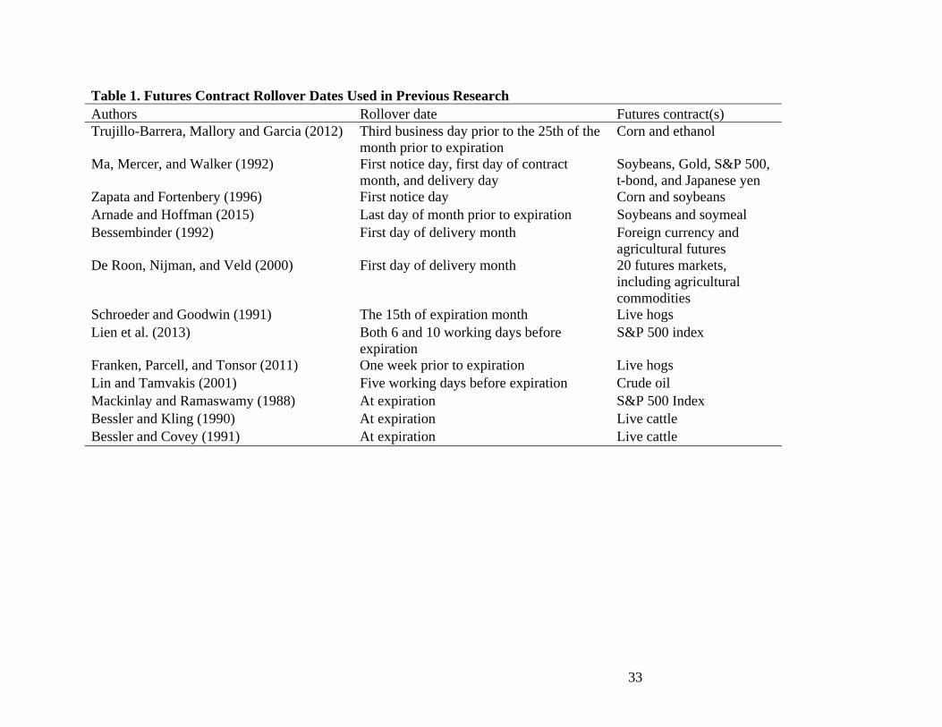
from many different contracts into a single series. Ma, Mercer, and Walker (1992) argue that

determining how and when which contracts are used is determined by the researcher can

sometimes appear quite arbitrary (Ma, Mercer, and Walker 1992). Table 1 presents the rollover

methods used by many previous studies to choose when to switch to the next available contract.

We argue that selecting the rollover point is not what is important. The primary issue with the

continuous contract approach with respect to stationarity tests is that the underlying mean is not

constant. Figure 1 shows the five corn futures contracts traded in 2015 as well as a continuous

series compiled from the nearby contract. Each of the expiring contracts clearly has a different

mean and, therefore, the nearby series is compiled of observations with five different underlying

4

means. As we will show, a series of combined contracts with differing underlying means is not

consistent with the assumptions of traditional unit root tests.

Price theory suggests that commodity spot prices should possess some level of mean

reversion (Pindyck 2001; Lautier 2005; Wang and Tomek 2007). In particular, commodity spot

prices are unlikely to sustain a level above the cost of production due to a resulting increase in

production (Dixit and Pindyck 1994). A number of other studies also suggest mean reversion in

commodity spot prices (e.g. Peterson, Ma and Ritchy 1992; Allen, Ma and Pace 1994; Walburger

and Foster 1995; Irwin, Zulauf, and Jackson 1996; Schwartz 1997; Pindyck 2001; Casassus and

Collin-Dufresne 2005; Tang 2012; Hart et al. 2015).

Contrary to the theory that commodity prices should be mean-reverting, much empirical

evidence suggests that spot prices are more likely to follow some type of unit root (i.e. random

walk) process (e.g. Ardeni 1989; Bessler and Covey 1991; Schroeder and Goodwin 1991; Beck

1994; Babula, Ruppel, and Bessler 1995; Foster, Havenner, and Walburger 1995; Zapata and

Fortenbery 1996; Barkoulas et al. 1997; Goodwin and Holt 1999; McKenzie and Holt 2000;

Harri, Nalley, and Hudson 2009; Franken, Parcell, and Tonsor 2011). Table 2 presents results

from various studies that tested commodity prices for unit roots. While this is certainly not an

exhaustive list, it shows that more often than not, tests fail to reject that commodity prices (cash

and futures) follow a unit root process. While price theory supports mean reversion in the long

run, it is hard to believe that prices are mean-reverting to a constant underlying long-run mean

even in the longest available time series. So while price theory may suggest spot prices should

revert back to the cost of production, the cost of production is not constant over time.

The changing cost of production can be seen in Figure 2 where the spot corn price in

Omaha, NE and the cost of production for a bushel of corn in Iowa are compared. While this

5

figure does not account for transportation costs, it shows that the spot price generally moves in

relation to the underlying cost of production. Perhaps more importantly, figure 2 documents the

changing cost of production for corn. Others have also documented that commodity prices do not

revert to a constant mean (e.g. Cuddington and Urzua 1987; Dempster et al. 2008). Tang (2012)

further noted that if the long-run mean is stochastic and nonstationary, mean reversion tests for a

constant mean should reject mean reversion.

Wang and Tomek (2007) argued that structural changes shift the underlying mean and

discussed the important conundrum of theory suggesting mean-reversion while many empirical

studies suggest unit root processes and stated that they found no theoretical evidence to believe

that cash commodity prices possess unit roots. Wang and Tomek (2007) suggested that not

considering structural breaks can explain why unit root tests find a series to be nonstationary.

The problem with this argument is if structural breaks are frequent enough, how does it differ

from a unit root process? Others have suggested methods to determine the frequency and

magnitude of structural breaks and how this should impact commodity price models (e.g. Zivot

and Andrews 1992; Lumsdaine and Papell 1997; Pesaran, Pettenuzzo, and Timmermann 2006;

Lee and Brorsen 2016). While these studies identify where it can be statistically shown that

structural changes occur, the underlying mean for agricultural commodities changes by at least a

small amount each crop year as production practices and costs evolve.

Whether a series is mean-reverting or possesses a unit root is important for both

theoretical and empirical models. Theoretically, the presence of unit roots suggests that short-run

departures of prices from their underlying long-run equilibriums are persistent and irreversible

which disagrees with most economic price theory (Campbell and Perron 1991). Empirically,

6

failing to account for nonstationary series in economic models can lead to spurious regression

(Granger and Newbold 1974).

Most agricultural commodities are grown on an annual basis and this can have a key

impact on when prices mean-revert as opposed to following a random walk process (though this

impact is lessened due to the storability of most commodities). Corn and soybeans in the United

States are predominantly harvested in the early fall while wheat harvest begins in late spring.

Harvest affects prices as they will either represent new crop or old crop depending on whether

the prices are prior to harvest or after harvest. Lence and Hayenga (2001) showed in a multi-year

rollover framework that it is virtually impossible to secure a high price for the next crop year by

hedging old crop futures prices. Thus, the mean reversion of spot prices may occur across crop

years while prices act as random walks within crop years (Kim and Brorsen 2012).

Futures prices in efficient markets should not wander too far from the underlying spot

value at rollover because this is where the two series must converge. If spot and futures prices

drift apart in an efficient market, arbitrage should bring them back together (Schwartz and

Szakmary 1994). Thus, we can reasonably expect that the equilibrium futures price is equal to

the expected spot price.

The changing underlying means for commodity spot prices holds a curious place in the

financial and commodity prices literature. Much attention has been paid to prices containing both

mean-reverting and random components in univariate models (i.e. to explain the behavior of one

price) of commodity prices. The seminal work by Schwartz (1997) introduced the short-term

long-term model to allow for prices to be random (i.e. follow a Brownian motion process) in the

long-run while allowing for mean reversion (i.e. Ornstein Uhlenbeck process) in the short-run.

Variations of this model have become common in the commodity price literature (e.g. Schwartz

7

and Smith 2000; Lucia and Schwartz 2002; Paschke and Prokopczuk 2010; Tang 2012; Hart et

al. 2015; etc.), though most extensively in univariate settings such as forecasting or real options

models due to the added complications of estimation (Pindyck 2001). A key drawback of these

models is that the factors are not actually observable and estimation techniques such as the

Kalman Filter (or Bayesian methods) must be applied to infer non-observable variables from

observable data (Lautier 2005). Further, these models typically assume linear mean reversion.

The linear mean reversion is an issue for agricultural crops because when prices are high mean

reversion is expected to primarily occur across crop years.

On the other hand, multivariate models using commodity prices, such as studies using the

popular Engle and Granger (1987) error correction model are performed after determining if spot

and futures price series are either mean-reverting or follow a unit root process (e.g. McKenzie

and Holt 2000; Joseph, Garcia and Peterson 2013). Error correction models are an extremely

valuable tool for estimating models that involve multiple prices that are cointegrated. However,

the first prerequisite for two series to be cointegrated is that each follows the same order unit root

process and, therefore, do not possess mean reversion.

An important motivation for this article is the apparent disconnect between how

commodity prices are treated in univariate frameworks (e.g. forecasting, options valuation, etc.)

and multivariate models of spot and futures prices (e.g. error correction models, etc.). By using

extensions from the prominent Schwartz (1997) and Schwartz and Smith (2000) models, we

argue that the current methods used to test for stationarity in multivariate analysis can be

improved. We show and suggest that panel unit root tests more adequately test the way

commodity processes actually behave. We argue that the panel unit root tests are more correctly

specified for futures prices than the current continuous contract methods used. We show

8

theoretically that the current methods for aligning commodity futures prices as continuous

contracts create a series with multiple underlying means. For cash prices, we test the hypothesis

that price series should be divided into within crop-year and across crop-year segments. Our

findings have implications for cointegration tests of cash and futures prices as a correctly

specified cointegration test is subject to the specification of cash and futures prices. Next, the

data are described and results are presented. Finally, conclusions are drawn and implications are

considered.

Conceptual Framework

To begin the discussion, consider a vector error correction model of all prices in the

economy:

1 ∆

where is a vector of prices, is a vector of the error correction terms which captures the

cointegration dynamics of spot prices with all of the other prices in the economy, is a vector

of possibly time varying intercepts, ∆ is the first difference operator, and is a stationary error

term.

This ECM includes every price. For example, there are a multitude of wheat prices as

wheat prices vary across type, location, and quality. There can be a multitude of cointegrating

vectors as well. The cointegration convergence rate in (1) is specified to vary across time.

Considerable research has found thresholds in ECM models (Goodwin and Piggot 2001; Meyer

and von Cramon-Taubadel 2004; Han, Chung, and Surathkal 2016). It is these thresholds that act

together to keep prices from going to zero or to infinity. For example, if wheat prices fall enough

9

cattle feeders begin feeding wheat so wheat and corn prices become cointegrated. Further, many

parameters change over time due to changes in technology, government policies and tastes and

preferences. Thus, while such a model may describe the actual economy as a whole, a simplified

model is needed to make it empirically tractable.

One such univariate model is the Ornstein-Uhlenbeck (OU) model and assumes that price

follows a stochastic mean-reverting process. The OU process is shown as the solution of a

stochastic differential equation as

2

where is the commodity spot price, is the long-run mean spot price, is the mean reversion

speed, and are increments to a standard Brownian motion process. The OU process is the

continuous time version of a stationary first order autoregressive process (AR(1)). The model

assumes that the long-run mean is a constant.

The OU model in equation (2) can be extended by allowing the long-run equilibrium to

possess a unit root and differing rates of adjustment for the mean reverting and unit root

processes. These extensions lead to one of the most prominent financial models as derived by

Schwartz and Smith (2000) is built around this assumption. We use their two factor model to

express the dynamics of commodity prices. This is not a novel concept. Autoregressive

integrated moving average ARIMA forecasting models and other literature have long suggested

both mean reversion and random components. This model for a commodity spot price allows for

mean reversion and uncertainty in the equilibrium level to which prices revert and is written as

3

10

where denotes the log of the spot price (to ensure positive prices) of a commodity in year

and is decomposed into two stochastic factors to represent short-term deviations ( as well as

the stochastic long-run equilibrium ( . Note that these two factors are not actually observable

for most commodity prices. These factors must be inferred from available data such as long-

maturity futures contracts to provide information about the long-run equilibrium and differences

between long-term and short-term futures prices to provide information about short-run

deviations (Lautier 2005).

Seasonality is also well-documented in commodity price series. Sørensen (2002) used a

deterministic seasonal component to account for pronounced seasonal patterns in the prices of

soybeans, corn and wheat. Jin et al. (2012) and Hart et al. (2015) used similar approaches to

correct for seasonality in commodity prices while Paschke and Prokopczuk (2009) found

seasonal effects in natural gas, heating oil, and gasoline. Others have also considered seasonality

as playing an important role in specifying commodity prices (Manoliu and Tompaidis 2002;

Lucia and Schwartz 2002; Brooks, Prokopczuk, and Wu 2013). Todorova (2004) and Mirantes et

al. (2012) model seasonality as a stochastic factor. Kim and Brorsen (2012) used a seasonal

mean reversion model to estimate when producers should sell stored grain. They found that,

unless prices are extremely low, it is optimal for producers to sell stored grain before the mean

reversion begins which they found to be between 38 weeks and 42 weeks after harvest for corn,

soybeans, and wheat. Since our focus is on agricultural commodities, we also include seasonality

in the spot price (e.g. Sørensen 2002, Schwartz and Smith 2000; Manoliu and Tompaidis 2002;

and Todorova 2004). Thus, we amend equation (3) to become

4

11

where is a seasonality term similar to Sørensen (2002) used to capture the seasonality

effects inherent to most agricultural production practices. Similar to Schwartz and Smith (2000),

the short-term (mean reversion) state variable follows an Ornstein-Uhlenbeck process with

mean reversion parameter and volatility parameter , and the stochastic long-term state

variable follows a Brownian motion process with drift rate and diffusion rate as shown in

5

6

where and are standard Weiner processes and are assumed to have a constant

correlation coefficient . As in Tang (2012), the factor can be thought of as accounting for

permanent shocks while is the mean reversion factor.

Note that the Schwarz-type models are approximations to the true stochastic process in

(1). For a storable commodity, arbitrage should constrain expected price rises to not exceed the

rate of storage cost and can occur gradually as assumed in the model. But, price decreases for a

seasonal commodity such as corn should occur across crop years and are unconstrained in size.

Further, cointegration thresholds should prevent prices from going as high or as low as is

allowed by the Brownian motion assumption. In addition, as is widely recognized, there can be

structural change in parameters. We continue by using equation (4), but acknowledge that it is an

approximation.

Futures Prices

We are next interested in deriving futures prices using the spot price. Forward prices have

been shown to be essentially equal to the expected future spot price at maturity under the risk-

12

neutral framework assumption that interest rates are constant (Cox, Ingersoll, and Ross 1981;

Duffie and Stanton 1992). Thus, we must adjust the spot price equations for risk neutrality in

order to derive the model for futures prices. Following the risk adjustment procedure used by

Schwartz and Smith (2000) and Lucia and Schwartz (2002), we develop the risk neutral model

for spot price by introducing market price of risk parameters and into the risk neutral

stochastic processes of and in equations (3) and (4), respectively, to specify assumed

constant reductions in the drifts of each process. The processes then take the form

7

8

where the risk-neutral mean reversion process now reverts to / instead of zero and the

drift in the Brownian motion process is now . Under the risk neutral framework of

Lucia and Schwartz (2002), the futures price is the expected cash price at maturity:

9 , 1

where , denotes the futures price at time zero with time until maturity, / and

.

Whereas spot prices are generally reported in a true continuous fashion, time series data

for futures prices comes from multiple futures contracts. Since theory and arbitrage demand that

spot prices and futures prices converge at maturity, the possibly gradual mean reversion in cash

prices is expected to be reflected in discrete jumps in futures prices at rollover. We can show the

behavior of futures price spreads at maturity using the model above. Using equations (9) and (4),

the expected change at rollover can be calculated. To solve for this, we look at the calendar

spread at the time of rollover:

13

10 , , 1 1

where H denotes the time to the next contract maturity. The only pieces left are seasonality

, the mean reversion expected over the interval, and the latent factors and . Thus,

across contracts (at rollover), we can expect that futures prices will be mean reverting and the

rollover point should be treated differently from the rest of the series.

Differencing a series of continuous contracts is complicated by the switching of

contracts. Equation (9) shows that every futures contract has a different expected value and so

combining multiple contract months results in differing means as contract maturity month

changes. Differences taken between the last observation used of a contract and the first

observation used of the next contract include the terms in (10), which can lead to outliers at the

point where contracts are spliced together. Including a single dummy variable as in Franken,

Parcell, and Tonsor (2011) only removes the mean of the spread terms in (10) and so the outliers

remain. Including a different dummy variable for every rollover still leaves the outliers in the

lagged values. Most past research has used differences taken before splicing, which eliminates

the problem with outliers. However, splicing still combines differences from contracts with

differing expected values.

Tests for Stationarity

The Schwartz models suggest that commodity prices are comprised of both mean

reverting and unit root processes. However, empirical estimation of these models is complicated

by latent factors whose distribution must be inferred from observable data. The difficulty in

14

estimating the Schwartz model is a key reason that it is almost standard practice to instead

assume a one-factor model where prices are either mean-reverting or follow a unit root.

One of the first tests performed in much commodity price analysis research is to test for

a unit root. When working with both cash and futures data, generally, unit root tests are

performed for each series and these results are used to determine if data transformations and

cointegration tests are needed. Futures price series are often considered to have a unit root as

they are thought to follow a random walk. The jury is less settled on unit roots in spot

commodity prices as arguments such as Wang and Tomek (2007) and some empirical works do

not support spot prices possessing unit roots. However, plenty of research has empirically found

unit roots for spot price series.

The common practice of determining stationarity in commodity price series pits mean

reversion and unit roots against each other and claims the winner to be the manner in which the

series behaves. Thus, the reason so many empirical studies determine that prices must follow a

unit root is because the random component outweighs the mean reversion component by enough

to satisfy (or fail to reject) a statistical test such as Dickey and Fuller (1981) or Phillips and

Perron (1988). It is certainly possible that the random component will dominate the mean

reversion component in most available price series. Pindyck (1999) argued that even with series

spanning more than a century, unit root tests are likely to be inconclusive due to the slow nature

of mean reversion. He also suggested that the trend to which prices are reverting fluctuates over

time. The storable nature of commodities also suggests that prices might mean-revert downward

faster than they do upward since some participants may be in a position to wait-out low prices.

15

Perhaps the most common unit root test is the Dickey Fuller (DF) Test and its augmented

version (ADF) (Dickey and Fuller 1981). We now consider the effects of applying the DF test to

data generated from a Schwarz-type process. Consider a DF type regression

11

where denotes a price series and is the mean reversion parameter. Rejecting the null

hypothesis of the DF test (and most univariate unit root tests) implies that the series mean-reverts

in the long-run. If the intercept in (11) is zero then the convergence is to a constant price level. If

the intercept is not zero, then convergence is to a linear trend. Failure to reject the null

hypothesis of nonstationarity implies there is not enough statistical evidence to conclude against

the process possessing a unit root. As specified by the conceptual model, an important weakness

of the ADF test is that the underlying mean is changing. With futures, the mean differs with

every change in contract maturity. With cash prices, the mean differs due to changes in the cost

of production and the issue is how close these changes are to the linear trend assumed with a DF

test. We now discuss the econometric problems from using the DF tests with futures and spot

prices.

Unit Root Tests for Futures Prices

Using (13), the standard DF test for a commodity futures price series can be written as

12

where denotes the mean reversion coefficient. The general practice is to test the null

hypothesis of 1 which would imply the series possesses a unit root. However, also of

interest is the underlying assumption of the alternative hypothesis. By adding and subtracting the

16

constant underlying mean from in (12), it can be shown that the mean reversion

coefficient is estimating the rate of convergence to as in

13 .

Therefore, alternative hypothesis of 1 is that the futures price reverts to a constant mean.

However, as was shown in (9) and (10), the expected values differ across futures contracts. Thus,

the test shown in (13) would only apply to observations from a single contract month.

Performing this test on a continuous contracts series would fail to account for the different of

each contract. Failing to account for a change in the underlying mean implies that the DF test is

biased towards a false acceptance of a unit root (Wang and Tomek 2007). Perron (1990) showed

that approaches one as the magnitude of even a single change in the mean increases.

Much research has focused on how to accommodate a changing level of the underlying

mean in unit root tests with respect to structural breaks. Perron (1989, 1990) and Perron and

Vogelsang (1992) extended the ADF test to allow for structural breaks. Wang and Tomek (2007)

modeled structural changes in spot milk prices and found that once these breaks were considered,

some unit root tests switched from nonstationary to stationary. Arnade and Hoffman (2015)

followed an approach similar to Zivot and Andrews (1992) to test for structural breaks in

soybeans and soybean meal spot and futures prices. They identified three sub-periods with

significantly different estimated coefficients on the lagged price of each unit root equation.

Joseph, Garcia, and Peterson (2013) also used the Zivot and Andrews (1992) test and found a

break in the mean level and trend for boxed beef prices around the 2008 financial crash. Lee and

Brorsen (2016) specified a general model that included both mean-reverting and unit root

processes as special cases and found that most shocks are permanent breaks for Oklahoma hard

winter wheat, Illinois corn, and Illinois soybean basis which favors a unit root model.

17

The literature on structural breaks is similar to our scenario of a changing mean across

futures contracts. However, most of the structural break methodology is suited for series with

unknown periods of changing means. If breaks are infrequent and discrete, then the Zivot and

Andrews (1992) approach should capture the necessary dynamics. In the case of commodity

futures prices, we know the underlying mean changes for each futures contract. Therefore, each

contract should be treated as its own cross-section. We suggest using a single contract for each

crop year and we can amend (15) to allow for a different mean for each crop year’s contract

14

where denotes the underlying mean for each crop year (contract) . As a result, the univariate

DF test is no longer applicable to the panel of futures contracts in (14). However, panel unit root

tests can be used to get a joint test of the null hypothesis of a unit root.

Unit Root Tests for Spot Prices

The underlying mean of the spot price is expected to be related to the long-run marginal cost of

production. If this mean is constant or follows a time trend, then the DF test in (12) would be

correctly specified. However, if the cost of production changes stochastically each crop year as

we hypothesize, then an adjustment is needed to allow for a different mean each year. Within the

Schwartz model, this would imply the assumption that long-run equilibrium changes each

year. This changing mean can be accounted for by specifying spot price process in (4) as

15

where represents crop year. We must also consider the impact of our hypothesis that mean

reversion occurs across crop years while prices follow a unit root within a crop year. This

18

requires the assumption that the mean reversion level in (5) is a different level between crop

years relative to within crop years. Specifically, we assume that 0 within a crop year and

0 between crop years as the new crop approaches. We can account for this assumption by

creating separate panels for the “within crop year” period and “between crop year” period.

Panel Unit Root Tests

We use panel unit root tests as they allow the underlying mean to vary across panels (e.g.

crop years) as is specified in (14). We specify the following panel tests for futures prices, though

they also apply for our specification of spot prices. However, spot prices are divided into

separate panels for “within crop year” period and “between crop year” periods.

We begin with the popular Levin, Lin, and Chu (LLC) (2002) panel unit root test

16 ∆ ∆

where 1,… , denotes the number of panels and represents the number of observations in

each panel, represents any trend effects within each panel, is the speed of adjustment (mean

reversion parameter), and is the lag length. For this test, the null hypothesis is that 0 for all

panels ( ) and the alternative is that 0 for all panels. Thus, while the underlying means can

be different across panels, the level of mean reversion is assumed to be constant across all panels

which is similar to that of the DF and ADF tests.

Im, Pesaran, and Shin (2003) which we will denote as IPS, used a similar framework to

LLC (2002), but relaxed the assumption of homogeneous rate of mean reversion for all panels.

19

While the rate of mean reversion is assumed to be constant for each panel in our model1, we

include the IPS (2003) test to account for a possible change in the rate of mean reversion across

crop years. Differing mean reversion rates would imply that prices mean-revert faster in some

years than in others. The IPS (2003) panel unit root test is specified as

17 ∆ ∆

where the speed of adjustment is now allowed to be heterogeneous across panels and all other

components are as defined in (16). The unit root test within each panel is based on the ADF

statistics and results are averaged across panels to provide a single test statistic for the data as

shown by

18 ̅1

where are the statistics for each panel . The null hypothesis for the IPS (2003) test is that all

0 compared to the alternative hypothesis that at least one of the panels is stationary.

Cointegration

The ideas on cointegration are not as fully developed as the rest of the paper, but we

discuss cointegration anyway. A prerequisite for two series to be cointegrated is that they both

follow a unit root process of the same order. If this condition holds, and there exists a linear

combination of the two series that is stationary, then the variables can be defined as cointegrated

1 Note the mean reversion level is hypothesized to be different for between crop year and within crop year segments for cash prices. However, we split cash prices in to separate panels for these two periods. Therefore each panel is assumed to have a constant mean reversion level.

20

(Engle and Granger 1987). By specifying the ECM equation from (1) with futures price as the

dependent variable, we can use the solutions for spot (equation 4) and futures (equation 9) prices

to show the cointegrating relationship between futures and spot prices to be

19 ∆

where includes the latent factors 1 from (9) and captures any expectation

differences between the futures price and the expected spot price. The error correction term

is the linear combination of and and is represented by which, by

substitution, can be specified as

20

where the terms are the unit root terms for futures and spot prices and are offset for any single

time period , is the difference in seasonality, and is the difference

between the mean reversion terms. A correctly specified cointegration test would account for the

differences in mean reversion and seasonality. Alternatively, a plausible assumption can be made

for each difference to be negligible at any single time period. Spot and futures prices are

theoretically cointegrated under the assumptions of the Schwartz model. Empirical estimation of

this cointegration model would require the use of latent factors that must be inferred from

observable data. Though it is beyond the scope of this paper, it might be possible for these to be

inferred from futures prices as in Hart et al. (2015). Panel unit root tests can help model

differences in mean reversion when 0. Alternatively, for the case of 0, univariate unit

root tests are appropriate.

By definition, cash and futures prices are cointegrated at maturity. To conduct a

cointegration test using daily prices, the other factors such as cash price seasonality need to be

21

considered in the model. Most past empirical research has used daily prices and has not included

variables to reflect cash price seasonality or cash market mean reversion. When empirical

research has found cointegration in the past, it may mean that the seasonality and mean reversion

factors are relatively small.

Data

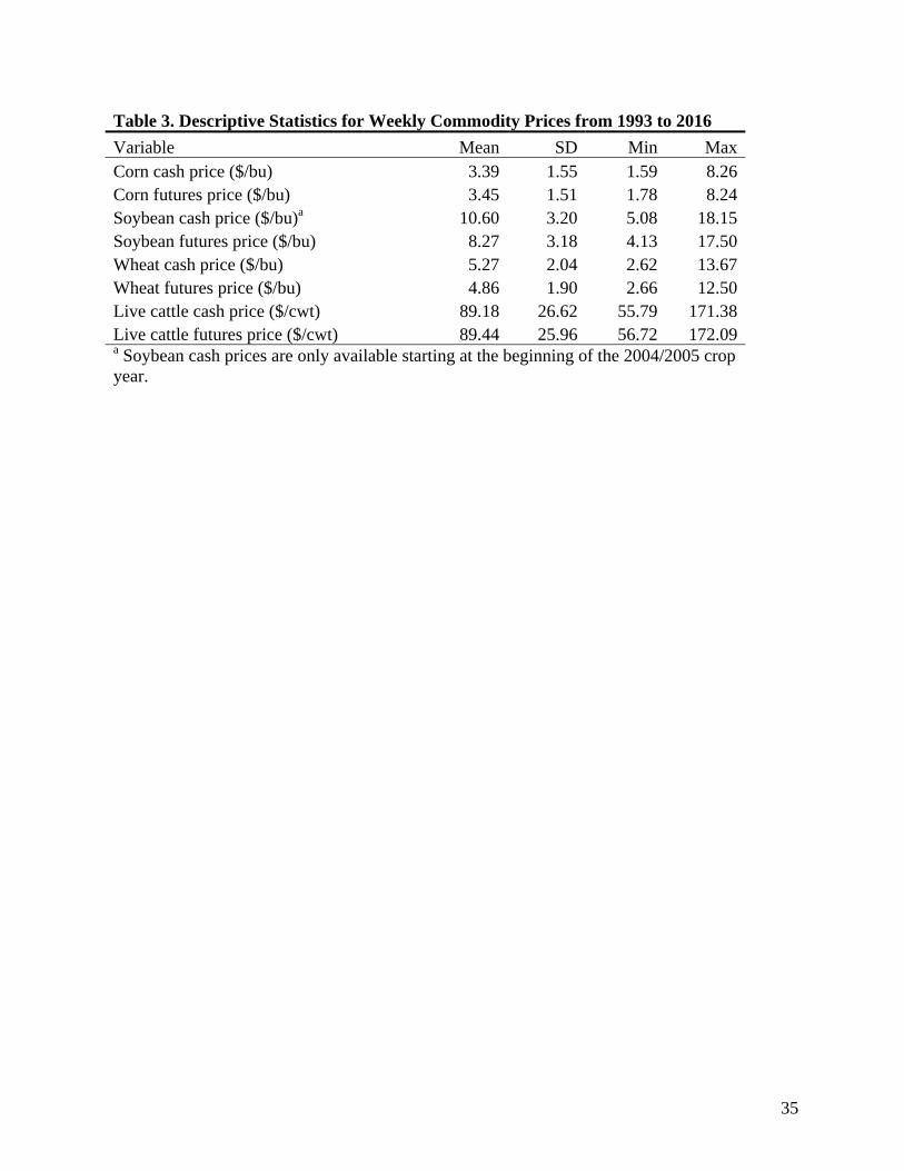
We perform the unit root tests on weekly cash and futures prices for corn, soybeans,

wheat, and live cattle compiled by the Livestock Marketing Information Center (LMIC). All

grain prices except soybean cash prices span from the beginning of the 1993/1994 crop year

through the 2015/2016 crop year. Soybean cash prices were only available in this data set from

the beginning of the 2004/2005 crop year through the end of the 2015/2016 crop year. The crop

year for corn and soybeans begins on October 1st each year as suggested by Smith (2005). Wheat

crop years start on June 1st each year. Since live cattle are produced throughout the year, calendar

year panels are used. Summary statistics are provided in table 3. Corn cash prices are as reported

in Chicago, IL and wheat cash prices are for hard red winter wheat #1 in Kansas City, MO and

both are from the National Weekly Feedstuff Wholesale Prices reports (USDA, AMS 2016c).

Soybean cash prices are as reported in central Illinois and are from the Soybean Prices

Compared with Value of Oil and Meal reports (USDA, AMS 2016b). All grain prices are quoted

in dollars per bushel ($/bu). Live cattle cash prices are in dollars per hundred pounds ($/cwt) and

are reported by the Five Area Weekly Weighted Average Direct Slaughter Cattle reports (USDA,

AMS 2016a).

Grain futures prices are weekly futures prices in $/bu for Wednesday of each week. If

Wednesday falls on a holiday, the Thursday price is used for that week. Live cattle futures prices

22

are reported in $/cwt. We use a single contract for each crop year in order to avoid a combination

of contracts with differing means This panel approach avoids the combination of multiple

contracts with differing underlying means as discussed in (14). For corn and soybeans, we use

the May contract prices and thus our panel for each crop year spans from the first week in

October through the second week in April. We avoid observations near maturity as is common in

the commodity price literature as shown in table 2. For wheat, we use the March contract prices

for each crop year and each panel spans from the first week in June through the last week in

January. Live cattle futures prices are for the December contract and each panel is from the first

week in January through the second week in November.

The LLC (2002) test requires balanced panels and thus missing observations and varying

numbers of weeks in each crop year create a problem for this test. The only missing observations

occur in cash prices where two weekly prices were missing for corn and wheat and nine weekly

prices were missing for soybeans. To fill these missing observations, we add the change in the

futures price for the corresponding date and commodity to the most recent cash price. To account

for a varying number of weekly observations per year, observations occurring on the first or last

day of a crop year are omitted (i.e. September 30th or October 1st for corn and soybean prices).

This results in each crop year possessing the balanced panels needed for the LLC (2002) test.

Empirical Results

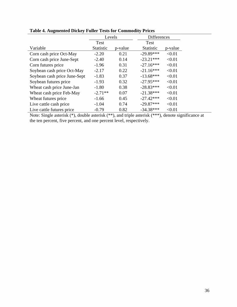
We begin by testing each series for stationarity using the traditional ADF test. This test

assumes a constant underlying mean. Table 4 reports the results of the ADF test for each

commodity price series in levels and in differences. As shown, the ADF test fails to reject the

null hypothesis of a unit root for each price series in levels except for wheat futures prices and

23

wheat cash prices for February through May. The finding of mean reversion in wheat futures is

surprising. The finding of mean reversion for cash prices is to be expected, especially in the

between crop year span. All other variables are nonstationary according to the ADF in levels.

After taking the first differences, the ADF tests reject the null hypothesis and appear stationary.

Thus, we would conclude that each series, besides wheat, is 1 from these results alone as is

done in most of the studies listed in table 1 though this is certainly not an exhaustive list.

We next consider the LLC (2002) panel unit root test which assumes a constant rate of

mean reversion across panels. Thus, for each commodity price series, the number of panels

corresponds with the number of years available and the number of observations per year

corresponds with the number of weeks in each year. Table 5 reports the results from this test. As

shown, both series of corn and wheat cash prices are found to be mean-reverting in at least one

panel. Likewise, wheat futures prices are found to be mean-reverting in at least one panel, an

unexpected result. The LLC (2002) test fails to reject the null hypothesis of unit roots in all

panels for the remaining variables.

Further exploration of wheat futures prices finds that upon deletion of observations after

2006, the null hypothesis of a unit root cannot be rejected. Thus, the finding of mean reversion in

wheat futures prices is found only after 2006. This implies that the finding of mean reversion is

driven by recent years when wheat prices have experienced dramatic changes. One possible

explanation is the occurrence of a bubble in commodity prices around 2007-2008. A common

concern is that increased buying pressure from financial index investors led to bubbles in

commodity futures prices (e.g. Masters, 2008 2009). Other financial activity such as managed

funds are also considered to have had an impact (Waggoner 2008). Empirical results are mixed

on whether financial activity led to a bubble in wheat prices. Etienne, Irwin, and Garcia (2015)

24

provide an excellent discussion on the possibility of a bubble in wheat futures prices and found

that any impact should be negligible. Alternatively, Gutierrez (2013) found support for a bubble

in wheat prices, though he was unable to conclude that the bubble was caused specifically by

financial activity. Our results are unable to offer specific insights on a bubble in wheat futures.

However, we do find different wheat futures price behavior after 2006.

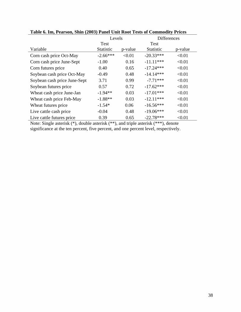
Next, we use the IPS (2003) panel unit root test to test each series for stationarity. This

test allows for varying speed of adjustment as the panel is constructed across years to account for

changing dynamics across crop years. As shown in table 6, the IPS (2003) panel unit root test

results are similar to the LLC (2002) results. The IPS (2003) test fails to reject the null

hypothesis of a unit root process in levels for all commodities except corn and wheat. The

presence of a unit root process is rejected for corn cash prices from October to May at the one

percent level and for corn futures prices at the ten percent level. Wheat cash prices are found to

be stationary at the five percent level and wheat futures prices at the one percent level. Similar to

the ADF test, after taking the first difference, every price series appears stationary.

Our hypothesis of mean reversion between crop years and a random walk within crop

years is generally not supported. For each of the crops considered the LLC (2002) test results in a

conclusion of mean reversion for both periods for corn and wheat cash prices and a conclusion of

a unit root for both periods of soybean cash prices. Our results differ from traditionally used unit

root tests shown in table 2 as we find mean reversion in corn and wheat cash prices. In particular,

Wang and Tomek (2007) found that accounting for structural changes in the underlying mean

can result in finding cash prices to be mean-reverting. Our results extend on this work by

allowing the underlying means to change each crop year.

25

Conclusions

Determining whether a series is mean-reverting or follows a unit root process is an

integral part of time series analysis as it is often one of the first things tested. There seems to be a

growing divide between how univariate analysis accounts for mean reversion as compared to

multivariate analysis. In particular, the Schwartz-type (year) two factor models allow for some

level of both mean reversion and unit roots whereas the popular error correction models require

the researcher to determine if prices are either mean-reverting or follow a unit root process. Our

application of panel unit root tests incorporates a key assumption from the Schwartz-type models

(i.e. a changing underlying mean, though only across crop years). Thus, while we still ultimately

find a series to be either mean-reverting or nonstationary, the results are from a test that allows

for the changing underlying means.

We show that continuous contracts do not account for differing underlying means for

each contract and for the mean reversion that occurs at rollover. Panel unit root tests are used by

treating each crop year as a panel. The traditional unit root tests are unable to account for a

possible shift in the underlying mean across crop years. It should not be expected that using

panel unit root tests will drastically change results of previous studies. However, it is likely that

results might be less sporadic due to a more uniform specification of the changing underlying

mean.

Cash prices are difficult as none of the currently available models captures their likely

stochastic process. The hypothesis that prices within a crop year and across a crop year should be

treated as having differing mean reversion behavior is not well supported by our results.

However, aligning cash prices as a single continuous series does not account for deviations from

a linear trend for cost of production over time.

26

While the mean reversion in cash prices is easier to understand, the finding of mean

reversion in wheat futures prices contrasts with the theory that futures prices should follow a unit

root process. Further exploration using the LLC (2002) test found that this mean reversion was

driven by price behavior in recent years. One possible explanation is trading by managed funds

in recent years may have accentuated price swings.

The implications of our findings are important as they can influence modelling

techniques. While the panel unit root tests are more appropriate for futures prices, the correct

approach for cash prices is less clear-cut. Since cointegration tests rely on each price series,

differing alignments of prices create difficulties in correctly specifying cointegration tests.

27

References

Allen, M. T., C. K. Ma, and R. D. Pace. 1994. “Over-Reactions in US Agricultural Commodity Prices.” Journal of Agricultural Economics 45 (2): 240-251.

Ardeni, P. G. 1989. “Does the Law of One Price Really Hold for Commodity Prices?” American Journal of Agricultural Economics 71 (3): 661-669.

Arnade, C., and L. Hoffman. 2015. “The Impact of Price Variability on Cash/Futures Market Relationships: Implications for Market Efficiency and Price Discovery” Journal of Agricultural and Applied Economics 47 (4): 539-559.

Babula, R. A., F. J. Ruppel, and D. A. Bessler. 1995. “US Corn Exports: The Role of the Exchange Rate.” Agricultural Economics 13 (2): 75-88.

Barkoulas, J., W. C. Labys, and J. Onochie. 1997. “Fractional Dynamics in International Commodity Prices.” Journal of Futures Markets 17 (2): 161-189.

Beck, S. E. 1994. Cointegration and Market Efficiency in Commodities Futures Markets.” Applied Economics 26: 249-257.

Bessembinder, H. 1992. “Systematic Risk, Hedging Pressure, and Risk Premiums in Futures Markets.” Review of Financial Studies 5 (4): 637-667.

Bessler, D. A., and T. Covey. 1991. “Cointegration: Some Results on U.S. Cattle Prices.” The Journal of Futures Markets (11): 461–474.

Brooks, C., M. Prokopczuk, and Y. Wu. 2013. “Commodity Futures Prices: More Evidence on Forecast Power, Risk Premia and the Theory of Storage.” Quarterly Review of Economic Finance 53 (1): 73-85.

Campbell, J., and P. Perron. 1991. “Pitfalls and Opportunities: What Macroeconomists Should Know about Unit Roots.” Macroeconomics Conference, National Bureau of Economic Research, Cambridge, MA, February.

Casassus, J., and P. Collin-Dufresne. 2005. “Stochastic Convenience Yield Implied from Commodity Futures and Interest Rates.” Journal of Finance 60 (5): 2283–2331.

Chen, S. L., J. D. Jackson, H. Kim, and P. Resiandini. 2014. “What Drives Commodity Prices?” American Journal of Agricultural Economics 96 (5): 1455-1468.

Cox, J. C., J. E. Ingersoll, and S. A. Ross. 1981. “The Relation between Forward Prices and Futures Prices.” Journal of Financial Economics 9 (4): 321-346.

Cuddington, J., and M. Urzu. 1987. “Trends and Cycles in Primary Commodity Prices.” Economics Department, Georgetown University, Washington, DC. Processed Paper.

28

De Roon, F. A., T. E. Nijman, and C. Veld. 2000. “Hedging Pressure Effects in Futures Markets.” The Journal of Finance 55 (3): 1437-1456.

Dempster, M., E. Medova, and K. Tang. 2008. “Pricing and Hedging Long-Term Spread Options.” Journal of Banking Finance 32: 2530–2540.

Dickey, D. A., and W. A. Fuller. 1981. “Likelihood Ratio Statistics for Autoregressive Time Series with a Unit Root.” Econometrica 49: 1057-1072.

Dixit, A. K., and R. S. Pindyck. 1994. “Investment Under Uncertainty.” Princeton University Press, Princeton, NJ.

Duffie, D., and R. Stanton. 1992. “Pricing Continuously Resettled Contingent Claims.” Journal of Economic Dynamics and Control 16 (3): 561-573.

Engle, R., and C. Granger. 1987. “Co-Integration and Error Correction: Representation, Estimation, and Testing.” Econometrica 55: 251–276.

Etienne, X. L. S. H. Irwin, and P. Garcia. 2015."$25 Spring Wheat was a Bubble, Right?" Agricultural Finance Review 75 (1): 114 – 132.

Foster, K. A., A. M. Havenner, and A. M. Walburger. 1995. “System Theoretic Time-Series Forecasts of Weekly Live Cattle Prices.” American Journal of Agricultural Economics 77 (4): 1012-1023.

Franken, J. R., J. L. Parcell, and G. T. Tonsor. 2011. “Impact of Mandatory Price Reporting on Hog Market Integration.” Journal of Agricultural and Applied Economics 43 (02): 229-241.

Goodwin, B. K., and M. T. Holt. 1999. “Price Transmission and Asymmetric Adjustment in the US Beef Sector.” American Journal of Agricultural Economics 81 (3): 630-637.

Goodwin, B. K., and N. E. Piggott. 2001. "Spatial Market Integration in the Presence of Threshold Effects." American Journal of Agricultural Economics 83 (2): 302-317.

Granger, C. W. J., and P. Newbold. 1974. "Spurious Regressions in Econometrics." Journal of Econometrics 2 (2): 111-120.

Gutierrez, L. 2013. “Speculative Bubbles in Agricultural Commodity Markets.” European Review of Agricultural Economics 40 (2): 217-238.

Han, S., C. Chung, and P. Surathkal. 2016. “Impacts of Increased Corn Ethanol Production on Price Asymmetry and Market Linkages in Fed Cattle Markets.” Agribusiness 1-25.

Harri, A., L. Nalley, and D. Hudson. 2009. “The Relationship between Oil, Exchange Rates, and Commodity Prices.” Journal of Agricultural and Applied Economics 41 (2): 501-510.

29

Hart, C. E., S. H. Lence, D. J. Hayes, and N. Jin. 2016. “Price Mean Reversion, Seasonality, and Options Markets.” American Journal of Agricultural Economics 98 (3): 707-725.

Im, K., H. Pesaran, and K. Shin. 2003. “Testing for Unit Roots in Heterogeneous Panels.” Journal of Econometrics 115 (1): 53-74.

Irwin, S. H., C. R. Zulauf, and T. E. Jackson. 1996. “Monte Carlo Analysis of Mean Reversion in Commodity Futures Prices.” American Journal of Agricultural Economics 78 (2): 387-399.

Jin, N., S. Lence, C. Hart, and D. Hayes. 2012. “The Long-Term Structure of Commodity Futures.” American Journal of Agricultural Economics 94 (3): 718-735.

Joseph, K., P. Garcia, and P. E. Peterson. 2013. “Price Discovery in the U.S. Fed Cattle Market.” In Proceedings of the NCCC-134 Conference on Applied Commodity Price Analysis, Forecasting, and Market Risk Management, St. Louis, MO.

Kim, H. S., and B. W. Brorsen. 2012. "Can Real Option Value Explain Apparent Storage at a Loss?" Applied Economics 44 (16): 2081-2090.

Lautier, D. 2005. “Term Structure Models of Commodity Prices: A Review.” The Journal of Alternative Investments 8 (1): 42.

Lee, Y., and B. W. Brorsen. 2016. “Permanent Shocks and Forecasting with Moving Averages.” Applied Economics 1-13.

Lence, S. H., and M. L. Hayenga. 2001. "On the Pitfalls of Multi-year Rollover Hedges: The Case of Hedge-to-Arrive Contracts." American Journal of Agricultural Economics 83 (1): 107-119.

Levin, A., C. F. Lin, and C. S. J. Chu. 2002. “Unit Root Tests in Panel Data: Asymptotic and Finite-Sample Properties.” Journal of Econometrics 108 (1): 1-24.

Lien, D., G. Lim, L. Yang, and C. Zhou. 2013. “Dynamic Dependence between Liquidity and the S&P 500 Index Futures‐Cash Basis.” Journal of Futures Markets 33 (4): 327-342.

Lin, S. X., and M. N. Tamvakis. 2001. “Spillover Effects in Energy Futures Markets.” Energy Economics 23 (1): 43-56.

Lucia, J. J., and E. S. Schwartz. 2002. “Electricity Prices and Power Derivatives: Evidence from the Nordic Power Exchange.” Review of Derivatives Research 5 (1): 5-50.

Lumsdaine, R. L., and D. H. Papell. 1997. “Multiple Trend Breaks and the Unit-Root Hypothesis.” Review of Economics and Statistics 79 (2): 212-218.

Ma, C. K., J. M. Mercer, and M. A. Walker. 1992. “Rolling Over Futures Contracts: A Note.” Journal of Futures Markets 12 (2): 203-217.

30

MacKinlay, A. C., and K. Ramaswamy. 1988. “Index-Futures Arbitrage and the Behavior of Stock Index Futures Prices.” Review of Financial Studies 1 (2): 137-158.

Manoliu, M., and S. Tompaidis. 2002. “Energy Futures Prices: Term Structure Models with Kalman Filter Estimation.” Applied Mathematical Finance 9 (1): 21-43.

Masters, M.W. 2008. Testimony before the Committee on Homeland Security and Governmental Affairs, Unites States Senate. May 2008.

Masters, M.W. 2009. “Testimony before the Commodities Futures Trading Commission. August 5th, 2009.

McKenzie, A. M., and M. T. Holt. 2000. “Market Efficiency in Agricultural Futures Markets.” Applied Economics 34: 1519-1532.

Meyer, J., and S. von Cramon‐Taubadel. 2004. "Asymmetric Price Transmission: A Survey." Journal of Agricultural Economics 55 (3) : 581-611.

Paschke, R., and M. Prokopczuk. 2009. “Integrating Multiple Commodities in a Model of Stochastic Price Dynamics.” Journal of Energy Markets 2 (3): 47-82.

Paschke, R., and M. Prokopczuk. 2010. “Commodity Derivatives Valuation with Autoregressive and Moving Average Components in the Price Dynamics.” Journal of Banking and Finance 34 (11): 2742-2752.

Perron, P. 1989. “The Great Crash, the Oil-Price Shock, and Unit-Root Hypothesis.” Econometrica 57 (6): 1361-1401.

Perron, P. 1990. “Testing for a Unit Root in a Time Series with a Changing Mean.” Journal of Business & Economic Statistics 8 (2): 153-162.

Perron, P, and T. J. Vogelsang. 1992. "Testing for a Unit Root in a Time Series with a Changing Mean: Corrections and Extensions." Journal of Business & Economic Statistics 10 (4): 467-470.

Pesaran, M. H., D. Pettenuzzo, and A. Timmermann. 2006. “Forecasting Time Series Subject to Multiple Structural Breaks.” The Review of Economic Studies 73 (4): 1057-1084.

Peterson, R. L., C. K. Ma, and R. J. Ritchey. 1992. “Dependence in Commodity Prices.” Journal of Futures Markets 12 (4): 429-446.

Phillips, P. C., and P. Perron. 1988. “Testing for a Unit Root in Time Series Regression.” Biometrika 75 (2): 335-346.

Pindyck, R. S. 2001. “The Dynamics of Commodity Spot and Futures Markets: A Primer.” The Energy Journal 22: 1-29.

31

Saghaian, S. H. 2010. “The Impact of the Oil Sector on Commodity Prices: Correlation or Causation?” Journal of Agricultural and Applied Economics 42 (3): 477-485.

Schroeder, T. C., and B. K. Goodwin. 1991. “Price Discovery and Cointegration for Live Hogs.” The Journal of Futures Markets 11 (6): 685-696.

Schwartz, E. 1997. “The Stochastic Behavior of Commodity Prices: Implications for Valuation and Hedging.” Journal of Finance 52 (3): 923–973.

Schwartz, E, and J. Smith. 2000. “Short-Term Variations and Long-Term Dynamics in Commodity Prices.” Management Science 46: 893–911.

Schwarz, T. V., and A. C. Szakmary. 1994. “Price Discovery in Petroleum Markets: Arbitrage, Cointegration, and the Time Interval of Analysis.” Journal of Futures Markets 14 (2): 147-167.

Smith, A. 2005. "Partially Overlapping Time Series: A New Model for Volatility Dynamics in Commodity Futures." Journal of Applied Econometrics 20 (3): 405-422.

Sørensen, C. 2002. “Modeling Seasonality in Agricultural Commodity Futures.” Journal of Futures Markets 22 (5): 393–426.

Tang, K. 2012. “Time-Varying Long-Run Mean of Commodity Prices and the Modeling of Futures Term Structures.” Quantitative Finance 12 (5): 781-790.

Todorova, M. I. 2004. “Modeling Energy Commodity Futures: Is Seasonality Part of It?” The Journal of Alternative Investments 7 (2): 10-32.

Tomek, W.G. 1997. “Commodity Futures Prices as Forecasts.” Review of Agricultural Economics 19 (1): 23-44.

Trujillo-Barrera, A., M. Mallory, and P. Garcia. 2012. “Volatility Spillovers in US Crude Oil, Ethanol, and Corn Futures Markets.” Journal of Agricultural and Resource Economics 37 (2): 247-262.

U.S. Department of Agriculture, Agricultural Marketing Service (USDA, AMS). 2016a. Five Area Weekly Weighted Average Direct Slaughter Cattle. LM_CT150, multiple reports.

___. 2016b. Soybean Prices Compared with Value of Oil and Meal. GX_GR211, multiple reports.

___. 2016c. National Weekly Feedstuff Wholesale Prices. MS_GR852, multiple reports.

Walburger, A., and K. Foster. 1995. “Mean Reversion as a Test for Inefficient Price Discovery in U.S. Regional Cattle Markets.” Published Abstract. American Journal of Agricultural Economics 77 (5): 1370.

32

Waggoner, J. 2008. “Commodities Bubble Brews?” ABC News Online, May 23. Available online at http://abcnews.go.com/Business/story?id=4906576&page=1 . Accessed November 20, 2016.

Wang, D., and W. G. Tomek. 2007. “Commodity Prices and Unit Root Tests.” American Journal of Agricultural Economics 89 (4): 873–889.

Zapata, H. O., and T. R. Fortenbery. 1996. “Stochastic Interest Rates and Price Discovery in Selected Commodity Markets.” Review of Agricultural Economics 18: 643-654.

Zivot, E., and D. W. K. Andrews. 1992. “Further Evidence of the Great Crash, the Oil-Price Shock, and Unit-Root Hypothesis.” Journal of Business and Economic Statistics 10 (3): 251-270.

33

Table 1. Futures Contract Rollover Dates Used in Previous Research Authors Rollover date Futures contract(s) Trujillo-Barrera, Mallory and Garcia (2012) Third business day prior to the 25th of the

month prior to expiration Corn and ethanol

Ma, Mercer, and Walker (1992) First notice day, first day of contract month, and delivery day

Soybeans, Gold, S&P 500, t-bond, and Japanese yen

Zapata and Fortenbery (1996) First notice day Corn and soybeans Arnade and Hoffman (2015) Last day of month prior to expiration Soybeans and soymeal Bessembinder (1992) First day of delivery month Foreign currency and

agricultural futures De Roon, Nijman, and Veld (2000) First day of delivery month 20 futures markets,

including agricultural commodities

Schroeder and Goodwin (1991) The 15th of expiration month Live hogs Lien et al. (2013) Both 6 and 10 working days before

expiration S&P 500 index

Franken, Parcell, and Tonsor (2011) One week prior to expiration Live hogs Lin and Tamvakis (2001) Five working days before expiration Crude oil Mackinlay and Ramaswamy (1988) At expiration S&P 500 Index Bessler and Kling (1990) At expiration Live cattle Bessler and Covey (1991) At expiration Live cattle

34

Table 2. Unit Root Test Results for Agricultural Commodity Price Series from Previous Research

Authors Commodities Series type

Series rejected unit root

Series failed to reject unit root

Beck (1994) Cattle, cocoa, corn, hogs, soybeans Cash Hogs and soybeans

Cattle, cocoa, corn

Babula, Ruppel, and Bessler (1995) Corn Cash None All Foster, Havenner, and Walburger (1995) Live cattle Cash None All Goodwin and Holt (1999) Producer, wholesale, and retail beef Cash None All Wang and Tomek (2007) Barrows and gilts, corn, milk, and

soybeans Cash Corn, soybeans,

barrows and gilts

Milk

Saghaian (2010) Corn, ethanol, soybeans, and wheat Cash None All Chen et al. (2014) Barley, beef, cocoa, coffee, corn,

cotton, hogs, rice, soybeans, and wheat

Cash Barley All else

Bessler and Covey (1991) Live cattle Cash and futures

None All

Schroeder and Goodwin (1991) Live hogs Cash and futures

None All

Zapata and Fortenbery (1996) Corn and soybeans Cash and futures

None All

McKenzie and Holt (2002) Corn, live cattle, hogs, and soybean meal

Cash and futures

None All

Franken, Parcell, and Tonsor (2011) Live hogs Cash and futures

None All

Arnade and Hoffman (2015) Soybeans and soymeal Cash and futures

None All

Harri, Nalley, and Hudson (2009) Corn, cotton, soybeans, soybean oil, and wheat

Futures None All

Trujillo-Barrera, Mallory, and Garcia (2012) Corn and ethanol Futures None All Note: Some of these studies included more than just the agricultural prices listed. We omitted the non-agricultural commodities from this table.

35

Table 3. Descriptive Statistics for Weekly Commodity Prices from 1993 to 2016

Variable Mean SD Min MaxCorn cash price ($/bu) 3.39 1.55 1.59 8.26Corn futures price ($/bu) 3.45 1.51 1.78 8.24Soybean cash price ($/bu)a 10.60 3.20 5.08 18.15Soybean futures price ($/bu) 8.27 3.18 4.13 17.50Wheat cash price ($/bu) 5.27 2.04 2.62 13.67Wheat futures price ($/bu) 4.86 1.90 2.66 12.50Live cattle cash price ($/cwt) 89.18 26.62 55.79 171.38Live cattle futures price ($/cwt) 89.44 25.96 56.72 172.09a Soybean cash prices are only available starting at the beginning of the 2004/2005 crop year.

36

Table 4. Augmented Dickey Fuller Tests for Commodity Prices

Levels Differences

Variable Test

Statistic p-value Test

Statistic p-value Corn cash price Oct-May -2.20 0.21 -29.89*** <0.01 Corn cash price June-Sept -2.40 0.14 -23.21*** <0.01 Corn futures price -1.96 0.31 -27.16*** <0.01 Soybean cash price Oct-May -2.17 0.22 -21.16*** <0.01 Soybean cash price June-Sept -1.83 0.37 -13.68*** <0.01 Soybean futures price -1.93 0.32 -27.95*** <0.01 Wheat cash price June-Jan -1.80 0.38 -28.83*** <0.01 Wheat cash price Feb-May -2.71** 0.07 -21.38*** <0.01 Wheat futures price -1.66 0.45 -27.42*** <0.01 Live cattle cash price -1.04 0.74 -29.87*** <0.01 Live cattle futures price -0.79 0.82 -34.38*** <0.01 Note: Single asterisk (*), double asterisk (**), and triple asterisk (***), denote significance at the ten percent, five percent, and one percent level, respectively.

37

Table 5. Levin, Lin, and Chu (2002) Panel Unit Root Tests of Commodity Prices Variable Test Statistic p-value Corn cash price Oct-May -2.46*** 0.01 Corn cash price June-Sept -4.76*** <0.01 Corn futures price -0.32 0.37 Soybean cash price Oct-May -0.76 0.22 Soybean cash price June-Sept 0.20 0.58 Soybean futures price -0.23 0.41 Wheat cash price June-Jan -2.83*** <0.01 Wheat cash price Feb-May -3.52*** <0.01 Wheat futures price -3.12*** <0.01 Live cattle cash price -1.13 0.13 Live cattle futures price 0.35 0.64 Note: Single asterisk (*), double asterisk (**), and triple asterisk (***), denote significance at the ten percent, five percent, and one percent level, respectively.

38

Table 6. Im, Pearson, Shin (2003) Panel Unit Root Tests of Commodity Prices Levels Differences

Variable Test

Statistic p-value Test

Statistic p-value Corn cash price Oct-May -2.66*** <0.01 -20.33*** <0.01 Corn cash price June-Sept -1.00 0.16 -11.11*** <0.01 Corn futures price 0.40 0.65 -17.24*** <0.01 Soybean cash price Oct-May -0.49 0.48 -14.14*** <0.01 Soybean cash price June-Sept 3.71 0.99 -7.71*** <0.01 Soybean futures price 0.57 0.72 -17.62*** <0.01 Wheat cash price June-Jan -1.94** 0.03 -17.01*** <0.01 Wheat cash price Feb-May -1.88** 0.03 -12.11*** <0.01 Wheat futures price -1.54* 0.06 -16.56*** <0.01 Live cattle cash price -0.04 0.48 -19.06*** <0.01 Live cattle futures price 0.39 0.65 -22.78*** <0.01 Note: Single asterisk (*), double asterisk (**), and triple asterisk (***), denote significance at the ten percent, five percent, and one percent level, respectively.

39

Figure 1. 2015 corn futures prices for contracts ending in March, May, July, September, and December and the nearby (continuous) contract.

$3.40

$3.60

$3.80

$4.00

$4.20

$4.40

$4.60C

orn

Fu

ture

s P

rice

($/

bu

shel

)

MAR MAY JUL SEP DEC Nearby

40

Figure 2. Corn production cost ($/bu) in Iowa and annual average corn spot price ($/bu) in Omaha, NE from 1993 to 2016.

$0.00

$1.00

$2.00

$3.00

$4.00

$5.00

$6.00

$7.00

$8.00

1993

1994

1995

1996

1997

1998

1999

2000

2001

2002

2003

2004

2005

2006

2007

2008

2009

2010

2011

2012

2013

2014

2015

2016

$/bushel

Iowa production cost ($/bu) Omaha spot price ($/bu)