Time evolution Masatsugu Sei Suzuki Department of Physics ...
60
Time evolution of system 1 12/28/2014 Time evolution Masatsugu Sei Suzuki Department of Physics, SUNY at Binghamton (Date: October 13, 2014) Here we discuss the time evolution operator. There are three kinds of pictures; Schrödinger picture, Heisenberg picture, and Dirac picture. In the Schrodinger picture, the eigenket depends on time, while the operator is independent of time. The Schrodinger equation indicates how the eigenket (wave function) changes with time. For simplicity, we discuss mainly the case when the Hamiltonian is independent of time t. In the Heisenberg picture, the eigenket is independent of time. The operator changes with time t according to the Heisenberg’s equation of motion. This equation of motion is similar to the corresponding equation in the classical mechanics. The Dirac picture is used when the Hamiltonian includes the interacting Hamiltonian as a perturbation. Both the eigenket and operator depends on time t. We will use this picture for the discussion of the time- dependent perturbation theory. ________________________________________________________________________ Erwin Rudolf Josef Alexander Schrödinger (12 August 1887– 4 January 1961) was an Austrian theoretical physicist who was one of the fathers of quantum mechanics, and is famed for a number of important contributions to physics, especially the Schrödinger equation, for which he received the Nobel Prize in Physics in 1933. In 1935, after extensive correspondence with personal friend Albert Einstein, he proposed the Schrödinger's cat thought experiment. http://en.wikipedia.org/wiki/Erwin_Schr%C3%B6dinger ________________________________________________________________________ Werner Heisenberg (5 December 1901– 1 February 1976) was a German theoretical physicist who made foundational contributions to quantum mechanics and is best known
Transcript of Time evolution Masatsugu Sei Suzuki Department of Physics ...

Time evolution of system 1 12/28/2014
Time evolution Masatsugu Sei Suzuki
Department of Physics, SUNY at Binghamton (Date: October 13, 2014)
Here we discuss the time evolution operator. There are three kinds of pictures;
Schrödinger picture, Heisenberg picture, and Dirac picture. In the Schrodinger picture, the eigenket depends on time, while the operator is independent of time. The Schrodinger equation indicates how the eigenket (wave function) changes with time. For simplicity, we discuss mainly the case when the Hamiltonian is independent of time t. In the Heisenberg picture, the eigenket is independent of time. The operator changes with time t according to the Heisenberg’s equation of motion. This equation of motion is similar to the corresponding equation in the classical mechanics. The Dirac picture is used when the Hamiltonian includes the interacting Hamiltonian as a perturbation. Both the eigenket and operator depends on time t. We will use this picture for the discussion of the time-dependent perturbation theory. ________________________________________________________________________ Erwin Rudolf Josef Alexander Schrödinger (12 August 1887– 4 January 1961) was an Austrian theoretical physicist who was one of the fathers of quantum mechanics, and is famed for a number of important contributions to physics, especially the Schrödinger equation, for which he received the Nobel Prize in Physics in 1933. In 1935, after extensive correspondence with personal friend Albert Einstein, he proposed the Schrödinger's cat thought experiment.
http://en.wikipedia.org/wiki/Erwin_Schr%C3%B6dinger ________________________________________________________________________
Werner Heisenberg (5 December 1901– 1 February 1976) was a German theoretical physicist who made foundational contributions to quantum mechanics and is best known

Time evolution of system 2 12/28/2014
for asserting the uncertainty principle of quantum theory. In addition, he made important contributions to nuclear physics, quantum field theory, and particle physics. Heisenberg, along with Max Born and Pascual Jordan, set forth the matrix formulation of quantum mechanics in 1925. Heisenberg was awarded the 1932 Nobel Prize in Physics for the creation of quantum mechanics, and its application especially to the discovery of the allotropic forms of hydrogen.
http://en.wikipedia.org/wiki/Werner_Heisenberg ________________________________________________________________________
Paul Adrien Maurice Dirac (8 August 1902 – 20 October 1984) was a British theoretical physicist. Dirac made fundamental contributions to the early development of both quantum mechanics and quantum electrodynamics. He held the Lucasian Chair of Mathematics at the University of Cambridge and spent the last fourteen years of his life at Florida State University. Among other discoveries, he formulated the Dirac equation, which describes the behavior of fermions. This led to a prediction of the existence of antimatter. Dirac shared the Nobel Prize in physics for 1933 with Erwin Schrödinger, "for the discovery of new productive forms of atomic theory."
http://en.wikipedia.org/wiki/Paul_Dirac

Time evolution of system 3 12/28/2014
_______________________________________________________________________ 1 Time evolution operator
We define the Unitary operator as
)(),(ˆ)( 00 tttUt ,
),(ˆ)()( 00 ttUtt .
Normalization
1)()()()( 00 tttt .
Then
)()()(),(ˆ),(ˆ)( 000000 tttttUttUt ,
or
1),(ˆ),(ˆ00 ttUttU (unitary operator),
tt0 t1 t2
We note that
)(),(ˆ),(ˆ)(),(ˆ)( 001121122 tttUttUtttUt .
This should be
),(ˆ),(ˆ),(ˆ011202 ttUttUttU .
It is easy to generalize this procedure
).,(ˆ),(ˆ)......,(ˆ),(ˆ),(ˆ12232111 ttUttUttUttUttU nnnnn
where t1, t2, ..., tn are arbitrary. If we assume that t1<t2<t3<...<tn, this formula is simple to interpret: to go from t1 to tn, the system progresses from t1 to t2, then from t2 to t3, ... , then finally from tn-1 to tn.

Time evolution of system 4 12/28/2014
2 Infinitesimal time-evolution operator We consider the infinitesimal time evolution operator
)(),(ˆ)( 0000 ttdttUdtt ,
with
1),(ˆlim 000
tdttUdt
.
We assert that all these requirements are satisfied by
dtitdttU ˆ1),(ˆ00 .
The dimension of
is a frequency or inverse time.
1
)ˆˆ(1
)ˆ1)(ˆ1(
)ˆ1()ˆ1(),(ˆ),(ˆ0000
dti
dtidti
dtidtitdttUtdttU
or
ˆˆ (Hermitian). We assume that
Hˆ ,
where H is a Hamiltonian. 3 Schrödinger equation
tt0 t t+dt

Time evolution of system 5 12/28/2014
),(ˆ)ˆ
1(
),(ˆ),(ˆ),(ˆ
0
00
ttUdtH
i
ttUtdttUtdttU
,
or
),(ˆˆ
),(ˆ),(ˆ000 ttUdt
HittUtdttU
,
),(ˆˆ),(ˆ),(ˆ
lim 000
0ttU
Hi
dt
ttUtdttUdt
,
or
),(ˆˆ
),(ˆ00 ttU
HittU
t
,
or
),(ˆˆ),(ˆ00 ttUHttU
ti
.
Since 1),(ˆ00 ttU , we get a formal solution for ),(ˆ
0ttU as
t
t
dtttUtHi
ttU0
'),'(ˆ)'(ˆ1),(ˆ00
,
when H is dependent on t. This is the Schrödinger equation for the time-evolution operator.
)(),(ˆˆ)(),(ˆ0000 tttUHtttU
ti
,
or
)(ˆ)( tHtt
i
.
4 Unitary operator for time independent H
What is the form of ),(ˆ0ttU when H is independent of t?

Time evolution of system 6 12/28/2014
tt0 tDt
N
ttt 0 ,
)](ˆ
exp[)](ˆ
1[lim 00 tt
Hi
N
ttHi N
N
,
from the definition of the mathematical constant e, or
)](ˆ
exp[),(ˆ00 tt
HittU
.
Using this, we have
)()](ˆexp[)( 00 tttHi
t
,
or simply, we have
)0(]ˆexp[)( tHi
t
,
for t0 = 0. 5. Time evolution (general case)
Suppose that the Hamiltonian is time dependent. We consider the state is given by
n
nn tCt )()( ,
where Cn(t) is a time-dependent coefficient and n is the orthonormal set of
eigenfunctions, where
nmmn .
The Schrodinger equation:

Time evolution of system 7 12/28/2014
)()(ˆ)( ttHtt
i
,
or
m
mmm
mm tHtCdt
tdCi )(ˆ)(
)( .
Multiplying n , we get
m
mnmm
mnm tHtCdt
tdCi )(ˆ)(
)( ,
or
m
mnmm
nmm tHtCdt
tdCi )(ˆ)(
)( ,
or
m
mmnn tCtH
dt
tdCi )()(ˆ)( .
For the system with only n = 1 and 2
)()()()()(
2121111 tCtHtCtH
dt
tdCi ,
)()()()()(
2221212 tCtHtCtH
dt
tdCi ,
or
)(
)(
)()(
)()(
)(
)(
2
1
2221
1211
2
1
tC
tC
tHtH
tHtH
tC
tC
dt
di .
This equation is a fundamental one for the maser with two energy levels. 6. Example-I We start with

Time evolution of system 8 12/28/2014
)0()ˆexp()( tHi
t
.
When )0( is described by the combination of the eigenkets of H
nn
nc )0( ,
then we have
nn
nnnn
n cti
ctHi
t )exp()ˆexp()(
,
where
nnnH .
We consider the particle in the one-dimensional box with the potential V=0 for 0<x<a and V= infinity for x<0 and x>a. The initial state is described by
]2[6
1)0( 123 ,
with
)sin(2
a
xn
ax n
,
21
222
)(2
nEnamn
,
]6
1
6
2
6
1
]2[6
1)ˆexp(
)0()ˆexp()(
123
123
123
ti
ti
ti
eee
tHi
tHi
t
or

Time evolution of system 9 12/28/2014
1236
2
6
1
6
1)(
123
xexexetxt
it
it
i
,
2
)(),( txtxP .
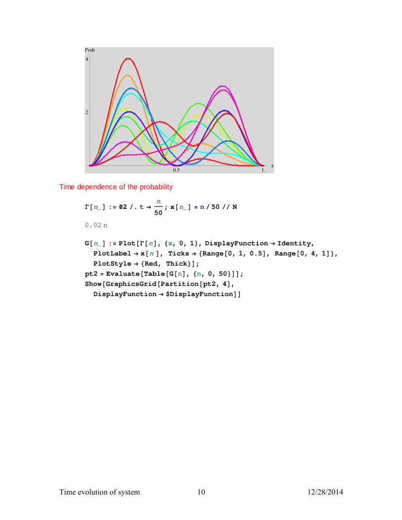
It is interesting to make a plot of P(x, t) as a function of x at various t using Mathematica' ((Mathematica)) Wave function in the One dimensional box ; time dependence of the wav e function
x_, n_ :2
aSin n x
a;
∂k_ :—2
2 m
k
a
2
;
1
6 ∂3 t
— x, 3 2 ∂2 t
— x, 2 ∂1 t
— x, 1;
rule1 m 1, — 1, a 1; 1 . rule1 Simplify;
2 Abs12;
R1 PlotEvaluateTable2, t, 0, 5, 0.5, x, 0, 1,
PlotStyle TableThick, Hue0.1 i, i, 0, 10,
Background LightGray, AxesLabel "x", "Prob",
Ticks Range0, 1, 0.5, Range0, 4, 2
Time evolution of system 10 12/28/2014
0.5 1.x
2
4
Prob
Time dependence of the probability
n_ : 2 . t n
50; xn_ n 50 N
0.02 n
Gn_ : Plotn, x, 0, 1, DisplayFunction Identity,
PlotLabel xn , Ticks Range0, 1, 0.5, Range0, 4, 1,
PlotStyle Red, Thick;
pt2 EvaluateTableGn, n, 0, 50;
ShowGraphicsGridPartitionpt2, 4,
DisplayFunction $DisplayFunction

Time evolution of system 11 12/28/2014

Time evolution of system 12 12/28/2014
Fig. Time dependence of P(t) as a function of x, at t = 0 – 0.78. 7. Example-II
Suppose that the Hamiltonian operator H is given by the matrix element of the basis
{ nb }. We assume the unitary operator U such that
nn bU .
We consider the eigenvalue problem;
nnnH ˆ ,
or
nnn bUbUH ˆˆˆ ,
or
Time evolution of system 13 12/28/2014
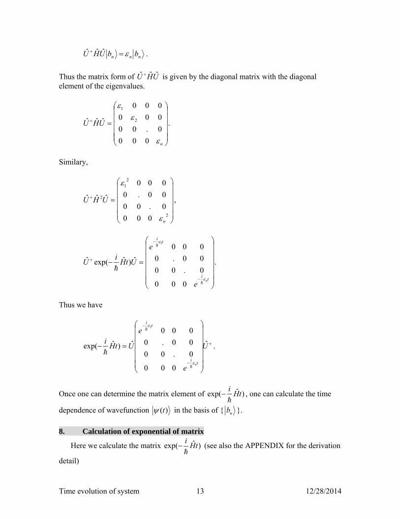
nnn bbUHU ˆˆˆ .
Thus the matrix form of UHU ˆˆˆ is given by the diagonal matrix with the diagonal element of the eigenvalues.
n
UHU
000
0.00
000
000
ˆˆˆ 2
1
.
Similary,
2
21
2
000
0.00
00.0
000
ˆˆˆ
n
UHU
,
ti
ti
n
e
e
UtHi
U
000
0.00
00.0
000
ˆ)ˆexp(ˆ
1
.
Thus we have
U
e
e
UtHi
ti
ti
n
ˆ
000
0.00
00.0
000
ˆ)ˆexp(
1
.
Once one can determine the matrix element of )ˆexp( tHi
, one can calculate the time
dependence of wavefunction )(t in the basis of { nb }.
8. Calculation of exponential of matrix
Here we calculate the matrix )ˆexp( tHi
(see also the APPENDIX for the derivation
detail)

Time evolution of system 14 12/28/2014
with
12
21H ,
in the basis of .2,1
Eigensystem[ H ].
2
12
1
1 , for the eigenvalue = 3
2
12
1
2 . for the eigenvalue = -1
The unitary operator is
2
1
2
12
1
2
1
U ,
2
1
2
12
1
2
1
U ,
ti
ti
e
e
tUHUi
UtHi
U
0
0
)ˆˆˆexp(ˆ)ˆexp(ˆ
3 ,
or

Time evolution of system 15 12/28/2014
)2
cos()2
sin(
)2
sin()2
cos(ˆ
0
0ˆ)ˆexp(3
tti
ti
t
eUe
eUtHi t
i
ti
ti
.
Note that using the Mathematica, one can directly calculate the exponential of the matrix, even if the matrix is a diagonal one. We need to use
MatrixExp[A], where A is an arbitrary matrix. ((Mathematica))

Time evolution of system 16 12/28/2014
Clear"Global`"; exp_ : exp . Complexre_, im_ Complexre, im;
H 1, 2, 2, 1; eq1 EigensystemH3, 1, 1, 1, 1, 1
1 Normalizeeq12, 1; 2 Normalizeeq12, 2; a1 eq11, 1;
a2 eq11, 2;
1.2
0
UT 1, 2 1
2,
1
2, 1
2,
1
2
U TransposeUT; UH UT; H1 UH.H.U Simplify
3, 0, 0, 1
K1 Exp —
t a1, 0, 0, Exp —
t a2 Simplify
3 t— , 0, 0,
t—
p1 U.K1.UH Expand
1
2 t—
1
23 t
— , 1
2 t—
1
23 t
— , 1
2 t—
1
2 3 t
— ,1
2 t—
1
2 3 t
—
Direct calculation for comparison
p2 MatrixExp —
t H FullSimplify
t— Cos2 t
—,
t— Sin2 t
—, t
— Sin2 t
—,
t— Cos 2 t
—
p1 p2 Simplify
0, 0, 0, 0 ________________________________________________________________________ 9. Spin precession
We consider the motion of spin S (=1/2) in the presence of an external magnetic field B along the z axis. The magnetic moment of spin is given by
ˆ z
2Bˆ S z
B
ˆ z .

Time evolution of system 17 12/28/2014
Then the spin Hamiltonian (Zeeman energy) is described by
ˆ H ˆ z B (
2Bˆ S z
)B B
ˆ z B.
Since the Bohr magneton µB is given by B
e
2mc,
BB
eB
2mc
2
eB
mc
20 (e>0).
or
0 eB
mc, (angular frequency of the Larmor precession)
Thus the Hamiltonian can be rewritten as
ˆ H
2 0
ˆ z .
Thus the Schrödinger equation is obtained as
)0(]ˆ2
exp[)0(]ˆexp[)( 0 tti
ttHi
t z
.
Note that the time evolution operator coincides with the rotation operator
ˆ R z (0t) exp[i
20
ˆ z t].
((Note)) Classical physics

Time evolution of system 18 12/28/2014
Fig. Precession motion of spin around the z axis, where the magnetic field B is applied
along the z axis.
The torque is exerted on the magnetic moment
Sμ B2
, in the form
BS
Bμτ )2
(
B .
So the spin vector S rotates around the z axis in counter-clock wise. ________________________________________________________________________ We assume that

Time evolution of system 19 12/28/2014
)2
sin(
)2
cos(]ˆ
2exp[]ˆ
2exp[)0(
2
2
i
i
yz
e
ez
iit n ,
ˆ R z (0t) exp[
i
20
ˆ z t],
The average
nn ]ˆ2
exp[]ˆ2
exp[2
)(ˆ)( 00 ti
ti
tStS zxzxtx ,
nn ]ˆ2
exp[]ˆ2
exp[2
)(ˆ)( 00 ti
ti
tStS zyzyty ,
nn ]ˆ2
exp[]ˆ2
exp[2
)(ˆ)( 00 ti
ti
tStS zzzztz .
Here we have
0
0
0
001
10
0
0]ˆ2
exp[]ˆ2
exp[
0
0
0
0
0
0
2
2
2
2
00
it
it
it
it
it
it
zxz
e
e
e
e
e
eti
ti
0
0
0
00
0
0
0]ˆ2
exp[]ˆ2
exp[
0
0
0
0
0
0
2
2
2
2
00
it
it
it
it
it
it
zyz
ie
ie
e
ei
i
e
eti
ti
10
01]ˆ
2exp[]ˆ
2exp[ 00 t
it
izzz ,
Thus we have
Time evolution of system 20 12/28/2014
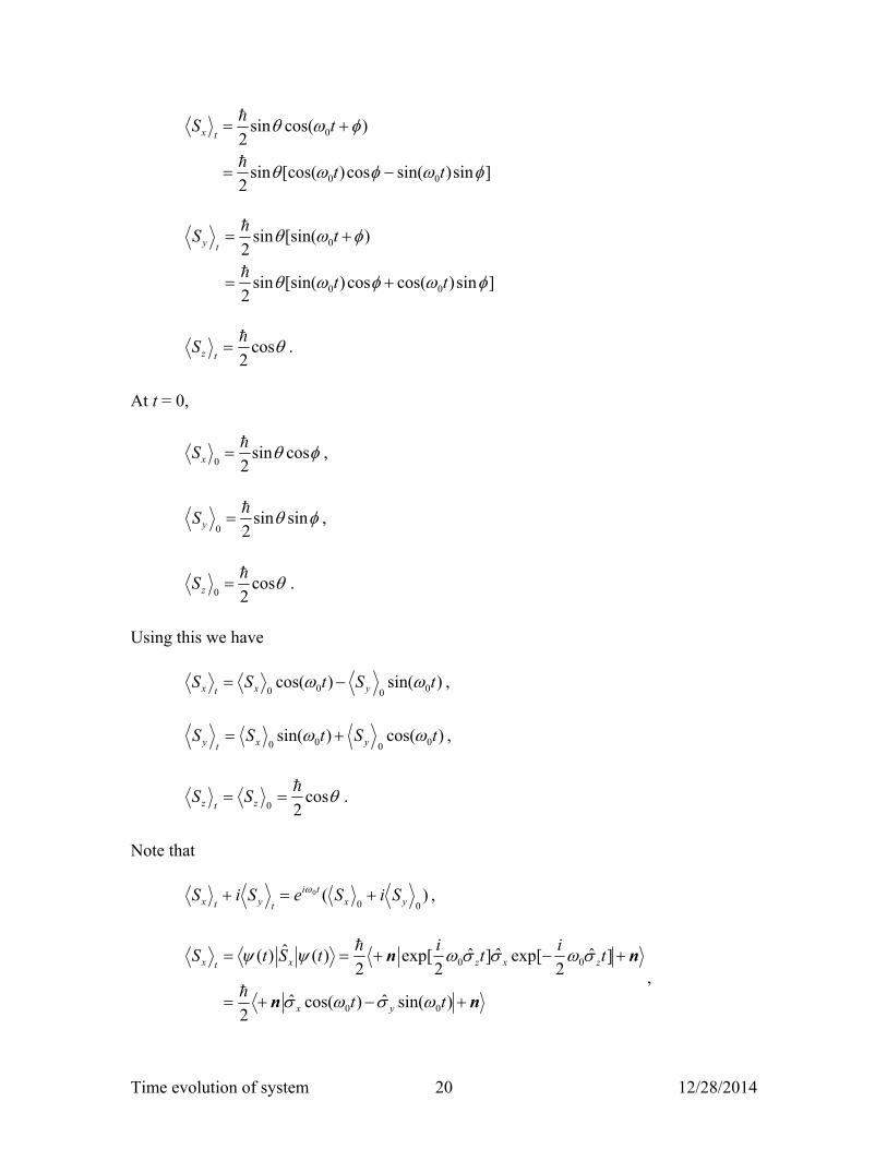
]sin)sin(cos)[cos(sin2
)cos(sin2
00
0
tt
tStx
]sin)cos(cos)[sin(sin2
)[sin(sin2
00
0
tt
tSty
cos2
tzS .
At t = 0,
cossin20
xS ,
sinsin20
yS ,
cos20
zS .
Using this we have
)sin()cos( 0000tStSS yxtx ,
)cos()sin( 0000tStSS yxty ,
cos20
ztz SS .
Note that
)(00
0yx
ti
tytx SiSeSiS ,
nn
nn
)sin(ˆ)cos(ˆ2
]ˆ2
exp[ˆ]ˆ2
exp[2
)(ˆ)(
00
00
tt
ti
ti
tStS
yx
zxzxtx
,

Time evolution of system 21 12/28/2014
where
nn xxS 20
.
We also get
nn
nn
)cos(ˆ)sin(ˆ2
]ˆ2
exp[ˆ]ˆ2
exp[2
)(ˆ)(
00
00
tt
ti
ti
tStS
yx
zyzyty
by using the Baker-Hausdorf lemma,
nn yyS 20
,
and
0
00
ˆ2
]ˆ2
exp[ˆ]ˆ2
exp[2
)(ˆ)(
zz
zzz
ztz
S
ti
ti
tStS
nn
nn
Then
)sin()cos( 0000tStSS yxtx ,
)cos()sin( 0000tStSS yxty ,
and
0ztz SS .

Time evolution of system 22 12/28/2014
q
x
y
z
________________________________________________________________________ 10 Baker- Hausdorff lemma Baker-Campbell-Hausdorff Theorem
Henry Frederick Baker, John Edward Campbell, Felix Hausdorff.
(We will discuss this theorem in the topics of coherent state and squeezed state later).
In the commutation relations, yxz JiJJ ˆ]ˆ,ˆ[ , we put zzJ 2
ˆ and xxJ
2ˆ
Then we have
yxz i ˆ2
]ˆ2
,ˆ2
[
or yxz i ˆ2]ˆ,ˆ[ .
Similarly, we have
zyx i ˆ2]ˆ,ˆ[ , xzy i ˆ2]ˆ,ˆ[ .
We notice the following relations which can be derived from the Baker-Hausdorf
lemma:

Time evolution of system 23 12/28/2014
...]]]ˆ,ˆ[,ˆ[,ˆ[!3
]]ˆ,ˆ[,ˆ[!2
]ˆ,ˆ[!1
ˆ)ˆexp(ˆ)ˆexp(32
BAAAx
BAAx
BAx
BxABxA
sinˆcosˆ]ˆ2
exp[ˆ]ˆ2
exp[ yxzxz ii ,
exp[i2
ˆ z ] ˆ y exp[i2
ˆ z ] ˆ x sin ˆ y cos .
((Proof))
We note that
2
ix , zA ˆ , and xB ˆ .
yxz iBA ˆ2]ˆ,ˆ[]ˆ,ˆ[
Then we have
]]]ˆ,ˆ[,ˆ[,ˆ[!3
]]ˆ,ˆ[,ˆ[!2
]ˆ,ˆ[!1
ˆ
]ˆexp[ˆ]ˆexp[32
xzzzxzzxzx
zxz
xxx
xxI
.....]]]]ˆ,ˆ[,ˆ[,ˆ[,ˆ[!4
4
xzzzz
x
.]]]ˆ2,ˆ[,ˆ[,ˆ[2!4
1
]]ˆ2,ˆ[,ˆ[2!3
1]ˆ2,ˆ[
2!2
1ˆ2
2!1
1ˆ
4
32
yzzz
yzzyzyx
ii
ii
ii
ii
I
or

Time evolution of system 24 12/28/2014
...]]ˆ,ˆ[,ˆ)[2)(2(2!4
1
]ˆ,ˆ)[2)(2(2!3
ˆ22
ˆˆ
]]].....ˆ,ˆ[,ˆ[,ˆ)[2(2!4
1
]]ˆ,ˆ[,ˆ)[2(2!3
]ˆ,ˆ[2
ˆˆ
4
4
3
3
2
2
4
4
3
3
2
2
xzz
xzxyx
zyzz
zyzzyyx
ii
iii
ii
i
ii
iI
or
cosˆcosˆ
...)!3
1(ˆ...)!42
1(ˆ
...ˆ!4
ˆ!3
ˆ2
ˆˆ
...ˆ)2)(2)(2)(2(2!4
1ˆ)2)(2(
2!3ˆ
2ˆˆ
342
432
4
42
3
32
yx
yx
xyxyx
xyxyx iiiiiii
I
______________________________________________________________________ 11 Schrödinger picture The Schrödinger equation
)()( tt s ,
)(),(ˆ)( 00 tttUt ss ,
where ˆ U (t, t0 ) is the time evolution operator;
ˆ U (t, t0 ) ˆ U 1(t, t0 ) .
In the Schrodinger picture, the average of the operator sA in the state )(ts is defined
by
)(ˆ)( tAt sss .
12 Heisenberg picture
The state vector, which is constant, is equal to
)()( 0tt sH .

Time evolution of system 25 12/28/2014
From the definition
sssHHH tAtA )(ˆ)(ˆ ,
or
ˆ A H(t) ˆ U ( t,t0)ˆ A s (t)
ˆ U (t,t0 ). In general, ˆ A H(t) depends on time, even if ˆ A s (t) does not. 13 Heisenberg’s equation of motion
The Schrödinger equation can be described in the Schrödinger picture
)()(ˆ)( ttHtt
i sss
,
or
)(),(ˆ)(ˆ)(),(ˆ0000 tttUtHtttU
dt
di sss ,
or
),(ˆ)(ˆ),(ˆ00 ttUtHttU
dt
di s ,
or
d
dtˆ U (t,t0 )
i
ˆ H s (t)
ˆ U (t, t0 ),
and
d
dtˆ U (t,t0 )
i
ˆ U (t, t0 ) ˆ H s (t),
where ˆ H s
(t) ˆ H s (t) . Therefore

Time evolution of system 26 12/28/2014
Hs
HH
sss
sssss
sss
H
dt
tAdtAtH
i
ttUdt
tAdttUttUtAtHttU
i
ttUdt
tAdttUttUtH
itAttUttUtAtHttU
i
ttUdt
tAdttU
dt
ttUdtAttUttUtA
dt
ttUd
dt
tAd
))(ˆ
()](ˆ),(ˆ[
),(ˆ)(ˆ),(ˆ),(ˆ)](ˆ),(ˆ)[,(ˆ
),(ˆ)(ˆ),(ˆ),(ˆ)(ˆ)(ˆ),(ˆ),(ˆ)(ˆ)(ˆ),(ˆ
),(ˆ)(ˆ),(ˆ),(ˆ
)(ˆ),(ˆ),(ˆ)(ˆ),(ˆ)(ˆ
0000
000000
000
000
where
),(ˆ)(ˆ),(ˆ)(ˆ00 ttUtHttUtH sH
.
Finally we obtain the Heisenberg’s equation of motion
i
d
dtˆ A H(t) [ ˆ A H(t), ˆ H H (t)] i(
d ˆ A s (t)
dt)H
14 Simple example for the Heisenberg picture
ˆ H s( t) ˆ H , ˆ A s (t) ˆ A , t0 = 0
tHi
eUˆ
ˆ
,
tHi
s
tHi
sH eAeUAUAˆˆ
ˆˆˆˆˆ ,
sH HH ˆˆ .
Then we have the Heisenberg’s equation of motion:
]ˆ,ˆ[ˆHHH HAA
dt
di .
We get an analogy between the classical equations of motion in the Hamiltonian form
and the quantum equations of motion in the Heisenberg’s form. HA is called a constant
of the motion, when ]ˆ,ˆ[ HH HA =0 at all times.

Time evolution of system 27 12/28/2014
UHAU
UAUUHUUHUUAUHA
SS
SSSSHH
ˆ]ˆ,ˆ[ˆ
ˆˆˆˆˆˆˆˆˆˆˆˆ]ˆ,ˆ[
Therefore ]ˆ,ˆ[ HH HA means 0]ˆ,ˆ[ SS HA
15. Ehrenfest’s theorem: Schrodinger picture Paul Ehrenfest (January 18, 1880 – September 25, 1933) was an Austrian and Dutch physicist and mathematician, who made major contributions to the field of statistical mechanics and its relations with quantum mechanics, including the theory of phase transition and the Ehrenfest theorem.
http://en.wikipedia.org/wiki/Paul_Ehrenfest ____________________________________________________________________ Schrödinger equation:
)(ˆ)( tHtt
i
or )(ˆ)( tHi
tt
.
Taking the Hermitian conjugate of both sides,
HtHttt
i ˆ)(ˆ)()(
,
or
Hti
Hti
tt
ˆ)(ˆ)()(
.
We now consider the time dependence of the average defined by )(ˆ)( tAt

Time evolution of system 28 12/28/2014
)(ˆ
)()(]ˆ,ˆ[)(
)()(ˆ)()(ˆ
)()(ˆˆ)(
))((ˆ)()(ˆ
)()(ˆ))(()()(ˆ)(
tt
AttHAt
i
ti
Attt
AttAHt
i
tt
Attt
AttAt
tttAt
dt
d
or
)(ˆ
)()(]ˆ,ˆ[)()(ˆ)( tt
AttHAt
itAt
dt
d
.
When 0ˆ
t
A, we have
)(]ˆ,ˆ[)()(ˆ)( tHAti
tAtdt
d
,
where
AHHAHA ˆˆˆˆ]ˆ,ˆ[ .
When 0]ˆ,ˆ[ HA , we get
consttAt )(ˆ)( .
16. Heisenberg’s principle of uncertainty ((Messiah, Quantum mechanics, Townsend problem (4-15) first edition of Quantum Mechanics))
Consider any observable A associated with the state of the system in quantum mechanics. Show that there is an uncertainty relation of the form
2||
Adt
dA
E ,
provided the operator A does not depend on explicitly on time. The quantity
||/ Adt
dA is a time we may call t. What is the physical significance of t.?

Time evolution of system 29 12/28/2014
((Solution)) We recall that
CiBA ˆ]ˆ,ˆ[ , implies that
2
CBA .
We start with the commutator ]ˆ,ˆ[ HA ; then
|]ˆ,ˆ[|2
1HAEA .
But since
]ˆ,ˆ[ˆ HAi
Adt
d
,
then we get
||2
Adt
dEA
,
or
2||
Adtd
AE
.
If we define
|| A
dt
dA
t
,
then
2
tE .

Time evolution of system 30 12/28/2014
For example, for position, if x = 1 cm and scmxdt
d/1.0 . then we have
dt
xdx
10 s,
which is the time necessary for x to shift by an amount x.
17. Example for the Ehrenfest theorem
We consider a particle in a stationary potential.
)ˆ(2
ˆˆ2
xVm
pH .
So that we can write
)(]ˆ
)(
)(]2
ˆ,ˆ[)(
)(]ˆ,ˆ[)()(ˆ)(
2
tm
pti
i
tm
pxt
i
tHxti
txtdt
d
or
)(]ˆ
)()(ˆ)( tmp
ttxtdtd ,
or
pm
xdtd 1
.
Similarly
)()]ˆ(ˆ
)(
)()]ˆ(,ˆ[)(
)(]ˆ,ˆ[)()(ˆ)(
txVx
ti
i
txVpti
tHpti
tptdt
d

Time evolution of system 31 12/28/2014
or
)()]ˆ(ˆ
)()(ˆ)( txVx
ttptdt
d
,
or
dxdV
pdtd
,
The equations
pm
xdt
d 1 ,
and
dx
dVp
dt
d
express the Ehrenfest’s theorem. These forms recall that of classical Hamiltonian-Jacobi equations for a particle. 18 The same example in the Heisenberg picture
)ˆ(ˆ2
1 2SSS xVp
mH , (Schrödinger picture)
HH 1
2mˆ p H
2 V( ˆ x H ), (Heisenberg’s picture)
1ˆˆˆ]ˆ,ˆ[ˆ
ˆˆˆˆˆˆˆˆˆˆˆˆ
ˆˆˆˆ]ˆ,ˆ[
iUUiUpxU
UxUUpUUpUUxU
xppxpx HHHHHH
H
HH
pi
UpUi
UpxUpx
ˆ2
ˆˆˆ2
ˆ]ˆ,ˆ[ˆ]ˆ,ˆ[ 22
Heisenberg’s equation for the free particles,

Time evolution of system 32 12/28/2014
HHH
HHHHH pim
pp
im
pxm
Hxxdt
di ˆ
2
2ˆ
ˆ2
1]ˆ,ˆ[
2
1]ˆ,ˆ[ˆ 22
,
or
d
dtˆ x H [ ˆ x H , ˆ H H ]
1
mˆ p H .
Similarly
)ˆ(ˆ
)(ˆ)]ˆ(ˆ,ˆ[ˆˆ]ˆ,ˆ[ˆ]ˆ,ˆ[ˆ HH
HHH xVx
iUxVpUUHpUHppdt
di
,
or
H
HH x
xVp
dt
dˆ
)ˆ()(ˆ
.
We consider a simple harmonics.
22 ˆ2
1)ˆ( HH xmxV ,
HH xmpdt
dˆˆ 2 .
Now consider the linear combination,
)ˆˆ()ˆˆ( HHHH pm
ixip
m
ix
dt
d
,
ti
HHH eApm
ix
ˆ)ˆˆ( ,
or
)ˆ()ˆˆ(
m
ixip
m
ix
dt
dHHH ,
ti
HHH eBpm
ix
ˆ)ˆˆ( .
where HA and HB are time-independent operators:

Time evolution of system 33 12/28/2014
)0(ˆ)0(ˆˆHHH p
m
ixA
,
)0(ˆ)0(ˆˆHHH p
m
ixB
.
Note that )0(ˆHx and )0(ˆ Hp correspond to the operators in the Schrödinger picture. From these equations, we get final results
tpm
txx HHH
sin)0(ˆ1
cos)0(ˆˆ ,
txmtpp HHH sin)0(ˆcos)0(ˆˆ .
These look to the same as the classical equation of motion. We see that Hx and Hp operators oscillate just like their classical analogue. An advantage of the Heisenberg picture is therefore that it leads to equations which are formally similar to those of classical mechanics. ((Note))
HHHHHHH
HH
H xi
xpxm
pm
Hm
pH
dt
xdx
dt
di ˆ2
2]ˆ,ˆ[
2]ˆ
2,ˆ[
1]ˆ,
ˆ[]ˆ,
ˆ[ˆ
22
22
2
2
2
,
or
HH xxdt
dˆˆ 2
2
2
,
with the initial condition
)0(ˆ1
|ˆ 0 HtH pm
xdt
d , )0(ˆ|ˆ 0 HtH xx .
The solution is
)sin(ˆ)cos(ˆˆ 21 tCtCxH ,
1ˆ)0(ˆ CxH ,

Time evolution of system 34 12/28/2014
m
pCtnCtC
dt
xd Htt
H )0(ˆˆ)](cosˆ)sin(ˆ[|ˆ
20210 .
Thus we have
m
pC H )0(ˆˆ
2 ,
and
)sin()0(ˆ
)cos()0(ˆˆ tm
ptxx H
HH
.
________________________________________________________________________ 19 Analogy with classical mechanics
In the classical mechanics, dynamical variables vary with time according to the Hamilton’s equations of motion,
j
j
p
H
dt
dq
,
where qj and pj are a set of canonical co-ordinate and momentum, and H is the Hamiltonian expressed as a function of them,
),...,,,,....,,,( 321321 nn ppppqqqqHH .
where n is the degree of freedom. For a given variable ),...,,,,....,,,( 321321 nn ppppqqqqvA ,
classical
j jjjj
j
j
j
j
j
HA
q
H
p
A
p
H
q
A
dt
dp
p
A
dt
dq
q
A
dt
dA
],[
[ ]classical:a classical definition of a Poisson bracket. 20 Dirac picture (Interaction picture)
ˆ H ˆ H 0 ˆ V s (t) ,

Time evolution of system 35 12/28/2014
where ˆ H 0 is independent of t.
)()(0
ˆ
tet I
tHi
s
,
or
)()(0
ˆ
tet s
tHi
I .
We assume that
)(ˆ)()()(ˆ)( tAtttAt sssIII .
For convenience, ˆ A s is independent of t. or
)(ˆ)()()(ˆ)(00
ˆˆ
tAttetAet ssss
tHi
I
tHi
s
,
or
s
tHi
I
tHi
AetAe ˆ)(ˆ 00ˆˆ
,
or
tHi
s
tHi
I eAetA00
ˆˆˆ)(ˆ
,
or
]ˆ),(ˆ[
]ˆˆˆˆ[)(ˆ
0
0
ˆˆˆˆ
0
0000
HtA
HeAeeAeHi
itAdt
di
I
tHi
s
tHi
tHi
s
tHi
I
.
Thus every operator behaves as if it would in the Heisenberg representation for a non-interacting system.

Time evolution of system 36 12/28/2014
)()(ˆ
)()(
00
0
ˆˆ
0
ˆ
tt
ieteH
tet
itt
i
s
tHi
s
tHi
s
tHi
I
Since
)()](ˆˆ[)( 0 ttVHtt
i sss
,
)()](ˆˆ[)(ˆ)()( 0
ˆˆ
0
ˆ000
ttVHeteHtet
itt
i s
tHi
s
tHi
s
tHi
I
,
or
)()(ˆ)()(ˆ)(00
ˆˆ
ttVtetVett
i III
tHi
tHi
I
,
or
)()(ˆ)( ttVtt
i III
,
where
tHi
s
tHi
I etVtV00
ˆˆ
)(ˆ)(ˆ
(Schrödinger-like)
which is a Schrödinger equation with the total ˆ H replaced by ˆ V I . We assume that
)(),(ˆ)( 00 tttUt III ,
satisfies the equation
)()(ˆ)( ttVtt
i III
.
Then we have the following relation.
),(ˆ)(ˆ),(ˆ00 ttUtVttU
ti III
,

Time evolution of system 37 12/28/2014
with the initial condition
'),'(ˆ)'(ˆ1),(ˆ
0
00 dtttUtVi
ttUt
t
III
.
We can obtain an approximate solution to this equation [Dyson series].
t
t
t
t
II
t
t
I
t
t
t
t
IIII
tVtVdtdti
dttVi
dtdtttUtVi
tVi
ttU
0 00
0 0
'2
'
00
...)''(ˆ)'(ˆ"')(')'(ˆ)(1
']"),"(ˆ)''(ˆ1)['(ˆ1),(ˆ
21 Transition probability
Once ˆ U I (t, t0 ) is given we have
)(),(ˆ)( 00 tttUt III ,
where
)()(0
ˆ
tet I
tHi
s
, or )()(0
ˆ
tet s
tHi
I ,
and
)(),(ˆ)( 00 tttUt ss ,
)(),(ˆ
)(),(ˆ)(
0
ˆ
0
ˆ
00
ˆ
000
0
tettUe
tttUet
I
tHi
s
tHi
ss
tHi
I
Then we have
ˆ U I (t, t0 ) e
i
H 0t ˆ U s (t, t0 )e
i
H 0t 0
. Let us now look at the matrix element of ˆ U I (t, t0 )
nEnH n0ˆ ,

Time evolution of system 38 12/28/2014
mttUnemttUn s
tEtEi
I
mn
),(ˆ),(ˆ0
)(
0
0 ,
2
0
2
0 ),(ˆ),(ˆ mttUnmttUn sI .
((Remark)) When
0]ˆ,ˆ[ 0 AH and 0]ˆ,ˆ[ 0 BH ,
'''ˆ aaaA and '''ˆ bbbB ,
in general,
2
0
2
0 '),(ˆ''),(ˆ' attUbattUb sI .
Because
mns
tEtEi
mn
tHi
s
tHi
I
ammttUnnbe
aettUnnebattUb
mn
,0
)(
,
ˆ
0
ˆ
0
'),(ˆ'
'),(ˆ''),(ˆ'
0
000
_______________________________________________________________________ 22. Application of Schrödinger and Heisenberg pictures to simple harmonics
tHi
eUˆ
ˆ
. The operator in the Heisenberg picture is defined by
tHi
s
tHi
sH eAeUAUAˆˆ
ˆˆˆˆˆ ,
where H is the Hamiltonian
2202 ˆ
2ˆ
2
1ˆ xm
pm
H
.
Using the equation of Heisenberg picture, we obtain

Time evolution of system 39 12/28/2014
tpm
txxH
sinˆ1
cosˆˆ ,
and
txmtppH sinˆcosˆˆ . The matrix of x and p are given by
04000
40300
03020
00201
00010
2
1ˆ
x ,
and
04000
40300
03020
00201
00010
2ˆ 0
i
mp ,
((Discussion)) What are the expectation values )(ˆ)( txt and )(ˆ)( tpt ?
tpm
tx
tpm
tx
xtxt H
sin)0(ˆ)0(1
cos)0(ˆ)0(
)0(sinˆ1
cosˆ)0(
)0(ˆ)0()(ˆ)(
Time evolution of system 40 12/28/2014
txmtp
txmtp
ptpt H
sin)0(ˆ)0(cos)0(ˆ)0(
)0(sinˆcosˆ)0(
)0(ˆ)0()(ˆ)(
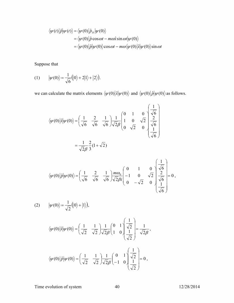
Suppose that
(1) 21206
1)0( .
we can calculate the matrix elements )0(ˆ)0( x and )0(ˆ)0( p as follows.
)21(3
2
2
1
6
16
26
1
020
201
010
2
1
6
1
6
2
6
1)0(ˆ)0(
x
0
6
16
26
1
020
201
010
26
1
6
2
6
1)0(ˆ)0( 0
i
mp
,
(2) 102
1)0( ,
2
1
2
12
1
01
10
2
1
2
1
2
1)0(ˆ)0(
x ,
0
2
12
1
01
10
2
1
2
1
2
1)0(ˆ)0(
p ,

Time evolution of system 41 12/28/2014
ttxt
cos2
1)(ˆ)( ,
and
tm
tpt sin
2)(ˆ)( .
((Another method, Schrödinger picture))
/
/
//
/ˆ
1
0
10
2
1
102
1
102
1)(
tiE
tiE
tiEtiE
tHi
e
e
ee
et
// 10
2
1)( tiEtiEet ,
tee
e
ee
e
eetxt
titi
tiE
tiEtiEtiE
tiE
tiEtiEtiE
0
/
///
/
///
2
cos2
1)(
2
1
2
1
2
1
2
1
01
10
2
1
2
1)(ˆ)(
00
0
1
10
1
0
10
________________________________________________________________________ 23. Example-1
A spin 1/2 particles in a eigenstate of Sx, with eigenvalue 2/ at time t = 0. At that time it is placed in a magnetic field of magnitude B pointing in the z direction, in which it is allowed to precess for a time T. At that instant, the magnetic field is rotated very rapidly, so that it is now points in the y direction. After another time interval T, a measurement of Sx is carried. What is the probability that the value 2/ will be found? ((Solution)) The spin has a spin magnetic moment.

Time evolution of system 42 12/28/2014
σσSμ ˆˆ2
2ˆ2ˆ B
BB
.
The spin Hamiltonian in the presence of the magnetic field B,
nσnσnσBσBμ
ˆ
2
1ˆ
2
1ˆ
2ˆˆˆ
0
mc
eB
mc
BeH B ,
where n is the unit vector along the direction of B, and 0 is the Larmor angular
frequency. Note that the period 0T is expressed by 0
0
2
T
At t = 0, we have xt 0( .
For 0≤t≤T, the magnetic field is applied along the z direction.
zH ˆ2
1ˆ0
we have
)0()ˆ2
exp()0()ˆ
exp()( 0 tti
tHit
t z
,
and
xT
TRx
T
Tit
TiTt zzz )2(ˆ)ˆexp()0()ˆ
2exp()(
00
0 .
where )(ˆ zR is the rotation operator around the z axis by the angle . For T≤t≤2T, the magnetic field is applied along the y direction.
yH ˆ2
1ˆ0
we have
)()ˆ2
)(exp(
)()ˆ)(
exp()(
0 TtTti
TtHTti
t
y

Time evolution of system 43 12/28/2014
xT
TR
T
TR
TtT
Ti
TtTi
Tt
zy
y
y
)2(ˆ)2(ˆ
)()ˆexp(
)()ˆ2
exp()2(
00
0
0
Now we calculate
xRRx
xT
TR
T
TRxTtx
zy
zy
)(ˆ)(ˆ
)2(ˆ)2(ˆ)2(00
where
0
2T
T .
Using the formula
)2
sin()ˆ(1)2
cos()ˆ2
exp()(ˆ nnn iiR ,
2
2
0
0)2
sin(ˆ1)2
cos()(ˆ
i
i
zz
e
eiR ,
2cos
2sin
2sin
2cos
)2
sin(ˆ1)2
cos()(ˆ
yy iR .
Note that
1
1
2
1x

Time evolution of system 44 12/28/2014
2
12
1
0
0
2cos
2sin
2sin
2cos
2
1
2
1)2(
2
2
i
i
e
eTtx
or
)2cos2(4
1)2( i
iTtx
Then the probability is given by
)]2(cos1[2
1]cos1[
2
1)2cos2(
4
1)2(
0
222
0 T
Ti
i
T
TP
24. Example-2
A particle with intrinsic spin one is placed in a constant external magnetic field B0 in
the x direction. The initial spin state of the particle is 1,11,1)0( ml , that is,
a state with Sz . Take the spin Hamiltonian to be
ˆ H 0ˆ J x ,
and determine the probability P(t) that the particle is in the state 1,1 at time t. Make a
plot of P(t) as a function of time t (0≤0t≤2π). Hint: x
1,1 , x
0,1 , and x
1,1 are the
eigenket of ˆ H . ((Solution))
zxJt
itHi
t 1,1)ˆexp()0()ˆexp()( 0
For simplicity, hereaftre we use
.1,11,1 z
Noting that
xxx1,1
2
10,1
2
11,1
2
11,1
we get

Time evolution of system 45 12/28/2014
xxx
xxxx
x
titi
Jt
i
Jt
it
1,1)exp(2
10,1
2
11,1)exp(
2
1
]1,12
10,1
2
11,1
2
1)[ˆexp(
1,1)ˆexp()(
00
0
0
The probability P(t) is given by
2
00
21,11,1)exp(
2
10,11,1
2
11,11,1)exp(
2
1)(1,1)(
xxxtitittP
Then we have
2sin)cos1(
4
1
)exp(4
1
2
1)exp(
4
1
)(1,1)(
0420
2
00
2
tt
titi
ttP
0 p4
p2
3 p4
p5 p4
3 p2
7 p4
2 p
w0t
0.2
0.4
0.6
0.8
1.0
Pt
((Note))

Time evolution of system 46 12/28/2014
xxxxU 1,1
2
10,1
2
11,1
2
1
2
12
12
1
0
0
1
2
1
2
1
2
12
10
2
12
1
2
1
2
1
1,1ˆ1,1
0
0
1
1,1z
,
0
1
0
0,1z
,
1
0
0
1,1z
1
2
1
2
11,1
x,
1
0
1
2
10,1
x,
1
2
1
2
11,1
x
with the unitary operator,
2
1
2
1
2
12
10
2
12
1
2
1
2
1
ˆxU ,
2
1
2
1
2
12
10
2
12
1
2
1
2
1
ˆxU
25. Example-3
Let |1> and |2> be eigenstates of a Hermitian operator ˆ A with eigenvalues a1 and a2, respectively (a1 ≠ a2). The Hamiltonian operator is given by
H = |1><2| + |2><1| or
xH
ˆ
0
0ˆ
where is just a real number.
Time evolution of system 47 12/28/2014
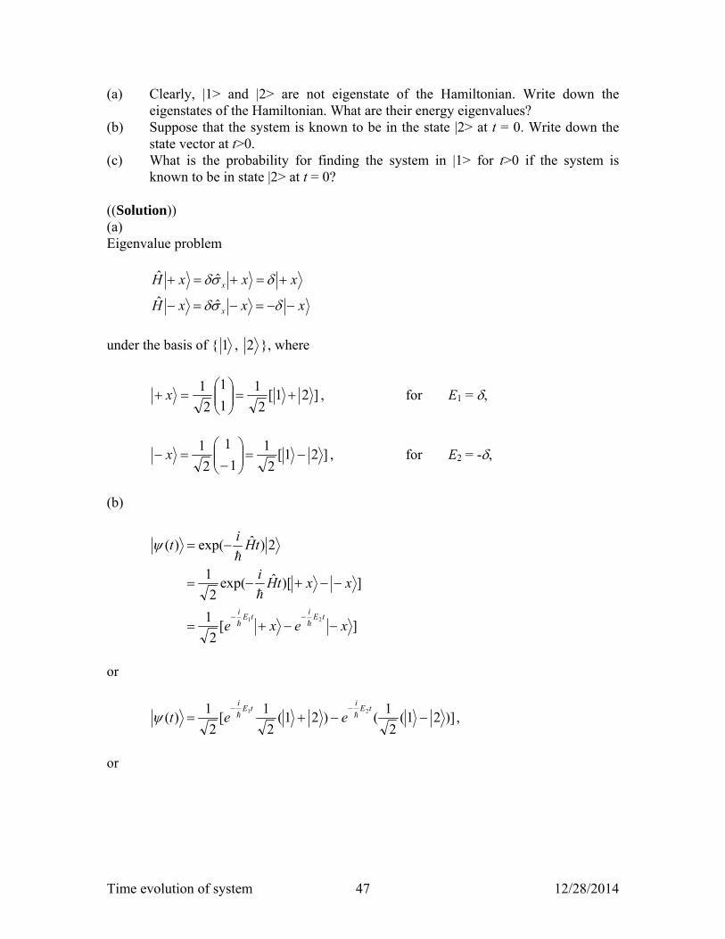
(a) Clearly, |1> and |2> are not eigenstate of the Hamiltonian. Write down the eigenstates of the Hamiltonian. What are their energy eigenvalues?
(b) Suppose that the system is known to be in the state |2> at t = 0. Write down the state vector at t>0.
(c) What is the probability for finding the system in |1> for t>0 if the system is known to be in state |2> at t = 0?
((Solution)) (a) Eigenvalue problem
xxxH
xxxH
x
x
ˆˆ
ˆˆ
under the basis of { 1 , 2 }, where
]21[2
1
1
1
2
1
x , for E1 = ,
]21[2
1
1
1
2
1
x , for E2 = -,
(b)
][2
1
])[ˆexp(2
1
2)ˆexp()(
21
xexe
xxtHi
tHi
t
tEi
tEi
or
)]21(2
1()21(
2
1[
2
1)(
21
tE
itE
i
eet ,
or
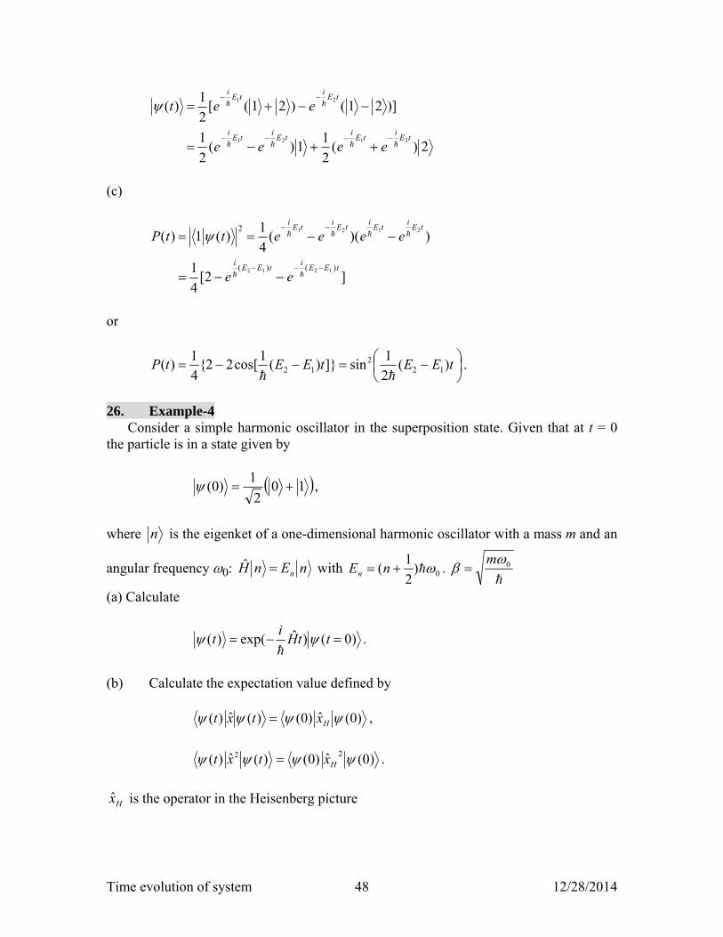
Time evolution of system 48 12/28/2014
2)(2
11)(
2
1
)]21()21([2
1)(
2121
21
tEi
tEi
tEi
tEi
tEi
tEi
eeee
eet
(c)
]2[4
1
))((4
1)(1)(
)()(
2
1212
2121
tEEi
tEEi
tEi
tEi
tEi
tEi
ee
eeeettP
or
tEEtEEtP )(
2
1sin]})(
1cos[22{
4
1)( 12
212
.
26. Example-4
Consider a simple harmonic oscillator in the superposition state. Given that at t = 0 the particle is in a state given by
102
1)0( ,
where n is the eigenket of a one-dimensional harmonic oscillator with a mass m and an
angular frequency 0: nEnH nˆ with 0)2
1( nEn .
0 m
(a) Calculate
)0()ˆexp()( ttHi
t
.
(b) Calculate the expectation value defined by
)0(ˆ)0()(ˆ)( Hxtxt ,
)0(ˆ)0()(ˆ)( 22 Hxtxt .
Hx is the operator in the Heisenberg picture

Time evolution of system 49 12/28/2014
tpm
txxH 00
0 sinˆ1
cosˆˆ
.
04000
40300
03020
00201
00010
2
1ˆ
x ,
04000
40300
03020
00201
00010
2ˆ 0
i
mp
((Heisenberg picture)) Simple harmonics
tHi
eUˆ
ˆ
. The operator in the Heisenberg picture is defined by
tHi
s
tHi
sH eAeUAUAˆˆ
ˆˆˆˆˆ ,
where H is the Hamiltonian
2202 ˆ
2ˆ
2
1ˆ xm
pm
H
.
Using the equation of Heisenberg picture, we obtain
tpm
txxH 00 sinˆ1
cosˆˆ
,
and
txmtppH 00 sinˆcosˆˆ .
Time evolution of system 50 12/28/2014
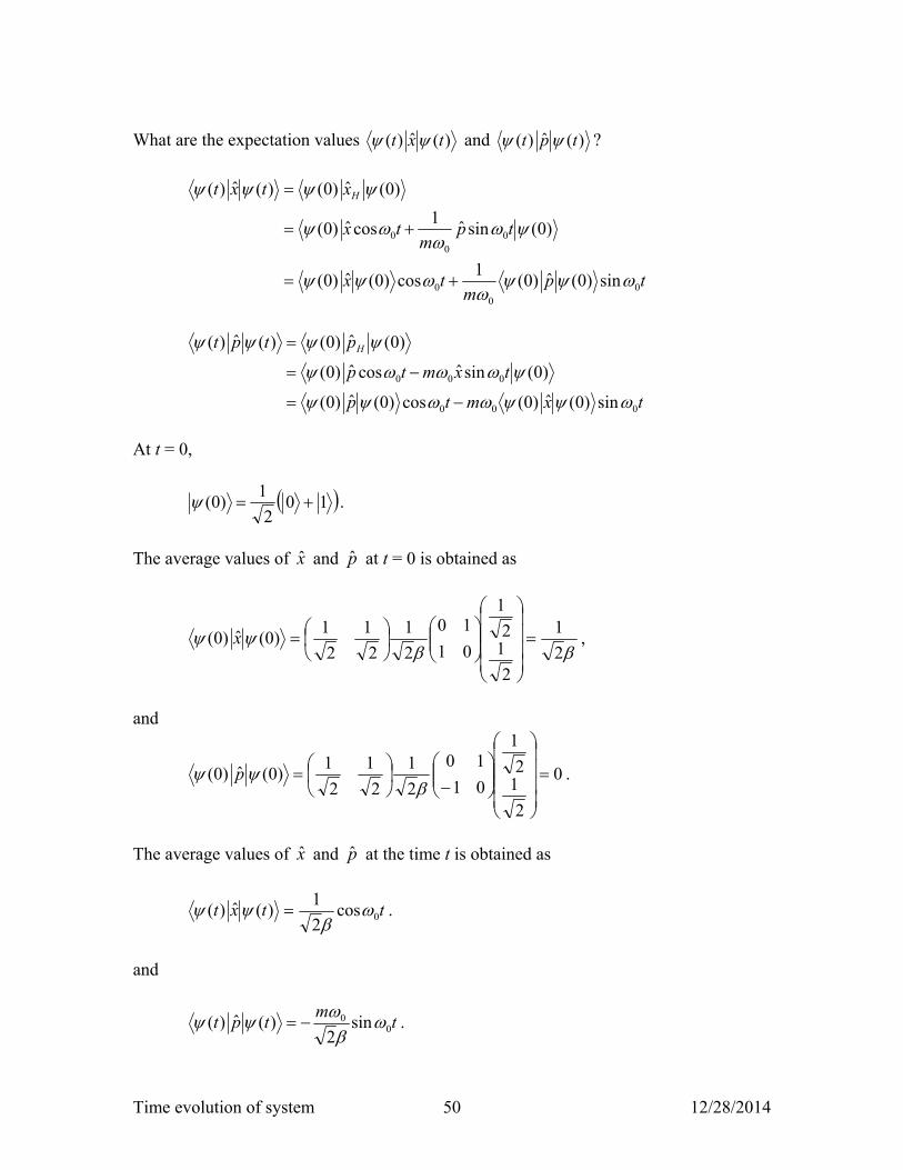
What are the expectation values )(ˆ)( txt and )(ˆ)( tpt ?
tpm
tx
tpm
tx
xtxt H
00
0
00
0
sin)0(ˆ)0(1
cos)0(ˆ)0(
)0(sinˆ1
cosˆ)0(
)0(ˆ)0()(ˆ)(
txmtp
txmtp
ptpt H
000
000
sin)0(ˆ)0(cos)0(ˆ)0(
)0(sinˆcosˆ)0(
)0(ˆ)0()(ˆ)(
At t = 0,
102
1)0( .
The average values of x and p at t = 0 is obtained as
2
1
2
12
1
01
10
2
1
2
1
2
1)0(ˆ)0(
x ,
and
0
2
12
1
01
10
2
1
2
1
2
1)0(ˆ)0(
p .
The average values of x and p at the time t is obtained as
ttxt 0cos2
1)(ˆ)(
.
and
tm
tpt 00 sin
2)(ˆ)(
.

Time evolution of system 51 12/28/2014
((Schrödinger picture))
In this picture )(t is obtained as
/
////ˆ
1
0
10
2
110
2
110
2
1)(
tiE
tiEtiEtiEtHi
e
eeeet .
Since
// 10
2
1)( tiEtiEet ,
we have
tee
e
ee
e
eetxt
titi
tiE
tiEtiEtiE
tiE
tiEtiEtiE
0
/
///
/
///
2
cos2
1)(
2
1
2
1
2
1
2
1
01
10
2
1
2
1)(ˆ)(
00
0
1
10
1
0
10
tm
eei
m
e
ee
i
m
e
ee
i
mtpt
titi
tiE
tiEtiEtiE
tiE
tiEtiEtiE
00
0
/
///0
/
///0
2
sin2
)(22
1
22
1
01
10
22
1)(ˆ)(
00
0
1
10
1
0
10
________________________________________________________________________ 27. Example-5: Cohen-Tannoudji (4-2) Consider a spin 1/2 particle. a. At time t = 0, we measure Sy and find 2/ . What is the state vector )0(
immediately after the measurement? b. Immediately after this measurement, we apply a uniform time-dependent field
parallel to the z axis. The Hamiltonian operator of the spin )(ˆ tH is then written:

Time evolution of system 52 12/28/2014
zSttH ˆ)()(ˆ0 .
Assume that )(0 t is zero for t<0 and t>T and increases linearly from 0 to 0
when Tt 0 (T is a given parameter whose dimensions are those of time). Show that at time t the state vector can be written as
][2
1)( )()( ziezet titi ,
where )(t is a real function of t.
c. At a time t = >T. we measure Sy. What results can we find, and with what probabilities? Determine the relation which must exist between 0 and T in order for us to be sure of the result. Give the physical interpretation.
((Solution)) (a)
][2
1)0( zizyt .
(b)
zSttH ˆ)()(ˆ0 .
Schrodinger equation
)(ˆ)()()(ˆ)( 0 tStttHtt
i z
.
Suppose that
)0()(ˆ)( ttUt .
)(ˆ tU satisfies the differential equation
)(ˆˆ)()(ˆ)(ˆ)(ˆ tUSttUtHtUt
i z
.
The solution is
)')'(ˆexp()(ˆ0t
dttHi
tU
.

Time evolution of system 53 12/28/2014
)(ˆ tH is time-dependent but )(ˆ tH 's at different times commute.
]ˆ)(1
exp[]')'(1ˆexp[)(ˆ
0
0
0 z
t
z StidttSitU
,
where
t
dttt0
00 ')'()( .
Then we get
][2
1
][2
1
]][ˆ)(1
exp[2
1
]ˆ)(1
exp[
)0(]ˆ)(1
exp[)(
)()(
)(2
1)(
2
1
0
0
0
00
zieze
zieze
zizSti
ySti
tStit
titi
titi
z
z
z
where
t
dtttt0
00 ')'(2
1)(
2
1)( .
')'( 00 t
Tt
for Tt '0 ,
0)'(0 t . for t'<0 and t'>T.
(c) At Tt ,
TdttT
dtttTT
0
0
0
0
0 4
1''
2
1')'(
2
1)( .

Time evolution of system 54 12/28/2014
Now we measure yS at t.
)()(
)(
)(
2
1
2
1
2
2
1
12
1)( titi
ti
ti
eee
i
eity
.
The probability
))]2
cos(1[2
1))](2cos(1[
2
1)( 02 T
ttyP .
)]2
cos(1[2
1))](2cos(1[
2
1)( 02 T
ttyP .
When 20 T , 0P , 1P .
When 40 T , 1P , 0P .
_______________________________________________________________________ REFERENCES 1. J.J. Sakurai and J. Napolitano, Modern Quantum Mechanics, second edition
(Addison-Wesley, New York, 2011). ISBN 978-0-8053-8291-4 2. John S. Townsend, A Modern Approach to Quantum Mechanics, second edition
(University Science Books, 2012). ISBN 978-1-891389-78-8 3. Claude Cohen-Tannoudji, Bernard Diu, and Franck Laloë, Quantum Mechanics
volume I and volume II (John Wiley & Sons, New York, 1977). 4. Ramamurti Shankar, Principles of Quantum Mechanics, second edition (Springer,
New York, 1994). ISBN 0-306-44790-8. 5. Schaum's Outline of Theory and Problems of Quantum Mechanics, Yoav Peleg,
Reuven, and Elyahu Zaarur (McGraw-Hill, New York, 1998). ISBN 0-07-054018-7
6. Nouredine Zettili, Quantum Mechanics, Concepts and Applications, 2nd edition (John Wiley & Sons, New York, 2009). ISBN 0-471 48943 3.
________________________________________________________________________ APPENDIX-I Calculation of exponential of matrix A.1 Example-1
Time evolution of system 55 12/28/2014
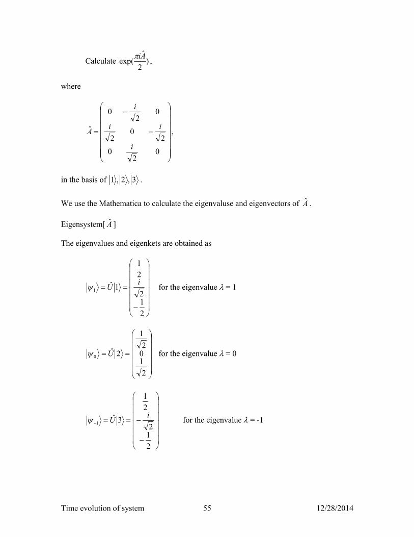
Calculate )2
ˆexp(
Ai,
where
02
0
20
2
02
0
ˆ
i
ii
i
A ,
in the basis of 3,2,1 .
We use the Mathematica to calculate the eigenvaluse and eigenvectors of A .
Eigensystem[ A ] The eigenvalues and eigenkets are obtained as
2
12
2
1
1ˆ1
iU for the eigenvalue = 1
2
102
1
2ˆ0 U for the eigenvalue = 0
2
12
2
1
3ˆ1
iU for the eigenvalue = -1

Time evolution of system 56 12/28/2014
2
1
2
1
2
12
02
2
1
2
1
2
1
ˆ iiU ,
2
1
22
12
10
2
12
1
22
1
ˆ
i
i
U .
The calculation is as follows.
2
1
2
1
2
12
10
2
12
1
2
1
2
1
ˆ
00
010
00ˆ
ˆ33)2
exp(22)02
exp(11)2
[exp(ˆ
)2
exp()02
exp()2
exp(
))(2
ˆexp()
2
ˆexp(
2/
2/
332211
110011
U
e
e
U
Uiii
U
iii
AiAi
i
i
since
11 1 A , 22 0 A , 33 )1( A .
The above result can be also obtained using the Mathematica. ((Mathematica))

Time evolution of system 57 12/28/2014
Calculate the exponent of the Matrix
Clear"Global`";
exp_ : exp . Complexre_, im_ Complexre, im;
A 1
20, , 0, , 0, , 0, , 0;
eq1 EigensystemA1, 1, 0, 1, 2 , 1, 1, 2 , 1, 1, 0, 1
a1 eq11, 2; a2 eq11, 3; a3 eq11, 1;
1 Normalizeeq12, 21
2,
2,
12
2 Normalizeeq12, 3 1
2, 0,
1
2
3 Normalizeeq12, 11
2,
2,
12
eq2 1. 2, 2. 3 , 3. 2 Simplify
0, 0, 0
UT 1, 2, 3; U TransposeUT; UH UT;
A1 UH.A.U
1, 0, 0, 0, 0, 0, 0, 0, 1
R Exp a1
2, 0, 0, 0, Exp a2
2, 0, 0, 0, Exp a3
2
Simplify
, 0, 0, 0, 1, 0, 0, 0,
Time evolution of system 58 12/28/2014
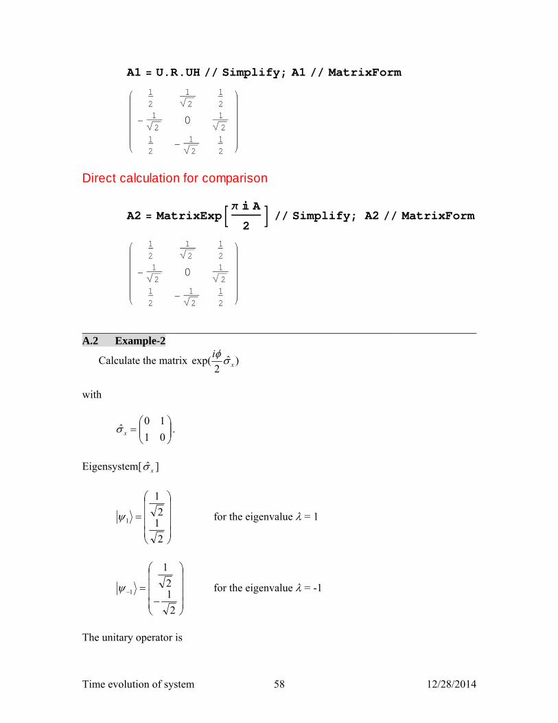
A1 U.R.UH Simplify; A1 MatrixForm
12
12
12
12
0 12
12
12
12
Direct calculation for comparison
A2 MatrixExp A
2 Simplify; A2 MatrixForm
12
12
12
12
0 12
12
12
12
________________________________________________________________________ A.2 Example-2
Calculate the matrix )ˆ2
exp( x
i
with
01
10ˆ x .
Eigensystem[ x ]
2
12
1
1 for the eigenvalue = 1
2
12
1
1 for the eigenvalue = -1
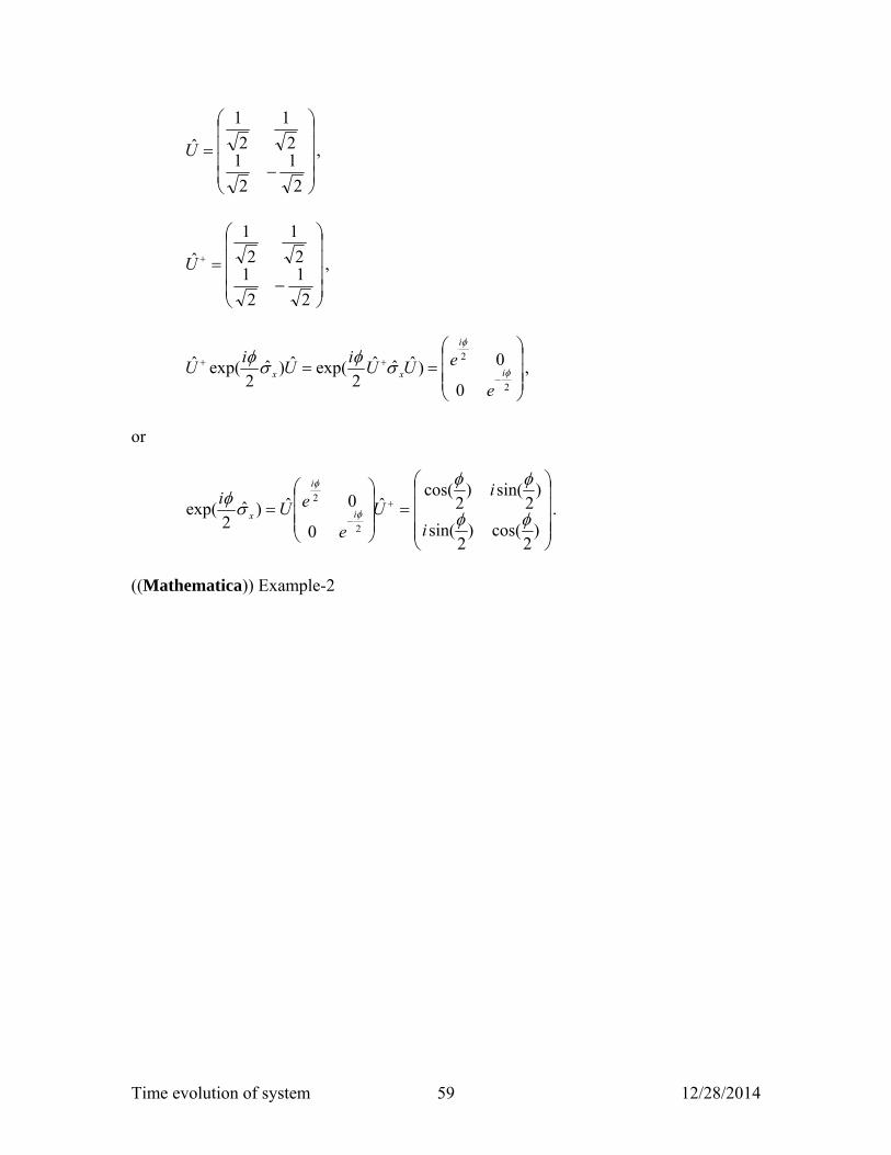
The unitary operator is
Time evolution of system 59 12/28/2014
2
1
2
12
1
2
1
U ,
2
1
2
12
1
2
1
U ,
2
2
0
0)ˆˆˆ2
exp(ˆ)ˆ2
exp(ˆ
i
i
xx
e
eUUi
Ui
U ,
or
)
2cos()
2sin(
)2
sin()2
cos(ˆ
0
0ˆ)ˆ2
exp(2
2
i
iU
e
eUi
i
i
x .
((Mathematica)) Example-2

Time evolution of system 60 12/28/2014
Clear"Global`";
exp_ : exp . Complexre_, im_ Complexre, im;
x 0, 1, 1, 0;
eq1 Eigensystemx1, 1, 1, 1, 1, 1
a1 eq11, 2; a2 eq11, 1; 1 Normalizeeq12, 2;
2 Normalizeeq12, 1;
1.2
0
UT 1, 2; U TransposeUT; UH UT;
W1 UH.x.U
1, 0, 0, 1A1 Expa1
2, 0, 0, Expa2
2 Simplify;
A1 MatrixForm
2 0
0
2
A2 U.A1.UH ExpToTrig Simplify; A2 MatrixForm
Cos 2 Sin
2
Sin 2 Cos
2
Direct cxalculation for comparison
A3 MatrixExp
2x Simplify; A3 MatrixForm
Cos 2 Sin
2
Sin 2 Cos
2