TIMBER SUPPLY ANALYSIS DATA PACKAGE
98
GOLDEN TSA TIMBER SUPPLY REVIEW # 4 TIMBER SUPPLY ANALYSIS DATA PACKAGE With updates to Nov 22, 2008 Prepared for Golden DFAM Group Louisiana Pacific . Downie Timber . BC Timber Sales . Prepared by Reg Davis, RPF Forsite Consulting Ltd.
Transcript of TIMBER SUPPLY ANALYSIS DATA PACKAGE

GOLDEN TSA TIMBER SUPPLY REVIEW # 4
TIMBER SUPPLY ANALYSIS
DATA PACKAGE
With updates to Nov 22, 2008
Prepared for
Golden DFAM Group
Louisiana Pacific .
Downie Timber .
BC Timber Sales .
Prepared by
Reg Davis, RPF
Forsite Consulting Ltd.

TABLE OF CONTENTS 1.0 INTRODUCTION...............................................................................................................................1
2.0 INVENTORY AND MODEL FILES ...................................................................................................4
3.0 LANDBASE AND INVENTORIES....................................................................................................6
3.1.1 FIP-type forest inventory ..........................................................................................................................6 3.1.2 VRI-type forest inventory..........................................................................................................................6
4.0 EXCLUSIONS FROM THE TIMBER HARVESTING LAND BASE...............................................10
4.9.1 Non-merchantable / low site ...................................................................................................................16 4.9.2 Problem Forest Types ............................................................................................................................17
4.10.1 HLPO caribou habitat requirements...................................................................................................17 4.10.2 SARCO caribou habitat requirements ................................................................................................17
4.14.1 Biodiversity – Wildlife Tree Retention Areas ......................................................................................20 4.14.2 Old Seral and Mature-plus-old Seral ..................................................................................................20
4.16.1 Future wildlife tree retention areas .....................................................................................................21 4.16.2 Future roads, trails and landings........................................................................................................21
4.18.1 Age Class distribution ........................................................................................................................22 5.0 INVENTORY AGGREGATION.......................................................................................................25
6.0 GROWTH AND YIELD ...................................................................................................................27
6.1.1 Site curves .............................................................................................................................................27 6.1.2 Site index adjustments ...........................................................................................................................27
6.4.1 Standard Operational Adjustment Factors..............................................................................................28
6.6.1 Methodology...........................................................................................................................................28 6.6.2 Existing timber volume check .................................................................................................................29
1.1 PURPOSE........................................................................................................................................11.2 PROCESS........................................................................................................................................2
2.1 BASE CASE OPTION - OVERVIEW......................................................................................................4
3.1 FOREST COVER INVENTORY.............................................................................................................6
3.2 FOREST RESOURCE INVENTORIES ....................................................................................................8
4.1 NON-CONTRIBUTING ADMINISTRATIVE CLASSES ...............................................................................124.2 NON-PRODUCTIVE AND NON-FOREST AREA......................................................................................124.3 NON-COMMERCIAL COVER..............................................................................................................134.4 ROADS TRAILS AND LANDINGS ........................................................................................................144.5 UNCLASSIFIED ROADS, TRAILS AND LANDINGS .................................................................................144.6 PARKS AND PROTECTED AREAS .....................................................................................................144.7 INOPERABLE / INACCESSIBLE..........................................................................................................154.8 UNSTABLE TERRAIN AND ENVIRONMENTALLY SENSITIVE AREAS ........................................................154.9 NON-MERCHANTABLE / LOW SITE AND PROBLEM FOREST TYPES ......................................................16
4.10 WILDLIFE: CARIBOU HABITAT..........................................................................................................17
4.11 CULTURAL HERITAGE AND ARCHAEOLOGICAL REDUCTIONS ..............................................................184.12 RIPARIAN RESERVES AND MANAGEMENT ZONES – STREAMS.............................................................184.13 RIPARIAN RESERVES AND MANAGEMENT ZONES – WETLANDS AND LAKES..........................................194.14 BIODIVERSITY................................................................................................................................20
4.15 PERMANENT SAMPLE PLOTS ...........................................................................................................204.16 FUTURE LAND BASE REDUCTIONS..................................................................................................21
4.17 AREA ADDITIONS............................................................................................................................224.18 DESCRIPTIONS OF THE LANDBASE ..................................................................................................22
5.1 ANALYSIS UNITS............................................................................................................................25
6.1 SITE INDEX....................................................................................................................................27
6.2 UTILIZATION LEVEL ........................................................................................................................276.3 DECAY, WASTE AND BREAKAGE FOR NATURAL STANDS.....................................................................276.4 OPERATIONAL ADJUSTMENT FACTORS FOR MANAGED STANDS..........................................................28
6.5 VOLUME REDUCTIONS....................................................................................................................286.6 YIELD TABLE DEVELOPMENT – NATURAL STANDS ............................................................................28
6.7 YIELD TABLE DEVELOPMENT - MANAGED STANDS .............................................................................30

ii
6.7.1 Silviculture management regimes ..........................................................................................................30 6.7.2 Regeneration delay ................................................................................................................................30 6.7.3 Stand rehabilitation.................................................................................................................................30 6.7.4 Genetic improvement .............................................................................................................................30 6.7.5 Planting Density .....................................................................................................................................32 6.7.6 TIPSY managed stand yield table inputs................................................................................................33
7.0 SILVICULTURE ..............................................................................................................................35 7.1.1 Existing managed stands .......................................................................................................................35 7.1.2 Backlog and current non-stocked area (NSR) ........................................................................................35
8.0 UNSALVAGED LOSSES ...............................................................................................................36 9.0 RESOURCE MANAGEMENT ........................................................................................................37
9.1.1 Forest Cover Requirements ...................................................................................................................37 9.1.2 Visual Resources ...................................................................................................................................39 9.1.3 Recreation resources .............................................................................................................................40 9.1.4 Wildlife....................................................................................................................................................41 9.1.5 Biodiversity .............................................................................................................................................42 9.1.6 Domestic Watersheds ............................................................................................................................47 9.1.7 Lakeshore, wetland and riparian management zones ............................................................................47
9.2.1 Minimum harvesting age / merchantability standards.............................................................................47 9.2.2 Operability / harvest systems .................................................................................................................49 9.2.3 Initial Harvest Rate .................................................................................................................................49 9.2.4 Harvest rules ..........................................................................................................................................49 9.2.5 Harvest profile ........................................................................................................................................49 9.2.6 Silviculture Systems ...............................................................................................................................49 9.2.7 Harvest flow objectives...........................................................................................................................50
10.0 TIMBER SUPPLY MODELING AND FORECASTS ......................................................................51
10.6.1 Old growth management areas..........................................................................................................53 10.6.2 Caribou management areas...............................................................................................................53
10.7.1 Attack Priority.....................................................................................................................................55 10.7.2 Attack volume ....................................................................................................................................55 10.7.3 Salvage Volume.................................................................................................................................55 10.7.4 Regen Delays ....................................................................................................................................55
11.0 REFERENCES................................................................................................................................56
9.1 NON-TIMBER FOREST RESOURCE MANAGEMENT ..............................................................................37
9.2 TIMBER HARVESTING.....................................................................................................................47
10.1 MODEL..........................................................................................................................................5110.2 BASE CASE ...................................................................................................................................5110.3 SENSITIVITY ANALYSES..................................................................................................................5110.4 ALTERNATE HARVEST FLOWS OVER TIME.........................................................................................5210.5 OTHER OPTIONS ............................................................................................................................5310.6 NON-SPATIAL OGMA AND CARIBOU OPTION...................................................................................53
10.7 MOUNTAIN PINE BEETLE SCENARIO................................................................................................55
10.8 SPLIT-TSA HARVEST FLOW SCENARIO...........................................................................................55

iii
LIST OF TABLES Table 1 Roles and responsibilities in the implementation of a DFAM TSR.....................................................................3 Table 2 Forest cover inventory.......................................................................................................................................4 Table 3 VDYP6 Adjustment factors for VT, operable polygons >=30 years of age in the Golden TSA. .........................6 Table 4 VDYP6 estimated volume impacts of adjustment (VT, operable, >=30 years of age) .......................................6 Table 5 Resource inventories.........................................................................................................................................8 Table 6 Ownership classes in the TSR4 Ownership Data..............................................................................................9 Table 7 Total area of Golden TSA................................................................................................................................10 Table 8 Timber Harvesting Land Base Determination..................................................................................................12 Table 9 Non-contributing administrative classes ..........................................................................................................12 Table 10 Non-productive and non-forest area exclusions ............................................................................................13 Table 11 Non-commercial cover ..................................................................................................................................13 Table 12 Reductions for unclassified roads, trails, and landings..................................................................................14 Table 13 Reductions for parks and protected areas.....................................................................................................14 Table 14 Inoperable land base reduction .....................................................................................................................15 Table 15 Unstable terrain and environmentally sensitive sites .....................................................................................16 Table 16 Landbase reductions for non-merchantable, low site types...........................................................................16 Table 17 Non-merchantable forest types –diameter and volumes at threshold site index............................................17 Table 18 Problem Forest Types ...................................................................................................................................17 Table 19 Caribou habitat landbase exclusions.............................................................................................................18 Table 20 Registered archaeological site reductions .....................................................................................................18 Table 21 Riparian reserve zones – streams.................................................................................................................19 Table 22 Riparian reserve zones –lakes ......................................................................................................................19 Table 23 Riparian reserve zones - wetlands ................................................................................................................19 Table 24 Wildlife tree retention and block-level reserves .............................................................................................20 Table 25 OGMA and MOGMA landbase exclusions ....................................................................................................20 Table 26 Permanent sample plot reductions ................................................................................................................20 Table 27 Estimate of future wildlife tree retention areas...............................................................................................21 Table 28 Estimate of future roads, trails, and landings ................................................................................................21 Table 29 Golden TSA Age class distribution ...............................................................................................................22 Table 30 Existing stand analysis unit species and site index classification thresholds.................................................25 Table 31 Standard MoF site index curves ....................................................................................................................27 Table 32 Utilization levels.............................................................................................................................................27 Table 33 Volume reductions.........................................................................................................................................28 Table 34 Site index assignments for THLB natural stand analysis units. .....................................................................29 Table 35 Site index assignments for non-THLB (NHLB) contributing analysis units ...................................................29 Table 36 Timber Volume Check...................................................................................................................................29 Table 37 Average net genetic worth of species planted during last 30 years. ..............................................................31 Table 38 Seed Planning Units in Golden TSA (Class A seed) ....................................................................................31 Table 39 Seed planning units (Class A seed) genetic worth and seed availability .......................................................32 Table 40 Summary of genetic worth used for modelling with each species..................................................................32 Table 41 Inputs (to TIPSY) for Existing Managed Stand Yield Curves.........................................................................33 Table 42 Inputs (to TIPSY) for Future Managed Stand Yield Curves...........................................................................34 Table 43 Backlog NSR Area ........................................................................................................................................35 Table 44 THLB portion of backlog NSR .......................................................................................................................35 Table 45 Unsalvaged losses ........................................................................................................................................36 Table 46 Resource emphasis areas.............................................................................................................................37 Table 47 Resource emphasis areas – modeling constraints ........................................................................................38 Table 48 Green-up requirements by management zone ..............................................................................................38 Table 49 Visually sensitive areas: Maximum planimetric disturbance percentage .......................................................39 Table 50 Tree heights required for meeting visually effective green-up by percent slope ............................................39 Table 51 Area weighted slope and greenup height assigned to each LU and VQO combination.................................40 Table 52 Ungulate winter range requirements..............................................................................................................41 Table 53 Example of HLPO caribou forest cover requirements ...................................................................................42 Table 54 LU/BEC BEO Assignments ...........................................................................................................................43 Table 55 Old and mature forest cover requirements for landscape level biodiversity objectives..................................44 Table 56 Calculation of area to be disturbed annually in forested non-THLB by NDT / BEC .......................................45 Table 57 Minimum merchantability rules ......................................................................................................................47 Table 58 Minimum age to reach merchantability criteria ..............................................................................................48 Table 59 Minimum age to reach merchantability- Existing Managed Stands ...............................................................48 Table 60 Harvest priority rules .....................................................................................................................................49 Table 61 Base Case sensitivity analyses. ....................................................................................................................52

iv
Table 62 Alternate Base Case harvest flows................................................................................................................52 Table 63 Other Options................................................................................................................................................53 Table 64 Landbase Comparisons – Base Case and Non-spatial Biodiversity and Caribou Option ..............................54 Table 65 Percent pine volume killed during the first four 5-year periods of the MPB epidemic. ...................................55
LIST OF FIGURES Figure 1 Difference between the Golden TSA and the Golden Landscape Units .........................................................11 Figure 2 Age class distribution of non-contributing (NHLB) and timber harvesting landbase (THLB)...........................23 Figure 3 Age class distribution by species group for timber harvesting landbase (THLB)............................................24 Figure 4 Site index for non-contributing (NCLB) and timber harvesting landbase (THLB). ..........................................24
LIST OF APPENDICES
APPENDIX A. NATURAL STAND (VDYP) YIELD TABLES
APPENDIX B. MANAGED STAND (TIPSY) YIELD TABLES
APPENDIX C. EXISTING MANAGED STAND (TIPSY) YIELD TABLES
APPENDIX D. (NOT USED)
APPENDIX E. (NOT USED)

Golden TSA TSR4 Data Package
July 18, 2008 1
1.0 Introduction This Draft Data Package has been prepared by Forsite Consultants Ltd under the direction of the Golden Timber Supply Area (TSA) Defined Forest Area Management Group (DFAM) as a source document prior to the completion of the Timber Supply Analysis #4 for Golden TSA. This document follows the format suggested in the Supplemental Guide for Preparing Timber Supply Analysis Data Packages (Forest Analysis Branch, 2003). When possible it mimics the Golden TSR 3 Data Package (Appendix A in the TSR 3 Analysis Report) with the intent to allow the easiest comparison possible between the TSR3 and TSR4 analyses. Key persons contributing to this document, or providing input data for the analysis include the following:
Name Agency Role / Contribution Stuart Frazer Louisiana Pacific, Golden DFAM Chairman
Dieter Offerman Downie Timber Limited, Revelstoke DFAM Rep Kevin Lavelle Ministry of Forests, Revelstoke DFAM Rep
Rein Kalke B.C. Timber Sales, Vernon DFAM Rep Gordon Nienaber Ministry of Forests, Victoria DFAM Rep
Kurt Huettmeyer Ministry of Forests, Revelstoke TSR 3 participant, TSR 4 input
Bernie Heuvelman Louisiana Pacific, Golden Operational forestry input Tim Arnett Louisiana Pacific, Golden Operational forestry input
Warren Chambers Louisiana Pacific, Golden LP GIS data Elaine Brown Downie Timber Limited, Revelstoke Downie Timber GIS data Robyn Begley Ministry of Forests, Revelstoke MoF GIS data
Joe Alcock Ministry of Forests, Revelstoke Terrain data; Terrain Project Reports Jessica Bockus BCTS, Vernon BCTS GIS data
Scott King Louisiana Pacific, Golden Silviculture expertise
Barb Wadey Ministry of Forests, Revelstoke Silviculture expertise Dawn Doebert Downie Timber Limited, Revelstoke Silviculture expertise
Rob Mohr B.C. Timber Sales, Revelstoke Silviculture expertise Peter Gribbon B.C. Timber Sales, Revelstoke Silviculture expertise
Hal Maclean ILMB, Nanaimo TSR 3 Analyst; TSR 3 data files and assumptions
Note: This version of the Data Package is for review. The final version of this document will incorporate the comments received during the advertised public review period.
1.1 Purpose The purpose of this Data Package is to: • provide a detailed account of the land base, growth and yield, and management assumptions related to
timber supply that the chief forester must consider under the Forest Act when determining an allowable annual cut (AAC) for the Golden TSA and how these will be applied and modelled in the timber supply analysis;
• provide a means for communicating data inputs and analysis methodology among licensees, MoF, ILMB, and MoELP staff, and other users;
• provide MoF staff with the opportunity to review data and information that will be used in the timber supply analysis before it is initiated;
• ensure that all relevant information is accounted for in the analysis to a standard acceptable to MoF staff; • provide the evidentiary basis for the information used in the analysis.

Golden TSA TSR4 Data Package
July 18, 2008 2
1.2 Process The Ministry of Forests (MOF) is currently implementing a policy framework that establishes obligations and opportunities for collaborative forest management within the province's 37 timber supply areas (TSA). This framework is commonly referred to as the Defined Forest Area Management (DFAM) initiative. Under DFAM, specified licensees and BC Timber Sales (BCTS) assume a collective responsibility for timber supply analysis and specified forest health activities within each timber supply area.
The Golden TSA DFAM group consists of Louisiana Pacific, Downie Timber Ltd., and B.C. Timber Sales (BCTS, Okanagan Columbia). This group has chosen to take on the responsibilities of timber supply and forest health with the knowledge that the Forest Investment Account is currently funding the initiatives. Thus, for TSR4, the DFAM group is leading the Timber Supply Review process (Table 1). To deliver on this commitment, the planning and analysis work associated with the TSR was tendered and subsequently awarded to Forsite Consultants Ltd. of Salmon Arm.
Government agencies still play a key role in this TSR process – they set and enforce standards and are responsible for approval of the Data Package and Analysis Reports. The Ministry of Forests (MoF) provides technical support, facilitates resolution of issues, and validates technical information. Various technical or resource specialists in the Integrated Land Management Bureau (ILMB) and Ministry of Environment Lands and Parks (MoELP) also play key roles. The following table shows the general roles and responsibilities associated with the timber supply analysis leading to an AAC determination.

Golden TSA TSR4 Data Package
July 18, 2008 3
Table 1 Roles and responsibilities in the implementation of a DFAM TSR.
Government Obligations DFAM Group
Obligations Forest Analysis and Inventory Branch Staff
District and Regional Staff
Compile data needed for the timber supply analysis, including forest cover and other data related to forest and land characteristics, administration and management regimes. Provide a summary of the data, management assumptions, and modeling methods to be applied in the timber supply analysis in a Data Package document.
Set standards for the data package Provide data, information, and knowledge of current practices in the TSA.
Provide information to the public and First Nations and summarize comments received for government.
Conduct formal consultation.
Make any necessary changes to the data package and submit for government approval.
Review and accept the data package (focus on how data is to be applied in Timber supply analysis)
Review and accept the data package (focus on confirming current practice).
Perform and document a timber supply analysis according to standards provided by the Ministry of Forests.
Provide technical advice and set standards for the analysis and reporting.
Submit an Analysis Report and digital file containing the complete dataset used in the timber supply analysis.
Review and accept (together with the Chief Forester) the analysis report.
Review the analysis report to ensure local issues and current practices are adequately reflected.
Provide information to the public and First Nations and summarize comments received for government.
Conduct formal consultation.
Provide additional information as required by the Chief Forester.
Compile and prepare information for presentation to the Chief Forester at the determination meetings.
Assist in compiling and preparing information for presentation to the Chief Forester at the determination meetings.
Major background information used to prepare this Data Package includes: • Golden TSR 3 Analysis Report. August 2003. • Kootenay/Boundary Higher Level Plan Order (2002, and amendments) • Forest and Range Practices Act (FRPA, 2002, consolidated to 2006) and • Forest and Range Practices Regulations (FRPR, 2004, consolidated to 2007) • Supplemental Guide for Preparing Timber Supply Analysis Data Packages (Forest Analysis Branch,
2003) See the References section for a more extensive list of information that was consulted when preparing this document.

Golden TSA TSR4 Data Package
July 18, 2008 4
2.0 Inventory and model files A GIS format inventory file has been provided to the Forest Analysis and Inventory Branch staff for purposes of commenting on the Data Package and for use in subsequent analysis projects.
The forest inventory that was used in this analysis is summarized in Table 2. Table 2 Forest cover inventory
Characteristic Description Standards and format Combined “FIP-rollover” and “True VRI” format.
Inventory date VRI completed December 2001 Phase 2 field sampling VRI phase 2 sampling completed 2003 Phase 2 Adjustments
Report Vegetation Resources Inventory Statistical Adjustment And
Net Volume Adjustment Factors. (See Jahraus & Associates, 2007 in the References section)
Adjustments applied Yes Projection year 2008
Updates Harvesting to 2007, based on in-house licensee block data.
2.1 Base Case Option - Overview The Base Case Option (model run) is the benchmark for the rest of the timber supply analysis. It is based on current management practices within the Golden TSA. This is defined by operational management practices, characteristics of and natural resource values found on the landbase, current silviculture practices, and estimates of present and future growth of forest stands.
Current management includes: • Forest licensees’ operational performance over the last 5 years; • Management to meet requirements such as the Forest and Range Practices Act (FRPA), the Kootenay
Boundary Higher Level Plan Order (HLPO), and other locally relevant legislation and policy; • Management for non-timber resources, including visual quality objectives; identified wildlife; ungulate
winter range (UWR); fish habitat, domestic water supply; and others.
Some of the more significant inventories include mapping of: • True VRI-format forest cover inventory completed in 2000, sampled for Phase 2 adjustments in 2002,
updated to 2007 for harvest depletions, and projected to 2008; • Adjustments to inventory ages, heights, and volumes for operable stands >30 years old based on the
results of the 2002 VRI Phase 2 Volume Adjustment Project; • operability mapping, completely revised in 2002, with updates in 2008; • consolidated overview terrain stability mapping for all the available, existing terrain mapping projects; and • new riparian stream class mapping, derived by GIS in 2008, correlated with the FDIS data (field sampled
stream data). Silviculture practices, harvesting methods and projections of current and future stand yields include: • Definition of the operating landbase and, conversely, of non-operating areas defined by problem forest
types and non-merchantable stands, • Close utilization standards, and Ministry standard estimates of decay waste and breakage factors (DWB)
and operational adjustment factors (OAF),

Golden TSA TSR4 Data Package
July 18, 2008 5
• Estimates of natural stand yields based on the MoF’s Variable Density Yield Projection (VDYP) software; • Estimates of managed stand yields based on the MoF Research Branch’s Table Interpolation of Stand
Yields (TIPSY) software; • Basic silviculture practices; • Genetic gains from improved seed in a portion of the spruce, pine, fir and larch plantations.
The data and assumptions that are included in the Base Case are described in detail in the following sections.

Golden TSA TSR4 Data Package
July 18, 2008 6
3.0 Landbase and Inventories 3.1 Forest Cover Inventory The forest cover inventory is a key component of the analyses. There are two forest cover formats in the Golden TSA: Forest Inventory Planning (FIP-type, or “FIP rollover”) and Vegetation Resource Inventory (VRI, or “true VRI”).
3.1.1 FIP-type forest inventory
Approximately 15% of the Golden TSA analysis area is FIP-type forest cover. This forest cover is largely within the national parks (ownership code = “51-N”, Table 6). It was input into the provincial forest cover inventory in years 1995, 1996 and 1997. This inventory is included in the analysis for purposes of modeling biodiversity.
3.1.2 VRI-type forest inventory
The majority of the forest cover for the Golden TSA was completed in December of 2001. It is a true VRI-type forest inventory. Irregular updates of the inventory have been completed since that date for fires and logging. Licensee harvest block data, current to late 2007, has been embedded onto the forest cover data using a GIS.
The inventory has been adjusted for height, age and volume based on a Phase 2 field sampling project completed in 2002. Inventory Statistical Adjustment and Net Volume Adjustment Factors were compiled in 2007 by Jahraus & Associates. The VAF factors have been incorporated into the forest cover when it was projected to January 2008.
Phase 2 height, age and volume adjustment factors are listed in Table 3. Site index adjustment occurs indirectly as a result of changing the stand ages and heights. Overall, the adjustment procedure decreased heights, increased or decreased some ages, and decreased volumes. Site indices were indirectly increased or decreased depending on the combinations of height and age adjustments. Across the target population, the net effect of all adjustments was a 2.6% decrease in merchantable volume (Table 4, using VDYP 6 at the close utilization level.) Table 3 VDYP6 Adjustment factors for VT, operable polygons >=30 years of age in the Golden TSA. Inventory leading species stratum
Height adjustment
Ratio of Means
Age Adjustment
Ratio of means
“Attribute-adjusted”
volume adjustment ratio
of means Cedar/hemlock 0.943 1.214 1.065
Deciduous 0.980 0.732 1.491 Fir/pine 0.954 1.071 1.093
Spruce/balsam 0.867 0.919 1.158
Notes: VT = vegetated; Volume utilization is net dw2:12.5cm+ dbh. Source: Jahraus & Associates (2007)
Table 4 VDYP6 estimated volume impacts of adjustment (VT, operable, >=30 years of age) Inventory leading species stratum
N VDYP6 estimated volume impact (12.5cm Pl or Deciduous; all
others 17.5 cm+ dbh net dwb) Cedar/hemlock 15 0.981 +/- 26.0%
Deciduous 8 0.977 +/- 84.4% Fir/pine 31 1.018 +/- 13.1%
Spruce/balsam 31 0.932 +/- 16.7% Overall 85 0.974 +/- 9.5%
Notes: VT = vegetated. Source: Jahraus & Associates (2007)

Golden TSA TSR4 Data Package
July 18, 2008 7
The adjustments were applied within this analysis to natural stands using the following methodology: • The whole forest was projected from the year of inventory (2000) to the year the Phase 2 adjustments
were completed (2003) using VDYP6; • Operable stands over 30 years old were selected for adjustments. Call these stands “adjusted stands”.
Other stands were not adjusted. Call these the “non-adjusted stands”. • For adjusted stands
• Stands were assigned to adjustment strata based on leading species (see tables above); • The age and height adjustments were applied to the age and height, as of 2003; • The adjusted age and height numbers were used to derive an adjusted site index; • The stand species, adjusted age, site index were input to VDYP6 along with the volume adjustment
factors to derive new stand volumes and stand diameters. • For non-adjusted stands
• Unadjusted age and site index from the 2000 inventory were used to derive stand volume and diameter at year=2008.
The outputs from both the adjusted and unadjusted stands were input to VDYP6 to produce natural stand yield tables for each stand. Later, the yield tables are assigned to analysis units and the curves for each stand in each analysis unit are weighted by the stand area to generate an area-weighted yield table for each analysis unit.

Golden TSA TSR4 Data Package
July 18, 2008 8
3.2 Forest Resource Inventories Many resource inventories are used in the modeling process. These are summarized in Table 5. Their use is briefly described after the table. Table 5 Resource inventories
Data file Inventory Source, Date Comments / Source Dgo_arc Archaeology sites Archaeology Branch, Victoria,
Feb 14, 2008 Known archaeological sites
Dgo_blk Cutblocks Forest licensees, March 2008. Recently logged, and planned cutblocks Dgo_car Caribou – HLPO ILMB, Feb14, 2008 HLPO spatially mapped caribou areas. Dgo_ca1 Caribou – HLPO KSDP ftp site, Feb 09 2008 HLPO caribou habitat. Dgo_con HLPO Connectivity KSDP ftp site, Feb 09, 2008 HLPO connectivity map Dgo_dws HLPO Domestic
Watersheds KSDP ftp site, Feb 09, 2008 For info only. Not used for analysis.
Dgo_erd HLPO ERDZ KSDP ftp site, Feb 09, 2008 HLPO enhanced resource development zones. Dgo_esa ESA TSR3 data, circa 2002 Environmental sensitive area polygons;
extracted from the pre-2002 forest cover maps Dgo_fc Forest cover FAIB, Jan 1 2008. Forest cover; projected and adjusted by FAIB staff.
Dgo_ga2 (Draft GAR) UWR MoELP ftp site, Feb 14 2008 Draft ungulate winter range. Dgo_lu Landscape Units KSDP ftp site, Feb 09 2008
Dgo_nbe Biogeoclimatic subzones LRDW, Feb 09 2008 Dgo_oar Operating Areas KSDP ftp site, Feb 09 2008 Dgo_obo BEO Assignments KSDP ftp site, Feb 09 2008 Biodiversity emphasis options map; based on “old bec” ; Dgo_ogm OGMA; MOGMA KSDP ftp site, Feb 09 2008 Old growth management areas (OGMA);
Mature and old management areas (MOGMA) Dgo_ope Operability Forest licensees, April 2008 2002 version operability; updated in 2008 by licensees.
Parks and protected LRDW, Feb 15 2008 Private lands TSR 3, 2000
Ski Hill reserve MoF staff, April 2008 Dgo_own
Woodlot licenses LRDW, Feb 15 2008
Ownership classes. A consolidation for TSR4 of: LRDW Parks and protected, LRDW Woodlot licenses, TSR3 private land
parcels, and LRDW CRA tenures (ski hill recreation area/reserve).
Dgo_pob POD Buffers Derived for TSR4, May 2008 Buffers around streams for HLPO defined distances above consumptive use points of diversion (POD);
Dgo_psb PSP reserves LRDW, Feb 05 2008 Reserves around permanent sample plots Dgo_rdb Road Buffers Derived for TSR4, April 2008 Compilation of licensee road data; buffered by GIS. Dgo_rib Riparian Buffers Derived for TSR4, June 2008. Derived FRPA S-class based on a correlation of the FDIS
fisheries field samples with GIS-based upstream stream length; then buffers generate by a GIS.
Dgo_rst Logged areas RESULTS, Feb 12 2008 Block footprints (helps identify logged areas) Dgo_sar SaRCO Caribou SaRCO ftp, Jul 11 2008 Species at Risk Coordination Office “incremental” caribou Dgo_ter Overview terrain Compiled for TSR4, Licensee
data, June 2008 Slope stability ratings; a compilation of all the available
overview terrain mapping projects Dgo_vqo VQO KSDP ftp site, Feb 09, 2008 Visual Quality Objectives (VLI) Dgo_wtp Wildlife Tree Patches Licensee data, April 2008 Compilation of licensee data
Notes: Dates are often the download date, because source data has a range of updates, or no production date was available. LRDW = Land and Data Warehouse KSDP = Kootenay Spatial Data Partnership ftp site. This data has been made available for review to the staff of government ministries/branches of MoF, MoE and ILMB. The inventories which most impact the landbase reductions or the forest requirements are described below in more detail.

Golden TSA TSR4 Data Package
July 18, 2008 9
Ownership
The ownership data is a new compilation of ownership classes, compiled from several sources (Table 6). Table 6 Ownership classes in the TSR4 Ownership Data
Ownership Class Description Source 40-N Private land parcels TSR3 ownership map 50-N Federal Parks LRDW 63-N Parks and protected areas LRDW 77-N Woodlot Licenses LRDW 99-N Golden ski hill reserve Provided by MoF staff, Revelstoke (from LRDW) 62-C Crown lands Any area not covered by the above classes
Landscape Units
Landscape Units divide the TSA into geographic areas that are used for biodiversity management. Several landscape units overlap into the adjacent federal and provincial parks. As the management of old seral forest is based on LU boundaries, for the purposes of modeling biodiversity only, the park areas are included within the timber supply model landbase. However, no harvesting is permitted within the parks and protected areas. The “Golden” landscape units, which cover a portion of the official TSA extents, were used to define the area analyzed in this TSR (as well as the area analyzed in the previous TSR3).
Environmentally Sensitive Areas
Environmentally sensitive sites and areas of significant value for other resource uses were originally delineated within the forest cover inventory as Environmentally Sensitive Areas (ESA’s). ESA’s are a broad classification of areas that indicate sensitivity for unstable soils (E1s), forest regeneration problems (E1p), snow avalanche risk (E1a), and high water values (E1h). ESA classification was originally part of the forest cover map. Later, the ESA polygons were copied from the forest cover to a separate map. The content of the ESA map is unchanged from the original forest cover map it came from (circa 1999/2000). ESA mapping was used in the Golden TSR 3 to delineate several categories of netdowns, such as sites that were potentially not stable, and sites subject to regeneration problems.
Level B and D Terrain Stability
Terrain mapping is preferred to ESA mapping for delineating sites that are potentially non-stable, and which should be netted out of the THLB. Terrain stability mapping was completed during the 1990’s for a substantial portion of the TSA, but this data was not available in GIS format for the last TSR.
All the available terrain stability digital data were compiled, and hardcopy maps digitized, into one GIS map of terrain for the TSA for TSR 4. Terrain stability mapping was available for the majority of the TSA and was used to delineate unstable slopes. Otherwise the ESA mapping was used.
Recreation Inventories
A recreation features inventory (RFI), and resource opportunity spectrum (ROS) inventory are available for the TSA. These inventories do not impact the timber supply analysis.
Visual landscape inventory (VLI)
The Visual Quality Objective (VQO) classes from the visual landscape inventory are used in the timber supply analysis to model visual landscape management practices.
Ungulate Winter Range
The current, approved UWR inventory and management guidelines have been established as a Section 7 notice. However, Ministry of Environment staff recommended that a draft, but soon-to-be-approved (as a Government Actions Regulation (GAR)) UWR map and guidelines be used to model UWR management within the TSA. The draft GAR UWR map and guidelines were used in this analysis.

Golden TSA TSR4 Data Package
July 18, 2008 10
Roads inventory
A TSA road inventory was compiled from the licensees’ in-house road inventories. This forms the basis of the road buffers, which are used as landbase netdowns for existing roads, and to identify the non-developed portions of the TSA that will require future roads and future road netdowns.
Stream, wetland and lake inventory
The TSR3 classified stream map was a GIS-derived stream classification based on the watershed atlas streams. Those roughly correspond to the streams on the 1:50K federal topographic maps.
Fisheries fieldwork has been carried out over the last decade throughout the TSA, but only for scattered sites within portions of watersheds. Only a portion of the field data was compiled, by one licesee, into a classified stream map.
A GIS-based project was carried out to derive a consistent map of FRPA-type stream classes (e.g. S3, S4) for all the streams in the TSA. The riparian classification was assigned to all stream segments, based on a correlation between the FDIS fisheries field samples (i.e. the stream width) and a combination of the GIS-derived upstream stream length and stream gradient. The GIS-classified stream map was then updated wherever licensee field data existed.
As well, the new LRDW data for double line river polygons, wetlands and lakes was classified and added to the classified stream map. Buffers were generated for all streams, wetlands and lakes and used as landbase netdowns.
Old Growth and Caribou Habitat inventory
Both the old seral and the mature-plus-old seral forest requirements have been spatially mapped by ILMB staff. These are called old growth management areas (OGMAs) and mature-plus-old management areas (MOGMAs). The M/OGMA mapping was combined with the spatial mapping of the HLPO caribou requirements with the intent of overlapping the biodiversity and caribou requirements as much as possible.
Recently, the Species at Risk Coordination Office (SARCO) mapped additional “incremental” caribou areas. The areas on the March 2008 version of the SARCO caribou “incremental” map have been added to the areas representing the HLPO caribou requirements.
All these areas (SARCO, pre-SARCO caribou, OGMA, MOGMA) are modeled as ‘no harvest’ zones in this analysis and hence are identified as THLB landbase exclusions in Table 8.
4.0 Exclusions from the Timber Harvesting Land Base There are three major landbase classifications of interest in this analysis: gross, productive and timber harvesting landbase. The gross area modeled in this analysis includes Parks and non-park lands (Table 7). The productive landbase contributes to landscape level objectives for biodiversity and non-timber resource management. The productive land base excludes water, non-forest and non-productive types. The timber harvesting land base (THLB) is that portion of the productive landbase where timber harvesting occurs. It excludes areas that are inoperable or uneconomic for timber harvesting; areas set aside for other resources; or areas otherwise off-limits to timber harvesting. Estimates are made for both existing and future reductions to the THLB. Table 7 Total area of Golden TSA
Geographic Area Gross Area (ha) Parks and protected 290,917
Non-park 893,694 Total Area modeled 1,184,611

Golden TSA TSR4 Data Package
July 18, 2008 11
Of note, the official TSA boundary extends beyond what is considered to be the Golden landscape units (Figure 1). The “extra” areas, which fall totally within Parks, are considered to be either Invermere landscape units (the south-east area) or considered to be part of the Revelstoke LUs (the south-west area).
In summary, the official TSA area (1,310,865 ha) is reduced by these two areas to arrive at the area analyzed in this TSR4 (1,184,611 ha). This is the same area of 1,185,000 ha referred to in TSR 3 as the “Golden analysis area” (TSR3 Analysis Report, page 4). Throughout this report the term “Golden TSA” refers to the area covered by the Golden landscape units, rather than the official TSA area.
Table 8 presents the individual reductions to the gross area of the Golden TSA to arrive at the Timber Harvesting Land Base (THLB), the area available for timber harvesting. Again, the statistics include some of the area of adjacent parks to allow complete coverage of the landscape units for the purpose of analyzing biodiversity management. No timber harvesting is allowed in the parks and protected areas during the timber harvest modelling.
Figure 1 Difference between the Golden TSA and the Golden Landscape Units

Golden TSA TSR4 Data Package
July 18, 2008 12
Table 8 Timber Harvesting Land Base Determination
Park Area (ha)
Non-Park Area
(ha) (*)
Total Area (ha)
Percent Of Total Area (%)
Percent Of Productive
Area (%) Total land base 290,917 893,694 1,184,611 100.0
Reductions - Private, Woodlots, non-contributing
administrative classes 0 22,975 22,975 1.9
Non-forest, non-productive forest 202,630 522,253 724,883 61.2
Roads, trails, landings 60 4,016 4,076 0.3 Total productive land base (*) 88,227 344,449 432,677 36.5 100.0
Reductions Parks and protected areas (**) 88,227 0 88,227 7.4 20.4
Inoperable 0 165,829 165,829 14.0 38.3 Unstable terrain (ESA & TSIL) 0 3,376 3,376 0.3 0.8
Non-merch (low site) 0 3,067 3,067 0.3 0.7 PFT (Hw and Decid) 0 5,548 5,548 0.5 1.3
Wildlife (caribou HLPO and SARCO) 0 8,348 8,348 0.7 1.9 Archaeological sites 0 0 0 0.0 0.0
Riparian 0 5,194 5,194 0.4 1.2 Biodiversity - WTRA 0 1,543 1,543 0.1 0.4
Biodiversity – OGMA and MOGMA 0 9,910 9,910 0.8 2.3 Permanent sample plots 0 105 105 0.0 0.0
Total Reductions 88,227 202,920 291,147 24.6 67.3 Current Timber Harvesting Land Base 0 141,530 141,530 11.9 32.7
Future WTPs 0 652 652 0.1 0.2 Future roads and trails 0 2,516 2,516 0.2 0.6
Net long-term Timber Harvesting Land Base 0 138,362 138,362 11.7 32.0 Note: 1. All totals are subject to rounding. 2. (*) Park area is included for biodiversity modeling of the productive landbase. Totals below (**) do not include any of this Park area. Note that any overlaps between net-downs are removed in Table 8. Any overlap will accrue to the first (highest) category in the table. In subsequent sections the same netdown categories are discussed in more detail and both the gross and the non-overlapping areas are tabulated. The gross areas in subsequent tables may be greater than those in Table 8
4.1 Non-contributing administrative classes Private (fee-simple) lands, municipal lands, and certain classes of reserves do not contribute to the productive forest landbase. These are summarized in Table 9. Table 9 Non-contributing administrative classes
Class Description Total Area (ha) Reduction Area (ha) 40-N Private land 12,963 12,963 77-N Woodlot Licenses 8,315 8,315 99-N Golden ski hill reserve 1,697 1,697
Totals 22,975 22,975
4.2 Non-productive and non-forest area Non-productive forest land is not capable of producing a merchantable stand within a reasonable length of time. This includes alpine forest, non-productive land covered with commercial species, deciduous and/or coniferous.
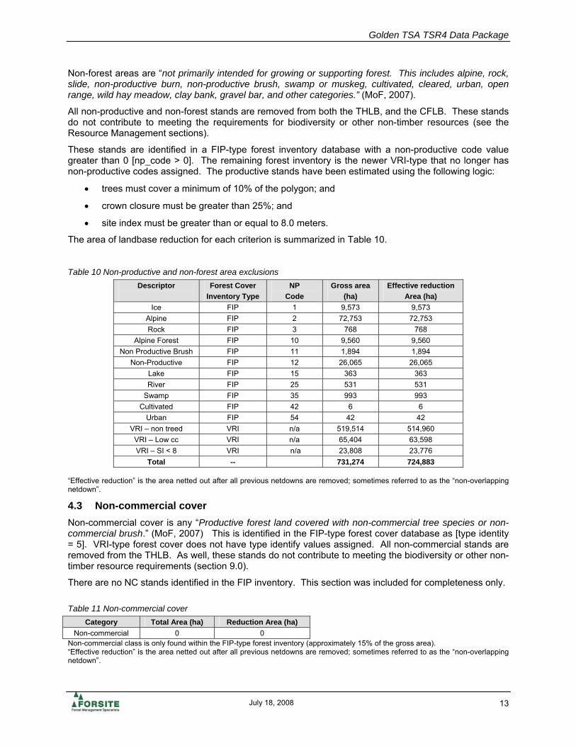
Golden TSA TSR4 Data Package
July 18, 2008 13
Non-forest areas are “not primarily intended for growing or supporting forest. This includes alpine, rock, slide, non-productive burn, non-productive brush, swamp or muskeg, cultivated, cleared, urban, open range, wild hay meadow, clay bank, gravel bar, and other categories.” (MoF, 2007).
All non-productive and non-forest stands are removed from both the THLB, and the CFLB. These stands do not contribute to meeting the requirements for biodiversity or other non-timber resources (see the Resource Management sections).
These stands are identified in a FIP-type forest inventory database with a non-productive code value greater than 0 [np_code > 0]. The remaining forest inventory is the newer VRI-type that no longer has non-productive codes assigned. The productive stands have been estimated using the following logic:
• trees must cover a minimum of 10% of the polygon; and
• crown closure must be greater than 25%; and
• site index must be greater than or equal to 8.0 meters.
The area of landbase reduction for each criterion is summarized in Table 10.
Table 10 Non-productive and non-forest area exclusions
Descriptor
Forest Cover Inventory Type
NP Code
Gross area (ha)
Effective reduction Area (ha)
Ice FIP 1 9,573 9,573 Alpine FIP 2 72,753 72,753 Rock FIP 3 768 768
Alpine Forest FIP 10 9,560 9,560 Non Productive Brush FIP 11 1,894 1,894
Non-Productive FIP 12 26,065 26,065 Lake FIP 15 363 363 River FIP 25 531 531
Swamp FIP 35 993 993 Cultivated FIP 42 6 6
Urban FIP 54 42 42 VRI – non treed VRI n/a 519,514 514,960
VRI – Low cc VRI n/a 65,404 63,598 VRI – SI < 8 VRI n/a 23,808 23,776
Total -- 731,274 724,883 “Effective reduction” is the area netted out after all previous netdowns are removed; sometimes referred to as the “non-overlapping netdown”.
4.3 Non-commercial cover Non-commercial cover is any “Productive forest land covered with non-commercial tree species or non-commercial brush.” (MoF, 2007) This is identified in the FIP-type forest cover database as [type identity = 5]. VRI-type forest cover does not have type identify values assigned. All non-commercial stands are removed from the THLB. As well, these stands do not contribute to meeting the biodiversity or other non-timber resource requirements (section 9.0).
There are no NC stands identified in the FIP inventory. This section was included for completeness only. Table 11 Non-commercial cover
Category Total Area (ha) Reduction Area (ha) Non-commercial 0 0
Non-commercial class is only found within the FIP-type forest inventory (approximately 15% of the gross area). “Effective reduction” is the area netted out after all previous netdowns are removed; sometimes referred to as the “non-overlapping netdown”.

Golden TSA TSR4 Data Package
July 18, 2008 14
4.4 Roads trails and landings A small proportion of the roads may be large enough to be typed as non-forest polygons on the forest cover map. However, these classified roads, trails and landings are not identified as roads per se; they are usually lumped with other non-forest types such as “urban”. Classified roads, trails and landings are, therefore, a portion of the non-forest reductions in Table 8.
4.5 Unclassified roads, trails and landings Most of the roads, trails and landings (RTL) are too narrow to be typed out as polygons in the forest inventory map. These roads are referred to as unclassified. The landbase reduction for unclassified roads was performed by determining an average disturbance width for three classes of roads: 28 m (14 m. each side of centerline) for paved roads, 0 m for trails, and 14 m (7 m. each side of centerline) for all other non-paved and non-trail road type, and then buffering the roads in the GIS. The buffers then were used as landbase netdowns, as per Table 12.
These three road classes correspond to the three classes used in TSR3. However, in TSR3 the analysts assumed that paved roads likely fell on non-forest polygons in the forest inventory, and so no accounting for paved roads was done in TSR3. The road database used in this analysis contained few roads classified as paved, most of these were municipal roads within the city of Golden, so the vast majority of roads in this analysis are “other roads” (Table 12). Table 12 Reductions for unclassified roads, trails, and landings
(1) Road Type
(2) Road Width
(m)
(3) Reduction
(%)
Road Length
(km)
Gross area (ha)
Effective reduction area (ha)
Paved roads 28 100 Other roads 14 100
4915 6,314 4,076
Trails 0 0 1315 0 0
Totals - 6230 6,314 4,076 Width is total buffer width, e.g. 14m represents 7m on each side of the road centreline. “Effective reduction” is the area netted out after all previous netdowns are removed; sometimes referred to as the “non-overlapping netdown”.
The landbase reduction for future roads, trails and landings is described in section 4.16.2.
4.6 Parks and Protected Areas The reduction area of parks and protected areas is summarized in Table 13. Table 13 Reductions for parks and protected areas
Classification Productive Forest Area (ha) Effective Reduction Area (ha) Parks and Protected 290,917 88,227
“Effective reduction” is the area netted out after all previous netdowns are removed; sometimes referred to as the “non-overlapping netdown”.

Golden TSA TSR4 Data Package
July 18, 2008 15
4.7 Inoperable / Inaccessible Area that is not available for timber harvesting due to physical, silvicultural or regeneration difficulties, and economic inaccessibility is classified as “inoperable”. Three classes exist in the operability inventory: inoperable, denoted as “I” (Inoperable) or “N” (non-classified, within Parks) and operable (denoted as “A”). The area of classes “I” and “N” are treated as landbase reductions, as per Table 14. Table 14 Inoperable land base reduction
Classification Productive Forest Area (ha) Effective Reduction Area (ha) I, N 960,242 165,829
“Effective reduction” is the area netted out after all previous netdowns are removed; sometimes referred to as the “non-overlapping netdown”.
4.8 Unstable terrain and environmentally sensitive areas Environmentally Sensitive Areas (ESA’s) are a broad classification of areas that indicate sensitivity for unstable soils (E1s), forest regeneration problems (E1p), snow avalanche risk (E1a), and high water values (E1h). The ESA classification was originally part of the forest cover inventory. The ESA polygons were copied from the forest cover to a separate map, and the map is essentially unchanged from the original forest cover data.
Where completed the ESA soils mapping has been replaced with Terrain Stability mapping. The new terrain mapping was available for 97.1% of the CFLB, the ESA mapping was used on the remaining 2.9%. This terrain mapping is a composite of several projects, all of which utilized the RIC standards of that time (circa 1990’s). Terrain stability mapping is thought to provide a better estimate of unstable soils than the Es1 mapping, and is used in this analysis for the bulk of the unstable landbase netdown. Where not available, the ESA cover is used to identify landbase netdowns (Table 15).
The landbase reduction for unstable terrain was based on the profile of unstable (class U) and potentially unstable (class P) in the harvest. Analyses were made of the percentage of U and P class terrain classes within the harvest profile of three periods: the last 30 years (for most of the TSA), and for the last 10 years and 5 years. These latter two were for a smaller portion of the TSA. They also excluded blocks that addressed MPB attack as those blocks usually fell on gentler terrain, and including them would bias the results. The analyses showed an increase in the percentage of U and P in the harvest over time, as we approach the present day. The results from the last 10 years were chosen to determine the netdown for unstable terrain. The following procedure was used:
• The profile of unstable (U) and potentially unstable (P) terrain classes within the operable, productive forest landbase was calculated as 5.3% and 18.5%, respectively;
• The harvest profile of U and P terrain classes within the last 10 years harvest is 3.6 and 32%, respectively;
• The harvest profile for the P class shows no avoidance of that class, so no reduction for P class terrain is required, nor applied;
• The harvest profile for the U class shows that 1.7% of the U is being avoided (a raw percentage which is calculated as 5.3 – 3.6 = 1.7). This represents 32% of the U profile (this is a percent of percent, i.e. 32% = 1.7% avoidance of U in the harvest profile / 5.3% of U in the landbase profile.)
• If the trend from this last 10 years continues, then we expect 32% of the U class polygons will not have been harvested after the whole THLB is developed. And, 32% is our best estimate of the landbase netdown for U class terrain.
• Using an equivalent area concept, 32% of the U class polygons were randomly chosen, and these polygons were treated as a landbase netdown.
The resulting landbase netdowns for unstable terrain and ESAs (where terrain mapping did not exist) are summarized in Table 15.

Golden TSA TSR4 Data Package
July 18, 2008 16
Table 15 Unstable terrain and environmentally sensitive sites
Description Percentage Removal Productive Forest Area (ha) Effective Reduction (ha) ESA Soils S1 90 612 381 ESA Soils S2 10 6 6
Unstable terrain TSIL U 32 27,743 2,988 Total 28,360 3,376
ESA percentage removals are from TSR 3. The ESA classes in TSR3 included other types of ESA, such as avalanche-type ESAs but those types were not found within the area not covered by the new terrain mapping. 32%% of the unstable areas were removed, roughly consistent with field practices. “Effective reduction” is the area netted out after all previous netdowns are removed; sometimes referred to as the “non-overlapping netdown”. By far, the majority of the unstable terrain class U polygons fall within the inoperable, so the effective reduction area is only a small portion of the total area of class U polygons.
4.9 Non-merchantable / low site and Problem Forest Types Non-merchantable forest types are stands that contain tree species not currently utilized, or timber of low quality, small size and/or low volume, or steep topography, or low stocking.
4.9.1 Non-merchantable / low site
Site class is “The measure of the relative productive capacity of a site for a particular crop or stand, generally based on tree height at a given age” (MoF 2007). Low site stands grow so slowly that they are not deemed to be suitable for forest production. The landbase reductions for low site stands are summarized in Table 16. Table 16 Landbase reductions for non-merchantable, low site types
Class Leading Species
Inventory Type
Groups
Site index Or volume
(m^3)
Age (years)
Productive area
reduction (ha)
Effective area
reduction (ha)
Low Productivity Site Index1
Spruce, Hemlock, Balsam
12-26
<= 8.0
Any 89,185 1,048
Low Productivity Site Index1
Fir, Cedar, Pw, Pl, Py,
Larch, Decid
1-11, 27-42
≤ 9.0 Any 549,968 2,020
Total
639,154 3,067
1 Not applied where stands have logging history and are within the operable. “Effective reduction” is the area netted out after all previous netdowns are removed; this is sometimes referred to as the “non-overlapping netdown”.
Table 17 provides estimates of the stand diameter and volumes at the upper limits of the low site classes. Note that Table 16 is a cut-off value for including/excluding stands in the THLB, and Table 17 is the volume and diameter expected at the same site index values at a reference age=100. If one varies the reference age then one can derive the same numbers as seen in Table 16. And, if the threshold values in Table 16 were varied then the minimum merchantability criteria will force changes in the minimum harvest ages.

Golden TSA TSR4 Data Package
July 18, 2008 17
Table 17 Non-merchantable forest types –diameter and volumes at threshold site index Leading Species
SI Upper Limit
Diameter (cm) at breast Height (cm)
at upper limit of low site
Volume/ha at
upper limit of Low site (m3/ha)Pine ≤ 9.0 17.4 94.4 Fir ≤ 9.0 23.1 17.3
Cedar ≤ 9.0 20.3 72.8
Spruce ≤ 8.0 21.2 44.8 Hemlock ≤ 8.0 22.8 56.0 Balsam ≤ 8.0 21.4 63.7
Notes: Upper limit d.b.h. and volume are based on a reference age of 100 years; FIZ G, and PSYU 175.
4.9.2 Problem Forest Types
In the Golden TSA the deciduous-leading (hardwood) stands are not considered economically viable. These and the older, high percentage hemlock stands were excluded from the timber harvesting land base (Table 18). Table 18 Problem Forest Types
Class Leading Species
or Criteria
Inventory Type
Groups
Site index Or volume
(m^3)
Age (years)
Productive area
reduction (ha)
Effective area
reduction (ha)
Deciduous1 Any deciduous 35-42 n/a > 30 yr 15,929 4,787 Hemlock Hw ( >= 80%) 12-17 n/a 141 + 4,247 761
Total 20,176 5,548 1 Natural stands only, not applied to operable stands with a logging history. “Effective reduction” is the area netted out after all previous netdowns are removed; this is sometimes referred to as the “non-overlapping netdown”.
4.10 Wildlife: Caribou habitat 4.10.1 HLPO caribou habitat requirements
When the OGMAs were being mapped, the equivalent area of the HLPO requirements for caribou were also mapped. Where possible, areas were identified that met both objectives. Caribou areas are also managed as “no harvest” zones, and are therefore treated as landbase exclusions in this analysis. This contrasts with the previous timber supply review where the caribou requirements were modelled as percentage older forest requirements.
4.10.2 SARCO caribou habitat requirements
The Species At Risk Coordination Office (SARCO) recently identified caribou habitat areas that are additional to the HLPO caribou requirements. The SARCO area are also expected to be managed as “no harvest” zones, and therefore are modelled as landbase exclusions in this analysis. The area of HLPO and SARCO caribou habitat exclusions are summarized in Table 19.

Golden TSA TSR4 Data Package
July 18, 2008 18
Table 19 Caribou habitat landbase exclusions
Source of Caribou Habitat Mapping
Productive area (ha)
Effective reduction area (ha)
Caribou - HLPO Mature 20,426 6,157 Caribou - HLPO Old 2,595 1,834 Caribou - SARCO 507 356
Wildlife (Caribou) Total 23,529 8,348
“Effective reduction” is the area netted out after all previous netdowns are removed; sometimes referred to as the “non-overlapping netdown”.
4.11 Cultural heritage and Archaeological reductions Archaelogical Overview (AOA) mapping has been completed for all of the TSA. As development proceeds, detailed archaeological impact assessments (AIA) are completed. To date, the area reserved from forestry activities for protection of heritage resources at the site-specific level has been very small. The area reduction does not significantly impact the timber supply analysis.
Maps of the registered archaeological and heritage sites were obtained from Archaeology Branch. There are 121 individual sites, most being very small, some only 1 square meter. Only those sites over 0.02 ha were incorporated into the data as the very small polygons would have simply been removed by the GIS during the sliver removal process. The gross area of archaeological sites was 14.3 ha (number of sites=55), with a final, effective reduction area of 0.09 ha (Table 20). Table 20 Registered archaeological site reductions Archaeological
Sites (#) Productive Area (ha) Effective Reduction Area (ha)
55 13.82 0.09 “Effective reduction” is the area netted out after all previous netdowns are removed; sometimes referred to as the “non-overlapping netdown”.
4.12 Riparian reserves and management zones – streams Riparian reserve strategies were implemented in the model by establishing effective reserve buffers around the riparian features inventories (streams, wetlands, lakes) using a GIS.
The HLPO specifies a 30 meter reserve around streams for a specified distance upstream of water intakes (also called points of diversion, or POD). The distance upstream is based on stream order. PODs were located, and the streams with reserves were mapped by hand, and GIS buffers created. The riparian exclusions for HLPO-type stream reserves are summarized in Table 21.

Golden TSA TSR4 Data Package
July 18, 2008 19
The remainder of the riparian reductions were based on Forest and Range Practices Regulation (FRPR) defaults. To implement this as a landbase net-down, an effective reserve width is determined by adding the effective retention width for the default management zone width to the reserve buffer and assuming it is a (100%) reserve-type buffer (Table 21). Table 21 Riparian reserve zones – streams
Riparian Class
Riparian Reserve
Zone (metres)
Riparian management
Zone (metres)
Retention Level
(% basal area)
Effective Reserve Width
(metres)
Productive area (ha)
Effective area
reduction (ha)
DWS Stream Reserves 30 0 100 30 451 92 S1a 0 100 20 20 4,798 279 S1b 50 20 20 54 10,187 2,003 S2 30 20 20 34 6,330 1,260 S3 20 20 20 24 4,015 776 S4 0 30 10 3 1,776 324 S5 0 30 10 3 754 63
Total 28,312 4,798 Notes: Based on FRPR Sec 47 to 51. “Effective reduction” is the area netted out after all previous netdowns are removed; sometimes referred to as the “non-overlapping netdown”.
4.13 Riparian reserves and management zones – wetlands and lakes The reserves and management zones for wetlands and lakes were handled the same way as the streams (above). Effective width landbase reductions are listed in Table 22 and Table 23. Table 22 Riparian reserve zones –lakes
Riparian Class*
Riparian Reserve
Zone (metres)
Riparian Management
Zone (metres)
Retention Level
(% basal area)
Effective Reserve Width
(metres)
Productive area
(ha)
Effective area
reduction (ha)
Rip L1b 10 0 10 10 2,917 28 Rip L3 0 30 10 3 698 3
Rip Lake total 3,615 31 Notes: Based on FRPR Sec 47 to 51 * The table only includes the lake classes that occur in the TSA and require riparian reserves (e.g. class L1A do not). “Effective reduction” is the area netted out after all previous netdowns are removed; sometimes referred to as the “non-overlapping netdown”.
Table 23 Riparian reserve zones - wetlands
Riparian Class*
Riparian Reserve
Zone (metres)
Riparian Management
Zone (metres)
Retention Level
(% basal area)
Effective Reserve Width
(metres)
Productive area
(ha)
Effective area
reduction (ha)
W1 10 40 10 14 4,450 290 W3 0 30 10 3 866 75
Total 5,316 365 Notes: Based on FRPR Sec 47 to 51 * The table only includes the wetland classes that occur in the TSA. “Effective reduction” is the area netted out after all previous netdowns are removed; sometimes referred to as the “non-overlapping netdown”.

Golden TSA TSR4 Data Package
July 18, 2008 20
4.14 Biodiversity 4.14.1 Biodiversity – Wildlife Tree Retention Areas
Reserves for existing wildlife tree retention and other cutblock-level, mapped reserves are tallied in Table 24. These areas are the mapped WTPs and other reserves. During the modelling runs they will be set to no-harvest status, and treated as non-THLB. Table 24 Wildlife tree retention and block-level reserves
Class Productive area (ha) Effective reduction area (ha) WTP and other reserves 2,600 1,543
“Effective reduction” is the area netted out after all previous netdowns are removed; sometimes referred to as the “non-overlapping netdown”.
4.14.2 Old Seral and Mature-plus-old Seral
The Higher Level Plan Order specifies the percentage requirements of old seral and mature-plus-old seral that must be retained within each LU and BEC combination. The equivalent area of both the old and mature-plus-old seral has been mapped by ILMB staff. These areas are called OGMAs (old growth management areas) and MOGMAs (mature old growth management areas). They are modelled as “no-harvest” zones and are treated as landbase exclusions in this analysis. In TSR 3 the biodiversity requirements were modeled as percentage older seral requirements. The exclusions of each type are summarized in Table 25. Table 25 OGMA and MOGMA landbase exclusions
Biodiversity Reserve Type
Productive area (ha)
Effective reduction area (ha)
Old growth management area (OGMA) 11,074 720 Mature plus old management area (MOGMA) 44,416 9,190
Totals 55,490 9,910 “Effective reduction” is the area netted out after all previous netdowns are removed; sometimes referred to as the “non-overlapping netdown”.
4.15 Permanent sample plots The landbase reductions for reserves around permanent sample plots (PSP) are provided in Table 26. Table 26 Permanent sample plot reductions
PSP Reserves Productive Area (ha) Effective Reduction Area (ha) Total 190 105
“Effective reduction” is the area netted out after all previous netdowns are removed; sometimes referred to as the “non-overlapping netdown”.

Golden TSA TSR4 Data Package
July 18, 2008 21
4.16 Future Land Base Reductions 4.16.1 Future wildlife tree retention areas
The licensees’ Forest Stewardship Plans are based on retaining the default 7% of each cutblock as wildlife tree retention areas (WTRA). When possible, WTRAs are placed within existing non-THLB stands, so only a portion of the 7% is actually a landbase reduction. Wildlife tree retention areas are required to be placed at a maximum distance of 500 meters apart. Based on these two factors (7.0% of the THLB reserved when beyond the 500m maximum distance spacing) the area of future wildlife tree retention areas (Table 27) was estimated using the following procedure. • Within the THLB (Table 27, column 1) apply a 500m buffer around all productive, non-THLB stands to
determine the THLB area within 500 m of existing stands that could meet WTRA requirements(column 2); • The area outside the buffer is the area that requires additional wildlife tree retention (column 3); • Apply a 7% retention rate to this area to estimate the equivalent area of future wildlife tree retention
(column 4); • Calculate the equivalent, blended rate of retention across the whole THLB (the developed area plus the
un-developed area), which is 0.4604 % of the THLB (column 5); • Apply that percentage as a yield curve reduction against all the future managed stand yield curves. Table 27 Estimate of future wildlife tree retention areas
(1) Sample THLB Area (ha)
(2) THLB Area within
500 meters of NHLB
(%)
(3) THLB Area
requiring additional WT retention
(%)
(4) Equivalent THLB Retention Area
Assuming 7% Retention (7%) X (3)
(ha)
(5) Future THLB
Reduction (4) / (1)
(%) 141,525 93.422 % 6.578 % 652 ha 0.4604 %
4.16.2 Future roads, trails and landings
A recent Forest Practices Branch audit of licensee blocks found that only 4.6% of the area of cutblocks was in permanent access structures (PAS). This included roads, trails and landings. Based on this factor (4.6% of THLB), the area of future roads, trails and landings (Table 28) was estimated using the following sequence: • Within the THLB (Table 28, column 1) apply a 300m buffer around all existing mapped roads to determine
the “developed area” (column 2); the remaining THLB area is the “undeveloped area”; • Within the undeveloped THLB area (column 3), apply a 4.6 % reduction to find the total area (in hectares)
representing all future roads, trails and landings (column 4); this translates to a blended percentage of the total THLB landbase (column 5); and
• Apply that blended percentage as a reduction to the future, managed stand yield curves (column 5). Table 28 Estimate of future roads, trails, and landings
(1) THLB Area
(ha)
(2) Developed
THLB Area (%)
(3) Non-developed
THLB Area (%)
(4) (4) Equivalent THLB Retention Area
Assuming 4.6% Area in PAS (3) X (4.6%)
(ha)
(5) Future THLB
Reduction (4) / (1)
(%) 141,525 61.365 % 38.635 % 2,516 1.778 %

Golden TSA TSR4 Data Package
July 18, 2008 22
4.17 Area additions No area is added to the landbase during the modelling. In TSR3 there were some Timber Licences that did revert, however the last of the Timber Licenses in the TSA reverted to the Crown just prior to the beginning of this timber supply analysis (March 31, 2008).
4.18 Descriptions of the Landbase The exclusions described previously define the extent of the productive forest land, and the timber harvest landbase. The characteristics of their age class distribution, species profile and site index profile follow.
4.18.1 Age Class distribution
Statistics and charts of the age class distribution are provided in Table 29, and Figure 2 and Figure 3 . Site index for the contributing and timber harvesting land base is depicted in Figure 4. The average site index of the THLB is 17.1 m.
Table 29 Golden TSA Age class distribution
Age Range Productive Total (ha)
Operable (ha)
Timber harvesting Land base (ha)
0 6,263 5,903 5,552 1-20 14,819 14,154 13,287
21-40 46,770 41,803 39,911 41-60 12,903 5,835 4,615 61-80 30,060 13,418 10,767
80-100 48,496 21,503 17,914 101-120 36,487 12,599 10,082 121-140 37,891 10,890 8,409 141-250 127,641 28,294 17,894
251+ 71,347 26,338 13,099 Totals 432,677 180,738 141,530
0
20000
40000
60000
80000
0 50 100 150 200 250
Age
Are
a (h
a)
NCLB THLB

Golden TSA TSR4 Data Package
July 18, 2008 23
Figure 2 Age class distribution of non-contributing (NHLB) and timber harvesting landbase (THLB)

Golden TSA TSR4 Data Package
July 18, 2008 24
Figure 3 Age class distribution by species group for timber harvesting landbase (THLB)
Spruce and Balsam leading stands cover 40% of the THLB area. Other species groups and their percentage are: Fir and larch (25%), Pine (19%), Cedar/Hemlock (13%) and Deciduous (3%).
Figure 4 Site index for non-contributing (NCLB) and timber harvesting landbase (THLB).
0
10,000
20,000
30,000
40,000
50,000
0 1 2 3 4 5 6 7 8 9
Age Class
Are
a (h
a)Decid
FL
CH
SB
Pine
0
10,000
20,000
30,000
40,000
50,000
60,000
70,000
80,000
90,000
2 4 6 8 10 12 14 16 18 20 22 24 26 28 30
Site Class
Are
a (h
a)
NHLB THLB

Golden TSA TSR4 Data Package
July 18, 2008 25
5.0 Inventory Aggregation 5.1 Analysis Units To reduce the complexity and volume of information in the timber supply analysis, individual stands are aggregated into ‘analysis units’ (AU). Groups are largely based on dominant tree species (inventory type group), timber growing capability (site index) and silvicultural management regimes. For example, all fir/larch stands on moderate growing sites with a clearcut silviculture regime may be grouped into a single analysis unit. Each analysis unit has at least one associated yield table that provides the model with the net merchantable volume that is available for harvest at different stand ages.
Several sets of analysis units were created to reflect forest management practices on the THLB:
Existing non-harvested, natural stands (100 series – 95,727 ha of THLB)
These are stands with no history of harvesting in the past. Most of these stands are >=30 years old today but some younger stand created through natural disturbances are also included. Once harvested, these stands move onto the 200 series as future managed stands (clearcut).
Future managed stands (200 series – same area as 100 series)
These analysis units are the same as the 100 series analysis units after being harvested. The 200 and 600 series analysis units (see below) undergo the full benefits of forest management practices, such as better initial stocking and planting of stock with higher genetic gains.
Existing clearcut, managed stands (500 series – 45,803 ha of THLB)
These are previously logged stands. Forest management has had some positive impact on the establishment and growth of these stand compared to natural stands, but not as much as stands logged from today forward. Most of these stands are less than 30 years old today. Once harvested, these stands move onto the 600 series and realize the full benefits of current regeneration practices, such as volume gains from the use of select seed.
Future existing-managed stands (600 series – same area as 500 series)
These analysis units are the 500 series analysis units after being harvested.
Non-contributing stands (800 series – 0 ha of THLB; 291,147 ha of NHLB)
These are productive stands in the non-timber harvest land base (NHLB). They track along their own yield curve, undergo disturbances, but do not experience any harvesting. They contribute to biodiversity and other resource requirements.
These broad groups are further sub-divided by criteria of: • leading species, and • NSR class (not sufficiently restocked), and • site index (to differentiate the regeneration and growth characteristics). Classification thresholds for defining analysis units were determined by balancing the competing objectives of using the fewest number of analysis units (to reduce unnecessary complexity), that are significantly different (in terms of biology, growth characteristics, etc), while trying to maintain reasonable-sized areas (hectares) of each analysis unit. The common species and site index thresholds chosen for the clearcut-based analysis units are listed in Table 30.
Table 30 Existing stand analysis unit species and site index classification thresholds

Golden TSA TSR4 Data Package
July 18, 2008 26
Leading Species
Logging History
Site Group
Site Index Break- points
Analysis Unit
Inventory Type Groups Name (number)
Douglas-fir, Larch (dry)
NO 1 2 3
>=22 >=17 and <22
<17
Natural - 101 Natural - 102 Natural - 103
F, FPl, FPy, FL, FDecid, LF, L
(1, 5, 6, 7, 8, 33, 34) Douglas-fir
(wet) NO 1
2 3
>=21 >=17 and <21
<17
Natural - 104 Natural - 105 Natural - 106
FC, FH, FS (2, 3, 4)
Cedar NO 1 2 3
>=19 >=14 and <19
<14
Natural - 107 Natural - 108 Natural - 109
C, CF, CH (9, 10,11)
Hemlock NO 1 2 3
>=18 >=13 and <18
<13
Natural - 110 Natural - 111 Natural - 112
H, HF, HC, HB, HS, HDecid (12, 13, 14, 15, 16, 17)
Balsam, Spruce S predominant
NO 1 2 3
>=18 >=13 and <18
<13
Natural - 113 Natural - 114 Natural - 115
B, BH, BS, S, SB (18, 19, 20, 21, 24)
Spruce mixed
NO 1 2 3
>=21 >=17 and < 21
<17
Natural - 116 Natural - 117 Natural - 118
SF, SH, SPl, SDecid (22, 23, 25, 26)
Pine NO 1 2 3 4
>=21 >=19 and <21 >=16 and <19
<16
Natural - 119 Natural - 120 Natural – 121 Natural - 122
PwPa, Pl, PlF, PlS, PlDecid, Py (27, 28, 29, 30, 31, 32)
Decid YES (1) Any Any Natural – 123 CotConif, CotDecid, DConif, DDecid, Mb, Bi, AConif, ADecid (35, 36, 37, 38, 39, 40, 41, 42)
Douglas-fir, Larch (dry)
YES (2) Any ALL Existing Managed – 501
F, FPl, FPy, FL, FDecid, LF, L
(1, 5, 6, 7, 8, 33, 34) Douglas-fir
(wet) YES (2) Any ALL Existing
Managed – 502 FC, FH, FS
(2, 3, 4) Cedar YES (2) Any ALL Existing
Managed – 503 C, CF, CH (9, 10,11)
Hemlock YES (2) Any ALL Existing Managed – 504
H, HF, HC, HB, HS, HDecid (12, 13, 14, 15, 16, 17)
Balsam, Spruce S predominant
YES (2) Any ALL Existing Managed – 505
B, BH, BS, S, SB (18, 19, 20, 21, 24)
Spruce mixed
YES (2) Any ALL Existing Managed – 506
SF, SH, SPl, SDecid (22, 23, 25, 26)
Pine YES (2) Any ALL Existing Managed – 507
PwPa, Pl, PlF, PlS, PlDecid, Py (27, 28, 29, 30, 31, 32)
Deciduous (logged)
YES (2) Any ALL Existing Managed – 508
CotConif, CotDecid, DConif, DDecid, Mb, Bi, AConif, ADecid (35, 36, 37, 38, 39, 40, 41, 42)
Backlog 1 (fire or logged)
YES (3) Any ALL, >= 60% MSS (4)
Existing Managed – 525
(3)
Backlog 2 (fire or logged)
YES (3) Any ALL, < 60% MSS (4)
Existing Managed - 526
(3)
Notes: YES (1) = With any history of logging; YES (2) = History of logging within last 30 years; YES (3) = History of logging or wildfire (3) = Any leading species, the areas are statistically assigned based on silviculture records. (4) = Backlog NSR areas are is divided into those above and below 60% Minimum Stocking Standards (MSS)

Golden TSA TSR4 Data Package
July 18, 2008 27
6.0 Growth and Yield This section describes the information/data sources, assumptions, and methods for generating growth and yield estimates for the analysis units described in section 5.1.
6.1 Site Index Site index (SI) is a measure of the stand's productive potential for a particular tree species. SI in British Columbia is expressed as potential tree height at 50 years breast height age. SI provides standardized comparisons of productive potential between sites, across a broad range of existing stand conditions. As such, we use it as a silvicultural tool to prescribe treatments and analyze investments. SI also serves as the main driver for many growth and yield models, which predict future forest growth and timber yields. Reference: SiteTools V3.3
6.1.1 Site curves
The standard, MoF site index curves are utilized throughout this analysis. Table 31 Standard MoF site index curves
Species Source Douglas Fir (Fdi) + (Pw, Py) Thrower and Goudie (1992)
Western Larch (Lw) Brisco, Klinka, and Nigh 2002 Lodgepole Pine (Pli) Thrower (1994)
Western Red Cedar (Cwi) Nigh (2000) Western Hemlock (Hwi) Nigh (1998)
White Spruce (Sw) + (Sx) Nigh (1997) Englemann Spruce (Se) Chen and Klinka (2000)
Balsam fir (Bl) Chen and Klinka (2000) Trembling Aspen (At) Nigh, Krestov and Klinka (2002)
6.1.2 Site index adjustments
No site index adjustments were used in this analysis.
6.2 Utilization level Utilization levels define the maximum height of stumps that may be left on harvested areas, the minimum top diameter (inside bark), and the minimum diameter at breast height (dbh) of stems that must be removed from harvested areas. These factors (Table 32) are used when calculating the merchantable stand volume in the analysis. Table 32 Utilization levels
Utilization Species Minimum dbh Maximum stump height Minimum top dib
Pl 12.5 30 10 All others 17.5 30 10
Notes: dbh = diameter at breast height. Dib = diameter inside bark; Deciduous species and Pa are netted out of stand volumes
6.3 Decay, waste and breakage for natural stands Decay, waste and breakage factors are applied to natural stand yield tables to obtain net harvest volumes per hectare. This analysis used the standard values incorporated into the Variable Density Yield Prediction (VDYP 6) model, which are based on species, age, and Special Cruise Number (SC, or PSYU number.)

Golden TSA TSR4 Data Package
July 18, 2008 28
6.4 Operational adjustment factors for managed stands 6.4.1 Standard Operational Adjustment Factors
Operational Adjustment Factors (OAFs) were applied to adjust (reduce) the yields generated by the TIPSY growth and yield model down to net operational volumes. This included reductions for such factors as gaps in stand stocking, decay/waste/breakage, and endemic forest health losses.
Two types of OAFs were used in the TIPSY model. OAF 1 is a constant percentage reduction to account for openings in stands, distribution of stems or clumping, endemic pests and diseases, and other risks to potential yield. OAF 2 is an increasing percentage reduction that can be applied to account for decay, waste and breakage. OAF 2 is applied after OAF 1 and increases linearly over time from 0 percent at age 0 to the specified percentage at 100 years of age. The OAF1 and OAF2 value used in this analysis were the provincial defaults of 15% and 5%, respectively.
6.5 Volume reductions All deciduous stands are netted out of the THLB, except for stands with a previous history of logging, and the deciduous component is netted out of coniferous leading stand yield curves (Table 33). Similarly, all whitebark pine (Pa) leading stands or components of other stands are removed from the THLB or yield curves, respectively. Table 33 Volume reductions
Stand type Definition Volume reduction Deciduous ITG = 35 to 42 100%
Pa ITG = 28 to 31 Pa leading stands removed 100% from the THLB. Deciduous component of coniferous leading stands
Other ITGs 100% of the deciduous volume; 0% of coniferous volume
Note: ITG = Inventory Type Group
6.6 Yield table development – Natural Stands Stands are grouped into analysis units primarily based on similar species and site index value. A yield table is developed for each analysis unit.
6.6.1 Methodology
Natural stand yield table values were based on weighting the yield curves for each forest stand. These were derived using VDYP 6 software. The sequence of developing the yield curves was: • Project all stands to 2008 (end of growing season 2007); • For those polygons that were adjusted the adjusted age and adjusted height were used to estimate a new
site index; • The species and (adjusted) site index were used to assign each stand to an analysis unit (AU), and/or the
species, site index and volume were used to assign the stand to a netdown type. • After netdowns and AU assignment, an AU yield curve was calculated by area-weighting the volume
estimates at each time step (i.e. at time = 10 years, 20 years, etc) from each of the stand yield curves. • Percentage reductions were applied to future managed stand yield curves for future wildlife tree patches
and future RTLs. They were not applied to the natural stand yield curves. Natural stand analysis unit yield curves are included as Appendix A. The site index values for the clearcut analysis units are in Table 34. The site index values for the NCLB analysis units are in Table 35.

Golden TSA TSR4 Data Package
July 18, 2008 29
Table 34 Site index assignments for THLB natural stand analysis units.
Analysis Unit
Leading Species
Site Group
Area (ha)
Natural stand site Index
Regenerates To AU #
3,201 23.7 12,347 18.0
101 102 103
Fd (Dry) and Lw
1 2 3 0 n/a
201 202 203
2,268 23.4 7,067 18.6
104 105 106
Fd (wet) 1 2 3 4,357 15.5
204 205 206
877 19.1 3,897 15.6
107 108 109
Cw 1 2 3 1,169 12.9
207 208 209
792 18.8 2,309 14.7
110 111 112
Hw 1 2 3 3,385 11.2
210 211 212
3,650 20.8 8,389 15.1
113 114 115
B, S predominant 1 2 3 5,112 11.0
213 214 215
3,260 23.4 4,634 18.9
116 117 118
S mixed
1 2 3 7,642 13.9
216 217 218
3,754 22.5 3,652 19.9 9,944 17.1
119 120 121 122
Pine 1 2 3 4 2,704 14.7
219 220 221 222
123 Decid All 1,317 21.1 223
Notes: AU 123 = Operable stands, with a history of logging over 30 years ago, without no additional genetic worth (versus those that were harvested within last 30 years and are assigned to the existing managed AUs) that have regenerated back to deciduous leading but should not be netted out of the THLB landbase. Table 35 Site index assignments for non-THLB (NHLB) contributing analysis units
AU
Notes Leading Species
Site Group
Area (ha)
Site Index
Regenerates To AU #
801 NHLB Conif Coniferous All 282,068 14.2 801 802 NHLB Decid Deciduous All 9,084 19.2 802
6.6.2 Existing timber volume check
The total forest volume was estimated based on the yield curves, and compared to the volume estimated in the forest inventory (VDYP projected volumes, after adjustments for age, height, and volume). Table 36 is a comparison of the two estimates. The volumes are net of the deciduous-leading stands, and net of the deciduous and Pa component volumes. Table 36 Timber Volume Check
Stand Type Inventory Polygon volume ( m3)
Yield table (AU) volume ( m3)
Percent (%) Difference
THLB Natural 26,828,028 26,405,823 1.6 NHLB 80,381,400 80,315,438 0.1

Golden TSA TSR4 Data Package
July 18, 2008 30
6.7 Yield table development - managed stands This section summarizes the inputs used in the TIPSY growth and yield model for the managed stand analysis units (200 and 600 number series). Natural stands (100 series) move onto matching 200 series analysis units after harvest. When existing managed stands (500 series) are harvested, they move onto the future managed stand AU’s (600 series). These are identical to the 500 series but reflect the genetic gains for future managed stands.
6.7.1 Silviculture management regimes
Only clearcut systems were modelled in this analysis. A small portion of the stands in the TSA are partial cut, but the small area did not warrant creating separate partial-cut type analysis units.
Average, historical regeneration practices were reflected in the existing managed stand AU inputs (500 series AUs) while current regeneration practices are reflected in the future managed stand AU inputs (200 and 600 series). 6.7.2 Regeneration delay
Regeneration delay is the time between harvesting and the time when a new stand is initiated. The delay incorporates both the time taken to establish a stand, and the age of seedling stock planted, if applicable. For this analysis, a regeneration delay was estimated based on local knowledge of the licensees’ silviculture staff.
Existing managed stands.
For existing managed stands, regeneration delay was addressed through the use of actual stand age in the forest inventory file. This age represents the actual age of the stand and not the time since harvesting. For example, a stand may have been harvested 15 years ago but the current stand age is 12 – this implies a 3 year regeneration delay. The use of actual ages eliminated the need to estimate an average regeneration delay for these stands.
Future managed Stands
A regeneration delay of 2 years was estimated based on the local knowledge of the licensees’ silviculture staff. Regeneration delays for future managed stands were input into TISPY and are therefore embedded in the published yield curves.
6.7.3 Stand rehabilitation
There is no active program of stand rehabilitation in the TSA. No rehabilitation of problem forest or non-merchantable types was included in the model.
6.7.4 Genetic improvement
As required by the Chief Forester’s Standards for Seed Use (Nov 23, 2006), the licensees use select seed for regeneration purposes when reasonable gains are projected. This section describes the yield adjustments used in this analysis to account for the use of select seed (i.e., orchard & select provenance seed with a known genetic gain as measured by Genetic Worth [GW]).
The statistics on the historical use of select seed for all the tables in this section was obtained from the Ministry of Forests Seed Planning & Registry system (SPAR), as summarized by L. McAuley (2008) and B. Wadey (2008). This information was used to derive current practice estimates of net genetic gain (Net GW) at the species level (Table 37). This table illustrates the weighted average GW for each species for the last 5 years [A], the percent improved (class A and B) seed use for each species in the TSA [B], and the estimated Net GW for each species [C]. The Net GW was calculated by multiplying [A] x [B].

Golden TSA TSR4 Data Package
July 18, 2008 31
Table 37 Average net genetic worth of species planted during last 30 years. Wt Avg GW by Species
(Class A) [A] % Class A of Total
Seedlings Planted [B] Net GW by Species
[C] Year
Lw Pw Sx Pli Lw Pw Sx Pli Lw Pw Sx Pli 2003 11 0 18 3 100 100 70 73 11.0 0.0 12.6 2.2
2004 11 0 22 3 75 0 72 60 8.3 0.0 15.8 1.8
2005 11 0 20 3 100 0 94 73 11.0 0.0 18.8 2.2
2006 17 0 24 3 100 0 100 89 17.0 0.0 24.0 2.7
2007 0 0 19 3 77 0 90 0 0.0 0.0 17.1 0.0
5 yr Avg 10.0 0.0 20.6 3.0 90.4 20.0 85.2 59.0 9.5 0.0 17.7 1.8
30 Yr Avg 1.7 0.0 3.4 0.5 15.1 3.3 14.2 9.8 1.6 0.0 2.9 0.3
The 30 years average gains shown are suitable for use in generating existing managed stands yields as they reflect a watered down gain associated with 25 years of planting seed with no gains followed by 5 years of planting with gains . Genetic gains of 1.6% would be applied to Lw, 2.9% to Sx and 0.3% for Pl within the existing managed stands. While class A Pw seedlings have been used in the last 5 years, there is no reported genetic worth value, so 0% net GW was assumed for Pw.
Seed planning units (SPU’s) geographically delineate the appropriate area of seedling use for stock coming from particular seed orchards. Each SPU also has defined elevation range for seedlings. The select seed SPU’s that occur within the Golden TSA are listed in Table 38.
Table 38 Seed Planning Units in Golden TSA (Class A seed)
Species Class A Seed Planning Zone SPU
Min Elev (m)
Max Elev (m)
Western white pine Kootenay Quesnel (KQ) 15 500 1400 Interior Spruce East Kootenay All (EK) 25 750 1700 Interior Spruce Nelson Mid (NE) 04 1000 1500 Lodgepole Pine East Kootenay Low (EK) 32 800 1500 Western Larch East Kootenay Low (EK) 34 800 1500
Fdi East Kootenay Low (EK) 39 700 1400 Fdi Quesnel Lakes Low (QL) 37 700 1400 Fdi East Kootenay Low (EK) 39 700 1400
Increased gains are projected for these SPU’s within 10 years while the planning horizon for this analysis is > 250 years. One estimate for the planning horizon is used. It is reasonable to use the projected gains across the planning horizon in the base case as this will result in an overestimate for only the first decade and then realistic or conservative estimates for the remaining 24 decades.
The future projected gains are estimated as per Table 39. The estimated, future effective genetic worth for each SPU is provided in column [B] while the availability to meet SPU seed needs is provided in column [C]. The projected GW to be achieved (column D) is the product [B] and [C]. It is assumed that seed from the SPU is eligible for use where that species is planted in the TSA.

Golden TSA TSR4 Data Package
July 18, 2008 32
Table 39 Seed planning units (Class A seed) genetic worth and seed availability
SPU % of Seed Use Eligible
to come from SPU
Min Elev (m)
Max Elev (m)
Projected Future Genetic Worth (in Year)
[B]
Projected Availability
(in Year) [C]
Projected Genetic Worth
Achieved In Future [D]
PW KQ (15) 100 500 1400 0 (*) 100 0 (*)
Sx EK All (25) 95% 750 1700 28% (2017+) 75 % (2025+) Sx NE Mid (04) 5% 1000 1500 16% (2014+) 100% (2008+)
(20.0) + (0.8) = 20.8
PLI EK LOW (32) 100 800 1500 12% (2017+) 100% (2019+) 12 LW EK LOW (34) 100 800 1500 20% (2017+) 100% (2008+) 20
FDI EK LOW (39) 80% 700 1400 25% (2013+) 100% (2016+) FDI QL LOW (37) 5% 700 1400 22% (2017+) 100% (2010+)
(20) + (1.1) = 21.1
Values obtained from “Breeding and orchard production” reports (L. McAuley, MoF, 2008) (*) Although Pw Class A seed is produced the genetic worth is not estimated.
The application of this data by AU in the timber supply model is summarized as Table 40, and is included in the TIPSY inputs tables (Table 42). Table 40 Summary of genetic worth used for modelling with each species Species Existing, Managed Stands
Genetic Worth Future Managed Stands,
Genetic Worth Sx 2.9 20.8 Pli 0.3 12 Lw 1.6 20 Fdi 0.0 21.1
In summary, the 30-year historical average from Table 37 was applied when modeling existing managed stands because this best corresponds with the criteria used to define these stands. When generating the AU yields in TIPSY for these stands, larch will have a 1.6% GW applied, while spruce will have a 2.9% GW applied, and Pl will have 0.3% applied. Future managed stands will have one estimate of the varying future net GW applied, usually chosen at reference year=2017. The Net GW’s will be applied to Fd (21.1%), Lw (20%), Pl (12%), and Sx (20.8%). No change in genetic gains was scheduled during the planning horizon.
Genetic gains (Table 40) will be incorporated into the growth and yield curves through TIPSY model functionality. When a species identified in Table 40 is included in a managed stand AU, its associated Net GW will be input into TIPSY. This Net GW reflects the genetic gain associated with all seedlings of a given species planted in a typical year. Where surrogate species were used in TIPSY, the GW employed is prorated to reflect the relative GW’s of the original species (i.e. Sx used for Bl but Sx GW not applied to Bl proportion). 6.7.5 Planting Density
Values of 2000 sph were assumed for all plantations. These values were derived from a combination of the TSA silviculture records and staff experience. These densities are considered to reflect the number of stems competing to be crop trees and are between the values for well-spaced and total-stocking densities.

Golden TSA TSR4 Data Package
July 18, 2008 33
6.7.6 TIPSY managed stand yield table inputs
Existing and future managed yield curves will be derived using the BatchTIPSY (ver 3.2) software with the following inputs. Table 41 Inputs (to TIPSY) for Existing Managed Stand Yield Curves
Existing Managed Stand AU
Regen -
Plant/ Natural
Species Composition Area (ha)
Site Index
OAF VAF
Regen Delay
Utiliz- ation Level
Initial Density
Select Seed Gains
501 – Fd Dry P 100% Fd 40 Se 25 Pl 30 Lw 5 3,779 17.2 (2) 2 17.5 2,000 (6) 502 – Fd Wet P 100% Fd 40, Se 30 Pl 20 Lw 5 Cw 5 2,477 17.8 (2) 2 17.5 2,000 (6)
503 – Cw P 100% Se 40 Cw 40 Fd 10 Hw 10 4,036 18.1 (2) 2 17.5 2,000 (6) 504 – Hw P 100% Se 40 Cw 40 Fd 10 Hw 10 1,376 16.3 (2) 2 17.5 2,000 (6) 505 – B, S P 100% Se 85 Bl 10 PL5 15,479 16.4 (2) 2 17.5 2,000 (6)
506 – S mixed P 100% Sx 60 Cw 20 Fd 10 Pl 10 7,722 15.5 (2) 2 17.5 2,000 (6) 507 – Pine P 100% Pli 60 Se 20 Fd 20 7,228 16.3 (2) 2 12.5 2,000 (6)
508 – Decid (1) P100% At 50 Sx 35 Pl 10 Fd 5 3,031 19.4 (3) 2 17.5 2,000 (6) 525 Backlog 1 N100 S40 Pli22 Fdi 22 C9 H7 376 16.9 (4) 12 17.5 2,000 n/a 525 Backlog 2 N100 S40 Pli22 Fdi 22 C9 H7 302 18.0 (5) 20 17.5 2,000 n/a
AU 508 = Deciduous leading with a history of logging within the past 30 years.
VAF = volume adjustment factor
(2) OAF1 = 15%, OAF2 = 5%; VAF = 1.00 (no adjustment)
(3) OAF1 = 25%, OAF2 = 5%; VAF = 1.00
(4) OAF1 = 15%, OAF2 = 5%; VAF = 0.90 (10 % reduction)
(5) OAF1 = 15%, OAF2 = 5%; VAF = 0.75 (25 % reduction) (6) Genetic Worth varies by species; Value based on the limited use of improved stock in the past.

Golden TSA TSR4 Data Package
July 18, 2008 34
Table 42 Inputs (to TIPSY) for Future Managed Stand Yield Curves
Leading Species
AU No.
Regen Method
Species Composition
Area (ha)
Site Index
Utiliz- ation Level
Initial Density
Select Seed Gains
3,201 23.7 12,347 18.0
Lw, Fd (dry)
201 202 203
P 100% P 100% P 100%
Fd 40, Pli 40, Se20 Fd 40 Pli 40 Se20
Pli 80 Fd 20
17.5 17.5 17.5
2,000 2,000 2,000
(1) (1) (1)
2,268 23.4 7,066 18.6
Lw, Fd (wet)
204 205 206
P 100% P 100% P 100%
Fd 40 Se 40 Cw 10 Pl 10 Fd 40 Se 40 Cw 10 Pl 10
Fd 50 Pl 40 Se 10 4,358 15.5
17.5 17.5 17.5
2,000 2,000 2,000
(1) (1) (1)
877 19.1 3,873 15.6
Cw 207 208 209
P 100% P 100% P 100%
Se40 Cw40 Fd 10 Pw 5 Hw 5 Se40 Cw40 Fd 10 Pw 5 Hw 5
Se 60 Cw 20 Fd 20 1,169 12.9
17.5 17.5 17.5
2,000 2,000 2,000
(1) (1) (1)
792 18.8 2,309 14.7
Hw 210 211 212
P 100% P 100% P 100%
Se 50 Cw 30 Hw 20 Se 50 Cw 30 Hw 20
Se 50 Cw 25 Fd 15 Hw 5 Pli 5 3,385 11.2
17.5 17.5 17.5
2,000 2,000 2,000
(1) (1) (1)
3,650 20.8 8,388 15.1
B, S 213 214 215
P 100% P 100% P 100%
Sx 80 Pli 10 Bl 10 Sx 80 Pli 10 Bl 10
Se 85, Pli 15 5,130 11.0
17.5 17.5 17.5
2,000 2,000 2,000
(1) (1) (1)
3,260 23.4 4,634 18.9
S mixed 216 217 218
P 100% P 100% P 100%
Se 50 Cw 30 Fdi 10 Hw5 Pw5 Se 50 Cw 30 Fdi 10 Hw5 Pw5 Se 50 Cw 30 Fdi 10 Hw5 Pw5 7,642 13.9
17.5 17.5 17.5
2,000 2,000 2,000
(1) (1) (1)
3,754 22.5 3,652 19.9 9,944 17.1
Pine 219 220 221 222
P 100% P 100% P 100% P 100%
Pli 60, Se 20, Fd 20 Pli 60, Se 20, Fd 20 Pli 60, Se 20, Fd 20 Pli 70, Fd 20, Se 10 2,704 14.7
12.5 12.5 12.5 12.5
2,000 2,000 2,000 2,000
(1) (1) (1) (1)
Decid 223 P 100% Sx 70 Pl20 Fd10 1,317 21.1 17.5 2,000 (1)
Lw, Fd Dry 601 P 100% Fd 40 Se 25 Pl 30 LW 5 3,779 17.2 17.5 2,000 (1) Lw, Fd Wet 602 P 100% Fd 40 Se 35 Cw15 Pw5 Lw5 2,477 17.8 17.5 2,000 (1)
Cw 603 P 100% Se 40 Cw40 Hw10 Fd5 Pw5 4,036 18.1 17.5 2,000 (1) Hw 604 P 100% Se 40 Cw40 Fd10 Hw5 Pw5 1,376 16.3 17.5 2,000 (1) B, S 605 P 100% Se 85, Bl 10 PL5 15,479 16.4 17.5 2,000 (1)
S mixed 606 P 100% Se 55 Cw 25 Fd 10 Hw5 Pw5 7,722 15.5 17.5 2,000 (1) Pine 607 P 100% Pl 55 Se 20 Fd 20 Lw5 7,228 16.3 12.5 2,000 (1)
Decid 608 P100% Sx 70 Pl20 Fd10 3,031 19.4 17.5 2,000 (1) Backlog 1
(3) 625 P100% Se 60 Pl 20 Fd10 Cw10
376 16.9 17.5 2,000 (1)
Backlog 2 (3)
626 P100% Se 60 Pl 20 Fd10 Cw10 302 18.0
17.5 2,000 (1)
Notes: (1) Genetic Worth varies by species; Values are based on future use of improved genetic stock. (2) All AU’s: OAF1 = 15%, OAF2 = 5%; Regen delay = 2 years.
AU 223 = Operable stands, previously harvested more than 30 years ago, that originally regenerated back to decidous leading and after the first harvest will be planted to coniferous leading.

Golden TSA TSR4 Data Package
July 18, 2008 35
7.0 Silviculture 7.1.1 Existing managed stands
Existing managed stands are defined as the operable stands with a record of logging within the last 30 years. The 30-year figure corresponds to the time when more intensive silviculture management started within the TSA.
Both existing and future managed stand yield curves were determined using TIPSY. Inputs for the existing managed stands are in Table 42.
7.1.2 Backlog and current non-stocked area (NSR)
Backlog NSR is any area not yet fully stocked that was denuded prior to 1987 when basic silviculture became the obligation of licensees. Not satisfactorily restocked (NSR) areas were determined using RESULTS data. NSR areas include both old burns and past harvesting. Current NSR (2055.2 ha) and backlog NSR (1281.7 ha) is summarized in Table 43. Table 43 Backlog NSR Area
Leading Species
Current NSR
Estimated backlog NSR >= 60% MSS
Estimated backlog NSR < 60% MSS
Any 2055.2 ha 653.7 ha (51% of backlog) 628 ha (49% of backlog)
Note: MSS = Minimum stocking standard.
Backlog NSR has been assigned to analysis units 525 and 526. Backlog NSR records in the RESULTS data are for portions of opening numbers (a combination of Map + Opening Number) which are often several polygons in the forest cover data. Hence, one cannot identify the forest cover polygons (spatial location) corresponding to the NSR records in the RESULTS data. As a work-around, the equivalent area of backlog NSR, for both the over and under 60% MSS categories, was assigned to forest cover openings (sometimes a group of forest cover polygons). Priority was based on the highest percentage of backlog NSR in the opening number. Openings with the highest proportion of NSR were assigned wholly to NSR, working down to lower percentages of NSR, until the target equivalent-area of NSR had been assigned to openings.
A significant portion of the backlog NSR is due to old fires and is located within the inoperable. That portion remaining on the THLB is summarized in Table 44. The THLB portion of backlog NSR is assigned to analysis unit numbers 525 and 526. The NHLB portion is lumped into the HNLB analysis units (801-coniferous and 802-deciduous) as those backlog NSR polygons will not be logged in the future. Table 44 THLB portion of backlog NSR
LU NSR 1 NSR 2 Total G13 12 0 12 G14 31 35 66 G15 61 0 61 G16 177 285 462 G20 25 0 25 G21 34 5 38 G22 69 0 69 G23 23 0 23 G26 19 0 19 G28 22 20 42 Total 472 345 818
Current NSR status is assumed to be the operable forest cover polygons where the forest cover database has blank (missing) forest cover attribute values and a history of past harvesting. Species and analysis

Golden TSA TSR4 Data Package
July 18, 2008 36
units were assigned to these polygons based on the most prevalent AU found in that same biogeoclimatic subzone, as determined by the polygons which did not have missing species information.
8.0 Unsalvaged Losses The purpose of this section is to quantify the average annual volume of timber that, in the future, will be damaged or killed on the THLB and will not be salvaged or accounted for by other factors. These losses are due to a number of factors that cause tree mortality, including insects, disease, blowdown, snowpress, wildfires, etc. This factor is meant to capture catastrophic natural events like the fires that occurred in the Golden TSA in 2005. Endemic pest losses are dealt with through factors applied in the growth and yield models as noted below:
TIPSY: Operational Adjustment Factors reduce the gross volumes to account for losses toward maturity such as decay, and endemic forest health issues like minor infestations.
VDYP: The model predicts actual average yields from appropriate inventory ground plots. Endemic losses are inherently recognized in the model data.
The TSR3 values were accepted as the best estimate of unsalvaged losses that were available (Table 45). Table 45 Unsalvaged losses
NRL Category
Area Disturbed per year (ha / year)
Volume / ha (m3/ha)
Volume per Year (m3 / yr)
Wildfire 19.0 268 5,102 Broadcase / fringe burn 2.0 300 600
Total fires 21.0 271 5,702 Spruce bark beetle 0.0 0 0 Douglas-fir bark beetle 1.0 350 350 Mountain pine beetle 3.0 350 1,050
Total insects 4.0 350 1,400 Windthrow / blowdown 1.5 350 525 Avalanche 0.0 0 0
Total Losses 29.5 288 7,627
Disturbances within the NHLB are described in section 9.1.5.2.
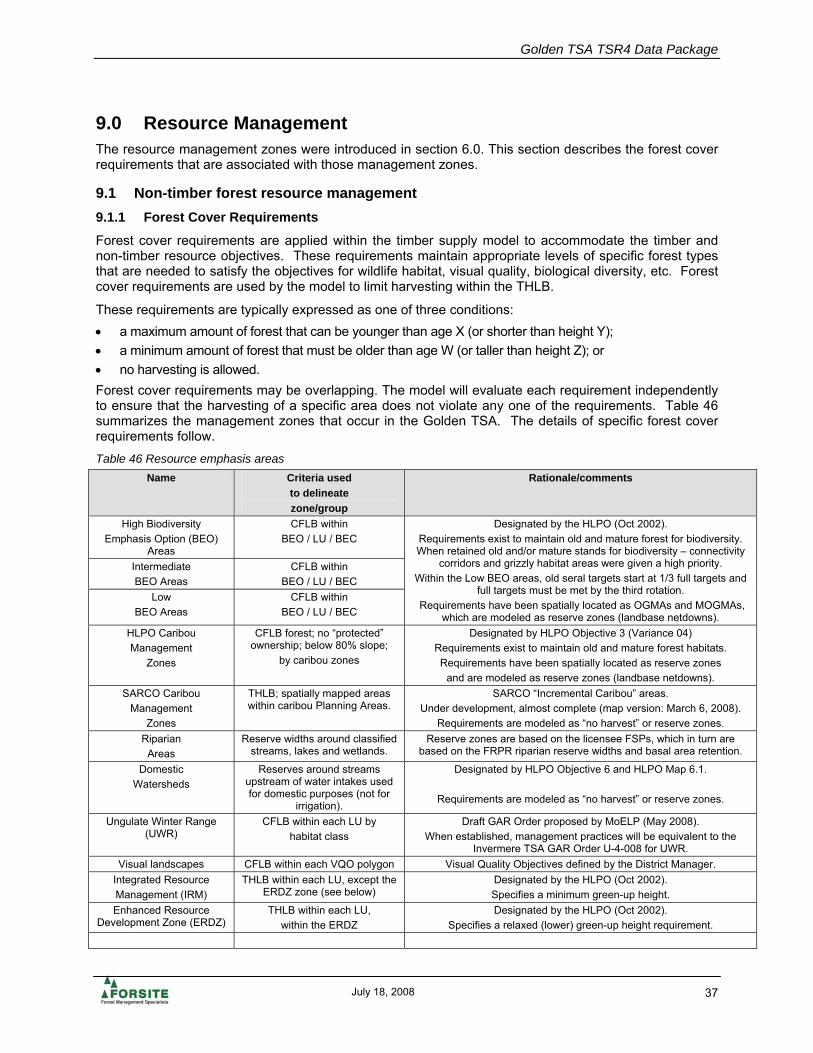
Golden TSA TSR4 Data Package
July 18, 2008 37
9.0 Resource Management The resource management zones were introduced in section 6.0. This section describes the forest cover requirements that are associated with those management zones.
9.1 Non-timber forest resource management 9.1.1 Forest Cover Requirements
Forest cover requirements are applied within the timber supply model to accommodate the timber and non-timber resource objectives. These requirements maintain appropriate levels of specific forest types that are needed to satisfy the objectives for wildlife habitat, visual quality, biological diversity, etc. Forest cover requirements are used by the model to limit harvesting within the THLB.
These requirements are typically expressed as one of three conditions: • a maximum amount of forest that can be younger than age X (or shorter than height Y); • a minimum amount of forest that must be older than age W (or taller than height Z); or • no harvesting is allowed. Forest cover requirements may be overlapping. The model will evaluate each requirement independently to ensure that the harvesting of a specific area does not violate any one of the requirements. Table 46 summarizes the management zones that occur in the Golden TSA. The details of specific forest cover requirements follow. Table 46 Resource emphasis areas
Name Criteria used to delineate zone/group
Rationale/comments
High Biodiversity Emphasis Option (BEO)
Areas
CFLB within BEO / LU / BEC
Intermediate BEO Areas
CFLB within BEO / LU / BEC
Low BEO Areas
CFLB within BEO / LU / BEC
Designated by the HLPO (Oct 2002). Requirements exist to maintain old and mature forest for biodiversity. When retained old and/or mature stands for biodiversity – connectivity
corridors and grizzly habitat areas were given a high priority. Within the Low BEO areas, old seral targets start at 1/3 full targets and
full targets must be met by the third rotation. Requirements have been spatially located as OGMAs and MOGMAs,
which are modeled as reserve zones (landbase netdowns). HLPO Caribou Management
Zones
CFLB forest; no “protected” ownership; below 80% slope;
by caribou zones
Designated by HLPO Objective 3 (Variance 04) Requirements exist to maintain old and mature forest habitats. Requirements have been spatially located as reserve zones
and are modeled as reserve zones (landbase netdowns). SARCO Caribou
Management Zones
THLB; spatially mapped areas within caribou Planning Areas.
SARCO “Incremental Caribou” areas. Under development, almost complete (map version: March 6, 2008).
Requirements are modeled as “no harvest” or reserve zones. Riparian Areas
Reserve widths around classified streams, lakes and wetlands.
Reserve zones are based on the licensee FSPs, which in turn are based on the FRPR riparian reserve widths and basal area retention.
Domestic Watersheds
Reserves around streams upstream of water intakes used for domestic purposes (not for
irrigation).
Designated by HLPO Objective 6 and HLPO Map 6.1.
Requirements are modeled as “no harvest” or reserve zones.
Ungulate Winter Range (UWR)
CFLB within each LU by habitat class
Draft GAR Order proposed by MoELP (May 2008). When established, management practices will be equivalent to the
Invermere TSA GAR Order U-4-008 for UWR. Visual landscapes CFLB within each VQO polygon Visual Quality Objectives defined by the District Manager.
Integrated Resource Management (IRM)
THLB within each LU, except the ERDZ zone (see below)
Designated by the HLPO (Oct 2002). Specifies a minimum green-up height.
Enhanced Resource Development Zone (ERDZ)
THLB within each LU, within the ERDZ
Designated by the HLPO (Oct 2002). Specifies a relaxed (lower) green-up height requirement.

Golden TSA TSR4 Data Package
July 18, 2008 38
Table 47 Resource emphasis areas – modeling constraints Name Crown
Forested Area (ha)
THLB Area (ha)
Forest resource requirements.
High Biodiversity Emphasis Option (BEO)
Areas 107,9281 23,6631
Intermediate BEO Areas
109,0011 55,7751
Old seral: no harvest within spatial OGMAs.
Mature-plus-old seral: no harvest within spatial MOGMAs.
Biodiversity: Low BEO Areas
209,4881 62,0921
Old seral: no harvest within spatial OGMAs for first rotation; apply a seral percentage requirement at 2/3 full target for the second rotation; increase the seral requirement to (3/3) full target for the third rotation
onwards. Mature-plus-old seral: no harvest within spatially mapped MOGMAs.
Caribou Management
zones 21,690 0
HLPO: No harvest within spatially mapped caribou areas. SARCO: No harvest within spatially mapped caribou areas.
Riparian Areas
13,125 0 Reserves around classified streams, lakes and wetlands.
Domestic or Sensitive Watersheds
322 0 Reserves around portions of streams upstream of intakes.
Ungulate Winter Range (UWR) 49,566 31,546
MF - dry: min 10% > 100 years MF – dry: min 10% >100 years MF – trans: min 10% >60 years
MF – trans: min 10% >100 years; S,F leading MF – mesic: min 10% >60 years
MF – mesic: min 20% >100 years; S,F leading MF – moist: min 20% >60 years MF – wet: min 30% >60 years
Visual landscapes 36,152 20,036 Maximum of X% < visual greenup age of Y,
applied within each VQO class within each LU. Integrated Resource
Management 98,210 98,210 Maximum of Max. 25% < 2.5 m tall. within LU / IRM zone
Enhanced Resource Development Zone (ERDZ) 43,319 43,319 Maximum of 33%<2 yr within LU / ERDZ zone
Notes: 1 = These numbers are the area assigned to that BEO according to the HLPO, not the areas of the OGMAs/MOGMAs.
9.1.1.1 Green-up / Maximum disturbance
The HLPO contains green-up requirements that require a logged block to achieve a specific condition called green-up before adjacent areas can be logged. Green-up refers to the average height of the regenerating forest reaching a specified target. Green-up requirements can often be waived if licensees manage for patch size distributions specified in the HLPO and detailed in the Landscape Unit Planning Guide (MoF/MoE 1999). Modeling of adjacent cut-block green-up requirements was accomplished using forest level objectives, as opposed to block specific objectives, because this is consistent with the operational flexibility afforded by patch size management. Green-up requirements and the area of application are provided in Table 48. Table 48 Green-up requirements by management zone Management Zone Green-up
Requirement Modeled Green-up
Constraint Area to
Which it applies HLPO ERDZ Timber Zone
successful regeneration (stocked)
max 33% < 2 yr within LU/ERDZ THLB area inside the HLPO mapped ERDZ timber zone
Integrated Resource Management Zone
2.5 m tall trees Max. 25% < 2.5 m tall within LU/IRM THLB not in ERDZ zone

Golden TSA TSR4 Data Package
July 18, 2008 39
Age to green-up was determined by calculating a weighted average stand type for each of the zones and then evaluating the age/height relationship for the stand in SiteTools. The IRM zone was S leading with an average site index of 17.3 – giving an 21 year greenup period to reach 2.5 meters height. A 2 year regeneration delay is then added to this value.
9.1.2 Visual Resources In this analysis, forest cover requirements aimed at meeting these objectives were applied so that the amount of younger stands that can occur in visually sensitive areas was limited. The following procedure was used to model the visual quality objectives: All VQO polygons had maximum planimetric percent disturbance values assigned based on VQO class, (values provided in Table 49). Table 49 Visually sensitive areas: Maximum planimetric disturbance percentage
VQO Class Percent Alteration Preservation 1%
Retention 5% Partial Retention 15%
Modification 25%
VQO polygons within each VQO class within each LU had an area weighted average slope assigned and a “visually effective greenup” (VEG) height calculated according to Table 50 extracted from Procedures for Factoring Visual Resources into Timber Supply Analyses (MoF 1998). Table 50 Tree heights required for meeting visually effective green-up by percent slope
Slope Class (%) 0-5 6-10 11-15 16-20 21-25 26-30 31-35 36-45 46-50 51-55 56-60 60+
Tree Height (m)
3.0 3.5 4.0 4.5 5.0 5.5 6.0 6.5 7.0 7.5 8.3 8.5
Each LU-VQO-class group had the resulting forest cover objective applied to its crown forested area in the model (Table 51). For example, a VQO of Retention and an average slope of 32% would have the following objective: No more than 5% of the crown forested area in that LU and VQO class can be less than 6m tall.
The visually effective green-up heights for each polygon were translated into green-up ages for use during modeling. Age to green-up was calculated in Site Tools using a weighted average stand type. Visually effective greenup ages ranges from 17 to 22 years (plus 2 year regeneration delay), based on an Fd stand with a site index of 17.34.

Golden TSA TSR4 Data Package
July 18, 2008 40
Table 51 Area weighted slope and greenup height assigned to each LU and VQO combination LU VQO Avg. Slope
(%) Max
Non-Veg (%) Greenup Ht (m) (age a/b)
G14 M 33.228 25 6 (22/24) G14 PR 28.444 15 5.5 (21,23) G15 M 22.37 25 5 (20/22) G15 PR 19.437 15 4.5 (18/20) G16 M 19.378 25 4.5 (18/20) G16 PR 17.102 15 4.5 (18/20) G19 M 20.112 25 4.5 (18/20) G19 PR 16.592 15 4.5 (18/20) G20 M 25.217 25 5 (20/22) G20 PR 24.671 15 5 (20/22) G20 R 14.345 5 4 (17/19) G21 M 34.859 25 6 (22/24) G21 PR 26.681 15 5.5 (21,23) G22 M 29.774 25 5.5 (21,23) G22 PR 23.827 15 5 (20/22) G22 R 11.901 5 4 (17/19) G23 M 26.126 25 5.5 (21,23) G23 PR 15.708 15 4.5 (18/20) G23 R 11.835 5 4 (17/19) G24 M 32.461 25 6 (22/24) G25 PR 27.61 15 5.5 (21,23) G25 R 20.833 5 5 (20/22) G26 M 26.509 25 5.5 (21,23) G26 PR 26.438 15 5.5 (21,23) G26 R 22.534 5 5 (20/22)
Note: (age a/b) = (15/17) = 15 years to reach greenup height; 17 = age including 2 years regeneration delay
9.1.3 Recreation resources
Forest cover retention within the important recreation areas in the Golden TSA was addressed primarily through the netdown process associated with the riparian areas around the streams and lakes.
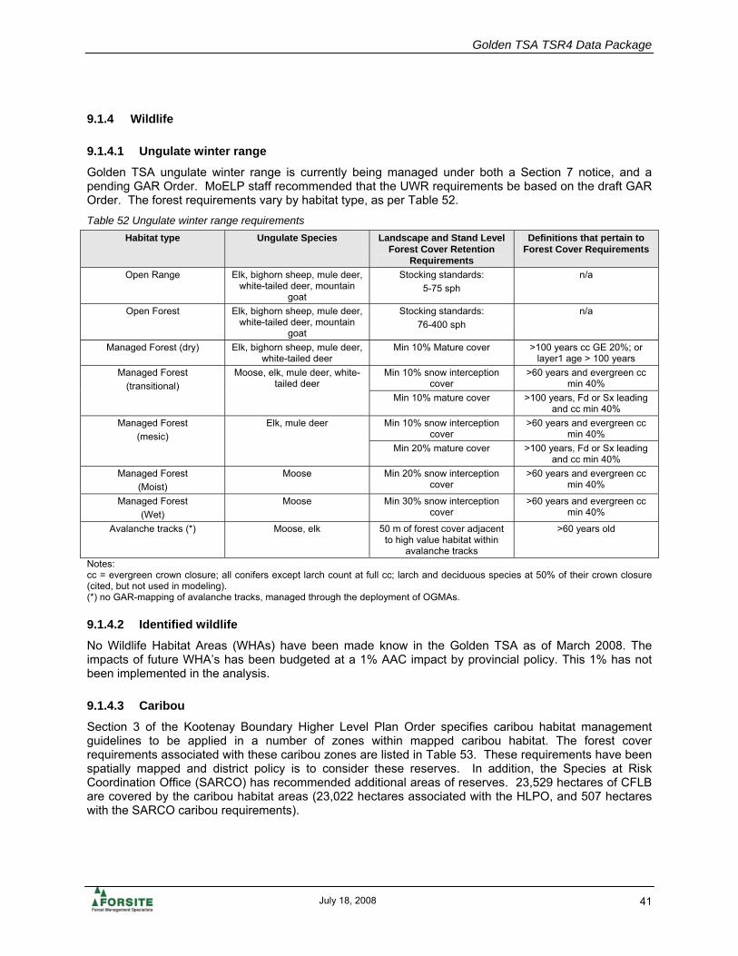
Golden TSA TSR4 Data Package
July 18, 2008 41
9.1.4 Wildlife
9.1.4.1 Ungulate winter range
Golden TSA ungulate winter range is currently being managed under both a Section 7 notice, and a pending GAR Order. MoELP staff recommended that the UWR requirements be based on the draft GAR Order. The forest requirements vary by habitat type, as per Table 52. Table 52 Ungulate winter range requirements
Habitat type Ungulate Species Landscape and Stand Level Forest Cover Retention
Requirements
Definitions that pertain to Forest Cover Requirements
Open Range Elk, bighorn sheep, mule deer, white-tailed deer, mountain
goat
Stocking standards: 5-75 sph
n/a
Open Forest Elk, bighorn sheep, mule deer, white-tailed deer, mountain
goat
Stocking standards: 76-400 sph
n/a
Managed Forest (dry) Elk, bighorn sheep, mule deer, white-tailed deer
Min 10% Mature cover >100 years cc GE 20%; or layer1 age > 100 years
Min 10% snow interception cover
>60 years and evergreen cc min 40%
Managed Forest (transitional)
Moose, elk, mule deer, white-tailed deer
Min 10% mature cover >100 years, Fd or Sx leading and cc min 40%
Min 10% snow interception cover
>60 years and evergreen cc min 40%
Managed Forest (mesic)
Elk, mule deer
Min 20% mature cover >100 years, Fd or Sx leading and cc min 40%
Managed Forest (Moist)
Moose Min 20% snow interception cover
>60 years and evergreen cc min 40%
Managed Forest (Wet)
Moose Min 30% snow interception cover
>60 years and evergreen cc min 40%
Avalanche tracks (*) Moose, elk 50 m of forest cover adjacent to high value habitat within
avalanche tracks
>60 years old
Notes: cc = evergreen crown closure; all conifers except larch count at full cc; larch and deciduous species at 50% of their crown closure (cited, but not used in modeling). (*) no GAR-mapping of avalanche tracks, managed through the deployment of OGMAs.
9.1.4.2 Identified wildlife
No Wildlife Habitat Areas (WHAs) have been made know in the Golden TSA as of March 2008. The impacts of future WHA’s has been budgeted at a 1% AAC impact by provincial policy. This 1% has not been implemented in the analysis.
9.1.4.3 Caribou
Section 3 of the Kootenay Boundary Higher Level Plan Order specifies caribou habitat management guidelines to be applied in a number of zones within mapped caribou habitat. The forest cover requirements associated with these caribou zones are listed in Table 53. These requirements have been spatially mapped and district policy is to consider these reserves. In addition, the Species at Risk Coordination Office (SARCO) has recommended additional areas of reserves. 23,529 hectares of CFLB are covered by the caribou habitat areas (23,022 hectares associated with the HLPO, and 507 hectares with the SARCO caribou requirements).

Golden TSA TSR4 Data Package
July 18, 2008 42
Table 53 Example of HLPO caribou forest cover requirements Caribou
Mngt. Zone
Zone Priority
Leading tree species
Minimum Forest retention
Min. Basal Area
Remaining
Minimum Forest
age class
Notes
1 1,2 Pl, Fd, or Lw 100% -- -- Previously harvested stands require future decisions
6 2 All Min 70% -- 8 8 2 All Min 30% -- 8 All Min 10% -- 9
8 2 All 20% Partial cut 70 7 Notes: Examples of HLPO caribou habitat zones and forest requirements. The equivalent area of the caribou requirements has been spatially mapped and is modeled as a THLB landbase reduction. 9.1.5 Biodiversity
The Landscape Unit Planning Guide (March 1999) provides background direction and guidance on biodiversity management. The Guide dictates that biodiversity be managed at both the landscape and stand levels. The primary mechanism for landscape-level management is retention of old and mature seral forest. Stand-level biodiversity is protected through retention of wildlife trees and wildlife patches. The following sections outline how retention of old and mature forest and wildlife trees/patches was modeled.
9.1.5.1 Landscape level biodiversity
Sections 1 and 2 of the Kootenay Boundary Higher Level Plan Order specify the amount of old and mature forest that must be maintained within each BEC variant inside each Landscape Unit (LU). Landscape units have been legally established along with Biodiversity Emphasis Option (BEO) assignments that guide the level of old/mature forest in each landscape unit.
Several Landscape Units overlap with portions of federal and provincial parks and protected areas. For the purposes of this analysis the productive forest area within all of LUs (with portions in parks and protected) are included in the analysis. The HLPO LU/BEC BEO assignments are listed in Table 54. Old and mature requirements for BEC/BEO combinations are provided in Table 55.

Golden TSA TSR4 Data Package
July 18, 2008 43
Table 54 LU/BEC BEO Assignments
LU BEO NDT BEC Area (ha) LU BEO NDT BEC Area (ha) G01 H 1 ESSFwc 2 4,466 G11 I 1 ESSFwc 2 1,996 G01 H 1 ESSFwcw 1,541 G11 I 1 ESSFwcw 853 G01 H 1 ICH wk 1 2,675 G11 I 1 ICH vk 1 1,242 G01 H 3 ESSFdk 1 2,710 G11 I 1 ICH wk 1 1,218 G02 I 1 ESSFvc 761 G12 H 1 ESSFwc 2 1,527 G02 I 1 ESSFwc 2 2,018 G12 H 1 ESSFwcw 950 G02 I 1 ESSFwcw 847 G12 H 1 ICH wk 1 2,342 G02 I 1 ICH vk 1 928 G13 H 1 ESSFvc 5,026 G02 I 1 ICH wk 1 3,110 G13 H 1 ESSFwc 2 3,988 G02 I 2 ICH mw 1 187 G13 H 1 ESSFwcw 1,768 G03 L 1 ESSFwc 2 2,935 G13 H 1 ICH wk 1 4,010 G03 L 1 ESSFwcw 1,446 G13 H 2 ICH mw 1 986 G03 L 1 ICH vk 1 2,119 G14 L 1 ESSFwc 2 6,802 G03 L 1 ICH wk 1 3,778 G14 L 1 ESSFwcw 1,831 G03 L 2 ESSFmm 1 339 G14 L 1 ICH wk 1 7,185 G03 L 2 ICH mw 1 1,334 G14 L 2 ICH mw 1 2,397 G04 I 1 ESSFwc 2 4,451 G15 L 1 ESSFwc 2 2,793 G04 I 1 ESSFwcw 2,754 G15 L 1 ESSFwcw 1,148 G04 I 1 ICH wk 1 5,173 G15 L 1 ICH wk 1 254 G04 I 2 ESSFmm 1 919 G15 L 2 ICH mw 1 5,020 G04 I 2 ICH mw 1 4,220 G16 I 1 ESSFwc 2 765 G06 H 1 ESSFwc 2 1,517 G16 I 2 ICH mw 1 23,533 G06 H 1 ESSFwcw 783 G16 I 3 ESSFdk 2 1,141 G06 H 1 ICH wk 1 1,835 G17 L 1 ESSFwc 2 3,648 G06 H 2 ICH mw 1 365 G17 L 1 ESSFwcw 1,233 G07 L 1 ESSFwc 2 4,224 G17 L 2 ICH mw 1 5,205 G07 L 1 ESSFwcw 1,537 G18 L 1 ESSFwc 2 2,524 G07 L 1 ICH wk 1 6,663 G18 L 1 ESSFwcw 710 G07 L 2 ICH mw 1 1,214 G18 L 2 ICH mw 1 3,591 G08 L 1 ESSFwc 2 3,738 G19 L 1 ESSFwc 2 4,771 G08 L 1 ESSFwcw 1,782 G19 L 1 ESSFwcw 1,488 G08 L 1 ICH wk 1 618 G19 L 1 ICH wk 1 552 G08 L 2 ICH mw 1 7,266 G19 L 2 ICH mw 1 5,455 G09 L 1 ESSFwc 2 4,092 G19 L 3 ESSFdk 2 920 G09 L 1 ESSFwcw 1,506 G20 I 1 ESSFwc 2 497 G09 L 2 ICH mw 1 6,222 G20 I 1 ESSFwcw 194 G10 L 1 ESSFwc 2 4,397 G20 I 2 ICH mw 1 8,126 G10 L 1 ESSFwcw 1,043 G20 I 3 ESSFdk 1 2,512 G10 L 1 ICH wk 1 3,269 G20 I 3 ESSFdk 2 2,526 G10 L 2 ICH mw 1 5,207 G20 I 3 ICH mk 1 1,786

Golden TSA TSR4 Data Package
July 18, 2008 44
(continued) LU BEO NDT BEC Area (ha) LU BEO NDT BEC Area (ha)
G20 I 3 MS dk 1,729 G26 H 3 MS dk 19,366 G20 I 4 IDF dm 2n 530 G26 L 2 ICH mw 1 2,857 G21 I 2 ICH mw 1 4,146 G26 L 3 ESSFdk 1 18,914 G21 L 3 ESSFdk 2 14,036 G26 L 3 ESSFdk 2 10,672 G21 L 3 ICH mk 1 8,456 G26 L 3 ICH mk 1 5,393 G22 I 2 ICH mw 1 6,456 G27 H 3 ESSFdk 1 3,947 G22 L 1 ESSFwm 5,418 G27 H 3 MS dk 4,357 G22 L 1 ICH wk 1 3,613 G28 H 3 ESSFdk 1 8,634 G22 L 3 ESSFdk 2 2,142 G28 H 3 ESSFdk 2 865 G23 I 2 ICH mw 1 8,701 G28 H 3 ESSFdku 394 G23 I 3 ESSFdk 2 6,216 G28 H 3 ICH mk 1 2,302 G23 I 3 ICH mk 1 8,017 G28 H 3 MS dk 22,337 G23 I 3 MS dk 1,448 G29 L 1 ESSFwc 2 2,927 G24 H 2 ICH mw 1 598 G29 L 1 ESSFwcw 1,100 G24 H 3 ESSFdk 2 4,150 G29 L 1 ICH wk 1 5,860 G25 L 3 ESSFdk 1 1,831 G29 L 2 ICH mw 1 261 G25 L 3 ESSFdk 2 277 G38 H 1 ESSFvc 179 G25 L 3 ICH mk 1 669 G38 H 1 ESSFwm 2,169 G25 L 3 MS dk 2,611 G38 H 1 ICH wk 1 2,143 G25 L 4 IDF dm 2n 192
Table 55 Old and mature forest cover requirements for landscape level biodiversity objectives
Mature+Old Seral Req Old Seral Requirements BEC Zone
NDT Mature Age (yrs)
Old Age (yrs)
Low Inter High Low * 1st Rot
Low * 2nd Rot
Low * 3rd Rot
Inter High
ESSFvc, ESSFwcw, ESSFwc2, ESSFwm
1 > 120 > 250 19 36 54 6.3 12.6 19 19 28
ICHvk1, ICHwk1 1 >100 >250 17 34 51 4.3 8.7 13 13 19 ESSFmm1 2 > 120 > 140 14 23 34 4.7 9.3 14 14 21 ICHmw1 2 > 100 > 250 15 31 46 3.0 6.0 9 9 13 ESSFdk, dku, ESSFdk1, dk2, ESSFdkw
3 > 120 > 140 14 23 34 4.7 9.3 14 14 21
ICHmk1 3 > 100 > 140 14 23 34 4.7 9.3 14 14 21 MSdk 3 > 100 > 140 14 26 39 4.7 9.3 14 14 21 IDF dm 2n 4 > 100 > 250 17 34 51 4.3 8.7 13 13 19 * Old seral requirements in Low BEO areas start at 1/3 old for first 80 years, 2/3 old for the next 80 years, and full old beyond for the Base Case (FRPA).
The target amount of old seral retention was calculated for each LU/BEO/BEC variant combination, and both old seral and mature-plus-old retention areas have been spatially identified and mapped as old growth management areas (OGMA) and mature and old management areas (MOGMA), respectively. Within the low biodiversity emphasis (BEO) areas only the 1/3 drawdown requirement for old seral has been mapped, as per the Higher Level Plan Order for the first rotation (assumed to be 80 years). In low BEO units the 2/3 target requirement and full (3/3) target requirements will be modeled as older seral retention requirements for the second and third rotations, respectively (i.e. in years 81-160, and 161 years+). The requirements are applied to the CFLB within each LU-BEC combination.

Golden TSA TSR4 Data Package
July 18, 2008 45
9.1.5.2 Disturbance of areas above the operability line
As crown forested stands in the non-THLB contribute toward several forest cover objectives (for example, landscape level biodiversity), it is important that the age class distributions in these stands remain consistent with natural processes. By implementing disturbance in these stands, a more natural age class distribution can be maintained in the model and a more realistic contribution toward seral goals ensured. To achieve this, a constant area was disturbed annually in each LU/NDT combination. The amount of disturbance is based on the BEC variants and their associated natural disturbance intervals and old seral definitions as outlined in the Biodiversity Guidebook (September 1995) and Table 56.
Using the negative exponential equation, the proportion of the forest that would typically occur as old seral forest can be calculated based on the disturbance interval (% area old = exp(-[old age / interval]). Using this % area in old, the calculation of an effective rotation age associated with this seral distribution was possible (Effective rotation age = interval / (1 – proportion old)). The effective rotation age can then be used to define an annual area of disturbance. For example, ESSF variants in NDT3 have a disturbance interval of 150 yrs and an old definition of 140 yrs. This translates into a typical age class distribution where 39% of the area is “old” (>140 yrs) and the oldest stands are around 230 years. Thus 1/230th of the area needs to be disturbed each year to maintain this age class distribution.
The Base Case includes: • Annual disturbance of the inoperable, contributing Non-THLB area. The selection of the stands to be
disturbed was determined by random selection. • OGMAs, plus the application of an old seral stage requirement to maintain a minimum amount of old
consistent with the % old targets wherever the target area had not been mapped as OGMAs in low BEO units.
This method is a slight simplification of Option 4 in ‘Modeling Options for Disturbance Outside the THLB - Working Paper’ (MoF, June 2003).
Table 56 Calculation of area to be disturbed annually in forested non-THLB by NDT / BEC
NDT
BEC
Age Old (yrs)
Return Interval
(yrs)
Prop- Ortion
Burned / Year
Effective Rotation
Age (yrs)
Disturbance ( proportion
per year) [A]
Contributing Non-THLB Area (ha)
[B]
Annual Area Disturbed By BEC [A} x [B]
1 ESSF 250 250 0.37 395 0.0025 91,898 232 1 ICH 250 250 0.37 395 0.0025 36,750 93 2 ESSF 200 250 0.29 350 0.0029 1,214 3 2 ICH 250 250 0.37 395 0.0025 38,451 97 3 ESSF 150 140 0.39 231 0.0043 69,919 303 3 ICH 150 140 0.39 231 0.0043 8,830 38 3 MS 150 140 0.39 231 0.0043 37,344 162 4 IDF 250 250 0.37 395 0.0025 483 1
Totals 930
The disturbance is implemented in the model using a random uniform probability. Each NDT is ‘turned over’ once during a period equal to its effective rotation age and then once again over the next effective rotation age, etc. There is no guarantee that any particular portion of the landbase will actually be disturbed in any one year. Across the NCLB, approximately 930 ha is disturbed each year (0.05%), resulting in an average ‘turning over’ of the landbase every ~ 306 years (range is 231 to 395 years).
9.1.5.3 Wildlife tree retention areas (WTRA)
Wildlife tree retention is one of the primary methods to address stand level biodiversity objectives. Section 3.2 and Appendix 3 of the Landscape Unit Planning Guide (March 1999) describe the process for determining wildlife tree retention requirements at the BEC sub-zone level in order to establish LU

Golden TSA TSR4 Data Package
July 18, 2008 46
objectives. On May 15, 2000, the Assistant Deputy Ministers of Forests and Environment, Lands and Parks approved changes to Section 3.2 of the Landscape Unit Planning Guide. Detailed policy on management of wildlife trees is provided in the document Provincial Wildlife Tree Policy and Management Recommendations (MoF/WLAP, February, 2000).
The Licensees’ FSPs are based on Section 66 (1) of the Forest and Range Practices Regulation (FRPR). Licensees are retaining, on an area basis, 7% of the total area of their cutblocks. When possible, retention is within non-THLB areas. Existing, mapped WTRA’s are removed from the THLB as landbase netdowns. These are within or adjacent to existing cutblocks.
The estimate of future WTRA’s was described in section 4.0
9.1.5.4 Coarse Woody Debris
Management of Coarse Woody Debris (CWD) is another factor in the management of stand level biodiversity. As per provincial policy, it was assumed that CWD objectives are managed operationally while meeting the harvest utilization standards.
9.1.5.5 Patch size objectives
Patch size management has been adopted in the Golden TSA in an effort to more closely mimic natural disturbance patterns and minimize fragmentation of the land base. Patch size management attempts to achieve the patch size distributions specified in the Landscape Unit Planning Guide (MoF/MoE 1999), and is an alternative to cut block adjacency green-up objectives. Cutblock green-up requirements (adjacency) are not modeled directly in this analysis because landscape level forest cover objectives are used to approximate these requirements. As patch management is also a spatial issue beyond the resolution of this timber supply analysis, the same landscape level objectives were used to approximate patch management requirements. In the opinion of the authors, spatial analyses completed in previous projects have confirmed that these landscape level forest cover objectives are consistent with the flexibility associated with patch size management and the operational application of green-up requirements.
9.1.5.6 Connectivity
The HLPO objectives for connectivity were incorporated while spatially locating the OGMAs and MOGMAs (4.14). Stands within the connectivity corridors were considered as a higher priority when allocating these old and mature forest retention areas. No further modeling was done for connectivity objectives.

Golden TSA TSR4 Data Package
July 18, 2008 47
9.1.6 Domestic Watersheds
The HLPO Objective 6 and HLPO Map 6.1. identify the water intakes where reserves are required around portions of the streams up-stream of the intakes for domestic water use (versus for purposes of irrigation). Streams are to be protected by a thirty meter reserve on each side of the stream for distance that depends on the stream order. Streams segments were mapped and reserves were modeled as “no harvest” areas in the base case, and hence are treated as THLB exclusions (Section 4.12).
9.1.7 Lakeshore, wetland and riparian management zones
In general, riparian management was predominately addressed through a netdown process that reflected both the reserve and management zones (Section 4.13).
9.2 Timber Harvesting 9.2.1 Minimum harvesting age / merchantability standards
For this analysis, minimum harvestable ages were defined by the following criteria: • minimum volume per hectare (200 m3/ha for C or H stands, or 150m3/ha for other species), and • minimum piece size (25 cm mean DBH, except for 20cm mean DBH for Pl stands), and • the age at which 95% of the culmination of the mean annual increment (CMAI) is achieved (Table 57). These merchantability criteria were adopted from TSR 3.
In order for the stand within the timber supply model to be considered for harvesting, it must achieve an age where the criteria described above are achieved. This ensures that the timber supply model is harvesting stands that meet reasonable economic criteria, and emulate what is generally current practice by forest licensees.
Note that these are minimum criteria, not the actual ages at which stands are forecast for harvest. Some stands may be harvested at the minimum thresholds to meet forest-level objectives while other stands may be not be harvested until well past there "optimal" timber production ages due to management objectives for other resource values, such as requirements for the retention of older forest or ungulate winter range. The minimum harvest age to be utilized for each analysis unit is defined in Table 58 and Table 59.
Table 57 Minimum merchantability rules
Leading Species
Minimum Volume (m3/ha)
Minimum DBH (cm)
Percent of Culmination
C, H 200 25 95 Pine 150 20 95
Decid (logged) 100 25 95 Other 150 25 95
Notes: The low value for deciduous, previously logged stands (AU = 123) assumes some form of stand rehabilitation, otherwise the minimum harvest age, if based on a minimum of 150 m3/ha, will be 245 years.

Golden TSA TSR4 Data Package
July 18, 2008 48
Table 58 Minimum age to reach merchantability criteria
Age to Reach Age to Reach Description
AU Nat Min
DBH Min Vol
95% MAI
MHA
AU Man Min
DBH Min Vol
95% MAI
MHA
Fd (dry), Lw 101 50 56 76 76 201 30 37 50 50 Fd (dry), Lw 102 60 76 93 93 202 50 56 68 68 Fd (dry), Lw 103 n/a n/a n/a n/a 203 n/a n/a n/a n/a Fd (wet), Lw 104 50 46 75 75 204 30 37 53 53 Fd (wet), Lw 105 60 66 85 85 205 50 57 70 70 Fd (wet), Lw 106 70 76 95 95 206 70 66 82 82
Cw 107 50 66 68 68 207 40 46 75 75 Cw 108 60 86 74 86 208 60 66 92 92 Cw 109 80 115 80 115 209 70 76 103 103 Hw 110 50 66 69 69 210 40 46 72 72 Hw 111 70 76 81 81 211 60 66 92 92 Hw 112 80 116 118 118 212 80 86 119 119 B, S 113 60 56 74 74 213 40 47 59 59 B, S 114 70 76 93 93 214 50 66 86 86 B, S 115 100 105 128 128 215 80 86 118 118
S - mixed 116 50 56 73 73 216 30 37 58 58 S – mixed 117 60 66 85 85 217 40 57 73 73 S – mixed 118 80 86 108 108 218 60 66 99 99
Pine 119 50 46 55 55 219 20 37 47 47 Pine 120 60 46 60 60 220 30 36 53 53 Pine 121 70 66 71 71 221 30 46 62 62 Pine 122 80 76 84 84 222 40 66 68 68 Decid 123 80 95 71 95 223 40 47 58 58
Table 59 Minimum age to reach merchantability- Existing Managed Stands
Age to Reach Age to Reach Description
AU Nat Min
DBH Min Vol
95% MAI
MHA
AU Man Min
DBH Min Vol
95% MAI
MHA
Fd (dry), Lw 501 60 66 79 79 601 50 56 74 74 Fd (wet), Lw 502 50 56 79 79 602 50 56 79 79
Cw 503 50 57 81 81 603 50 57 79 79 Hw 504 50 56 90 90 604 50 56 88 88 B, S 505 50 56 84 84 605 50 56 78 78
S mixed 506 60 66 90 90 606 60 56 69 69 Pine 507 40 56 68 68 607 40 56 66 66
Decid 508 40 47 64 64 608 40 47 64 64 Backlog 1 525 70 86 110 110 625 50 56 75 75 Backlog 2 526 70 78 115 115 626 40 57 69 69

Golden TSA TSR4 Data Package
July 18, 2008 49
9.2.2 Operability / harvest systems
An operability line separates the operable and inoperable portions of the Golden TSA. The last complete operability mapping project was completed in 2002. A minor update was completed in April, 2008 by the forest licensees and that version is used in this analysis.
Any past harvesting above the 2008 operability line is considered as inoperable in this analysis.
9.2.3 Initial Harvest Rate
The Base Case harvest forecast will use 492,627 as the initial harvest rate, based on:
485 000 m3/yr [A] + 7,627 m3/yr [B] = 492 627 /yr [C]
Where: [A] = current AAC, [B] = un-salvaged losses, [C] = initial harvest rate.
9.2.4 Harvest rules
Harvest rules have the objective of influencing the model so the harvest profile in the model will reasonably match the harvest profile seen on-the-ground. Licensees don’t necessarily follow an “oldest-first” harvest priority. Numerous pressures influence forest operations and the harvest profile may vary greatly between 5-year periods. The more notable examples are the recent bark beetle infestations and fires.
To reflect the current concentration on harvesting to control the MPB, the harvest priority rules in Table 60 were adopted for the Base Case scenarios.
Harvest Priorities are: (1) relative-oldest first; (2) intent is to cap % pine in harvest at 70%; then (3) prioritize within groups: (a) Pine; (b) fir; then (c) other species.
Table 60 Harvest priority rules
Harvest priority Description Overall harvest priority;
Cover constraints Relative oldest first harvest rule; and
Ensure all forest cover requirements are met at all times. Susceptible to
Mountain pine beetle stands Highest priority is lodgepole pine leading stands, with a
maximum of 70% of the harvest to come from Pl leading stands; then Fir-leading stands Fir-leading leading stands; then
Other species Other stands in the THLB.
9.2.5 Harvest profile
No specific harvest profile was modeled, although pine-leading stands are expected to dominate due to a priority placed on harvesting pine-leading stands before other species (above). The maximum contribution of pine-leading stands to the harvest was capped at 70% each model period (each decade, unless otherwise specified).
9.2.6 Silviculture Systems
Silviculture systems are predominately clearcut and clearcut-with-reserves, with negligible areas of partial cutting. Partial cutting is employed largely within the visual landscapes. This was deemed to be too minor to model separately. In the past, partial cutting was used within pine-salvage stands but this practice is no longer followed, and re-entries into past salvage stands have set these stands into a clearcut management regime.
Planting is by far the predominant method of regeneration. Natural regeneration was modeled only in the existing, backlog NSR stands.

Golden TSA TSR4 Data Package
July 18, 2008 50
9.2.7 Harvest flow objectives
Except for the sensitivity analyses where alternate harvest flow objectives are examined, the objectives for harvest flow in the Base Case are: • Initially, start at the current AAC, • Maintain the current AAC for as long as possible (the intent is that the mid-term harvest level will not be
reduced to below the LTSY level), and • If necessary, reduce the harvest flow at a maximum rate of 10% in any one decade, • If necessary, minimize the length of any fall-down period, • When possible, increase the harvest flow at a maximum rate of 10% per decade, and • Reach a stable, long-term harvest flow rate associated with a constant (flat line) total inventory. Modeling will be performed for at least 300 years, using 10-year periods, and reporting will be for the first 250 years.

Golden TSA TSR4 Data Package
July 18, 2008 51
10.0 Timber Supply Modeling and Forecasts This section provides a summary of the modeling which will be completed following the acceptance of the Data Package. This includes the model and the intended harvest forecasts that will be completed, and which will then be documented in the TSR Analysis Report.
10.1 Model Forest Planning Studio (FPS) version 6.0.2.0 will be used to complete the timber supply analysis. FPS was developed by Dr. John Nelson at the University of British Columbia (UBC) and is a spatially explicit forest estate simulation model. All events in the model are directly linked to stand level polygons or harvest units and thus allow tracking of individual stand attributes and spatial relationships through time. Each polygon belongs to a specific stand type (Analysis Unit) and has attributes such as age, harvest system, and land base status (THLB or Non THLB). Results are typically aggregated for reporting at higher levels (i.e. harvest flow for the entire unit).
A wide range of constraints can be modeled on the land base: harvest exclusion, spatial adjacency/maximum cutblock size, maximum disturbance/young seral, minimum mature/old seral, and equivalent clearcut area (ECA) limits. Constraints are applied to groups of polygons (cliques) and harvest is restricted if a constraint is not satisfied. A single polygon can belong to many overlapping cliques and each of them must be satisfied in order to allow harvest of the polygon. Where a mature or old cover constraint is not met, harvesting may still occur if there are any eligible stands remaining after the oldest stands are reserved to meet the constraint.
Harvest is implemented using a set of priorities to queue stands for harvest. In each period, the model harvests the highest priority eligible stands until it reaches the harvest target or exhausts the list of opportunities. Harvest can be implemented in single years, multiple year periods or a combination of these. Where periods are used, the midpoint of the period is typically used as the point where harvest opportunity is evaluated because it is a good balance between the start of the period (pessimistic) and the end of the period (optimistic).
10.2 Base Case The Base Case is based on current management practices within the Golden TSA. This is defined by operational management practices, characteristics of and natural resource values found on the landbase, current silviculture practices, and estimates of present and future growth of forest stands. The preceding sections described the assumptions and data that are included in the Base Case.
10.3 Sensitivity Analyses Sensitivity runs are used to test the uncertainty inherent in the data and management assumptions and are performed by modifying one input and examining the impact that change has on the model outputs. The sensitivity runs provide a picture of what factors in the Base Case are most influential, in relative terms, to the outputs. Table 61 is the list of proposed sensitivity analyses.

Golden TSA TSR4 Data Package
July 18, 2008 52
Table 61 Base Case sensitivity analyses.
Parameter Adjusted Definition Number of Runs Natural stand yields Natural stand yields +/- 10% 2
Managed stand yields Managed stand yields +/- 10% 2 Regeneration delay Regeneration delay +2 / -1 years 2
Minimum harvest age
(MHA) Base case values +/- 10 years 2
MHA (volume criteria only)
New values based on minimum volume criteria only 2
MHA (MAI criteria only) New values based on attaining maximum mean annual increment only
2
Timber harvesting landbase
Increase/decrease landbase by 10% 2
Genetic gains Managed stand yields without genetic gains 1 Totals 15
10.4 Alternate harvest flows over time The harvest flow is the estimated rate of harvest for each period (10 years/period) over a long term planning horizon (250 years or more). There are many possible harvest flows with different starting harvest levels, and with different rates of declining and/or increasing harvests between periods. For example, it is possible to ‘trade off’ the mid- or long-term harvest for short-term harvest, or vice versa. A number of harvest flows will be produced for the Base Case option (Table 62). These provide a picture of the trade-offs that were inherent in developing the recommended harvest flow.
Table 62 Alternate Base Case harvest flows Alternate Harvest Flow Key parameters Number
of runs Maximum starting
harvest level Highest possible starting level with a
maximum decline per decade not to exceed 10% of the previous decade. 1
Maintain current AAC
Maintain, for as long as possible, the current AAC without any decline. Maintain the mid-term harvest level, if possible, above the long term sustained yield.
1
Non-declining even flow. Maximum harvest level with no decline in harvest in any period. 1 Totals 3

Golden TSA TSR4 Data Package
July 18, 2008 53
10.5 Other options Other options are used to quantify the impacts of alternate management, or combinations of modeling assumptions that are significantly different than the Base Case. Table 63 summarizes the options that will be examined. Table 63 Other Options
Option Key management parameters Non-spatial Biodiversity and
Caribou Option (“Non-spatial Option”)
Non-spatial Biodiversity and Caribou Option – Assume that spatially deployed biodiversity OGMAs and Mature; and spatially deployed HLPO-related caribou were not available. Model the requirements as aspatial (percentage) older forest requirements. The intent is to quantify the effect, if any, of the spatial mapping.
Mountain Pine Beetle Option
(“MPB Option”)
Mountain Pine Beetle Option - Assume catastrophic MPB attack levels as forecast by Ministry of Forest staff (Eng et al, 2005). The intent is to explore a worst-case scenario where almost all Pl volume is lost in a very short time frame. The goal would be to capture as much of the attacked pine as possible under an AAC uplift before it becomes uneconomic to salvage, and then, reduce the harvest to a long term sustainable level.
Split-TSA Harvest Flow (“MPB Option”)
Split-TSA Harvest Flow Option – This option will examine harvest flows from three portions of the TSA: north, mid and south. The intent is to examine the wood supply that flows north and west to Revelstoke versus that which flows south to Golden. The “mid” portion could flow either north or south.
10.6 Non-spatial OGMA and Caribou Option This option is designed to show the timber supply implications of modeling the caribou, and the biodiversity seral requirements as aspatial older seral requirements. The differences between the Base Case and this option are:
• The mapped areas that representing the HLPO aspatial caribou requirements are “turned off” and are replaced with aspatial, older seral requirements. The SARCO caribou “incremental” areas remain as no harvest areas, or THLB netdowns (no change from Base Case).
• OGMAs and MOGMAs are “turned off” and biodiversity targets are modeled as older seral requirements, as per the HLPO. In the low BEO areas, starting in the first rotation, the old seral requirements start at 1/3-target levels and increase to full targets by the end of three rotations. (*) = modeled as THLB reductions
10.6.1 Old growth management areas
In the base case, the required area of old seral retention was calculated for each LU/BEO/BEC variant combination and old seral retention areas have been spatially identified and mapped as old growth management areas (OGMAs) and mature-plus-old management areas (MOGMAs). In this option the OGMAs and MOGMAs are replaced with aspatial seral requirements. The effect is seen in the landbase netdown table (Table 64).
10.6.2 Caribou management areas
In the base case, the required area of older forest types was calculated and equivalent area was spatially identified and mapped as caribou reserves. In this option the caribou reserves are replace with the HLPO caribou seral requirements. The effect is a significant increase in the timber harvesting landbase (Table 64).

Golden TSA TSR4 Data Package
July 18, 2008 54
Table 64 Landbase Comparisons – Base Case and Non-spatial Biodiversity and Caribou Option
Base Case Scenario
(ha)
Non-spatial Biod and Caribou
(ha) (*) Total land base 1,184,611 1,184,611
Reductions Private, Woodlots, non-contributing
administrative classes 22,975 22,975 Non-forest, non-productive forest 724,882 724,882
Roads, trails, landings 4,077 4,077 Total productive land base (*) 432,677 432,677
Reductions Parks and protected areas (**) 88,227 88,227
Inoperable 165,829 165,829 Unstable terrain (ESA & TSIL) 3,376 3,376
Non-merch (low site) 3,067 3,067 PFT (Hw and Decid) 5,548 5,548
Wildlife (caribou HLPO and SARCO) 8,348 0 Archaeological sites 0 0
Riparian 5,194 5,367 Biodiversity - WTRA 1,543 1,651
Biodiversity – OGMA and MOGMA 9,910 0 Permanent sample plots 105 120
Total Reductions 291,147 273,185 Current Timber Harvesting Land Base 141,530 159,492
Future WTPs 652 652 Future roads and trails 2,516 2,836
Net long-term Timber Harvesting Land Base 138,362 156,004 Note: 1. All totals are subject to rounding. 2. (*) Some Park area is included for biodiversity modeling on the productive landbase. Totals below (**) do not include any of this Park area. Note that any overlaps between net-downs are removed in the table. Any overlap will accrue to the first (highest) category in the table.
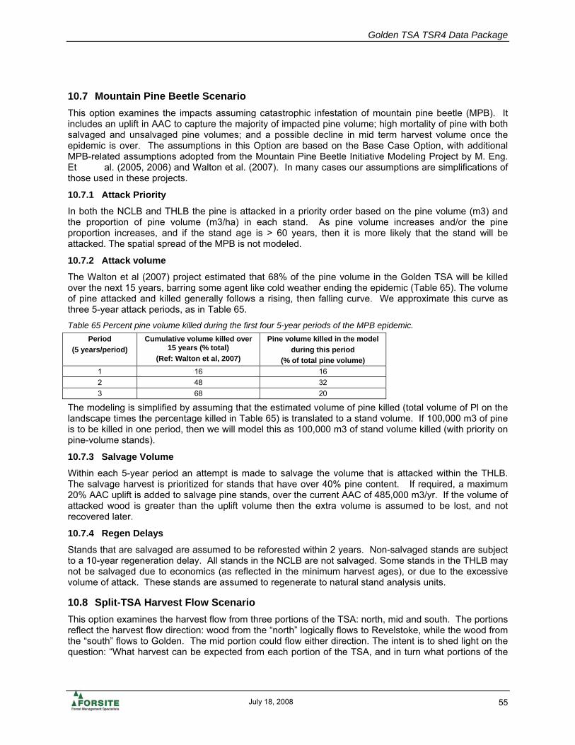
Golden TSA TSR4 Data Package
July 18, 2008 55
10.7 Mountain Pine Beetle Scenario This option examines the impacts assuming catastrophic infestation of mountain pine beetle (MPB). It includes an uplift in AAC to capture the majority of impacted pine volume; high mortality of pine with both salvaged and unsalvaged pine volumes; and a possible decline in mid term harvest volume once the epidemic is over. The assumptions in this Option are based on the Base Case Option, with additional MPB-related assumptions adopted from the Mountain Pine Beetle Initiative Modeling Project by M. Eng. Et al. (2005, 2006) and Walton et al. (2007). In many cases our assumptions are simplifications of those used in these projects.
10.7.1 Attack Priority
In both the NCLB and THLB the pine is attacked in a priority order based on the pine volume (m3) and the proportion of pine volume (m3/ha) in each stand. As pine volume increases and/or the pine proportion increases, and if the stand age is > 60 years, then it is more likely that the stand will be attacked. The spatial spread of the MPB is not modeled.
10.7.2 Attack volume
The Walton et al (2007) project estimated that 68% of the pine volume in the Golden TSA will be killed over the next 15 years, barring some agent like cold weather ending the epidemic (Table 65). The volume of pine attacked and killed generally follows a rising, then falling curve. We approximate this curve as three 5-year attack periods, as in Table 65. Table 65 Percent pine volume killed during the first four 5-year periods of the MPB epidemic.
Period (5 years/period)
Cumulative volume killed over 15 years (% total)
(Ref: Walton et al, 2007)
Pine volume killed in the model during this period
(% of total pine volume) 1 16 16 2 48 32 3 68 20
The modeling is simplified by assuming that the estimated volume of pine killed (total volume of Pl on the landscape times the percentage killed in Table 65) is translated to a stand volume. If 100,000 m3 of pine is to be killed in one period, then we will model this as 100,000 m3 of stand volume killed (with priority on pine-volume stands).
10.7.3 Salvage Volume
Within each 5-year period an attempt is made to salvage the volume that is attacked within the THLB. The salvage harvest is prioritized for stands that have over 40% pine content. If required, a maximum 20% AAC uplift is added to salvage pine stands, over the current AAC of 485,000 m3/yr. If the volume of attacked wood is greater than the uplift volume then the extra volume is assumed to be lost, and not recovered later.
10.7.4 Regen Delays
Stands that are salvaged are assumed to be reforested within 2 years. Non-salvaged stands are subject to a 10-year regeneration delay. All stands in the NCLB are not salvaged. Some stands in the THLB may not be salvaged due to economics (as reflected in the minimum harvest ages), or due to the excessive volume of attack. These stands are assumed to regenerate to natural stand analysis units.
10.8 Split-TSA Harvest Flow Scenario This option examines the harvest flow from three portions of the TSA: north, mid and south. The portions reflect the harvest flow direction: wood from the “north” logically flows to Revelstoke, while the wood from the “south” flows to Golden. The mid portion could flow either direction. The intent is to shed light on the question: “What harvest can be expected from each portion of the TSA, and in turn what portions of the

Golden TSA TSR4 Data Package
July 18, 2008 56
TSA should be expected to flow north to Revelstoke vs. south to Golden. This option is identical to the Base Case, except that sub-TSA harvest flow controls will be applied to each portion of the TSA.
11.0 References Eng, M., Andrew Fall, Josie Hughes, Terry Shore, Bill Riel, Peter Hall, and Adrian Walton. 2005. Provincial-Level
Projection of the Current Mountain Pine Beetle Outbreak: An Overview of the Model (BCMPB v2) and Results of Year 2 of the Project. Mountain Pine Beetle Initiative of the Canadian Forest Service and the BC Forest Service. April 2005.
Eng, M., Andrew Fall, Josie Hughes, Terry Shore, Bill Riel, Adrian Walton, and Peter Hall. 2006. Provincial-Level Projection of the Current Mountain Pine Beetle Outbreak: Update of the infestation projection based on the 2005 Provincial Aerial Overview of Forest Health and revisions to the model (BCMPB.v3). http://www.for.gov.bc.ca/hre/bcmpb/ April 21, 2006
Forest Practices Board. 2008. (Draft) Audit of Soil Conservation Columbia Forest District. Audit Report. (Draft ) May 2008.
Government of British Columbia. 1995. Biodiversity Guidebook.
Government of British Columbia. 1995. Riparian Management Area Guidebook.
Government of British Columbia. 1999. Landscape Unit Planning Guide.
Government of B.C. 2002. Kootenay-Boundary Higher Level Plan Order. B.C. Ministry of Sustainable Resources. October 26, 2002. http://srmwww.gov.bc.ca/kor/rmd/docs/nov4_2002/KBHLPOrder0925.pdf
Government of British Columbia. 2002. Forest and Range Practices Act
Government of British Columbia. 1995. Forest Practices Code of British Columbia Act
Government of British Columbia. 2006. Notices for UWR. Website: ftp://ribftp.env.gov.bc.ca/pub/outgoing/cdc_data/Approved_FRPR_sec7_WLPPR_sec9_Notices_and_Supporting_Info/UWR/Tree_Farm_Licenses/TFL_14/ and ftp://ribftp.env.gov.bc.ca/pub/outgoing/cdc_data/Approved_FRPR_sec7_WLPPR_sec9_Notices_and_Supporting_Info/Species_at_Risk/Rocky_Mountain_FD/
Jahraus & Associates, and Churlish Consulting Ltd. 2007. Golden TSA. Documentation of Analysis for Vegetation Resources Inventory Statistical Adjustment And Net Volume Adjustment Factor Development. Report PREPARED FOR LOUISIANA-PACIFIC CANADA LTD., Golden. PREPARED BY Jahraus & Associates Consulting Inc., Maple Ridge BC, And Churlish Consulting Ltd., Victoria BC. MARCH 2007
Holmes, Peter. 2008. Personal communication. Ecosystems Biologist, Ministry of Environment, Invermere.
Kootenay Inter-Agency Management Committee. 1997. Kootenay-Boundary Land Use Plan Implementation Strategy. Land Use Coordination Office.
Mah, Shirley. 2007. Personal communication. Interpretations Ecologist, Ministry of Forests, Victoria.
Ministry of Environment, Environmental Stewardship Division. Identified Wildlife Handbook web site: http://www.env.gov.bc.ca/wld/identified/index.html
Ministry of Environment and Ministry of Forests (MoE/MoF). 1999. Managing Identified Wildlife: Procedures and measures. Forest Practices Code of BC. February 1999. Web site address: http://www.env.gov.bc.ca/wld/identified/index.html
Ministry of Forests. 1996 Nelson Forest Region Technical Report MIT-003, Effect of Silviculture Practices on Green-up Delay in the Nelson Forest Region
Ministry of Forests. 1997. Visual impacts of partial cutting. Summary Report. A Technical Analysis and Public Perception Study. B.C. Ministry of Forests, Forest Development Section, Forest Practices Branch. August 1997.
Ministry of Forests. 1998. Procedures for Factoring Visual Resources into Timber Supply Analyses. Forest Practices Branch and Timber Supply Branch. March 17, 1998
Ministry of Forests. 2003a. Bulletin: Modelling Visuals in TSR III. Update to 'Procedures for Factoring Visual Resources into Timber Supply Analyses'. December 12 2003.

Golden TSA TSR4 Data Package
July 18, 2008 57
Ministry of Forests. 2003b. Modeling Options for Disturbance Outside the THLB - Working Paper. Timber Supply Branch, Ministry of Forests, June 2003.
Ministry of Forests. 2004. Chief Forester’s Standards for Seed Use. Ministry of Forests. November 20, 2004 Amended November 23, 2006.
Ministry of Forests. 2007. Glossary of Statistical Reporting Terms. Timber Supply Branch. Web site address: http://www.for.gov.bc.ca/hts/inventory/reports/glossary/index.html
Monchak, Darcy. 2004. Golden TSA LU Deployment Tables. Excel summary tables. December, 2005. Prepared by Darcy Monchak, R.P.F., MSRM, Southern Interior Region.
Monchak, Darcy. 2005. Spatial Deployment Of KBHLP Biodiversity And Caribou Objectives For The Golden TSA, Documentation of Procedures and Results. Version 1.2, January 17, 2005. Prepared by Darcy Monchak, R.P.F., MSRM, Southern Interior Region.
Nigh, G.D. 2007. Personal communication. Leader, Strategic Analysis, Ministry of Forests, Victoria.
Nigh, G.D. and B.A. Love. 1998. A Model for Estimating Juvenile Height of Lodgepole Pine
Nigh, G.D. 1995. Site Index Conversion Equations for Mixed Species Stands
Walton, A., Josie Hughes, Marvin Eng, Andrew Fall, Terry Shore, Bill Riel, and Peter Hall. 2007. Provincial-Level Projection of the Current Mountain Pine Beetle Outbreak: Update of the infestation projection based on the 2006 Provincial Aerial Overview of Forest Health and revisions to the "Model" (BCMPB.v4). http://www.for.gov.bc.ca/hre/bcmpb/ April 30, 2007

Golden TSA TSR4 Data Package
July 18, 2008 58
APPENDIX A. NATURAL STAND (VDYP) YIELD TABLES <insert tables after this page>

Lw, Fd (dry) - best Lw, Fd (dry) - mod
Analysis Unit Age Volume Diameter MAI Analysis Unit Age Volume Diameter MAI
101 0 0 0 0.0 102 0 0 0 0.0
101 10 0 0 0.0 102 10 0 0 0.0
101 20 0 2 0.0 102 20 0 0 0.0
101 30 23 20 0.8 102 30 1 6 0.0
101 40 76 22 1.9 102 40 26 19 0.7
101 50 129 24 2.6 102 50 62 22 1.2
101 60 180 26 3.0 102 60 99 23 1.7
101 70 229 28 3.3 102 70 135 25 1.9
101 80 275 30 3.4 102 80 169 27 2.1
101 90 318 32 3.5 102 90 201 28 2.2
101 100 355 34 3.6 102 100 232 30 2.3
101 110 386 36 3.5 102 110 261 32 2.4
101 120 414 38 3.5 102 120 286 34 2.4
101 130 440 40 3.4 102 130 309 35 2.4
101 140 461 42 3.3 102 140 328 37 2.3
101 150 481 44 3.2 102 150 346 38 2.3
101 160 498 45 3.1 102 160 360 39 2.3
101 170 513 47 3.0 102 170 373 41 2.2
101 180 526 49 2.9 102 180 385 42 2.1
101 190 538 50 2.8 102 190 396 44 2.1
101 200 550 52 2.8 102 200 407 45 2.0
101 210 561 54 2.7 102 210 417 46 2.0
101 220 572 55 2.6 102 220 426 48 1.9
101 230 582 57 2.5 102 230 435 49 1.9
101 240 591 59 2.5 102 240 444 51 1.9
101 250 600 61 2.4 102 250 452 52 1.8
101 260 600 61 2.3 102 260 452 52 1.7
101 270 600 61 2.2 102 270 453 52 1.7
101 280 599 61 2.1 102 280 453 52 1.6
101 290 599 61 2.1 102 290 453 52 1.6
101 300 598 61 2.0 102 300 453 53 1.5
101 310 597 61 1.9 102 310 453 53 1.5
101 320 597 61 1.9 102 320 453 53 1.4
101 330 596 61 1.8 102 330 452 53 1.4
101 340 595 61 1.8 102 340 452 53 1.3
101 350 593 61 1.7 102 350 452 53 1.3
Yield Tables

Lw, Fd (wet) - best Lw, Fd (wet) - mod
Analysis Unit Age Volume Diameter MAI Analysis Unit Age Volume Diameter MAI
104 0 0 0 0.0 105 0 0 0 0.0
104 10 0 0 0.0 105 10 0 0 0.0
104 20 0 4 0.0 105 20 0 1 0.0
104 30 25 20 0.8 105 30 2 12 0.1
104 40 88 22 2.2 105 40 41 21 1.0
104 50 153 24 3.1 105 50 91 22 1.8
104 60 215 26 3.6 105 60 139 24 2.3
104 70 273 28 3.9 105 70 184 26 2.6
104 80 327 30 4.1 105 80 226 27 2.8
104 90 376 32 4.2 105 90 265 29 2.9
104 100 420 34 4.2 105 100 301 31 3.0
104 110 457 36 4.2 105 110 334 33 3.0
104 120 489 39 4.1 105 120 363 34 3.0
104 130 519 41 4.0 105 130 390 36 3.0
104 140 547 42 3.9 105 140 413 38 3.0
104 150 571 44 3.8 105 150 434 39 2.9
104 160 594 46 3.7 105 160 453 40 2.8
104 170 614 48 3.6 105 170 470 42 2.8
104 180 633 49 3.5 105 180 486 43 2.7
104 190 650 51 3.4 105 190 500 44 2.6
104 200 666 53 3.3 105 200 514 46 2.6
104 210 682 54 3.2 105 210 527 47 2.5
104 220 696 56 3.2 105 220 540 49 2.5
104 230 710 58 3.1 105 230 551 50 2.4
104 240 724 60 3.0 105 240 563 51 2.3
104 250 736 61 2.9 105 250 573 53 2.3
104 260 738 61 2.8 105 260 575 53 2.2
104 270 739 62 2.7 105 270 577 53 2.1
104 280 741 62 2.6 105 280 578 53 2.1
104 290 742 62 2.6 105 290 579 53 2.0
104 300 743 62 2.5 105 300 581 54 1.9
104 310 744 62 2.4 105 310 582 54 1.9
104 320 745 63 2.3 105 320 583 54 1.8
104 330 745 63 2.3 105 330 584 54 1.8
104 340 746 63 2.2 105 340 585 54 1.7
104 350 747 63 2.1 105 350 586 55 1.7
Yield Tables

Lw, Fd (wet) - poorest Cw - best
Analysis Unit Age Volume Diameter MAI Analysis Unit Age Volume Diameter MAI
106 0 0 0 0.0 107 0 0 0 0.0
106 10 0 0 0.0 107 10 0 0 0.0
106 20 0 0 0.0 107 20 0 1 0.0
106 30 0 5 0.0 107 30 5 20 0.2
106 40 10 18 0.3 107 40 62 22 1.6
106 50 45 21 0.9 107 50 114 24 2.3
106 60 83 22 1.4 107 60 161 26 2.7
106 70 119 24 1.7 107 70 203 29 2.9
106 80 153 25 1.9 107 80 241 31 3.0
106 90 184 27 2.0 107 90 270 33 3.0
106 100 213 28 2.1 107 100 293 35 2.9
106 110 240 30 2.2 107 110 313 38 2.8
106 120 264 31 2.2 107 120 328 40 2.7
106 130 286 32 2.2 107 130 350 42 2.7
106 140 307 34 2.2 107 140 372 44 2.7
106 150 325 35 2.2 107 150 392 46 2.6
106 160 341 36 2.1 107 160 410 48 2.6
106 170 355 37 2.1 107 170 427 50 2.5
106 180 369 38 2.1 107 180 443 52 2.5
106 190 382 39 2.0 107 190 458 53 2.4
106 200 395 40 2.0 107 200 473 55 2.4
106 210 407 41 1.9 107 210 487 57 2.3
106 220 419 43 1.9 107 220 503 58 2.3
106 230 430 44 1.9 107 230 520 60 2.3
106 240 441 45 1.8 107 240 535 61 2.2
106 250 451 46 1.8 107 250 550 62 2.2
106 260 453 46 1.7 107 260 551 62 2.1
106 270 455 46 1.7 107 270 553 63 2.0
106 280 456 46 1.6 107 280 554 63 2.0
106 290 458 47 1.6 107 290 555 64 1.9
106 300 459 47 1.5 107 300 556 64 1.9
106 310 461 47 1.5 107 310 557 64 1.8
106 320 462 47 1.4 107 320 558 65 1.7
106 330 463 47 1.4 107 330 558 65 1.7
106 340 464 47 1.4 107 340 559 65 1.6
106 350 465 48 1.3 107 350 560 66 1.6
Yield Tables

Cw - mod Cw - poorest
Analysis Unit Age Volume Diameter MAI Analysis Unit Age Volume Diameter MAI
108 0 0 0 0.0 109 0 0 0 0.0
108 10 0 0 0.0 109 10 0 0 0.0
108 20 0 0 0.0 109 20 0 0 0.0
108 30 0 5 0.0 109 30 0 4 0.0
108 40 26 21 0.7 109 40 3 15 0.1
108 50 74 22 1.5 109 50 35 21 0.7
108 60 118 24 2.0 109 60 70 22 1.2
108 70 157 26 2.2 109 70 102 23 1.5
108 80 192 27 2.4 109 80 131 25 1.6
108 90 219 29 2.4 109 90 154 26 1.7
108 100 241 31 2.4 109 100 173 27 1.7
108 110 259 33 2.4 109 110 188 29 1.7
108 120 273 35 2.3 109 120 201 30 1.7
108 130 294 36 2.3 109 130 218 31 1.7
108 140 314 38 2.2 109 140 235 33 1.7
108 150 333 40 2.2 109 150 251 34 1.7
108 160 351 41 2.2 109 160 265 35 1.7
108 170 367 43 2.2 109 170 279 36 1.6
108 180 383 44 2.1 109 180 292 37 1.6
108 190 398 45 2.1 109 190 304 38 1.6
108 200 413 47 2.1 109 200 316 39 1.6
108 210 427 48 2.0 109 210 328 40 1.6
108 220 444 49 2.0 109 220 341 41 1.6
108 230 460 51 2.0 109 230 354 42 1.5
108 240 476 51 2.0 109 240 368 42 1.5
108 250 492 52 2.0 109 250 380 43 1.5
108 260 494 53 1.9 109 260 383 43 1.5
108 270 496 53 1.8 109 270 385 44 1.4
108 280 498 53 1.8 109 280 387 44 1.4
108 290 499 54 1.7 109 290 389 44 1.3
108 300 501 54 1.7 109 300 391 44 1.3
108 310 502 54 1.6 109 310 392 45 1.3
108 320 503 55 1.6 109 320 394 45 1.2
108 330 505 55 1.5 109 330 395 45 1.2
108 340 506 55 1.5 109 340 397 45 1.2
108 350 507 56 1.4 109 350 398 46 1.1
Yield Tables

Hw - best Hw - mod
Analysis Unit Age Volume Diameter MAI Analysis Unit Age Volume Diameter MAI
110 0 0 0 0.0 111 0 0 0 0.0
110 10 0 0 0.0 111 10 0 0 0.0
110 20 0 2 0.0 111 20 0 0 0.0
110 30 3 17 0.1 111 30 0 4 0.0
110 40 54 21 1.4 111 40 7 15 0.2
110 50 123 23 2.5 111 50 47 21 0.9
110 60 183 25 3.1 111 60 105 23 1.8
110 70 237 27 3.4 111 70 157 24 2.2
110 80 283 29 3.5 111 80 204 26 2.6
110 90 316 31 3.5 111 90 241 28 2.7
110 100 342 33 3.4 111 100 270 30 2.7
110 110 362 36 3.3 111 110 294 32 2.7
110 120 377 38 3.1 111 120 313 34 2.6
110 130 399 40 3.1 111 130 337 36 2.6
110 140 420 41 3.0 111 140 359 37 2.6
110 150 438 43 2.9 111 150 379 39 2.5
110 160 453 45 2.8 111 160 396 40 2.5
110 170 467 46 2.7 111 170 412 41 2.4
110 180 480 47 2.7 111 180 426 42 2.4
110 190 491 48 2.6 111 190 438 43 2.3
110 200 502 50 2.5 111 200 451 45 2.3
110 210 512 51 2.4 111 210 463 46 2.2
110 220 522 52 2.4 111 220 474 47 2.2
110 230 530 53 2.3 111 230 485 48 2.1
110 240 538 54 2.2 111 240 494 49 2.1
110 250 546 55 2.2 111 250 503 50 2.0
110 260 549 56 2.1 111 260 507 51 2.0
110 270 551 57 2.0 111 270 511 52 1.9
110 280 553 58 2.0 111 280 514 52 1.8
110 290 555 58 1.9 111 290 517 53 1.8
110 300 557 59 1.9 111 300 520 54 1.7
110 310 558 60 1.8 111 310 523 55 1.7
110 320 560 60 1.8 111 320 526 55 1.6
110 330 561 61 1.7 111 330 528 56 1.6
110 340 563 62 1.7 111 340 530 57 1.6
110 350 564 62 1.6 111 350 532 57 1.5
Yield Tables

Hw - poorest B, S - best
Analysis Unit Age Volume Diameter MAI Analysis Unit Age Volume Diameter MAI
112 0 0 0 0.0 113 0 0 0 0.0
112 10 0 0 0.0 113 10 0 0 0.0
112 20 0 0 0.0 113 20 0 0 0.0
112 30 0 0 0.0 113 30 2 12 0.1
112 40 0 4 0.0 113 40 33 21 0.8
112 50 2 14 0.0 113 50 105 23 2.1
112 60 22 20 0.4 113 60 170 25 2.8
112 70 60 22 0.9 113 70 227 27 3.2
112 80 100 24 1.3 113 80 275 29 3.4
112 90 134 25 1.5 113 90 315 30 3.5
112 100 164 27 1.6 113 100 348 32 3.5
112 110 188 28 1.7 113 110 377 34 3.4
112 120 209 30 1.7 113 120 401 35 3.3
112 130 232 32 1.8 113 130 423 37 3.3
112 140 254 33 1.8 113 140 443 38 3.2
112 150 274 35 1.8 113 150 461 40 3.1
112 160 291 36 1.8 113 160 476 41 3.0
112 170 307 37 1.8 113 170 489 42 2.9
112 180 322 38 1.8 113 180 501 43 2.8
112 190 335 39 1.8 113 190 511 43 2.7
112 200 348 40 1.7 113 200 521 44 2.6
112 210 360 41 1.7 113 210 530 45 2.5
112 220 372 42 1.7 113 220 538 46 2.4
112 230 383 43 1.7 113 230 545 47 2.4
112 240 394 44 1.6 113 240 551 48 2.3
112 250 404 45 1.6 113 250 557 49 2.2
112 260 410 46 1.6 113 260 560 50 2.2
112 270 415 46 1.5 113 270 563 50 2.1
112 280 420 47 1.5 113 280 565 51 2.0
112 290 424 48 1.5 113 290 567 52 2.0
112 300 428 49 1.4 113 300 569 52 1.9
112 310 431 49 1.4 113 310 570 53 1.8
112 320 434 50 1.4 113 320 572 53 1.8
112 330 437 51 1.3 113 330 573 54 1.7
112 340 440 51 1.3 113 340 574 55 1.7
112 350 442 52 1.3 113 350 575 55 1.6
Yield Tables

B, S - mod B, S - poorest
Analysis Unit Age Volume Diameter MAI Analysis Unit Age Volume Diameter MAI
114 0 0 0 0.0 115 0 0 0 0.0
114 10 0 0 0.0 115 10 0 0 0.0
114 20 0 0 0.0 115 20 0 0 0.0
114 30 0 1 0.0 115 30 0 0 0.0
114 40 6 15 0.2 115 40 0 2 0.0
114 50 28 19 0.6 115 50 4 14 0.1
114 60 74 22 1.2 115 60 14 20 0.2
114 70 121 24 1.7 115 70 42 21 0.6
114 80 162 25 2.0 115 80 76 22 1.0
114 90 198 27 2.2 115 90 107 24 1.2
114 100 230 28 2.3 115 100 136 25 1.4
114 110 258 30 2.3 115 110 162 26 1.5
114 120 282 32 2.4 115 120 186 27 1.6
114 130 306 33 2.4 115 130 209 29 1.6
114 140 327 34 2.3 115 140 230 30 1.6
114 150 347 35 2.3 115 150 250 31 1.7
114 160 364 36 2.3 115 160 268 31 1.7
114 170 380 37 2.2 115 170 285 32 1.7
114 180 394 38 2.2 115 180 300 33 1.7
114 190 407 39 2.1 115 190 315 34 1.7
114 200 420 40 2.1 115 200 328 35 1.6
114 210 431 41 2.1 115 210 341 35 1.6
114 220 441 42 2.0 115 220 352 36 1.6
114 230 451 43 2.0 115 230 363 37 1.6
114 240 460 44 1.9 115 240 374 38 1.6
114 250 469 45 1.9 115 250 383 39 1.5
114 260 473 45 1.8 115 260 388 39 1.5
114 270 476 46 1.8 115 270 393 40 1.5
114 280 480 47 1.7 115 280 397 40 1.4
114 290 483 47 1.7 115 290 401 41 1.4
114 300 485 48 1.6 115 300 405 42 1.4
114 310 487 48 1.6 115 310 408 42 1.3
114 320 490 49 1.5 115 320 412 43 1.3
114 330 491 49 1.5 115 330 414 43 1.3
114 340 493 50 1.5 115 340 417 44 1.2
114 350 495 50 1.4 115 350 419 44 1.2
Yield Tables
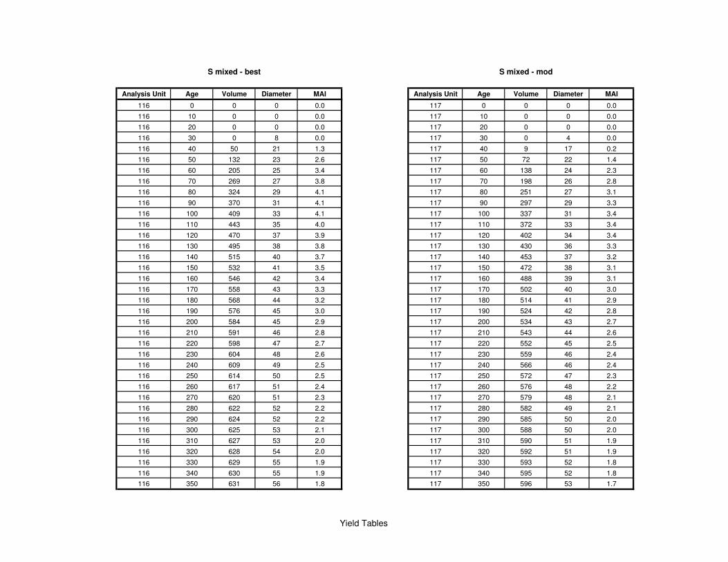
S mixed - best S mixed - mod
Analysis Unit Age Volume Diameter MAI Analysis Unit Age Volume Diameter MAI
116 0 0 0 0.0 117 0 0 0 0.0
116 10 0 0 0.0 117 10 0 0 0.0
116 20 0 0 0.0 117 20 0 0 0.0
116 30 0 8 0.0 117 30 0 4 0.0
116 40 50 21 1.3 117 40 9 17 0.2
116 50 132 23 2.6 117 50 72 22 1.4
116 60 205 25 3.4 117 60 138 24 2.3
116 70 269 27 3.8 117 70 198 26 2.8
116 80 324 29 4.1 117 80 251 27 3.1
116 90 370 31 4.1 117 90 297 29 3.3
116 100 409 33 4.1 117 100 337 31 3.4
116 110 443 35 4.0 117 110 372 33 3.4
116 120 470 37 3.9 117 120 402 34 3.4
116 130 495 38 3.8 117 130 430 36 3.3
116 140 515 40 3.7 117 140 453 37 3.2
116 150 532 41 3.5 117 150 472 38 3.1
116 160 546 42 3.4 117 160 488 39 3.1
116 170 558 43 3.3 117 170 502 40 3.0
116 180 568 44 3.2 117 180 514 41 2.9
116 190 576 45 3.0 117 190 524 42 2.8
116 200 584 45 2.9 117 200 534 43 2.7
116 210 591 46 2.8 117 210 543 44 2.6
116 220 598 47 2.7 117 220 552 45 2.5
116 230 604 48 2.6 117 230 559 46 2.4
116 240 609 49 2.5 117 240 566 46 2.4
116 250 614 50 2.5 117 250 572 47 2.3
116 260 617 51 2.4 117 260 576 48 2.2
116 270 620 51 2.3 117 270 579 48 2.1
116 280 622 52 2.2 117 280 582 49 2.1
116 290 624 52 2.2 117 290 585 50 2.0
116 300 625 53 2.1 117 300 588 50 2.0
116 310 627 53 2.0 117 310 590 51 1.9
116 320 628 54 2.0 117 320 592 51 1.9
116 330 629 55 1.9 117 330 593 52 1.8
116 340 630 55 1.9 117 340 595 52 1.8
116 350 631 56 1.8 117 350 596 53 1.7
Yield Tables

Pine - best Pine - best
Analysis Unit Age Volume Diameter MAI Analysis Unit Age Volume Diameter MAI
118 0 0 0 0.0 119 0 0 0 0.0
118 10 0 0 0.0 119 10 0 0 0.0
118 20 0 0 0.0 119 20 0 1 0.0
118 30 0 0 0.0 119 30 55 16 1.8
118 40 0 7 0.0 119 40 123 18 3.1
118 50 10 17 0.2 119 50 181 20 3.6
118 60 48 21 0.8 119 60 231 21 3.9
118 70 96 23 1.4 119 70 275 23 3.9
118 80 142 24 1.8 119 80 313 24 3.9
118 90 185 26 2.1 119 90 347 26 3.9
118 100 223 28 2.2 119 100 377 27 3.8
118 110 256 29 2.3 119 110 404 28 3.7
118 120 286 31 2.4 119 120 429 30 3.6
118 130 315 32 2.4 119 130 452 31 3.5
118 140 340 33 2.4 119 140 467 32 3.3
118 150 362 35 2.4 119 150 479 33 3.2
118 160 381 36 2.4 119 160 488 33 3.1
118 170 398 37 2.3 119 170 493 34 2.9
118 180 414 37 2.3 119 180 495 34 2.8
118 190 428 38 2.3 119 190 494 35 2.6
118 200 441 39 2.2 119 200 496 35 2.5
118 210 453 40 2.2 119 210 500 35 2.4
118 220 464 41 2.1 119 220 503 36 2.3
118 230 475 42 2.1 119 230 506 36 2.2
118 240 485 43 2.0 119 240 509 37 2.1
118 250 494 44 2.0 119 250 512 37 2.0
118 260 499 44 1.9 119 260 514 38 2.0
118 270 503 45 1.9 119 270 517 38 1.9
118 280 507 45 1.8 119 280 518 38 1.9
118 290 511 46 1.8 119 290 520 38 1.8
118 300 515 46 1.7 119 300 522 39 1.7
118 310 518 47 1.7 119 310 523 39 1.7
118 320 521 47 1.6 119 320 525 39 1.6
118 330 523 48 1.6 119 330 526 40 1.6
118 340 526 49 1.5 119 340 527 40 1.6
118 350 528 49 1.5 119 350 528 40 1.5
Yield Tables

Pine - mod+ Pine - mod
Analysis Unit Age Volume Diameter MAI Analysis Unit Age Volume Diameter MAI
120 0 0 0 0.0 121 0 0 0 0.0
120 10 0 0 0.0 121 10 0 0 0.0
120 20 0 1 0.0 121 20 0 2 0.0
120 30 33 16 1.1 121 30 7 10 0.2
120 40 95 17 2.4 121 40 54 16 1.4
120 50 151 19 3.0 121 50 100 17 2.0
120 60 199 20 3.3 121 60 142 19 2.4
120 70 242 21 3.5 121 70 179 20 2.6
120 80 279 23 3.5 121 80 212 21 2.7
120 90 313 24 3.5 121 90 242 22 2.7
120 100 343 25 3.4 121 100 270 23 2.7
120 110 370 26 3.4 121 110 295 25 2.7
120 120 396 28 3.3 121 120 318 26 2.7
120 130 420 29 3.2 121 130 340 27 2.6
120 140 435 30 3.1 121 140 354 28 2.5
120 150 448 31 3.0 121 150 366 28 2.4
120 160 457 31 2.9 121 160 375 29 2.3
120 170 462 32 2.7 121 170 381 30 2.2
120 180 465 32 2.6 121 180 383 30 2.1
120 190 463 33 2.4 121 190 383 31 2.0
120 200 466 33 2.3 121 200 386 31 1.9
120 210 470 34 2.2 121 210 389 32 1.9
120 220 473 34 2.2 121 220 392 32 1.8
120 230 476 34 2.1 121 230 396 33 1.7
120 240 479 35 2.0 121 240 399 33 1.7
120 250 483 35 1.9 121 250 402 34 1.6
120 260 485 36 1.9 121 260 404 34 1.6
120 270 487 36 1.8 121 270 406 34 1.5
120 280 489 36 1.7 121 280 407 34 1.5
120 290 491 36 1.7 121 290 409 35 1.4
120 300 492 37 1.6 121 300 410 35 1.4
120 310 494 37 1.6 121 310 412 35 1.3
120 320 495 37 1.5 121 320 413 35 1.3
120 330 496 38 1.5 121 330 414 36 1.3
120 340 497 38 1.5 121 340 415 36 1.2
120 350 498 38 1.4 121 350 416 36 1.2
Yield Tables

Pine - poorest Decid - all
Analysis Unit Age Volume Diameter MAI Analysis Unit Age Volume Diameter MAI
122 0 0 0 0.0 123 0 0 0 0.0
122 10 0 0 0.0 123 10 0 0 0.0
122 20 0 2 0.0 123 20 0 1 0.0
122 30 0 2 0.0 123 30 4 8 0.1
122 40 27 15 0.7 123 40 19 12 0.5
122 50 67 17 1.3 123 50 36 18 0.7
122 60 106 18 1.8 123 60 53 20 0.9
122 70 141 19 2.0 123 70 69 22 1.0
122 80 172 20 2.2 123 80 83 24 1.0
122 90 202 21 2.2 123 90 94 26 1.0
122 100 229 22 2.3 123 100 104 27 1.0
122 110 254 23 2.3 123 110 112 29 1.0
122 120 277 24 2.3 123 120 118 31 1.0
122 130 299 25 2.3 123 130 124 32 1.0
122 140 314 26 2.2 123 140 129 33 0.9
122 150 326 26 2.2 123 150 134 34 0.9
122 160 335 27 2.1 123 160 136 35 0.9
122 170 341 27 2.0 123 170 138 35 0.8
122 180 344 28 1.9 123 180 140 36 0.8
122 190 343 28 1.8 123 190 142 36 0.7
122 200 347 29 1.7 123 200 143 36 0.7
122 210 350 29 1.7 123 210 145 37 0.7
122 220 353 30 1.6 123 220 146 37 0.7
122 230 357 30 1.6 123 230 148 38 0.6
122 240 360 31 1.5 123 240 149 38 0.6
122 250 363 31 1.5 123 250 150 38 0.6
122 260 365 32 1.4 123 260 151 38 0.6
122 270 367 32 1.4 123 270 151 39 0.6
122 280 369 32 1.3 123 280 151 39 0.5
122 290 370 33 1.3 123 290 152 39 0.5
122 300 372 33 1.2 123 300 152 39 0.5
122 310 373 33 1.2 123 310 152 39 0.5
122 320 374 33 1.2 123 320 152 39 0.5
122 330 375 34 1.1 123 330 152 39 0.5
122 340 376 34 1.1 123 340 152 40 0.4
122 350 377 34 1.1 123 350 153 40 0.4
Yield Tables

CFLB Coniferous CFLB Deciduous
Analysis Unit Age Volume Diameter MAI Analysis Unit Age Volume Diameter MAI
801 0 0 0 0.0 802 0 0 0 0.0
801 10 0 0 0.0 802 10 0 0 0.0
801 20 0 0 0.0 802 20 0 2 0.0
801 30 3 3 0.1 802 30 5 12 0.2
801 40 15 10 0.4 802 40 23 16 0.6
801 50 38 17 0.8 802 50 44 19 0.9
801 60 69 21 1.2 802 60 63 21 1.1
801 70 103 22 1.5 802 70 80 23 1.1
801 80 136 24 1.7 802 80 95 25 1.2
801 90 166 25 1.8 802 90 107 27 1.2
801 100 193 27 1.9 802 100 118 29 1.2
801 110 217 28 2.0 802 110 126 30 1.1
801 120 238 29 2.0 802 120 133 32 1.1
801 130 259 31 2.0 802 130 139 34 1.1
801 140 278 32 2.0 802 140 144 35 1.0
801 150 294 33 2.0 802 150 149 36 1.0
801 160 309 34 1.9 802 160 152 37 1.0
801 170 322 35 1.9 802 170 155 37 0.9
801 180 333 36 1.9 802 180 157 37 0.9
801 190 343 36 1.8 802 190 159 38 0.8
801 200 353 37 1.8 802 200 160 38 0.8
801 210 363 38 1.7 802 210 162 39 0.8
801 220 372 39 1.7 802 220 164 39 0.7
801 230 381 40 1.7 802 230 165 39 0.7
801 240 389 41 1.6 802 240 167 40 0.7
801 250 397 42 1.6 802 250 168 40 0.7
801 260 400 42 1.5 802 260 169 40 0.7
801 270 403 43 1.5 802 270 169 40 0.6
801 280 405 43 1.4 802 280 169 41 0.6
801 290 408 44 1.4 802 290 169 41 0.6
801 300 410 44 1.4 802 300 170 41 0.6
801 310 412 44 1.3 802 310 170 41 0.5
801 320 414 45 1.3 802 320 170 41 0.5
801 330 416 45 1.3 802 330 170 41 0.5
801 340 417 46 1.2 802 340 170 41 0.5
801 350 418 46 1.2 802 350 170 41 0.5
Yield Tables

Golden TSA TSR4 Data Package
APPENDIX B. MANAGED STANDS (TIPSY) YIELD TABLES <insert tables after this page>
July 18, 2008 1

Lw, Fd (dry) - best Lw, Fd (dry) - mod
Analysis Unit Age Volume Diameter MAI Analysis Unit Age Volume Diameter MAI
201 0 0 0 0.0 202 0 0 0 0.0
201 10 0 0 0.0 202 10 0 0 0.0
201 20 3 14 0.2 202 20 0 0 0.0
201 30 82 22 2.7 202 30 6 16 0.2
201 40 204 27 5.1 202 40 55 21 1.4
201 50 304 31 6.1 202 50 125 24 2.5
201 60 381 34 6.4 202 60 192 27 3.2
201 70 439 37 6.3 202 70 249 29 3.6
201 80 474 39 5.9 202 80 294 31 3.7
201 90 495 41 5.5 202 90 330 33 3.7
201 100 517 42 5.2 202 100 360 34 3.6
201 110 514 42 4.7 202 110 386 35 3.5
201 120 512 42 4.3 202 120 408 36 3.4
201 130 509 42 3.9 202 130 425 37 3.3
201 140 506 42 3.6 202 140 438 38 3.1
201 150 503 42 3.4 202 150 449 38 3.0
201 160 501 42 3.1 202 160 456 39 2.9
201 170 498 42 2.9 202 170 464 39 2.7
201 180 495 42 2.8 202 180 470 40 2.6
201 190 493 42 2.6 202 190 475 40 2.5
201 200 490 42 2.5 202 200 479 41 2.4
201 210 487 42 2.3 202 210 482 41 2.3
201 220 484 42 2.2 202 220 484 41 2.2
201 230 482 42 2.1 202 230 486 41 2.1
201 240 479 42 2.0 202 240 488 41 2.0
201 250 476 42 1.9 202 250 489 42 2.0
201 260 474 42 1.8 202 260 489 42 1.9
201 270 471 42 1.7 202 270 487 42 1.8
201 280 468 42 1.7 202 280 484 42 1.7
201 290 465 42 1.6 202 290 481 42 1.7
201 300 463 42 1.5 202 300 478 42 1.6
201 310 460 42 1.5 202 310 475 42 1.5
201 320 457 42 1.4 202 320 473 42 1.5
201 330 454 42 1.4 202 330 470 42 1.4
201 340 452 42 1.3 202 340 467 42 1.4
201 350 449 42 1.3 202 350 464 42 1.3
Yield Tables

Lw, Fd (wet) - best Lw, Fd (wet) - mod
Analysis Unit Age Volume Diameter MAI Analysis Unit Age Volume Diameter MAI
204 0 0 0 0.0 205 0 0 0 0.0
204 10 0 0 0.0 205 10 0 0 0.0
204 20 1 13 0.1 205 20 0 0 0.0
204 30 57 21 1.9 205 30 4 16 0.1
204 40 182 26 4.6 205 40 51 21 1.3
204 50 300 31 6.0 205 50 134 25 2.7
204 60 382 35 6.4 205 60 213 28 3.6
204 70 449 38 6.4 205 70 283 31 4.0
204 80 496 41 6.2 205 80 338 33 4.2
204 90 529 42 5.9 205 90 382 35 4.2
204 100 561 44 5.6 205 100 419 37 4.2
204 110 558 44 5.1 205 110 451 38 4.1
204 120 555 44 4.6 205 120 476 40 4.0
204 130 552 44 4.2 205 130 495 41 3.8
204 140 549 44 3.9 205 140 511 42 3.7
204 150 547 44 3.6 205 150 525 43 3.5
204 160 544 44 3.4 205 160 537 43 3.4
204 170 541 44 3.2 205 170 548 44 3.2
204 180 538 44 3.0 205 180 556 44 3.1
204 190 535 44 2.8 205 190 563 45 3.0
204 200 532 44 2.7 205 200 568 45 2.8
204 210 529 44 2.5 205 210 573 46 2.7
204 220 526 44 2.4 205 220 577 46 2.6
204 230 523 44 2.3 205 230 580 46 2.5
204 240 520 44 2.2 205 240 576 46 2.4
204 250 517 44 2.1 205 250 573 46 2.3
204 260 514 44 2.0 205 260 570 46 2.2
204 270 511 44 1.9 205 270 566 46 2.1
204 280 508 44 1.8 205 280 563 46 2.0
204 290 505 44 1.7 205 290 560 46 1.9
204 300 502 44 1.7 205 300 557 46 1.9
204 310 499 44 1.6 205 310 553 46 1.8
204 320 496 44 1.6 205 320 550 46 1.7
204 330 493 44 1.5 205 330 547 46 1.7
204 340 490 44 1.4 205 340 543 46 1.6
204 350 487 44 1.4 205 350 540 46 1.5
Yield Tables

Lw, Fd (wet) - poorest Cw - best
Analysis Unit Age Volume Diameter MAI Analysis Unit Age Volume Diameter MAI
206 0 0 0 0.0 207 0 0 0 0.0
206 10 0 0 0.0 207 10 0 0 0.0
206 20 0 0 0.0 207 20 0 0 0.0
206 30 1 13 0.0 207 30 3 15 0.1
206 40 16 18 0.4 207 40 55 21 1.4
206 50 55 21 1.1 207 50 152 25 3.0
206 60 104 23 1.7 207 60 251 29 4.2
206 70 152 25 2.2 207 70 333 33 4.8
206 80 191 27 2.4 207 80 403 36 5.0
206 90 225 28 2.5 207 90 463 38 5.1
206 100 253 30 2.5 207 100 515 40 5.2
206 110 278 31 2.5 207 110 556 42 5.1
206 120 298 32 2.5 207 120 592 44 4.9
206 130 315 33 2.4 207 130 628 45 4.8
206 140 331 33 2.4 207 140 658 47 4.7
206 150 344 34 2.3 207 150 683 48 4.6
206 160 356 35 2.2 207 160 703 49 4.4
206 170 366 35 2.2 207 170 722 50 4.2
206 180 375 36 2.1 207 180 738 50 4.1
206 190 383 36 2.0 207 190 752 51 4.0
206 200 389 37 1.9 207 200 764 52 3.8
206 210 394 37 1.9 207 210 776 52 3.7
206 220 399 37 1.8 207 220 771 52 3.5
206 230 402 37 1.7 207 230 767 52 3.3
206 240 405 38 1.7 207 240 763 52 3.2
206 250 407 38 1.6 207 250 758 52 3.0
206 260 410 38 1.6 207 260 754 52 2.9
206 270 411 38 1.5 207 270 750 52 2.8
206 280 413 39 1.5 207 280 745 52 2.7
206 290 416 39 1.4 207 290 741 52 2.6
206 300 413 39 1.4 207 300 737 52 2.5
206 310 411 39 1.3 207 310 732 52 2.4
206 320 408 39 1.3 207 320 728 52 2.3
206 330 406 39 1.2 207 330 724 52 2.2
206 340 403 39 1.2 207 340 719 52 2.1
206 350 401 39 1.1 207 350 715 52 2.0
Yield Tables

Cw - mod Cw - poorest
Analysis Unit Age Volume Diameter MAI Analysis Unit Age Volume Diameter MAI
208 0 0 0 0.0 209 0 0 0 0.0
208 10 0 0 0.0 209 10 0 0 0.0
208 20 0 0 0.0 209 20 0 0 0.0
208 30 0 0 0.0 209 30 0 0 0.0
208 40 8 17 0.2 209 40 1 14 0.0
208 50 54 21 1.1 209 50 15 18 0.3
208 60 130 25 2.2 209 60 57 21 1.0
208 70 204 28 2.9 209 70 114 24 1.6
208 80 276 30 3.5 209 80 169 27 2.1
208 90 333 33 3.7 209 90 221 29 2.5
208 100 386 35 3.9 209 100 270 30 2.7
208 110 432 37 3.9 209 110 311 32 2.8
208 120 473 39 3.9 209 120 346 34 2.9
208 130 507 40 3.9 209 130 374 35 2.9
208 140 536 42 3.8 209 140 399 36 2.9
208 150 560 43 3.7 209 150 420 37 2.8
208 160 587 44 3.7 209 160 439 38 2.7
208 170 611 45 3.6 209 170 453 39 2.7
208 180 631 46 3.5 209 180 467 39 2.6
208 190 647 47 3.4 209 190 478 40 2.5
208 200 661 47 3.3 209 200 491 41 2.5
208 210 673 48 3.2 209 210 501 41 2.4
208 220 684 49 3.1 209 220 511 42 2.3
208 230 694 49 3.0 209 230 518 42 2.3
208 240 704 50 2.9 209 240 523 43 2.2
208 250 713 50 2.9 209 250 527 43 2.1
208 260 720 51 2.8 209 260 531 44 2.0
208 270 726 51 2.7 209 270 534 44 2.0
208 280 732 51 2.6 209 280 537 44 1.9
208 290 737 52 2.5 209 290 539 44 1.9
208 300 732 52 2.4 209 300 536 44 1.8
208 310 728 52 2.3 209 310 533 44 1.7
208 320 724 52 2.3 209 320 530 44 1.7
208 330 720 52 2.2 209 330 527 44 1.6
208 340 715 52 2.1 209 340 523 44 1.5
208 350 711 52 2.0 209 350 520 44 1.5
Yield Tables

Hw - best Hw - mod
Analysis Unit Age Volume Diameter MAI Analysis Unit Age Volume Diameter MAI
210 0 0 0 0.0 211 0 0 0 0.0
210 10 0 0 0.0 211 10 0 0 0.0
210 20 0 0 0.0 211 20 0 0 0.0
210 30 2 15 0.1 211 30 0 0 0.0
210 40 55 21 1.4 211 40 5 16 0.1
210 50 153 26 3.1 211 50 41 20 0.8
210 60 249 29 4.2 211 60 110 24 1.8
210 70 336 33 4.8 211 70 180 27 2.6
210 80 404 35 5.1 211 80 248 29 3.1
210 90 459 38 5.1 211 90 311 32 3.5
210 100 508 40 5.1 211 100 360 34 3.6
210 110 545 41 5.0 211 110 403 36 3.7
210 120 576 43 4.8 211 120 441 37 3.7
210 130 607 44 4.7 211 130 473 38 3.6
210 140 632 45 4.5 211 140 502 40 3.6
210 150 653 46 4.4 211 150 524 41 3.5
210 160 672 47 4.2 211 160 544 42 3.4
210 170 688 48 4.0 211 170 564 43 3.3
210 180 702 48 3.9 211 180 584 44 3.2
210 190 715 49 3.8 211 190 599 44 3.2
210 200 726 50 3.6 211 200 613 45 3.1
210 210 736 50 3.5 211 210 623 46 3.0
210 220 744 51 3.4 211 220 632 46 2.9
210 230 752 51 3.3 211 230 641 47 2.8
210 240 747 51 3.1 211 240 648 47 2.7
210 250 743 51 3.0 211 250 655 47 2.6
210 260 739 51 2.8 211 260 661 48 2.5
210 270 735 51 2.7 211 270 667 48 2.5
210 280 730 51 2.6 211 280 672 49 2.4
210 290 726 51 2.5 211 290 676 49 2.3
210 300 722 51 2.4 211 300 672 49 2.2
210 310 718 51 2.3 211 310 668 49 2.2
210 320 713 51 2.2 211 320 665 49 2.1
210 330 709 51 2.1 211 330 661 49 2.0
210 340 705 51 2.1 211 340 657 49 1.9
210 350 701 51 2.0 211 350 653 49 1.9
Yield Tables

Hw - poorest B, S - best
Analysis Unit Age Volume Diameter MAI Analysis Unit Age Volume Diameter MAI
212 0 0 0 0.0 213 0 0 0 0.0
212 10 0 0 0.0 213 10 0 0 0.0
212 20 0 0 0.0 213 20 0 0 0.0
212 30 0 0 0.0 213 30 19 18 0.6
212 40 0 0 0.0 213 40 115 25 2.9
212 50 3 15 0.1 213 50 223 29 4.5
212 60 21 19 0.4 213 60 323 32 5.4
212 70 60 21 0.9 213 70 391 34 5.6
212 80 108 24 1.4 213 80 435 36 5.4
212 90 156 26 1.7 213 90 465 38 5.2
212 100 200 28 2.0 213 100 485 39 4.9
212 110 242 29 2.2 213 110 493 40 4.5
212 120 280 31 2.3 213 120 496 41 4.1
212 130 311 32 2.4 213 130 498 41 3.8
212 140 341 33 2.4 213 140 500 42 3.6
212 150 365 35 2.4 213 150 499 42 3.3
212 160 388 36 2.4 213 160 497 42 3.1
212 170 407 36 2.4 213 170 496 43 2.9
212 180 424 37 2.4 213 180 493 43 2.7
212 190 439 38 2.3 213 190 490 43 2.6
212 200 452 39 2.3 213 200 488 43 2.4
212 210 463 39 2.2 213 210 485 43 2.3
212 220 473 40 2.2 213 220 482 43 2.2
212 230 484 40 2.1 213 230 479 43 2.1
212 240 494 41 2.1 213 240 477 43 2.0
212 250 503 41 2.0 213 250 474 43 1.9
212 260 511 42 2.0 213 260 471 43 1.8
212 270 519 42 1.9 213 270 469 43 1.7
212 280 524 43 1.9 213 280 466 43 1.7
212 290 528 43 1.8 213 290 463 43 1.6
212 300 525 43 1.8 213 300 461 43 1.5
212 310 522 43 1.7 213 310 458 43 1.5
212 320 519 43 1.6 213 320 455 43 1.4
212 330 516 43 1.6 213 330 452 43 1.4
212 340 512 43 1.5 213 340 450 43 1.3
212 350 509 43 1.5 213 350 447 43 1.3
Yield Tables

B, S - mod B, S - poorest
Analysis Unit Age Volume Diameter MAI Analysis Unit Age Volume Diameter MAI
214 0 0 0 0.0 215 0 0 0 0.0
214 10 0 0 0.0 215 10 0 0 0.0
214 20 0 0 0.0 215 20 0 0 0.0
214 30 0 13 0.0 215 30 0 0 0.0
214 40 13 17 0.3 215 40 0 13 0.0
214 50 63 22 1.3 215 50 3 16 0.1
214 60 135 26 2.3 215 60 26 19 0.4
214 70 200 28 2.9 215 70 66 22 0.9
214 80 261 30 3.3 215 80 112 25 1.4
214 90 317 32 3.5 215 90 159 27 1.8
214 100 359 33 3.6 215 100 198 28 2.0
214 110 387 35 3.5 215 110 236 29 2.1
214 120 409 36 3.4 215 120 275 31 2.3
214 130 426 36 3.3 215 130 308 32 2.4
214 140 439 37 3.1 215 140 333 33 2.4
214 150 449 38 3.0 215 150 352 34 2.3
214 160 456 38 2.9 215 160 367 34 2.3
214 170 462 39 2.7 215 170 379 35 2.2
214 180 465 39 2.6 215 180 389 35 2.2
214 190 465 40 2.4 215 190 397 36 2.1
214 200 464 40 2.3 215 200 404 36 2.0
214 210 464 40 2.2 215 210 410 37 2.0
214 220 464 40 2.1 215 220 414 37 1.9
214 230 463 41 2.0 215 230 418 37 1.8
214 240 462 41 1.9 215 240 420 38 1.8
214 250 461 41 1.8 215 250 422 38 1.7
214 260 460 41 1.8 215 260 424 38 1.6
214 270 459 41 1.7 215 270 426 38 1.6
214 280 457 41 1.6 215 280 426 39 1.5
214 290 455 41 1.6 215 290 425 39 1.5
214 300 453 41 1.5 215 300 422 39 1.4
214 310 450 41 1.5 215 310 420 39 1.4
214 320 447 41 1.4 215 320 417 39 1.3
214 330 445 41 1.3 215 330 415 39 1.3
214 340 442 41 1.3 215 340 412 39 1.2
214 350 439 41 1.3 215 350 410 39 1.2
Yield Tables

S mixed - best S mixed - mod
Analysis Unit Age Volume Diameter MAI Analysis Unit Age Volume Diameter MAI
216 0 0 0 0.0 217 0 0 0 0.0
216 10 0 0 0.0 217 10 0 0 0.0
216 20 0 0 0.0 217 20 0 0 0.0
216 30 38 20 1.3 217 30 2 15 0.1
216 40 163 26 4.1 217 40 50 21 1.3
216 50 293 31 5.9 217 50 145 25 2.9
216 60 391 35 6.5 217 60 239 29 4.0
216 70 470 38 6.7 217 70 323 32 4.6
216 80 533 41 6.7 217 80 389 35 4.9
216 90 578 43 6.4 217 90 445 37 4.9
216 100 621 45 6.2 217 100 492 39 4.9
216 110 657 47 6.0 217 110 529 41 4.8
216 120 685 48 5.7 217 120 560 43 4.7
216 130 681 48 5.2 217 130 589 44 4.5
216 140 678 48 4.8 217 140 613 45 4.4
216 150 674 48 4.5 217 150 633 46 4.2
216 160 670 48 4.2 217 160 650 47 4.1
216 170 667 48 3.9 217 170 665 48 3.9
216 180 663 48 3.7 217 180 678 48 3.8
216 190 660 48 3.5 217 190 689 49 3.6
216 200 656 48 3.3 217 200 699 49 3.5
216 210 652 48 3.1 217 210 707 50 3.4
216 220 649 48 3.0 217 220 714 50 3.2
216 230 645 48 2.8 217 230 710 50 3.1
216 240 641 48 2.7 217 240 706 50 2.9
216 250 638 48 2.6 217 250 702 50 2.8
216 260 634 48 2.4 217 260 698 50 2.7
216 270 630 48 2.3 217 270 694 50 2.6
216 280 627 48 2.2 217 280 690 50 2.5
216 290 623 48 2.1 217 290 686 50 2.4
216 300 619 48 2.1 217 300 682 50 2.3
216 310 616 48 2.0 217 310 678 50 2.2
216 320 612 48 1.9 217 320 674 50 2.1
216 330 609 48 1.8 217 330 670 50 2.0
216 340 605 48 1.8 217 340 666 50 2.0
216 350 601 48 1.7 217 350 662 50 1.9
Yield Tables

S mixed - poorest Pine - best
Analysis Unit Age Volume Diameter MAI Analysis Unit Age Volume Diameter MAI
218 0 0 0 0.0 219 0 0 0 0.0
218 10 0 0 0.0 219 10 0 0 0.0
218 20 0 0 0.0 219 20 13 13 0.7
218 30 0 0 0.0 219 30 108 21 3.6
218 40 2 15 0.1 219 40 213 26 5.3
218 50 23 19 0.5 219 50 298 29 6.0
218 60 79 22 1.3 219 60 363 32 6.1
218 70 147 25 2.1 219 70 410 34 5.9
218 80 210 28 2.6 219 80 448 36 5.6
218 90 270 30 3.0 219 90 471 37 5.2
218 100 320 32 3.2 219 100 485 38 4.9
218 110 364 34 3.3 219 110 490 39 4.5
218 120 401 36 3.3 219 120 494 40 4.1
218 130 434 37 3.3 219 130 496 41 3.8
218 140 462 39 3.3 219 140 501 41 3.6
218 150 487 40 3.2 219 150 498 41 3.3
218 160 507 41 3.2 219 160 495 41 3.1
218 170 525 42 3.1 219 170 493 41 2.9
218 180 542 42 3.0 219 180 490 41 2.7
218 190 560 43 2.9 219 190 487 41 2.6
218 200 575 44 2.9 219 200 485 41 2.4
218 210 587 45 2.8 219 210 482 41 2.3
218 220 596 45 2.7 219 220 479 41 2.2
218 230 604 46 2.6 219 230 477 41 2.1
218 240 611 46 2.5 219 240 474 41 2.0
218 250 617 47 2.5 219 250 471 41 1.9
218 260 623 47 2.4 219 260 468 41 1.8
218 270 628 47 2.3 219 270 466 41 1.7
218 280 633 48 2.3 219 280 463 41 1.7
218 290 638 48 2.2 219 290 460 41 1.6
218 300 634 48 2.1 219 300 458 41 1.5
218 310 631 48 2.0 219 310 455 41 1.5
218 320 627 48 2.0 219 320 452 41 1.4
218 330 623 48 1.9 219 330 450 41 1.4
218 340 619 48 1.8 219 340 447 41 1.3
218 350 616 48 1.8 219 350 444 41 1.3
Yield Tables

Pine - mod+ Pine - mod
Analysis Unit Age Volume Diameter MAI Analysis Unit Age Volume Diameter MAI
220 0 0 0 0.0 221 0 0 0 0.0
220 10 0 0 0.0 221 10 0 0 0.0
220 20 2 0 0.1 221 20 1 0 0.1
220 30 60 18 2.0 221 30 25 16 0.8
220 40 150 23 3.8 221 40 88 20 2.2
220 50 227 26 4.5 221 50 154 23 3.1
220 60 292 29 4.9 221 60 210 26 3.5
220 70 339 31 4.8 221 70 257 28 3.7
220 80 377 33 4.7 221 80 298 30 3.7
220 90 406 34 4.5 221 90 327 31 3.6
220 100 429 35 4.3 221 100 349 32 3.5
220 110 448 36 4.1 221 110 368 33 3.3
220 120 460 37 3.8 221 120 384 34 3.2
220 130 469 38 3.6 221 130 397 34 3.1
220 140 476 38 3.4 221 140 408 35 2.9
220 150 482 39 3.2 221 150 417 35 2.8
220 160 485 39 3.0 221 160 424 36 2.7
220 170 486 40 2.9 221 170 428 36 2.5
220 180 485 40 2.7 221 180 432 37 2.4
220 190 485 40 2.6 221 190 435 37 2.3
220 200 484 40 2.4 221 200 438 37 2.2
220 210 481 40 2.3 221 210 440 37 2.1
220 220 478 40 2.2 221 220 442 38 2.0
220 230 476 40 2.1 221 230 443 38 1.9
220 240 473 40 2.0 221 240 443 38 1.8
220 250 470 40 1.9 221 250 444 38 1.8
220 260 468 40 1.8 221 260 443 38 1.7
220 270 465 40 1.7 221 270 443 38 1.6
220 280 462 40 1.7 221 280 443 39 1.6
220 290 460 40 1.6 221 290 443 39 1.5
220 300 457 40 1.5 221 300 440 39 1.5
220 310 454 40 1.5 221 310 437 39 1.4
220 320 452 40 1.4 221 320 435 39 1.4
220 330 449 40 1.4 221 330 432 39 1.3
220 340 446 40 1.3 221 340 430 39 1.3
220 350 444 40 1.3 221 350 427 39 1.2
Yield Tables

Pine - poorest Decid - all
Analysis Unit Age Volume Diameter MAI Analysis Unit Age Volume Diameter MAI
222 0 0 0 0.0 223 0 0 0 0.0
222 10 0 0 0.0 223 10 0 0 0.0
222 20 0 0 0.0 223 20 0 0 0.0
222 30 9 13 0.3 223 30 26 19 0.9
222 40 44 17 1.1 223 40 126 25 3.2
222 50 96 21 1.9 223 50 232 29 4.6
222 60 144 23 2.4 223 60 326 32 5.4
222 70 184 25 2.6 223 70 389 34 5.6
222 80 218 26 2.7 223 80 431 36 5.4
222 90 246 27 2.7 223 90 463 38 5.1
222 100 271 28 2.7 223 100 482 39 4.8
222 110 291 29 2.6 223 110 490 40 4.5
222 120 306 30 2.6 223 120 495 41 4.1
222 130 319 31 2.5 223 130 499 41 3.8
222 140 328 31 2.3 223 140 501 42 3.6
222 150 337 32 2.2 223 150 501 42 3.3
222 160 343 32 2.1 223 160 502 43 3.1
222 170 350 32 2.1 223 170 499 43 2.9
222 180 355 33 2.0 223 180 496 43 2.8
222 190 360 33 1.9 223 190 493 43 2.6
222 200 364 33 1.8 223 200 491 43 2.5
222 210 367 34 1.7 223 210 488 43 2.3
222 220 369 34 1.7 223 220 485 43 2.2
222 230 371 34 1.6 223 230 482 43 2.1
222 240 372 34 1.6 223 240 480 43 2.0
222 250 374 34 1.5 223 250 477 43 1.9
222 260 374 35 1.4 223 260 474 43 1.8
222 270 375 35 1.4 223 270 472 43 1.7
222 280 376 35 1.3 223 280 469 43 1.7
222 290 376 35 1.3 223 290 466 43 1.6
222 300 374 35 1.2 223 300 463 43 1.5
222 310 371 35 1.2 223 310 461 43 1.5
222 320 369 35 1.2 223 320 458 43 1.4
222 330 367 35 1.1 223 330 455 43 1.4
222 340 365 35 1.1 223 340 452 43 1.3
222 350 363 35 1.0 223 350 450 43 1.3
Yield Tables

Golden TSA TSR4 Data Package
APPENDIX C. EXISTING MANAGED STANDS (TIPSY) YIELD TABLES <insert tables after this page>
July 18, 2008 1

Lw, Fd (dry) Lw, Fd (wet)
Analysis Unit Age Volume Diameter MAI Analysis Unit Age Volume Diameter MAI
501 0 0 0 0.0 502 0 0 0 0.0
501 10 0 0 0.0 502 10 0 0 0.0
501 20 0 0 0.0 502 20 0 0 0.0
501 30 3 15 0.1 502 30 3 15 0.1
501 40 27 19 0.7 502 40 31 19 0.8
501 50 76 22 1.5 502 50 88 22 1.8
501 60 136 24 2.3 502 60 154 25 2.6
501 70 190 27 2.7 502 70 213 28 3.0
501 80 237 29 3.0 502 80 266 30 3.3
501 90 277 30 3.1 502 90 310 32 3.4
501 100 310 32 3.1 502 100 346 33 3.5
501 110 337 33 3.1 502 110 376 35 3.4
501 120 361 34 3.0 502 120 403 36 3.4
501 130 382 35 2.9 502 130 427 37 3.3
501 140 401 36 2.9 502 140 447 38 3.2
501 150 417 37 2.8 502 150 465 39 3.1
501 160 430 38 2.7 502 160 479 40 3.0
501 170 440 38 2.6 502 170 489 40 2.9
501 180 449 39 2.5 502 180 498 41 2.8
501 190 456 39 2.4 502 190 508 42 2.7
501 200 463 40 2.3 502 200 516 42 2.6
501 210 469 40 2.2 502 210 523 42 2.5
501 220 474 40 2.2 502 220 528 43 2.4
501 230 478 41 2.1 502 230 533 43 2.3
501 240 482 41 2.0 502 240 536 43 2.2
501 250 484 41 1.9 502 250 539 44 2.2
501 260 487 42 1.9 502 260 542 44 2.1
501 270 488 42 1.8 502 270 544 44 2.0
501 280 490 42 1.8 502 280 545 45 1.9
501 290 491 42 1.7 502 290 547 45 1.9
501 300 488 42 1.6 502 300 543 45 1.8
501 310 485 42 1.6 502 310 540 45 1.7
501 320 482 42 1.5 502 320 537 45 1.7
501 330 479 42 1.5 502 330 534 45 1.6
501 340 476 42 1.4 502 340 531 45 1.6
501 350 473 42 1.4 502 350 527 45 1.5
Yield Tables

Cw Hw
Analysis Unit Age Volume Diameter MAI Analysis Unit Age Volume Diameter MAI
503 0 0 0 0.0 504 0 0 0 0.0
503 10 0 0 0.0 504 10 0 0 0.0
503 20 0 0 0.0 504 20 0 0 0.0
503 30 1 15 0.0 504 30 0 13 0.0
503 40 38 20 1.0 504 40 10 17 0.3
503 50 123 24 2.5 504 50 72 22 1.4
503 60 215 28 3.6 504 60 153 25 2.6
503 70 294 31 4.2 504 70 231 29 3.3
503 80 367 34 4.6 504 80 297 31 3.7
503 90 431 36 4.8 504 90 359 34 4.0
503 100 485 38 4.9 504 100 414 36 4.1
503 110 530 40 4.8 504 110 462 38 4.2
503 120 566 42 4.7 504 120 503 39 4.2
503 130 604 43 4.6 504 130 536 41 4.1
503 140 640 45 4.6 504 140 564 42 4.0
503 150 671 46 4.5 504 150 596 43 4.0
503 160 692 47 4.3 504 160 625 44 3.9
503 170 711 48 4.2 504 170 650 46 3.8
503 180 728 49 4.0 504 180 670 46 3.7
503 190 744 49 3.9 504 190 685 47 3.6
503 200 758 50 3.8 504 200 699 48 3.5
503 210 771 51 3.7 504 210 711 49 3.4
503 220 782 51 3.6 504 220 723 49 3.3
503 230 791 52 3.4 504 230 733 50 3.2
503 240 800 52 3.3 504 240 744 50 3.1
503 250 807 53 3.2 504 250 752 51 3.0
503 260 813 53 3.1 504 260 759 51 2.9
503 270 818 53 3.0 504 270 765 51 2.8
503 280 823 54 2.9 504 280 771 52 2.8
503 290 827 54 2.9 504 290 775 52 2.7
503 300 822 54 2.7 504 300 771 52 2.6
503 310 817 54 2.6 504 310 766 52 2.5
503 320 813 54 2.5 504 320 762 52 2.4
503 330 808 54 2.4 504 330 757 52 2.3
503 340 803 54 2.4 504 340 753 52 2.2
503 350 798 54 2.3 504 350 748 52 2.1
Yield Tables

B, S S (mixed)
Analysis Unit Age Volume Diameter MAI Analysis Unit Age Volume Diameter MAI
505 0 0 0 0.0 506 0 0 0 0.0
505 10 0 0 0.0 506 10 0 0 0.0
505 20 0 0 0.0 506 20 0 0 0.0
505 30 1 14 0.0 506 30 0 0 0.0
505 40 17 18 0.4 506 40 10 17 0.3
505 50 75 23 1.5 506 50 56 21 1.1
505 60 151 26 2.5 506 60 123 24 2.1
505 70 216 28 3.1 506 70 191 27 2.7
505 80 278 31 3.5 506 80 251 29 3.1
505 90 336 32 3.7 506 90 307 31 3.4
505 100 377 34 3.8 506 100 355 33 3.6
505 110 406 35 3.7 506 110 394 35 3.6
505 120 427 36 3.6 506 120 427 36 3.6
505 130 443 37 3.4 506 130 452 37 3.5
505 140 457 37 3.3 506 140 474 38 3.4
505 150 468 38 3.1 506 150 492 39 3.3
505 160 475 39 3.0 506 160 511 40 3.2
505 170 481 39 2.8 506 170 528 41 3.1
505 180 484 40 2.7 506 180 542 42 3.0
505 190 485 40 2.6 506 190 554 42 2.9
505 200 483 40 2.4 506 200 561 43 2.8
505 210 483 41 2.3 506 210 567 43 2.7
505 220 483 41 2.2 506 220 572 44 2.6
505 230 481 41 2.1 506 230 576 44 2.5
505 240 481 41 2.0 506 240 580 44 2.4
505 250 480 42 1.9 506 250 585 45 2.3
505 260 478 42 1.8 506 260 588 45 2.3
505 270 477 42 1.8 506 270 591 45 2.2
505 280 475 42 1.7 506 280 594 46 2.1
505 290 473 42 1.6 506 290 595 46 2.1
505 300 470 42 1.6 506 300 592 46 2.0
505 310 468 42 1.5 506 310 588 46 1.9
505 320 465 42 1.5 506 320 585 46 1.8
505 330 462 42 1.4 506 330 581 46 1.8
505 340 459 42 1.4 506 340 578 46 1.7
505 350 457 42 1.3 506 350 574 46 1.6
Yield Tables

Pine Decid - all
Analysis Unit Age Volume Diameter MAI Analysis Unit Age Volume Diameter MAI
507 0 0 0 0.0 508 0 0 0 0.0
507 10 0 0 0.0 508 10 0 0 0.0
507 20 1 0 0.1 508 20 1 0 0.1
507 30 16 14 0.5 508 30 23 16 0.8
507 40 62 18 1.6 508 40 107 22 2.7
507 50 119 22 2.4 508 50 197 26 3.9
507 60 171 24 2.9 508 60 272 29 4.5
507 70 214 26 3.1 508 70 344 31 4.9
507 80 251 27 3.1 508 80 395 33 4.9
507 90 286 29 3.2 508 90 425 35 4.7
507 100 313 30 3.1 508 100 447 36 4.5
507 110 333 31 3.0 508 110 467 37 4.2
507 120 349 32 2.9 508 120 482 38 4.0
507 130 363 32 2.8 508 130 493 39 3.8
507 140 375 33 2.7 508 140 498 40 3.6
507 150 386 34 2.6 508 150 499 40 3.3
507 160 396 34 2.5 508 160 500 41 3.1
507 170 404 35 2.4 508 170 501 41 2.9
507 180 411 35 2.3 508 180 502 42 2.8
507 190 416 35 2.2 508 190 502 42 2.6
507 200 420 36 2.1 508 200 501 42 2.5
507 210 423 36 2.0 508 210 500 42 2.4
507 220 426 36 1.9 508 220 498 43 2.3
507 230 428 37 1.9 508 230 496 43 2.2
507 240 430 37 1.8 508 240 494 43 2.1
507 250 431 37 1.7 508 250 492 43 2.0
507 260 433 37 1.7 508 260 490 43 1.9
507 270 434 37 1.6 508 270 487 43 1.8
507 280 435 38 1.6 508 280 484 43 1.7
507 290 435 38 1.5 508 290 481 43 1.7
507 300 433 38 1.4 508 300 478 43 1.6
507 310 430 38 1.4 508 310 475 43 1.5
507 320 428 38 1.3 508 320 473 43 1.5
507 330 425 38 1.3 508 330 470 43 1.4
507 340 423 38 1.2 508 340 467 43 1.4
507 350 420 38 1.2 508 350 464 43 1.3
Yield Tables

Backlog 1 Backlog 2
Analysis Unit Age Volume Diameter MAI Analysis Unit Age Volume Diameter MAI
525 0 0 0 0.0 526 0 0 0 0.0
525 0 0 0 0.0 526 0 0 0 0.0
525 20 0 0 0.0 526 20 0 0 0.0
525 30 0 0 0.0 526 30 0 0 0.0
525 40 0 0 0.0 526 40 0 0 0.0
525 50 6 16 0.1 526 50 1 0 0.0
525 60 27 19 0.5 526 60 12 17 0.2
525 70 68 24 1.0 526 70 44 22 0.6
525 80 120 27 1.5 526 80 94 26 1.2
525 90 170 30 1.9 526 90 148 29 1.6
525 100 212 32 2.1 526 100 193 31 1.9
525 110 250 34 2.3 526 110 235 34 2.1
525 120 283 35 2.4 526 120 270 35 2.3
525 130 311 37 2.4 526 130 300 37 2.3
525 140 333 38 2.4 526 140 323 38 2.3
525 150 352 39 2.3 526 150 344 39 2.3
525 160 370 40 2.3 526 160 362 40 2.3
525 170 385 41 2.3 526 170 378 41 2.2
525 180 398 41 2.2 526 180 390 42 2.2
525 190 409 42 2.2 526 190 400 43 2.1
525 200 417 43 2.1 526 200 409 43 2.0
525 210 424 43 2.0 526 210 417 44 2.0
525 220 431 44 2.0 526 220 423 44 1.9
525 230 437 44 1.9 526 230 428 45 1.9
525 240 441 44 1.8 526 240 433 45 1.8
525 250 445 45 1.8 526 250 436 46 1.7
525 260 448 45 1.7 526 260 439 46 1.7
525 270 451 45 1.7 526 270 442 46 1.6
525 280 453 46 1.6 526 280 444 46 1.6
525 290 455 46 1.6 526 290 446 47 1.5
525 300 457 46 1.5 526 300 447 47 1.5
525 310 457 46 1.5 526 310 448 47 1.4
525 320 455 46 1.4 526 320 448 47 1.4
525 330 452 46 1.4 526 330 446 47 1.4
525 340 449 46 1.3 526 340 443 47 1.3
525 350 447 46 1.3 526 350 440 47 1.3
Yield Tables

Lw, Fd (dry) Lw, Fd (wet)
Analysis Unit Age Volume Diameter MAI Analysis Unit Age Volume Diameter MAI
601 0 0 0 0.0 602 0 0 0 0.0
601 10 0 0 0.0 602 10 0 0 0.0
601 20 0 0 0.0 602 20 0 0 0.0
601 30 3 15 0.1 602 30 1 14 0.0
601 40 37 20 0.9 602 40 27 19 0.7
601 50 98 23 2.0 602 50 95 23 1.9
601 60 163 26 2.7 602 60 172 26 2.9
601 70 219 28 3.1 602 70 243 29 3.5
601 80 266 30 3.3 602 80 302 32 3.8
601 90 305 32 3.4 602 90 351 34 3.9
601 100 335 33 3.4 602 100 392 36 3.9
601 110 360 34 3.3 602 110 429 38 3.9
601 120 384 35 3.2 602 120 459 39 3.8
601 130 402 36 3.1 602 130 485 41 3.7
601 140 417 37 3.0 602 140 508 42 3.6
601 150 430 38 2.9 602 150 526 43 3.5
601 160 438 39 2.7 602 160 541 44 3.4
601 170 446 39 2.6 602 170 555 44 3.3
601 180 453 39 2.5 602 180 567 45 3.2
601 190 459 40 2.4 602 190 578 46 3.0
601 200 464 40 2.3 602 200 587 46 2.9
601 210 468 41 2.2 602 210 594 46 2.8
601 220 471 41 2.1 602 220 601 47 2.7
601 230 474 41 2.1 602 230 606 47 2.6
601 240 475 41 2.0 602 240 611 48 2.5
601 250 477 42 1.9 602 250 615 48 2.5
601 260 478 42 1.8 602 260 619 48 2.4
601 270 479 42 1.8 602 270 622 48 2.3
601 280 480 42 1.7 602 280 618 48 2.2
601 290 480 42 1.7 602 290 615 48 2.1
601 300 477 42 1.6 602 300 611 48 2.0
601 310 474 42 1.5 602 310 607 48 2.0
601 320 471 42 1.5 602 320 604 48 1.9
601 330 468 42 1.4 602 330 600 48 1.8
601 340 466 42 1.4 602 340 597 48 1.8
601 350 463 42 1.3 602 350 593 48 1.7
Yield Tables

Cw Hw
Analysis Unit Age Volume Diameter MAI Analysis Unit Age Volume Diameter MAI
603 0 0 0 0.0 604 0 0 0 0.0
603 10 0 0 0.0 604 10 0 0 0.0
603 20 0 0 0.0 604 20 0 0 0.0
603 30 1 14 0.0 604 30 0 0 0.0
603 40 35 20 0.9 604 40 13 17 0.3
603 50 123 24 2.5 604 50 71 22 1.4
603 60 216 28 3.6 604 60 153 25 2.6
603 70 304 31 4.3 604 70 232 29 3.3
603 80 372 34 4.7 604 80 304 32 3.8
603 90 433 37 4.8 604 90 361 34 4.0
603 100 487 39 4.9 604 100 414 36 4.1
603 110 532 41 4.8 604 110 459 38 4.2
603 120 567 43 4.7 604 120 499 40 4.2
603 130 601 44 4.6 604 130 532 41 4.1
603 140 633 45 4.5 604 140 560 43 4.0
603 150 660 47 4.4 604 150 587 44 3.9
603 160 683 48 4.3 604 160 613 45 3.8
603 170 702 48 4.1 604 170 636 46 3.7
603 180 718 49 4.0 604 180 653 47 3.6
603 190 734 50 3.9 604 190 669 48 3.5
603 200 748 51 3.7 604 200 682 48 3.4
603 210 759 51 3.6 604 210 695 49 3.3
603 220 770 52 3.5 604 220 706 50 3.2
603 230 780 52 3.4 604 230 716 50 3.1
603 240 788 53 3.3 604 240 725 50 3.0
603 250 795 53 3.2 604 250 733 51 2.9
603 260 790 53 3.0 604 260 740 51 2.8
603 270 786 53 2.9 604 270 745 52 2.8
603 280 781 53 2.8 604 280 751 52 2.7
603 290 777 53 2.7 604 290 755 52 2.6
603 300 772 53 2.6 604 300 751 52 2.5
603 310 767 53 2.5 604 310 746 52 2.4
603 320 763 53 2.4 604 320 742 52 2.3
603 330 758 53 2.3 604 330 738 52 2.2
603 340 754 53 2.2 604 340 733 52 2.2
603 350 749 53 2.1 604 350 729 52 2.1
Yield Tables

B, S S (mixed)
Analysis Unit Age Volume Diameter MAI Analysis Unit Age Volume Diameter MAI
605 0 0 0 0.0 606 0 0 0 0.0
605 10 0 0 0.0 606 10 0 0 0.0
605 20 0 0 0.0 606 20 0 0 0.0
605 30 1 14 0.0 606 30 11 14 0.4
605 40 25 19 0.6 606 40 54 18 1.4
605 50 93 24 1.9 606 50 110 21 2.2
605 60 174 27 2.9 606 60 162 24 2.7
605 70 244 30 3.5 606 70 206 26 2.9
605 80 314 32 3.9 606 80 243 27 3.0
605 90 364 34 4.0 606 90 276 29 3.1
605 100 398 35 4.0 606 100 303 30 3.0
605 110 422 36 3.8 606 110 322 31 2.9
605 120 441 37 3.7 606 120 337 32 2.8
605 130 457 38 3.5 606 130 350 32 2.7
605 140 467 39 3.3 606 140 362 33 2.6
605 150 475 39 3.2 606 150 371 34 2.5
605 160 477 40 3.0 606 160 380 34 2.4
605 170 477 40 2.8 606 170 387 35 2.3
605 180 478 41 2.7 606 180 392 35 2.2
605 190 478 41 2.5 606 190 396 35 2.1
605 200 477 41 2.4 606 200 400 36 2.0
605 210 477 41 2.3 606 210 402 36 1.9
605 220 476 42 2.2 606 220 405 36 1.8
605 230 475 42 2.1 606 230 407 36 1.8
605 240 474 42 2.0 606 240 408 37 1.7
605 250 473 42 1.9 606 250 409 37 1.6
605 260 470 42 1.8 606 260 411 37 1.6
605 270 468 42 1.7 606 270 411 37 1.5
605 280 466 42 1.7 606 280 412 37 1.5
605 290 463 42 1.6 606 290 412 37 1.4
605 300 461 42 1.5 606 300 410 37 1.4
605 310 458 42 1.5 606 310 407 37 1.3
605 320 455 42 1.4 606 320 405 37 1.3
605 330 452 42 1.4 606 330 402 37 1.2
605 340 450 42 1.3 606 340 400 37 1.2
605 350 447 42 1.3 606 350 398 37 1.1
Yield Tables

Pine Decid - all
Analysis Unit Age Volume Diameter MAI Analysis Unit Age Volume Diameter MAI
607 0 0 0 0.0 608 0 0 0 0.0
607 10 0 0 0.0 608 10 0 0 0.0
607 20 0 0 0.0 608 20 0 0 0.0
607 30 16 15 0.5 608 30 12 17 0.4
607 40 69 19 1.7 608 40 86 23 2.2
607 50 130 22 2.6 608 50 183 27 3.7
607 60 184 25 3.1 608 60 270 30 4.5
607 70 229 27 3.3 608 70 343 33 4.9
607 80 268 28 3.4 608 80 390 34 4.9
607 90 301 30 3.3 608 90 424 36 4.7
607 100 324 31 3.2 608 100 450 37 4.5
607 110 343 32 3.1 608 110 468 38 4.3
607 120 359 33 3.0 608 120 479 39 4.0
607 130 372 33 2.9 608 130 483 40 3.7
607 140 384 34 2.7 608 140 488 40 3.5
607 150 394 35 2.6 608 150 491 41 3.3
607 160 402 35 2.5 608 160 494 41 3.1
607 170 409 36 2.4 608 170 494 42 2.9
607 180 414 36 2.3 608 180 494 42 2.7
607 190 417 36 2.2 608 190 493 42 2.6
607 200 420 37 2.1 608 200 491 42 2.5
607 210 422 37 2.0 608 210 489 42 2.3
607 220 425 37 1.9 608 220 486 42 2.2
607 230 426 37 1.9 608 230 483 42 2.1
607 240 427 37 1.8 608 240 480 42 2.0
607 250 428 38 1.7 608 250 478 42 1.9
607 260 429 38 1.7 608 260 475 42 1.8
607 270 430 38 1.6 608 270 472 42 1.7
607 280 430 38 1.5 608 280 470 42 1.7
607 290 431 38 1.5 608 290 467 42 1.6
607 300 428 38 1.4 608 300 464 42 1.5
607 310 426 38 1.4 608 310 461 42 1.5
607 320 423 38 1.3 608 320 459 42 1.4
607 330 420 38 1.3 608 330 456 42 1.4
607 340 418 38 1.2 608 340 453 42 1.3
607 350 415 38 1.2 608 350 450 42 1.3
Yield Tables

Backlog 1 Backlog 2
Analysis Unit Age Volume Diameter MAI Analysis Unit Age Volume Diameter MAI
625 0 0 0 0.0 626 0 0 0 0.0
625 10 0 0 0.0 626 10 0 0 0.0
625 20 0 0 0.0 626 20 0 0 0.0
625 30 2 15 0.1 626 30 4 16 0.1
625 40 36 20 0.9 626 40 54 21 1.4
625 50 109 24 2.2 626 50 141 25 2.8
625 60 188 27 3.1 626 60 222 28 3.7
625 70 258 30 3.7 626 70 299 31 4.3
625 80 320 32 4.0 626 80 355 33 4.4
625 90 365 34 4.1 626 90 397 35 4.4
625 100 399 35 4.0 626 100 430 36 4.3
625 110 427 36 3.9 626 110 457 38 4.2
625 120 450 37 3.8 626 120 477 39 4.0
625 130 468 38 3.6 626 130 494 40 3.8
625 140 482 39 3.4 626 140 505 40 3.6
625 150 494 40 3.3 626 150 514 41 3.4
625 160 502 41 3.1 626 160 521 42 3.3
625 170 508 41 3.0 626 170 527 42 3.1
625 180 513 42 2.9 626 180 532 43 3.0
625 190 518 42 2.7 626 190 536 43 2.8
625 200 522 42 2.6 626 200 538 43 2.7
625 210 525 43 2.5 626 210 541 44 2.6
625 220 527 43 2.4 626 220 543 44 2.5
625 230 529 43 2.3 626 230 544 44 2.4
625 240 530 43 2.2 626 240 545 44 2.3
625 250 531 44 2.1 626 250 545 44 2.2
625 260 531 44 2.0 626 260 545 45 2.1
625 270 532 44 2.0 626 270 542 45 2.0
625 280 532 44 1.9 626 280 539 45 1.9
625 290 531 44 1.8 626 290 536 45 1.8
625 300 528 44 1.8 626 300 533 45 1.8
625 310 525 44 1.7 626 310 529 45 1.7
625 320 522 44 1.6 626 320 526 45 1.6
625 330 519 44 1.6 626 330 523 45 1.6
625 340 516 44 1.5 626 340 520 45 1.5
625 350 513 44 1.5 626 350 517 45 1.5
Yield Tables