THE ECONOMICS OF TIMBER SUPPLY: AN ANALYTICAL SYNTHESIS …

NATURAL RESOURCE MODELINGVolume 8, Number 3, Summer 1994

THE ECONOMICS OF TIMBERSUPPLY: AN ANALYTICAL SYNTHESIS

OF MODELING APPROACHES

DAVID N. WEARU.S.D.A. Forest ServicePost Office Box 12254

Research Triangle Park, NC 27709

PETER J. PARKSDepartment of Agricultural Economics and Marketing

Cook College, Rutgers UniversityPost Office Box 231

New Brunswick, NJ 08903-0231

ABSTRACT. The joint supply of timber and other servicesfrom forest environments plays a central role in most forestland debates. This paper defines a general conceptual modelof timber supply that provides the context for discussing bothindividual harvest choice and aggregate supply models. Whilethe structure and breadth of these models has developedconsiderably over the last twenty years, unresolved issuesremain. Supply formulations that account for the qualityand vintage distribution of forest capital will be necessaryfor improving medium- and long-run forecasts. This will beespecially important for examining the potential impacts ofstructural changes in forest production and timber markets.In addition, consistent aggregation of individual owners tototal supply will be required to address changing forest landownership patterns.

KEY WORDS: Timber supply, forest policy, supply mod-els.

Introduction. This paper examines methods for modeling timbersupply. The paper begins by presenting an analytical framework, thenuses this framework to organize existing literature. The framework isdifferent than that used in earlier surveys of this subject (e.g., Adamsand Haynes [1980], Alig, Lewis, and Morris [1984], Binkley [1987]) andpresents new insights. As the types of questions examined with timbersupply models have changed, it is reasonable to ask whether the existingmodels can still be used to help answer them. This review of existing

Revised April, 1994.

Copyright 01994 Rocky Mountain Mathematics Consortium

199

200 D.N. WEAR AND P.J. PARKS

models defines research frontiers and identifies opportunities for furtherresearch.

Timber supply defines an important contemporary issue for resourceanalysis. For example, in the Pacific Northwestern United Statesregulations have recently been implemented under the EndangeredSpecies Act to protect the Northern Spotted Owl (5%~ occidentaliscaurina) from extinction. These regulations have led to dramaticreductions in wood production from National Forests in the PacificNorthwest, a region that has historically produced roughly one third ofthe total softwood timber in the United States. Contracting woodproduction has had substantial impact on derivative wood productmanufacturing and employment, especially in this region, but also inother wood-producing regions.

Shifts in domestic markets also have implications for the internationaltrade of wood products and the location of wood processing employ-ment, both between Canada and the U.S. and between North America,Europe, and the Pacific Rim. Unraveling complex effects (both do-mestic and international) has been the subject of considerable researcheffort; this effort has produced methodological tools that will be invalu-able for analyzing the impacts of new policies and programs.

Although trade-offs between wildlife habitat protection and timberproduction are an important contemporary issue, this is hardly the onlyissue that could be used to motivate a review of timber supply modeling.Analyzing the nature and extent of forests is required to evaluate topicssuch as global warming and the role of trees in sequestering carbon,harvesting in tropical forests, the structure of resource concessions, thedirect trade of forest products and the derivative trade of environmentalhazard. While these specific questions are beyond the scope of thispaper, their answers in part must derive from an understanding of thestructure of timber supply.

Conceptual frarnework. Timber supply models summarize theproduction behavior of forest managers in a market setting. Modelingtimber supply requires information on the biological/physical produc-tion possibilities of timber growing and inventory adjustment, as wellas information on the objectives of forest landowners. When sector-level timber supplies are to be examined, heterogeneous forest land

ECONOMICS OF TIMBER SUPPLY 201

and owners with heterogeneous objectives must be aggregated.

This section provides an analytical framework for classifying anddiscussing existing models and defining where gaps between theory andempirical application exist. A timber production function is introducedfirst to define production possibilities. The section then describes howindividual decision models may be aggregated in various ways to definesector-level timber supply.

Timber production function. Underlying any study of productionis a production function which translates inputs into outputs. Fortimber supply, the inputs should include the age of the forest, a, thelevel of forest management effort, E, and the quality of the land, q.Merchantable timber volume per unit area, V, is given by the yieldfunction:

(1) V = ~(a, E; q).

The marginal physical products of age and management effort arepositive and decreasing in the relevant ranges of age and effort. Theseproperties can be summarized (Binkley [1987]) as:

Forest harvesting decisions. Provided that the forest manager’sobjective function can be specified, then the forest yield function canbe used to define if and when a forest stand would be harvested. Forexample, consider a manager who faces prices p for timber and w formanagement effort (e.g., effort used to reforest the land after harvest).When the land is maintained indefinitely in forest use, the managerwill maximize profit by selecting harvest ages a and levels of effort Eto optimize:

(3) rF = max{a, -E} F{pv(a, E; q)esTa - wE}eeTa’jj=o

= max{a, E}pv(a, E; q)evra - WE

l--~--m .

D.N. WEAR AND P.J. PARKS

The optimum profit obtained, Tag, is the present net value for an in-finite sequence of identical harvest ages. This formulation provides avaluation for forest land of quality q when there are no trees presentat the beginning of the manager’s planning horizon. The manager’sproblem can easily be modified to allow for the benefit provided by ex-isting timber inventories; however, when profit from timber enterpriseis the only argument in the objective function (cf. Hartman [1976]) thesolution for optimum age (a*) is unaffected by the manager’s startinginventory of timber. With this definition of profit, the manager recog-nizes that there is an opportunity cost to holding old trees rather thanfaster-growing young trees, and that this opportunity cost influencesthe harvest timing decision.’

As long as the manager’s optimum timber profits are positive andgreater than the value of land in alternative uses, then the manager’ssolution to (3) will identify profit-maximizing harvest dates, harvestvolumes, and levels of regeneration effort. The optimum harvest ageis obtained where the marginal benefits from delaying the harvest arejust equal to the marginal opportunity costs of the delay:

p%(a*,E;9) = & bu(a* > E; 4) - WEI

Marginal benefits attributable to postponing harvest, MBD(a, E; q),shown on the left-hand side of equation (4), are derived from thevalue of an additional year’s growth. Marginal opportunity costs frompostponing harvest, MOC(a, E; q), shown on the right-hand side ofequation (4), are the discounted opportunity costs of future harvestrevenues.

When forest management decisions are guided by utility rather thanprofit maximization, the forest management problem may be more com-plex than that described by equations (3) and (4). For example, non-priced amenity services may be included in the manager’s objectivefunction, or forest-level constraints may bind on local decisions. How-ever, even when these questions are addressed in the manager’s prob-lem, similar decision rules are obtained (i.e., where marginal benefitsand costs of delaying harvest are balanced).2 For subsequent discussionhere, we posit that a decision rule exists which defines the economi-cally optimal harvest age for each forest owner and quality class. Ifwe define the manager’s current expectation of future market prices as


pe, the manager’s optimum harvest age under these expectations, 6, isgiven by

qP,Pe;q) = a : MBDe(a, E; q) = MOC”(a, E; 4).

The manager’s optimum harvest age, 6, depends on current marketsignals (p) and market expectations (p”). This optimum age is notnecessarily the same as that given by equation (4), and will likely varyover time as price expectations are revised.3 Equation (4) is a long-runsolution where all elements of pe are equal to p.

Aggregate supply. Consider the aggregate supply provided by thismanager from an ownership of size L when land quality* varies from4- to 4’9 and the age of standing timber varies from a- to a+. Theforest can be described by the density function, c,h(q,a) which givesthe relative frequency of land of quality q that is occupied by trees ofage class a. Given the manager’s harvesting rules, which are derivedin equation (5), current timber supply can be defined by integratingacross forest area with age greater than d for each quality class

(6) SfR c L ‘+JJ a+ 4a, E Ma, 4) da & = dp,pe; @(a, d).q- B

The notation SSR indicates short-run (current period) supply, whichdepends on current and future prices of products, input costs, and theexisting age and quality attributes of the fores&j

The supply is a short-run quantity because (i) it allows for seculartrends in prices (i.e. all elements of pe are not necessarily equal to p)and (ii) harvest quantity is constrained in the short run by L4(a, q), thequantity and quality of forest land and the age-distribution of currentinventory. Brazee and Mendelsohn [1990] develop a similar supplyfunction that allows for optimal transition to long-run conditions whenprice is sensitive to aggregate output. The current inventory of timbervolume is:

9+ a+I, = LJJ v(a, E; qM(a, q&d+

q- a-


In the long-run, the manager allocates land among age classes accord-ing to equation (4) with l/a* (p, q) of the land in each age class6 Themanager allocates land among forest and nonforest uses by identifyingthe optimum land use margin (see below). The long-run equilibrium,consistent with the forester’s definition of a sustained yield forest, ischaracterized by a uniform age-class distribution between the age ofzero and a* (p, q), the optimal long-run rotation age:

(8) StLR = Ls

‘+ da, E; q)$q(q)q-

--$--$q = gdwNFL>

The function cbq(q) is the marginal distribution of land quality thatcorresponds to the joint distribution $(a, q). In the manager’s long-runsupply equation (equation (8)), the joint distribution of age and landquality, 4(a, q), has been replaced by the product of the marginal distri-bution for land quality, a,(q), and the uniform density for a regulatedforest on quality class q managed at age u*(p, q) (i.e., l/a*(p, q)). Themanager’s optimum age is identified when marginal benefits of delayequal the marginal opportunity costs of delay (i.e., equation (4)). Theland quality margin between forest and nonforest uses is given by

q(p,pNF) = q+ : n*yq+) = 7r*yq+),

where pNF and reNF are the prices and profits, respectively, associatedwith the highest-valued nonforest land use. The lowest land qualitythat can provide nonnegative profits to forestry is given by x*F(q-) =0 .

To this point, the manager has supplied only a single representativeproduct. This assumption may hold in areas where, for example,sawtimber is the exclusive product of timber production. It may nothold, however, where both sawtimber and pulpwood or other timberproducts are produced (e.g., the Southeast). Multiple products maybe aggregated into a total product formulation only in the specialcase of product separability. To account for 1 multiple products( i = 1,2,... , I), the manager defines a production function for eachproduct,

(10) Vi = ~?(a, E; q),


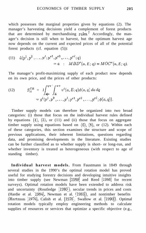
which possesses the marginal properties given by equations (2). Themanager’s harvesting decisions yield a complement of forest productsthat are determined by merchandising rules.7 Accordingly, the man-ager’s decision is still when to harvest, but the optimum harvest agenow depends on the current and expected prices of all of the potentialforest products (cf. equation (5)):

(11) iL(p1,p2 ,‘.’ ,p1;pe1,pe2 ,‘.. ,p”‘;q)

=u : MBD”(a, E; q) = MOC”(a, E; q).

The manager’s profit-maximizing supply of each product now dependson its own price, and the prices of other products:

(12) s$” = L q+ss

a+vi(a,E;q)O(a,q)dadqq- &

=gi(p1,p2 ,... ,p’;pe1,pe2 ,... ,#;4(a,q)).

Timber supply models can therefore be organized into two broadcategories: (i) those that focus on the individual harvest rules definedby equations (4), (5), or (11) and (ii) those that focus on aggregatetimber supply using equations based on (6), (8), or (12). Within eachof these categories, this section examines the structure and scope ofprevious applications, their inherent limitations, questions regardingdata, and promising developments in the literature. Existing studiescan be further classified as to whether supply is short- or long-run, andwhether inventory is treated as heterogeneous (with respect to age ofstanding timber).

Individual harvest models. From Faustmann in 1849 throughseveral studies in the 1990’s the optimal rotation model has proveduseful for studying forestry decisions and developing intuitive insightsinto timber supply (see Newman [1988] and Reed [1986] for recentsurveys). Optimal rotation models have been extended to address riskand uncertainty (Routledge [1980]), secular trends in prices and costs(Hardie et al. [1984], Newman et al. [1985]), and nontimber benefits(Hartman [1976], Calish et al. [1976], Swallow et al. [1990]). Optimalrotation models typically employ engineering methods to calculatesupplies of resources or services that optimize a specific objective (e.g.,


discounted net cash flow). However, these normative models are notthe exclusive approach to studying individual harvest choices.

Harvesting behavior has also been examined using positive, discretechoice models. These econometric models have proved useful forexamining the influence of various site and forest-owner characteristicson harvest decisions in either a utility or a profit-maximizing framework(e.g., Binkley [1981]). D iscrete choice models have also been applied toforest investment (regeneration) decisions (e.g., Royer [1987]).

Both normative (engineering) and positive (econometric) harvestdecision models may be useful for examining timber harvesting. Thissection discusses the structure of both types of models. Aggregation ofindividual owner models is presented in the next section.

Normative harvest models. F’austmann’s model [1849] of harvesttiming for a perpetual series of rotations on land that is initially bare(equation (3)) ha s b een extensively used to develop more recent insightsinto timber supply. While the bare land problem is the intellectualantecedent to virtually all normative harvest models, it represents ahighly restrictive case. In contrast to this standard model, prices andcosts have not been constant through time and are rarely anticipatedwith certainty. One can, however, generalize the decision model definedin equation (3) for the case where timber prices vary through time;prices are typically allowed to vary during a transition period beforethey reach steady-state values, p,. This defines a dynamic optimizationproblem where the decision variables are a sequence of rotations whichcan be of different lengths (cf. equation (3)):

( 1 3 ) 7rF

+ max{a,}psv(u,)ewTa~ - wEe-'.~" tj

1 - e-rU8 3=1 .

In this formulation, timber price p(t) is a function of calendar time.The manager’s problern is divided into two components: one describinga transition period through which prices are variable and anotherdescribing an anticipated steady state where price is constant. Thesecond component is equivalent to the bare land model and it possesses

ECONOMICS OF TIMBER SUPPLY

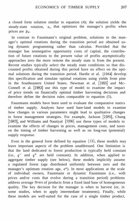
a closed form solution similar to equation (4); the solution yields thesteady-state rotation, a,, that optimizes the manager’s profits whenprices are ps.

In contrast to Faustmann’s original problem, solutions to the man-ager’s optimal rotations during the transition period are obtained us-ing dynamic programming rather than calculus. Provided that themanager has nonnegative opportunity costs of capital, the contribu-tion of future rotations to the present value of profits asymptoticallyapproaches zero the more remote the steady state is from the present.Recent studies typically select the steady state conditions so that dis-counted profits obtained during this period have no effect on the opti-mal solutions during the transition period. Hardie et al. 119841 developthis specification and simulate optimal rotations using yields from pinein the Southeastern United States. Newman et al. [1985] and Mc-Connell et al. [1983] use this type of model to examine the impactof price trends on financially optimal timber harvesting decisions andtherefore define the decision rules comparable to equation (5).

Faustmann models have been used to evaluate the comparative staticsof timber supply. Analysts have used bare-land models to examinehow changes in various parameters might lead to qualitative changesin forest management strategies. For example, Jackson [1980], Chang[1983], and Williams and Nautiyal [1990] use these types of models toexamine the effects of changes in prices, management costs, and taxeson the timing of timber harvesting as well as on long-run (potential)supply response.

Even in the general form defined by equation (13), these models mayleave important aspects of the problem unaddressed. One limitation isthat the land dedicated to forest production is typically held constant(i.e., q- and q+ are held constant). In addition, when applied toaggregate timber supply (see below), these models implicitly assumea regulated forest (age distributed uniformly between zero and themanager’s optimum rotation age, a*). In most applications at the scaleof individual owners, Faustmann or dynamic Faustmann (i.e., withprices and/or costs that evolve during a transition period) problemsaddress average flows of products from a fixed land base of homogeneousquality. The key decision for the manager is when to harvest (or, insome studies, when to apply intermediate treatments). Finally, whilethese models are well-suited for the case of a single timber product,


failure to meet conditions required for product separability have madethem less useful for analyzing multiproduct situations.

Therefore, while normative harvest models have been useful fordeveloping insights into the structure of supply, used alone, theyare inherently limited as sector-level supply models. However, whenindividual harvest models are aggregated in ways which account forinteractions between production and price, timber harvest models haveprovided an important foundation for supply analysis. Aggregatemodels will be discussed after positive harvest models.

Positive harvest models. Positive models of harvest choice areempirical applications of the decision rules defined by equation (5).Existing applications at the level of the individual forest manager lookdirectly at the implied marginal conditions between harvesting anddelaying harvest on a particular stand for a particular owner. Studiesconstructed at this level of analysis generally assume that the managermaximizes utility, ZL. Utility is most often a function of wealth (whichincludes income provided by harvest of merchantable timber products)and other attributes (e.g., amenities from the standing forest, bequestvalues of standing timber capital) that may enter the manager’s utilitydirectly. Utility for forest management choice i for stand j usuallytakes the form:

(14) uij = fi(Zj, Xcj).

Utility depends on a vector of stand attributes, zj, such as age,management intensity, land quality, as well as owner attributes, xj,such as education and income.

The manager’s optimum harvest decision in this context depends onthe marginal utility of delaying harvest and the marginal opportunitycost (in terms of foregone current utility) from delaying harvest. Ac-cordingly, positive harvest choice models are estimated using discretechoice methods (e.g. logit and probit models) fit to cross sectional ob-servations of harvest and delay choices and landowner and forest qualitycharacteristics (e.g. Binkley [1981] and Dennis [1989]). In addition, thesimultaneous decision regarding how much to harvest has also been in-vestigated using Tobit formulations (Dennis [1990], Kuuluvainen andSal0 [1991]).


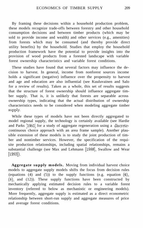
By framing these decisions within a household production problem,these models recognize trade-offs between forestry and other householdconsumption decisions and between timber products (which may besold to provide income and wealth) and other services (e.g., amenities)from forests which may be consumed (and thereby provide directutility benefits) by the household. Studies that employ the householdproduction framework have the potential to provide insights into theprovision of wood products from a forested landscape with variableforest ownership characteristics and variable forest conditions.

These studies have found that several factors may influence the de-cision to harvest. In general, income from nonforest sources incomeholds a significant (negative) influence over the propensity to harvestand age and education are also influential (see Kuuluvainen and Salofor a review of results). Taken as a whole, this set of results suggeststhat the structure of forest ownership should influence aggregate tim-ber supply. That is, it is unlikely that forests are separable acrossownership types, indicating that the actual distribution of ownershipcharacteristics needs to be considered when modeling aggregate timbersupply.

While these types of models have not been directly aggregated tomodel regional supply, the technology is certainly available (see Hardieand Parks [1991] for a study of aggregate regeneration using a discrete-continuous choice approach with an area frame sample). Another plau-sible extension of these models is to study the joint production of tim-ber and nontimber services. However, the specification of the requi-site production relationships, including spatial relationships, remains asubstantial challenge (see Max and Lehmann [1988], Swallow and Wear[1993]).

Aggregate supply models. Moving from individual harvest choicemodels to aggregate supply models shifts the focus from decision rules(equations (4) and (5)) to the supply functions (e.g. equation (6),(8), and (12)). These supply functions have been constructed bymechanically applying estimated decision rules to a variable forestinventory (referred to below as mechanistic or engineering models).More frequently, aggregate supply is estimated as a direct econometricrelationship between short-run supply and aggregate measures of priceand average forest conditions.


As they have been applied to date, aggregate supply models are gen-erally not pure applications of econometrics or mathematical program-ming. Rather they are generally hybrid approaches which utilize vari-ous combinations of econometrics and optimization on both the demandand supply sides of wood products markets.

Engineering supply models. Individual timber harvest modelsmay be applied across heterogeneous timber inventory and land qualityto define regional timber supply. This approach requires some assump-tions regarding the overall structure of the market (perfect competitionis usually assumed) and information on the existing timber inventory.8Another key component is the time-structure of the models: some fo-cus on the eventual long-run supply response of a timber sector; othersfocus the optimal transition of the sector to a long-run state given an-ticipated changes in exogenous factors. Both approaches are normativein that they project behavior based, not on historical actions, but onthe solution of profit maximization problems.

Long run engineering models have been constructed directly fromnormative individual harvest models. These engineering models aresolved for the optimal harvest date and harvest quantity for each forestquality class. Optimization results can then be translated into annualproduct flows by assuming that, in the long run, the age distributionof each managed forest class will be uniform between the ages of zeroand the optimal rotation age. Accordingly, the total area divided bythe rotation age defines the portion of area harvested and the totalquantity of product harvested each year in the steady state. The long-run supply function can then be formed by solving this problem overa range of timber prices. The approach can be summarized with thefollowing algorithm:

1. The forest land base is arranged into various categories basedon the quality of the forest site and/or its distance from demandcenters. Li(q) is the area of land in quality class q and location class

2. A timber price, p, is specified

3. Equation (3) is solved for the optimal harvest age, a*. Thecorresponding harvest volume per acre, w(u*, E; q), and profit, rTF(q),


are calculated for each quality/location class.

4. If rTF(q) > 0 then this quality of forest is suitable for timbermanagement.

5. By assuming that the age-distribution is approximately uniformbetween the ages of 0 and a* in the long run, the average annual timberoutput from each suitable class is defined as

Sjhd = 4a*,E;qPj(dla*.

6. Total supply for a specific price is then defined as the sum of suppliesfrom quality classes q- to q+ and location classes 1 to J:

q=q+ J

S(P) = z: t: %(q)q=q- j=l

where

-%(d =Sj(p,q) i f x:(q) > 0 , a n do

otherwise.

7. Construct the long-run timber supply for a region by repeatingsteps 2 through 6 for a range of timber prices.

The advantage of this method is that it defines a production potentialconsistent with a capital theoretic analysis of timberlands. Lands pro-vide timber only when timber management generates positive profit.The approach is also relatively simple to implement and it is a usefultool for examining the long-run impacts of changes in both market con-ditions and biophysical production relationships (the u(a, E; q)). Be-cause of its relatively simple structure, the approach can accommodatemore detail than is usually possible with large scale optimization oreconometric models of s~pply.~

The usefulness of the approach is limited by its long-run focus.Supply in the short and medium runs may be highly variable inresponse to market fluctuations and the most obvious criticism of thisapproach is that the long run is typically so far off in forestry asto be irrelevant to the supply problems at hand. This is especiallyproblematic when considering cases where the age class distributionsof the forest capital is skewed from the long-run uniform condition


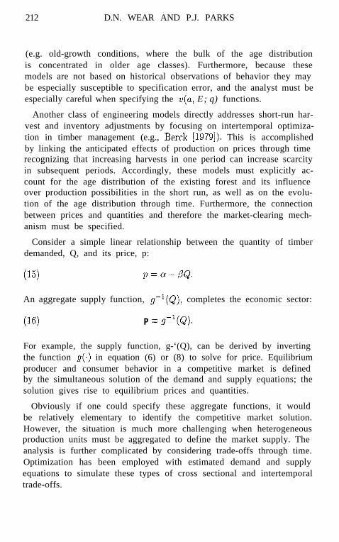
(e.g. old-growth conditions, where the bulk of the age distributionis concentrated in older age classes). Furthermore, because thesemodels are not based on historical observations of behavior they maybe especially susceptible to specification error, and the analyst must beespecially careful when specifying the ~(a, E; q) functions.

Another class of engineering models directly addresses short-run har-vest and inventory adjustments by focusing on intertemporal optimiza-tion in timber management (e.g., Berck [1979]). This is accomplishedby linking the anticipated effects of production on prices through timerecognizing that increasing harvests in one period can increase scarcityin subsequent periods. Accordingly, these models must explicitly ac-count for the age distribution of the existing forest and its influenceover production possibilities in the short run, as well as on the evolu-tion of the age distribution through time. Furthermore, the connectionbetween prices and quantities and therefore the market-clearing mech-anism must be specified.

Consider a simple linear relationship between the quantity of timberdemanded, Q, and its price, p:

(15) p=a-/3Q.

An aggregate supply function, g-l(Q), completes the economic sector:

(16) P = g-l(Q).

For example, the supply function, g-‘(Q), can be derived by invertingthe function g(.) in equation (6) or (8) to solve for price. Equilibriumproducer and consumer behavior in a competitive market is definedby the simultaneous solution of the demand and supply equations; thesolution gives rise to equilibrium prices and quantities.

Obviously if one could specify these aggregate functions, it wouldbe relatively elementary to identify the competitive market solution.However, the situation is much more challenging when heterogeneousproduction units must be aggregated to define the market supply. Theanalysis is further complicated by considering trade-offs through time.Optimization has been employed with estimated demand and supplyequations to simulate these types of cross sectional and intertemporaltrade-offs.


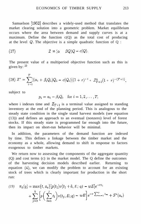
Samuelson [1952] describes a widely-used method that translates themarket clearing solution into a geometric problem. Market equilibriumoccurs where the area between demand and supply curves is at amaximum. Define the function c(Q) as the total cost of producingat the level Q. The objective is a simple quadratic function of Q :

(17) 2 = (a - PQ)Q - c(Q).

The present value of a multiperiod objective function such as this isgiven by: lo

(18) z* = f)(% + Pi&J&i - c(Qi)](l + T)-~ + Z;+,(I + r)++l),i = l

subject topi=ai-BiQi fori=1,2 ,..., T,

where i indexes time and Zr+i is a terminal value assigned to standinginventory at the end of the planning period. This is analogous to thesteady state condition in the single stand harvest models (see equation(13)) and defines an approach to an eventual (nonzero) level of foreststocks. If this steady state is programmed far enough into the future,then its impact on short-run behavior will be minimal.

In addition, the parameters of the demand function are indexedby time. This defines a linkage between the timber market and theeconomy as a whole, allowing demand to shift in response to factorsexogenous to timber markets.

We return now to assessing the components of the aggregate quantity(Q) and cost terms (c) in the market model. The Q define the outcomesof the harvesting decision models described earlier. Returning toequation (4), we can modify the problem to account for an existingstock of trees which is clearly important for production in the shortrun:

(19) nz(q) = max{t, a,}lp(ti)u(ti + Z, E; q) - wE]e-Ttl

+$ [~( $ti)u(lj,E;q) - wE]e-‘C-=l~~ +s*(a8)


where si is the existing age of the stand, q is site quality, and S is thesteady state volume from equation (4). Simulating market behaviorrequires that quantities produced by solving (19) with given prices,generate these prices when evaluated in model (18).

There are various ways to approach the solution of this problem.One is to simply iterate between the market solution (18) and theindividual producer problems (19): define an initial price vector, solve(19) with these prices, solve (18) with the resulting quantities, andthen solve (19) again with the resulting prices. This iteration betweenthe market problem and individual subproblems continues until pricesand quantities converge. This approach has been applied by Sallnasand Eriksson 119891 in their analysis of timber markets in SouthernSweden.

The iterative approach provides a straightforward solution techniqueand an explicit link between harvest decisions and aggregate supply,but may limit the breadth of policy issues which can be addressed.In particular, there are a number of issues that can only be modeledby limiting production in a particular period or constraining decisionsacross a subset of forest owners or a class of forest land. For thesetypes of questions, an alternative formulation of the linkage betweenthe market and individual behavior is required. This requires buildinga large scale optimization model which directly incorporates the standlevel decisions as decision variables in the market objective function.This kind of model accommodates policies which are simulated withconstraint sets. This type of approach is incorporated, for example, inLyon and Sedjo’s [1986] optimal control model of international tradein temperate forest products.

While intertemporal optimization models have the advantage of ad-dressing short- and medium-run market behavior, they still presentthe same kind of specification problems that face long-run engineeringmodels. That is, they require the model to approximate the essentialdecision making mechanisms in the optimization problem. The result-ing sensitivity to specification error demands careful attention to modelcalibration (an area which has not received extensive attention).

The strength of the engineering approach is that (given the abovequalification) the underlying production models are explicitly defined.Accordingly, these models are especially well-suited for studying the


implications of changes in biophysical productivity associated with, forexample, global climate change. In general, these models hold advan-tage for simulating the structure of nonmarginal changes in the timber-producing sector. These would include the effects of productivity shiftsrelated to global climate change.

However, while they hold great advantage for generating hypothesesregarding nonmarginal changes and making detailed forecasts, engi-neering models have no role in testing hypotheses regarding supplybehavior. This is the strength of econometric approaches to modelingtimber supply which is taken up next.

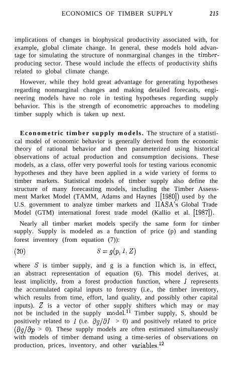
Econometric timber supply models. The structure of a statisti-cal model of economic behavior is generally derived from the economictheory of rational behavior and then parameterized using historicalobservations of actual production and consumption decisions. Thesemodels, as a class, offer very powerful tools for testing various economichypotheses and they have been applied in a wide variety of forms totimber markets. Statistical models of timber supply also define thestructure of many forecasting models, including the Timber Assess-ment Market Model (TAMM, Adams and Haynes [1980]) used by theU.S. government to analyze timber markets and IIASA’s Global TradeModel (GTM) international forest trade model (Kallio et al. [1987]).

Nearly all timber market models specify the same form for timbersupply. Supply is modeled as a function of price (p) and standingforest inventory (from equation (7)):

(20) s = S(P, I, 2)

where S is timber supply, and g is a function which is, in effect,an abstract representation of equation (6). This model derives, atleast implicitly, from a forest production function, where I representsthe accumulated capital inputs to forestry (i.e., the timber inventory,which results from time, effort, land quality, and possibly other capitalinputs). 2 is a vector of other supply shifters which may or maynot be included in the supply model.‘l Timber supply, S, should bepositively related to I (i.e. t?g/aI > 0) and positively related to price(as/& > 0). These supply models are often estimated simultaneouslywith models of timber demand using a time-series of observations onproduction, prices, inventory, and other variables.12


While these supply formulations have proved empirically powerful,they are not always explicitly tractable to theories of production be-havior (Binkley [1987], Wear [1991]). For example, these models cannotdistinguish the effects of various structures of forest capital (e.g., differ-ent age distributions comprising the same timber volume) which mightbe represented by the aggregate inventory variable. When the age-distribution and species composition of the forest capital is relativelyconstant this may not be a problem. However, the misspecification maybe serious when these qualities vary substantially. For example, an in-ventory skewed towards newly planted forests is qualitatively distinctfrom the same level of inventory represented by old growth forests ora bimodal age distribution. Because of these limitations, which derivefrom the lack of explicit links to the production technology and the dy-namics of forest capital, these models are limited in scope to the studyof short-run supply responses.

One reason for the lack of detail in aggregate supply models is thesmall number of observations available in time series. An alternativeapproach is to look at production in cross-section (where more detaileddata are available) and to impute the temporal dynamics. One ap-proach, taken by Wear and Newman [1991] is to examine output andinvestment decisions simultaneously using a restricted profit function.This formulation allows sawtimber and pulpwood supply to be assessedin a theoretically consistent framework and allows direct testing of var-ious homogeneity and separability assumptions.

Within this context, pulpwood and sawtimber supply are examinedas joint products while land, growing stock, and regeneration inputare considered nonseparable inputs to timber production. With landand growing stocks considered quasi-fixed, short-run supply has thefollowing form (cf. equation (12)):

(21) si = f(PS,PP,W,I,L)

where Si is the supply of product i (either sawtimber or pulpwood),ps is the price of sawtimber, pp is the price of pulpwood, w is the costof regeneration, I is the level of growing stocks of timber, and L is thequantity of land dedicated to timber production. This type of modelaccounts for substitution between timber products by including thedifferent product price variables as well as the impacts of investment


costs on production (i.e. the w variable). In addition, the equationdistinguishes between land and growing stock components of inventoryso that stock:land ratios can impact supply. However, it assumes thatgrowing stocks of various vintages are separable.

Because short-run and long-run responses are associated with thesame production function (with and without binding input constraintsrespectively), long-run response can be imputed from the envelope ofshort-run behavior (cf. Lau [1976]). Le Chatelier’s Rule requires thatlong-run elasticities be greater than short-run elasticities.13

While this model defines the long-run elasticities of supply impliedby the envelope of short-run decisions, the actual transition betweenshort and long run remains unaddressed. To date, econometric modelshave not directly studied this important medium-run (e.g., ten years)phenomenon. This is clearly an important issue, especially given therelatively long life of capital invested in wood product manufacture, tobe addressed by forthcoming timber supply work as analysts considerthe implications of shifts in forest inventories.

Summary and conclusions. This paper has reviewed variousmethods for modeling the supply of timber. The conceptual modelshows that the question is complicated by substitution both intertem-porally and between vintages of capital. It is this essential role of timein production that sets forestry apart from most other applications ofresource economics. Accounting for the resulting age structure of for-est capital remains as one of the most substantial challenges for timbersupply modelers.

Applications are divided into two categories: (i) those that focus onindividual timber harvest rules and (ii) those that focus on aggregatetimber supply. Research has been extensive in both areas, though per-haps the greatest opportunity for future advances is at the interface be-tween individual harvest rules and their aggregate supply consequences.Aggregate models built through theoretically consistent aggregation ofindividual choice models hold great promise for improving knowledgeand forecasts of timber supply.

Individual harvest models have the benefit of allowing extensive detailin the modeling of forestry decisions. Given the complexity of forestconditions and often the complexity of management objectives, the


detail allowed by these models may provide important insights into thestructure of timber supply.

Normative harvest choice models, following in the Faustmann tradi-tion, continue to stimulate interest and provide the framework for muchof the forest economics literature. Their specifications have become in-creasingly complex to reflect, among other things, joint production ofmultiple marketed and nonmarket products. This complexity raisesconcerns about specification errors. However, the primary purpose ofthese models is neither to forecast nor to test hypotheses. Rather itis to develop insights and perhaps to define hypotheses for subsequents tudy .

Empirical forms of these decision models-referred to in this paperas “positive harvest models”-have seen extensive development overthe last five years. These models allow the investigator to proposeand test for the relationships between various factors and individualtimber production decisions. While several interesting results havebeen obtained, they can generally be summarized as follows: thecharacteristics of forest owners have a significant bearing on forestmanagement decisions. Accordingly, the structure of ownership mattersin determining timber supply and changes in forest ownership can havesignificant aggregate impacts.

However, accounting for ownership structure is rarely found in aggre-gate timber supply models. To date, the detail allowed by individualchoice models has not been accommodated into large scale applicationsbecause of data limitations. This is especially true for econometric sup-ply models that have been the basis for most policy analysis within theU.S. and around the globe. Some recent efforts suggest, however, thatadditional information may be developed from the analysis of cross-sectional datasets.

The lack of detail in the specification of econometric models of tim-ber supply limits the scope of policies that can be analyzed. In par-ticular long-run responses cannot be derived directly from presentapproaches-though long-term forecasting can be accomplished withad hoc adjustments to inventory. An important first step in improvingtimber supply projections is to link long-term inventory adjustmentmodels to economic decision models. The considerable challenge for


timber supply modelers is to address the long-run structure of timbersupply in theoretically consistent terms.

Extensive production detail and long-run adjustments may be ac-commodated in mechanistic market models. These approaches havebeen recently enhanced by improved computer technologies that allowfor more efficient solution algorithms and larger data storage capacity.Enormous mathematical programming formulations of timber marketsmay therefore be accommodated. These models provide expansions ofFaustmann-style forest management models to the market as a whole.

These types of models are especially useful for forecasting the effectsof structural changes in timber markets (i.e., changes that are non-marginal or without historical precedent). For example, they may beuseful for exploring shifts in timber production technologies from evento uneven aged management systems (Haight [1994]). Other examplesinclude environmental factors such as global climate change or acidrain and policy factors such as large-scale changes in the availabilityof national forest timber. However, credible models must be basedon a foundation of assumptions derived from empirical analysis. So,while these types of models hold considerable promise for improvingthe precision of forecasts, this promise is inextricably tied to the qualityof information provided by econometric models.

ENDNOTES

1. The first correct capital theoretic analysis of forest production is generallyattributed to Faustmann [1849]. The problem has been rediscovered or extendedby several other researchers. Lofgren [1983] p rovides a discussion of the early historyof this problem and Newman [1988] provides a survey of more than eighty relatedpapers in English-language journals.models by Reed [1986].

In addition, see the review of harvesting

2. Although decision rules can become quite complex, especially when spatialjuxtaposition of stands is included (e.g., Swallow and Wear [1993]), they generallyreduce to this simple structure. When existing stands and nontimber benefits thatincrease with stand age are considered, corner solutions involving immediate harvestand permanent preservation are also possible (e.g., Hartman [1976]).

3. At an aggregate level expectations may be endogenously formed through aninventory management problem (Lewandrowski, Wohlgenant, and Grennes [1994]).Endogenous prices are considered in more detail below, when the demand fortimber is introduced. In addition, price expectations may be sensitive to changesin the regulatory environment surrounding forest management. Anticipation ofrestrictions and uncertain property rights would necessarily work against long-terminvestments in timber production.


4. In the long run, both the upper and lower limits of the quality class distributionof land allocated to forest use can change. These changes result from long-rundynamic adjustments of land inputs in response to changes in relative forest andnonforest benefits (see below).

5. The optimum age a is given in equation (5) above. The function g(.) onlyimplicitly depends on prices via a(~,$; q). Equation (6) presents the function asexplicit to facilitate comparison with the abundant applications of this equation inthe literature.

6. Equation (4) applies here because p equals pe in the long run.

7. The use of merchandising rules defines a kind of product separability. It impliesthat forest managers affect product mix only through harvest timing decisions, butnot by substituting between products at a given harvest age. While this may seemrestrictive, it appears reasonable, given the very large premium paid for sawtimberover pulpwood-i.e., it is generally unreasonable to assume that sawtimber-sizematerial would be sold as pulpwood.

8. Market structure is an interesting but infrequently addressed topic in foresteconomics. Early studies of market power include Mead’s [1966] study of lumberoroduction in the U.S. Pacific Northwest, and Lowrv and Winfrey’s /1974] analysisof the pulp and paper industry. A collection of studies by Johansson and Liifgren[1985] examines various hypotheses regarding market power in the wood productsindustries in Sweden. Most recently, Murray [1992] tests for market power in bothpulpwood and sawtimber markets in the U.S. (Murray also reviews previous workin this area).

9. This type of analysis was initially developed by Vaux [1954]. Hyde [1980] usedlong-run models to examine various scenarios for the Pacific Northwest region ofthe United States. Robinson et al. [1978] h ave also used these models to examinelong-run supply in the U.S. South.

10. For a good discussion of the mathematical programming approach to sectormodeling in general, see Hazel1 and Norton [1986].

11. Binkley [1987] points out that the theoretical justification for the inventoryvariable differs from one application to another. In practice, it may be the onlyvariable available to identify the parameters in the supply and demand equationsystem.

12. There are several examples of this type of econometric model includingJackson [1983] for the state of Montana, Daniels and Hyde [1986] for the stateof North Carolina, Brlnnlund et al. [1985] for Sweden, and Newman [1987] for theU.S. South.

13. We appreciate the efforts of an anonymous reviewer, who pointed this out.Empirical validation of this in a timber supply context is provided in Newman andWear [1993]. In addition, their results lend support to findings from the qualitativechoice models of timber harvesting. That is, they find that ownership characteristicsmatter to aggregate timber supply and that nonindustrial and industrial ownersbehave differently in their pursuit of forest management.


REFERENCES

Adams, D.M. and R.W. Haynes [1980], The 1980 softwood timber assessmentmarket model: Structure, projections and policy simulations, Forest Science Mono-graph 22 64 pp.

Alig, R.J., B.J. Lewis, and P.A. Morris [1984], Aggregate timber supply analyses,United States Department of Agriculture, Forest Service, Rocky Mountain Forestand Range Experiment Station, General Technical Report RM-106, Fort Collins.

Berck, P. [1979], The economics of timber: A renewable resource in the long run,Bell Journal of Economics 10 (2), 447-462.

Binkley, C.S. [1981], Timber supply from nonindustrial forests, Bulletin No. 92,Yale University, School of Forestry and Environmental Studies, New Haven, 97 pp.

Binkley, C.S. (19871, Economic models of timber supply, in The global forestsector: An analytical perspective (Kallio, Dykstra and Binkley, eds.), John Wileyand Sons, New York, 703 pp.

Brlinnlund, R., P.-O. Johansson and K.G. Lafgren [1985], An econometric analysisof aggregate sawtimber and pulpwood supply in Sweden, Forest Science 31, 595-606.

Brazee, R. and R. Mendelsohn [1990], A dynamic model of timber markets, ForestScience 36 (2), 255-264.

Calish, S., R.D. Fight and D.E. Teeguarden [1978], How do nontimber valuesaffect Douglas-fir rotations?, Journal of Forestry 76, 217-221.

Chang, S.J. [1983], Rotation age, management intensity, and the economic factorsof production, Forest Science 29 (2), 267-277.

Daniels, B. and W.F. Hyde [1986], Estimation of supply and demand elasticitiesfor North Carolina timber, Forest Ecology and Management 14, 59-67.

Dennis, D.F. [1989], An economic analysis of harvest behavior: Integrating forestand ownership characteristics, Forest Science 35 (4), 1088-1104.

Dennis, D.G. [1990], A probit analysis of the harvest decision using pooledtime series and cross-sectional data, Journal of Environmental Economics andManagement 18, 176-187.

Faustmann, M. [1849], Calculation of the value which forest land and immaturestands possess for forestry, in Martin Faustmann and the evolution of discountedcash jaw (M. Gane, ed.) [1968], reprinted in English translation, Oxford Institute,Oxford, 27-55.

Haight, R.G. [1994], Technology change and the economics of silvicultural invest-ment, United States Department of Agriculture, Forest Service, Rocky MountainForest and Range Experiment Station, General Technical Report RM-232, FortCollins.

Hardie, I.W., J.N. Daberkow and K.E. McConnell [1984], A timber harvestingmodel with variable rotation lengths, Forest Science 30 (2), 511-523.

Hardie, I.W. and P.J. Parks [1991], Acreage response to cost-sharing in the South,1971-1981: Integrating individual choice and regional acreage response, ForestScience 37 (l), 175-190.

Hartman, R. [1976], The harvest decision when the standing forest has value,Economic Inquiry 14, 52-58.


Hazel& P.B.R. and R.D. Norton [1986], Mathematical programming for economicanalysis in agriculture Macmillan, New York, 502 pp.

Hyde, W.F. [1980], Timber supply, land allocation, and economic eficiency, TheJohns Hopkins University Press, Baltimore, 225 pp.

Jackson, D.H. [1980], The microeconomics of the timber industry, Westview Press,Boulder, 136 pp.

Jackson, D.H. [1983], Sub-regional timber demand analysis: Remarks and anapproach for prediction, Forest Ecology and Management, 5 109-118.

Johansson, P.-O. and K.G. Lb;fgren 119851, The economics offorestry and naturalresources, Basil Blackwell Inc., New York, 292 pp.

Kallio, M., D.P. Dykstra and C.S. Binkley, eds. [1987], The global forest sector:An analytical perspective, John Wiley and Sons, New York.

Kuuluvainen, J. and J. Sale [1991], Timber supply and life cycle harvest ofnonindustrial private forest owners: An empirical analysis of the Finnish case,Forest Science 37 (4), 1011-1029.

Lau, L.J. [1976], A characterization of the normalized restricted profit function,Journal of Economic Theory 12, 131-163.

Lewandrowski, J.K., M.K. Wohlgenant, and T.J. Grennes [1994], Finished prod-ucts inventories and price expectations in the softwood lumber industry, AmericanJournal of Agricultural Economics 76 (l), 83-93.

LGfgren, K.G. [1983], The Faustmann-Ohlin theorem: A historical note, Historyof Political Economy 15 (2), 261-264.

LBfgren, K.G. [1985], Effects on the socially optimal rotation period in forestryof biotechnological improvements of the growth function, Forest Ecology and Man-agement 10 (2), 233-249.

LGfgren, K.G. 119871, Effects of permanent and non-permanent forest means ontimber supply, Silva Fennica 20, 308-311.

Lowry, S.T. and J.C. Winfrey [1974], The kinked cost curve and the dual resourcebase under oligopsony in the pulp and paper industry, Land Economics 50, 185-192.

Lyon, K.S. and R.A. Sedjo [1986], B’tnary search SPOC: An optimal controlversion of ECHO, Forest Science 32 (3), 576-584.

Max, W. and D.E. Lehmann [1988], A behavioral model of timber supply, Journalof Environmental Economics and Management 15, 71-86.

McConnell, D.E., J.N. Daberkow and I.W. Hardie [1983], Planning timber pro-duction with evolving prices and costs, Land Economics 59 (3), 292-299.

Mead, W.J. [1966], Competition and oligopsony in the Douglas-fir lumber indus-try, The University of California Press, Berkeley.

Murray, B.C. [1992], Testing for imperfect competition in spatially differentiatedmarkets: The case of U.S. markets for pulpwood and sawlogs, Ph.D. Dissertation,School of the Environment, Duke University, Durham, NC.

Newman, D.H. [1987], An econometric analysis of the southern softwood stumpagemarket: 1950-1980, Forest Science 33 932-945.


Newman, D.H. [1988], The optimal forest rotation: A discussion and annotatedbibliography, General Technical Report No. SE-48, U.S.D.A. Southeastern ForestExperiment Station, Asheville.

Newman, D.H., C.B. Gilbert and W.F. Hyde [1985], The optimal forest rotationwith evolving prices, Land Economics 61 (4), 347-353.

Newman, D.H. and D.N. Wear [1993], Production economics of private forestry:A comparison of industrial and nonindustrial forest owners, American Journal ofAgricultural Economics 75, 674-684.

Reed, W.J. [1986], Optimal harvesting models in forest management: A survey,Natural Resource Modeling 1 (l), 55-79.

Robinson, V.L., A.A. Montgomery and J.S. Strange [1978], GASPLY: A computermodel for Georgia's future forest, Georgia Forest Research Report 26A, GeorgiaForest Research Council, Macon, 21 pp.

Routledge, R.D. [1980], The efiect of potential catastrophic mortality and otherunpredictable events on forest rotation policy, Forest Science 28 (3), 389-399.

Royer, J.P. [1987], Determination of reforestation behavior among southernlandowners, Forest Science 33, 654-667.

SallnL, 0. and L.O. Eriksson [1989], Management variation and price expec-tations in an intertemporal forest sector model, Natural Resource Modeling 3,385-398.

Samuelson, P.A. [1952], Spatial price equilibrium and linear programming, Amer-ican Economic Review 42, 283-303.

Swallow, S.K., P.J. Parks and D.N. Wear [1990], Policy relevant nonconvezitiesin the production of multiple forest benefits, Journal of Environmental Economicsand Management 19, 264-280.

Swallow, S.K. and D.N. Wear [1993], Spatial interactions in multiple use forestryand substitution and wealth effects for the single stand, Journal of EnvironmentalEconomics and Management 25, 103-120.

Vaux, H.J. [1954], Economics of young growth sugar pine resources, Bulletin No.78, Division of Agricultural Sciences, University of California, Berkeley.

Wear, D.N. [1991], Evaluating technology and policy shifts in the forest sector:Technical issues for analysis, in Proceedings of the 1991 Southern Forest EconomicsWorkshop (S.J. Chang, ed.), Washington.

Wear, D.N. and W.F. Hyde [1992], Distributive issues in forest policy, Journal ofBusiness Administration 21, 297-314.

Wear, D.N. and D.H. Newman [1991], The production structure of forestry: Short-run and long-run results, Forest Science 37 (2), 540-551.

Williams, J.S. and J.C. Nautiyal [1990), The long-run timber supply function,Forest, Science 36 (l), 77-86.

THE ECONOMICS OF TIMBER SUPPLY: AN ANALYTICAL SYNTHESIS …

Documents

Transcript of THE ECONOMICS OF TIMBER SUPPLY: AN ANALYTICAL SYNTHESIS …