
Tilburg University Essays on finance van Toor, Joris · 2017-12-19 · Essays on Finance: Drivers...
221
Tilburg University Essays on finance van Toor, Joris Document version: Publisher's PDF, also known as Version of record Publication date: 2017 Link to publication Citation for published version (APA): van Toor, J. (2017). Essays on finance: Drivers of bank performance and the international cost of equity Tilburg: CentER, Center for Economic Research General rights Copyright and moral rights for the publications made accessible in the public portal are retained by the authors and/or other copyright owners and it is a condition of accessing publications that users recognise and abide by the legal requirements associated with these rights. - Users may download and print one copy of any publication from the public portal for the purpose of private study or research - You may not further distribute the material or use it for any profit-making activity or commercial gain - You may freely distribute the URL identifying the publication in the public portal Take down policy If you believe that this document breaches copyright, please contact us providing details, and we will remove access to the work immediately and investigate your claim. Download date: 13. Jul. 2018
Transcript of Tilburg University Essays on finance van Toor, Joris · 2017-12-19 · Essays on Finance: Drivers...

Tilburg University
Essays on finance
van Toor, Joris
Document version:Publisher's PDF, also known as Version of record
Publication date:2017
Link to publication
Citation for published version (APA):van Toor, J. (2017). Essays on finance: Drivers of bank performance and the international cost of equity Tilburg:CentER, Center for Economic Research
General rightsCopyright and moral rights for the publications made accessible in the public portal are retained by the authors and/or other copyright ownersand it is a condition of accessing publications that users recognise and abide by the legal requirements associated with these rights.
- Users may download and print one copy of any publication from the public portal for the purpose of private study or research - You may not further distribute the material or use it for any profit-making activity or commercial gain - You may freely distribute the URL identifying the publication in the public portal
Take down policyIf you believe that this document breaches copyright, please contact us providing details, and we will remove access to the work immediatelyand investigate your claim.
Download date: 13. Jul. 2018

Essays on Finance: Drivers of Bank
Performance and The International
Cost of Equity
Johannes Arie Cornelis van Toor


Essays on Finance: Drivers of Bank
Performance and The International
Cost of Equity
Proefschrift
ter verkrijging van de graad van doctor aan Tilburg
University op gezag van de rector magnificus, prof.
dr. E.H.L. Aarts, in het openbaar te verdedigen ten
overstaan van een door het college voor promoties
aangewezen commissie in de aula van de Universiteit
op vrijdag 15 december 2017 om 10.00 uur door
Johannes Arie Cornelis van Toor
geboren op 26 september 1989 te Zederik.

Promotiecommissie:
Promotores: prof. dr. C. Cools, RA
prof. dr. A.H.O. van Soest
Overige Commissieleden: prof. dr. A.W.A. Boot
prof. dr. E. van de Loo
prof. dr. S.R.G. Ongena

Acknowledgements
I imagine that climbing a mountain is a mix of extremes. On the one hand, it can be
lonely and full of setbacks, such as lightning storms, dense fogs, and heavy rains. On the
other, it is meditative, packed with spectacular views, and gratifying, once the summit
has been reached. To me, this metaphor best describes how I look back on my PhD
journey. At this point, I would like to thank the people who accompanied and supported
me in my climb.
First, I want to thank my supervisors, Kees Cools and Arthur van Soest, for their
enduring support over the past several years. Kees, I am grateful for the opportunity you
offered me to pursue a PhD. Although it was a bumpy ride from time to time, you were
always there to support me, and I have much appreciated our many in-depth discussions,
the hundreds of phone calls, and the few exceptional dinners during which you guided,
advised, reassured, and motivated me to continue my endeavor.
Arthur, I am honored that you were willing to accept the invitation to become my super-
visor. I have greatly benefited from your ability to ask the right questions, which exposed
the weaknesses of my research and, at the same time, helped me significantly improve my
work. Your professional ability paired with personal modesty are an inspiration to me.
Furthermore, I would like to thank the PhD committee consisting of Arnoud Boot, Erik
van de Loo, and Steven Ongena for their constructive and helpful suggestions. These
served to considerably improve the quality of the dissertation in the final phase.
Special thanks to TIAS School for Business and Society, particularly Kees Koedijk,
i

Drivers of Bank Performance and The International Cost of Equity
Jenke ter Horst, and Edith Hooge, for giving me the chance to pursue this PhD and the
generous financial support to make the most out of it. Several of my colleagues at TIAS
have been of special importance. Frans de Roon, you were a rich source of advice. You
always opened when I knocked on your door. I truly value this attitude, and I thank
you for your help. Dirk Brounen, you were, with your humor and playfulness, one of the
main reasons I enjoyed working in Tilburg. Your ability to identify what is important
and your perseverance in reaching those goals contain valuable lessons for me. Roger
Bougie, I am grateful for your support during my most difficult time. Your openness,
willingness to help, and the times you beat me at darts helped me tremendously; thank
you. From room reservations to printing up plastic cards, Shirley Mahabier, you have
always been willing to help. Besides having enjoyed working together, I also thank you
for your personal support. Finally, Morris Oosterling, you were my closest colleague at
TIAS during this PhD venture, and you became a true friend. The backing I received
from you all these years was truly invaluable. The wins were much more fun for being
celebrated together, while the difficulties felt much lighter in the sharing of the burden.
I want to express special gratitude to my paranymphs, Rens Nissen and Jurgen
Dornigg. You have both played a special role in the past few years. Rens, you have been
a great friend, and you were always willing to serve as a sounding board for my ideas
during my projects: our discussions always yielded helpful insights. Jurgen, my partner
in crime, it was great working together on projects, and I owe you hugely for helping me
overcome the inevitable setbacks. Your skills and curiosity impressed me every day, and
I am happy to have gained a dear friend.
I am much indebted to the lifelong support and love of my parents – Cees and Annette
– and siblings – Mathijs and Lisette. My family has always been, and I am convinced will
continue to be, the bedrock from which to depart and to which to return, if necessary.
This gives me strength, provides assurance, and is something I deeply appreciate. I love
you and I am proud of you.
ii

Acknowledgements
Finally, Lenny Smulders, my girlfriend, you are the main source of my happiness.
I thank you for your help, support, patience, distraction, and humor, which have been
essential in successfully crossing the finish line. You have helped me put (this) work into
perspective by providing me with fresh ones, which I regard as the most valuable lesson.
I love you.
Joris van Toor
November 6, 2017
iii

Drivers of Bank Performance and The International Cost of Equity
iv
Contents
Acknowledgements i
1 Introduction 1
2 Why Did U.S. Banks Fail? What Went Wrong at U.S. Banks in the
Run-Up to the Financial Crisis? 15
2.1 Introduction . . . . . . . . . . . . . . . . . . . . . . . . . . . . . . . . . . 16
2.2 Weak and Strong Banks and Their Differences . . . . . . . . . . . . . . . 20
2.2.1 The Strength of U.S. Banks . . . . . . . . . . . . . . . . . . . . . 20
2.2.2 Market Perspective . . . . . . . . . . . . . . . . . . . . . . . . . . 24
2.2.3 Determinants of Strong Versus Weak Banks . . . . . . . . . . . . 26
2.3 Data . . . . . . . . . . . . . . . . . . . . . . . . . . . . . . . . . . . . . . 37
2.4 Methodology . . . . . . . . . . . . . . . . . . . . . . . . . . . . . . . . . 39
2.4.1 Univariate Analysis . . . . . . . . . . . . . . . . . . . . . . . . . . 39
2.4.2 Multivariate Analysis . . . . . . . . . . . . . . . . . . . . . . . . . 40
2.5 Results . . . . . . . . . . . . . . . . . . . . . . . . . . . . . . . . . . . . . 40
2.5.1 Structure . . . . . . . . . . . . . . . . . . . . . . . . . . . . . . . 41
2.5.2 Agency . . . . . . . . . . . . . . . . . . . . . . . . . . . . . . . . . 42
2.5.3 Multivariate Analysis . . . . . . . . . . . . . . . . . . . . . . . . . 50
2.5.4 Financial Characteristics . . . . . . . . . . . . . . . . . . . . . . . 52
2.6 Conclusion . . . . . . . . . . . . . . . . . . . . . . . . . . . . . . . . . . . 56
3 When are Pre-crisis Winners Post-crisis Losers? 61
v
Drivers of Bank Performance and The International Cost of Equity
3.1 Introduction . . . . . . . . . . . . . . . . . . . . . . . . . . . . . . . . . . 61
3.2 Data . . . . . . . . . . . . . . . . . . . . . . . . . . . . . . . . . . . . . . 68
3.2.1 Sample Construction . . . . . . . . . . . . . . . . . . . . . . . . . 68
3.2.2 Dependent and Independent Variables . . . . . . . . . . . . . . . 71
3.2.3 Summary Statistics . . . . . . . . . . . . . . . . . . . . . . . . . . 74
3.3 Results for the U.S. . . . . . . . . . . . . . . . . . . . . . . . . . . . . . . 79
3.3.1 Univariate Analysis . . . . . . . . . . . . . . . . . . . . . . . . . . 80
3.3.2 Multivariate Analysis . . . . . . . . . . . . . . . . . . . . . . . . . 81
3.3.3 Interpretation of U.S. Results . . . . . . . . . . . . . . . . . . . . 91
3.4 Results for Europe . . . . . . . . . . . . . . . . . . . . . . . . . . . . . . 94
3.4.1 Univariate Analysis . . . . . . . . . . . . . . . . . . . . . . . . . . 94
3.4.2 Multivariate Analysis . . . . . . . . . . . . . . . . . . . . . . . . . 95
3.4.3 Discussion: U.S. Versus Europe . . . . . . . . . . . . . . . . . . . 99
3.5 Robustness Checks . . . . . . . . . . . . . . . . . . . . . . . . . . . . . . 101
3.5.1 Robust Regression . . . . . . . . . . . . . . . . . . . . . . . . . . 101
3.5.2 Delisted Banks . . . . . . . . . . . . . . . . . . . . . . . . . . . . 105
3.5.3 Start of the Pre-crisis Period . . . . . . . . . . . . . . . . . . . . . 107
3.5.4 Does Size Matter? . . . . . . . . . . . . . . . . . . . . . . . . . . 109
3.6 Summary and Conclusion . . . . . . . . . . . . . . . . . . . . . . . . . . 111
Appendix . . . . . . . . . . . . . . . . . . . . . . . . . . . . . . . . . . . . . . 112
4 There’s a New Sheriff in Town: The Case of a Cooperative Bank 117
4.1 Introduction . . . . . . . . . . . . . . . . . . . . . . . . . . . . . . . . . . 118
4.2 The Structure of the Cooperative Bank . . . . . . . . . . . . . . . . . . . 123
4.3 Dependent and Independent Variables . . . . . . . . . . . . . . . . . . . 126
4.3.1 Dependent Variable . . . . . . . . . . . . . . . . . . . . . . . . . . 127
4.3.2 Independent Variables . . . . . . . . . . . . . . . . . . . . . . . . 127
4.4 Data . . . . . . . . . . . . . . . . . . . . . . . . . . . . . . . . . . . . . . 135
4.4.1 Bank Data . . . . . . . . . . . . . . . . . . . . . . . . . . . . . . . 135
4.4.2 National Statistics Bureau Data . . . . . . . . . . . . . . . . . . . 137
vi

Contents
4.4.3 CEO Data . . . . . . . . . . . . . . . . . . . . . . . . . . . . . . . 137
4.5 Summary Statistics . . . . . . . . . . . . . . . . . . . . . . . . . . . . . . 139
4.5.1 Bank Characteristics . . . . . . . . . . . . . . . . . . . . . . . . . 139
4.5.2 CEO Turnover Variables . . . . . . . . . . . . . . . . . . . . . . . 140
4.6 Results . . . . . . . . . . . . . . . . . . . . . . . . . . . . . . . . . . . . . 142
4.6.1 Bank Characteristics . . . . . . . . . . . . . . . . . . . . . . . . . 142
4.6.2 Impact of CEO Turnover on Performance . . . . . . . . . . . . . . 145
4.6.3 Reason for CEO Turnover . . . . . . . . . . . . . . . . . . . . . . 150
4.6.4 Cause of Low Performance after CEO Turnover . . . . . . . . . . 155
4.7 Conclusion . . . . . . . . . . . . . . . . . . . . . . . . . . . . . . . . . . . 160
5 The World We Live In: Global or Local? 163
5.1 Introduction . . . . . . . . . . . . . . . . . . . . . . . . . . . . . . . . . . 164
5.2 Capital Market Integration and the Cost of Equity . . . . . . . . . . . . 167
5.3 Methodology . . . . . . . . . . . . . . . . . . . . . . . . . . . . . . . . . 169
5.4 Data . . . . . . . . . . . . . . . . . . . . . . . . . . . . . . . . . . . . . . 172
5.5 Results . . . . . . . . . . . . . . . . . . . . . . . . . . . . . . . . . . . . . 176
5.5.1 Difference in Cost of Equity . . . . . . . . . . . . . . . . . . . . . 176
5.5.2 Size of Difference in Cost of Equity . . . . . . . . . . . . . . . . . 178
5.5.3 Illustration of Difference in Cost of Equity . . . . . . . . . . . . . 182
5.6 Robustness . . . . . . . . . . . . . . . . . . . . . . . . . . . . . . . . . . 187
5.7 Conclusion . . . . . . . . . . . . . . . . . . . . . . . . . . . . . . . . . . . 189
Appendix . . . . . . . . . . . . . . . . . . . . . . . . . . . . . . . . . . . . . . 191
References 193
vii

Drivers of Bank Performance and The International Cost of Equity
viii

1 | Introduction
Banks serve to smooth out expenditures over time by transforming current savings into
future spending and, vice versa, future income into current spending. Moreover, they
are an essential pillar of a functioning payment system. The banking services of sav-
ing, lending, and payment facilitation are used by individuals, companies, governments,
and all other economic entities, which implies that banks hold a pivotal position in the
economy and society at large. This reliance on banks comes at a certain cost, however,
in that it also makes the economy and society as a whole vulnerable to problems in
the financial sector. The trade-off between the important role banks play in supporting
the economy and their potential misuse of this pivotal position by taking excessive risks
aroused my interest in how banks function. Stable, strong-performing banks are essen-
tial, but when their performance is not robust (e.g., because of a focus on short-term
gains while neglecting long-term aims), they can become a liability and threat for society.
This latter situation was most clearly demonstrated by the recent financial crisis. The
credit boom in the run-up to the crisis – driven primarily by an overheated mortgage
market in the U.S. – led to strong stock market returns for banks, while the associ-
ated risks were hidden in the shadows of the regulated financial system. When trust
evaporated and those risks materialized, it resulted in a modern-style bank run, thereby
endangering the survival of banks. This forced governments to inject capital, grant loans,
and provide guarantees to banks to avert financial and societal panic. Although the re-
cent financial crisis was a major banking crisis, its occurrence is not unique: the U.S. has
experienced 14 major banking crises in the last 180 years. These financial banking crises
1

Drivers of Bank Performance and The International Cost of Equity
should be distinguished from other financial crises, such as the dotcom crisis of 2001,
in which banks were unaffected. Financial banking crises inflict greater harm on the
economy and society than other financial crises, in the form of increased budget deficits,
loss of pension savings, rising unemployment, and a larger decline in economic growth.
This dissertation examines how the functioning of banks was related to their per-
formance around the recent financial crisis in an attempt to understand the causes of
the crisis and what we might be able to learn from it. It consists of four chapters. The
first three focus mainly on the drivers of bank performance before, during, and after the
financial banking crisis, and the fourth considers a firm’s cost of equity in international
markets, a firm characteristic that is crucial for banks when valuing firms and assessing
their risk profile.
The first chapter focuses on the drivers of performance during the crisis for the
23 largest U.S. banks, which comprised approximately 70% of the U.S. banking sec-
tor. These banks are categorized as “weak” or “strong” banks, whereby I have defined
strength as the ability to endure the crisis independently. Weak banks either went
bankrupt, were acquired due to financial distress, or did not pass the stress test and
needed government support. Strong banks, on the other hand, passed the test and re-
paid the government support as soon as they were allowed to. I argue that the strength
of these banks was ultimately determined by their structure (i.e., formal governance)
and the behavior of their CEOs and other employees. I compare the weak and strong
banks on these dimensions for the period prior to the financial crisis (2002–2006). On
the structural dimensions, I found that the quality of formal governance, as measured
by CEO duality (i.e., when the CEO is also Chairman of the Board) and the rights of
shareholders versus management, was slightly lower at strong banks. Hence, the formal
governance structure did not prevent weak banks from needing a bailout or failing.
On the behavioral dimensions, I focus on the most powerful position within the bank,
2

Chapter 1: Introduction
the Chief Executive Officer (CEO), and document that the CEOs of weak banks received
higher cash bonuses and had a significantly higher incidence of having been raised in a
low socioeconomic environment than their counterparts at strong banks. In addition, I
investigate the financial riskiness of banks before the financial crisis. Although this has
received much attention in the literature, I interpret it as the outcome of more fundamen-
tal structural and behavioral dimensions. Weak banks tended to be riskier than strong
banks before the crisis in terms of funding risk (lower equity and higher debt), market
risk (higher loans to assets ratio), and liquidity risk (more short-term debt). When this
result is combined with the higher incidence of low-class CEOs at weak banks, it indicates
a potential link between these variables. We must be careful, however, in interpreting
this link. One interpretation could be that CEOs from a low-class background tend to
more actively pursue risky practices than those from a high-class background because of
an eagerness to show that in spite of their humble background, they are highly talented
and no less capable than their elite colleagues. Alternatively, a CEO’s personal influence
on a bank’s riskiness might be limited, with the latter resulting instead from a bank’s
organizational structure and behavioral culture and the interaction between these two
factors over the decades. In that case, a risky bank might look for a CEO who fits into
this risk culture, and that could be related to their low-class background.
Finally, I wonder about how the stock market perceived these two groups of banks
around the time of the financial crisis. I therefore look at the buy-and-hold stock returns
from January 2000 through February 2015. Weak banks outperformed strong ones in
the run-up to the crisis by 113% but subsequently lost 94% of their market value in the
crisis and did not recover to pre-crisis levels afterwards. Strong banks lost 71% of their
market value, but their stock price is currently above pre-crisis levels. This suggests that
weak banks took excessive risks before the crisis that resulted in them outperforming
their strong counterparts, but when the crisis hit they were unable to withstand it inde-
pendently.
3

Drivers of Bank Performance and The International Cost of Equity
In the second chapter, I wonder whether the negative relationship between perfor-
mance before and after the crisis that I documented for large U.S. banks in Chapter 2 can
be generalized to a larger sample of banks. That is, I search for an answer to the follow-
ing question: Which banks failed to recover from the financial crisis and why? Although
there has been much research into bank performance during the financial banking crisis,
I am the first person, to the best of my knowledge, to consider the relationship between a
bank’s pre-crisis and post-crisis performance. I develop two possible hypotheses for that
relationship: 1) the boom-and-bust hypothesis, which predicts a negative relationship
between pre- and post-crisis stock returns and 2) the high risk–high reward hypothesis,
which implies a positive relationship. I present strong support for the boom-and-bust
hypothesis: that is, the best-performing U.S. banks before the crisis (2000 through De-
cember 2006) have been the worst performers since the crisis (March 2009 through 2015).
Furthermore, high pre-crisis bank returns are associated with high riskiness. The evi-
dence further suggests that the growth in loans was the main driver of excess returns
before the crisis and has caused lagging returns since the crisis.
The literature on financial crises has documented that debt levels increase in the run-
up to such a crisis. My finding addresses the other side of the same coin, namely that
that debt is partly financed by excessive loan growth at the banks. Since the widespread
extension of credit also led to a deterioration in the credit quality of the loans, this then
produced a double problem for the banks when the tide turned: a general decline in
loan performance, further exacerbated by an additional decline in the performance of
low-credit-quality loans. As a result, these banks became bottom performers during and
after the financial crisis. I argue that the high-performing U.S. banks pre-crisis were
unable to fundamentally transform or adapt their risky business models afterwards and
have therefore become post-crisis laggards.
As a final step, I analyze whether these findings can also be observed for European
banks and found that the results were quite different: the best performers there from
4

Chapter 1: Introduction
before the crisis (2000 through July 2007) continued to perform best afterwards (March
2009 through 2015). I have two potential explanations for this finding in Europe. First,
consistent with the high risk–high reward hypothesis, European banks were able to once
again reap the benefits of their risky practices after the crisis. Second, unlike their U.S.
counterparts, strongly performing European banks have been less compelled to change
their business model since the crisis, either because their practices were already more in
line with the post-crisis requirements of the market and regulators or because they were
given more time to adjust to the new environment.
In the third chapter, I depart from focusing on bank performance in relation to the
financial banking crisis and consider instead the performance of banks in relation to
CEO turnover, based on a study of a European cooperative bank over a 5-year period
(2010–2015). This cooperative bank can be considered a strong bank according to the
classification used in the first chapter; that is, it survived the financial crisis on its own. I
use a panel data set with information on 106 local banks that are part of the cooperative.
This sample provides a unique setting for testing whether and how CEO turnover mat-
ters for bank performance, in that it balances homogeneity (all banks were part of one
organization) and heterogeneity (CEOs have considerable decision freedom). I present
strong evidence that the return on assets significantly declines in the first year(s) after
a CEO change.
Subsequently, I examine whether this decline in performance is the result of a change
in CEO or whether, conversely, the change in CEO is the result of weak bank perfor-
mance, measured as the return on assets (whereby the return equals net income minus
the sum of operating costs and provisions for bad loans). I address this potential issue
of reverse causality by using instrumental variable analysis and find support for the in-
terpretation that the change in CEO has a negative impact on bank performance and
not vice versa. When further analyzing the impact of a change in CEO on bank perfor-
mance, I find that the decline in return on assets is caused by an increase in provisions
5

Drivers of Bank Performance and The International Cost of Equity
for bad loans. Since there is no material impact on the bank’s operating performance,
alternative explanations such as a difference in quality between the predecessor and suc-
cessor or new CEOs needing time to habituate to their new bank become less likely.
Instead, by tracking the provisioning of bad loans in the years before and after a CEO
change, I demonstrate that the increase in provisions in the first year of a new CEO
can be explained by a combination of two underlying motives: 1) to offset a backlog in
provisions on the part of the old CEO and 2) to ensure a position from which to boost
results in the future through a subsequent decrease in provisions. Overall, the evidence
indicates that newly appointed CEOs influence bank performance by adjusting the pro-
visions for bad loans. Increases in provisions for bad loans are not harmless, since they
reduce a bank’s profitability and, as a consequence, its equity position. This, in its turn,
reduces a local bank’s room for providing loans. Moreover, an increase in impaired loans
implies additional scrutiny of the borrower by the lender, which entails extra costs for
both parties. I therefore recommend keeping a close eye on provisioning for bad loans
around CEO changes.
The first three chapters empirically investigate the performance of the largest U.S.
banks, a broad sample of U.S. and European banks, and one cooperative with over a
hundred local banks. In the final chapter, the focus shifts to an activity banks perform
to appropriately value companies, that is, the computation of a firm’s cost of equity.
This is a common practice in the corporate finance and asset management departments
of banks, where they advise clients on potential mergers and acquisitions and profitable
investments, respectively. It is also relevant for the banks’ loan and risk management
departments, since decisions related to extending loans and loan riskiness also depend
on a firm’s value. One of the indispensable factors in determining this value, equal to
the discounted value of the firm’s future cash flows, is the discount rate. This discount
rate is composed of the weighted average cost of debt and equity, where the weighting
is determined by the proportion of each variable in a company’s total funding.
6
Chapter 1: Introduction
Whereas the cost of debt can be inferred from the required rate of return on the
bonds a firm has issued, determining the cost of equity is less obvious. Despite criticism
from academics, the Capital Asset Pricing Model (CAPM) is still the default model
applied in practice to determine the cost of equity. In this model, the cost of equity is
determined by the relationship between a company’s stock return and a stock market
index return. Although the acceleration of capital market integration would imply that
a global market index should be used to determine the cost of equity, practitioners often
still use a local index. I document that the use of a local index introduces a statistically
and economically significant mistake in the cost of equity compared to using the cor-
rect global index. The analysis covers a nearly 20-year period (1996–2015) for developed
countries, where the assumption of capital market integration is legitimate, and for BRIC
countries, whose capital markets are becoming increasingly integrated with world capital
markets. My findings show that the largest mistakes in the cost of equity occur for well-
integrated countries with many globally operating companies (e.g., Switzerland), where
global factors are the relevant pricing factors, while mistakes are small for segmented
countries (e.g., China), where local factors are still the most relevant. Finally, the mis-
take increases from the first 10-year sub-period (1996–2005) to the second (2006–2015).
I therefore conclude that the global version of the CAPM is increasingly becoming the
most relevant model for cost of equity calculations.
I use a diverse range of empirical methods throughout this dissertation. In the first
chapter, I primarily employ a univariate comparison of weak and strong banks on multi-
ple dimensions, though multivariate analyses are performed using a discrete choice model
(i.e., logit) to relate the banks’ strength to governance, behavioral, and financial charac-
teristics. In the second chapter, the relationship between bank performance before and
after the financial crisis is analyzed using ordinary least squares for a cross section of
U.S. and European banks. In the third chapter a panel data set is used to document a
decline in bank performance in the first years after a change in CEO. This setup allows
for controlling for effects that are the same for all banks in any given year (e.g., the
7

Drivers of Bank Performance and The International Cost of Equity
impact of a nationwide decline in the economy) and for effects that differ between banks
but are constant over time (e.g., the culture of local banks). Furthermore, I perform an
instrumental variable analysis to analyze the causality of the main finding. In the final
chapter, I employ ordinary least squares using time-series data to relate a firm’s stock
return to the returns of stock indices.
The first three chapters put the performance of banks before, during, and after the
financial banking crisis at the center. This crisis had a significant impact on the public,
which suffered a double blow: 1) the government’s provision of bailout money to avert
financial panic and 2) the economic contraction following the crisis. Although the U.S.
economy has recovered quite rapidly, the recovery in some European countries is still
fragile. The persistence of the economic recession there is reflected in the unemploy-
ment rate, for example, which peaked at 11% in early 2013 for Europe as a whole but
remains above 15% for some European countries (i.e., Greece and Spain). Even more
troubling for the long-term prospects of the Euro zone is the high youth unemployment
rate, currently approximately 19%.1 While other factors have also undoubtedly affected
the recent unemployment rates in Europe, such as the Euro crisis and the fundamentally
weaker economic conditions of various southern European countries, a common view
amongst economists is that the financial crisis has had a severe, long-lasting impact on
“the economy”.
So, after having studied the financial banking crisis for the last four years, I would
like to take the liberty of reflecting on the following question to finish up the introduction
of my dissertation: Has the banking system become safer now than it was before the
financial banking crisis, given all the measures that have been taken since? I will start
by pointing to three conditions that jeopardized the stability of the financial system and
society in the recent crisis. First, banks had the opportunity to take irresponsible risks,
which means they were not sufficiently disciplined – not by their (non-executive) board
1See http://ec.europa.eu/eurostat/statistics-explained/index.php/Main Page for the un-employment statistics.
8
Chapter 1: Introduction
members nor by the market nor by regulators nor by any other parties (accountants,
journalists, public at large, works councils, etc.). Second, even if they were given the
opportunity to take risks at the expense of the stability of the system, they did not have
to do so; but they chose to benefit from regulatory flaws and weaknesses and thereby
harmed their own customers and the stability of the system and society. Third, a final
step that endangers the stability of society is when problems in the banking system
spread to the economy/society at large. This occurred because banks had to be rescued
by the government to avert financial panic and because of the subsequent economic re-
cession.
In judging policy responses to this crisis, I organize them along the following three
lines: 1) restricting the ability of banks to take excessive risks by increasing market
and regulatory discipline, 2) ensuring proper behavior among bankers, and 3) restricting
the negative consequences of problems in the banking sector. When the financial cri-
sis started, the disciplinary actions of the providers of bank capital (i.e., shareholders,
bondholders, and depositors) on the banks’ activities were limited. Although sharehold-
ers experienced severe losses during the crisis, which had not been recuperated up to
eight years after the crisis (see Chapter 3), they did not question the pre-crisis risk-
taking by banks, potentially because they had been lured in by large returns. Moreover,
bondholders and depositors, who were rewarded with lower returns, counted on the reg-
ulators and the government to rescue the banks if they experienced severe trouble. This
safeguard pertained predominantly to large institutions, which dominated the scene hav-
ing been formed through the wave of mergers and acquisitions in the decades before the
crisis. The implicit too-big-to-fail guarantee, which became explicit during the crisis,
might also have played a role in shareholders exerting less monitoring effort, because
they did not expect that the government would allow large banks to go bankrupt. In
order to restore the discipline of the market, providers of the banks’ funding have to be
convinced that banks can be liquidated in an orderly manner, whereby the losses will
be absorbed by the providers of their funds. Since the stability in the financial system
9
Drivers of Bank Performance and The International Cost of Equity
requires insurance of deposits up to a certain amount, the increase in market discipline
should therefore come from shareholders, bondholders, and large depositors.
A specific convertible contingent claim (CoCo), which has been discussed by, amongst
others, Calomiris and Herring (2013), could further strengthen the scrutiny by the mar-
ket, especially by shareholders. This CoCo has three characteristics to ensure that banks
take preemptive action to increase their equity before the conversion of the CoCo takes
place: 1) the CoCo amount issued must be large relative to total equity, 2) conversion
into equity must take place based on a market-based value of leverage when the equity
to assets ratio is still high, and 3) common shares must be significantly diluted when
conversion takes place. Because converting the CoCo would inflict such high costs on
common shareholders, they will pressure banks to raise equity when the banks’ situation
deteriorates, and more importantly, to prevent this from happening, they will want to
make sure the institution never gets into such a situation in the first place.
In addition to the disciplinary pressure from the market, regulators have a comple-
mentary role to play in supervising banks, which was not necessarily properly executed
in the run-up to the recent crisis. For example, in order to ensure that costs of failure
are inflicted on the providers of bank capital, regulators need to be able to liquidate a
bank in an orderly manner if severe problems arise. Furthermore, since banks play a role
in a functioning payment system, the provision of credit, and securing people’s savings,
all of which are critical to a society’s financial stability but may be less crucial for the
providers of bank capital, it is up to the regulators to make sure banks behave pru-
dently. To a certain extent, this introduces regulatory discretion, for example in terms
of setting the level and quality of equity requirements. It is therefore essential that regu-
lators keep in mind their main task of guaranteeing the stability of the financial system,
which might pave the way for an independent, informed, well-equipped regulator that
can obtain and assess relevant information and take action as deemed necessary (Barth,
Caprio, & Levine, 2012, Chapter 8). Finally, regulators need to keep their eyes open for
10

Chapter 1: Introduction
unexpected risks, such as the exposure of regular banks to the shadow banking system or
institutions fully operating in the shadows. An interesting development in this regard is
the emerging “fintech” industry, that is, innovative financial technology companies that
are either sponsored by or affiliated with banks or independent organizations providing
banking services.
This combined effort on the part of the market and regulators will significantly limit
the risks to financial stability. However, it does not eliminate the ability of bankers
to take excessive risks. Here, I distinguish between normal risks, that is, pertaining to
the task of providing risky credit to the economy, and excessive risks, where bankers
are pursuing excessive profits that are “too good to be true.” Moreover, if the buildup
of such excessive risks goes unnoticed by the market and regulators, it could very well
destabilize the financial system. Notwithstanding the possibility of pursuing such risky
activities, it should not automatically mean that a banker needs to take advantage of
(or misuse) such opportunities.
In Chapters 2 and 4, I focus on the impact a CEO has on bank performance. The find-
ings of Chapter 2 indicate that certain CEO characteristics are strongly associated with
this performance. Moreover, Chapter 4 shows that a bank’s performance declines in the
first years after a new CEO has taken over, which seems to be caused by a discretionary
increase in provisions for bad loans. This evidence suggests the importance of CEOs for
bank performance. This is likely to be the tip of the iceberg since CEOs are assumed to
exert significant influence on a bank’s strategy, activities, and corporate culture, as do
other executive board members. It is therefore important to select bankers who realize
and personally feel that it is their responsibility to ensure a stable financial system. In
cases where bank directors do not value such responsibilities, regulators should step in
to prevent imprudent bankers from being able to jeopardize financial stability by not
allowing them to work in important positions within the bank.
11

Drivers of Bank Performance and The International Cost of Equity
If the market and regulators exert sufficient effort to ensure the safe operation of
banks, including the appointment of prudent bankers, problems are much less likely
to occur. However, if such problems do occur, it is important that banks’ resilience
be enhanced in order to limit the overall harm to society. In addition to ensuring or-
derly liquidation, as discussed above, banks should hold significantly more equity, and of
higher quality. Increasing the level and quality of the unweighted equity to assets ratio
decreases the likelihood of a bank’s failure, because it provides for a larger cushion to
cover unexpected losses. Therefore, a high ratio of unweighted equity to assets (let’s say
higher than 10%) is required.
In the discussion on raising the levels of equity, it is important to distinguish between
the goal of making the financial system safer and the path for reaching this goal. A bank
has three possibilities for increasing its equity to assets ratio: 1) raise equity in the fi-
nancial markets, 2) retain earnings, and 3) shrink the balance sheet. Although banks
were able to raise money in the market during and after the crisis, they have remained
reluctant to do so because they worry that the market interprets this as a sign of weak-
ness. Since closing the gap with retained earnings takes such a long time, banks have
also shrunk their balance sheet. This has led to less generous credit provisioning, which
has potentially hampered a swift economic recovery, especially in Europe. However, the
positive benefits of a more robust financial system in the long run outweigh the negative
consequence of credit contraction in the short run.
In the years since the end of the crisis, there have been improvements in all three of
these dimensions. In the U.S. and Europe, regulatory authorities have been set up to
liquidate banks in an orderly manner. Moreover, in Europe some banks were liquidated
according to a new scheme, under which shareholders, bondholders, and large depositors
suffered losses. Even though this was painful for these investors, it was a strong signal
to the market that investing in banks comes with risks. This is likely to strengthen the
disciplinary pressure of the market. Furthermore, since convertible contingent (CoCo)
12

Chapter 1: Introduction
claims qualify as Total Loss Absorbing Capacity (TLAC) introduced by the Financial
Stability Board, there have been multiple CoCo claims issued. These claims might help
in the orderly liquidation of troubled financial institutions, because if problems arise,
the conversion of debt to equity allows an institution to continue its operations, giving
regulators more time. However, these securities come in all kinds of forms, with di-
verse sets of objectives, which can have unintended negative consequences for financial
stability. The main objective of the instrument proposed above (Calomiris & Herring,
2013) – that is, the issuance of equity before an institution becomes troubled – is not the
main goal of these instruments per se. Therefore, regulators should restrict the use of
CoCos that suffer from these unintended negative consequences. Besides inducing more
market discipline by a liquidation scheme, the regulatory regime has been strengthened
across many dimensions in the U.S. and Europe. The banking union in Europe, where
supervision of the largest banks is now performed by the European Central Bank, and
the Dodd–Frank Act in the U.S. have intensified the grip of regulators. However, it is
important not to overregulate the market. The ability of regulators to intervene before
the crisis was not necessarily too limited, it was simply not properly put to use. It is
therefore doubtful, for instance, whether the vastness and complexity of the Dodd–Frank
Act in the U.S. will be effective in securing a well-functioning, stable financial system.
On the second dimension, which considers the motivational and behavioral aspects
of bankers, there are early signs that banks and regulators are exerting effort. The
Dutch Central Bank, for example, performs tests on the psychological and behavioral
characteristics of senior bankers and supervisory board members. Although it is diffi-
cult to publish this information for privacy reasons, it has been documented that some
people in the financial sector did not pass the test and, as a result, had to give up their
position or were not appointed in the first place. Despite the difficulty of uncovering
policies, common practices, and the culture within banks, there is some indication that
banks are becoming more reluctant to hire/promote bankers who are just willing to
pursue the most profitable strategies. However, it is too early to judge whether this is
13

Drivers of Bank Performance and The International Cost of Equity
a structural change being applied across the banking industry or an exception to the rule.
Finally, there has been a significant increase in the level and quality of equity in
both the U.S. and Europe. Unweighted equity to assets ratios have been introduced and
banks are even increasing their ratios above regulatory minimum levels, potentially due
to competitive pressures or to impress markets.
In sum, I conclude that the stability of the financial system has improved since the
financial crisis. The oversight of banks by the market and regulators has increased. This
will curb the possibilities for banks to take on excessive risks. Moreover, even when
banks are presented with opportunities to benefit at the expense of society, there are
early signs that regulators and the banks themselves are trying to prevent this from
happening by taking into account the integrity and motivation of bankers. If these two
lines of defense prove to be ineffective, a significant, but as of yet insufficient, increase
in equity and the possibility to orderly liquidate banks will limit the spread of problems
to society.
14
2 | Why Did U.S. Banks Fail? What
Went Wrong at U.S. Banks in
the Run-Up to the Financial Cri-
sis?
Co-Author: Kees Cools
Abstract
This chapter analyzes the differences between weak and strong U.S. banks
prior to the financial crisis (2002–2006), whereby we have defined strength as
the ability to endure the crisis independently. Weak banks either went bankrupt,
were acquired due to financial distress, or did not pass the stress test and needed
government support. Strong banks, on the other hand, passed the test and re-
paid the government support as soon as they were allowed to.
A pronounced difference between weak and strong banks was their buy-and-hold
stock returns from January 2000 through February 2015. Weak banks outper-
formed strong ones in the run-up to the crisis by 113% but subsequently lost
94% of their market value in the crisis and did not recover to pre-crisis levels
afterwards. Strong banks lost 71% of their market value but their stock price
is currently above pre-crisis levels.
We argue that the strength of these banks is ultimately determined by their
structure (i.e., formal governance) and the agency (i.e., behavior) of their em-
15

Drivers of Bank Performance and The International Cost of Equity
ployees. We found that the quality of formal governance, as measured by CEO
duality (i.e., when the CEO is also Chairman of the Board) and the rights of
shareholders versus management, was slightly lower at strong banks. However,
the CEOs of weak banks had received higher cash bonuses. Moreover, they had
a significantly higher incidence of having been raised in a low socioeconomic en-
vironment than their counterparts at strong banks. Finally, we document that
weak banks were exposed to more funding risk (lower equity and higher debt),
market risk (higher loans to assets ratio), and liquidity risk (more short-term
debt) than strong banks.
2.1 Introduction
The last financial crisis, the worst since the Great Depression in the 1930s, started in
the United States in 2007 and reached Europe soon afterwards. It had far-reaching con-
sequences. Most of the direct costs related to the crisis were incurred rescuing financial
institutions. The U.S. treasury spent a total of $614bn to bail out the financial sector
(Kiel & Nguyen, 2015) and the Federal Reserve injected $1,200bn of liquidity support
into the system (Keoun, 2014).
Although problems at financial institutions (primarily banks) were at the core of the
financial crisis, the costs of rescuing these institutions were not the only costs incurred.
The broader economy suffered, as well: in the first quarter of 2014, U.S. GDP fell 17%
behind its 1950–2007 growth trajectory (Wolf, 2014). Other major problems can also be
ascribed to the crisis, such as increased unemployment, loss of pension savings, budget
cuts, and higher budget deficit and government debt levels.
In this chapter, we aim to answer the following question: How did strong banks differ
from weak banks in the run-up to the financial crisis? In Europe, the distinction between
strong and weak banks is fairly easy to make, because there were numerous banks that
16

Chapter 2: Why Did U.S. Banks Fail?
did not need or receive government support and endured the crisis on their own, while
others needed government support or failed. In the U.S., however, it turns out that all
of the major surviving U.S. banks received state aid. We therefore used an alternative
classification criterion to define strong versus weak banks: a U.S. bank is considered
weak if it went bankrupt (e.g., Lehman Brothers), was acquired due to financial distress
(e.g., Bear Stearns), or failed to pass the FED’s stress test (e.g., Citigroup). Strong
banks passed this stress test and were the first ones allowed to repay the support they
received (e.g., JPMorgan Chase and Goldman Sachs).
Before focusing on the banks’ strength, we will discuss the underlying forces that
determine how an organization functions. We look at these institutions from the per-
spective of the sociological theory of structuration (Giddens, 1979), in which a combi-
nation of structure and agency shapes (the workings of) an organization. Structure is
perceived as the coagulated activities of actors, which in its turn restrains and supports
those actors. Applying this framework to our setting, we argue that the strength of a
bank is ultimately determined by a combination of the bank’s formal governance (i.e.,
structure) and the behavior (i.e., agency) of its employees. As a proxy for the formal
governance, we consider two factors: the division of power between shareholders and
management and CEO duality (when the CEO is also Chairman of the Board). In terms
of the behavior of the employees, we focus on two behavioral drivers for the CEO: re-
muneration and socioeconomic background. Although the CEO is just one employee,
s/he is the most powerful one (Hambrick & Mason, 1984) and exerts a significant impact
on corporate outcomes (Bertrand & Schoar, 2003; Graham, Harvey, & Puri, 2013). We
compare remuneration at weak and strong banks, since it has been put forth as an im-
portant contributing factor to the financial crisis (Diamond & Rajan, 2009). In addition,
motivated by the upper echelons theory introduced by Hambrick and Mason (1984), we
relate the CEOs’ socioeconomic backgrounds (measured by the prestige of their fathers’
profession) to the strength of banks. We build on recent research by Kish-Gephart and
Campbell (2015), who link the class in which a CEO grew up to risk-taking at the firm
17

Drivers of Bank Performance and The International Cost of Equity
level. To the best of our knowledge, this is the first study to investigate this topic in
relation to the financial crisis. Besides examining the governance and behavioral dimen-
sions, we also compare weak and strong banks in terms of their capital adequacy, assets
quality, earnings, liquidity, growth, and size.
We found that the quality of formal governance of weak banks was slightly better
than that of strong banks: the CEO and chairman positions were separated more often
at weak banks, and their shareholders had more rights versus management than their
counterparts at strong banks. On the other hand, we document more pronounced differ-
ences in terms of behavioral drivers, such as cash bonuses, typically geared towards the
short term: these were over 40% higher for CEOs at weak banks compared to their peers
at strong banks, while restricted stocks and options, which are geared towards the long
term, were 5% higher at strong banks. Furthermore, weak banks’ CEOs were raised in
lower-class environments significantly more often than their counterparts at strong banks.
The financial characteristics show a clearer difference: weak banks were more risky
than strong banks, as reflected by their higher leverage, larger fraction of short-term
debt, and higher exposure to market risk, with up to 49% of their assets comprised
of loans – 10 percentage points higher than for strong banks. This did not, however,
translate into higher earnings: the strong banks were approximately 20% more profitable
overall.
Finally, we compare the buy-and-hold stock returns as of 2000 for both bank types
to assess how the market perceived the quality of these banks. The returns for weak
banks were 113% higher prior to the crisis than for strong ones. During the crisis, weak
and strong banks lost 94% and 71% of their market value, respectively, after which only
the strong banks recovered to pre-crisis levels. Even though weak banks were less prof-
itable overall before the crisis, they strongly outperformed strong banks in terms of stock
returns, which might have been driven by the higher riskiness that led to the collapse
18
Chapter 2: Why Did U.S. Banks Fail?
during the crisis.
This chapter makes three contributions. First, we devise a comprehensive model to
identify the forces that determine the strength of a bank. Although there has been re-
search that focused on the financial characteristics of banks (Cole & White, 2012), the
role of governance as measured by the shareholder friendliness of boards and institu-
tional ownership (Beltratti & Stulz, 2012; Erkens, Hung, & Matos, 2012), the incentive
alignment of CEOs and shareholders (Fahlenbrach & Stulz, 2011), and the role of risk
management (Aebi, Sabato, & Schmid, 2012; Ellul & Yerramilli, 2013), we are not aware
of any research considering governance, behavioral, and financial characteristics in a
coherent framework. Building on the sociological theory of structuration developed by
Giddens (1979), we argue that the strength of a bank to independently withstand the
financial crisis was a combination of corporate governance (structure) and drivers of be-
havior (agency).
Second, we contribute to the literature that deals with measuring the performance of
banks during the financial crisis. In order to measure crisis performance, we formalize the
methodology of Calomiris and Herring (2013), who categorized banks according to their
ability to withstand the crisis independently.1 Related research comparing banks that
went bankrupt in the crisis to surviving banks (e.g., Cole & White, 2012; Fahlenbrach,
Prilmeier, & Stulz, 2012) has treated all surviving banks, that is, banks needing govern-
ment support to withstand the crisis and those that survived the crisis independently,
as if they performed equally well. This contrasts with our categorization, where banks
that required government support are taken together with banks that went bankrupt,
and are compared to banks that survived the crisis independently. This provides for a
cleaner reflection of the bank’s financial crisis performance than the crude distinction
1Although the criterion to define weak and strong banks is in line with the one used by Calomirisand Herring (2013), they applied this distinction to explore whether their Convertible Contingent debtinstrument (CoCo) would have worked to address the Too-Big-To-Fail problem of large financial insti-tutions in the run-up to the crisis. We, on the other hand, want to identify differences between weakand strong banks that might account for them being strong or weak.
19

Drivers of Bank Performance and The International Cost of Equity
between surviving and defaulting banks.
Third, we make a contribution to the relatively novel literature that relates a CEO’s
socioeconomic background to firm-level outcomes. This chapter is closely related to the
setup of Kish-Gephart and Campbell (2015), who show that the class in which a CEO
is raised impacts his/her willingness to take company risks. However, this chapter dif-
fers in two important ways. First, as opposed to their finding that CEOs raised in an
upper-class environment take more risks, we found that these CEOs were significantly
more often at the helm of the strong banks, which were characterized by a lower level of
riskiness, than of the weak ones. Second, and this might help explain the difference in
findings, we focused solely on banks, while they considered all industries in the S&P 1500.
The remainder of the chapter is organized as follows. Section 2.2 discusses the de-
pendent and independent variables. The data is described in Section 2.3, while Section
2.4 discusses the methodology. Results are presented in Section 2.5, and Section 2.6
presents our conclusions.
2.2 Weak and Strong Banks and Their Differences
In Section 2.2.1, we distinguish between weak and strong banks. This will be the depen-
dent variable in our multivariate analyses. Subsequently, we document how these two
groups performed on the stock market from 2000 to 2015. Finally, Section 2.2.3 describes
the dimensions used to compare the banks, which, moreover, represent our independent
variables.
2.2.1 The Strength of U.S. Banks
The objective of this chapter is to study the differences between weak and strong banks.
Hence, we need to first make a distinction between them. Strong banks passed the FED’s
stress test (Supervisory Capital Assessment Program) and were part of the group that
20

Chapter 2: Why Did U.S. Banks Fail?
was first allowed to repay the state support. Weak banks did not pass the test and were
only eligible to repay the government later on. Banks that were larger than the smallest
stress-tested bank (KeyCorp) and had gone bankrupt (Lehman Brothers, Washington
Mutual, and Countrywide Financial) or were acquired due to financial distress (Merrill
Lynch, Bear Stearns, Wachovia, and National City Corporation) before the stress test
was conducted were added to the group of weak banks. Morgan Stanley was not put
into either of the two categories since it cannot be classified as a strong bank, having
failed the stress test, or as a weak bank, because it was part of the first group allowed to
repay. Table 2.1 provides an overview of the weak and strong banks used in our study,
their asset size measured in billions of dollars at the end of 2006, and their SIC type.
Table 2.1. Weak and strong banks with asset size as of December 31, 2006, and SICtype. Strong banks passed the FED’s stress test and were the first banks allowed torepay their government support. Weak banks did not pass the stress test and were onlyallowed to repay the state aid later on. Banks that were larger than the smallest stress-tested bank and had already gone bankrupt or were acquired due to distress before thestress test are also classified as weak.
Weak Banks Assets SIC Strong Banks Assets SIC$bn 2006 Type $bn 2006 Type
Citigroup 1,884 Retail JPMorgan Chase 1,352 RetailBank of America 1,460 Retail Goldman Sachs 838 InvestmentMerrill Lynch 841 Investment U.S. Bancorp 219 RetailWachovia 707 Retail Capital One Financial 150 RetailLehman Brothers 504 Investment American Express 128 Finance Serv.Wells Fargo 482 Retail BB&T 121 RetailBear Stearns 350 Investment State Street 107 RetailWashington Mutual 346 Savings Inst. Bank of New York Mellon2 103 RetailCountrywide Financial 200 Savings Inst.SunTrust Banks 182 RetailRegions Financial 143 RetailNational City 140 RetailPNC Financial 102 RetailFifth Third Bancorp 101 RetailKeyCorp 92 Retail
Average 502 Average 377Median 346 Median 139Total 7,535 Total 3,019
2On July 1, 2007, The Bank of New York and Mellon Financial merged into The Bank of New YorkMellon. One share of The Bank of New York converted to 0.9434 shares of The Bank of New YorkMellon and one share of Mellon Financial converted to one share of The Bank of New York Mellon (seehttps://www.bnymellon.com/us/en/investor-relations/merger-information.jsp). The marketcapitalizations for The Bank of New York and Mellon Financial at the time of the merger were equalto $31.5bn and $18.4bn, respectively. Moreover, The Bank of New York was much larger than MellonFinancial in terms of assets: $126bn versus $43bn at the end of the second quarter of 2007. We obtainedthe data from SNL Financial. The Bank of New York was thus considerably larger than Mellon Financial
21

Drivers of Bank Performance and The International Cost of Equity
Although the sample consists of only 23 banks, they accounted for approximately 70%
of U.S. banking market assets on December 31, 2006 (see Appendix A for the definition
of the U.S. banking market). Furthermore, according to our specification of the U.S.
banking sector, the institutions in Table 2.1 were the 23 largest U.S. banks at the end of
2006, except for Morgan Stanley, which has been excluded due to its ambivalent strength.
Initially, we intended to classify a bank as weak if it went bankrupt, was acquired due
to financial distress, or received capital support during the financial crisis.3 For Europe,
that criterion works well, but for the U.S., the 17 largest surviving banks all received
state aid through the Troubled Asset Relief Program (TARP).4 The aforementioned cri-
terion would thus have resulted in all major U.S. banks being classified as weak. A closer
look revealed that some banks had indicated they did not need any capital support in the
first place. The most likely reason that U.S. Treasury Secretary Henry Paulson urged
the major banks to accept the state aid was to calm the money markets and restore
confidence in the financial sector. If they refused to accept the aid voluntarily, banks
were threatened with being forced to do so by regulators anyway.5 This resulted in state
aid being distributed to the largest surviving U.S. banks: the institutions of Table 2.1
still operating independently (i.e., not defaulted and not acquired) and Morgan Stanley.
To restore confidence in the banking sector and determine the strength of these in-
stitutions, the Federal Reserve System conducted a stress test, called the Supervisory
Capital Assessment Program (SCAP), the results of which were made public on May 7,
and we therefore used the data for The Bank of New York in our analyses.3In addition to capital support, the FED supported the banking system with liquidity support
totaling $1,200bn (Keoun, 2014). Only Capital One Financial, one of our strong banks, did not receivethis liquidity support.
4Bayazitova and Shivdasani (2011) provide a detailed timeline and description of events related tothe $700bn TARP. It was composed of the Capital Purchase Program (CPP), which provided capitalto strengthen the banks’ balance sheets, and the Capital Assistance Program (CAP), which assessedthe funding strength of the largest banks by conducting a stress test (Supervisory Capital AssessmentProgram) and, if funding fell short, requiring banks to raise equity. Moreover, Calomiris and Khan (2015)provide an evaluation of the social costs and benefits of TARP, such as costs related to corruption inthe administration of the program and benefits of improving the health of financial institutions.
5See http://www.judicialwatch.org/files/documents/2009/Treasury-CEO-TalkingPoints
.pdf for the talking points Henry Paulson used in his meeting with the nine most important U.S.banks.
22

Chapter 2: Why Did U.S. Banks Fail?
2009 (Board of Governors of the Federal Reserve System, 2009). A total of 19 institu-
tions were tested, comprising the 17 mentioned earlier plus MetLife and General Motors
Acceptance Corporation. We eliminated the latter two institutions from our study be-
cause they are not banks but rather an insurance company and the financial arm of a car
company, respectively. The banks were tested over a two-year time horizon under two
scenarios: the baseline scenario (the consensus forecast) and a more adverse scenario,
where the loss rate on total loans was equal to 9.1% (higher than any two-year loss rate
in the 1920–2008 period). Furthermore, the expected profits during this two-year period
were estimated conservatively. A financial institution passed the test if the Tier 1 com-
mon capital ratio and Tier 1 capital ratio remained above 4% and 6%, respectively, in
the more adverse scenario.
Eight of the banks passed the test and nine failed. Moreover, these eight were the
first of the 17 stress-tested banks that were eligible to repay the TARP funds, and they
did so soon after the stress test. Morgan Stanley did not pass the test, but it was also
allowed to repay its government support as one of the first banks since it had acquired
enough capital through common stock share issues shortly after the SCAP results were
presented (see Romero, 2011, pp. 13–14). Although TARP funds were listed on the
balance sheets of the banks as Tier 1 capital during the test, we are convinced that the
eight banks that passed would have done so without the TARP capital anyway. Since
TARP support was part of the Tier 1 capital and not the more narrow6 Tier 1 common
capital, we only have to assess whether banks passing the test would have had enough
Tier 1 capital were they stress tested without the government money. In a document
from the Special Inspector General for TARP (Romero, 2011),7 the following paragraph
is found regarding the eight banks that passed the test and Morgan Stanley:
6Narrow in the sense that not all Tier 1 capital is Tier 1 common capital, but all Tier 1 commoncapital is Tier 1 capital.
7On www.sigtarp.gov, the goal of SIGTARP is summarized as follows: The Office of the SpecialInspector General for the Troubled Asset Relief Program (SIGTARP), a sophisticated, white-collar lawenforcement agency, was established by Congress in 2008 to prevent fraud, waste, and abuse linked tothe $700bn TARP.
23
Drivers of Bank Performance and The International Cost of Equity
For SCAP institutions repaying in June 2009, TARP repayment lowered an
institution’s Tier 1 capital ratio by an average of 114 basis points8 (from
11.06% to 9.91%) as projected by FRB through 2010. However, FRB also
projected that Tier 1 common ratios increased by an average of 133 basis
points (from 6.57% to 7.90%) due to the new common stock each repaying
institution was required to issue.9 (p. 15)
Consequently, we conclude that the average projected Tier 1 capital ratio at the end
of 2010 without TARP funds and without the additional common stock issuance would
have been equal to 11.06% - 1.14% - 1.33% = 8.58% for the nine institutions repaying in
June, which is considerably above the minimum requirement of 6%. It therefore seems
warranted to classify the eight banks that passed and were allowed to repay first as
strong. The banks that failed the test, went bankrupt, or were acquired due to distress
comprise the group of weak banks. Although this distinction between weak and strong
banks has, to the best of our knowledge, not been used before, Calomiris and Herring
(2013) used a related criterion for separating banks requiring government support during
the crisis from banks able to withstand the crisis independently.10 In the remainder of
the chapter, we will compare the characteristics of the weak and strong banks.
2.2.2 Market Perspective
We start our comparison between weak and strong banks with their stock returns in the
years before, during, and after the financial crisis. To do so, we computed the buy-and-
hold stock returns for individual banks and took the unweighted average of the eight
strong (thick line) and 15 weak (thin line) banks to construct a strong and a weak bank
index. The stock price data were obtained from Bloomberg. The development of these
8A basis point represents 1/100 of a percent. For example, an increase from 5.25% to 5.50% wouldbe an increase of 25 basis points.
9The average change in FRB’s projected Tier 1 capital and Tier 1 common ratios for institutionsthat repaid in June 2009 was determined by calculating a simple average of the institutions’ projectedratios.
10Unfortunately, we cannot be more specific as Calomiris and Herring (2013) do not explicate howthey distinguished banks that did not require government intervention (see Figure 3) from banks thatdid require such intervention (see Figure 4).
24
Chapter 2: Why Did U.S. Banks Fail?
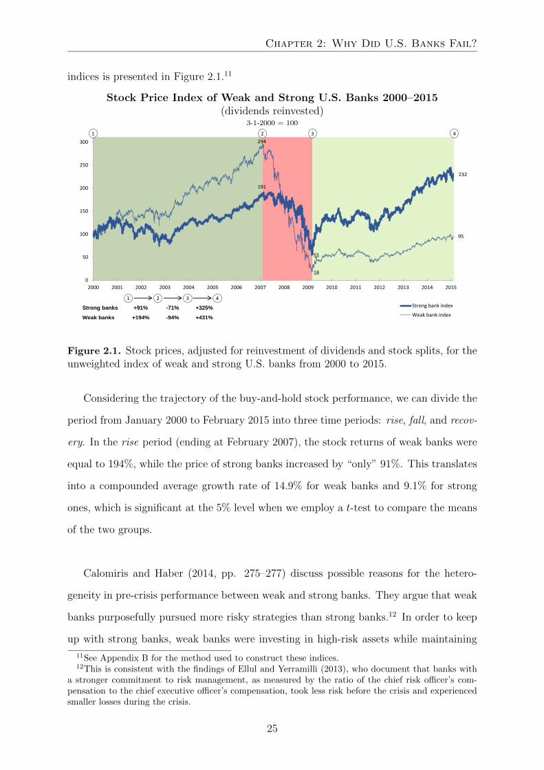
indices is presented in Figure 2.1.11
Stock Price Index of Weak and Strong U.S. Banks 2000–2015(dividends reinvested)
3-1-2000 = 100
191
55
232
294
18
95
0
50
100
150
200
250
300
2000 2001 2002 2003 2004 2005 2006 2007 2008 2009 2010 2011 2012 2013 2014 2015
Strong bank index
Weak bank index
Strong banks +91% -71% +325%
Weak banks +194% -94% +431%
1 2 3 4
1 42 3
Figure 2.1. Stock prices, adjusted for reinvestment of dividends and stock splits, for theunweighted index of weak and strong U.S. banks from 2000 to 2015.
Considering the trajectory of the buy-and-hold stock performance, we can divide the
period from January 2000 to February 2015 into three time periods: rise, fall, and recov-
ery. In the rise period (ending at February 2007), the stock returns of weak banks were
equal to 194%, while the price of strong banks increased by “only” 91%. This translates
into a compounded average growth rate of 14.9% for weak banks and 9.1% for strong
ones, which is significant at the 5% level when we employ a t-test to compare the means
of the two groups.
Calomiris and Haber (2014, pp. 275–277) discuss possible reasons for the hetero-
geneity in pre-crisis performance between weak and strong banks. They argue that weak
banks purposefully pursued more risky strategies than strong banks.12 In order to keep
up with strong banks, weak banks were investing in high-risk assets while maintaining
11See Appendix B for the method used to construct these indices.12This is consistent with the findings of Ellul and Yerramilli (2013), who document that banks with
a stronger commitment to risk management, as measured by the ratio of the chief risk officer’s com-pensation to the chief executive officer’s compensation, took less risk before the crisis and experiencedsmaller losses during the crisis.
25

Drivers of Bank Performance and The International Cost of Equity
only a thin layer of equity to cover for unexpected losses. Their strong counterparts,
on the other hand, were better positioned to invest in high-quality lower-risk projects
and maintained decent levels of equity. In addition to elevated levels of risk, weak banks
might have inflated their returns by increasing the size of government subsidies, such
as the explicit deposit insurance and the implicit too-big-to-fail guarantee (Calomiris &
Haber, 2014, p. 258). The largest banks with the lowest levels of equity, that is, the
ones with the largest government subsidies, experienced less scrutiny from depositors
and other creditors, which led to low borrowing costs and even lower levels of equity.
Considering that, in the run-up to the crisis, our median weak bank was two times larger
and held less equity than the median strong bank, this might also have been a contribut-
ing factor to the pre-crisis outperformance of weak banks.
In the next two years, 94% of the weak banks’ market value evaporates, whereas the
strong banks lose 71%. Hence, the loss in market value is in line with our classification
of weak versus strong banks. In the recovery period, it turns out that strong banks were
able to recover this loss in market value, to the extent that their stock prices in February
2015 were higher than before the start of the crisis. The weak banks recovered, as well,
but never come close to pre-crisis levels. In sum, weak banks significantly outperformed
strong banks in the years before the crisis. This reversed during the crisis when weak
banks lost almost all their market value. Furthermore, they were unable to recover to
pre-crisis levels in the six years after the crisis, whereas strong banks did recover.
2.2.3 Determinants of Strong Versus Weak Banks
In Section 2.2.1, we categorized banks as being either weak or strong. In this section, we
will focus on the underlying dynamics propelling organizational outcomes, which in our
case define the strength of the banks in question. To identify these dynamics, we use
a definition of institutions from the sociology literature: “Institutions are comprised of
regulative, normative and cultural-cognitive elements that, together with associated ac-
tivities and resources, provide stability and meaning to social life” (Scott, 2008, p. 48).
26

Chapter 2: Why Did U.S. Banks Fail?
This definition applies to institutions in general, ranging from divisions within a cor-
poration to non-governmental organizations and even supranational organizations. We
employ it in the context of a corporate organization – more specifically, a bank. The first
part of the definition focuses on the structure of organizations. This structure comprises
“legal, moral and cultural boundaries” (Scott, 2008, p. 50) that are meant to guide the
activities of the actors operating in an institution. Conversely, an organization might not
only limit actors, but also provide support with its resources. Furthermore, in addition
to restrictions and support, the actors’ own volition has an impact on organizational
outcomes. This contrast between agents, on the one hand, and structure, on the other,
has been a central debate in sociology for over a century and has more recently also found
its way to economics (e.g., Lawson, 1994) and management (e.g., Reed, 2005). Giddens
(1979) combines these opposing forces in his theory of structuration, in which structure
is interpreted as coagulated activities. However, although structure constrains the lat-
itude of actors, they are still able to influence organizational outcomes by determining
whether and how they will obey the rules. Conversely, their actions can ultimately lead
to adjustments in the rules, mores, and culture.
We will now transpose this view of an organization to the bank setting in order to
identify the underlying forces that might have caused these banks to perform strongly
or poorly during the crisis. Applying the structure and agency framework, we attempt
to measure structure according to the formal governance of the banks. While we are
aware that this measure of structure largely ignores moral and cultural components, un-
fortunately, these are much more challenging to measure and we must therefore discard
them.13 We operationalize the agency dimension as the behavior of employees.14 This
measuring of activities by employees in the multitude of instances in which they engage
is a formidable task, so we need to narrow it down. First, we restrict our attention to
13See, e.g., Zingales (2015a) in the introductory paper of the special issue of the Journal of FinancialEconomics dedicated to the NBER Conference on the Causes and Consequences of Corporate Culture.Here, corporate culture is not measured separately but is the aggregation of the personal beliefs andvalues of employees. In our view, such personal belief systems solely influence employee behavior and,consequently, do not pertain to the culture of a firm.
14A broader definition of actors would also, for instance, include customers, suppliers, and competitors.
27

Drivers of Bank Performance and The International Cost of Equity
CEOs, since they are the most important actors in an organization (Hambrick & Mason,
1984) and materially influence corporate outcomes (e.g., Bertrand & Schoar, 2003; Gra-
ham et al., 2013). Second, we focus on particular dimensions that drive the behavior of
CEOs.
The above discussion is graphically summarized in Figure 2.2. Arrow (1) shows the
impact of structure and agency on a bank’s strength. In addition to the structure and
agency factors, there are also external factors that influence that strength, such as the
economic growth in the area that a bank operates in.
Structure
Agency
Strength
External Factors
(1)
Figure 2.2. Theoretical framework of the firm, I. The strength of a bank is – ultimately– determined by its structure and agency, which is indicated by Arrow (1). Factorsthat influence a bank’s strength, but are not controlled by that bank, are designated asexternal factors.
In addition to this set-up, we follow the extant banking literature that relates a bank’s
financial characteristics to performance and survival (e.g., Beltratti & Stulz, 2012; Berger
& Bouwman, 2013; Fahlenbrach et al., 2012). This relation is depicted by Arrow (2) in
Figure 2.3.
28

Chapter 2: Why Did U.S. Banks Fail?
Structure
Agency
Strength
External Factors
(2)Financial Characteristics
Figure 2.3. Theoretical framework of the firm, II. We relate the strength of banksto their financial characteristics as depicted by Arrow (2). These characteristics areagain determined by structure and agency, as shown by the dashed arrow. Factorsthat influence a bank’s strength, but are not controlled by that bank, are designated asexternal factors.
Since we have argued that structure and agency determine organizational outcomes,
they also determine the financial characteristics of banks. As an example, consider the
finding of Berger and Bouwman (2013), who have shown a positive relationship between
the fraction of the balance sheet funded with equity and the probability of survival
during crisis times (Arrow [2]). Banks characterized by a cautious culture and/or a
more prudent CEO are likely to be more reluctant to choose high-leverage (dashed line),
which increases their odds of survival.
Structure
We use proxies to measure the formal governance of a bank’s structure. We were forced
by the availability of data to focus solely on these rule-based boundaries of firms and
ignore the moral and cultural restrictions. Good corporate governance practice implies
that power is not solely concentrated in the company’s management, but also shared with
shareholders. The rights of shareholders should be balanced with the decision rights of
management, and a good system of corporate governance should prevent “managerial
capitalism,” given that management has certain fiduciary duties towards its shareholders
as residual claimants of the firm (Shleifer & Vishny, 1997).
Weak banks were unable to withstand the financial crisis on their own, which was,
29

Drivers of Bank Performance and The International Cost of Equity
moreover, accompanied by a decline in stock prices of 94% (see Figure 2.1). Therefore, ex
post, their shareholders must have been unhappy with outcomes, which could have been
attributed to inadequate formal governance at these banks. However, this is not in line
with Beltratti and Stulz (2012), Erkens et al. (2012), and Fahlenbrach and Stulz (2011),
who found a negative relationship between quality of governance (shareholder-friendliness
of boards, alignment of CEO and shareholders, level of institutional ownership) and per-
formance during the crisis. The negative relationship between quality of governance and
performance during the crisis does not extend to the risk governance of banks. Ellul
and Yerramilli (2013) documented a positive relationship between the strength and in-
dependence of the risk management function within a bank, on the one hand, and stock
returns and operating performance during the crisis, on the other. In sum, although
some facets of corporate governance seem not to have been in the long-term interests
of shareholders, centrality of risk management was key to the crisis performance of banks.
To assess the impact of governance on bank strength, we focus on two dimensions:
shareholder rights vis-a-vis management power and CEO duality. We employ the Gov-
ernance Index of Gompers, Ishii, and Metrick (2003) to measure shareholder rights. The
index consists of 24 corporate governance provisions related to shareholder rights, with
each restriction regarding these rights associated with an increase of one index point.
Hence, a high score reflects limited rights for shareholders and, thus, extensive rights
for management. We compare the Governance Index of weak and strong banks. Since
Beltratti and Stulz (2012) and Erkens et al. (2012) found a negative relationship between
board independence and stock performance during the crisis, we likewise expect to find
that according to our measure, weak banks, with their strongly underperforming stock
returns during the crisis (see Section 2.2.2), were better governed than strong banks.
In addition, we consider the impact of differences in CEO Duality on a bank’s
strength. The argument against a combined role for CEO and chairman is motivated by
agency theory, since it concentrates executive and non-executive power in a single person
30

Chapter 2: Why Did U.S. Banks Fail?
and implies less internal monitoring of the CEO. Consequently, the trend in the U.S. is
a decrease in the practice of combining these roles: from more than 80% in the early
1990s to just over 50% in 2010 (Yang & Zhao, 2014). Despite this trend and the theoret-
ical arguments for separating these two roles, a meta-analysis of 48 studies by Krause,
Semadeni, and Cannella (2014) documents no positive relationship between separating
these roles and firm performance. Hence, a priori, we do not expect a clear difference
between weak and strong banks in this dimension.
Agency
The second driver of organizational outcomes is the agency of employees. Although it
would have been highly informative to have gained insight into the behavior of all of
the banks’ executives (and even better all employees), we focus here on the behavioral
drivers of the CEOs, since they hold the most powerful position within an organiza-
tion (Hambrick & Mason, 1984) and strongly influence corporate outcomes (Bertrand
& Schoar, 2003; Graham et al., 2013). Furthermore, the availability of data impedes a
broader scope. Since the drivers of CEO behavior are myriad, we chose to focus our
analysis on the following two: executive remuneration and socioeconomic background.
We selected remuneration because it is perceived to have been an important cause of the
financial crisis (Diamond & Rajan, 2009), and we want to establish whether our results
are in line with earlier findings relating remuneration practices to the crisis. While the
topic of remuneration may have already been well researched, we are, to the best of our
knowledge, the first to research the impact of a CEO’s socioeconomic background on
bank performance during the financial crisis. The recent interest in the management
literature regarding the explanatory power of this variable for firm-level outcomes (Kish-
Gephart & Campbell, 2015) motivates us to investigate its relevance in explaining bank
strength.
Remuneration. Remuneration packages for CEOs are meant to financially and strate-
gically align CEOs with the firm’s shareholders and thereby solve the underlying principal-
31

Drivers of Bank Performance and The International Cost of Equity
agent problem.15 In contrast to this theoretical motivation, Bebchuk and Fried (2004)
argue that the maximum level of compensation is only constrained by public outrage:
that is, bonuses are of no use in motivating CEOs but are instead used to extract rents,
which ultimately harms the long-term interests of a firm and its shareholders.
Compensation has also often been raised as one of the main causes of the financial
crisis. For instance, Kirkpatrick states that the remuneration before and during the fi-
nancial crisis was in some cases not in line with “the strategy and risk appetite of the
company and its longer term interests” (2009, p. 1). Furthermore, Diamond and Ra-
jan (2009) indicate that remuneration tended to be based on short-term risk-adjusted
performance, which stimulated bank employees to search for excessive returns that were
not recognized by the financial system as being risky. In hindsight, the high returns
should have been interpreted as the compensation for the default risk of the underlying
mortgage contracts. Despite these conjectures, Fahlenbrach and Stulz (2011) show that
banks with more option compensation or a larger fraction of cash bonus relative to a
guaranteed salary did not perform worse during the crisis. This poses a challenge to the
notion of executive compensation being a major cause of the crisis.
An alternative explanation of compensation not being positively related to crisis per-
formance is the CEOs’ large cashing-out from 2000 to 2008, which diminished the effec-
tiveness of incentive-based compensation. This practice was significantly more prevalent
at the fourteen largest U.S. financial institutions receiving government aid than at the
banks that survived the crisis independently (Bhagat & Bolton, 2014). Insofar as the
high cashing-out was preceded by large remuneration and banks receiving government
support performed poorly during the crisis, the performance during the crisis is likely
to have been negatively related to pre-crisis remuneration. This relationship is possibly
mediated by the higher pre-crisis riskiness of weak crisis performers (Fahlenbrach et al.,
2012). Alternatively, a non-causal explanation for the association between compensa-
15See Murphy (1999) for a review of the literature that considers executive compensation to be thesolution to the principal-agent problem of shareholders vis-a-vis CEOs.
32

Chapter 2: Why Did U.S. Banks Fail?
tion and riskiness is formulated by Cheng, Hong, and Scheinkman (2015), who provide
evidence that riskier firms need to convince risk-averse CEOs to supply their labor to
compensate for the additional riskiness. Overall, the evidence suggests a negative rela-
tionship between compensation and crisis performance.
Remuneration of CEOs comprises three main categories: Fixed Salary, Cash Bonus,
and Delayed Bonus.16 Based on the evidence presented above, we expect a higher Cash
Bonus (typically associated with short-term incentives) and Delayed Bonus for weak
banks than for strong banks. Moreover, given that Fixed Salary only comprises a small
fraction of total compensation, we do not expect a difference between weak and strong
banks. Furthermore, similar to Fahlenbrach and Stulz (2011), we compare the Cash
Bonus to Fixed Salary for weak and strong banks to measure the relative importance of
short-term incentives. An alternative way to measure this relative importance is given
by the proportion of Cash Bonus to Delayed Bonus. Moreover, the use of these ratios
alleviates the concern that differences in the magnitude of remuneration packages are
driven by size differences among the banks.17 Since we expect both a higher Cash Bonus
and Delayed Bonus at weak banks, the former ratio is expected to be higher for weak
banks, while this is unclear for the latter ratio.
CEO’s Socioeconomic Background. There is a diverse and growing literature that
deals with the impact of family background on career success, personal characteristics,
and firm-level outcomes. When studying intergenerational mobility, an individual’s class
of origin (i.e., family background), as measured in economics by paternal or household
income (Solon, 2002) and in sociology by the father’s type of employment (Erikson &
Goldthorpe, 2002), is related to his/her class of destination. Although there are cross-
country differences (Solon, 2002), the general conclusion is that there is a significant
positive correlation between the class of origin and class of destination. In the finance lit-
erature, Mullins and Schoar (2016) investigated the family backgrounds of different types
16This category comprises restricted stock, stock options, and pension income.17Gabaix and Landier (2008) document a positive relationship between company size and the magni-
tude of the remuneration package.
33

Drivers of Bank Performance and The International Cost of Equity
of CEOs in 22 emerging markets. They found that founder CEOs of family firms and
professional18 CEOs of non-family firms are more likely to be from lower socioeconomic
classes than CEOs related to the founder or current shareholders and professional CEOs
of family firms. Therefore, they suggest that, in emerging economies, founder CEOs
of family firms and professional CEOs of non-family firms provide a means of upward
mobility in the social hierarchy.
In the above studies, social class features both as a dependent and independent vari-
able. However, class of origin has also been used as an independent variable to explain
personal characteristics. For example, individuals from a higher class are associated
with better health (Duncan, Ziol-Guest, & Kalil, 2010) and are more ambitious (Bow-
den & Doughney, 2010) than individuals from a lower-class. However, Martin, Cote,
and Woodruff (2016) demonstrate that social class is negatively related to leadership
effectiveness. This relationship is mediated by the higher levels of narcissism observed
in individuals raised in an upper-class environment.
The final category of research we consider is the literature focusing on the impact of
family background on firm-level outcomes. This literature fills a gap identified by Ham-
brick and Mason: “There has been almost no attempt in the organizational literature
to relate socioeconomic background to organizational strategy or performance” (1984,
p. 201). To the best of our knowledge, the Kish-Gephart and Campbell (2015) study
is the only one in this area. In it, the authors hypothesize that people from the lower-
and upper-classes are more risk-seeking, which subsequently translates into higher risk-
taking at the firm level. They argue that the early-life experience of having “nothing to
lose” (lower-class) or having a safety net (upper-class) determines prospective attitudes
towards risk. This contrasts with people raised in the middle-class, in an environment
where parents were concerned with the avoidance of risk in order to keep their job.
Their empirical analysis convincingly shows that CEOs from the upper-class engage in
18“Professional” meaning an outside manager who is neither the founder nor related to the founder’sor shareholders’ family/families.
34

Chapter 2: Why Did U.S. Banks Fail?
the most risk-taking compared to CEOs from the lower- and middle-classes.
Therefore, combining the results of a negative relationship between pre-crisis bank
risk and crisis performance (Fahlenbrach et al., 2012) with the poor stock returns of
our weak banks during the crisis (see Section 2.2.2), we expect more upper-class CEOs
– associated with higher risk-taking according to Kish-Gephart and Campbell (2015) –
at weak banks than at strong banks. The opposite reasoning applies to middle-class
CEOs. Finally, since the relationship between risk-taking and lower-class background is
weaker in Kish-Gephart and Campbell (2015), we have no a priori expectations on the
distribution of lower-class CEOs among weak and strong banks.
Following Mullins and Schoar (2016) and Kish-Gephart and Campbell (2015), we
categorize our CEOs into lower-, middle-, and upper-class categories according to a
simplified version of the classification system using paternal professions (see Erikson &
Goldthorpe, 2002).
Financial Characteristics
In this section, we introduce the financial characteristics we chose for comparing weak
and strong banks. We also predict their expected impact on bank strength (see Figure
2.3). In Section 2.2.1, we argued that weak banks would not have survived the crisis
without state support. We therefore regard them as failing banks, in contrast to the
strong banks that would have survived the crisis independently. Although our sample
size is much smaller, our setup is closely related to that of Cole and White (2012),
who compared failing banks to surviving ones in the U.S. after the financial crisis. In
selecting our variables, therefore, we largely followed their approach and focused on
capital adequacy, assets quality, earnings, liquidity, growth, and size.19
19This selection covers four of the six constituents of the CAMELS rating. That rating is used by U.S.regulators to determine the viability of banks and is composed of: Capital Adequacy, Asset Quality,Management, Earnings, Liquidity, and Sensitivity to the Market.
35

Drivers of Bank Performance and The International Cost of Equity
Capital Adequacy. We measured capital adequacy by Equity to Assets and the Tier
1 Ratio20 – Tier 1 capital to risk-weighted assets. The higher these ratios, the larger the
bank’s cushion to cover unexpected losses and the more likely it is to survive. Berger and
Bouwman (2013) have shown that for large banks, this applies mainly during periods of
banking crisis. Therefore, we expect higher ratios at strong banks than at weak banks
before the crisis. Moreover, in the multivariate analysis, we expect a positive relationship
between capital adequacy and the probability of strength for banks.
Additionally, we consider Debt to Assets, which together with deposits and equity,
covers the liability side of the balance sheet. Hence, the larger the fraction of the balance
sheet funded with debt, the smaller the deposit base. Since deposits are a stable and
cheap form of funding, and the fraction of deposits is inversely related to the fraction of
debt, we expect a larger fraction of debt to assets at weak banks.
Asset Quality. The assets of banks mainly comprise loans and securities. Although
mortgage backed securities (MBS) were the direct cause of the financial crisis, several
studies have shown a negative relationship between Loans to Assets (or positive one
for Securities to Assets) and bank performance during the crisis (Beltratti & Stulz,
2012; Cole & White, 2012; Fahlenbrach et al., 2012). This is likely because MBS only
constituted a small portion of the total securities on the balance sheet, while other
securities such as bonds are generally regarded as safe assets (Cole & White, 2012).
Therefore, we predict a higher fraction of Loans to Assets at weak banks.
Earnings. The profitability of a bank is positively related to its chance of survival,
since that is what allows the bank to invest in order to remain competitive or add equity
to strengthen its balance sheet. Therefore, in line with results from Berger and Bouwman
(2013) and Cole and White (2012), we expect higher profitability for strong than for weak
20The Tier 1 capital ratio is the ratio regulators primarily focus on in assessing a bank’s capitaladequacy.
36

Chapter 2: Why Did U.S. Banks Fail?
banks, as measured by Return on Assets or Return on Equity.
Liquidity. During the financial crisis, liquidity was a major problem for banks (Bel-
tratti & Stulz, 2012; Brunnermeier, 2009; Diamond & Rajan, 2009) and the mechanism
through which distress spread throughout the system (Brunnermeier, 2009). This was
primarily caused by the banks’ dependency on short-term (ST) debt. The need to rollover
this debt in the short term makes a bank vulnerable to liquidity shortages, which could
ultimately lead to default. In order to quantify this dependency, we use ST Debt to
Assets, and we expect larger values for weak banks than for strong banks.
Growth. Fahlenbrach et al. (2012) showed that bottom performers during the crisis
grew significantly faster before the crisis than top performers. They argue that this
Asset Growth most likely occurred in risky assets. Kedia and Philippon (2009) provide
another interpretation for their finding, which is that weak banks were willing to keep
up with the growth of strong banks even though they did not have the same positive
NPV projects as strong banks. Hence, we expect that weak banks grew faster before the
crisis than strong banks.
Size. The final financial characteristic we consider is the Assets size of the bank. Larger
firms are – on average – organizationally more complex, bureaucratic, and susceptible
to internal agency conflicts, which makes them harder to lead. On the other hand, they
might also benefit from economies of scale. Therefore, a priori, we do not expect size
differences between weak and strong banks.
2.3 Data
In this section, we present our data. Table 2.2 provides an overview of the data sources
and years covered per variable.
37

Drivers of Bank Performance and The International Cost of Equity
Table 2.2. Variables, data sources, and years covered.
Variable Source Years
StructureGovernance Index IRRC 2002, 2004, 2006CEO Duality ExecuComp 2002–2006
AgencyRemuneration ExecuComp 2002–2006Socioeconomic Background Internet search 2002–2006
Financial Characteristics Bloomberg 2002–2006
Market PerspectiveStock Prices Bloomberg 2000–2015
The first column of Table 2.2 corresponds to the categorizations presented in Section
2.2.3. The data cover the 2002–2006 period for all variables, except for the stock prices,
which cover the period from January 2000 to February 2015.
The Governance Index was constructed using data from the Investor Responsibility
Research Center (Gompers et al., 2003), which are made available on Andrew Metrick’s
website (see http://faculty.som.yale.edu/andrewmetrick/data.html). These data
were not updated annually, only at seven points between 1990 and 2006. In this chapter,
we use the data for the years 2002, 2004, and 2006.
The CEO Duality data were collected from ExecuComp. A score of 1 indicates that
the CEO is also the Chairman of the Board, otherwise the score is 0. If a succession
occurred during the period under consideration (2000–2006), the CEO Duality “score”
given was that of the CEO in charge for the longest portion of the year. We thus assume
that the CEO in charge for the greater part of the year influences firm performance the
most. If the succession took place on June 30 or July 1 – that is, exactly in the middle
of the year – the observation was excluded.
Remuneration data were also collected from ExecuComp. Fixed Salary and Cash
38

Chapter 2: Why Did U.S. Banks Fail?
Bonus are individually specified in the database.21 To compute the Delayed Bonus, we
deducted the Fixed Salary and Cash Bonus from Total Compensation, for which we
used the ExecuComp variable Total Compensation (Salary + Bonus + Other Annual
+ Restricted Stock Grants + LTIP Payouts + All Other + Value of Option Grants).
If a succession occurred during the year under study, the compensation of the CEO in
charge for the longest portion of the year was used. If the succession took place exactly
in the middle of the year, the compensation amounts for the predecessor and successor
were averaged.
In order to identify the CEOs’ fathers’ professions and determine their Socioeconomic
Background, we conducted an internet search. We also approached organizations that
these former CEOs currently work for to obtain additional information. In cases where a
succession occurred in the period from 2002 to 2006, we took the professions of the fathers
of both CEOs into consideration in our analysis. Finally, Financial Characteristics and
Stock Prices were obtained from Bloomberg.
2.4 Methodology
We analyzed differences between weak and strong banks using both univariate and mul-
tivariate analysis.
2.4.1 Univariate Analysis
We compared the averages for weak and strong banks per variable and per year. For
instance, the average of the Governance Index of weak banks in 2002 is compared to
the average of strong banks in 2002. The variables we considered were categorized into
21An adjustment was made to the Cash Bonus category in 2006. Starting that year, a new variable,Non-Equity Incentive Plan Compensation, was reported in the ExecuComp database, which was alsopart of the Cash Bonus. This is confirmed by the summary compensation table of Citigroup’s DEF14ASEC filings for 2006, in which the Cash Bonus entry has been replaced by this new variable. However,since the Cash Bonus variable in ExecuComp is not equal to 0 for all banks in 2006, we added togetherthe Cash Bonus and Non-Equity Incentive Plan Compensation variables from ExecuComp to form ourCash Bonus variable for 2006.
39

Drivers of Bank Performance and The International Cost of Equity
continuous, unordered discrete, and ordered discrete variables, and we applied a specific
univariate method for each category.
For the continuous variables, the averages were compared using the student t-test
developed by Welch (1947). That test allows sample sizes and variances of the weak and
strong banks to be unequal. To compare the unordered discrete variables (e.g., CEO
Duality) for weak and strong banks, we employed Fisher’s exact test (R. A. Fisher, 1935).
The test is exact in the sense that the p-value does not rely on the sampling distribution
of the test statistic becoming equal to the limiting distribution as the sample size goes to
infinity. This is especially relevant considering our small sample size. Finally, we applied
the Wilcoxon-Mann-Whitney test (Mann & Whitney, 1947; Wilcoxon, 1945) to compare
the ordered discrete variables between weak and strong banks. This nonparametric test
assesses whether two samples are drawn from the same or different populations. With
regard to a CEO’s Socioeconomic Background, the test compares whether the weak
bank’s sample is from the same population as the strong bank’s sample, for example.
2.4.2 Multivariate Analysis
In addition to the univariate analysis, we conducted a multivariate analysis to identify
differences between weak and strong banks. To do so, we employed a logit model where
weak banks are designated as 0 and strong banks as 1. To account for any correlation
between observations of the same bank in consecutive years (2002–2006), the error terms
were clustered at the bank level (Petersen, 2009).
2.5 Results
The structure of the results section is similar to Section 2.2.3, in that we start with the
discussion of the structure and agency variables and their impact on bank strength (see
Arrow [1] in Figure 2.2) and then shift our attention to the financial characteristics (see
Arrow [2] in Figure 2.3).
40

Chapter 2: Why Did U.S. Banks Fail?
2.5.1 Structure
We start by comparing weak and strong banks on the quality of the formal governance
as measured by the Governance Index from Gompers et al. (2003) and CEO Duality.
Table 2.3 presents the average Governance Index for the weak and strong banks per
year (left-hand columns) and the number of weak and strong banks where the roles of
CEO and chairman were combined (right-hand columns), with the total number of banks
under consideration in that category shown in parentheses.
Table 2.3. Quality of formal governance of weak and strong banks. In the left-handsection of the table, the weak and strong columns contain the Governance Index averagesfor the weak and strong banks per year. The bottom line is the average over the years.In the right-hand section of the table, the # weak and # strong columns contain thenumber of banks where the roles of CEO and chairman were combined, with the totalnumber of observations in parentheses. The p-values in the left-hand section correspondto the Welch t-test and in the right-hand section to Fisher’s exact test (see Section 2.4.1.)
Governance Index weak strong p-value2002 9.6 9.8 0.880
2004 9.5 9.9 0.730
2006 9.4 9.1 0.772
average 9.5 9.6 0.939∗ p < 0.10, ∗∗ p < 0.05
CEO Duality # weak # strong p-value2002 13 (15) 8 (8) 0.5262003 14 (15) 8 (8) 1.0002004 13 (15) 8 (8) 0.5262005 12 (14)22 8 (8) 0.5152006 13 (15) 8 (8) 0.526
The division of power between shareholders and management was measured using
the Governance Index of Gompers et al. (2003), where a higher score corresponds to
more limitations on the rights of shareholders and thus more power for management. In
the spirit of Shleifer and Vishny (1997), who state that it is the role of governance to
assure a return on investment for shareholders, fewer rights for that group is regarded
as constituting poor governance. There is no significant difference between strong and
weak banks in any of the years. Moreover, in two of the three years, the shareholders
of weak banks had even more rights than the shareholders of strong banks. Hence, our
results are in line with the earlier findings of Beltratti and Stulz (2012) and Erkens et
22Keycorp was excluded from the sample in 2005 because the CEO stepped down in the middle ofthe year.
41

Drivers of Bank Performance and The International Cost of Equity
al. (2012), who found a negative relationship between performance during the crisis and
the shareholder-friendliness of a board.23
The combination of the roles of CEO and chairman is, from a governance perspective,
unfavorable, since the CEOs must then supervise themselves in their role of chairman.
This concentration of power can hamper effective supervision. Our results suggest that
CEO Duality is not a differentiating characteristic between weak and strong banks. At
strong banks, the roles were combined in all of the years, while they were separated at
only two weak banks in all of the years, except for 2003, when only one CEO was not
also the chairman. However, none of the differences are statistically significant at the
conventional levels. Therefore, consistent with the conclusion of Krause et al. (2014), we
found no significant relationship between CEO Duality and performance. In sum, with
regard to the structural dimension, weak and strong banks did not differ substantially
in the years leading up to the financial crisis. In the next section, we turn our attention
to the agency dimension.
2.5.2 Agency
We focused on the remuneration and socioeconomic background of CEOs as a proxy for
agency.
Remuneration
Table 2.4 contains the average yearly Fixed Salary, Cash Bonus, Delayed Bonus, and
Total Remuneration for CEOs at the banks studied. Furthermore, in the bottom sections
of the table, we document the ratios of Cash Bonus to Fixed Salary and Cash Bonus to
Delayed Bonus.
23The negative relationship between the quality of formal corporate governance and crisis performancethat we and previous studies (e.g. Beltratti & Stulz, 2012; Erkens et al., 2012) have documented, mightsuffer from an endogeneity issue. If, in the run-up to the crisis, weak banks’ shareholders did not confidein their management they might have demanded and received more shareholder rights to be better ableto control management. Strong banks with their superior strategy might have been able to convince theirshareholders without the need to grant additional shareholder rights. This is an alternative, non-causalinterpretation of the negative relationship between governance quality and crisis performance.
42
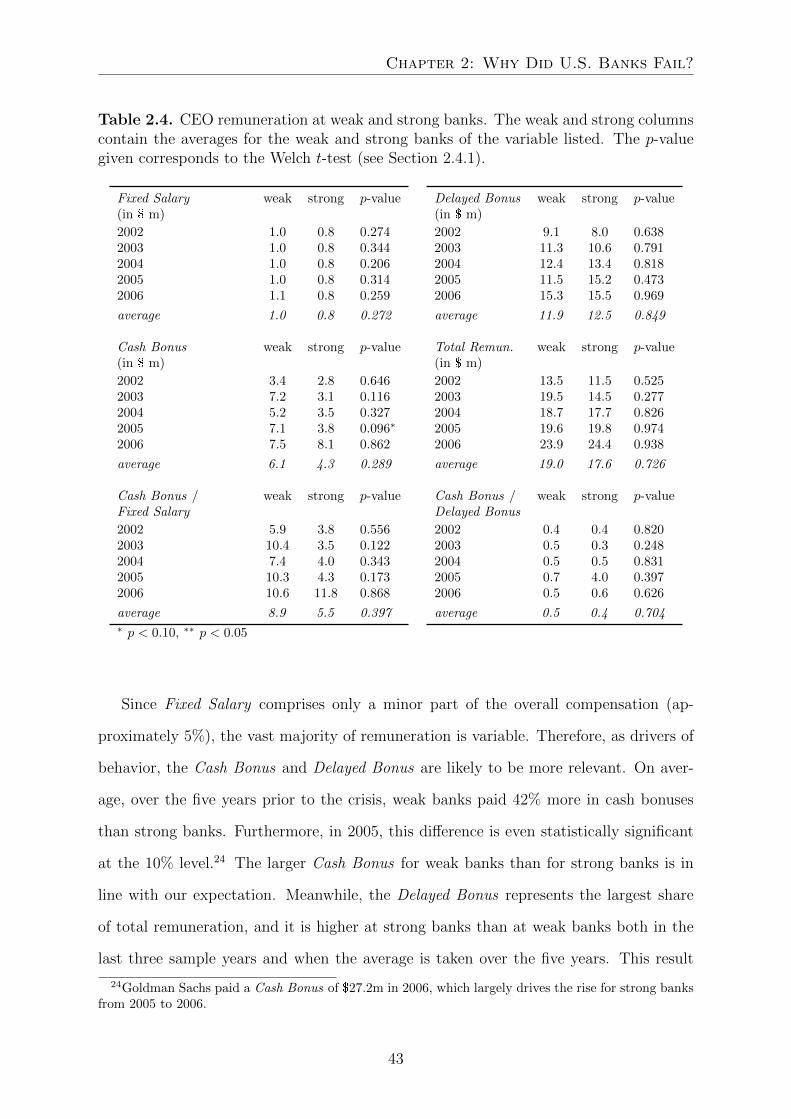
Chapter 2: Why Did U.S. Banks Fail?
Table 2.4. CEO remuneration at weak and strong banks. The weak and strong columnscontain the averages for the weak and strong banks of the variable listed. The p-valuegiven corresponds to the Welch t-test (see Section 2.4.1).
Fixed Salary weak strong p-value(in $ m)
2002 1.0 0.8 0.2742003 1.0 0.8 0.3442004 1.0 0.8 0.2062005 1.0 0.8 0.3142006 1.1 0.8 0.259
average 1.0 0.8 0.272
Cash Bonus weak strong p-value(in $ m)
2002 3.4 2.8 0.6462003 7.2 3.1 0.1162004 5.2 3.5 0.3272005 7.1 3.8 0.096∗
2006 7.5 8.1 0.862
average 6.1 4.3 0.289
Cash Bonus / weak strong p-valueFixed Salary
2002 5.9 3.8 0.5562003 10.4 3.5 0.1222004 7.4 4.0 0.3432005 10.3 4.3 0.1732006 10.6 11.8 0.868
average 8.9 5.5 0.397∗ p < 0.10, ∗∗ p < 0.05
Delayed Bonus weak strong p-value(in $ m)
2002 9.1 8.0 0.6382003 11.3 10.6 0.7912004 12.4 13.4 0.8182005 11.5 15.2 0.4732006 15.3 15.5 0.969
average 11.9 12.5 0.849
Total Remun. weak strong p-value(in $ m)
2002 13.5 11.5 0.5252003 19.5 14.5 0.2772004 18.7 17.7 0.8262005 19.6 19.8 0.9742006 23.9 24.4 0.938
average 19.0 17.6 0.726
Cash Bonus / weak strong p-valueDelayed Bonus
2002 0.4 0.4 0.8202003 0.5 0.3 0.2482004 0.5 0.5 0.8312005 0.7 4.0 0.3972006 0.5 0.6 0.626
average 0.5 0.4 0.704
Since Fixed Salary comprises only a minor part of the overall compensation (ap-
proximately 5%), the vast majority of remuneration is variable. Therefore, as drivers of
behavior, the Cash Bonus and Delayed Bonus are likely to be more relevant. On aver-
age, over the five years prior to the crisis, weak banks paid 42% more in cash bonuses
than strong banks. Furthermore, in 2005, this difference is even statistically significant
at the 10% level.24 The larger Cash Bonus for weak banks than for strong banks is in
line with our expectation. Meanwhile, the Delayed Bonus represents the largest share
of total remuneration, and it is higher at strong banks than at weak banks both in the
last three sample years and when the average is taken over the five years. This result
24Goldman Sachs paid a Cash Bonus of $27.2m in 2006, which largely drives the rise for strong banksfrom 2005 to 2006.
43

Drivers of Bank Performance and The International Cost of Equity
is different from our expectation and indicates that remuneration at strong banks was
more geared towards the long term than it was at weak banks.
In the lowest two sections of the table, we compare the ratios of Cash Bonus to Fixed
Salary and Cash Bonus to Delayed Bonus. This presents two advantages over the com-
parison of the absolute numbers. First, the use of ratios alleviates the concern that the
differences in the sizes of the remuneration packages were caused by differences in the
sizes of the banks.25 Second, it provides a way of measuring the short-term incentives
(Cash Bonus) relative to unconditional remuneration (Fixed Salary) and long-term in-
centives (Delayed Bonus). The Cash Bonus to Fixed Salary variable averaged over five
years is more than 60% higher at weak banks than at strong banks.26 This difference is
largely driven by two outliers, Bear Stearns and Merrill Lynch, where the Cash Bonus
was 58 times and 16 times larger, respectively, than the Fixed Salary. Although the dif-
ference is less pronounced, the ratio of Cash Bonus to Delayed Bonus is approximately
12% larger at weak banks than at strong banks.27
Weak banks paid higher Cash Bonuses than strong banks, both in absolute and
relative terms. Moreover, strong banks granted more bonuses geared towards the long
term. Therefore, relative to the CEOs of strong banks, the CEOs of weak banks were
more incentivized to focus on short-term gains, rather than on the long-term well-being
of the bank.28
25The median weak bank is almost 2.5 times larger than the median strong bank (see Table 2.1).26We excluded the CEO of Capital One (strong bank) in this analysis because the Fixed Salary and
Cash Bonus are both equal to 0 in all the years.27The high value for strong banks in 2005 is driven by The Bank of New York Mellon, with a ratio of
Cash Bonus to Delayed Bonus of 30. This is not reflected in the average over the five years, because incomputing it, we first averaged over the years and then over the banks.
28The difference in riskiness between weak and strong banks might also account for the differences inremuneration. Imagine the situation where a risk-averse CEO has to choose between leading a strongor a weak bank. When the CEO is aware of the weak bank’s higher riskiness, the risk-averse CEO isonly willing to work for this bank, and forgoing the possibility to work for the less risky strong bank, ifhe is financially compensated for this additional risk. This would be an alternative explanation for thehigher Cash Bonus at weak banks. Moreover, the lower Delayed Bonus at weak banks is consistent withthis explanation. For weak banks, the Delayed Bonus is a relatively costly way to compensate theirrisk-averse CEOs, since they substantially discount the future cash flows stemming from the DelayedBonus to incorporate the banks’ higher riskiness. Therefore weak banks prefer to compensate theirCEOs in cash.
44

Chapter 2: Why Did U.S. Banks Fail?
CEO’s Socioeconomic Background
In this section, we shift our attention to the early stages of a CEO’s life. This analysis
contributes to the relatively novel literature that relates the socioeconomic background of
CEOs to their decisions at the company level (Kish-Gephart & Campbell, 2015). In our
approach, we measure a CEO’s class background according to the status of his father’s
profession, which we divide into lower-, middle-, and upper-classes by applying a simpli-
fied version of the categorization identified by Erikson and Goldthorpe (2002). Tables
2.5 and 2.6 list the CEOs, fathers’ professions, and classes of the paternal professions for
the weak and strong banks, respectively.
Table 2.5. The classification of the CEOs’ fathers’ professions – weak banks. Professionsof the fathers of the CEOs at weak banks in the 2002–2006 period and their correspondingclass: 0 = lower-class; 1 = middle-class; and 2 = upper-class.
Weak Banks CEO Father’s Profession Class
Citigroup Charles Prince III Plasterer 0
Sanford I. Weill Dress manufacturer 0
Bank of America Kenneth D. Lewis Lumberyard poultry plant, army 0
Merrill Lynch E. Stanley O’Neal Assembly line 0David H. Komansky Post office job 0
Wachovia G. Kennedy Thompson Manager at textile mill 1
Lehman Brothers Richard S. Fuld Jr. Army officer 1
Wells Fargo Richard M. Kovacevich Sawmill worker 0
Bear Stearns James E. Cayne Patent attorney 2
Washington Mutual Kerry K. Killinger Musician and musical teacher 0
Countrywide Angelo R. Mozilo Butcher 0
Suntrust L. Phillip Humann Job at oil-and-gas shipper 029
National City David A. Daberko
Regions Financial C. Dowd RitterJackson W. Moore Medical doctor 2Carl E. Jones, Jr.
PNC Financial James E. Rohr Small restaurant owner 030
Fifth Third Bancorp George A. Schaefer, Jr.
Keycorp Henry L. Meyer, III
45

Drivers of Bank Performance and The International Cost of Equity
Table 2.6. The classification of the CEOs’ fathers’ professions – strong banks. Pro-fessions of the fathers of the CEOs at strong banks in the 2002–2006 period and theircorresponding class: 0 = lower-class; 1 = middle-class; and 2 = upper-class.
Strong Banks CEO Father’s Profession Class
JPMorgan Chase James Dimon Stockbroker, exec. vice pres. AmEx 2William B. Harrison Jr. Peoples Bank, real estate developm. 1
Goldman Sachs Lloyd C. Blankfein Bakery truck driver, clerk 0Henry M. Paulson Jr. Wholesale jeweler 1
U.S. Bancorp Richard K. DavisJerry A. Grundhofer Bartender 0
Capital One Financial Richard D. Fairbank Physics professor 2
American Express Kenneth I. Chenault Dentist 2
BB&T John A. Allison IV
State Street Ronald E. LogueDavid A. Spina
Bank of NY Mellon Thomas A. Renyi Medical doctor 2
These tables show that the CEOs of the weak banks more frequently came from the
lower-class than those of the strong banks: 10 of the 14 weak banks’ CEOs came from
a lower-class background compared to two of the eight CEOs of the strong banks. Con-
versely, half of the CEOs of the strong banks were from the upper-class compared to
only two at the weak banks. The remaining two CEOs in both groups were raised in a
middle-class environment.
To determine whether this difference in the CEOs’ socioeconomic background was
also statistically significant, we employed the Wilcoxon-Mann-Whitney test (see Section
2.4.1). This test determines the likelihood that the weak and strong banks’ samples were
drawn from the same population, assuming an equal probability of CEOs being raised
in one of the three classes. This test (with a p-value equal to 0.034) rejected the null hy-
29We have not been able to find more specific information regarding the nature of the job. It istherefore difficult to judge whether it was a higher or lower ranking job at the oil-and-gas company.Even if the class of the job were to be changed from 0 to 1, the class difference between the weak andstrong banks’ CEOs would remain significant, with a p-value of 0.054.
30The profession is classified as 0 because his father passed away when he was 10 and his motherwas not able to keep the restaurant. Under normal circumstances, a small restaurant owner would havebeen classified as 1.
46

Chapter 2: Why Did U.S. Banks Fail?
pothesis that the samples were drawn from the same population. We therefore conclude
that the CEOs of weak banks were raised in a lower-class environment significantly more
often than their counterparts at strong banks. This is not in line with our expectation,
since we expected to find more upper-class CEOs at the riskier weak banks, based on the
results of Kish-Gephart and Campbell (2015). One possible explanation for this could
be the difference in samples: Kish-Gephart and Campbell used S&P 1500 companies,
whereas we focused exclusively on the largest U.S. banks.
At this point we want to investigate the possibility that strong banks, with their
upper-class CEOs, were favored by regulators in the stress test discussed in Section 2.2,
which potentially distorts our classification of the banks. Before we discuss possible
ways in which this might have occurred, we assess the trustworthiness of the stress test.
According to Acharya, Pedersen, Philippon, and Richardson (2017) the stress test was
“generally considered to be a credible test” (p. 17), which is the first indication that
regulators were not favoring certain banks. However, other concerns remain. The stress
test assessed the capital adequacy of banks in an adverse economic scenario (see Section
2.2). Two critiques that have often been voiced regarding capital adequacy measures of
banks is the use of book values of equity instead of market values and risk weighted assets
instead of total assets (Acharya, Engle, & Pierret, 2014; Calomiris & Herring, 2013).
These critiques also pertain to the SCAP. Therefore, we resort to an alternative measure
of bank strength, called SRISK, which has been introduced by Brownlees and Engle
(2017) and Acharya, Engle, and Richardson (2012), to compute the expected equity
shortfall per bank when a systemic crisis hits. In Table 2.7 we present this shortfall
divided by total assets on December 31, 2008,31 which we obtain from the Volatility
Institute at the NYU Stern School of Business,32 for the banks in our sample that were
still active at that time. These shortfalls are computed when the market declines with
40% and the minimum required equity to assets ratio for banks equals 4%.
31This is the same date as the starting point used in the SCAP.32See http://vlab.stern.nyu.edu/welcome/risk/.
47

Drivers of Bank Performance and The International Cost of Equity
Table 2.7. The expected equity shortfall of weak and strong banks, using SRISK(Acharya et al., 2012; Brownlees & Engle, 2017), relative to their assets as of December31, 2008. The equity shortfall is computed assuming that the market declines with 40%and banks are required to have at least 4% of equity to assets. Banks are ordered withrespect to their relative expected equity shortfall.
Institution Weak / Strong Equity Shortfallto Assets
Citigroup Weak 3.22%Wachovia Weak 3.15%Merrill Lynch Weak 3.04%National City Weak 2.03%Goldman Sachs Strong 1.90%Bank of America Weak 1.86%KeyCorp Weak 1.65%JPMorgan Chase Strong 1.61%Regions Financial Weak 1.30%Fifth Third Bancorp Weak 1.08%SunTrust Banks Weak 0.38%PNC Financial Weak 0.08%Capital One Financial Strong 0.00%Wells Fargo Weak -0.94%State Street Strong -1.64%BB&T Strong -2.31%Bank of New York Mellon Strong -3.51%American Express Strong -3.75%U.S. Bancorp Strong -5.51%
Subsequently applying the Wilcoxon-Mann-Whitney test (see Section 2.4.1), we find
that there is a significant difference in relative expected equity shortfall between weak
and strong banks. Moreover, the probability that the relative shortfall for weak banks
is larger than for strong banks equals 0.852. In sum, SRISK, a methodology based on
market values of equity and total assets, is in line with the SCAP results, and corrobo-
rates our classification of weak and strong banks.
Even though this substantially reduces concerns regarding the subjectivity of regu-
lators responsible for the stress test, the myriad of interlinkages between the financial
sector and the government, as described in Calomiris and Haber (2014), could also have
played a role in this particular situation. We make two remarks to counter this argument.
First, Calomiris and Haber typically focus on general coalitions between the government
and the financial sector, in contrast to specific coalitions between the government and
48

Chapter 2: Why Did U.S. Banks Fail?
individual institutions, which is our worry here. Second, if strong banks were better able
to influence the regulators, we would expect that their CEOs would have been part of
the financial sector for a longer time than CEOs of weak banks. Comparing the average
time weak and strong banks’ CEOs worked in the financial sector, at the time of the
stress test, we found the opposite, that is, weak bank CEOs were around for 33 years
while strong bank CEOs worked in the industry for 27 years. In sum, we have no indica-
tion that strong banks were treated favorably in the stress test and even if CEOs would
have been able to influence the test, weak banks’ CEOs, with their longer careers in
the financial sector, would have been better positioned than their counterparts at strong
banks.
Therefore, we now wonder what could be reasons that CEOs of the largest U.S.
banks that went bankrupt or needed government support had a lower-class background
significantly more often than those at the banks that survived the crisis independently.
Even though the lower-class CEOs faced additional challenges in their youth, compared
to upper-class CEOs (Breen & Goldthorpe, 1999), they were nonetheless able to rise
through the ranks through a combination of talent and effort. We hypothesize that this
was a result of great ambition and a willingness to prove themselves, which might have
led to excessive risk-taking and profit-seeking in the run-up to the crisis. Stein (2007)
presents a complementary interpretation of our findings. He linked the demise of Enron
to the lack of a strong father figure who was unable to provide during the youth of the
company’s key players. This absence impeded the CEOs to accept authority later in
corporate life, which is reflected in their contempt for auditors and regulators. Insofar
as the father’s employment status is related to him being a ‘strong father’, this might
be the underlying mechanism explaining our findings.
Finally, we provide two alternative interpretations of our finding. If upper-class
CEOs have greater opportunities to work for either weak or strong banks than lower-
class CEOs, the upper-class CEOs – assuming they knew the strength of the banks –
49

Drivers of Bank Performance and The International Cost of Equity
refused to work for the weak banks and opted to work for the strong ones, while the
lower-class CEOs were only offered jobs at the weak banks. Alternatively, weak banks,
which were actively pursuing risky strategies, might only wanted to hire CEOs who were
willing to execute these strategies. If the willingness to take such risks is related to class
background this can also account for our finding.
2.5.3 Multivariate Analysis
In addition to the univariate analysis, we conducted a multivariate analysis, in which
we relate the strength of a bank to the structure and agency variables. We employed a
logit model and defined the continuous unobserved latent variable, Strength∗i , such that
it satisfies
Strength∗i = α + βStructurei + γAgencyi + κSizei + εi.
The link to the observed variable, Strengthi, is then given by
Strengthi =
1 if Strength∗i > 0,
0 if Strength∗i ≤ 0,
where εi follows a logistic distribution with mean equal to 0 and standard deviation equal
to 1. Since each bank is observed in five consecutive years, we allowed for correlation
between these observations by clustering the error terms at the bank level. Strengthi
is equal to weak (0) or strong (1). Structurei is captured by the Governance Index
and Agencyi by the remuneration variables and the CEO’s Socioeconomic Background.
Sizei, as measured by the logarithm of the asset size,33 is included to account for the
correlation between the magnitude of the remuneration package and the size of the bank
(Gabaix & Landier, 2008).
Before presenting the model estimations, we must note the following. The CEO
Duality variable is not included in Structurei since the banks for which the CEO and
33A log transformation was applied to limit the impact of very large banks and bring the distributioncloser to the normal distribution.
50

Chapter 2: Why Did U.S. Banks Fail?
Chairman of the Board were not the same person are all weak banks, making it impos-
sible to estimate this variable. Moreover, we had to interpolate the Governance Index
variable, because it only had observations for 2002, 2004, and 2006. Since the index was
determined in December of the years 2001, 2003, and 2005, we interpolated backwards
and assumed that the index score in 2003 was equal to the score reported for 2004 and
used the score reported for 2006 for 2005. The CEOs’ Socioeconomic Background vari-
able is not included in the first three specifications because the data on the CEOs fathers’
professions was incomplete. In the fourth specification this variable is included which
reduces the sample to 86 observations. In Table 2.8 we present the regression results.
Table 2.8. Results of a logit model relating the bank’s strength to its structure andagency variables, while controlling for size. Weak banks are indicated by a 0 and strongbanks by a 1. We report marginal effects of the variables and p-values are in parentheses.Standard errors are clustered at the bank level.
I II III IV
Governance Index -0.0215 -0.0236 -0.0104 -0.0268(0.616) (0.562) (0.803) (0.535)
Cash Bonus -0.0156 -0.0274(0.245) (0.167)
Delayed Bonus 0.0121 -0.00442(0.236) (0.704)
Cash Bonus to -0.00550Fixed Salary (0.271)
Cash Bonus to 0.0241Delayed Bonus (0.201)
Socioeconomic 0.318∗∗
Background (0.022)
Log(Assets) -0.270 -0.0995 -0.205 0.0124(0.363) (0.679) (0.409) (0.967)
Observations 115 110 115 86∗ p < 0.10, ∗∗ p < 0.05
We estimated four specifications of the model. The first contains the Cash Bonus
51

Drivers of Bank Performance and The International Cost of Equity
and Delayed Bonus as a proxy for the Agencyi dimension. In the second and third
specifications, we include the Cash Bonus to Fixed Salary and Cash Bonus to Delayed
Bonus variables, respectively, to measure the importance of short-term versus long-term
incentives. Finally, in the fourth specification, we restrict the sample to observations for
which the CEO’s Socioeconomic Background is available.
We will compare the multivariate results with the univariate results. In Specification
I, we observe a negative association between a bank’s strength and the Cash Bonus, while
we notice a positive association to the Delayed Bonus. In the second specification, the
Cash Bonus to Fixed Salary ratio is negatively related to bank strength. Furthermore, in
Specification IV, the CEO’s Socioeconomic background is significantly positively related
to the strength of the bank. These results are in line with the univariate results. In
contrast to the univariate results, however, the Cash Bonus to Delayed Bonus ratio
(Specification III) is positively related to the strength of the bank and the Governance
Index is weakly negatively related. In sum, we conclude that the multivariate results are
largely in line with the univariate results.34
2.5.4 Financial Characteristics
Univariate Analysis
In this section, we will compare the Financial Characteristics of weak and strong banks.
In the next, we relate the strength of the banks to these financial characteristics using a
multivariate analysis (see Arrow [2] in Figure 2.3).
34In unreported regressions, we also interacted the remuneration variables of Specifications I to IIIwith the CEOs’ Socioeconomic Background to assess whether the relationships differ for distinct classbackgrounds. In the third specification, where the Cash Bonus to Delayed Bonus ratio is interactedwith the CEOs’ class background, the relationship is significantly negative for lower-class CEOs andinsignificant for the other classes. The interaction terms in the other specifications all have insignificantcoefficients with p-values of at least 0.3 and often even larger.
52

Chapter 2: Why Did U.S. Banks Fail?
Table 2.9. Financial Characteristics of weak and strong banks. The weak and strongcolumns contain the averages for the variable listed. The p-value given corresponds tothe Welch t-test (see Section 2.4.1).
Equity to Assets weak strong p-value2002 7.8% 8.3% 0.6752003 7.7% 8.8% 0.2992004 8.2% 9.4% 0.3502005 8.0% 9.3% 0.3332006 8.5% 9.5% 0.527
average 8.0% 9.0% 0.404
Tier 1 Ratio weak strong p-value2002 8.8% 11.6% 0.2262003 9.2% 10.6% 0.2602004 8.7% 10.8% 0.1972005 8.3% 9.9% 0.1202006 8.8% 9.8% 0.326
average 8.8% 10.5% 0.129
Debt to Assets weak strong p-value2002 38% 31% 0.3502003 39% 31% 0.2612004 40% 29% 0.2342005 38% 32% 0.4302006 36% 32% 0.558
average 37% 31% 0.344
Loans to Assets weak strong p-value2002 46% 38% 0.5132003 48% 38% 0.3972004 50% 39% 0.3612005 51% 41% 0.3482006 51% 41% 0.360
average 49% 39% 0.390
Return on Assets weak strong p-value2002 1.3% 1.4% 0.6652003 1.4% 1.5% 0.8912004 1.3% 1.6% 0.4072005 1.3% 1.6% 0.2442006 1.3% 1.9% 0.105
average 1.3% 1.6% 0.342∗ p < 0.10, ∗∗ p < 0.05
Return on Equity weak strong p-value2002 17% 17% 0.9762003 19% 17% 0.5582004 17% 17% 0.8262005 17% 18% 0.5302006 17% 21% 0.220
average 17% 18% 0.733
ST Debt to Assets weak strong p-value2002 25% 21% 0.6852003 24% 20% 0.5342004 22% 17% 0.3972005 24% 17% 0.3162006 21% 16% 0.445
average 23% 18% 0.457
Asset Growth weak strong p-value2002 10% 12% 0.6972003 13% 11% 0.7682004 24% 17% 0.3452005 11% 11% 0.9902006 16% 17% 0.838
average 15% 14% 0.865
Assets (in $ bn) weak strong p-value2002 279 217 0.5872003 314 232 0.5052004 389 303 0.6182005 426 328 0.6032006 502 377 0.568
average 382 291 0.577
First, we notice that none of the tabulated differences is significant at the 10% level.
However, for most of the variables, a consistent pattern can be observed. In accordance
with our hypotheses, we found that weak banks were more highly leveraged than strong
banks: the Equity to Assets and Tier 1 Ratio were lower for weak banks than for strong
53

Drivers of Bank Performance and The International Cost of Equity
ones, and the Debt to Assets was higher. This suggests more funding risk at weak banks.
The asset mix of weak banks was also riskier, as they had more loans on the balance
sheet, which is in line with earlier results from Beltratti and Stulz (2012), Cole and White
(2012), and Fahlenbrach et al. (2012). Even though strong banks were less risky, they
performed better, as measured by the Return on Assets. However, the higher leverage
ratio of weak banks almost entirely compensates for this difference, resulting in a simi-
lar Return on Equity for both groups. Moreover, weak banks financed a larger portion
of their balance sheet with Short Term Debt, which has been identified as one of the
causes of the crisis by Diamond and Rajan (2009). This exposed them to more liquidity
risk. Limited to no support is found for the hypothesis of larger Asset Growth at weak
banks. Finally, weak banks were 30% larger than strong banks. Based on these univariate
results, we conclude that weak banks were riskier and less profitable than strong banks.35
In Section 2.2.2, following Calomiris and Haber (2014, pp. 258, 275–277), we associ-
ated the weak banks’ pre-crisis outperformance to them being more risky and benefiting
more from government subsidies. Our results are consistent with this explanation as
weak banks invested more in risky assets, held less equity, relied more on short-term
funding, and were larger. Despite their higher riskiness and larger government subsidies,
weak banks were less profitable which is an indication of them having a lower franchise
value than strong banks (Calomiris & Haber, 2014, pp. 275–276). We will now turn our
attention to the multivariate results.
Multivariate Analysis
Now, we will relate the strength of a bank to its financial characteristics in a multivariate
setting. We estimated a logit model as specified in Section 2.5.3, in which we replaced
the structure and agency variables by Financial Characteristics. In principle, we used
35Note that eight of the 15 weak banks are categorized as weak because they failed the stress test.A bank failed this test if its capital ratios were insufficient under an adverse economic scenario. Sincebanks with lower capital ratios and more risky assets at the start of this scenario, and lower profitabilityduring the downturn, were more likely to fail the test, the differences between weak and strong banksare consistent with this categorization criterion.
54

Chapter 2: Why Did U.S. Banks Fail?
the same variables as reported in Table 2.9. However, in Specification I, we excluded
Debt to Assets due to the large correlation with ST Debt to Assets. Similarly, the Tier 1
Ratio was excluded because it is closely related to Equity to Assets. Finally, Return on
Equity was omitted because it is the multiplication sum of Equity to Assets and Return
on Assets. In Specification II, ST Debt to Assets has been replaced by Debt to Assets,
while in Specification III, Equity to Assets and the Tier 1 Ratio switch places.36 Size
is included as the logarithm of assets in all specifications. Results are reported in Table
2.10.
Table 2.10. Results of a logit model relating the bank’s strength to its financial charac-teristics. Weak banks are indicated by a 0 and strong banks by a 1. We report marginaleffects of the variables and p-values are in parentheses. Standard errors are clustered atthe bank level.
I II III
Equity to Assets 0.105∗∗ 0.0794∗
(0.041) (0.086)
Loans to Assets -0.0246∗∗ -0.0234∗∗ -0.0151(0.008) (0.014) (0.114)
Return on Assets 0.109 0.239 -0.0191(0.593) (0.247) (0.948)
ST Debt to Assets -0.0184∗ -0.0329∗∗
(0.084) (0.011)
Asset Growth -0.00547 -0.00326 -0.00278(0.212) (0.296) (0.401)
Log(Assets) 0.0415 0.01000 0.216(0.857) (0.966) (0.427)
Debt to Assets -0.0162∗
(0.096)
Tier 1 Ratio 0.136(0.105)
Observations 115 115 85∗ p < 0.10, ∗∗ p < 0.05
36Since investment banks and Washington Mutual do not disclose Tier 1 ratios, the sample size wasreduced to 85 observations in Specification III.
55

Drivers of Bank Performance and The International Cost of Equity
We have three observations regarding these results. First, banks with lower fund-
ing risk – that is, a higher Equity to Assets or Tier 1 Ratio or lower Debt to Assets –
are more likely to be strong. Second, Loans to Assets is negatively related to a bank’s
strength, which confirms the univariate finding that weak banks were more exposed to
market risk. Third, banks financed with more short-term debt, and hence with a larger
exposure to liquidity risk, are more likely to be weak. In sum, what Beltratti and Stulz
(2012) showed for an international sample of large banks and Cole and White (2012) for
a broad sample of U.S. banks, we have now shown for the 23 largest U.S. banks: crisis
performance is negatively related to funding risk, market risk, and liquidity risk.
The simultaneous occurrence of lower riskiness at the strong banks and greater inci-
dence of their CEOs being raised in the higher ranks of society poses a challenge to the
finding of Kish-Gephart and Campbell (2015), namely that upper-class CEOs are more
inclined to take risks. Future research is needed to uncover whether this discrepancy is
due to the difference in samples or another reason.
2.6 Conclusion
In our study, we compared strong banks, which were able to endure the financial crisis
on their own, to weak banks, which either went bankrupt, were acquired due to financial
distress, or needed government support after failing the FED’s stress test. Motivated by
the sociological theory of structuration, in which structure, agency, and their interaction
ultimately determine organizational outcomes, we argue that the strength of a bank is
determined by the quality of its formal governance (structure) and behavior of its em-
ployees (agency). In our sample, however, the quality of formal corporate governance
intended to ensure sound financial corporate strategy and execution could not explain
the differences in strength. Meanwhile, behavioral aspects related to the banks CEOs
might have played a role. The remuneration packages for CEOs at the weak banks were
geared more towards the short term than the long term. Interestingly, we also found that
56
Chapter 2: Why Did U.S. Banks Fail?
CEOs from weak banks were raised in lower socioeconomic environments significantly
more often than those at strong banks.
In addition, weak banks were financed with more short-term and other forms of debt
and less equity and had more loans on their balance sheet. Consequently, they were
exposed to more liquidity, funding, and market risk. The 113% higher increase in stock
returns for weak banks compared to strong ones prior to the crisis is likely to be a
reflection of these higher risks. During the crisis, when the bad risks materialized, weak
banks lost 94% of their market value, compared to “only” 71% for strong banks. The
stock prices of strong banks have currently surpassed their pre-crisis levels, while those
of weak banks remain below the starting point in 2000.
Appendix
A. U.S. Banking Sector
This appendix contains our specifications for the U.S. banking sector in 2006. Data were
obtained from SNL Financial using the SNL Peer Analytics tool37 with the following
specifications:
� Data Set equal GAAP/IFRS Companies
� Industry in Banking + Securities & Investments (only Broker-Dealer) + Specialty
Finance (only Specialty Lender)
� Geography in United States
� Operating Status in Historical + Current
We included the categories Banking, Securities & Investments, and Specialty Finance
to identify all U.S. banks. For the Securities & Investments category only the Broker-
Dealer subcategory was included and for the Specialty Finance category only the Spe-
37An account is required to use this tool.
57

Drivers of Bank Performance and The International Cost of Equity
cialty Lender subcategory was included. We restricted the selection to banks that were
active in 2006. Moreover, we excluded institutions that were a subsidiary of a foreign
bank or had no SIC code and those directly related to the government.38 Furthermore,
the SIC codes listed in Table A.1 were excluded because these types of institutions have
a different focus and/or objective than the banks in our sample.39
Table A.1. SIC codes excluded to arrive at our definition of the U.S. banking sector.
SIC Code SIC Description
6111 Federal & Federally Sponsored Credit Institutions6141 Personal Credit Institutions6159 Miscellaneous Business Credit Institution6162 Mortgage Banker & Loan Correspondents6172 Finance Lessors6200 Security & Commodity Brokers, Dealers, Exchanges & Services
One peculiar organization remains in the list of banks after these exclusions: Navient
Corp. The SIC code for Navient Corp. is 6211, that is, Security Brokers, Dealers & Flota-
tion Companies, which is not a group that we excluded from our specification of the mar-
ket. However, in 2006, Navient Corp. was still part of SLM Corp., which had an SIC code
of 6141 (see http://www.sec.gov/divisions/corpfin/organization/cfia-s.htm).
Since this code is for a type of company that we did exclude from our sample (see
Table A.1), Navient Corp. was removed from our determination of the size of the market.
According to our definition of the U.S. banking market, the total market size in terms
of assets equaled $15,056bn in 2006. As a result, our 23 banks cover
Total assets weak banks + Total assets strong banks
Total assets U.S. banking market=
$7, 535bn + $3, 019bn
$15, 056bn= 70%
of the U.S. banking market (see Table 2.1).
38This restriction was only applied to the largest 42 institutions. As a result, we overestimated thesize of the market. We expect this to have had a limited impact, however.
39See http://www.sec.gov/info/edgar/siccodes.htm for a list of the SIC codes.
58

Chapter 2: Why Did U.S. Banks Fail?
B. Stock Price Indices
In Section 2.2.2, we compared the stock price indices of the weak and strong banks. This
section discusses the approach used and accompanying assumptions made. First, divi-
dends are directly reinvested – that is, at the end of the day, they have been distributed.
Second, several comments need to be made regarding the constituents of the weak bank
index. Lehman Brothers and Washington Mutual defaulted, and Merrill Lynch, Wa-
chovia, Bear Stearns, Countrywide, and National City were acquired during the crisis
as a result of financial distress. Although Lehman Brothers and Washington Mutual
defaulted on September 15, 2008, and September 25, 2008, respectively, Bloomberg pro-
vided a stock price greater than 0 through March 6, 2012, for Lehman Brothers and
March 21, 2012, for Washington Mutual. We used those prices until they were no longer
available, after which they were set to 0. Concerning the acquisitions of Merrill Lynch,
Wachovia, Bear Stearns, Countrywide, and National City, prices were available past the
date the acquisition was announced (see Table B.1). We used those prices until they were
no longer available. After that, the share price of the acquired company was computed
as the share price of the acquiring company multiplied by the number of shares that the
acquiring company paid for the acquired company. See Table B.1 for an overview of the
acquisitions and the corresponding information, which was obtained from press releases
and Bloomberg.
Table B.1. Banks acquired due to financial distress. A list of banks acquired duringthe financial crisis, along with the acquiring companies, the number of shares in theacquiring company per share held in the acquired company, the announcement date,and the date of the final stock quote in Bloomberg.
Acquired Company Acquiring Company # Shares Announcement Date Final Stock Quote
Merrill Lynch Bank of America 0.8595 September 15, 2008 January 2, 2009Wachovia Wells Fargo 0.1991 October 3, 2008 January 2, 2009Bear Stearns JPMorgan Chase 0.21753 May 29, 2008 June 6, 2009Countrywide Bank of America 0.1822 January 11, 2008 July 1, 2008National City PNC Financial 0.0392 October 24, 2008 December 31, 2008
59

Drivers of Bank Performance and The International Cost of Equity
60

3 | When are Pre-crisis Winners Post-
crisis Losers?
Co-Authors: Kees Cools and Arthur van Soest
Abstract
Which banks failed to recover from the financial crisis and why? For the U.S.,
we present strong evidence that the best performers pre-crisis (2000 through
December 2006) have been the worst performers since the crisis (March 2009
through 2015). In Europe, the best performers from before the crisis (2000
through July 2007) continued to perform best afterwards (March 2009 through
2015). In our analysis, we account for known risk factors from the start of
the crisis, such as beta, size, book-to-market, leverage, composition of assets
and liabilities, and short-term funding. In both the U.S. and Europe, high pre-
crisis bank returns are paired with high-risk characteristics. We argue that the
high-performing U.S. banks from before the crisis were unable to fundamentally
transform or adapt their risky business model afterwards and have subsequently
become post-crisis laggards.
3.1 Introduction
How did banks that were high-performing before the 2007–2008 financial crisis perform
afterwards and why? In the aftermath of the crisis, we have obtained a clearer indica-
tion of some of the basic building blocks underlying banking sector economics prior to
61

Drivers of Bank Performance and The International Cost of Equity
2007. On the asset side, banks used aggressive sales tactics to sell mortgages with harsh
conditions to unsophisticated clients of dubious credit worthiness (Agarwal, Amromin,
Ben-David, Chomsisengphet, & Evanoff, 2014). One part of these assets was off-loaded
from the balance sheet through the securitization process, by selling them to investors.
Moreover, in the selling process, underwriters and credit agencies misrepresented the
quality of the underlying mortgages to investors (Griffin & Tang, 2012; Piskorski, Seru,
& Witkin, 2015), and banks exerted less effort in monitoring the securitized loans than
those kept on the balance sheet (Keys, Mukherjee, Seru, & Vig, 2010). For the re-
maining part, banks kept mortgages and mortgage backed securities on their balance
sheet (Acharya, Richardson, Van Nieuwerburgh, & White, 2011, pp. 49–50; Calomiris,
2009; Calomiris & Haber, 2014, p. 262) or put them into conduits (Acharya, Schnabl, &
Suarez, 2013; Gorton & Metrick, 2012) in order to profit from the mortgage risk while
circumventing stringent capital requirements.
The securitization of mortgages was the rule rather than the exception before the
crisis: in 2006, around 56% of all outstanding residential mortgages and more than
two-thirds of subprime mortgages were securitized (The Economist, 2007). Shleifer and
Vishny (2010) used a theoretical model to show the attractiveness for banks of secu-
ritization when investor demand is high. In order to earn as much profit as possible,
banks stretched their balance sheet through short-term debt, even though this increased
their riskiness (Demirguc-Kunt & Huizinga, 2010) and exposed them to losses in a down-
turn (Rajan, 2006; Shleifer & Vishny, 2010). These dynamics of excessive short-term
risk-taking, with possible long-term negative consequences, are also evident in the la-
bor market model of investment banking managers (Acharya, Pagano, & Volpin, 2016).
Low-skilled managers try to hide their inability by investing in projects that will pay off
in the short run (interest on a mortgage-backed security) but may possibly carry heavy
losses in the long run (default of the mortgage). The possibility of being poached by
another bank affords them an escape route, delaying revelation of their true inability.
62

Chapter 3: When are Pre-crisis Winners Post-crisis Losers?
A related fundamental problem in the run-up to the crisis was the presence of high
leverage ratios. Berger, Herring, and Szego (1995) show that the equity to assets ratio for
U.S. commercial banks decreased steadily throughout the last century, from around 20%
in 1900 to between 6% and 8% toward the end of the century. As convincingly argued by
Admati and Hellwig (2013), low levels of equity on the liabilities side increase returns,
but likewise increase risks. However, since banks benefit from explicit and implicit gov-
ernment guarantees [the value of which was equal to over $100bn for shareholders alone
at the height of the crisis (Kelly, Lustig, & Van Nieuwerburgh, 2011)], part of this risk
is born by taxpayers.
In addition to the short-term gains earned through securitization and increased lever-
age, there was a pattern of widespread malfeasance: Zingales (2015b) documents fines
for banks’ malpractices in terms of Libor and Euribor rate setting and discrimination
in providing loans. The trade-off between gains in the short term and losses in the long
term was starkly expressed by the CEO of Citigroup, Chuck Prince, in an article in the
Financial Times : “When the music stops, in terms of liquidity, things will be compli-
cated. But as long as the music is playing you’ve got to get up and dance. We’re still
dancing” (Nakamoto & Wighton, 2007).
One would expect banks that engage in relatively high volumes of risky activities
funded by large amounts of short-term debt and little high-quality capital, yet sup-
ported by implicit government guarantees, to generate high stock returns. Conversely,
when collateral values suddenly drop, risk premiums surge, interest rates for short-term
funding rise, counterparties default or cannot meet their obligations, and a financial cri-
sis is immanent, one would expect these same institutions to suffer the most and have
among the poorest stock returns.1 But once the crisis has reached its lowest point and
1See Calomiris (2009), Brunnermeier (2009), Gorton and Metrick (2012), Lo (2012), and Calomiris,Eisenbeis, and Litan (2012) for excellent expositions on the dynamics leading up to the crisis and of itsunfolding and, subsequently, the real effects for the economy. In addition, Rajan (2006) is an interestingread for the special attention given to distortive incentives in the financial system before the crisis.Alternatively, Tuckett (2011) provides a psychoanalytic explanation for the development of the pre-crisis mortgage bubble. In short, he argues that a sufficiently large group of market participants was
63
Drivers of Bank Performance and The International Cost of Equity
stock prices have started to recover, how do the banks with riskier business models and
a high risk culture perform?2 Do they then again start reaping the benefits of their
high risk–high return profile and showing superior stock returns once more (what we
will refer to here as the “high risk–high reward” hypothesis)? Or do they encounter sus-
tained difficulties in recuperating and restoring trust amongst their former and existing
clients and counterparties and consequently show persistently low returns (what we call
the “boom-and-bust” hypothesis)? The rationale for this second scenario would be that
many of the highly profitable pre-crisis financial instruments and practices are no longer
allowed or possible post-crisis; yet at the same time, such banks find it difficult to adapt
to the new environment by changing their business model (Fahlenbrach et al., 2012).
The pre-crisis high risk–high reward banks being forced to fundamentally change their
business model and risk culture to satisfy regulators, investors, clients, and taxpayers
may well be willing but simply unable to do so. Consequently, the loss of significant
pre-crisis profit pools combined with an inability to change their business model results
in lagging stock returns.
We empirically tested these two hypotheses against each other and found evidence for
the U.S. that is strongly supportive of the boom-and-bust hypothesis. Using a sample
of 354 U.S. banks, we show that superior pre-crisis stock performance (2000–December
2006) is a strong predictor of poor post-crisis stock performance (March 2009–2015).
We controlled for risk characteristics in all specifications. The main result holds regard-
less of whether we included investment banks in our sample or not. Our key result is
that, in the cross section, a one-standard-deviation higher stock return before the crisis,
attracted to the “phantastic object” of mortgage backed securities, which led to “groupfeel” and thedenial of associated risks.
2In order to benchmark our approach, we have searched for studies that compared pre- and post-crisisstock performance for industrial firms. Unfortunately, we have not been able to find these. However, onestudy, Claessens, Djankov, and Xu (2000), focused on industrial firm’s profitability before and after theEast Asian Financial Crisis and documented a significant positive relationship. This is consistent withthe explanation that firms of higher quality perform better both before and after a crisis. Insofar strongstock performance before the crisis would also be a reflection of high firm quality, we would expect apositive association between pre- and post-crisis performance. However, if pre-crisis stock performanceis not directly related to quality but, for instance, to taking excessive, non-sustainable risks, we expecta negative association.
64

Chapter 3: When are Pre-crisis Winners Post-crisis Losers?
ceteris paribus, predicts a 36% lower return after the crisis. Earlier studies (e.g., Bel-
tratti & Stulz, 2012; Fahlenbrach et al., 2012) have found that high pre-crisis returns for
banks were predictive of poor stock performance during the crisis. We similarly found
that U.S. banks with a high pre-crisis risk profile that generated high stock returns in
the run-up to the crisis were also the worst performers during the crisis itself (2007–2009).
To better understand the characteristics of pre-crisis high-performing banks, we re-
gressed 2000–2006 stock returns on the pre-crisis attributes of these banks. We found
that banks that performed well before the crisis showed signs of having a high-risk
business model or culture: they had high funding fragility, low levels of securities as a
percentage of total assets, and a fast-growing loan book.
Our findings for U.S. banks raise the following question: Why are pre-crisis winners
post-crisis losers? The negative relationship between pre- and post-crisis stock returns
we found for the U.S. seems to be mediated by pre-crisis loan growth. We argue that this
variable reflects the level of participation in the pre-crisis mortgage boom – directly by
holding risky mortgage loans and indirectly through the shadow banking system. Vari-
ous legal measures and regulations in the aftermath of the crisis, such as Basel III and
the Dodd-Frank Act, and regulators’ increased scrutiny of both observable risks (e.g.,
capital and liquidity levels) and previously non-observable risks (e.g., various elements
of shadow banking) (Financial Stability Board, 2015) make it much harder for banks to
depend on associated profit pools to perform. This is a probable driver of their lagging
post-crisis stock returns.
For the 218 banks in our European sample, we found that the best performers pre-
crisis were also the best performers post-crisis, opposite to our finding in the U.S. How-
ever, similar to in the U.S., in Europe, we found a negative relationship between pre-crisis
returns and returns during the crisis. Moreover, as in the U.S., the pre-crisis stock re-
turns of European banks are associated with higher levels of risk, such as high fragility
65

Drivers of Bank Performance and The International Cost of Equity
in funding, a lower securities to assets ratio, and high loan growth. This suggests that,
contrary to their U.S. peers, European banks that performed well prior to the crisis were
able to adequately adjust their business models afterwards or did not need to change (as
much as their U.S. counterparts) because they were already operating in line with the
post-crisis environment.
Our study is related to the work of Fahlenbrach et al. (2012), who investigated the per-
sistence of bank performance across crises. They showed that U.S. banks that performed
badly during the 1998 Russian financial crisis performed badly again in the 2007–2008
financial crisis and concluded that the risk culture of banks is not easy to change, thus
refuting the alternative learning hypothesis, which states that banks that perform badly
in a crisis will learn from that experience and improve their performance the next time.
Whereas Fahlenbrach et al. studied bank performance across different crises, we relate
the pre-crisis stock performance of banks to their performance after that same crisis.
Nevertheless, the underlying mechanism of an inability and/or unwillingness on the part
of banks to change their business model – one possible explanation for the findings of
Fahlenbrach et al. – might also explain our main result. The banks that performed the
best before the crisis and needed to change their business model and risk culture the
most afterwards struggled to do so, and as a result, systematically underperformed.
To the best of our knowledge, this is the first study to investigate the relationship be-
tween pre- and post-crisis stock returns of banks. There are, however, studies that have
tried to explain cross-sectional bank stock returns during the financial crisis itself by
looking at pre-crisis risk factors and governance attributes (e.g., Beltratti & Stulz, 2012;
Ellul & Yerramilli, 2013; Erkens et al., 2012; Fahlenbrach & Stulz, 2011). In general,
they have found that higher risk before the crisis was related to lagging stock returns
during the crisis. Demirguc-Kunt, Detragiache, and Merrouche (2013) compared the re-
lationship between quarterly stock returns and bank characteristics before and during the
crisis. Whereas they found no link between pre-crisis stock returns and pre-crisis capital
66
Chapter 3: When are Pre-crisis Winners Post-crisis Losers?
levels, they did find a negative link between crisis capital levels and crisis stock returns.
Moreover, a greater reliance on deposits and less liquid assets were associated with higher
returns during the crisis. Besides stock performance, there have been alternative ways
used to measure cross-sectional bank performance during the crisis. Berger and Bouw-
man (2013), for example, used bank survival and market share expansion as performance
criteria and showed that well-capitalized banks performed better. Alternatively, Altun-
bas, Manganelli, and Marques-Ibanez (2011) used capital or liquidity support from the
government as a dependent variable and found that nondeposit short-term funding was
positively related to the acceptance of government support and capital negatively related.
Next, this study builds on Fahlenbrach, Prilmeier, and Stulz (2016), who document
that fast-growing U.S. banks in a three year period have lower stock returns in subse-
quent years than slow-growing banks. We extend their finding by showing that pre-crisis
loan growth seems also to have hampered U.S. banks’ ability to recover up to eight years
after the start of the recent financial crisis.
Finally, this study is related to the literature on banking crises, which we divide into
three categories. The first category contains research on the causes of banking crises,
such as that by Reinhart and Rogoff (2011). Besides this strain of research identifying
causes, studies such as that of Kaminsky and Reinhart (1999) document how macroe-
conomic variables behave after such crises. These two categories deal with country-level
aggregates, however, while our focus is on the bank level. This approach was adopted by
Demirguc-Kunt, Detragiache, and Gupta (2006), who documented the negative impact
of banking crises on bank profitability. In contrast to their approach, we focus on the
relationship between bank stock performance before and after one specific banking crisis.
In Section 3.2, we discuss the sample, introduce the main dependent and independent
variables, and present summary statistics. Sections 3.3 and 3.4 report the results for
the U.S. and Europe, respectively. In Section 3.5, we perform some robustness checks.
67

Drivers of Bank Performance and The International Cost of Equity
Section 3.6 concludes.
3.2 Data
In this section, we describe the sample selection, dependent and independent variables,
and summary statistics.
3.2.1 Sample Construction
We focus on U.S. and European banks, since the financial crisis started in the U.S.
and spread quickly to the European region due to close ties between the two financial
markets. Furthermore, at the start of 2016, the U.S. and European banking sectors
together comprised more than 50% of banking assets worldwide (see http://www.eiu
.com/industry/Financial-services#). We used Bankscope to identify all listed banks
with assets over $500 million on December 31, 2006. These restrictions resulted in the
sample presented in the top line of Figure 3.1.
U.S.
548 Banks >$500m assets at December 31, 2006
540 Listed banks
419 Stock data as of January 1, 2000
354 Not delisted before trough
241 Listed 113 Delisted
Europe
364
358
290
218
181 Listed 37 Delisted
Figure 3.1. Listed and delisted U.S. and European banks with assets over $500m as ofDecember 31, 2006. In the first step, banks dropped out because there was no stock dataavailable on Datastream. In the second step, banks that were not yet listed on January1, 2000 were deleted. The third step excluded banks that had been delisted before theend of the crisis (i.e., March 2009).
68
Chapter 3: When are Pre-crisis Winners Post-crisis Losers?
The banks from Bankscope were then linked to banks in Datastream using the In-
ternational Securities Identification Number (ISIN). Banks for which there was no stock
data available in Datastream were deleted in the first step. In the second step, banks for
which no stock price was available at the start of the pre-crisis period (January 1, 2000)
were dropped. In the third step, we deleted banks that were delisted before the end of
the crisis. This left us with a sample of 354 U.S. and 218 European banks: 113 of the 354
U.S. banks were delisted between the 2009 trough and the end of the sample period (May
22, 2015), while the rest were listed over the entire time period; 181 banks of the 218
European banks were listed continuously, and 37 were delisted.3 We do not separately
consider the three different causes of delisting (i.e., bankruptcy, merger or acquisition,
or going private) in our analysis. Table 3.1 provides an overview of the sample banks
per country and shows the division between the listed and delisted categories.
3In the U.S., the proportion of delistings is almost twice as high as in Europe. An explanation couldbe the reluctance of European governments and / or regulators to let banks fail because of their strongpolitical connections. This might have played a more limited role in the U.S., which is potentially relatedto the smaller U.S. than European banks in our sample.
69

Drivers of Bank Performance and The International Cost of Equity
Table 3.1. Sample banks per country, categorized as listed or delisted. Banks for whichbuy-and-hold stock returns are available from January 1, 2000, through May 22, 2015,are categorized as listed. Banks for which stock returns are available from January 1,2000, to the point of their delisting (after the crisis) are categorized as delisted.
Country Total Listed Delisted
Austria 7 7 0Belgium 5 5 0Cyprus 4 2 2Denmark 18 12 6Finland 3 2 1France 24 20 4Germany 10 8 2Greece 11 7 4Ireland 3 3 0Italy 20 16 4Liechtenstein 2 2 0Luxembourg 2 1 1Monaco 1 1 0Netherlands 6 5 1Norway 15 15 0Portugal 4 2 2Spain 9 4 5Sweden 6 6 0Switzerland 24 22 2Turkey 12 10 2United Kingdom 32 31 1
Europe 218 181 37
United States 354 241 113
The totals for the U.S. and Europe correspond to the totals of the last lines in Figure
3.1. Although the overall banking market in Europe is much larger than in the U.S.
(currently three times larger in terms of assets, see http://www.eiu.com/industry/
Financial-services#), our sample contains more U.S. banks. There are two reasons
for this: 1) U.S. banks are listed more frequently, and 2) U.S. banks are smaller than
European banks.
70
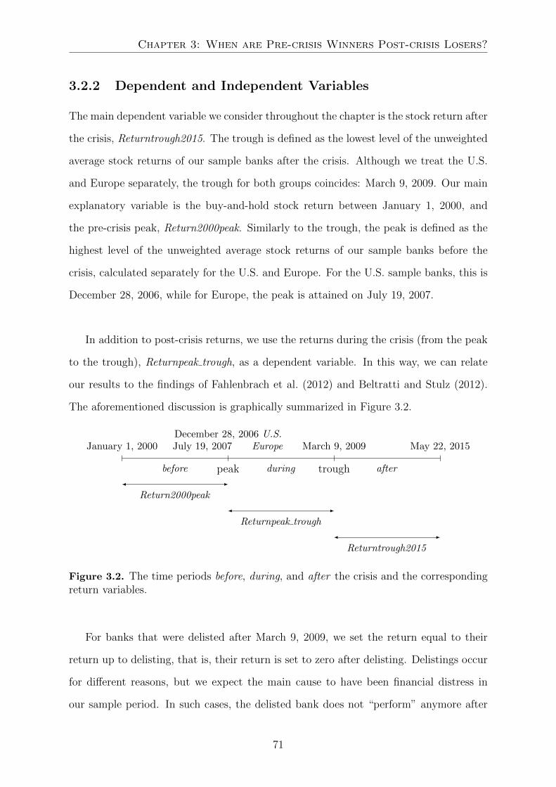
Chapter 3: When are Pre-crisis Winners Post-crisis Losers?
3.2.2 Dependent and Independent Variables
The main dependent variable we consider throughout the chapter is the stock return after
the crisis, Returntrough2015. The trough is defined as the lowest level of the unweighted
average stock returns of our sample banks after the crisis. Although we treat the U.S.
and Europe separately, the trough for both groups coincides: March 9, 2009. Our main
explanatory variable is the buy-and-hold stock return between January 1, 2000, and
the pre-crisis peak, Return2000peak. Similarly to the trough, the peak is defined as the
highest level of the unweighted average stock returns of our sample banks before the
crisis, calculated separately for the U.S. and Europe. For the U.S. sample banks, this is
December 28, 2006, while for Europe, the peak is attained on July 19, 2007.
In addition to post-crisis returns, we use the returns during the crisis (from the peak
to the trough), Returnpeak trough, as a dependent variable. In this way, we can relate
our results to the findings of Fahlenbrach et al. (2012) and Beltratti and Stulz (2012).
The aforementioned discussion is graphically summarized in Figure 3.2.
January 1, 2000
before peak
July 19, 2007 EuropeDecember 28, 2006 U.S.
during trough
March 9, 2009
after
May 22, 2015
Return2000peak
Returnpeak trough
Returntrough2015
Figure 3.2. The time periods before, during, and after the crisis and the correspondingreturn variables.
For banks that were delisted after March 9, 2009, we set the return equal to their
return up to delisting, that is, their return is set to zero after delisting. Delistings occur
for different reasons, but we expect the main cause to have been financial distress in
our sample period. In such cases, the delisted bank does not “perform” anymore after
71

Drivers of Bank Performance and The International Cost of Equity
delisting, which motivates the decision for setting the return at zero. This reasoning is
less applicable for banks that were acquired or taken private, however. To alleviate these
concerns, therefore, we perform robustness tests in Section 3.5.2, where delisted banks
are deleted from the sample altogether or the return of delisted banks as of delisting is
extended with a financial index return.
Bank performance during and after the crisis is obviously related to not only pre-
crisis returns, but also other bank characteristics in general and a bank’s riskiness in
particular. We therefore include as control variables bank characteristics from just be-
fore the crisis that have been shown to be relevant to bank performance and riskiness.
Following Fahlenbrach et al. (2012), we control for beta, size, book-to-market of equity,
and market value of leverage. We estimate beta from a weekly CAPM regression model
from 2003 to 2006. Size is measured by the market capitalization of equity, and we apply
a log transformation to adjust for the positive skewness of the distribution and limit the
impact of very large banks. Book-to-market is the book value of common equity to the
market value of common equity. Finally, we use the market value of leverage, MVLever-
age, as defined in Acharya et al. (2017).4 Berger and Bouwman (2013) have shown a
positive relationship between a bank’s equity ratio (i.e., the inverse of the leverage ratio)
and its performance (measured in terms of probability of survival and market share)
during banking crises. Moreover, for small banks, capital is always positively related
to performance (i.e., not only during banking crises). Beltratti and Stulz (2012) have
corroborated this finding for large international banks during the financial crisis, and
Fahlenbrach et al. (2012) have done so for a sample of U.S. banks. Finally, Cole and
White (2012) have documented greater chances of survival for better capitalized banks.
We include three other variables related to bank performance in our main regressions:
funding fragility, securities, and illiquidity. Funding fragility is the proportion of non-
4In our baseline specification, we rely on the market value of equity instead of the book value tocompute our measure of leverage. Calomiris and Herring (2013) showed the discrepancy between thebook value of equity and the true capital strength of banks before and during the crisis, which ex postturned out to be better reflected by the market value of equity.
72
Chapter 3: When are Pre-crisis Winners Post-crisis Losers?
deposit short-term funding to total short-term funding (including deposits) (Demirguc-
Kunt & Huizinga, 2010). Shleifer and Vishny (2010) demonstrated that banks’ reliance
on nondeposit short-term funding was an important factor in the destabilization of the
banking sector and was associated with higher risk (see also Altunbas et al., 2011), while
Demirguc-Kunt et al. (2013) and Beltratti and Stulz (2012) showed that a higher level of
deposit funding (the flipside of nondeposit short-term funding) was associated positively
with returns during the crisis.
Another criterion we use to gauge the banks’ activities is the proportion of securities
to assets. Since a bank’s balance sheet is mainly composed of securities and loans, this
variable is roughly the complement of loans to assets. Although the trigger of the fi-
nancial crisis was mortgage-backed securities (Brunnermeier, 2009, pp. 82–84), Beltratti
and Stulz (2012) found a negative relationship between loans and crisis stock returns and
Altunbas et al. (2011) documented a positive relationship between loans and riskiness.
The third variable, illiquidity, measures the difficulty a bank might experience in re-
paying short-term liabilities in the event of distress. A high value indicates a high level
of nondeposit short-term liabilities in relation to liquid assets, which can lead to trouble
in refinancing the liabilities when these wholesale funding markets experience distress
(Brunnermeier, 2009). However, surprisingly, Demirguc-Kunt et al. (2013) found a pos-
itive relationship between illiquidity and stock performance during the crisis. This is
ascribed to mortgage-backed securities being classified as liquid assets, which turned out
to be less liquid when the crisis struck, and to the increases in banks’ liquidity provided
by the central banks, which could have been interpreted by markets as a signal of weak-
ness.
In some regressions, leverage is replaced by the Tier 1 Ratio, which then automat-
ically excludes investment banks and government-sponsored entities from the sample
(e.g., Fannie Mae and Freddie Mac for the U.S. and Nationale Bank van Belgie and
73

Drivers of Bank Performance and The International Cost of Equity
Schweizerische Nationalbank for Europe). Beltratti and Stulz (2012) found a negative
relationship between Tier 1 Ratio and stock returns during the crisis, and Altunbas et
al. (2011) have demonstrated a negative relationship between risk and this capital ratio.
Unless stated otherwise, all explanatory variables, except for stock returns, are measured
as of December 31, 2006. A description of all variables can be found in Appendix A.
We obtained data from Bankscope, except for the market capitalization and stock
returns data, for which we used Datastream. For the latter, we used the Total Return
datatype of Datastream, which takes the reinvestment of dividends and stock splits into
account. The data from Bankscope can be linked to that from Datastream using the
International Securities Identification Number (ISIN). In some cases, the Bankscope ISIN
did not match the Datastream ISIN. To ensure correspondence between data from both
databases, we then verified the asset size of the bank found in Datastream with the one
provided by Bankscope.
3.2.3 Summary Statistics
Before we present summary statistics for U.S. and European banks we show the trajec-
tory of stock prices over the period studied. Figure 3.3 is the unweighted average for U.S.
and European banks in our sample from 2000 to 2015 (see Appendix B for modifications
to the stock price data).
74

Chapter 3: When are Pre-crisis Winners Post-crisis Losers?
2000 2001 2002 2003 2004 2005 2006 2007 2008 2009 2010 2011 2012 2013 2014 2015
Time
0
0.5
1
1.5
2
2.5
3
3.5
4
Inde
x le
vel
Stock price index of U.S. and European banks 2000 - 2015(dividends reinvested)
U.S. banksEuropean banks
Figure 3.3. Stock prices, adjusted for reinvestment of dividends and stock splits, for theunweighted index of U.S. banks (thin line) and European banks (thick line) from 2000to 2015. The returns for banks delisted after the trough is set to zero, since Datastreamstops providing data as of that moment.
Although the phases of the trajectories are similar, there are some differences between
U.S. and European banks. First, while U.S. bank stock returns increase continuously
from the start of the sample period to the peak at the end of 2006, the sustained increase
of stock returns at European banks starts three years later, in the first quarter of 2003.5
Second, stock prices of European banks attain their peak more than six months after
U.S. banks, and the increase before the crisis is somewhat larger in Europe (230%) than
in the U.S. (216%). Third, European banks’ stock returns have recovered significantly
better from the crisis than their U.S. counterparts: 162% for Europe versus 139% for
the U.S. Note that the 2011–2012 Eurozone crisis is visible for the European banks, but
not for U.S. banks. Despite those losses, though, European banks have come out of the
financial crisis stronger compared to their transatlantic counterparts.6 Hence, the Euro-
5In the U.S. and in Europe, as of the start of 2003, stock prices increase sharply. We interpret thisusing the psychoanalytic analysis of bubble formation developed by Tuckett (2011): the accelerationof stock returns might have been the result of the spread of the belief in the “phantastic object” (i.e.,mortgage backed securities) to an ever broader group of market participants. This belief ultimately ledto “groupfeel” and herding behavior, that is, widespread exposure to the mortgage market.
6This contradicts the common view that European banks lag behind U.S. banks. In The Economist
75

Drivers of Bank Performance and The International Cost of Equity
zone crisis period, studied by Hoque (2013) and Hoque, Andriosopoulos, Andriosopoulos,
and Douady (2015), was confined to European banks and the associated decline in stock
prices was much smaller than during the financial crisis.
We go on below to present the summary statistics for the main variables used through-
out the chapter. Table 3.2 contains the summary statistics for U.S. banks, followed by
Table 3.3, with those for European banks.
Table 3.2. Sample summary statistics of U.S. banks. Variable definitions can be foundin Appendix A. Accounting variables are measured as of December 31, 2006.
25% 75%Number Min Quantile Median Quantile Max Mean SD
Returntrough2015 354 -1.00 0.14 1.13 2.36 23.52 1.71 2.77Returnpeak trough 354 -1.00 -0.88 -0.69 -0.48 0.27 -0.65 0.27Return2000peak 354 -0.33 0.84 1.60 2.69 40.74 2.16 2.89Book-to-market 352 0.14 0.44 0.56 0.71 184.13 1.21 9.92log[Market cap (in $m)] 352 -1.02 4.70 5.36 6.89 12.52 5.97 1.86Market cap (in $m) 352 0.36 110.43 213.28 986.30 274,296.40 5,315.15 24,322.51Beta 354 -16.64 0.11 0.40 0.87 2.20 0.46 1.03MES 354 -0.03 -0.01 -0.01 -0.00 0.01 -0.01 0.01MVLeverage 352 1.04 6.63 8.46 10.80 2,325.08 17.66 126.95BVLeverage 354 1.14 9.68 11.35 13.20 31.63 11.71 3.53TCE Ratio 354 -0.12 0.06 0.07 0.09 0.84 0.08 0.05Tier 1 Ratio 304 0.06 0.10 0.11 0.13 0.27 0.12 0.03Assets (in $m) 354 500.63 750.99 1,265.99 6,043.90 1,884,318.00 36,103.17 178,354.75Loans 354 0.00 0.61 0.71 0.77 0.92 0.67 0.18Securities 354 0.00 0.11 0.17 0.26 0.89 0.20 0.14Risk weight 299 0.41 0.68 0.77 0.84 1.22 0.76 0.12Customer deposits 354 0.00 0.67 0.74 0.81 0.90 0.70 0.20Funding fragility 352 0.00 0.03 0.07 0.12 1.00 0.13 0.21Illiquidity 354 0.00 0.43 1.23 3.01 48.97 2.34 3.88IV 354 0.02 0.04 0.05 0.07 11.85 0.15 0.70
The median book-to-market ratio of the banks in our sample is 0.56. The market
capitalization equals $213m for the median bank. Median beta equals 0.40, which is
considerably lower than 1. An alternative measure for systematic risk is the marginal
(2017b) the stock price development of the largest U.S. and European banks were compared. Thedifference with the course of our indices is mainly caused by two factors. First, the S&P 500 banksindex and STOXX Europe 600 banks index, that is, the ones used in the The Economist, are composedof 71 and 45 banks, respectively, while we consider 354 U.S. and 218 European banks. Second, we usethe equal weighted average of the banks in our sample, while the well-known indices use the marketcapitalization weighted average. Based on the graph from The Economist, we conclude that largeU.S. banks had more difficulty recovering just after the crisis [potentially related to the major, forcefulrecapitalization of the banks (The Economist, 2017a)], but when the Euro crisis spread, these U.S.banks caught up and outperformed their European counterparts as of the second half of 2011. The sloweconomic recovery and the delayed recognition of bad loans at Europe’s large banks (The Economist,2017a) potentially explains their lagging stock returns as of that period.
76

Chapter 3: When are Pre-crisis Winners Post-crisis Losers?
expected shortfall (MES) of Acharya et al. (2017), which measures a bank’s performance
during the 5% worst days of market performance from 2003 to 2006: the median bank
had a return of -0.51% during those days. We use four capital ratios to gauge the finan-
cial robustness of a bank. Following Acharya et al. (2017), we define the market value of
leverage (MVLeverage) as total assets minus the book value of equity plus the market
value of equity, divided by the market value of equity. Alternatively, we consider the
book value of leverage (BVLeverage), which is the proportion of assets to the book value
of equity. The median bank has a lower market value of leverage (8.46) than book value
of leverage (11.35), which is consistent with a median book-to-market ratio of 0.56.7 The
third capital ratio is the amount of tangible common equity to tangible assets, TCE Ra-
tio, which equals 7.3% for the median bank. The fourth ratio is the amount of regulatory
Tier 1 Capital to risk-weighted assets, the Tier 1 Ratio. For the U.S., the median Tier 1
Ratio equals 11%, which is nearly three times the minimum requirements of Basel I and
II, while the bank with the lowest Tier 1 Ratio, at 6%, still considerably exceeds those
regulatory requirements (the minimum Tier 1 Capital Ratio prescribed in the Basel I and
II Accords was 4%). The median bank has $1.3bn assets, but there is a large variance
in size: the smallest bank in our sample has $501m assets and the largest bank $1,884bn.
The banks in our sample hold many more loans (median of 71%) on their balance
sheet than securities (median of 17%). The risk weights of assets variable for the median
bank equals 77%, that is, every dollar of assets counts for 0.77 dollar in the computation
of the risk-adjusted assets. These risk-adjusted assets are the denominator in the Tier 1
Ratio. On average, 74% of the median balance sheet is funded with customer deposits.
Furthermore, only a small portion of total short-term funding (i.e., including deposits) is
funded with nondeposit funds, such as money-market funds. Hence, the funding fragility
at our median bank is only 7%. A large variance exists in the proportion of liquid assets
for honoring short-term obligations. The illiquidity variable ranges from 0 (no short-term
7A book-to-market ratio of 1 would imply equality between the market and book value of equity andthus equality of the market and book value of leverage. Since the market value of equity is mostly largerthan the book value, the book value of leverage is in most cases larger than the market value.
77

Drivers of Bank Performance and The International Cost of Equity
liabilities) to 48.97 (48.97 dollars of short-term liabilities to every dollar of liquid assets).
An alternative measure of bank risk is the idiosyncratic volatility (IV) of bank returns,
measured by the nonsystematic variability in stock returns.
Finally, we take a closer look at the outliers in our sample. The maximum val-
ues for our main dependent variable, Returntrough2015, and independent variable, Re-
turn2000peak, equal 23.52 and 40.74, respectively. Considering that the medians for
these two variables are 1.13 and 1.60, respectively, these are outliers. Moreover, many
other variables, most notably Book-to-market, MVLeverage, Beta, and Illiquidity, also
have outliers. The sensitivity of OLS estimates to outliers motivates us to check whether
our main results remain valid when we Winsorize the data at the 1% level.
Table 3.3. Sample summary statistics of European banks. Variable definitions can befound in Appendix A. Accounting variables are measured as of December 31, 2006.
25% 75%Number Min Quantile Median Quantile Max Mean SD
Returntrough2015 218 -1.00 0.10 1.01 2.73 13.73 1.69 2.43Returnpeak trough 218 -0.99 -0.78 -0.62 -0.45 0.18 -0.58 0.26Return2000peak 218 -0.83 0.56 1.34 2.55 21.78 2.30 3.11Book-to-market 213 0.14 0.39 0.53 0.91 168.02 1.96 11.75log[Market cap (in ¤m)] 213 2.91 5.93 7.07 8.47 11.98 7.24 1.96Market cap (in ¤m) 213 18.42 375.15 1,176.81 4,791.15 159,906.31 8,507.48 20,328.94Beta 218 -0.26 0.13 0.46 0.80 1.82 0.50 0.43MES 218 -0.04 -0.02 -0.01 -0.00 0.01 -0.01 0.01MVLeverage 213 1.01 5.28 10.54 17.88 1,809.60 28.16 139.18BVLeverage 218 1.02 7.34 12.28 17.84 107.10 14.29 11.71TCE Ratio 218 -0.07 0.05 0.07 0.12 0.98 0.15 0.23Tier 1 Ratio 119 0.06 0.07 0.09 0.11 0.34 0.10 0.05Assets (in ¤m) 218 388.14 2,188.60 7,838.34 40,181.10 1,571,768.00 105,400.03 285,382.52Loans 218 0.00 0.30 0.60 0.75 0.94 0.51 0.29Securities 218 0.00 0.07 0.16 0.31 0.99 0.24 0.25Risk weight 113 0.15 0.50 0.63 0.76 1.33 0.62 0.21Customer deposits 218 0.00 0.19 0.42 0.56 0.89 0.38 0.25Funding fragility 206 0.00 0.11 0.26 0.50 1.00 0.35 0.30Illiquidity 216 0.00 0.27 0.72 1.80 91.26 2.37 7.35IV 218 0.01 0.03 0.04 0.05 0.12 0.04 0.02
In discussing the characteristics of European banks, we focus on the differences with
U.S. banks. First, European banks are much larger on average than U.S. banks: their
median market capitalization is more than seven times higher than that of U.S. banks and
their median asset size more than eight times higher. Second, the median European bank
is funded with only 42% customer deposits, compared to 74% for the median American
78

Chapter 3: When are Pre-crisis Winners Post-crisis Losers?
bank, indicating that the funding fragility of European banks is higher. Third, European
banks also seem more fragile than their American counterparts in terms of capital ratios.
However, one must be cautious when comparing the summary statistics of capital ratios
between the U.S. and Europe because of differences in the accounting standards used.
Financial institutions in the U.S. use Generally Accepted Accounting Principles (U.S.
GAAP), whereas in Europe, the International Financial Reporting Standards (IFRS)
prevail. Admati and Hellwig (2013, pp. 83–85) have pointed out that in the case of JP
Morgan Chase, for example, total assets on December 31, 2006, would have been 79%
higher based on IFRS compared to U.S. GAAP. The main two reasons for such large
differences are that in the U.S. more assets can be removed from the balance sheet and
derivatives of the same counterparty on the assets and liabilities side of the balance sheet
can be cancelled out (so-called netting). The IFRS framework has more restrictions in
these respects.
Supposing the U.S. GAAP versus IFRS difference for JPMorgan Chase were to be
extended to our sample of banks, the IFRS-consistent value of assets would increase by
79%, as well. Correspondingly, the median Tier 1 Ratio of 11.1% of U.S. banks would
decrease to (11.1%/1.79=) 6.2%, which is 2.7 percentage points lower than the 8.9% for
European banks.8 Although it can be expected that JPMorgan Chase holds relatively
more derivatives on its balance sheet and more assets off balance sheet than the average
U.S. bank, it seems reasonable to assume that the median Tier 1 Ratio is not higher in
the U.S. than in Europe. The same holds, mutatis mutandis, for the other capital ratios.
3.3 Results for the U.S.
First, we will discuss the results for the U.S., since that is the focus of our study. We
start by presenting some univariate statistics. This is followed by a discussion of the
regression results.
8We apply the same risk weights used to obtain the U.S. GAAP Tier 1 Ratio to compute the IFRS-consistent Tier 1 Ratio.
79

Drivers of Bank Performance and The International Cost of Equity
3.3.1 Univariate Analysis
Figure 3.3 showed the unweighted average performance of U.S. and European banks from
2000 to 2015. We now take a closer look at the stock returns of U.S. banks by defining
five quintiles based on pre-crisis stock performance, with Quintile 1 containing the 20%
of banks that performed worst pre-crisis and Quintile 5 the 20% of banks that performed
best. Figure 3.4 below depicts the unweighted average stock prices for banks in these
five quintiles for the U.S. Table 3.4 shows the average stock performance before, during,
and after the crisis per quintile.
2000 2001 2002 2003 2004 2005 2006 2007 2008 2009 2010 2011 2012 2013 2014 2015
Time
0
1
2
3
4
5
6
7
Inde
x le
vel
Stock price indexes U.S. banks 2000 - 2015 (dividends reinvested)Quintiles based on pre-crisis performance
Quintile 1Quintile 2Quintile 3Quintile 4Quintile 5
Figure 3.4. U.S. banks’ unweighted average stock prices (adjusted for reinvestment ofdividends and stock splits) per quintile. The first quintile (thinnest line) contains the20% worst performers before the crisis, and the fifth quintile (thickest line) contains the20% best performers.
80

Chapter 3: When are Pre-crisis Winners Post-crisis Losers?
Table 3.4. U.S. banks’ average stock returns per quintile for different time periods.Quintiles are constructed based on pre-crisis stock performance. The first quintile con-tains the 20% worst performers before the crisis, and the fifth quintile contains the 20%best performers.
U.S. Q1 Q2 Q3 Q4 Q5
2000–peak 30% 98% 162% 244% 552%peak–2009 -65% -60% -57% -70% -78%2009–2015 145% 167% 136% 151% 116%
The first line of the table reflects the nature of the quintiles: Quintile 1 contains
the 20% worst performers before the crisis, whereas Quintile 5 contains the 20% best
performers. The difference in pre-crisis performance between the quintiles is considerable,
with the banks in Quintile 5 performing 18 times better on average than those in Quintile
1. During the crisis, the best performers pre-crisis, Quintiles 4 and 5, report the greatest
decline, which is consistent with the findings of Fahlenbrach et al. (2012) and Beltratti
and Stulz (2012). In the post-crisis period, Quintile 5 banks perform worst, whereas
Quintile 2 banks perform best. These univariate results indicate that the banks that
performed best pre-crisis were not only hit hardest during the crisis, but also lagged
behind in the years after the crisis.
3.3.2 Multivariate Analysis
Since the extant literature has documented an impact of certain risk factors on the
performance of banks (see Section 3.2.2), we now want to extend the aforementioned
univariate analysis to a multivariate setting by estimating the following model:
Returntrough2015i = α + βReturn2000peaki + γXi + εi, (3.1)
where i indicates a bank, Returntrough2015 and Return2000peak are the returns after
and before the crisis, respectively, and Xi are the pre-crisis bank characteristics. Our
goal is to analyze how pre-crisis returns are related to post-crisis returns. Under the
boom-and-bust hypothesis, a negative relationship would be expected, whereas the high
81
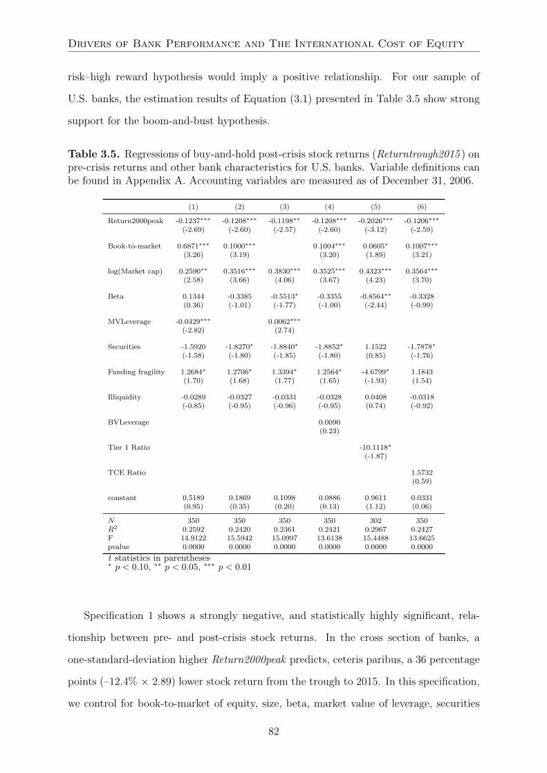
Drivers of Bank Performance and The International Cost of Equity
risk–high reward hypothesis would imply a positive relationship. For our sample of
U.S. banks, the estimation results of Equation (3.1) presented in Table 3.5 show strong
support for the boom-and-bust hypothesis.
Table 3.5. Regressions of buy-and-hold post-crisis stock returns (Returntrough2015 ) onpre-crisis returns and other bank characteristics for U.S. banks. Variable definitions canbe found in Appendix A. Accounting variables are measured as of December 31, 2006.
(1) (2) (3) (4) (5) (6)
Return2000peak -0.1237∗∗∗ -0.1208∗∗∗ -0.1198∗∗ -0.1208∗∗∗ -0.2026∗∗∗ -0.1206∗∗∗
(-2.69) (-2.60) (-2.57) (-2.60) (-3.12) (-2.59)
Book-to-market 0.6871∗∗∗ 0.1000∗∗∗ 0.1004∗∗∗ 0.0605∗ 0.1007∗∗∗
(3.26) (3.19) (3.20) (1.89) (3.21)
log(Market cap) 0.2590∗∗ 0.3516∗∗∗ 0.3830∗∗∗ 0.3525∗∗∗ 0.4323∗∗∗ 0.3564∗∗∗
(2.58) (3.66) (4.06) (3.67) (4.23) (3.70)
Beta 0.1344 -0.3385 -0.5513∗ -0.3355 -0.8564∗∗ -0.3328(0.36) (-1.01) (-1.77) (-1.00) (-2.44) (-0.99)
MVLeverage -0.0429∗∗∗ 0.0062∗∗∗
(-2.82) (2.74)
Securities -1.5920 -1.8270∗ -1.8840∗ -1.8852∗ 1.1522 -1.7878∗
(-1.58) (-1.80) (-1.85) (-1.80) (0.85) (-1.76)
Funding fragility 1.2684∗ 1.2706∗ 1.3394∗ 1.2564∗ -4.6799∗ 1.1843(1.70) (1.68) (1.77) (1.65) (-1.93) (1.54)
Illiquidity -0.0289 -0.0327 -0.0331 -0.0328 0.0408 -0.0318(-0.85) (-0.95) (-0.96) (-0.95) (0.74) (-0.92)
BVLeverage 0.0090(0.23)
Tier 1 Ratio -10.1118∗
(-1.87)
TCE Ratio 1.5732(0.59)
constant 0.5189 0.1869 0.1098 0.0886 0.9611 0.0331(0.95) (0.35) (0.20) (0.13) (1.12) (0.06)
N 350 350 350 350 302 350R2 0.2592 0.2420 0.2361 0.2421 0.2967 0.2427F 14.9122 15.5942 15.0997 13.6138 15.4488 13.6625pvalue 0.0000 0.0000 0.0000 0.0000 0.0000 0.0000
t statistics in parentheses∗ p < 0.10, ∗∗ p < 0.05, ∗∗∗ p < 0.01
Specification 1 shows a strongly negative, and statistically highly significant, rela-
tionship between pre- and post-crisis stock returns. In the cross section of banks, a
one-standard-deviation higher Return2000peak predicts, ceteris paribus, a 36 percentage
points (–12.4% × 2.89) lower stock return from the trough to 2015. In this specification,
we control for book-to-market of equity, size, beta, market value of leverage, securities
82

Chapter 3: When are Pre-crisis Winners Post-crisis Losers?
to assets, funding fragility, and illiquidity of assets. This equals 21% of the sample mean
return of 171% in the post-crisis period. Since Book-to-market and MVLeverage are al-
most perfectly correlated, with a correlation coefficient of 0.9972 and Variance Inflation
Factor (VIF) of over 200, we estimate the model excluding MVLeverage in Specifica-
tion 2 and Book-to-market in Specification 3. Results in Specification 2 are similar to
Specification 1, while MVLeverage flips in sign between Specifications 1 and 3. These
three regressions provide strong support for the boom-and-bust hypothesis and show
that banks that performed well before the crisis performed badly afterwards.
Book-to-market has the expected sign, while the sign for size, log(Market cap), is
opposite to expectations. High systematic risk before the crisis, as measured by Beta,
is negatively associated with performance after the crisis. Moreover, we conclude that
banks that were highly leveraged pre-crisis show relatively strong post-crisis returns.
Banks with lower securities to assets and more nondeposit short-term debt also perform
better in the post-crisis period, although these variables are not always significant, and
when they are, it is only at the 10% level.
In Specifications 4 through 6, MVLeverage has been replaced by three alternative
capital ratios. When it is replaced with BVLeverage (assets divided by the book value
of equity), leverage is no longer significant, while we obtained similar results as in Spec-
ification 1 for the other variables.
Since depository institutions are required to report Tier 1 Ratios, we assess in Speci-
fication 3 how results change when we restrict the sample to these institutions. The main
result becomes stronger than for the cross section of banks: a one-standard-deviation
higher return before the crisis predicts, ceteris paribus, a 42 percentage points (–20.3% ×
2.07) lower return after the crisis. Compared to the other specifications, funding fragility
is now negatively related to post-crisis returns. Depository banks with more nondeposit
short-term funding show relative underperformance after the crisis. Unreported regres-
83

Drivers of Bank Performance and The International Cost of Equity
sions, in which we estimate Specifications 2 and 3 only for depository institutions, show
the same strong negative correlation between pre- and post-crisis returns for depository
institutions. When we restrict the estimation of Specifications 2 and 3 to non-depository
institutions, the pre-crisis returns still have a negative sign but become insignificant.
Taken together, these results indicate that depository institutions drive the overall neg-
ative return between pre- and post-crisis returns. Finally, following Beltratti and Stulz
(2012) and Fahlenbrach et al. (2012), we include the tangible common equity ratio (TCE
Ratio) in Specification 4, which does not alter our main findings.
In discussing the summary statistics, we identified outliers for the dependent and in-
dependent variables. To assess whether the above results were driven by outliers, we re-
peated the analysis on data which had been Winsorized at 1%. Although the significance
of the pre-crisis returns drops, it remains significant at 5% in four of the specifications
and at 10% (with a maximum p-value of 0.053) in the other two. For Specification 1, a
one-standard-deviation higher return before the crisis is associated, ceteris paribus, with
a 29 percentage points lower return after the crisis. Moreover, the negative relationships
for Securities and Illiquidity become stronger, while Funding fragility is insignificant in
Specifications 1 to 4 and 6.
In sum, controlling for bank characteristics, we consistently find support for the
boom-and-bust hypothesis. This significant relationship still holds when we Winsorize
the data at 1%, although the p-values increase slightly. The overall result seems to be
mainly driven by depository institutions, as the relationship between pre- and post-crisis
returns is strongest for these banks.
In order to assess how the results of our sample relate to earlier studies, most notably
Beltratti and Stulz (2012) and Fahlenbrach et al. (2012), we now shift our attention to
the crisis period, 2007–2009. Table 3.6 presents the estimation results of the following
84

Chapter 3: When are Pre-crisis Winners Post-crisis Losers?
model:
Returnpeak troughi = α + βReturn2000peaki + γXi + εi, (3.2)
where i indicates a bank, Returnpeak trough is the return during the crisis, and the
remaining variables are as previously defined.
Table 3.6. Regressions of buy-and-hold stock returns during the crisis (Return-peak trough) on pre-crisis returns and other bank characteristics for U.S. banks. Variabledefinitions can be found in Appendix A. Accounting variables are measured as of De-cember 31, 2006.
(1) (2) (3) (4) (5) (6)
Return2000peak -0.0095∗∗ -0.0094∗∗ -0.0095∗∗ -0.0094∗∗ -0.0155∗∗ -0.0093∗∗
(-2.09) (-2.07) (-2.09) (-2.16) (-2.36) (-2.08)
Book-to-market 0.0062 -0.0148∗∗∗ -0.0155∗∗∗ -0.0179∗∗∗ -0.0144∗∗∗
(0.30) (-4.82) (-5.28) (-5.51) (-4.77)
log(Market cap) -0.0200∗∗ -0.0167∗ -0.0189∗∗ -0.0187∗∗ 0.0060 -0.0139(-2.02) (-1.78) (-2.06) (-2.08) (0.58) (-1.50)
Beta -0.1202∗∗∗ -0.1371∗∗∗ -0.1264∗∗∗ -0.1440∗∗∗ -0.1778∗∗∗ -0.1337∗∗∗
(-3.26) (-4.17) (-4.16) (-4.57) (-5.00) (-4.14)
MVLeverage -0.0015 -0.0011∗∗∗
(-1.02) (-4.92)
Securities 0.5812∗∗∗ 0.5728∗∗∗ 0.5786∗∗∗ 0.7063∗∗∗ 0.6569∗∗∗ 0.5956∗∗∗
(5.84) (5.78) (5.85) (7.22) (4.78) (6.10)
Funding fragility 0.0297 0.0298 0.0303 0.0623 -0.1718 -0.0204(0.40) (0.40) (0.41) (0.88) (-0.70) (-0.28)
Illiquidity 0.0014 0.0013 0.0014 0.0014 0.0004 0.0018(0.42) (0.38) (0.41) (0.43) (0.08) (0.55)
BVLeverage -0.0205∗∗∗
(-5.66)
Tier 1 Ratio 1.4721∗∗∗
(2.69)
TCE Ratio 0.9152∗∗∗
(3.58)
constant -0.5643∗∗∗ -0.5762∗∗∗ -0.5680∗∗∗ -0.3508∗∗∗ -0.8426∗∗∗ -0.6656∗∗∗
(-10.44) (-10.92) (-10.81) (-5.45) (-9.74) (-11.56)
N 350 350 350 350 302 350R2 0.2103 0.2079 0.2100 0.2759 0.2905 0.2365F 11.3480 12.8198 12.9911 16.2436 14.9993 13.2058pvalue 0.0000 0.0000 0.0000 0.0000 0.0000 0.0000
t statistics in parentheses∗ p < 0.10, ∗∗ p < 0.05, ∗∗∗ p < 0.01
Since the period we consider as a dependent variable in these regressions largely over-
laps with the period used in Table II of Fahlenbrach et al. (2012) and Table 4 of Beltratti
85
Drivers of Bank Performance and The International Cost of Equity
and Stulz (2012) (both papers use the stock returns for the period from July 2007 to
December 2008 as a dependent variable), we relate our results to theirs. From the first
line, we can conclude that for all regressions the pre-crisis returns are negatively related
to crisis returns, which is consistent with the findings of Fahlenbrach et al. and Beltratti
and Stulz. Given the high correlation between MVLeverage and Book-to-market, Spec-
ification 2 excludes the former and Specification 3 excludes the latter, and we rely on
both specifications in interpreting the coefficients for these two variables.
The coefficients on Book-to-market, Log(Market cap), and the capital ratios are all
similar to the findings of Fahlenbrach et al. (2012): undervalued stocks perform worse,
smaller banks outperform larger ones, and high pre-crisis leverage is punished during the
crisis. However, the coefficient of Market Beta has the opposite sign of those findings.
Although Fahlenbrach et al. consider a shorter period in computing their dependent
variable and their beta is computed based on returns from 2004 to 2006 (whereas we
start in 2003), the most likely reason for this difference would be the sample of banks.
They consider banks with a minimum of $50m assets, while we use a minimum of $500m.
Moreover, they are more restrictive in allowing a bank to be part of their sample. Fur-
thermore, consistent with Beltratti and Stulz (2012), we found that banks with relatively
more securities performed better during the crisis.9 Unlike Beltratti and Stulz, however,
Funding fragility was insignificant in our sample. Apparently, the importance of funding
fragility for banks around the world (Beltratti & Stulz, 2012) does not apply to our
sample of U.S. banks.
For the U.S., we have presented strong evidence that the pre-crisis stock returns
of banks predict low stock performance after the crisis, controlling for book-to-market,
size, beta, leverage or another capital ratio, securities, fragility of funding, and liquidity.
9We refer to Specification 2 in Panels A and B of Table 4 in Beltratti and Stulz (2012) since the sizeof the banks in those regressions is closest to the size of our banks. Nonetheless, their sample banksare much larger than ours because they consider banks with a minimum of $10bn in assets, while weconsider banks with a minimum of $500m. Moreover, they consider banks from 32 different countries,while in Table 3.5 we only consider U.S. banks.
86

Chapter 3: When are Pre-crisis Winners Post-crisis Losers?
Moreover, the relationship between pre- and post-crisis returns is strongest for deposi-
tory institutions. In all regressions, the coefficient of the primary explanatory variable,
Return2000peak, was highly statistically and economically significant. The relationship
we found for U.S. banks could possibly be explained by a risky business model and cor-
porate culture that generated high pre-crisis stock returns but also prevented the banks
from fundamentally restructuring post-crisis and adjusting to the harsh reality of more
stringent rules and regulations and discriminating clients. In order to test whether high
performers before the crisis were more risky, we relate pre-crisis stock returns to risk
characteristics. We measure these characteristics at the end of 2006 (i.e., the end of the
period for which we want to explain the stock returns), since this is the best reflection of
the state at which a bank entered the financial crisis. We therefore estimate the following
equation:
Return2000peaki = α + γXi + εi, (3.3)
where Xi are the pre-crisis bank characteristics. The results are presented in Table 3.7.
87

Drivers of Bank Performance and The International Cost of Equity
Table 3.7. Regressions of buy-and-hold pre-crisis stock returns (Return2000peak) onbank characteristics for U.S. banks. Variable definitions can be found in Appendix A.Accounting variables are measured as of December 31, 2006 and loan growth is therelative increase (or decrease) in net loans between December 31, 2000 and December31, 2006.
(1) (2) (3) (4) (5) (6) (7)
Book-to-market 0.1182 0.0161 0.0164 -0.2579 0.1198 0.0541 -0.0405(0.48) (0.44) (0.57) (-0.59) (0.48) (0.26) (-0.22)
log(Market cap) -0.1125 -0.0965 0.0660 0.0963 -0.1152 -0.0080 0.1272(-0.95) (-0.86) (0.72) (0.90) (-0.97) (-0.06) (1.44)
Beta 0.1286 0.0461 -0.0073 -0.1821 0.0256 -0.6341∗
(0.29) (0.12) (-0.02) (-0.46) (0.06) (-1.87)
MVLeverage -0.0075 0.0206 -0.0084 -0.0034 0.0001(-0.42) (0.61) (-0.47) (-0.21) (0.01)
Securities -4.2939∗∗∗ -4.3319∗∗∗ -3.6771∗∗∗ -3.8381∗∗∗ -4.1009∗∗∗ -0.7334(-3.70) (-3.63) (-3.07) (-3.38) (-3.54) (-0.78)
Funding fragility 2.8688∗∗∗ 2.8718∗∗∗ -3.8051∗ -5.1153∗∗ 2.9774∗∗∗ -1.7607∗
(3.31) (3.30) (-1.76) (-2.34) (3.47) (-1.80)
Illiquidity 0.0224 0.0217 0.0286 0.0480 0.0215 0.0231 0.0202(0.56) (0.54) (0.58) (0.89) (0.53) (0.58) (0.68)
BVLeverage -0.0008(-0.02)
Tier 1 Ratio 2.4325(0.50)
Risk weights 2.6805∗∗∗
(2.60)
Customer deposits -2.8912∗∗∗
(-2.99)
MES 29.0901(0.92)
IV 0.3996∗
(1.82)
Loan growth 0.9193∗∗∗
(8.14)
constant 3.2112∗∗∗ 3.1635∗∗∗ 2.2735∗∗∗ -0.2678 5.5720∗∗∗ 2.7290∗∗∗ 0.7545(5.18) (4.05) (3.01) (-0.30) (4.86) (4.02) (1.54)
N 350 350 302 297 352 350 254R2 0.0602 0.0598 0.0717 0.0630 0.0544 0.0712 0.2687F 3.1312 3.1049 3.2436 2.7745 2.8287 3.2693 11.2510pvalue 0.0032 0.0035 0.0025 0.0083 0.0070 0.0013 0.0000
t statistics in parentheses∗ p < 0.10, ∗∗ p < 0.05, ∗∗∗ p < 0.01
Specification 1 contains the same variables we considered in previous tables.10 In
10Unlike in the previous regressions, the high correlation between Book-to-market and MVLeveragehas almost no influence on the estimation results. We therefore do not report separate regression resultswhere either of them has been excluded.
88

Chapter 3: When are Pre-crisis Winners Post-crisis Losers?
Specifications 2 to 6, one of the variables from Specification 1 is replaced by an alterna-
tive indicator and, in Specification 7, we have added the loan growth from 2000 to 2006
to the variables used in Specification 1. The results presented in Table 3.7 provide sup-
port for the hypothesis that in the U.S. a risky business model was positively related to
returns before the crisis. Banks with risky practices – such as having few securities and
consequently high risk weights, few customer deposits and consequently high fragility in
funding, and high stock return variability, as measured by idiosyncratic volatility (IV)
– showed significantly higher stock returns. Capital ratios, on the other hand, are not
related to pre-crisis stock returns.
The proportion of assets held in securities is negatively related to pre-crisis returns.
Although in hindsight it might be surprising that banks performing worst before the
crisis had relatively more securities on their balance sheet (since the crisis started with
mortgage-backed securities), they were regarded as less risky by regulators at that time:
their risk weights11 were lower. This can be concluded from the negative, and highly
significant, correlation of -0.6935 between Securities to Assets and Risk Weights. The
flip side is that banks with more loans on the balance sheet had higher risk weights (cor-
relation of 0.6517) and were thus viewed as more risky prior to the crisis. The results of
Regression 4 are consistent with this reasoning, since higher risk weights are associated
with positive pre-crisis returns.
Funding fragility is significantly positively related to pre-crisis performance in several
regressions. This indicates that banks with a larger portion of short-term debt funded
with sources other than customer deposits performed better before the crisis. This find-
ing is substantiated by Specification 5, which shows that a higher level of customer
deposits is negatively associated with returns. This is also in line with the finding of
Demirguc-Kunt and Huizinga (2010) that banks that “rely prominently on attracting
11This is a measure to gauge the overall riskiness of a bank’s assets. These risk weights are used tomultiply the assets in obtaining the denominator for regulatory capital ratios, such as the Tier 1 Ratio:the higher the risk weights, the riskier the assets of a bank.
89

Drivers of Bank Performance and The International Cost of Equity
nondeposit funding are very risky” (p. 626).
As an alternative for Beta, we follow Fahlenbrach et al. (2012) and simultaneously
consider the marginal expected shortfall (MES) as defined in Acharya et al. (2017) and
the idiosyncratic volatility (IV) of Beltratti and Stulz (2012). MES is the average stock
returns of banks on the 5% of trading days from 2003 to 2006 when the S&P 500 had
its lowest returns. IV represents the variability in the stock returns not explained by the
market: a higher value implies greater variability after controlling for market variability.
From the significantly positive relationship between IV and pre-crisis return, we again
conclude that riskier banks (i.e., those with a more volatile trajectory) performed better
before the crisis.
Fahlenbrach et al. (2016) have documented that banks with fast-growing loan portfo-
lios in a three year period have lower stock returns in subsequent years than banks with
slow growing loan portfolios. We wonder whether loan growth might also be a relevant
factor in our analyses. In Specification 7 in Table 3.7, we have added loan growth and
conclude that it is strongly positively related to pre-crisis stock returns. Furthermore,
it is a relatively important characteristic as the R2 jumps to 0.27 from a maximum of
0.07 for the other specifications. Given the strength of this relation (t-statistic of 8.14)
loan growth is a candidate for explaining the negative relationship between pre- and
post-crisis stock returns documented in Table 3.5. In an unreported regression we thus
added loan growth to our main regression (i.e., Specification 1 in Table 3.5). We find
that loan growth is significantly negatively related to post-crisis stock returns (at the
10% level) and, moreover, the negative relationship between pre- and post-crisis stock
returns is no longer significant.
In sum, these results indicate that the high-performing banks from before the crisis
were more risky in various respects. The strongest predictor of pre-crisis stock returns
is the growth in the pre-crisis loan book. Furthermore, when we add this loan growth to
90

Chapter 3: When are Pre-crisis Winners Post-crisis Losers?
our main analysis, the pre-crisis returns are no longer significantly negatively associated
with post-crisis returns. This suggests that fast-growing U.S. banks drive the negative
association between pre- and post-crisis stock returns.
3.3.3 Interpretation of U.S. Results
For U.S. banks, we documented a significantly negative association between returns be-
fore and after the crisis. In line with Fahlenbrach et al. (2012) and Beltratti and Stulz
(2012), we also documented that banks that performed relatively well before the finan-
cial crisis performed poorly during it. We have additionally shown that the pre-crisis
performance of these banks was related to a higher risk profile and stronger loan growth.
In relating pre- and post-crisis returns, we controlled for factors that have been shown
in previous studies to influence bank stock performance and riskiness. Hence, although
some of these risk factors from before the crisis are directly related to the performance
of that period, there is only one factor, pre-crisis loan growth, that seems to drive the
overall negative relationship between pre- and post-crisis returns.
In this section, we discuss several interpretations of these findings. Fahlenbrach et al.
(2012) have claimed that banks tend to persist in their business models and that this led
them to perform badly in both the 1998 crisis and the more recent global financial crisis.
Along similar lines, we argue that the business model of banks that performed badly in
the recent financial crisis has not changed since. The reasons for that are different this
time, however. In spite of the magnitude and impact of the 1998 crisis – Robert Rubin,
then U.S. Secretary of the Treasury, stated that it was “the worst financial crisis in the
last 50 years” – it did not lead to stricter banking oversight. On the contrary, one year
after the crisis, the 1999 Gramm-Leach-Bliley Act [the culmination of a $300 million lob-
bying effort by the banking and financial services industries, according to Stiglitz (2009)]
repealed the two provisions of the Glass-Steagall Act of 1932 that restricted affiliations
between commercial and investment banks. In general, policy makers and regulators
failed to constrain and even induced the risks taken by the financial sector (Barth et al.,
91
Drivers of Bank Performance and The International Cost of Equity
2012, Chapter 4; Calomiris & Haber, 2014, pp. 224, 265–269). Since banking regulation
and supervision were loosened rather than tightened in the years after that 1998 Russian
financial crisis, the pre-crisis business model remained viable and the risk culture of banks
flourished as never before, leading to rapid loan growth paired with low levels of capital.
In the aftermath of the financial crisis of 2007–2009, however, banking regulations and
oversight did change considerably, largely making successful pre-crisis business models
obsolete. The pre-crisis winners were incapable of adapting their business models and
risk culture to the new regulatory and economic reality and have consequently generated
lagging stock returns.
We point to measures taken by the Bank for International Settlements, with Basel
III, and the Financial Stability Board as examples of this increased scrutiny to enhance
the safety of the financial system. In addition to these coordinated supranational ac-
tions, individual countries have imposed new laws and stricter regulation, of which the
Dodd-Frank Act and the Volcker Rule are examples in the U.S.12 One concrete measure
that has received much attention in recent years is the higher liquidity and capital re-
quirements. Baily and Elliott (2014) point to five ways in which capital regulation has
become more stringent since the crisis: requirements for more capital and higher quality
capital, an increase in risk weights for computing regulatory capital ratios, requirements
for more capital for trading positions, and the introduction of a crude leverage ratio in
which assets are unweighted. These measures constrained the banks’ potential of unre-
strained loan growth and forced them to become better capitalized. In addition, they
have proven effective: the Financial Stability Board (2015) has documented an increase
in capital, liquidity, and loss-absorbing capacity at U.S. banks. For instance, Common
Equity Tier 1 Capital, the most stringent form of capital for U.S. banks, has risen from
4.6 percent of risk-weighted assets in the fourth quarter of 2007 to 11.6 percent in the
third quarter of 2013 (Baily & Elliott, 2014).
12See http://www.economist.com/node/21547784 for a discussion of the Dodd-Frank Act. The Vol-cker Rule was based on some parts of Dodd-Frank and intended to restrict commercial banks’ proprietarytrading activities and investments in hedge funds and private equity.
92

Chapter 3: When are Pre-crisis Winners Post-crisis Losers?
Above we have presented evidence which suggests that pre-crisis loan growth accounts
for the negative association between pre- and post-crisis performance. We argue that
this growth was induced by the boom in the mortgage market (e.g., Calomiris, 2009;
Calomiris & Haber, 2014, Chapter 7). Although part of these mortgages were sold
through securitization, the most risky banks kept large sums of high-risk mortgages
on their balance sheet before the crisis (Calomiris & Haber, 2014, pp. 275–277). In
addition to this direct exposure, the shadow banking system also enabled the indirect
exposure to the mortgage market.13 For instance, regular banks set up special purpose
vehicles to off-load assets from their balance sheet, which enabled them to circumvent
capital requirements and earn additional profits (Acharya & Schnabl, 2009; Acharya
et al., 2013). These assets were securitized, and the investors in these vehicles were
provided with a liquidity and credit guarantee from the regular bank to assure a high
credit rating for the securities (Pozsar et al., 2010). That is, if a vehicle experienced
problems with funding or had losses on its securities, the regular banks had to take the
assets back onto their balance sheet. Although these securities were not regarded as risky
before the crisis, at least according to their high credit ratings, they became high risks
during and after the crisis (Beltratti & Stulz, 2012). After the financial crisis, when the
mortgage market normalized and securitization was no longer in fashion or even allowed
(Acharya & Schnabl, 2009, Figure 1; Adrian & Shin, 2009, Figure 4), possibly as a
result of increased regulatory scrutiny (Financial Stability Board, 2015), this curbed the
recovery of banks that depended heavily on these practices. To conclude, we note that
the on-balance sheet growth in risky loans is likely to underestimate the total increase in
the exposure to risky loans, that is, including the indirect exposure through the shadow
banking system.
13Pozsar, Adrian, Ashcraft, and Boesky (2010) produced an overview of this shadow banking systemthat estimates it was equal to roughly $13,000bn at the end of 2006 (cf. the size of the regular U.S.banking sector was equal to $9,000bn in 2006 according to Pozsar et al.).
93
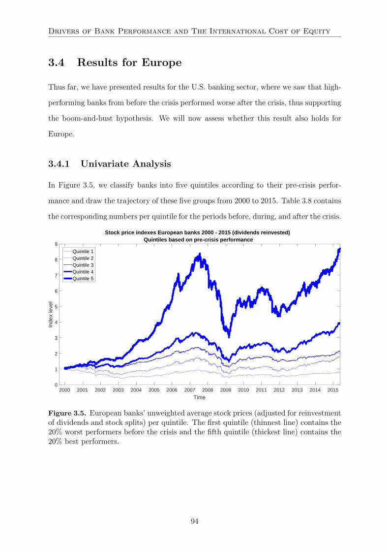
Drivers of Bank Performance and The International Cost of Equity
3.4 Results for Europe
Thus far, we have presented results for the U.S. banking sector, where we saw that high-
performing banks from before the crisis performed worse after the crisis, thus supporting
the boom-and-bust hypothesis. We will now assess whether this result also holds for
Europe.
3.4.1 Univariate Analysis
In Figure 3.5, we classify banks into five quintiles according to their pre-crisis perfor-
mance and draw the trajectory of these five groups from 2000 to 2015. Table 3.8 contains
the corresponding numbers per quintile for the periods before, during, and after the crisis.
2000 2001 2002 2003 2004 2005 2006 2007 2008 2009 2010 2011 2012 2013 2014 2015
Time
0
1
2
3
4
5
6
7
8
9
Inde
x le
vel
Stock price indexes European banks 2000 - 2015 (dividends reinvested)Quintiles based on pre-crisis performance
Quintile 1Quintile 2Quintile 3Quintile 4Quintile 5
Figure 3.5. European banks’ unweighted average stock prices (adjusted for reinvestmentof dividends and stock splits) per quintile. The first quintile (thinnest line) contains the20% worst performers before the crisis and the fifth quintile (thickest line) contains the20% best performers.
94

Chapter 3: When are Pre-crisis Winners Post-crisis Losers?
Table 3.8. European banks’ average stock returns per quintile for different time periods.Quintiles are constructed based on pre-crisis stock performance: the first quintile containsthe 20% worst performers before the crisis, and the fifth quintile contains the 20% bestperformers.
Europe Q1 Q2 Q3 Q4 Q5
2000–peak -6.2% 73% 139% 229% 722%peak–2009 -53% -63% -50% -56% -64%2009–2015 97% 183% 110% 144% 197%
The first line of the table shows that in Europe the worst performers before the
crisis had a negative return of -6.2%, whereas the best performers enjoyed an eight-fold
increase in stock price. During the crisis, the banks in Quintile 5 experienced the greatest
drop, which is in line with our findings for the U.S. However, in a striking difference with
the U.S, the best-performing European banks from before the crisis continue to exhibit
the best performance after the crisis, while the worst performers pre-crisis are again the
worst performers after the crisis.
3.4.2 Multivariate Analysis
We now want to assess the relationship between pre- and post-crisis stock returns when
we control for other bank characteristics. We therefore apply Equation (3.1) to our
European sample. In contrast to the set-up for the U.S., standard errors are now clustered
at the country level. The results are reported in Table 3.9.
95
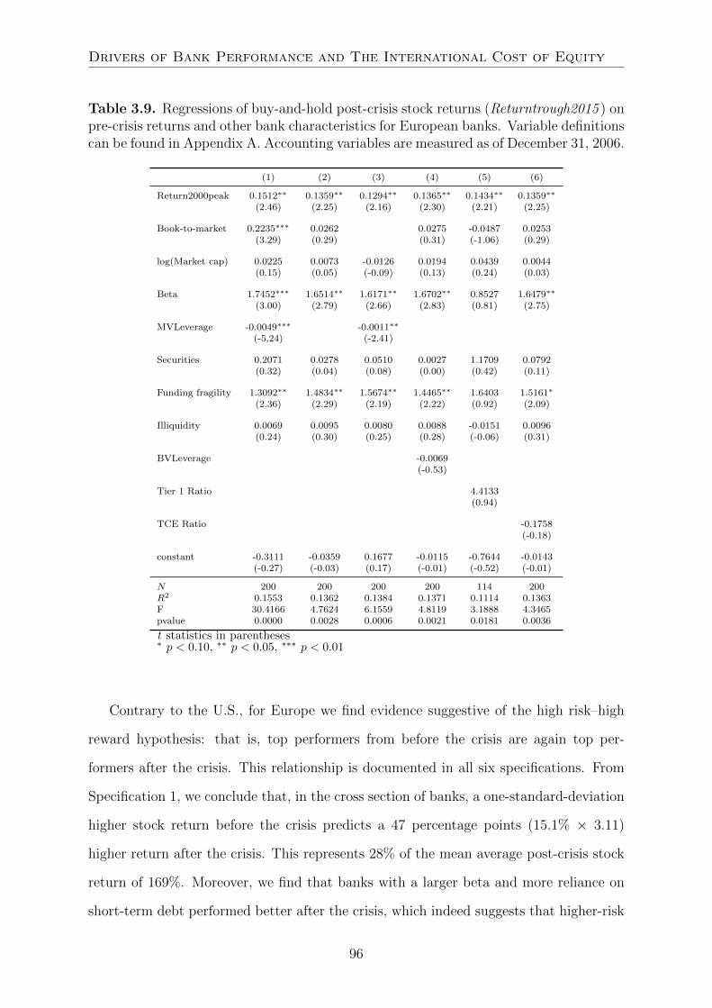
Drivers of Bank Performance and The International Cost of Equity
Table 3.9. Regressions of buy-and-hold post-crisis stock returns (Returntrough2015 ) onpre-crisis returns and other bank characteristics for European banks. Variable definitionscan be found in Appendix A. Accounting variables are measured as of December 31, 2006.
(1) (2) (3) (4) (5) (6)
Return2000peak 0.1512∗∗ 0.1359∗∗ 0.1294∗∗ 0.1365∗∗ 0.1434∗∗ 0.1359∗∗
(2.46) (2.25) (2.16) (2.30) (2.21) (2.25)
Book-to-market 0.2235∗∗∗ 0.0262 0.0275 -0.0487 0.0253(3.29) (0.29) (0.31) (-1.06) (0.29)
log(Market cap) 0.0225 0.0073 -0.0126 0.0194 0.0439 0.0044(0.15) (0.05) (-0.09) (0.13) (0.24) (0.03)
Beta 1.7452∗∗∗ 1.6514∗∗ 1.6171∗∗ 1.6702∗∗ 0.8527 1.6479∗∗
(3.00) (2.79) (2.66) (2.83) (0.81) (2.75)
MVLeverage -0.0049∗∗∗ -0.0011∗∗
(-5.24) (-2.41)
Securities 0.2071 0.0278 0.0510 0.0027 1.1709 0.0792(0.32) (0.04) (0.08) (0.00) (0.42) (0.11)
Funding fragility 1.3092∗∗ 1.4834∗∗ 1.5674∗∗ 1.4465∗∗ 1.6403 1.5161∗
(2.36) (2.29) (2.19) (2.22) (0.92) (2.09)
Illiquidity 0.0069 0.0095 0.0080 0.0088 -0.0151 0.0096(0.24) (0.30) (0.25) (0.28) (-0.06) (0.31)
BVLeverage -0.0069(-0.53)
Tier 1 Ratio 4.4133(0.94)
TCE Ratio -0.1758(-0.18)
constant -0.3111 -0.0359 0.1677 -0.0115 -0.7644 -0.0143(-0.27) (-0.03) (0.17) (-0.01) (-0.52) (-0.01)
N 200 200 200 200 114 200R2 0.1553 0.1362 0.1384 0.1371 0.1114 0.1363F 30.4166 4.7624 6.1559 4.8119 3.1888 4.3465pvalue 0.0000 0.0028 0.0006 0.0021 0.0181 0.0036
t statistics in parentheses∗ p < 0.10, ∗∗ p < 0.05, ∗∗∗ p < 0.01
Contrary to the U.S., for Europe we find evidence suggestive of the high risk–high
reward hypothesis: that is, top performers from before the crisis are again top per-
formers after the crisis. This relationship is documented in all six specifications. From
Specification 1, we conclude that, in the cross section of banks, a one-standard-deviation
higher stock return before the crisis predicts a 47 percentage points (15.1% × 3.11)
higher return after the crisis. This represents 28% of the mean average post-crisis stock
return of 169%. Moreover, we find that banks with a larger beta and more reliance on
short-term debt performed better after the crisis, which indeed suggests that higher-risk
96

Chapter 3: When are Pre-crisis Winners Post-crisis Losers?
banks performed better after the crisis. Restricting the sample to depository institutions
(Specification 5), we find a similar result.
The coefficient on Beta has a positive sign, which is the opposite of what we found
for U.S. banks. Surprisingly, European banks with a larger exposure to the market
performed better after the crisis. Securities to Assets, which was positively related to
Returnpeak2015 in the U.S., is not statistically significant for the European sample.
In order to allow for heterogeneity in the relationship between pre- and post-crisis
returns for GIIPS (Greece, Ireland, Italy, Portugal, and Spain) and non-GIIPS, we inter-
acted the pre-crisis return with a dummy which is equal to one when a bank is located in
a GIIPS country and zero otherwise. In an unreported regression, we found that for non-
GIIPS countries the relationship between pre- and post-crisis returns is similar to the
positive relationship documented in Specification 1 of Table 3.9. For GIIPS countries,
however, the association is negative but insignificant with a p-value of 0.548. We there-
fore conclude that our main result is driven by banks in non-GIIPS countries. Finally, we
also related the performance of European banks during the crisis to performance before
the crisis (unreported). The relationship is negative but insignificant in all specifications.
Hence, pre-crisis top performers recovered significantly stronger from the crisis than
pre-crisis bottom performers and this relationship is driven by banks in non-GIIPS coun-
tries. This positive association between returns before and after the crisis is consistent
with the high risk–high reward hypothesis and contrasts with our finding for U.S. banks.
As we did for the U.S., our next step is then to relate the pre-crisis returns of European
banks to risk characteristics before the crisis. We employ Equation (3.3) and cluster the
standard errors at the country level. Table 3.10 contains the results.
97

Drivers of Bank Performance and The International Cost of Equity
Table 3.10. Regressions of buy-and-hold pre-crisis stock returns (Return2000peak) onbank characteristics for European banks. Variable definitions can be found in AppendixA. Accounting variables are measured as of December 31, 2006 and loan growth is therelative increase (or decrease) in net loans between December 31, 2000 and December31, 2006.
(1) (2) (3) (4) (5) (6) (7)
Book-to-market -0.4295∗∗ -0.1989 -0.1349 -0.5681∗∗ -0.4316∗∗ -0.3800∗∗ -0.3051(-2.74) (-1.67) (-1.65) (-2.44) (-2.78) (-2.80) (-0.68)
log(Market cap) -0.0126 -0.0064 0.0727 -0.0660 -0.0046 -0.0242 -0.2186(-0.10) (-0.05) (0.37) (-0.45) (-0.04) (-0.19) (-1.09)
Beta -1.6073 -1.5410 -3.1658∗∗ -1.7059 -1.9726∗∗ -0.9037(-1.70) (-1.58) (-2.20) (-1.38) (-2.16) (-0.67)
MVLeverage 0.0058∗∗ 0.0080∗∗ 0.0057∗∗ 0.0044∗∗ 0.0016(2.79) (2.17) (2.62) (2.29) (0.23)
Securities -1.9115∗ -1.7033 -0.2678 -1.9069∗∗ -1.6466∗ 0.6130(-1.99) (-1.70) (-0.20) (-2.65) (-1.97) (0.19)
Funding fragility 1.5165 1.3688 3.4080∗∗ 3.6018∗∗ 1.3743 1.8381(1.42) (1.46) (2.28) (2.23) (1.25) (0.69)
Illiquidity 0.0223 0.0202 0.3753 -0.0410 0.0264 0.0250 0.0183(0.81) (0.77) (1.55) (-0.13) (0.99) (0.82) (0.64)
BVLeverage 0.0068(0.13)
Tier 1 Ratio 11.1635(1.48)
Risk weights 4.3028(1.58)
Customer deposits -2.0376∗∗
(-2.15)
MES 77.7426∗∗
(2.24)
IV 19.2908(0.90)
Loan growth 1.8085∗∗
(2.76)
constant 3.4957∗∗ 3.2004∗∗ 1.1204 0.4829 4.9068∗∗∗ 2.6653∗∗ 3.1499∗
(2.78) (2.44) (0.60) (0.33) (3.88) (2.16) (2.01)
N 200 200 114 108 211 200 47R2 0.1058 0.0897 0.2445 0.2556 0.1209 0.1074 0.3756F 2.3482 1.8217 1.6193 4.7389 3.1120 2.8586 664.8555pvalue 0.0635 0.1384 0.1901 0.0032 0.0217 0.0271 0.0000
t statistics in parentheses∗ p < 0.10, ∗∗ p < 0.05, ∗∗∗ p < 0.01
We observe that riskiness at European banks was rewarded before the crisis. First,
high stock returns in that period were associated with high leverage. Moreover, and
similar to in the U.S., banks with little securities to assets and high fragility in funding,
98

Chapter 3: When are Pre-crisis Winners Post-crisis Losers?
and consequently less deposits, and high loan growth performed better before the crisis.
In contrast, banks with large systematic risk performed worse as can be concluded from
the negative sign of Beta and positive sign of MES. Hence, for European banks, we
find some support that higher risk-taking before the crisis was associated with higher
stock returns. Nonetheless, when we add these risk factors to the regression where we
relate pre- to post-crisis stock returns (see Table 3.9), we still find a significant positive
relationship.
3.4.3 Discussion: U.S. Versus Europe
Contrary to the U.S., for Europe we find that the high-performing banks from before the
crisis are also the high-performing banks after the crisis. How can that be explained?
For the U.S., we argued that the banks’ participation in the mortgage bubble, directly
through a growing loan portfolio and indirectly through the shadow banking system,
explains the negative relationship between pre- and post-crisis stock returns. The ben-
efits reaped before the crisis were no longer available after the crisis as a result of the
implosion of the mortgage market and increased regulation, which forced these banks to
adjust their risky business model. In this section, we explore the importance of these
factors for European banks.
First, Barth et al. (2012, Chapter 5) document that the mortgage market of some
European countries, such as Ireland, Spain, and the United Kingdom, also experienced
a boom before the financial crisis. The positive relationship we found between pre-crisis
stock returns and loan growth before the crisis is consistent with this conjecture. Subse-
quently, in an unreported regression we also added loan growth to the main specification
relating pre- and post-crisis stock returns (i.e., Specification 1 of Table 3.9). Although
we found that pre-crisis loan growth is significantly negatively related to stock returns
after the crisis, it does not alter the significant positive association between pre- and
post-crisis returns. In sum, fast-growing European banks had relatively high pre-crisis
and relatively low post-crisis stock returns. Nonetheless, this does not alter the positive
99

Drivers of Bank Performance and The International Cost of Equity
relationship between performance before and after the crisis.
Next, we assess whether European banks were exposed to unobservable risks through
the European shadow banking market. We start with comparing the sizes of the Euro-
pean and U.S. securitization markets. The European securitization market was much
smaller than the U.S. market, peaking at around ¤2,000bn versus a peak in the U.S.
at around $11,000bn (Bank of England and European Central Bank, 2014). Moreover,
the incidence of default on these securities was much lower in Europe than in the U.S.
(Bank of England and European Central Bank, 2014). Therefore, we conclude that it
is unlikely that European banks had large exposures to the European shadow banking
market. Moreover, when they did have a large exposure, the low rate of default restricted
the damage. Hence, the riskiness of the local shadow banking market was considerably
larger in the U.S. than in Europe.
Even though the European shadow banking system was relatively small and stable, a
significant exposure of European banks to the U.S. shadow system might have exposed
them to similar problems as U.S. banks. Pozsar et al. (2010) and Acharya et al. (2013)
have indeed documented such exposure on the part of European banks, but this typically
pertained to the larger financial institutions.14 Moreover, the involvement of these large
European banks in the securitization process was smaller (Pozsar et al., 2010). A possible
explanation for the smaller exposure of European banks relative to their U.S. counter-
parts might be differences in the way various accounting systems treated assets that were
kept off balance sheet. The Bank of England and European Central Bank (2014) have
stated that the U.S. GAAP accounting system was better suited to off-loading assets by
means of structured finance vehicles than the systems applied in Europe (i.e., IFRS or
national GAAP).
14Some relatively small German banks form an exception. The exposed banks had large holdingsof U.S. securities (see http://www.economist.com/news/finance-and-economics/21638143-seven
-german-landesbanken-survived-financial-crisis-are-still and Claessens, DellAriccia, Igan,and Laeven, 2010).
100

Chapter 3: When are Pre-crisis Winners Post-crisis Losers?
The positive association between pre- and post-crisis performance does not disappear
after we control for observable risk factors. Moreover, the exposure of European banks
to the U.S. and European shadow banking systems was only limited. Consequently,
other non-observable factors – that is, factors that are beneficial to bank performance
and did not need to change after the crisis, such as client focus, strong corporate culture,
and quality of management – might explain the positive relationship between pre- and
post-crisis bank performance. If so, the positive association between pre- and post-crisis
performance should merely be regarded as a sign of bank strength and not a reflection
of high risk practices.
3.5 Robustness Checks
In this section, we investigate the robustness of the U.S. results when we apply estimation
techniques to deal with outliers, treat delisted banks differently, use alternative pre-crisis
periods, and focus on different size categories.
3.5.1 Robust Regression
The objectives with robust estimators are to 1) simultaneously maintain a reasonably
high level of efficiency when outliers are absent; 2) remain stable (perform not much
worse) when there are a few outliers; and 3) not break down when there are numer-
ous outliers (Huber & Ronchetti, 2009). Efficiency in our regression context means a
relatively low standard deviation of the regression coefficients. Three types of outliers
are typically identified (e.g., Rousseeuw & Leroy, 2003): vertical outliers, good leverage
points, and bad leverage points. Vertical outliers are observations that are only outliers
in the direction of the dependent variable (y-direction) but not the independent variables
(x-direction). These outliers pull the regression line towards them and can therefore dis-
tort the estimation. Good leverage points are outliers in both the x- and y-directions.
Since they lie close to the regression line, they have no impact on the parameter esti-
mates. Bad leverage points are outlying in the x-direction but not in the y-direction and
101

Drivers of Bank Performance and The International Cost of Equity
hence are not close to the regression line. As the names indicate, good leverage points
are less of a problem than bad leverage points, which distort estimation.
Huber (1964) proposed a generalization to minimize squared residuals and introduced
the M -estimator. The objective is not necessarily to minimize the quadratic error terms,
but to minimize any function. This estimator is referred to as the M -estimator because
this class contains the sample mean, the median, and all the maximum likelihood estima-
tors. Although these estimators are able to deal with vertical outliers, they are unable to
cope with bad leverage points. In other words, they break down when only a few outliers
contaminate the data. Therefore, an alternative class of S-estimators was introduced by
Rousseeuw and Yohai (1984), with which a high breakdown point could be achieved,
meaning that the estimator can handle a relatively large number of outliers before de-
railing. The latter class of estimators, however, suffers from a low level of efficiency
when there are no outliers. Finally, Yohai (1987) developed the MM -estimator, which
has a high breakdown point, while simultaneously enjoying high efficiency. Although this
might seem like the best of both worlds, Huber and Ronchetti (2009) criticize estimators
with a high breakdown point for not being stable; that is, a small number of outliers
might distort the efficiency of the model.
The aforementioned discussion only lists a few of the large number of available robust
estimators15 and indicates that there is no consensus as to which estimator is the pre-
ferred one under which conditions. We therefore list the results for our main regressions
using OLS, Winsorizing at 1%, the M -estimator, and the MM -estimator. We follow
Verardi and Croux (2009) in choosing the rreg command in Stata for our M -estimator
and an efficiency of 70% for our MM -estimator. Results are presented in Tables 3.11
and 3.12.
15See, e.g., Huber and Ronchetti (2009, pg. 195).
102

Chapter 3: When are Pre-crisis Winners Post-crisis Losers?
Table 3.11. Regressions of buy-and-hold post-crisis (Returntrough2015 ) stock returnson pre-crisis returns and other bank characteristics. In Specifications 1 to 3, we use OLS;and in Specifications 4 to 6, we Winsorize the data at 1%. Variable definitions can befound in Appendix A. Accounting variables are measured as of December 31, 2006.
OLS Winsorizing
(1) (2) (3) (4) (5) (6)
Return2000peak -0.1237∗∗∗ -0.1208∗∗∗ -0.1198∗∗ -0.1577∗∗ -0.1483∗ -0.1714∗∗
(-2.69) (-2.60) (-2.57) (-2.07) (-1.95) (-2.28)
Book-to-market 0.6871∗∗∗ 0.1000∗∗∗ 0.8881 1.9695∗∗∗
(3.26) (3.19) (1.08) (3.71)
log(Market cap) 0.2590∗∗ 0.3516∗∗∗ 0.3830∗∗∗ 0.4389∗∗∗ 0.4220∗∗∗ 0.4219∗∗∗
(2.58) (3.66) (4.06) (3.92) (3.77) (3.81)
Beta 0.1344 -0.3385 -0.5513∗ -0.3385 -0.3123 -0.3225(0.36) (-1.01) (-1.77) (-0.81) (-0.75) (-0.77)
MVLeverage -0.0429∗∗∗ 0.0062∗∗∗ 0.0734∗ 0.1084∗∗∗
(-2.82) (2.74) (1.73) (3.95)
Securities -1.5920 -1.8270∗ -1.8840∗ -2.5125∗∗ -2.1902∗∗ -2.6240∗∗
(-1.58) (-1.80) (-1.85) (-2.38) (-2.10) (-2.50)
Funding fragility 1.2684∗ 1.2706∗ 1.3394∗ 1.0074 1.1011 0.9682(1.70) (1.68) (1.77) (1.33) (1.45) (1.28)
Illiquidity -0.0289 -0.0327 -0.0331 -0.0830∗ -0.0750 -0.0812∗
(-0.85) (-0.95) (-0.96) (-1.78) (-1.61) (-1.74)
constant 0.5189 0.1869 0.1098 -1.1399 -1.1152 -0.7936(0.95) (0.35) (0.20) (-1.47) (-1.43) (-1.12)
N 350 350 350 350 350 350R2 0.2592 0.2420 0.2361 0.1143 0.1066 0.1113F 14.9122 15.5942 15.0997 5.5035 5.8270 6.1184pvalue 0.0000 0.0000 0.0000 0.0000 0.0000 0.0000
t statistics in parentheses∗ p < 0.10, ∗∗ p < 0.05, ∗∗∗ p < 0.01
103

Drivers of Bank Performance and The International Cost of Equity
Table 3.12. Regressions of buy-and-hold post-crisis (Returntrough2015 ) stock returnson pre-crisis returns and other bank characteristics. In Specifications 7 to 9, we usethe M -estimator (rreg command in Stata), and in Specifications 10 to 12, the MM -estimator. Variable definitions can be found in Appendix A. Accounting variables aremeasured as of December 31, 2006.
M MM
(7) (8) (9) (10) (11) (12)
Return2000peak -0.0872∗∗∗ -0.0871∗∗∗ -0.0869∗∗∗ -0.2065∗∗∗ -0.2067∗∗∗ -0.1931∗∗∗
(-2.65) (-2.66) (-2.65) (-6.64) (-6.68) (-5.94)
Book-to-market -0.0848 -0.0395 -0.8883 -0.9859∗∗
(-0.23) (-0.70) (-1.53) (-2.54)
log(Market cap) 0.2496∗∗∗ 0.2492∗∗∗ 0.2492∗∗∗ 0.3026∗∗∗ 0.3052∗∗∗ 0.3130∗∗∗
(3.40) (3.40) (3.40) (3.64) (3.76) (3.70)
Beta -0.7357∗∗∗ -0.7324∗∗∗ -0.7297∗∗∗ -1.0691∗∗∗ -1.0843∗∗∗ -0.9496∗∗∗
(-2.63) (-2.63) (-2.62) (-3.65) (-3.94) (-3.28)
MVLeverage 0.0025 -0.0022 -0.0054 -0.0284∗∗∗
(0.12) (-0.69) (-0.31) (-2.83)
Securities 0.6280 0.6386 0.6524 1.9771∗∗∗ 1.9755∗∗∗ 1.9055∗∗∗
(0.87) (0.89) (0.91) (3.13) (3.17) (2.77)
Funding fragility 1.4551∗∗∗ 1.4550∗∗∗ 1.4505∗∗∗ 1.6528∗∗ 1.6526∗∗ 1.5984∗∗
(2.71) (2.72) (2.71) (2.04) (2.06) (1.97)
Illiquidity -0.0211 -0.0211 -0.0210 -0.0076 -0.0081 -0.0112(-0.87) (-0.87) (-0.86) (-0.41) (-0.46) (-0.60)
constant 0.0222 0.0164 0.0078 0.0326 0.0344 -0.3863(0.05) (0.04) (0.02) (0.05) (0.06) (-0.69)
N 349 349 349 350 350 350R2 0.1053 0.1052 0.1048F 5.0016 5.7243 5.7007pvalue 0.0000 0.0000 0.0000
t statistics in parentheses∗ p < 0.10, ∗∗ p < 0.05, ∗∗∗ p < 0.01
First we note that in all 12 specifications, pre-crisis returns remain strongly nega-
tively related to post-crisis returns . Specifications 1, 4, 7, and 10 are the baseline regres-
sions. Due to the high pairwise correlation between MVLeverage and Book-to-market,
we exclude one of these in the other specifications; in interpreting the results for the
Book-to-market and MVLeverage variables, we rely on Specifications 2 and 3. Whereas
significance is comparable when using OLS and the M -estimator, it drops when we Win-
sorize the data and increases considerably when we use the MM -estimator. Applying
the MM -estimator, we find that in the cross section of banks, a one-standard-deviation
higher pre-crisis return predicts a 60 percentage points (–20.7% × 2.89) lower return
after the crisis. This represents a 24 percentage points larger decrease compared to OLS.
104

Chapter 3: When are Pre-crisis Winners Post-crisis Losers?
Comparing the other independent variables, we note that OLS and Winsorizing yield
similar results. However, the M - and MM -estimators do differ for some of the variables.
Although Beta had a negative relationship (not always significant) for OLS and Winsoriz-
ing, it becomes highly negatively significant when using the M - and MM -estimators.
Hence, banks with high systematic risk before the crisis show a significantly lower perfor-
mance in the recovery period. Furthermore, three variables – Book-to-market, MVLever-
age, and Securities – change signs and become significant, at least at the 5% level, with
the MM -estimator. In particular, the highly significant negative sign of MVLeverage is
interesting. When using the MM -estimator, pre-crisis leverage, which is one of the most
prominent risk factors for banks, turns out to be a predictor of post-crisis returns.
Taken all together, though, the negative relationship between pre- and post-crisis
returns remains unchanged when three robust regression alternatives are applied. That
strongly indicates the robustness of our main result. We also performed these robust
regression methods for Europe (unreported). Applying Winsorizing and the M -estimator
raised the positive significant relationship between pre- and post-crisis returns, with
the p-value decreasing from 5% to 1%. However, with the MM -estimator, the p-value
increases to 10%. Hence, for Europe, we also conclude that our main result is consistent
for all specifications.
3.5.2 Delisted Banks
In the main text, we dealt with delisted banks by setting their return equal to zero after
the last day their stock price was recorded in Datastream. In this subsection, we explore
two alternative ways of handling the returns of delisted banks. First, we drop delisted
banks from the sample altogether, and second, we extend the stock returns of delisted
banks with the S&P 500 Financials index as of the moment at which stock data is no
longer available. This latter method was proposed by Fahlenbrach et al. (2012). Table
3.13 contains the results.
105
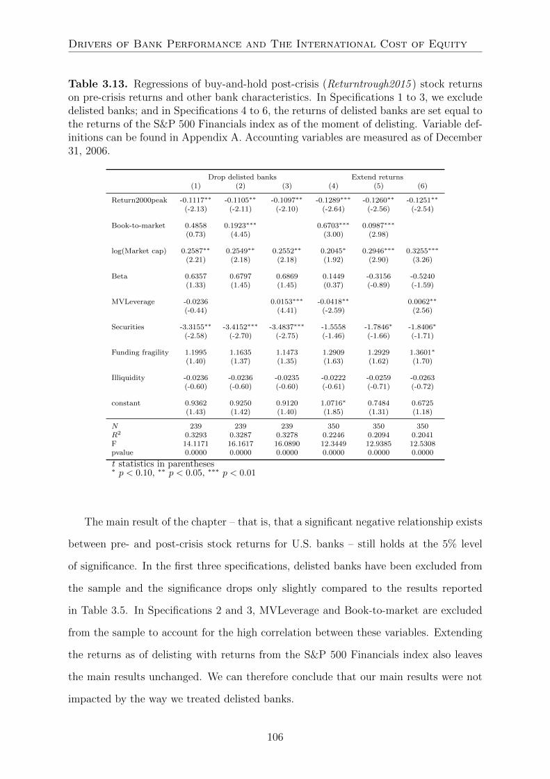
Drivers of Bank Performance and The International Cost of Equity
Table 3.13. Regressions of buy-and-hold post-crisis (Returntrough2015 ) stock returnson pre-crisis returns and other bank characteristics. In Specifications 1 to 3, we excludedelisted banks; and in Specifications 4 to 6, the returns of delisted banks are set equal tothe returns of the S&P 500 Financials index as of the moment of delisting. Variable def-initions can be found in Appendix A. Accounting variables are measured as of December31, 2006.
Drop delisted banks Extend returns(1) (2) (3) (4) (5) (6)
Return2000peak -0.1117∗∗ -0.1105∗∗ -0.1097∗∗ -0.1289∗∗∗ -0.1260∗∗ -0.1251∗∗
(-2.13) (-2.11) (-2.10) (-2.64) (-2.56) (-2.54)
Book-to-market 0.4858 0.1923∗∗∗ 0.6703∗∗∗ 0.0987∗∗∗
(0.73) (4.45) (3.00) (2.98)
log(Market cap) 0.2587∗∗ 0.2549∗∗ 0.2552∗∗ 0.2045∗ 0.2946∗∗∗ 0.3255∗∗∗
(2.21) (2.18) (2.18) (1.92) (2.90) (3.26)
Beta 0.6357 0.6797 0.6869 0.1449 -0.3156 -0.5240(1.33) (1.45) (1.45) (0.37) (-0.89) (-1.59)
MVLeverage -0.0236 0.0153∗∗∗ -0.0418∗∗ 0.0062∗∗
(-0.44) (4.41) (-2.59) (2.56)
Securities -3.3155∗∗ -3.4152∗∗∗ -3.4837∗∗∗ -1.5558 -1.7846∗ -1.8406∗
(-2.58) (-2.70) (-2.75) (-1.46) (-1.66) (-1.71)
Funding fragility 1.1995 1.1635 1.1473 1.2909 1.2929 1.3601∗
(1.40) (1.37) (1.35) (1.63) (1.62) (1.70)
Illiquidity -0.0236 -0.0236 -0.0235 -0.0222 -0.0259 -0.0263(-0.60) (-0.60) (-0.60) (-0.61) (-0.71) (-0.72)
constant 0.9362 0.9250 0.9120 1.0716∗ 0.7484 0.6725(1.43) (1.42) (1.40) (1.85) (1.31) (1.18)
N 239 239 239 350 350 350R2 0.3293 0.3287 0.3278 0.2246 0.2094 0.2041F 14.1171 16.1617 16.0890 12.3449 12.9385 12.5308pvalue 0.0000 0.0000 0.0000 0.0000 0.0000 0.0000
t statistics in parentheses∗ p < 0.10, ∗∗ p < 0.05, ∗∗∗ p < 0.01
The main result of the chapter – that is, that a significant negative relationship exists
between pre- and post-crisis stock returns for U.S. banks – still holds at the 5% level
of significance. In the first three specifications, delisted banks have been excluded from
the sample and the significance drops only slightly compared to the results reported
in Table 3.5. In Specifications 2 and 3, MVLeverage and Book-to-market are excluded
from the sample to account for the high correlation between these variables. Extending
the returns as of delisting with returns from the S&P 500 Financials index also leaves
the main results unchanged. We can therefore conclude that our main results were not
impacted by the way we treated delisted banks.
106
Chapter 3: When are Pre-crisis Winners Post-crisis Losers?
3.5.3 Start of the Pre-crisis Period
Until now we have used January 1, 2000 as starting point to compute the pre-crisis stock
returns. Since this date is chosen rather arbitrarily, in this section, we check for the
robustness of our results when we use two alternative starting points, that is, January
1, 2002 and January 1, 2004. First, in Figure 3.6 we draw graphs for the unweighted
average stock prices per quintile for both starting moments.16
16In this section, we exclude one bank from the sample. Its stock price was equal to 0.20 at the startof 2002 and 0.02 at the start of 2004 while its maximum equaled 28.21 over the period from 2000 to2015. Relative to 0.02 the maximum is 1411 times larger. In addition to these enormous returns, thestock price of this bank can change materially from one day to another, which would distort the graphsof Figure 3.6. Furthermore, the bank’s low stock prices at the start of 2002 and 2004 imply enormouspre-crisis returns, that is, 8000% and 81150%, respectively. Since the bank’s post-crisis stock return isalso an outlier with 2352%, this observation distorts the regression results. Therefore, we exclude it inthis section. We note that this bank did not cause this problem in the main text because its stock pricewas equal to 2.64 on January 1, 2000.
107

Drivers of Bank Performance and The International Cost of Equity
2002 2003 2004 2005 2006 2007 2008 2009 2010 2011 2012 2013 2014 2015
Time
0
0.5
1
1.5
2
2.5
3
3.5
4
4.5
5
Inde
x le
vel
Stock price indexes U.S. banks 2002 - 2015 (dividends reinvested)Quintiles based on pre-crisis performance
Quintile 1Quintile 2Quintile 3Quintile 4Quintile 5
2004 2005 2006 2007 2008 2009 2010 2011 2012 2013 2014 2015
Time
0
0.5
1
1.5
2
2.5
Inde
x le
vel
Stock price indexes U.S. banks 2004 - 2015 (dividends reinvested)Quintiles based on pre-crisis performance
Quintile 1Quintile 2Quintile 3Quintile 4Quintile 5
Figure 3.6. U.S. banks’ unweighted average stock prices (adjusted for reinvestment ofdividends and stock splits) per quintile. The starting dates in the top and bottom panelare January 1, 2002 and January 1, 2004, respectively. The first quintile (thinnest line)contains the 20% worst performers before the crisis, and the fifth quintile (thickest line)contains the 20% best performers.
We conclude that the course of the lines in both the top and bottom figure is largely
similar to the course of the lines in Figure 3.4. Next, in Table 3.14, we present our results
for our main regressions when we apply the alternative starting times.
108

Chapter 3: When are Pre-crisis Winners Post-crisis Losers?
Table 3.14. Regressions of buy-and-hold post-crisis (Returntrough2015 ) stock returnson pre-crisis returns and other bank characteristics. In Specifications 1 to 3, we useJanuary 1, 2002 as starting point for our main independent variable; and in Specifications4 to 6, we use January 1, 2004 as starting point. Variable definitions can be found inAppendix A. Accounting variables are measured as of December 31, 2006.
Start 1-1-2002 Start 1-1-2004(1) (2) (3) (4) (5) (6)
Return2002peak -0.3581∗∗∗ -0.3666∗∗∗ -0.3674∗∗∗
(-3.43) (-3.47) (-3.48)
Return2004peak -0.9796∗∗∗ -1.0208∗∗∗ -1.0172∗∗∗
(-3.32) (-3.42) (-3.41)
Book-to-market 1.5665∗∗∗ -0.0009 1.5460∗∗∗ 0.0109(3.06) (-0.01) (3.01) (0.14)
log(Market cap) 0.3157∗∗∗ 0.3147∗∗∗ 0.3052∗∗∗ 0.3688∗∗∗ 0.3701∗∗∗ 0.3605∗∗∗
(3.11) (3.06) (2.97) (3.59) (3.56) (3.47)
Beta -0.2486 -0.2198 -0.1894 -0.2681 -0.2433 -0.2122(-0.64) (-0.56) (-0.48) (-0.69) (-0.62) (-0.54)
MVLeverage -0.0886∗∗∗ -0.0021 -0.0868∗∗∗ -0.0014(-3.09) (-0.47) (-3.02) (-0.32)
Securities -1.6905∗ -2.0462∗∗ -2.0348∗∗ -1.4741 -1.8276∗ -1.8151∗
(-1.68) (-2.02) (-2.01) (-1.48) (-1.83) (-1.81)
Funding fragility 1.2711∗ 1.0910 1.1046 1.3688∗ 1.2007 1.2111(1.73) (1.47) (1.49) (1.85) (1.61) (1.62)
Illiquidity -0.0341 -0.0380 -0.0375 -0.0508 -0.0554 -0.0549(-1.01) (-1.12) (-1.10) (-1.48) (-1.60) (-1.58)
constant 0.5097 0.7200 0.7800 0.0245 0.2226 0.2809(0.88) (1.24) (1.35) (0.04) (0.41) (0.52)
N 349 349 349 349 349 349R2 0.1206 0.0958 0.0964 0.1187 0.0950 0.0952F 5.8273 5.1635 5.1990 5.7236 5.1124 5.1251pvalue 0.0000 0.0000 0.0000 0.0000 0.0000 0.0000
t statistics in parentheses∗ p < 0.10, ∗∗ p < 0.05, ∗∗∗ p < 0.01
Comparing these results to our main results which we presented in Table 3.5, we
conclude that the negative association between pre- and post-crisis stock returns becomes
stronger when we use two alternative starting points for the pre-crisis period.
3.5.4 Does Size Matter?
One aspect of banks that has been much disputed since the financial crisis is the impor-
tance of their size. Do large banks have specific characteristics – such as, for example,
higher levels of complexity and bureaucracy, a greater lack of transparency, and more
109
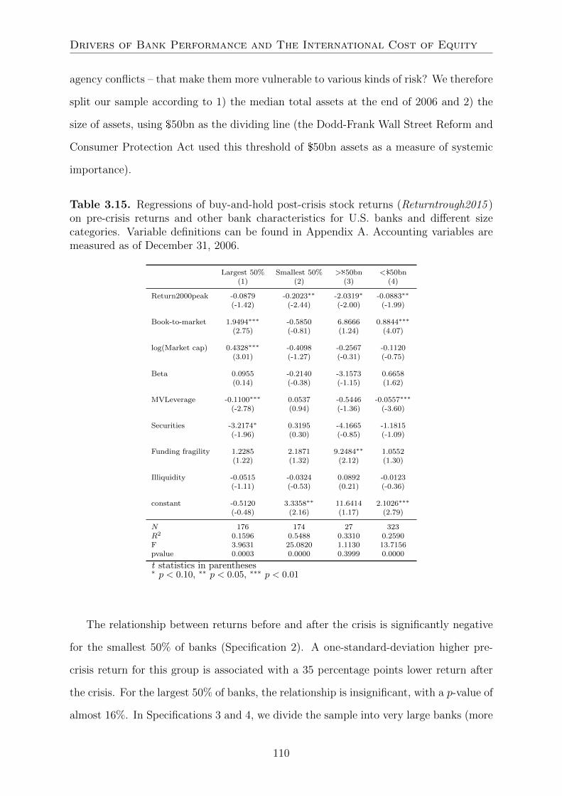
Drivers of Bank Performance and The International Cost of Equity
agency conflicts – that make them more vulnerable to various kinds of risk? We therefore
split our sample according to 1) the median total assets at the end of 2006 and 2) the
size of assets, using $50bn as the dividing line (the Dodd-Frank Wall Street Reform and
Consumer Protection Act used this threshold of $50bn assets as a measure of systemic
importance).
Table 3.15. Regressions of buy-and-hold post-crisis stock returns (Returntrough2015 )on pre-crisis returns and other bank characteristics for U.S. banks and different sizecategories. Variable definitions can be found in Appendix A. Accounting variables aremeasured as of December 31, 2006.
Largest 50% Smallest 50% >$50bn <$50bn(1) (2) (3) (4)
Return2000peak -0.0879 -0.2023∗∗ -2.0319∗ -0.0883∗∗
(-1.42) (-2.44) (-2.00) (-1.99)
Book-to-market 1.9494∗∗∗ -0.5850 6.8666 0.8844∗∗∗
(2.75) (-0.81) (1.24) (4.07)
log(Market cap) 0.4328∗∗∗ -0.4098 -0.2567 -0.1120(3.01) (-1.27) (-0.31) (-0.75)
Beta 0.0955 -0.2140 -3.1573 0.6658(0.14) (-0.38) (-1.15) (1.62)
MVLeverage -0.1100∗∗∗ 0.0537 -0.5446 -0.0557∗∗∗
(-2.78) (0.94) (-1.36) (-3.60)
Securities -3.2174∗ 0.3195 -4.1665 -1.1815(-1.96) (0.30) (-0.85) (-1.09)
Funding fragility 1.2285 2.1871 9.2484∗∗ 1.0552(1.22) (1.32) (2.12) (1.30)
Illiquidity -0.0515 -0.0324 0.0892 -0.0123(-1.11) (-0.53) (0.21) (-0.36)
constant -0.5120 3.3358∗∗ 11.6414 2.1026∗∗∗
(-0.48) (2.16) (1.17) (2.79)
N 176 174 27 323R2 0.1596 0.5488 0.3310 0.2590F 3.9631 25.0820 1.1130 13.7156pvalue 0.0003 0.0000 0.3999 0.0000
t statistics in parentheses∗ p < 0.10, ∗∗ p < 0.05, ∗∗∗ p < 0.01
The relationship between returns before and after the crisis is significantly negative
for the smallest 50% of banks (Specification 2). A one-standard-deviation higher pre-
crisis return for this group is associated with a 35 percentage points lower return after
the crisis. For the largest 50% of banks, the relationship is insignificant, with a p-value of
almost 16%. In Specifications 3 and 4, we divide the sample into very large banks (more
110
Chapter 3: When are Pre-crisis Winners Post-crisis Losers?
than $50bn in assets) and the rest, respectively. We find a significant relationship for
both groups. In the cross section of very large banks, a one-standard-deviation higher
return before the crisis implies a 178 percentage points lower post-crisis return, which
amounts to 44% of the mean return of these banks after the crisis. However, given the
limited sample size of 27 large banks and the inability of rejecting the hypothesis that
all parameter coefficients equal zero (the F -test has a p-value of 0.40), we have to be
careful in drawing firm conclusions from this.
We conclude that the overall negative relationship before and after the crisis is driven
by the smallest 50% of banks and the very large banks. In an unreported regression,
where we focused on the remaining banks – that is, banks in the upper half of the size
distribution with less than $50bn in assets – we found no significant relationship between
pre- and post-crisis returns.
3.6 Summary and Conclusion
We present new, strong evidence that U.S. banks that performed well before the finan-
cial crisis have been unable to recover since because they became bottom performers
in the aftermath of the crisis: high pre-crisis stock returns for U.S. banks predict low
post-crisis stock returns. Moreover, and consistent with earlier studies, we report that
pre-crisis high-performing U.S. banks were bottom performers during the crisis. These
results were not driven by size, type (i.e., investment banks), delistings, or outliers. For
European banks, on the other hand, we found a positive relationship between pre- and
post-crisis stock returns.
High pre-crisis stock returns of U.S. banks were associated with a number of pre-crisis
risk characteristics, notably fragility in funding, a higher variability in stock returns, and
loan growth. This result also holds for European banks, where also high leverage was
positively related with pre-crisis stock returns.
111

Drivers of Bank Performance and The International Cost of Equity
For the U.S., the boom-and-bust hypothesis is strongly supported by our findings.
The analysis indicates that high pre-crisis stock returns were caused by risky business
model characteristics, which seems to be best captured by significant pre-crisis loan
growth. Their low stock returns during the crisis were the negative result of that same
risky business model. We argue that the subsequent underperformance of these pre-
viously high-performing banks in the first six years after the crisis has been due to
the tightening of banking regulations and curbing of risky bank practices that have
largely made the high-risk, high-performing business model from before the crisis obso-
lete. Apparently, the risky business model and practices of pre-crisis high-performing
banks were so deeply engrained in their culture and behavioral and organizational DNA
that they were unable to expeditiously embrace and adopt a new, more client centric,
and trust-based business model. European pre-crisis high-performing banks continued
to systematically outperform after the crisis. Unlike their U.S. counterparts, these banks
experienced less trouble in adjusting to the post-crisis environment.
Appendix
A. Variable Definitions
� Assets - We use the $ book value of assets for U.S. banks and the ¤ book value
for European banks (in millions).
� Beta - Beta of CAPM is used as a proxy for systematic risk. For American com-
panies, we estimate a CAPM of weekly returns in excess of the three-month T-bill
from January 1, 2003, to December 31, 2006. The market is represented by the
S&P 500 index. For European banks, we use the euro interbank lending rate for
three months (i.e., Euribor) as the short rate and the STOXX 600 as the index.
We estimate the following time series regression:
Ri,t − r0,t = αi + βi (RM,t − r0,t) + εi,t, (3.4)
112

Chapter 3: When are Pre-crisis Winners Post-crisis Losers?
where Ri,t is the return of company i in week t, r0,t the short rate, and RM,t the
market return. βi is the exposure to systematic risk of company i and the variable
in question.
� Book-to-market - Book value of common equity to market value of common equity.
� BVLeverage - The book value of assets to book value of equity. The book value of
equity is the sum of equity and preferred shares and hybrid capital accounted for
as equity.
� Customer deposits to assets - Customer deposits to total assets.
� Funding fragility - Deposits from other banks, other deposits, and short-term bor-
rowings, and repurchase agreements and cash collateral normalized by total de-
posits (customers and companies), money market funds, and short-term funding.
� Illiquidity - Deposits from other banks, other deposits, and short-term borrowings,
and repurchase agreements and cash collateral normalized by liquid assets.
� IV - Idiosyncratic volatility defined as
IVi =√
Var (ei,t), (3.5)
where ei,t is the residual for company i at time t from the CAPM regression [see
regression Equation (3.4)].
� Loans - Net loans to assets. Net loans equals gross loans minus the reserves for
impaired or non-performing loans.
� Loan growth - The relative increase (or decrease) in net loans between December
31, 2000 and December 31, 2006.
� Market capitalization - The market value of equity in $ millions for U.S. banks and
¤ millions for European banks. The maximum for Datastream’s Market Value
(MV) and Market Value for Company (MVC) variables is used. For companies
with a single listed equity security, these numbers are equal. For companies with
113

Drivers of Bank Performance and The International Cost of Equity
more than one listed equity security or unlisted equity securities, the latter is the
sum of these, while the former ignores them.
� MES - Marginal Expected Shortfall from Acharya et al. (2017). The average return
of company i during the 5% worst daily market returns between January 1, 2003,
and December 31, 2006:
MESi,5% =1
#days
∑t: market return is in 5% tail
Ri,t, (3.6)
where Ri,t is the return of company i during day t.
� MVLeverage - The book value of assets minus the book value of equity (see
BVLeverage for definition) plus the Market capitalization normalized by Market
capitalization.
� Return2000peak - Buy-and-hold stock returns, with reinvested dividends and ad-
justed for stock splits, from January 1, 2000, to the pre-crisis peak. The peak is
defined as the highest level of the unweighted average of buy-and-hold stock re-
turns for our sample banks before the start of the crisis. In the U.S., the peak was
reached on December 28, 2006, and in Europe, on July 19, 2007.
� Returnpeak trough - Buy-and-hold stock returns, with reinvested dividends and
adjusted for stock splits, from the peak to the trough. The peak is defined as
the highest level of the unweighted average of buy-and-hold stock returns for our
sample banks before the start of the crisis. In the U.S., the peak was reached on
December 28, 2006, and in Europe, on July 19, 2007. The trough is the lowest level
of the unweighted average of buy-and-hold stock returns for our sample banks after
the start of the crisis. This date, March 9, 2009, coincides for U.S. and European
banks.
� Returntrough2015 - Buy-and-hold stock returns, with reinvested dividends and
adjusted for stock splits, from the trough to May 22, 2015. The trough is the
lowest level of the unweighted average of buy-and-hold stock returns for our sample
114

Chapter 3: When are Pre-crisis Winners Post-crisis Losers?
banks after the start of the crisis. This date, March 9, 2009, coincides for U.S.
and European banks. The returns for banks delisted after the start of the crisis
are set equal to zero as of the moment their stock price is no longer available in
Datastream.
� Risk weight - The bank’s risk weight according to the Basel rules and computed
as the risk-weighted assets to assets. For banks for which risk-weighted assets are
not available, we can sometimes use:
Tier 1 CapitalTier 1 Ratio
Assets=
Risk-weighted assets
Assets.
� Securities - Securities held on the balance sheet to total assets. The securities
category is comprised of reverse repurchase agreements, cash collateral, trading
securities, derivatives, available for sale securities, held to maturity securities, at-
equity investments, and other securities.
� TCE Ratio - Tangible common equity to tangible assets. Goodwill and other
intangibles are subtracted from common equity to obtain the numerator and from
assets to obtain the denominator.
� Tier 1 Ratio - The ratio of Tier 1 Capital to risk-weighted assets.
B. Manual Data Adjustments
Certain firms had a stock price (Return Index in Datastream) equal to zero. However,
in some cases, the stock price then grew larger than zero. Since the stock returns would
otherwise be equal to infinity for stocks that recover to values greater than zero, the
zeros have been replaced with the first non-zero stock price after the zeros. So if a stock
price is non-zero at t = 0 and t = 2 and equal to zero at t = 1, the price of t = 2 is used
as the price at t = 1. This occurred in ten cases in our dataset.
115

Drivers of Bank Performance and The International Cost of Equity
116

4 | There’s a New Sheriff in Town:
The Case of a Cooperative Bank
Co-Authors: Kees Cools, Hans Groeneveld, and Arthur van
Soest
Abstract
How does CEO turnover impact bank performance? To answer this question,
we use a panel data set with information on 106 banks over a 5-year period
(2010–2015). This sample provides a unique setting for testing whether and
how CEO turnover matters for bank performance by balancing homogeneity
(all banks were part of a single European cooperative) and heterogeneity (the
decision freedom of bank CEOs). We present strong evidence that the return
on assets significantly declines in the first year(s) after a CEO change. Eco-
nomically, the effect is large, with declines of 0.08 percentage points in the first
year and 0.17 percentage points in the first two years, amounting to 23% and
50% of the standard deviation in return on assets, respectively. The decline in
performance is caused almost entirely by an increase in provisions for impaired
loans. The evidence points to two underlying motives for this increase: 1) to
offset a backlog in provisions on the part of the old CEO and 2) to ensure a po-
sition from which to boost results in the future through a subsequent decrease
in provisions.
117

Drivers of Bank Performance and The International Cost of Equity
4.1 Introduction
We investigate how the performance of a cooperative bank is influenced by a change in
CEO. Research on the impact of CEOs on firm policies and performance has increased
in recent years. Bertrand and Schoar (2003) have highlighted the importance of CEO
styles for investment, financial, and organizational decisions in industrial firms. Focus-
ing on specific attributes, Graham et al. (2013) showed that optimistic CEOs fund their
balance sheet with more debt, in particular short-term debt, and that the risk tolerance
of a CEO is positively related to acquisitions. Another attribute that has received ample
attention in this literature is the impact of overconfidence on the part of CEOs on firm
policies and performance. In a seminal paper, Roll (1986) showed how hubris among
CEOs explains why bidding firms pay too much for their targets. Malmendier and Tate
(2005) elucidated that overconfident CEOs overestimate the returns of their investment
when there is enough internal capital available. They also showed that overconfident
CEOs underinvest when they need to issue equity to fund investments, since they regard
their company’s stock as being undervalued. In addition, building on Roll, Malmendier
and Tate (2008) showed that overconfident CEOs pay too much for target companies and
engage in value-reducing mergers. The aforementioned studies all concerned industrial
firms; meanwhile Ho, Huang, Lin, and Yen (2016) applied the overconfidence measure
to the U.S. banking sector prior to the financial crisis. Banks with CEOs that exhib-
ited overconfidence expanded their loan portfolios (especially in real estate loans) more
aggressively than those with non-overconfident CEOs. This, in turn, led to greater loan
losses and lagging operating and stock performance when the crisis unfolded.
Although these studies are just the tip of the iceberg, they illustrate the importance
of CEO characteristics for firm policies, riskiness, and performance. Given this influence,
instances of a change in CEO provide ample opportunity for further analyzing the impact
of the person at the top. In this chapter we investigate the impact of CEO turnover at lo-
cal banks that are members of a single cooperative organization in Europe. These banks
118

Chapter 4: There’s a New Sheriff in Town
enjoy a high degree of autonomy, which enables their CEOs to influence their financial
performance. We investigate this impact of the CEO around the time of a CEO change.
Our evidence shows that, in a new CEO’s first year, the financial performance of the bank
declines significantly. Since the banks we studied are not listed, financial performance is
measured by return on assets (i.e., net earnings divided by assets), similar to Demirguc-
Kunt and Huizinga (2001) and Iannotta, Nocera, and Sironi (2007). The drop in return
on assets equaled 0.08 percentage points, which was also economically large, representing
23% of the return on assets’ standard deviation. When we included a lagged effect in the
second year, the total decline over the first two years increased to 0.17 percentage points.
This decline seems not to have been caused by a difference in quality1 between the
exiting and incoming CEO, since the decline in performance is observed independent of
the reason for a predecessor’s departure. If the overall decline were attributable to qual-
ity differences between the CEOs, then the successors of CEOs who were being promoted
(an act that testifies to their high quality) would be expected to show the largest decline
in performance in the group. Yet, the opposite is true: the decline in performance is
smallest for banks where a CEO has left as a result of a promotion. Nor does an alter-
native interpretation that new CEOs need time to adjust to their new bank explain the
result, since we observed no material impact on operating performance (i.e., operating
income minus operating costs).
By replacing the return on assets (dependent variable) with the change in loan loss
provisions, we observe that the decline in the former in the first year after a change
of CEO is caused almost entirely by an increase in the latter. This result can be in-
terpreted in two ways: 1) the predecessor had been too lenient in taking provisions for
non-performing loans and correction was needed or 2) the new CEO is taking an earnings
bath. The results point to a combination of both effects, since provisions significantly
decrease – in amounts similar to the increase in the successor’s first year – during the
1Quality should be interpreted as the attributes that are relevant for leading a local bank, cf. Jenter,Matveyev, and Roth (2016).
119

Drivers of Bank Performance and The International Cost of Equity
second-to-last year of the predecessor and the third year of the successor. The decrease in
provisions in the second case also makes it improbable that successors are more cautious
than their predecessors, since it cannot be regarded as prudent to completely deplete the
buffer in provisions two years after it has been built up.
Classifying loans as impaired is not without consequences. Since increases in im-
pairments negatively affect a bank’s capital position, such an action inhibits its room to
provide credit to customers, especially in an environment with increasing capital require-
ments. In addition to this indirect effect on the economy, it also has a direct impact on
clients and the bank itself. If a loan is classified as impaired, the bank puts the borrower
under increased scrutiny, resulting in additional costs for the client and the bank. For
instance, borrowers need to provide a plan to ensure minimal losses for the bank, while
the bank needs to assess the plan’s viability.
We used data for our analysis obtained from the cooperative bank under study,
LinkedIn, and the national statistics bureau. The cooperative provided data on its bal-
ance sheet, income statement, number of members, and market share per bank for the
period from 2010 to 2015. By enriching this data with information from the LinkedIn
profiles of the CEOs, we were able to identify who was CEO at which bank at what time.
Moreover, we have data on the reason for the CEOs’ departures. Finally, to control for
regional differences, we used data on local GDP from the national statistics bureau.
This chapter is related to three streams of the literature. The first is the literature
on the impact of CEO turnover on firm value and performance. Jenter et al. (2016) fo-
cused on the impact of sudden CEO deaths on stock prices to assess whether incumbent
CEOs are valuable to firms. The authors documented great heterogeneity in stock price
reactions to sudden deaths. Overall, the stock price declines, which is consistent with
the incumbent CEO being of value to the firm (Gabaix & Landier, 2008; Tervio, 2008).
However, sudden deaths of older CEOs are associated with positive returns, which is not
120

Chapter 4: There’s a New Sheriff in Town
in line with the theoretical predictions of Gabaix and Landier (2008) and Tervio (2008)
and indicates that firm value can increase after CEO departures. More relevant to our
setting is that Jenter et al. found no impact of CEO death on operating performance
or profits. This contradicts the finding of Bennedsen, Perez-Gonzalez, and Wolfenzon
(2006), however, who documented a decline in operating profitability for private enter-
prises after a CEO dies.
When a CEO dies, the reason for departure is undisputed, and this provides a clean
setting for measuring the impact of the newly appointed CEO on firm value and per-
formance. Other reasons for CEO departure, especially dismissal, have also received
much attention in the literature. The forced departure of CEOs has been used to study
board effectiveness and board monitoring of the CEO. Three important factors related
to this type of CEO departure are firm, industry, and market performance. Jenter and
Lewellen (2010) showed that the probability of a dismissal is significantly higher after
poor firm performance, while Jenter and Kanaan (2015) documented that downturns in
industry and market performance increase the likelihood of dismissal. We contribute to
this strain of the literature by relating the cause of CEO departure to bank performance
in the final year of tenure.
A subfield of the CEO turnover literature is concerned with earnings management
around a CEO change. This is the second stream of literature we relate to. An early
example of this is Moore (1973), who documented larger income-reducing adjustments
– a tactic at the discretion of the CEO – in firms experiencing management changes
than in firms without personnel changes. Strong and Meyer (1987) and Pourciau (1993)
corroborated this result, with the latter focusing exclusively on unanticipated changes in
CEO, and found a reversal in performance in the second year after the change. Most of
these studies do not single out a particular industry. An exception is Bornemann, Kick,
Pfingsten, and Schertler (2015), who focused exclusively on German savings banks. The
authors documented significant increases in discretionary expenses in the first year of a
121

Drivers of Bank Performance and The International Cost of Equity
new CEO. This increase in overall discretionary expenses comprised two opposing forces:
an increase in provisions for loan losses and a decrease in reserves for general bank risks.
Furthermore, they found that new CEOs hired from outside the bank incurred larger dis-
cretionary expenses than those from inside the bank, which is consistent with the results
of Strong and Meyer. Finally, the increase in discretionary expenses can be explained
not only by a need to clean up a bank poorly managed by the predecessor, but also by
the new CEO taking an earnings bath.
This chapter is related to Bornemann et al. (2015) but differs in several respects.
First, Bornemann et al. concentrated exclusively on earnings manipulation on the part
of the new CEO, whereas we focus on the overall performance of the bank in terms of
return on assets. We found that changes in return on assets in the CEO’s first year can
almost entirely be attributed to changes in loan loss provisions. Second, we extend the
analysis by also considering the performance of departing CEOs in the last years before
leaving and the performance of new CEOs after their first year. Third, Bornemann et
al. focus on savings banks that are owned by cities,2 whereas we consider 106 banks that
are privately-owned by their members and part of one cooperative organization.
The third stream of literature to which we contribute is research on bank perfor-
mance. Since the banks we studied are non-listed, we relied on their profitability to
assess performance. We discuss several papers that also use return on assets as a de-
pendent variable. Kok, More, and Pancaro (2015) conducted a recent study on the
performance of European banks that suggests that low GDP growth is the main factor
hampering bank profitability. Demirguc-Kunt and Huizinga (1999) focused on the influ-
ence of market structure on profitability and documented that a higher ratio of banking
assets to GDP and lower market concentration curb profitability. Approaching bank
earnings from a corporate governance perspective, Iannotta et al. (2007) concluded that
2As of June 1, 2016, there were 409 savings banks, of which six were not owned by a city or multi-ple cities; see https://www.dsgv.de/en/facts/facts-and-figures.html and http://www.verband
-freier-sparkassen.de/en/.
122

Chapter 4: There’s a New Sheriff in Town
ownership structure matters, since mutual and government-owned banks perform worse
than their private counterparts. Typically, the samples in these studies are composed of
different types of banks (i.e., commercial, cooperative, and savings banks) from multiple
countries. They must control for many variables in order to measure the impact of the
variable of interest on the performance of the bank. Since the banks in our sample are
all part of the same cooperative organization within one country, we have a unique set-
ting for identifying the drivers of bank performance, in general, and the impact of CEO
turnover on performance, in particular.
The remainder of this chapter is structured as follows. In Section 4.2, we describe the
structure of the cooperative bank. In Section 4.3, we provide a description of the vari-
ables. In Sections 4.4 and 4.5, we discuss the data and summary statistics, respectively.
Finally, Section 4.6 presents the results, and Section 4.7 concludes.
4.2 The Structure of the Cooperative Bank
A stylized overview of the structure of the cooperative bank we studied is provided in
Figure 4.1.
We will work from the bottom to the top in discussing the financial cooperative’s
structure. The blocks at the bottom of the figure represent the local banks. Each local
bank has an independent banking license and a governance structure composed of a Lo-
cal Board of Directors (LBD), a Local Supervisory Board (LSB), and a Local Member
Council (LMC). Separation between the LBD and the LSB is in accordance with the
two-tier corporate governance system common in many European countries. The LBD
manages the bank; its members are appointed by the LSB with the approval of the
central institution. For its part, the LSB advises the LBD and monitors and assesses
its performance within the context of collectively agreed principles and strategies. It
also acts as the employer of the members of the LBD and thereby has the authority
to appoint, suspend, and dismiss individual members in consultation with the central
123
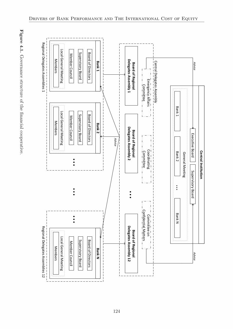
Drivers of Bank Performance and The International Cost of Equity
Bo
ard o
f Directors
Supervisory Bo
ard
Mem
ber C
oun
cil
Local General M
eeting
Bank 1
...
Executive Bo
ardSu
pervisory Board
Ban
k 1
General M
eeting
Ce
ntra
l Institu
tion
Ban
k 2B
ank N
...
Bo
ard o
f Directors
Supervisory Bo
ard
Mem
ber C
oun
cil
Bank 2
Board
of D
irectors
Supervisory Bo
ard
Mem
ber C
oun
cil
Bank N
......
Region
al Delegates A
ssemblies 1
Re
gion
al Delegates A
ssemb
lies 12
Bo
ard o
f Regio
nal D
elegates Assem
bly 1
Cen
tral Delegates A
ssemb
ly
Mem
bers
Mem
bers
Local General M
eeting
Local G
en
eral M
eeting
Mem
bers
Co
mm
ittee o
nC
onfid
ential M
attersC
oordinating
Co
mm
itteeEm
ergency Affairs
Com
mittee
...B
oard
of R
egio
nal D
elegates Assem
bly 12
Bo
ard o
f Regio
nal D
elegates Assem
bly 2
Advice
Advice
Advice
Figure
4.1.
Govern
ance
structu
reof
the
finan
cialco
operative.
124

Chapter 4: There’s a New Sheriff in Town
institution. The LMC consists of 30 to 50 elected members from the local banks. It
appoints, in consultation with the central institution, the members of the LSB, adopts
the financial statements, and decides how money reserved for the local community is
spent. Other members of the bank who are not part of the LMC can have a say in
pivotal decisions through the Local General Meeting.
The central institution of the financial cooperative plays a more supervisory and
accommodating role. In addition to its involvement in nominating, appointing, and dis-
missing members of the two local boards for each bank, it develops financial products,
sets policies (e.g., on human resources and security), and provides access to the financial
markets for local banks. Nonetheless, local banks operate largely independently of the
central institution in their day-to-day business, deciding such matters as which clients to
take on, company loan rates, bank strategy, marketing, and personnel (hiring and firing)
for themselves. Conversely, the local banks can also exert influence on the workings of
the central institution. This occurs through the auspices of the Central Delegates As-
sembly (CDA) (see the middle level in Figure 4.1). The local banks are organized into
multiple Regional Delegates Assemblies, the boards of which make up the representa-
tives of the greater CDA. The CDA is regarded as the “parliament” of the cooperative
and endowed with two main tasks: 1) providing advice to the local banks, the Executive
Board of the Central Institution, and the Local General Meeting for all of the banks and
2) adopting rules for the local banks and approving the budgets granted to them by the
central institution.
Finally, the central institution (see the top level of Figure 4.1) is in its turn governed
similarly to the local banks. It is composed of an Executive Board, a Supervisory Board,
and a General Meeting. The Executive Board is comparable to the LBD on the local
bank level, but now responsible for the entire group. The Supervisory Board has the task
of monitoring the Executive Board. The General Meeting, in which all local banks are
represented, resembles the LMC. It is responsible for adopting the consolidated financial
125

Drivers of Bank Performance and The International Cost of Equity
statements, as well as discharging the Executive and Supervisory Boards.3
The position of local banks within the overall organization provides for an interest-
ing balance between homogeneity and heterogeneity in our sample. Since all of the local
banks are part of one organization, the sample is homogeneous, but the fact that they
have relatively large autonomy – as reflected by each having their own banking license,
for example – makes it heterogeneous. The homogeneity enables us to control for un-
observable factors that are constant across banks but can change over time, such as
internal rules and regulations, while the heterogeneity permits us to measure the impact
of a local bank’s CEO on bank performance.
4.3 Dependent and Independent Variables
In this section, we will first discuss the dependent variable and then the independent
variables. Our analysis is composed of both a financial analysis and a CEO turnover
analysis. In the financial analysis, we relate a bank’s financial performance to bank-,
industry-, and region-specific variables. The variables that turn out to be of importance
for the bank’s overall financial performance are then used as control variables in the CEO
turnover analysis. We will therefore first introduce the variables used in the financial
analysis and then discuss the CEO turnover variable at the end of the section.
Before we motivate our choice of variables, we want to comment on the use of stock
and flow variables (I. Fisher, 1896). The value of a stock variable can be observed at
one point in time, while the value of a flow variable is the result of an accumulation
over a period of time. These two types of variables can also be combined in various
ways through multiplication or division. Throughout the chapter, stock variables with
subscript t are the values at the start of year t, which is equivalent to the values at the
end of year t − 1. Flow variables with subscript t cover the entire year t, that is, from
3For a discussion about how cooperative banks differ from commercial banks, see Ayadi, Llewellyn,Arbak, and de Groen (2010).
126

Chapter 4: There’s a New Sheriff in Town
the end of year t− 1 to the end of year t. As a consequence of using the values of stock
variables from the start of a year (i.e., the end of the previous year), and since we have
no data for 2009, we cannot include 2010 bank performance in the analysis. Therefore,
we restricted our analysis to bank performance from 2011 to 2015, which resulted in 530
bank-year observations (i.e., five years for 106 banks).
4.3.1 Dependent Variable
Return on assets: The dependent variable represents the financial performance of a
bank. We use net income, obtained during the year, divided by average assets.4 We
follow Barth, Nolle, Phumiwasana, and Yago (2003), Demirguc-Kunt and Huizinga
(1999), Demirguc-Kunt and Huizinga (2001), Iannotta et al. (2007), and Kok et
al. (2015) who used return divided by assets as a dependent variable. The first
four papers used net profit before tax as the return, while the last paper used the
net profit after tax. Since the banks in our sample are all operating in the same
country, they share the same tax regime. We therefore follow the approach of Kok
et al. and use the net profit after tax divided by assets.
Another item of note for this particular context: whenever a local bank is at risk of
reporting a bottom line loss, it triggers an internal solidarity mechanism whereby
funds flow from strong to weak performers to prevent this from happening. We
therefore do not use the bottom line return to focus on individual local bank
performance, but the return excluding this solidarity mechanism. To account for
changes in asset size that occur during the year, the return is scaled by average
assets. The average is taken over the assets at the start and end of the year.
4.3.2 Independent Variables
We will start by discussing the variables for measuring bank characteristics. These
control variables were selected in line with previous studies such as Barth et al. (2003),
Demirguc-Kunt and Huizinga (1999), Demirguc-Kunt and Huizinga (2001), Iannotta et
4Throughout the chapter, we will omit the word average.
127

Drivers of Bank Performance and The International Cost of Equity
al. (2007), and Kok et al. (2015). In the second part of the section, we focus on CEO
turnover.
Bank Characteristics
Size: McAllister and McManus (1993) discuss two factors relating size to the costs of a
bank. The first is economies of scale, which enables a bank to spread fixed costs
over a larger earnings asset base. Their paper documented returns to scale for U.S.
banks of sizes up to $500 million and no returns for larger banks. Altunbas and
Molyneux (1996) similarly documented economies of scale for European banks. By
contrast, Berger, Hanweck, and Humphrey (1987) found diseconomies of scale, but
at the same time pointed to enhanced earnings potential associated with those
costs, which renders the net impact on bank profitability unclear.
The second factor discussed in McAllister and McManus (1993) is the greater
ability of larger banks to diversify, leading to lower funding costs. They argued
that more-diversified banks need less equity, which is generally regarded as the
most expensive source of funding. Although the asset diversification argument
brings benefits in terms of reducing risk while achieving a similar level of income,
the implication of lower funding costs does not apply in our case because a local
cooperative bank does not have shareholders. Nevertheless, positive economies of
scale and diversification of assets leads us to expect a positive relationship between
size and financial performance.
Retail loans to assets: In characterizing the assets of a bank, a distinction is usually
made between loans and securities (e.g., Iannotta et al., 2007). However, in our
sample, the balance sheet of the median bank is composed almost entirely of loans
(both retail and company), at 92%. The remaining 8% is composed of 5% excess
funds, which are deposited at the central institution, and 3% other assets. Since
there are no securities on the balance sheets of the local banks, we measure differ-
ences on the asset side by using retail loans to assets as an independent variable.
Moreover, mortgages comprise 99.5% of the retail loans on the books; hence, to de-
128
Chapter 4: There’s a New Sheriff in Town
termine the expected sign of retail loans to assets on bank profitability, we restrict
our attention to mortgages. The banks operate in a national mortgage market char-
acterized by a low incidence of default. This large mortgage portfolio thus leads to
a steady stream of income with low risks. Loans to companies, on the other hand,
are more risky and, therefore, have higher interest rates. It is unclear a priori what
the overall impact of these opposing forces will be on bank profitability.
Equity to assets: Berger (1995b) documented a strong positive link between the equity
to assets ratio and profitability. The explanation for that relationship is twofold.
First, more equity leads to a lower required return on equity due to the lower
riskiness of the bank. This lowers the equity funding costs, which, ceteris paribus,
increases profitability. Since the local banks in our sample do not have shareholders
demanding a rate of return, this argument does not apply. Second, when we assume
that not all earnings are paid out as dividends, larger profitability leads to higher
retained earnings, which in its turn increases the equity to assets ratio. Since,
in our case, the cooperative bank retains all of its earnings, this effect is highly
relevant.
Berger (1995b) discussed two reasons for a negative association between equity and
earnings. First, low equity funding implies more interest-bearing liabilities, which
increases the tax shield. Second, less equity, ceteris paribus, brings a bank closer
to default, which increases the value of the explicit guarantee provided by deposit
insurance. The first argument applies in our case, while the second does not,
since there is no heterogeneity among the local banks in terms of the probability of
default given their system of mutual support, whereby they guarantee one another’s
survival. Since the retention-of-earnings argument predicts a positive and the tax
shield argument a negative association between performance and equity to assets,
we refrain from a hypothesis.
Deposits to assets: Besides equity, the second major form of funding for the local
banks is retail and company deposits. More than two thirds of the deposit base is
129

Drivers of Bank Performance and The International Cost of Equity
composed of retail deposits. On the one hand, Iannotta et al. (2007) argue that
deposits are a cheap source of funding that can increase net interest income; on
the other, retail deposits can require an extensive branch network, which increases
operating costs (Demirguc-Kunt & Huizinga, 1999). The cheap funding argument
applies to our case, since the main alternative source of funding – that is, funds from
the central institution (see below) – carries a higher interest rate.5 However, despite
the fact that depositors increasingly bank online and many bank branches are
closing, we still expect to find a positive relationship between deposits and branch
network costs. Consequently, we refrain from a prediction on the relationship
between deposits to assets and return on assets.
Debt to central institution to assets: The final source of funding, comprising 16%
for the median bank in our sample, comes from the central institution. As stressed
above, funding from the central institution is more expensive than deposit funding.
Hence, greater reliance on the central institution lowers net interest income. Fur-
thermore, a greater dependency on the central institution might be a reflection of
poor management, indicating an inability to attract sufficient deposits or earn and
retain sufficient earnings. On the other hand, when the loan book of a local bank
grows rapidly and the deposits or retained earnings needed to fund this growth
cannot keep up, the gap can be filled by funding from the central institution. This
could then result in a positive correlation between central funding and return on
assets. We are not sure which of these opposing predictions will be of greater im-
portance in our sample and therefore do not know what the relationship will be
between central institution debt and financial performance.
Impaired loans to total loans: When a bank expects that the notional value of a
loan and/or its accrued interest will not be fully repaid, it takes a provision and
the loan is labelled as an impaired loan.6 The value of impaired to total loans
5The other source of funding, equity, is more difficult to adjust (on short notice), since it can onlybe increased by retained earnings.
6Note that we are measuring the impaired loans accumulated in current and previous years. Thisshould be distinguished from provisions taken in the current year, which lower the earnings of the bank
130

Chapter 4: There’s a New Sheriff in Town
thus serves as a proxy for the quality of a bank’s loans, and the value of the
impaired loans can be seen as an indication of the riskiness of the overall loan
portfolio (Iannotta et al., 2007). To compensate for their higher probability of
default, these loans are also likely to yield higher interest income. Moreover, a
low number of impaired loans overall can be a reflection of how much resources
are spent screening and monitoring these loans, which involves high operating
costs and consequently low performance (Berger & DeYoung, 1997). As a result,
both arguments predict a positive relationship between the number of impaired
loans and financial performance. On the other hand, when loans are classified as
impaired, the bank will probably have to expend more effort recouping them. This
negative relation between impaired loans and efficiency, which is possibly mediated
by poor management, leads to a negative association between impaired loans and
performance (Berger & DeYoung, 1997). In sum, these opposing predictions make
the expected relationship between impaired to total loans and bank performance
uncertain.
Member ratio: The cooperative structure of the bank allows its customers to become
members and exert their influence through the member council. Although mem-
bership is not mandatory, on average more than 23% of the customers are members
of the cooperative bank. We expect the member ratio to be positively related to
the bank’s overall financial performance since we interpret it as a proxy for the
loyalty of the bank’s customers. Increased loyalty will induce customers to obtain
their banking products to a greater extent from their local bank, which enhances
the earnings potential of that bank and should lower switching behavior, implying
a stable and low-cost funding base.
Market share: Two theories, discussed in Berger (1995a), predict a positive relation-
ship between market power and performance. The relative-market-power hypoth-
esis states that banks with a large market share are able to extract monopolistic
rents that translate into high rates on loans and low interest on deposits. An
in that year.
131

Drivers of Bank Performance and The International Cost of Equity
alternative theory states that a large market share is the reflection of excellent
bank management and/or superior production technology, which also translates
into high profitability (see Molyneux & Forbes, 1995). On the other hand, market
power could also induce management to opt for the “quiet life” and scale back on
risk-taking (Edwards & Heggestad, 1973). This implies that excessive profits are
forgone for a lower, but more certain, stream of income and predicts a negative
correlation between market power and profitability. As a result of these conflicting
hypotheses, we refrain from a prediction on the relationship between market share
and financial performance.
Local GDP per inhabitant: Similar to Barth et al. (2003) and Demirguc-Kunt and
Huizinga (1999), we account for cross-region economic vitality differences by in-
cluding the local GDP per inhabitant for a bank’s working area. The location of a
bank determines its earnings potential to a large extent. For example, in an urban
area, the potential number and amount of lucrative company loans is larger than
in a rural area. On the other hand, the financial cooperative we studied has a
large market share in the food and agriculture sector, which might lead to better
earnings prospects in rural areas. Therefore, the net effect of GDP per inhabitant
on performance is uncertain.
To measure local GDP, we relied on the working areas of the local banks, which are
non-overlapping and cover the entire country. Local banks generally respect these
boundaries and do not service clients from other working areas. The exceptions
to this rule are when someone moves to another part of the country and keeps
a deposit account at their previous bank or when a holding company with retail
stores throughout the country takes out a loan in a region where one of the stores
is located instead of the region in which it resides. Since the national statistics
bureau does not report a local gross domestic product at the neighborhood level
– that is, the level at which the cooperative has defined the working areas for its
banks – we devised our own proxy for the economic strength of the community
serviced by a bank. A stylized example is presented in Figure 4.2.
132
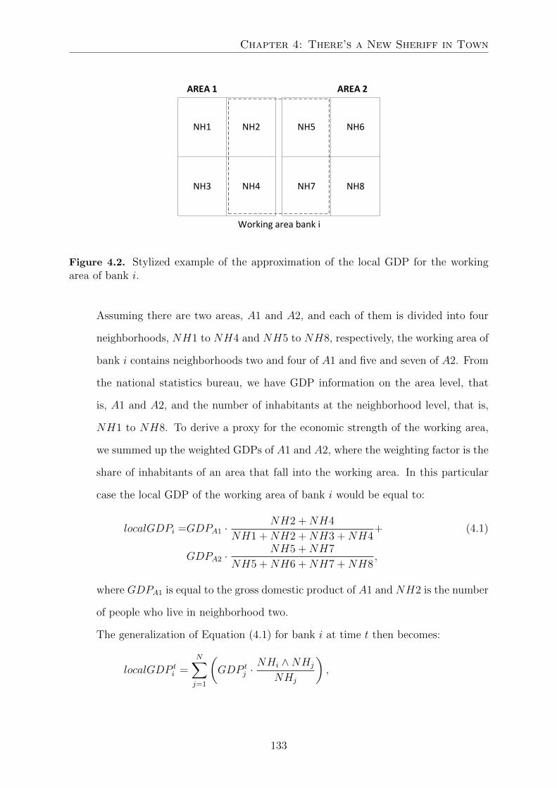
Chapter 4: There’s a New Sheriff in Town
NH4NH3
NH2NH1
NH8NH7
NH6NH5
AREA 1 AREA 2
Working area bank i
Figure 4.2. Stylized example of the approximation of the local GDP for the workingarea of bank i.
Assuming there are two areas, A1 and A2, and each of them is divided into four
neighborhoods, NH1 to NH4 and NH5 to NH8, respectively, the working area of
bank i contains neighborhoods two and four of A1 and five and seven of A2. From
the national statistics bureau, we have GDP information on the area level, that
is, A1 and A2, and the number of inhabitants at the neighborhood level, that is,
NH1 to NH8. To derive a proxy for the economic strength of the working area,
we summed up the weighted GDPs of A1 and A2, where the weighting factor is the
share of inhabitants of an area that fall into the working area. In this particular
case the local GDP of the working area of bank i would be equal to:
localGDPi =GDPA1 ·NH2 +NH4
NH1 +NH2 +NH3 +NH4+ (4.1)
GDPA2 ·NH5 +NH7
NH5 +NH6 +NH7 +NH8,
where GDPA1 is equal to the gross domestic product of A1 and NH2 is the number
of people who live in neighborhood two.
The generalization of Equation (4.1) for bank i at time t then becomes:
localGDP ti =
N∑j=1
(GDP t
j ·NHi ∧NHj
NHj
),
133

Drivers of Bank Performance and The International Cost of Equity
where N is the number of different areas (A1 and A2 in the stylized example) in the
working area of bank i. GDP tj is the GDP of area j at time t. NHj is the number
of inhabitants in area j, and NHi is the number of inhabitants in the working
area of bank i. Hence, NHi ∧ NHj is the number of inhabitants living in the
neighborhoods of area j who are also situated in the working area of bank i. Since
the assignment of neighborhoods to areas changes throughout the years, we base
the weights on population data from 2014. To obtain the number of inhabitants
in the working area of a bank, we used the number of inhabitants on the area level
and applied the same methodology as for computing the local GDP to determine
which fraction of the inhabitants in an area should be ascribed to a bank. Finally,
we divided both numbers to arrive at the local GDP per inhabitant.
CEO Turnover
CEO turnover: To measure the impact of a newly appointed CEO on the bank’s fi-
nancial performance, we add a dummy variable that equals 1 in the first year of
the new CEO. In an alternative specification, we also allow for a lagged effect by
adding a dummy variable equal to 1 in the second year of the new CEO, as well. In
predicting the impact of a change of CEO on bank performance, we focus on the
four main components of net earnings (i.e., the numerator of return on assets): net
interest income, commissions, operating expenses, and provisions for credit risks.
Insofar as a difference in ability between a predecessor and a successor arises, it
might influence the first three elements. In other words, when a high-performing
CEO is replaced by an average or low performer and the successor is able to influ-
ence performance, we expect a negative impact in terms of a decrease in net interest
income and commissions and/or an increase in costs. The opposite would occur
when a low performer is replaced by an average or high performer. In addition
to this first line of reasoning, another theory is that new CEOs might need time
to get used to their new situation, which could hamper performance in the initial
year(s) after a change. When the quality of the predecessor is not systematically
134

Chapter 4: There’s a New Sheriff in Town
different from the quality of the successor, the first situation would, on average,
have no effect on performance, while the second would have a negative impact.
It is also important to note that the final component of net earnings, provisions for
credit risks, should be distinguished from the other criteria because it is largely un-
related to the CEO’s managerial competence. Following Bornemann et al. (2015),
we differentiate between two reasons for taking provisions. First, the action might
be the result of a difference in opinion between the old and new CEOs regarding
the overall riskiness of loans. Second, the new CEO might be using the first year to
take an earnings bath and blame the old CEO for the resulting bad performance.
This opportunistic behavior is labeled taking a “big bath” (see Moore, 1973; Pour-
ciau, 1993). In the first situation, the impact on provisions and thus performance is
unclear, while the second avenue would increase provisions and lower performance.
Although it is unsure which of these channels will dominate, taken together, they
predict a negative impact on results. We therefore expect a decline in financial
performance after a change in CEO.
4.4 Data
We relied on three main sources of data for this chapter: the financial cooperative under
study, the national statistics bureau, and LinkedIn. In this section, we discuss the data
and provide summary statistics.
4.4.1 Bank Data
The financial cooperative provided annual data on its balance sheet, income statement,
number of members, working areas, and market shares in two different sectors (resi-
135

Drivers of Bank Performance and The International Cost of Equity
dential mortgages and food and agriculture) per bank for the 2010–2015 period.7,8 In
addition, we were provided with the names of the CEOs of the local banks during that
sample period. In contrast to the financial data, this latter dataset was incomplete and
required additional work (see Section 4.4.3).
During the period we considered, 41 banks merged. Typically, one bank was the
leading bank and the other the liquidated bank. Figure 4.3 provides an example.
Bank A
0 1 2 3
Bank B
Bank C
Figure 4.3. Banks A and B merge at Time 1. Bank B is the leading bank and Bank Ais the liquidated bank. Bank C is equal to the merged entity as of Time 1. Before themerger (from period 0 to 1), Bank C is equal to the combination of the individual BanksA and B.
Suppose a merger takes place at Time 1 between the liquidated Bank A and the
leading Bank B. That means that after time period 1, Bank A no longer exists and is in-
corporated into Bank B. To ensure comparability before and after the merger, we define
a hypothetical Bank C, which is the equivalent of Bank B from Period 1 to Period 3.
In the pre-merger period, i.e., from Periods 0 to 1, we artificially “merge” Bank A with
Bank B to form Bank C. Hence, for this period, we combine the financial data of Banks
A and B. In the sample, we then only include Bank C and do not consider Banks A and B.
For the assignment of a CEO to a bank, we apply the rule that the CEO of the
leading bank becomes the CEO of the “combined” bank. Hence, in the above example,
7Note that the market share data provided for the two sectors is not measured the same way. Themarket share in mortgages is based on bank data and data from the cadastre. The market share iscomputed as the euro amount of mortgages on the bank’s balance sheet divided by the total euroamount of mortgages in the working area of the bank. The market share for the food and agriculturesector is based on an annual survey of the companies in the working area of the bank. It is defined asthe number of surveyed companies in that sector that perceive the bank as their house bank divided bythe total number of surveyed companies in the food and agriculture sector.
8This data is not publicly available and was provided by the bank.
136

Chapter 4: There’s a New Sheriff in Town
the CEO who led Bank B from Periods 0 to 3 becomes the CEO of Bank C in Periods
0 to 3. This resulted in 106 banks for the period from 2010 to 2015. We also requested
financial data for the period before 2010, but this data was either not consistent with
the data after 2010 or unavailable.
4.4.2 National Statistics Bureau Data
As a proxy for the economic activity of a local bank’s working area, we gathered data
from the national statistics bureau on GDP levels and number of inhabitants. In 1970,
the country under study was divided into 40 areas by applying a nodal classification
system which was based on commuter flows. That is, each area has a central node (a
city) and a surrounding area depending on it. On this level, we have data for GDP
levels and the number of inhabitants from 2010 to 2015. Independent of this structure,
the country is divided into multiple provinces, each consisting of several municipalities.
Each municipality is in turn further divided into quarters and neighborhoods. On the
neighborhood level, we obtained data for the number of inhabitants in 2014.
4.4.3 CEO Data
The previous two data sources cover bank-, industry-, and region-specific variables. Yet,
in order to assess the impact of the CEOs on bank performance, we also need information
on their exit and start dates. The financial cooperative provided us with this information,
which we enriched with information from the CEOs’ LinkedIn profiles. If the information
between these two sources did not correspond, we relied on the dates provided by the
CEOs on their LinkedIn profiles, because we considered that to be more trustworthy.
This combined dataset was then used to assign the CEOs to bank-years according to the
following assignment rules:
1. The CEO in charge for the majority of the year, with a minimum of six months,
is assigned as CEO. Hence, if the predecessor left on 31-5-2011 and the successor
started on 1-6-2011, the latter was assigned to the bank for 2011;9
9This assignment rule might introduce a bias when there are CEOs who were at the helm for less
137
Drivers of Bank Performance and The International Cost of Equity
2. If both the predecessor and the successor were CEO for six months each – that
is, the predecessor left on 30-6-2011 and the successor started on 1-7-2011 – we
assigned the bank to the successor;
3. If a CEO started at a bank as an ad interim CEO and subsequently became the
permanent successor, the bank was assigned to the new CEO as of the start of the
ad interim period;10
4. Bank-years not assigned to a particular CEO after applying the above rules were
assigned to the predecessor.
As indicated by Rule 4, a few bank-years remained after applying Rules 1 through 3
above for which no CEO had been assigned. For instance, if the predecessor left on 1-8-
2011 and the successor started on 1-8-2013, the bank was assigned to the successor for
2014 and to the predecessor through 2011, but it lacked an assignation for the interven-
ing years, 2012 and 2013. Since our main analyses focus on the impact of the successors,
it is important that their moment of arrival not be modified. Of less importance is when
the predecessor left. These empty years were therefore assigned to the predecessor. In
sum, this procedure ensures that a bank-year is only assigned to the successor once they
have been CEO for at least six months. We will subsequently refer to this data file as
the successor file.
In addition to analyses focusing on the impact of the successor, we are interested in
the relationship between the departure of a CEO and bank performance. For instance,
we wonder whether CEOs who are being promoted were strong performers in their final
year before departure. In that case, our focus shifts from the successor to the predecessor
and, as a result, assignment rules number 2 and 4 change. When both predecessor and
than six months. These CEOs would then not be assigned to a bank-year because of the six monthsrule. Fortunately, this did not occur in our dataset.
10If these cases frequently occurred in our dataset and would drive the overall result, the followinginterpretation might apply: an ad interim CEO takes an earnings bath to blame the previous board,which decreases the likelihood of other board members to become the new CEO and at the same timeincreases the ad interim CEO’s chances to become the permanent CEO. Only in four of the 80 CEOchanges an ad interim CEO became the permanent CEO. Hence, these cases are unlikely to drive ouroverall results.
138

Chapter 4: There’s a New Sheriff in Town
successor are CEO for six months each, the bank-year is assigned to the predecessor.
Furthermore, the empty years are now assigned to the successor, because the more
important criterion is when the predecessor left, rather than when the successor started.
Consequently, these rules ensure that a bank-year is only assigned to the predecessor
when they have been CEO for at least six months. We will subsequently refer to this
data file as the predecessor file.
4.5 Summary Statistics
In this section, we first present summary statistics for the bank characteristics; then we
present those for the CEO turnover variables.
4.5.1 Bank Characteristics
Table 4.1 contains summary statistics for the characteristics of the banks.
Table 4.1. Summary statistics of bank characteristics. The statistics are computed overtime and across banks. Assets are measured in thousands of euros and Local GDP perinhabitant in euros. The other variables are expressed as percentages.
Mean SD Min Max
RoA (%) 0.37 0.34 -1.28 1.54Assets (’000 ¤) 2,720,498 1,344,617 235,322 10,935,552Retail Loans to Assets (%) 59.27 8.15 31.19 79.67Mortgages to Retail Loans (%) 99.41 0.33 93.61 99.76Equity to Assets (%) 8.61 2.53 0.37 16.61Deposits to Assets (%) 71.92 9.67 35.10 90.26Debt to Central Institution to Assets (%) 17.35 10.70 0.00 62.38Impaired Loans to Total Loans (%) 1.42 0.65 0.14 4.30Member Ratio (%) 26.01 7.49 9.12 57.39Market Share in Mortgages (%) 24.59 7.97 8.69 51.84Market Share in Food/Agri (%) 82.77 7.18 55.56 96.08Local GDP per Inhabitant (¤) 36,157 8,953 17,549 71,121
Number of observations 530
The statistics were computed over time and across banks. The average return on
assets of a local bank equals 0.37%, with a minimum of -1.28% and a maximum of
139

Drivers of Bank Performance and The International Cost of Equity
1.54%. The average size of a bank, measured by assets, equals ¤2.7 billion. The third
row shows that retail loans, which are almost entirely composed of mortgages (fourth
row), account for 59% of total assets. On the liability side, equity accounts for 8.6%
of the balance sheet. The minimum and maximum values of 0.37% and 16.61% show,
respectively, that some member banks are almost depleted of capital, while others have
plenty. Deposits (retail and company) account for 72% of the funding and debt to the
central institution for 17%. Considering the minimum and maximum values of this latter
variable, some banks need no funding from the central institution at all, while others
require up to 62%. The percentage of impaired to total loans ranges from 0.14% to
4.30%, with an average of 1.42%. The market share of 83% on average in food and
agriculture is remarkable. Finally, local GDP per inhabitant highlights the variation in
economic activity between the working areas.
4.5.2 CEO Turnover Variables
Since our main analyses focus on the impact of a successor on bank performance, we
discuss here the characteristics of that data file.11 Seventy of the 106 banks experienced
a CEO changeover once between 2010 and 2015, and for five banks, the CEO changed
twice. We classify the causes for these 80 departures into three categories: positive,
neutral, and negative. The first category consists of cases where a CEO was promoted
and the third of cases where they were dismissed or demoted. In the neutral category,
the departure of the CEO was unrelated to performance or involved switching to another
bank of similar size. An overview of the number of departures and the associated reason
is provided in Table 4.2.
11See Section 4.4.3 for a discussion of the differences between the data files focusing on predecessorsand successors.
140
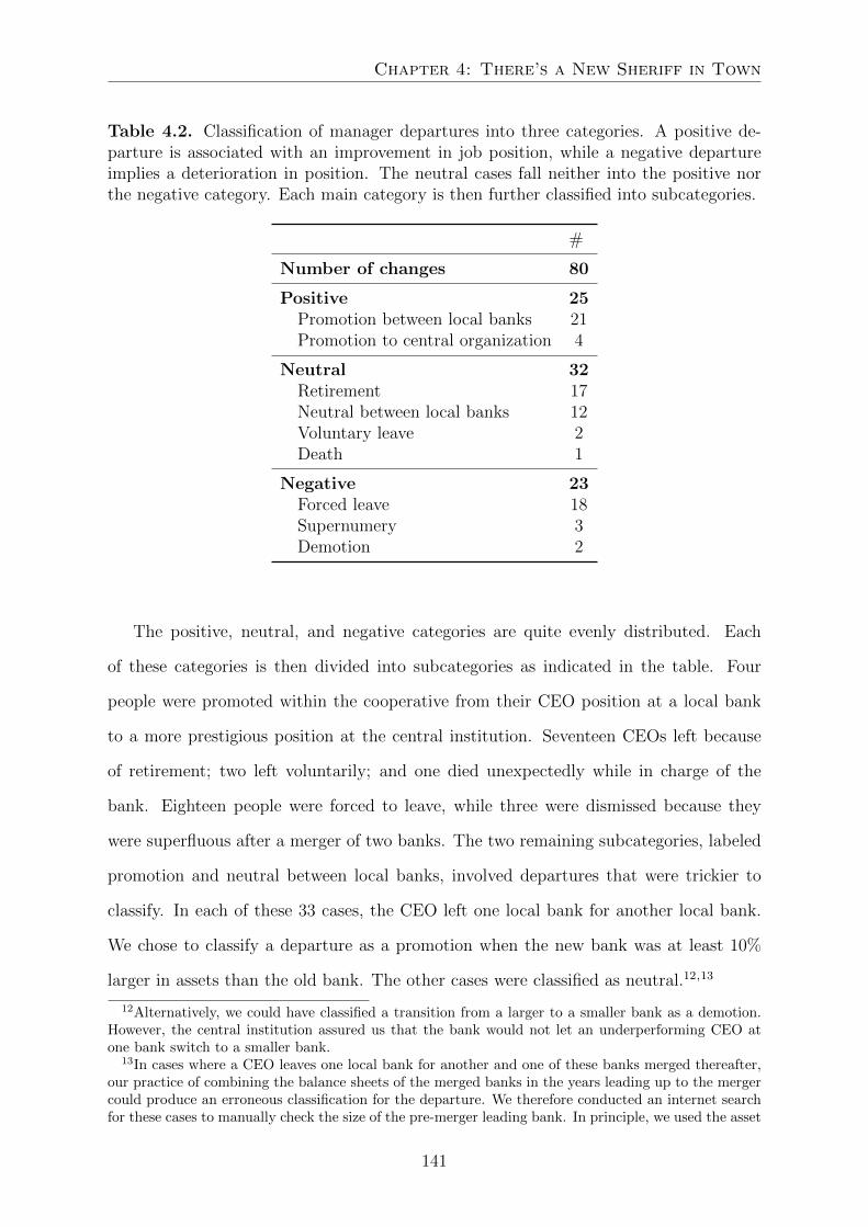
Chapter 4: There’s a New Sheriff in Town
Table 4.2. Classification of manager departures into three categories. A positive de-parture is associated with an improvement in job position, while a negative departureimplies a deterioration in position. The neutral cases fall neither into the positive northe negative category. Each main category is then further classified into subcategories.
#
Number of changes 80
Positive 25Promotion between local banks 21Promotion to central organization 4
Neutral 32Retirement 17Neutral between local banks 12Voluntary leave 2Death 1
Negative 23Forced leave 18Supernumery 3Demotion 2
The positive, neutral, and negative categories are quite evenly distributed. Each
of these categories is then divided into subcategories as indicated in the table. Four
people were promoted within the cooperative from their CEO position at a local bank
to a more prestigious position at the central institution. Seventeen CEOs left because
of retirement; two left voluntarily; and one died unexpectedly while in charge of the
bank. Eighteen people were forced to leave, while three were dismissed because they
were superfluous after a merger of two banks. The two remaining subcategories, labeled
promotion and neutral between local banks, involved departures that were trickier to
classify. In each of these 33 cases, the CEO left one local bank for another local bank.
We chose to classify a departure as a promotion when the new bank was at least 10%
larger in assets than the old bank. The other cases were classified as neutral.12,13
12Alternatively, we could have classified a transition from a larger to a smaller bank as a demotion.However, the central institution assured us that the bank would not let an underperforming CEO atone bank switch to a smaller bank.
13In cases where a CEO leaves one local bank for another and one of these banks merged thereafter,our practice of combining the balance sheets of the merged banks in the years leading up to the mergercould produce an erroneous classification for the departure. We therefore conducted an internet searchfor these cases to manually check the size of the pre-merger leading bank. In principle, we used the asset
141

Drivers of Bank Performance and The International Cost of Equity
4.6 Results
In this section, we present our results. In Section 4.6.1, we relate financial bank perfor-
mance to bank characteristics. In Sections 4.6.2 to 4.6.4, we assess the impact of CEO
turnover on bank performance.
4.6.1 Bank Characteristics
We estimate the following fixed effects model:
RoAit = α + κt + σi + βXit + εit, (4.2)
where RoAit is the return on assets for bank i at time t ∈ {2011, 2012, 2013, 2014, 2015}
Time and bank fixed effects are indicated by κt and σi, respectively, and α is the constant.
Xit represents the control variables for bank i at time t. We estimate the model with
the fixed effects specification because we do not expect the strict exogeneity assumption
to be violated (Cameron & Trivedi, 2009, pg. 271).14,15 In the fixed effects model,
we include bank characteristics that are assumed not to change over time, such as the
bank’s culture, and time effects that do not differ between banks, such as, a nationwide
economic downturn. Moreover, to correct for arbitrary heteroskedasticity and arbitrary
correlation over time within the local bank (i.e., within-group correlation), the error
terms are clustered at the bank level. Finally, to limit the impact of outliers on the
results, we apply a logarithmic transformation to the size (assets) and local GDP per
inhabitant variables.
size in the year prior to the merger. If this was not available, we used the last year before the mergerfor which there was data available. When we were not able to identify the size of the pre-merger leadingbank, we estimated it by applying the same division in assets between the leading and liquidated bankas we observed in the cases where we were able to identify the size of the pre-merger leading bank.
14We also estimated a first-difference specification of the model. This changed the results in twoways: the size of the bank became significantly negatively related to performance at the 5% levelinstead of at the 10% level. Moreover, local GDP per inhabitant was now significantly positively relatedto performance at the 5% level.
15We tested for the appropriateness of the random effects model by using a robust version (i.e.,cluster-robust standard errors) of the Hausman test (Cameron & Trivedi, 2009, pp. 266–268). The nullof equality of coefficients between the fixed and random effects model was rejected (p-value of 0.0000).Hence, the random effects model is not appropriate in this setting.
142

Chapter 4: There’s a New Sheriff in Town
Table 4.3. Results of a fixed effects model with return on assets as dependent variable.Balance sheet characteristics, local GDP per inhabitant, market shares, and memberratio are the independent variables. Time and bank fixed effects are included, and theerror terms are clustered per bank. The p-values are reported in parentheses under theparameter estimates.
(1) (2)
Log(Assets) -0.829∗ -0.825∗
(0.083) (0.085)
Retail loans to assets 0.0122 0.0123(0.153) (0.148)
Equity to assets -0.157∗∗∗ -0.150∗∗∗
(0.000) (0.001)
Impaired loans 0.0214 0.0281to total loans (0.708) (0.622)
Debt to central -0.00760institution to assets (0.316)
Log (Local GDP 0.804 0.809per inhabitant) (0.227) (0.226)
Market share 0.00568 0.00565in mortgages (0.200) (0.202)
Market share 0.00208 0.00208in food/agri (0.743) (0.744)
Member ratio -0.00620 -0.00621(0.396) (0.397)
Deposits to assets 0.00759(0.312)
Observations 530 530Bank fixed effects Yes YesTime fixed effects Yes YesClustering level Bank Bank
p-values in parentheses∗ p < 0.10, ∗∗ p < 0.05, ∗∗∗ p < 0.01
We estimated two specifications of the fixed effects model presented in Equation
(4.2). In the first specification, we included debt to the central institution to assets as an
independent variable, while this variable is replaced by deposits to assets in the second
specification. We could not include both variables in one specification because it would
have led to multicollinearity, since the sum of these two variables and equity to assets is
approximately equal to 1.
143

Drivers of Bank Performance and The International Cost of Equity
The results are similar for Specifications 1 and 2. Size, as measured by log(assets),
and equity to assets are negatively related to return on assets at the 10% and 1% levels,
respectively. Positive economies of scale (Altunbas & Molyneux, 1996; McAllister & Mc-
Manus, 1993) and the ability to diversify (McAllister & McManus, 1993), which predict
a positive association between size and performance, do not apply in our case. On the
contrary, our results suggest diseconomies of scale, which might be attributable to the
increased complexity of a larger bank. In addition, large banks are primarily located
in large cities, where competition is fiercer16 than in rural areas and the impact of the
economic recession(s) might have been more severe.
Berger (1995b) points to a lower tax shield for banks with a great deal of equity as
an explanation for the negative association between equity to assets and profitability.
Alternatively, rapid expansion on the part of a bank in preceding years would lengthen
its balance sheet and could lead to a decrease in the equity to assets ratio in cases where
retained earnings are insufficient for keeping up with the expansion. In an unreported
regression, we tested this hypothesis by adding asset growth in the previous year as an
independent variable. In that specification, the association between equity to assets and
profitability remained unchanged.
Although insignificant, the existence of a larger fraction of retail loans (which in our
case consist almost exclusively of mortgages) is positively related to performance. The
low default rate and steady income associated with mortgages seems to predominate over
the higher interest rates associated with company loans. This is in line with the finding
of Delis and Kouretas (2011), who documented that the low-interest-rate environment
of the 2000s led to an increase in risk-taking at banks. Insofar as this resulted in an
increase in company loans vis-a-vis mortgages, the banks that increased their riskiness
16Although we already proxy for competition with the market share variables for mortgages andfood/agriculture, we do not have similar data for the most profitable market for local banks: companyloans. Therefore, competition on this dimension (i.e., larger banks face more competition) could bepartly captured by the size of the bank.
144

Chapter 4: There’s a New Sheriff in Town
the most are the most likely to have experienced the deterioration of these company
loans in the economic crisis, which unfolded during the years of our sample. Ultimately,
this then also harmed their profitability.
The positive relationship between performance and local GDP per inhabitant is in
line with the results of Barth et al. (2003) and Demirguc-Kunt and Huizinga (1999).
Moreover, when we estimate a first-difference specification of the model, that relationship
becomes statistically significant at the 5% level. Finally, the member ratio, which we
use as a proxy for customer loyalty, has an insignificant negative sign, while we expected
it to have a positive impact on bank performance. A discussion contrasting the possible
interpretations of this finding – that is, whether loyalty is not a determining factor in
bank profitability or the member ratio is not a proper proxy for loyalty – is outside the
scope of this chapter.
4.6.2 Impact of CEO Turnover on Performance
In this section, we use the statistically significant financial characteristics of the previous
section and add dummies to measure the impact of CEO turnover on a bank’s financial
performance. We used the successor data file (see Section 4.4.3) for these analyses. We
estimate the following fixed effects model:
RoAit = α + κt + σi + βXit + λτEτ + εit, (4.3)
where we have added the dummy Eτ with τ ∈ {−1, 0, 1, 2, 3, 4, 5}, to Equation (4.2).
Depending on the regression specification, we include a subset of these dummies. The
dummy E1 is equal to 1 in the first year of the new CEO and E2 is equal to 1 in the
second year of the new CEO. The last year of the previous CEO is indicated by E0. To
enhance readability, we omit subindices i and t for the dummy variables. To clarify how
the dummies should be interpreted, we present a stylized example for a CEO changeover
at Bank A in Table 4.4.
145
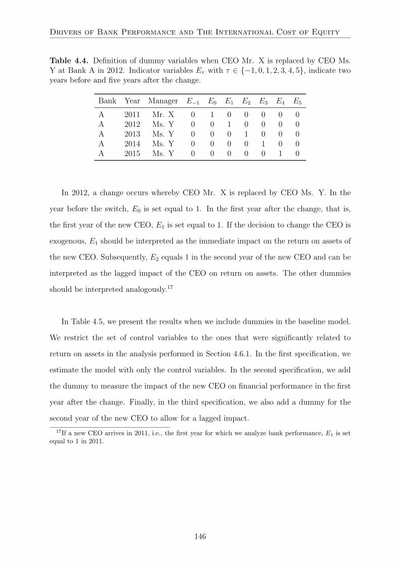
Drivers of Bank Performance and The International Cost of Equity
Table 4.4. Definition of dummy variables when CEO Mr. X is replaced by CEO Ms.Y at Bank A in 2012. Indicator variables Eτ with τ ∈ {−1, 0, 1, 2, 3, 4, 5}, indicate twoyears before and five years after the change.
Bank Year Manager E−1 E0 E1 E2 E3 E4 E5
A 2011 Mr. X 0 1 0 0 0 0 0A 2012 Ms. Y 0 0 1 0 0 0 0A 2013 Ms. Y 0 0 0 1 0 0 0A 2014 Ms. Y 0 0 0 0 1 0 0A 2015 Ms. Y 0 0 0 0 0 1 0
In 2012, a change occurs whereby CEO Mr. X is replaced by CEO Ms. Y. In the
year before the switch, E0 is set equal to 1. In the first year after the change, that is,
the first year of the new CEO, E1 is set equal to 1. If the decision to change the CEO is
exogenous, E1 should be interpreted as the immediate impact on the return on assets of
the new CEO. Subsequently, E2 equals 1 in the second year of the new CEO and can be
interpreted as the lagged impact of the CEO on return on assets. The other dummies
should be interpreted analogously.17
In Table 4.5, we present the results when we include dummies in the baseline model.
We restrict the set of control variables to the ones that were significantly related to
return on assets in the analysis performed in Section 4.6.1. In the first specification, we
estimate the model with only the control variables. In the second specification, we add
the dummy to measure the impact of the new CEO on financial performance in the first
year after the change. Finally, in the third specification, we also add a dummy for the
second year of the new CEO to allow for a lagged impact.
17If a new CEO arrives in 2011, i.e., the first year for which we analyze bank performance, E1 is setequal to 1 in 2011.
146

Chapter 4: There’s a New Sheriff in Town
Table 4.5. Results for a fixed effects model with return on assets as dependent variable.We only include control variables that were significantly related to return on assets inSection 4.6.1. We include dummies for the first year of the new CEO, E1, in Specification(2) and for the first and second years, E1 and E2, in Specification (3). Time and bankfixed effects are included, and the error terms are clustered per bank. The p-values arereported in parentheses under the parameter estimates.
(1) (2) (3)
Log(Assets) -1.109∗∗ -1.140∗∗ -1.156∗∗∗
(0.012) (0.010) (0.009)
Equity to assets -0.155∗∗∗ -0.156∗∗∗ -0.154∗∗∗
(0.000) (0.000) (0.000)
E1 -0.0765∗ -0.0950∗∗
(0.058) (0.019)
E2 -0.0768∗∗
(0.048)
Observations 530 530 530
p-values in parentheses∗ p < 0.10, ∗∗ p < 0.05, ∗∗∗ p < 0.01
The results for the control variables are the same in all three specifications. Com-
pared to the results of Section 4.6.1, the significance of size increases from the 10% to
the 1% level. The second specification shows that in the first year of a new CEO, the
return on assets drops significantly, with a p-value of the 5.8%. In economic terms, the
impact is quite significant, since a change in CEO reduces the return on average assets
by -0.08 percentage points in the first year, which equals 23% of the standard deviation
of return on assets (see Table 4.1). When we also allow for a lagged effect in the change
of CEO, Specification 3, we observe a significant decline in performance in both the first
and second years after the change. Adding both effects amounts to a decrease in return
on assets of 0.17 percentage points over the first two years.18
18Rajan (1994) documented that banks are more likely to increase their provisions when other banksin the same region increase their provisions. In order to check whether this phenomenon of “taking anearnings bath together” might also apply to our case, we rerun Specification 2 and 3 of Table 4.5 whileclustering the standard errors on the regional instead of on the bank level. The regions have between 6and 12 local banks. Naturally, the regression coefficients are the same. Moreover, the significance of thevariables are also largely similar: including only the first year dummy (see Specification 2) increases thesignificance from the 10% to the 5% level, and including the first two years (see Specification 3) slightly
147

Drivers of Bank Performance and The International Cost of Equity
Before going on to analyze the various factors that could explain the decrease in
performance (see Sections 4.6.3 and 4.6.4), we would like to first discuss a possible en-
dogeneity issue. If we consider that bank performance might influence decisions about
replacing a CEO, our setup could be considered vulnerable to the issue of reverse causal-
ity. For example, the CEO of a bank that is performing well, whether or not due to that
CEO’s influence, might be rewarded in the form of a promotion. In that case, strong
prior bank performance has induced the CEO change. The exact opposite can happen
when a CEO at a poorly performing bank is dismissed or demoted within the organiza-
tion. As a stylized example, consider the case of strong performance on the part of bank
i in year t, which leads to a high εi,t. If we assume that this implies that the CEO will be
rewarded and therefore leave the bank in year t, this yields a positive correlation between
εi,t and E1,i,t, that is, the first year of the new CEO. This would violate the exogeneity
assumption and that renders a causal interpretation of the results problematic.
However, the method we used for assigning a CEO to a bank partially mitigates this
problem, since the CEO who is at the helm for the longest portion of the year is classified
as the CEO for that year. The problem described above therefore only occurs when a
CEO is promoted in the first half of the year and the new CEO has no influence on the
bank’s performance until the end of the calendar year. In that case, the bank’s perfor-
mance in year t is determined by the leaving CEO and is correlated with the dummy
variable equal to 1 in year t, that is, the first year of the new CEO. While such a case is
rather unlikely, it could occur in our sample. We therefore resorted to an instrumental
variable fixed effects (IV-FE) analysis.19
We look for exogenous variation that is correlated with the dummy variable E1,i,t,
increases the significance of the first year and decreases the significance of the second year from the 5%to the 10% level. In sum, the results are robust to this alternative specification.
19Another motivation to perform an IV-FE analysis is the “romance of leadership” theory presentedin Meindl, Ehrlich, and Dukerich (1985). The authors are worried about assigning too much powerto leaders of organizations in influencing its outcomes. This concern of omitted variables, which canpotentially account for the relationship we find, is mitigated with the IV-FE analysis.
148
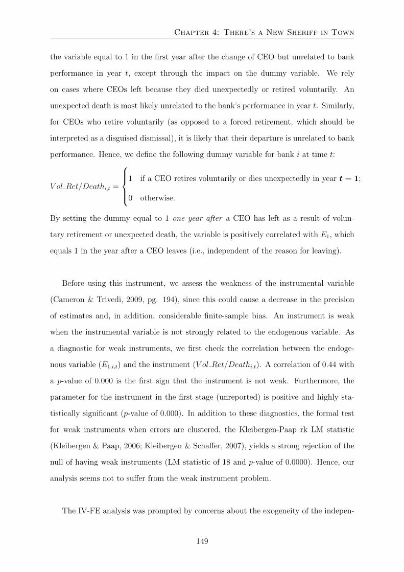
Chapter 4: There’s a New Sheriff in Town
the variable equal to 1 in the first year after the change of CEO but unrelated to bank
performance in year t, except through the impact on the dummy variable. We rely
on cases where CEOs left because they died unexpectedly or retired voluntarily. An
unexpected death is most likely unrelated to the bank’s performance in year t. Similarly,
for CEOs who retire voluntarily (as opposed to a forced retirement, which should be
interpreted as a disguised dismissal), it is likely that their departure is unrelated to bank
performance. Hence, we define the following dummy variable for bank i at time t:
V ol Ret/Deathi,t =
1 if a CEO retires voluntarily or dies unexpectedly in year t − 1;
0 otherwise.
By setting the dummy equal to 1 one year after a CEO has left as a result of volun-
tary retirement or unexpected death, the variable is positively correlated with E1, which
equals 1 in the year after a CEO leaves (i.e., independent of the reason for leaving).
Before using this instrument, we assess the weakness of the instrumental variable
(Cameron & Trivedi, 2009, pg. 194), since this could cause a decrease in the precision
of estimates and, in addition, considerable finite-sample bias. An instrument is weak
when the instrumental variable is not strongly related to the endogenous variable. As
a diagnostic for weak instruments, we first check the correlation between the endoge-
nous variable (E1,i,t) and the instrument (V ol Ret/Deathi,t). A correlation of 0.44 with
a p-value of 0.000 is the first sign that the instrument is not weak. Furthermore, the
parameter for the instrument in the first stage (unreported) is positive and highly sta-
tistically significant (p-value of 0.000). In addition to these diagnostics, the formal test
for weak instruments when errors are clustered, the Kleibergen-Paap rk LM statistic
(Kleibergen & Paap, 2006; Kleibergen & Schaffer, 2007), yields a strong rejection of the
null of having weak instruments (LM statistic of 18 and p-value of 0.0000). Hence, our
analysis seems not to suffer from the weak instrument problem.
The IV-FE analysis was prompted by concerns about the exogeneity of the indepen-
149

Drivers of Bank Performance and The International Cost of Equity
dent variable of interest. If this variable were exogenous, the IV-FE technique would be
much less efficient than regular fixed effects estimation (Cameron & Trivedi, 2009, pg.
188), which weakens the significance of the results. We must therefore first test whether
E1 is exogenous. To do this, we compare the parameter estimates of the regular fixed
effects estimation with those of an IV-FE estimation. In our case, the estimate for the
impact of a new CEO in the first year equals -0.0765 using regular fixed effects (see Table
4.5) and -0.2073 (unreported) with IV-FE. We formally test whether there is a difference
in these parameter estimates by applying the C statistic, which is a generalization of the
Durbin-Wu-Hausman test in the sense that it allows for heteroskedasticity (Cameron &
Trivedi, 2009, pp. 188–190; Hayashi, 2000, pp. 233–234). In our case, we are not able
to reject the null that the coefficients are equal (p-value of 0.2049); hence, we cannot
reject the null that the regressor is exogenous.20 This result, combined with our earlier
observation that cases resulting in reverse causality are unlikely to occur, significantly
reduces our concerns about the problem of endogeneity.
4.6.3 Reason for CEO Turnover
Several possible explanations for the decrease in performance in the first two years after
a change in CEO can be identified. It might be caused by a deterioration of net interest
income or commissions or a spike in operating expenses. This, in turn, could be the
result of a couple of factors: the new CEO might need time to get used to the bank, its
people, and the local community, or they might simply be a worse executive than the old
CEO. Bank performance could also drop as a result of an increase in the provisions for
credit risks. Increasing provisions can be motivated by a difference in opinion between
the new and the old CEOs regarding credit risk. Such increase can also be influenced
by other factors, though, such as a need to offset a decrease in provisions taken in the
final year of an exiting CEO, as part of a strategy to show increased performance prior
to departure, or when a new CEO wants to take a so-called earnings bath (Bornemann
20We repeated these analyses where we also included the lagged effect, E2 (Specification 3 of Table4.5). The results were similar. The Kleibergen-Paap rk LM statistic rejects the null of weak instruments,with a p-value of 0.0000, while the p-value of the C statistic equals 0.2148.
150

Chapter 4: There’s a New Sheriff in Town
et al., 2015). Bornemann et al. (2015) provide empirical evidence of this “big bath”
theory for CEO changes at German savings banks. The initial poor performance at the
bank is then implicitly ascribed to the previous CEO, and when performance rebounds
in subsequent years, this is ascribed to the new CEO.
It is not possible to determine from the results presented in Table 4.5 above which of
these explanations is the most likely determinant of performance variation. We therefore
analyze each one separately to identify the most likely cause of decreased performance
after CEO turnover. We first consider whether it is related to new CEOs being of lower
quality than the departing CEOs by zooming in on the various reasons of departure.21
Table 4.2 above contains an overview of the three main categories of departure: positive,
neutral, and negative. The positive category is composed of CEOs that have been pro-
moted, while the negative category contains dismissed or demoted CEOs. A departure is
designated as neutral when a CEO leaves for reasons unrelated to performance or trans-
fers to another local bank that is not significantly larger. In order to assess whether we
find heterogeneous effects on performance for different reasons of departure, we estimate
the following fixed effects regression model:
RoAit = α + κt + σi + βXit +∑
τ={1,2}
∑k∈{+,=,−}
λτ,kEτRDki,t + εit, (4.4)
where RDki,t is a dummy equal to 1 when a CEO leaves bank i with reason k in year
t − 1. The reason for departure, k, can take on three values: positive (+), neutral (=),
or negative (-). Hence, the three dummies, RDki,t, allow us to evaluate the performance
of the new CEO distinguishing between each reason for the predecessor’s departure. In
Table 4.6 we present the results for when only the first year of the new CEO is included,
that is τ equals 1 (Specification 1) and when the new CEO’s second year is added as
well, that is τ equals 1 and 2 (Specification 2).
21In this setting, quality should be interpreted as attributes that are relevant for leading a local bank,cf. Jenter et al. (2016). This is the same as the use of “talent” in Gabaix and Landier (2008) and“managerial ability” in Tervio (2008).
151
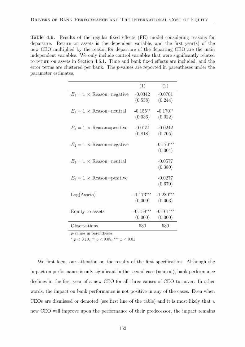
Drivers of Bank Performance and The International Cost of Equity
Table 4.6. Results of the regular fixed effects (FE) model considering reasons fordeparture. Return on assets is the dependent variable, and the first year(s) of thenew CEO multiplied by the reason for departure of the departing CEO are the mainindependent variables. We only include control variables that were significantly relatedto return on assets in Section 4.6.1. Time and bank fixed effects are included, and theerror terms are clustered per bank. The p-values are reported in parentheses under theparameter estimates.
(1) (2)
E1 = 1 × Reason=negative -0.0342 -0.0701(0.538) (0.244)
E1 = 1 × Reason=neutral -0.155∗∗ -0.170∗∗
(0.036) (0.022)
E1 = 1 × Reason=positive -0.0151 -0.0242(0.818) (0.705)
E2 = 1 × Reason=negative -0.170∗∗∗
(0.004)
E2 = 1 × Reason=neutral -0.0577(0.380)
E2 = 1 × Reason=positive -0.0277(0.670)
Log(Assets) -1.173∗∗∗ -1.280∗∗∗
(0.009) (0.003)
Equity to assets -0.159∗∗∗ -0.161∗∗∗
(0.000) (0.000)
Observations 530 530
p-values in parentheses∗ p < 0.10, ∗∗ p < 0.05, ∗∗∗ p < 0.01
We first focus our attention on the results of the first specification. Although the
impact on performance is only significant in the second case (neutral), bank performance
declines in the first year of a new CEO for all three causes of CEO turnover. In other
words, the impact on bank performance is not positive in any of the cases. Even when
CEOs are dismissed or demoted (see first line of the table) and it is most likely that a
new CEO will improve upon the performance of their predecessor, the impact remains
152

Chapter 4: There’s a New Sheriff in Town
non-positive. We must, however, realize that CEOs could also be dismissed for reasons
unrelated to financial performance, such as disagreement within the executive board or a
lack of trust between the executive and supervisory boards. When a difference in quality
between the old and new CEOs is the presumed explanation for the overall finding of
a decline in performance, we would have expected the largest decline in performance to
be in cases where a CEO has been promoted (line three). This is not what we find: the
impact on performance in these cases is almost equal to 0. On the other hand, when
the reason for departure is neutral (line two), the decline in performance is statistically
significant at the 5% level. Differences in quality between the predecessor and successor
would explain this result only in cases where the successors were systematically worse
than the predecessors.
The results in the second specification are similar to those of the first specification for
the first year of the new CEO. Moreover, the impact on performance in the second year
is once again non-positive for all three causes of departure. However, in contrast to the
neutral category in the first year, the cases where the former CEO has been dismissed
or demoted (line four) now drive the overall negative impact on bank performance (see
Specification 3 of Table 4.5). This result would only be consistent with the difference-in-
quality explanation if the new CEOs were systematically worse than the old CEOs who
left for a negative reason. Finally, and in line with the results for the first year, the neg-
ative impact on performance is smallest in cases where the former CEO was promoted,
which is the opposite of what we would have expected if differences in CEO quality were
the driving force behind the results.
In order to assess how departing CEOs performed in their last year, and whether this
might explain the change in performance in the first year of the new CEO, we estimate
the following model:
RoAit = α + κt + σi + βXit +∑
k∈{+,=,−}λkE0RD
ki,t + εit, (4.5)
153

Drivers of Bank Performance and The International Cost of Equity
which is the same as Equation (4.4), except that we now focus on the last year of the old
CEO, E0. Since the attention is shifted to the departing CEO, we use the predecessor
file for this analysis (see Section 4.4.3).22 Results are presented in Table 4.7.
Table 4.7. Results of the regular fixed effects (FE) model considering reasons for depar-ture. Return on assets is the dependent variable and the last year of the departing CEOmultiplied by the reason for departure of the departing CEO are the main independentvariables. We only include control variables that were significantly related to return onassets in Section 4.6.1. Time and bank fixed effects are included, and the error termsare clustered per bank. The p-values are reported in parentheses under the parameterestimates.
(1)
E0 = 1 × Reason=negative -0.0320(0.611)
E0 = 1 × Reason=neutral -0.0580(0.246)
E0 = 1 × Reason=positive 0.0633(0.142)
Log(Assets) -1.105∗∗
(0.012)
Equity to assets -0.152∗∗∗
(0.000)
Observations 530
p-values in parentheses∗ p < 0.10, ∗∗ p < 0.05, ∗∗∗ p < 0.01
We do not document a statistically significant difference in performance in the final
year of a former CEO’s tenure for any of the reasons of departure. Moreover, when we
test whether the coefficients pertaining to the three reasons of departure are jointly equal
to 0, we cannot reject this null (p-value of 0.2602). We discuss the implications of these
results separately for each of the three categories below.
22In 10 instances, 2015 was the last year of a departing CEO. Since 2015 was the last year of our data,these cases are irrelevant for the analyses related to the first year(s) of a new CEO. For the analysesrelated to the last year of an exiting CEO, however, they have been included.
154
Chapter 4: There’s a New Sheriff in Town
It appears that CEOs who were dismissed or demoted (first line) were not significantly
underperforming. As suggested above, other considerations than financial performance
might have played a role in these cases. Moreover, they were also not outperforming,
which makes it unlikely that the outperformance in the second year of a new CEO (see
Specification 2 of Table 4.6) can be explained by a difference in quality. CEOs who
left due to a neutral reason (second line) neither underperform nor outperform in their
final year. This renders it unlikely that a difference in quality between predecessor and
successor explains the results for the neutral category in the first year of Table 4.6,
because in that case we would have expected a significant outperformance (and not a
slight underperformance) in the final year of the predecessor (see Table 4.7). Finally,
although insignificant, CEOs who were promoted show the strongest performance in the
year before departure. The difference-in-quality explanation would then prescribe the
strongest decline in performance in the first years of the new CEO for such cases, which is
the exact opposite of what we have documented in Table 4.6. This thus undermines the
difference-in-quality explanation even further. We must therefore turn to other possible
explanations for the decline in performance.
4.6.4 Cause of Low Performance after CEO Turnover
Three other possible explanations for the negative performance in the first year(s) of a
new CEO remain. The first is a decline in performance because the new CEO has to
acclimate and become accustomed to the new bank; the second is a decline because the
new CEO decides to take an earnings bath; and the third is the need of the new CEO
to catch up on a backlog in provisions built up during the tenure of the former CEO.
To find the explanation, we analyze the underlying factors causing the drop in return on
assets.
The return on assets equals the net earnings of a local bank divided by the average of
assets at the beginning and end of the year. Net earnings, in its turn, can be decomposed
155

Drivers of Bank Performance and The International Cost of Equity
as follows:
net earnings = net int inc + commissions - oper exp - ∆ provisions - tax,23 (4.6)
where net int inc is equal to the interest income on company and retail loans minus inter-
est costs on deposits and funding from the central organization. Commissions represents
other forms of income, such as compensation for maintaining the payments system or
up-front amounts when loans are granted. The other three entries are deducted from this
total income. Operating expenses are non-interest expenses of the local bank, such as
labor, administration, and maintenance costs. ∆ provisions is the net amount reserved
in a year to cover impaired loans.
When classifying loans as impaired and taking provisions for these impairments,
banks act in accordance with the following rules: a loan is classified as impaired when
either the interest payments are 90 days behind schedule or when the bank deems it
likely that a borrower will be unable to honor its obligations. If a loan is classified as
impaired, the size of the provision equals the difference between the book value of the
loan and the estimated net present value of future cash flows, which is based on assump-
tions. These provisions are subsequently recognized in the profit and loss account and
hence an increase lowers the bank’s profits.24 Finally, tax is subtracted, which in general
represents a fraction of net earnings before taxes.
Table 4.8 shows the regression results for return on assets (Specification 1) and each
of its five constituent factors (Specifications 2 to 6) as dependent variables.25
23We exclude two components – proceeds from companies a local bank invested in and other earnings– since these comprise only 0.15% of total income.
24Information about impaired loans and provisions was obtained from the bank’s annual report. Sincewe are not allowed to disclose the name of the bank, we cannot refer to the exact sources.
25Note that when we use the constituent factors as dependent variables they are also divided byaverage assets. For example, in Specification 1 of Table 4.8, this implies that net int inc to averageassets is the dependent variable. In the discussion of the results we only refer to the numerator and wedo not state “average assets.”
156
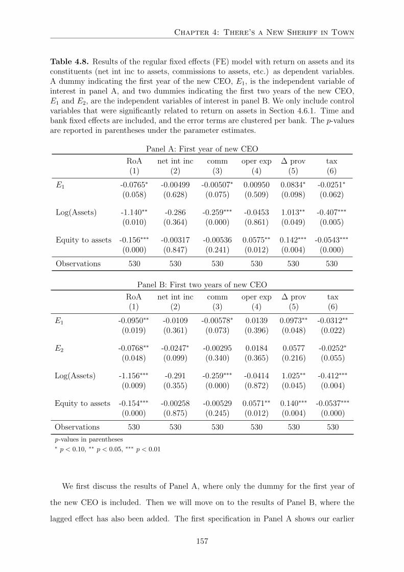
Chapter 4: There’s a New Sheriff in Town
Table 4.8. Results of the regular fixed effects (FE) model with return on assets and itsconstituents (net int inc to assets, commissions to assets, etc.) as dependent variables.A dummy indicating the first year of the new CEO, E1, is the independent variable ofinterest in panel A, and two dummies indicating the first two years of the new CEO,E1 and E2, are the independent variables of interest in panel B. We only include controlvariables that were significantly related to return on assets in Section 4.6.1. Time andbank fixed effects are included, and the error terms are clustered per bank. The p-valuesare reported in parentheses under the parameter estimates.
Panel A: First year of new CEO
RoA net int inc comm oper exp ∆ prov tax(1) (2) (3) (4) (5) (6)
E1 -0.0765∗ -0.00499 -0.00507∗ 0.00950 0.0834∗ -0.0251∗
(0.058) (0.628) (0.075) (0.509) (0.098) (0.062)
Log(Assets) -1.140∗∗ -0.286 -0.259∗∗∗ -0.0453 1.013∗∗ -0.407∗∗∗
(0.010) (0.364) (0.000) (0.861) (0.049) (0.005)
Equity to assets -0.156∗∗∗ -0.00317 -0.00536 0.0575∗∗ 0.142∗∗∗ -0.0543∗∗∗
(0.000) (0.847) (0.241) (0.012) (0.004) (0.000)
Observations 530 530 530 530 530 530
Panel B: First two years of new CEO
RoA net int inc comm oper exp ∆ prov tax(1) (2) (3) (4) (5) (6)
E1 -0.0950∗∗ -0.0109 -0.00578∗ 0.0139 0.0973∗∗ -0.0312∗∗
(0.019) (0.361) (0.073) (0.396) (0.048) (0.022)
E2 -0.0768∗∗ -0.0247∗ -0.00295 0.0184 0.0577 -0.0252∗
(0.048) (0.099) (0.340) (0.365) (0.216) (0.055)
Log(Assets) -1.156∗∗∗ -0.291 -0.259∗∗∗ -0.0414 1.025∗∗ -0.412∗∗∗
(0.009) (0.355) (0.000) (0.872) (0.045) (0.004)
Equity to assets -0.154∗∗∗ -0.00258 -0.00529 0.0571∗∗ 0.140∗∗∗ -0.0537∗∗∗
(0.000) (0.875) (0.245) (0.012) (0.004) (0.000)
Observations 530 530 530 530 530 530
p-values in parentheses∗ p < 0.10, ∗∗ p < 0.05, ∗∗∗ p < 0.01
We first discuss the results of Panel A, where only the dummy for the first year of
the new CEO is included. Then we will move on to the results of Panel B, where the
lagged effect has also been added. The first specification in Panel A shows our earlier
157

Drivers of Bank Performance and The International Cost of Equity
result of underperformance at a bank in the first year of a new CEO. This decline in
return on assets cannot be attributed to a decrease in net interest income or an increase
in operating expenses (see Specifications 2 and 4, respectively). The decrease in return
on assets is almost entirely explained by an increase in provisions (Specification 5).26
Although commissions also show a significant decrease (Specification 3), the economic
impact on return on assets is negligible, compared to the impact of ∆ provisions. The
results for the first year of a new CEO in Panel B are similar, but statistically stronger
than the results in Panel A. In the second year, the return on assets again shows a sig-
nificant decline. Although the decrease in net interest income is significant at the 10%
level, the decline in return on assets is again, for the largest part, caused by an increase
in provisions (even though the coefficient is statistically insignificant).
These results are in line with the finding of Jenter et al. (2016) that CEO turnover
has no impact on operating performance. They also undermine the argument that a
new CEO needs time to adapt and become acquainted with their new bank, for in such
a case, we would have expected a decrease in performance due to a material decline
in income or an increase in costs. Here, however, the decline in performance is almost
entirely caused by the increase in provisions for impaired loans, which is in line with the
finding of Bornemann et al. (2015) for German savings banks. This evidence suggests
that in their first year(s) in power, a new CEO classifies additional loans as impaired and
takes corresponding provisions to cover for expected losses. The final, sixth specification
indicates a significant decline in tax expenditure. This, however, is merely a mechanical
effect, since taxes automatically decline when earnings do.
The increase in provisions can be interpreted in the following two ways: departing
CEOs have been too lenient in provisioning for non-performing loans or new CEOs take
26We also want to check whether the decrease in return on assets and the increase in provisions can beexplained by a new CEO bringing in new clients. Therefore, in unreported regressions, we have addedasset growth as independent variable to Specifications 1 and 5 in the table above. Asset growth hasbeen chosen instead of loan growth since loans comprise 92% of the median bank’s assets. The resultsdo not materially change compared to the baseline specifications.
158

Chapter 4: There’s a New Sheriff in Town
an earnings bath in their first year. If the increase were due to departing CEOs being too
lenient, we would expect a negative relationship between the dummy in the last year(s)
of the departing CEO, E−1 and/or E0, and ∆ provisions. If, on the other hand, it is due
to CEOs taking an earnings bath, we expect the coefficient on dummies in subsequent
years to reverse. Therefore, we estimate regressions with ∆ provisions to assets as the
dependent variable and dummies equaling 1 in the last two years of the old CEO and the
first three years of the new CEO as main independent variables. Results are presented
in Table 4.9.
Table 4.9. Results of the regular fixed effects (FE) fixed effects model with ∆ provisionsto assets as the dependent variable and Eτ for τ ∈ {−1, 0, 1, 2, 3} as the main independentvariables. We only include control variables that were significantly related to return onassets in Section 4.6.1. Time and bank fixed effects are included, and the error termsare clustered per bank. The p-values are reported in parentheses under the parameterestimates.
τ = −1 τ = 0 τ = 1 τ = 2 τ = 3
Eτ -0.135∗∗ 0.0300 0.0834∗ 0.0284 -0.0681∗
(0.018) (0.439) (0.098) (0.558) (0.060)
Log(Assets) 0.970∗ 0.982∗ 1.013∗∗ 0.983∗ 0.963∗
(0.058) (0.057) (0.049) (0.053) (0.060)
Equity to assets 0.129∗∗∗ 0.141∗∗∗ 0.142∗∗∗ 0.141∗∗∗ 0.143∗∗∗
(0.006) (0.003) (0.004) (0.003) (0.003)
Observations 530 530 530 530 530
p-values in parentheses∗ p < 0.10, ∗∗ p < 0.05, ∗∗∗ p < 0.01
For τ = 1, the results are identical to the fifth specification in Panel A of Table 4.8:
that is, in the first year of the new CEO, there is a significant increase in provisions for
impaired loans. The insignificance of the dummy’s coefficient when τ = 0, representing
the last year of the departing CEO, shows that they were not more lenient in classifying
impaired loans in their final year. However, when we go back another year (τ = −1),
the second-to-last year of the predecessor, we do document a significant decline in provi-
sions. In unreported regressions, we found that this decline in provisions is paired with
159
Drivers of Bank Performance and The International Cost of Equity
an increase of similar size in return on assets in the second-to-last year.
Next, we assess whether the increase in ∆ provisions in the first year is reversed in
subsequent years. For the second year of a new CEO (τ = 2), we document an insignifi-
cant and slightly positive impact on provisions. A reversal takes place in the third year
(τ = 3), when provisions are significantly decreased by an almost equal amount as the
increase in the first year.
In sum, the increase in provisions in the first year of the successor occurs two years
after and two years before a significant decline in provisions. Therefore, the increase in
provisions in the first year of the new CEO seems to be induced by two forces. On the
one hand, it is the flipside of the decrease in provisions two years before the changeover,
and on the other, the new CEO takes an earnings bath which is subsequently offset in
the third year.27
4.7 Conclusion
The goal of this chapter is to establish the impact of CEO turnover on the financial
performance of banks. We documented that in the first year(s) of a new CEO, a bank’s
financial performance drops significantly. The return on assets decreases with 0.08 per-
centage points in the first year and 0.17 percentage points in the first two years, which
equals 23% and 50% of the standard deviation, respectively. This decline is not a con-
sequence of lagging interest income, a decrease in commissions, or a surge in operating
expenses, but can be attributed to an increase in provisions for impaired loans. The in-
crease in provisions in the first year of a newly appointed CEO is paired with a decrease
in provisions in the second-to-last year of the old CEO and in the third year of the new
27We remark that the combination of an increase in provisions in the first year of a new CEO, andsubsequently, a reversal in the third year, need not be a reflection of opportunistic behavior per se. Analternative interpretation could be that the new CEO wants to ensure that they will not be confrontedwith unforeseen bad loans in the future. Therefore, the successor increases the provisions in the firstyear, and, subsequently, when they become familiarized with the loan book, may discover that the initialprovisions were too conservative, which then leads to a decrease in these provisions.
160

Chapter 4: There’s a New Sheriff in Town
CEO.
We conclude from this that in their first year, a successor CEO wants to offset the
backlog in provisions inherited from their predecessor and/or ensure a position from
which to boost results – by decreasing provisions in the future. The decrease in per-
formance due to an increase in provisions is not without harm. Losses at banks reduce
their capital position and inhibit their ability to extend credit to customers. In addition
to these indirect effects, clients whose loans have been classified as impaired will become
subject to increased scrutiny from the bank, which might lead to additional costs for
both customer and bank.
161

Drivers of Bank Performance and The International Cost of Equity
162

5 | The World We Live In: Global
or Local?
Co-Authors: Jenke ter Horst, Kees Koedijk, and Ronald
Mahieu
Abstract
In this chapter, we document economically and statistically large differences
in the cost of equity by comparing a global CAPM to a local CAPM. We consider
fifteen countries over a nearly 20-year period (1996–2015). While the application
of the global version of the CAPM in cases where a global market index is used
as a pricing factor would seem justified by increased capital market integration,
the empirical evidence on this has been inconclusive to date. We found that the
average difference in the cost of equity between the models was equal to 0.77
percentage points, which represents about 20% of the historical risk premium.
Moreover, for almost 20% of the companies, this difference in cost of equity is
also statistically significant. For these companies the difference in cost of equity
is equal to 1.49 percentage points. We therefore conclude that not applying the
global CAPM but instead the local CAPM can lead to considerable mistakes in
cost-of-equity calculations.
163

Drivers of Bank Performance and The International Cost of Equity
5.1 Introduction
An important element in determining the cost of equity for individual companies is the
capital asset pricing model (CAPM). In theory, the global version of the model, the
ICAPM, should be used for integrated financial markets, since integration implies that
stocks are priced similarly across the board, irrespective of where they are traded. That
would make the global market index the most relevant index, and it should therefore re-
place the local indices used for cost of capital calculations in the traditional local CAPM.
The underlying empirical results have, however, been inconclusive to date.
This chapter presents an analysis of the cost of equity in global financial markets.
It builds on Koedijk, Kool, Schotman, and Van Dijk (2002) and Stulz (1995) in the
sense that it assesses whether there is a pricing error in the computation of the cost
of equity when a local CAPM is used even though the ICAPM applies. This pricing
error is especially interesting from a practical point of view, since the CAPM is still the
benchmark model in practice for calculating the cost of equity.1 The widespread use
of the CAPM has been demonstrated by Graham and Harvey (2001) for the U.S. and
Brounen, De Jong, and Koedijk (2004) for Europe.
This chapter uses the same methodology as Solnik (1974b) and Stulz (1995). Solnik
(1974b) reviewed nearly 300 stocks from nine developed countries and found a difference
in the cost of equity when the local CAPM was used despite the fact that the ICAPM
applied for more than 50% of the companies. Stulz (1995) took this into greater detail,
limiting his analysis to Nestle, and documented an economically large difference. In
Koedijk et al. (2002), the approach of Solnik (1974b) and Stulz (1995) was extended by
1Acquaintances working for international investment banks told us that the CAPM is still the bench-mark model for computing the cost of equity. At one bank, they always use the local CAPM model, andat another, it depends on whether the company in question operates primarily locally or globally. Forcompanies operating globally, the cost of equity is then computed with a global version of CAPM. Fi-nally, investment banks often use Damodaran data sets (http://pages.stern.nyu.edu/~adamodar/)to find a company’s beta. The definitions for the variables in those data sets state that the beta iscomputed using a local CAPM, where the index is “the most widely followed index in the market.”
164

Chapter 5: The World We Live In: Global or Local?
adding exchange rates as pricing factors in the model. Their sample consisted of 3,293
stocks in nine countries. Overall, Koedijk et al. (2002) found that for many companies
in their sample, it did not matter whether the global or local CAPM was used. Applying
an alternative method and focusing exclusively on the U.S., Harris, Marston, Mishra,
and O’Brien (2003) also concluded that it did not matter much for the cost-of-equity
computation whether the local or global market model was used. Moreover, Jacquillat
and Solnik (1978) had previously concluded that adding other major markets on top of
the home market often does not yield any improvement in explaining the stock returns
of multinational firms. While this result is consistent with the findings of Koedijk et al.
(2002), it must be treated with care, since the developed markets at the time were not
yet integrated.
In sum, the empirical evidence thus far has been inconclusive. The culmination of
capital market integration in developed countries in the 1990s (Bekaert, Harvey, Lund-
blad, & Siegel, 2011), which is a basic assumption in our model, presents us with a
20-year time period for assessing the impact on the cost of equity of using a local in-
stead of a global model. Moreover, the increasing capital market integration of emerging
markets (Bekaert & Harvey, 2003; Carrieri, Chaieb, & Errunza, 2013) justifies extending
the analysis to emerging markets. Our results show that over the entire period we focus
primarily on, 1996–2015, the difference in cost of equity when using the local CAPM
despite applicability of the ICAPM was equal to 0.77 percentage points. This represents
18% of the historical risk premium.2 Moreover, on average for 19% of the companies in a
country, this difference is also statistically significantly distinct from zero. Furthermore,
this percentage differs considerably between countries, ranging from 1.9% for China to
63% for Switzerland. When focusing exclusively on companies for which the difference
is significantly different from zero the mistake in cost of equity jumps from 0.77 to 1.49
percentage points – equal to 35% of the historical risk premium. This implies that not
2The equity risk premium for a U.S. investor on the global market for the period 1900-2015 is equalto 4.2% (Credit Suisse, 2016, pg. 61). Therefore, a mistake in cost of equity of 0.77 percentage pointsrepresents 0.77%/4.2%=18% of the global equity risk premium.
165

Drivers of Bank Performance and The International Cost of Equity
using the ICAPM but instead the local CAPM in cost of equity calculations can lead to
considerable mistakes.
The previous discussion does not distinguish between an under- and overestimation
of the cost of equity. The implications are, however, the exact opposite. Using the
Gordon growth model, where the stock price represents the discounted stream of future
dividends and the discount rate equals the ‘real’ cost of equity (Gordon, 1962; Gordon
& Shapiro, 1956; Williams, 1938), any underestimation of the cost of equity implies an
overvaluation of the company. This, in turn, could result in overinvestment by that com-
pany. In our sample, this situation occurs in Switzerland. Conversely, overestimation of
the cost of equity leads to the undervaluation of a company.
For fourteen of the fifteen countries we considered, it made a difference for at least
5% of the sample companies whether the ICAPM or local CAPM was used. Remark-
ably, this was not the case for China, where only 1.9% of the sample companies had
errors that were significantly different from zero. We ascribe this to the segmentation of
the Chinese capital market in general and the overrepresentation in our sample of small
Chinese stocks, which are particularly likely to be more segmented.
As a robustness check we extended the global pricing model by adding the Fama-
French factors. Since we only have data on the Fama-French factors for North America
and Europe, we could not perform this analysis for all countries. However, for the ma-
jority of the countries for which we did have that data, there is a slight increase in the
number of companies for which the cost of equity differs significantly when the local
model is used even though the global model applies when that data is added in. There-
fore, we conclude that our results are robust for this more general specification.
The chapter proceeds as follows. Section 5.2 discusses the integration of capital
markets. In Section 5.3, we explain our methodology, while Section 5.4 describes the
166

Chapter 5: The World We Live In: Global or Local?
data. In Section 5.5, we present the results and in Section 5.6, we show the robustness
of our results for an alternative model. Finally, we present our conclusions in Section
5.7.
5.2 Capital Market Integration and the Cost of Eq-
uity
Stulz (1995) assumes integration of capital markets throughout his analysis of the dif-
ference in cost of equity when using a local versus a global market index. He argues
that the internationalization of capital markets has made the use of the local CAPM
inappropriate, especially for small countries. In the twenty years that have passed since
Stulz published his findings, the globalization of the world economy has only accelerated,
as reflected for instance by the increasing prominence of emerging markets in the world.
There is much academic research focusing on market integration in general and the
developments in the emerging markets in particular. According to Bekaert et al. (2011),
the local markets of developed countries were integrated with global markets as of 1993,
although emerging markets are still segmented. This segmentation persists despite an
increase in capital flows to emerging markets throughout the 1990s (Bekaert & Harvey,
2003). The authors link this increase in capital flows to the liberalization of capital
markets in emerging markets.
Carrieri et al. (2013) start with a theoretical approach to integration, which was de-
veloped by Errunza and Losq (1985), drawing a distinction first between integrated and
segmented markets and subsequently within segmented markets between accessible and
non-accessible securities. The former are securities in which international investors can
invest, while the latter are isolated from international investors. Markets with securi-
ties shielded from foreign investors are not fully integrated with world capital markets.
Therefore, these segmented securities have a global market risk premium and a local risk
167

Drivers of Bank Performance and The International Cost of Equity
premium, whereas integrated securities only have a global risk premium. An example of
such a situation is China, where A shares are only available to domestic investors, while
B shares can be acquired by both domestic and foreign investors.
When they compare their model with the data, Carrieri et al. (2013) show that the
markets of developed economies are integrated with global capital markets. Further-
more, in emerging markets, stocks that are accessible to all investors are integrated with
capital markets and hence only have global market risk. However, stocks that are not
accessible to all investors have not only global market risk, but also local market risk.
Whether emerging markets in the aggregate are characterized more as integrated or
segmented then depends on the relative importance of accessible versus non-accessible
stocks. Nevertheless, there appears to be consensus that the segmentation of emerging
markets is decreasing over time (Bekaert & Harvey, 2003; Carrieri et al., 2013).
Despite evidence that capital markets are becoming increasingly integrated, there are
still barriers to integration. Bekaert and Harvey (2003) distinguish between three types
of barriers: legal, indirect, and emerging-market specific. Legal barriers make it difficult
or unattractive for foreign investors to invest in a country. These include such things
as restrictions on foreign ownership or additional taxes for foreigners. Indirect barriers
refer to differences in the level of information available to domestic and foreign investors,
unfamiliar accounting standards, and limited protection for small investors. This is
corroborated by Carrieri et al. (2013), who point specifically to the quality of information,
the institutional environment, and corporate governance standards as factors hindering
the integration of emerging markets. A theoretical exposition of how the expropriation
of outsiders (including foreign investors) by corporate insiders and sovereign states leads
to segmentation is provided by Stulz (2005). Finally, emerging markets have specific
risks related to liquidity, politics, and economic policy. In sum, it is safe to assume that
financial market integration is justifiable for developed countries. For emerging markets,
however, although they are increasingly integrated with world capital markets, there
168

Chapter 5: The World We Live In: Global or Local?
still remain barriers to integration. This should be kept in mind when we interpret our
empirical results.
5.3 Methodology
Similar to Stulz (1995), we use the CAPM of Grauer, Litzenberger, and Stehle (1976),
in which the market factor is the only factor in the asset pricing model. In this model,
purchasing power parity is assumed [or deviations are not large enough to impact asset
prices (Stulz, 1995)] and therefore exchange rate risk is not priced. It is possible to ex-
tend the model to the Solnik-Sercu model (Sercu, 1980; Solnik, 1974a), which allows for
exchange rate risk to be priced. For our purposes, however, since it is unclear whether
exchange rate risk is priced or not (Bekaert & Hodrick, 2009, p. 451), we will use the
simple CAPM model.3
In deriving our testable hypothesis we follow the set-up of Koedijk et al. (2002) and
Stulz (1995). Let Ri be a vector of length T of total returns in U.S. dollars on individual
stocks i ∈ {1, ..., N}. RG is a vector of length T of total returns on a global equity
market index, measured in U.S. dollars. The ICAPM can be written as
E[Ri] = αG,i + βG,iE[RG], (5.1)
where βG,i = Cov[Ri,RG]V ar[RG]
(e.g., Bekaert & Hodrick, 2009, pp. 446–447). Since we assume
integration of capital markets, this is the correct model to compute the cost of equity.
We choose the CAPM representation that includes the riskless interest rates in the αG,i
term. This representation of asset prices is the maintained hypothesis throughout the
chapter.
The local CAPM model is similar to Equation (5.1), with the global equity market
3Dumas and Solnik (1995) show that the exchange rate risk for Germany, the U.K., Japan, and theU.S. is priced, while Griffin and Stulz (2001) conclude that exchange rate shocks have only a smallimpact on stock returns. For an excellent overview of alternative asset pricing models in global financialmarkets, we refer readers to Karolyi and Stulz (2003).
169
Drivers of Bank Performance and The International Cost of Equity
index replaced by a local one, written as RL. The local CAPM is given by
E[Ri] = αL,i + βL,iE[RL],
where βL,i = Cov[Ri,RL]V ar[RL]
and αL,i incorporates the riskless rates terms. This would be
the correct model to determine the cost of equity if capital markets would have been
segmented. However, even though we assume integrated markets, the local CAPM does
not necessarily lead to a significant difference in cost of equity compared to the ICAPM.
The main goal of this chapter is to determine when this difference is significant. In the
remainder of this section, we will derive a testable hypothesis to test the significance of
this difference.
Since βG,i and βL,i coincide with the regression coefficients of regressing Ri on RG
and RL, respectively, we can write
Ri = αG,i + βG,iRG + εG,i, (5.2)
and
Ri = αL,i + βL,iRL + εL,i, (5.3)
where εG,i and εL,i have mean zero and are orthogonal to RG and RL, respectively (see
Appendix A.1 for a derivation of the orthogonality between εG,i and RG).
Given that the ICAPM is the maintened hypothesis throughout the chapter, it should
also hold for the return on the local index, RL; that is,
E[RL] = αG,L + βG,LE[RG].
Similar to Equations (5.2) and (5.3), we obtain:
RL = αG,L + βG,LRG + εG,L, (5.4)
where εG,L has mean zero and is orthogonal to RG.
170

Chapter 5: The World We Live In: Global or Local?
Inserting this expression into Equation (5.3), we get
Ri = αL,i + βL,i (αG,L + βG,LRG + εG,L) + εL,i
= αL,i + βL,iαG,L + βL,iβG,LRG + βL,iεG,L + εL,i. (5.5)
If the ICAPM holds, εG,L is orthogonal toRG and Equations (5.2) and (5.5) are equivalent
if and only if local idiosyncratic risk εL,i is orthogonal to RG. In that case, the parameters
of Equations (5.2) and (5.5) corresponding to the risk factors should be equal, such that
βG,i = βL,iβG,L. (5.6)
To test for orthogonality between εL,i and RG, we consider the following regression
equation:
εL,i = κiRG + ηi, (5.7)
where κi is the parameter for the global index, and ηi has mean zero and is orthogonal
to RG and RL. In the bivariate case with only one independent variable, the regression
anatomy formula presented in Angrist and Pischke (2009, pg. 27), which they ascribe
to Frisch and Waugh (1933), implies:
κi =Cov[εL,i, RG]
V ar[RG]=E[ε′L,i ·RG]
V ar[RG],
where the second equality holds because E[εL,i] = 0. Our null hypothesis then is that
the part of the return not accounted for by the local index (i.e., εL,i) is orthogonal to the
global index. In other words, the global index cannot explain the return development of
asset i any better than the local index. This would imply that no error is made by using
the local CAPM instead of the ICAPM, and thus the pricing error equals zero.
To test for differences in the cost of equity when using the local versus the global
171

Drivers of Bank Performance and The International Cost of Equity
index, we insert Equation (5.7) in Equation (5.3) to arrive at
Ri = αL,i + βL,iRL + κiRG + ηi, (5.8)
where ηi has mean zero and is orthogonal to RG and RL (see Appendix A.2 for a deriva-
tion of this result). This equation is similar to Equation (8) of Koedijk et al. (2002).
We use a t-test to test at the 5% level whether the coefficient for the global index, κi, is
equal to zero. This will be tested per company.4
The derivations above are based on the assumption that capital markets are fully
integrated. At the end of Section 5.2, we concluded that this is a valid assumption for
developed countries but not for developing ones. Caution is therefore advised in applying
the aforementioned framework to emerging markets. Intuitively, the more segmented
markets are, the more important local factors will be in explaining a firm’s stock return,
and hence the more likely it will be that the global factors will not add much information.
Therefore, the local factor, RL, will explain much of the firm’s stock return for a company
segmented from world markets. This implies that the global factor, RG, will be less
relevant and hence the corresponding coefficient κi will often be close to zero. The results
are presented and discussed later in the chapter, where we focus first on the statistical
significance of the difference between using the local CAPM versus the ICAPM (Section
5.5.1), before assessing whether this difference is also economically significant (Section
5.5.2).
5.4 Data
In our sample, we consider the world’s thirteen largest economies (not including Italy),
plus the Netherlands and Switzerland. Italy was left out of the sample because we did
not have access to the index constituents of the past, and the latter two countries were
included because Dutch and Swiss multinational companies sell a large share of their
4This set-up assumes that the sample companies are independent observations. An interesting ex-tension of this approach would be to allow for correlation between stock returns of the companies.
172

Chapter 5: The World We Live In: Global or Local?
products abroad (Jacquillat & Solnik, 1978), which is an interesting setting to test our
hypothesis. This amounts, then, to eleven developed countries and the BRIC (Brazil,
Russia, India, and China) countries. The starting point for the selection process in
choosing the companies per country was the major index in that country, where we iden-
tified all of the constituents (i.e., every company that appeared at least once in the index
from 1980 to 2015) and used this as our sample of firms.5 In addition to our sample of
firms, we also collected data on the local market indices from the sample countries and
the global market index.6 Share prices and market indices are recorded at a monthly
frequency from Datastream, and dividends are reinvested. In the rest of the chapter,
we focus on the period from January 1996 to June 2015. Our time period starts a few
years after developed markets were considered fully integrated with global markets [i.e.,
1993, the date given by Bekaert et al. (2011)]. A complete overview of the data and the
sources can be found in Appendix B.
At this point, it is important to mention that throughout this chapter, we adopt
the perspective of a U.S. investor. Consistency therefore requires that all returns be
converted into U.S. dollar returns. It was not possible, however, to download the local
MSCI index for Russia or China in U.S. dollars. To overcome this problem, we converted
both of these indices, which were initially denominated in the local currencies, into U.S.
dollar amounts using exchange rate data from Datastream (Russia) and FRED7 (China).
Table 5.1 contains an overview of the stocks in our sample.
5For Australia, we could only download the constituents for May and June 2015.6The local market for Russia starts on May 1, 1996.7Federal Reserve Economic Data, Federal Reserve Bank of Saint Louis, https://research
.stlouisfed.org/fred2/.
173

Drivers of Bank Performance and The International Cost of Equity
Table 5.1. The second column contains the number of companies per country in theraw dataset that had at least one observation in the period 1996–2015. Columns 3, 4,and 5 contain the number of companies listed for the periods 1996–2015, 1996–2005, and2006–2015, respectively. In the third to fifth columns, companies have been excludedfor which one of the following applies: 1) there are not at least 12 observations; 2)stock returns are equal to zero for more than 20% of the observations; or 3) the averageannual return is over 200%.
Country # sample # sample # sample # samplestocks stocks stocks stocks
1996–2015 1996–2005 2006–2015
Australia 332 326 272 266Canada 538 530 443 474France 242 238 207 192Germany 1,010 985 857 780Japan 209 207 195 205The Netherlands 58 57 47 52Spain 71 69 58 63South Korea 200 114 82 132Switzerland 76 76 66 76United Kingdom 1,869 1,819 1,570 1,122United States 1,033 1,013 954 774
Brazil 111 109 69 109Russia 90 88 30 89India 74 74 62 74China 1,706 1,603 567 1,596
Total 7,657 7,345 5,509 6,041
In Column 2, we report the number of stocks per country, as determined by taking
all of the companies included in the country’s major stock exchange (see Column 2 of
Table B.1 for these indices) between 1980 and 2015 that have also had at least one stock
return in the period 1996–2015.8
Next, following Koedijk et al. (2002), we imposed the following restrictions on this
8In the first step, we used the constituents of the index to identify companies that had at one pointbeen listed from 1980 to 2015. We then excluded companies which had been delisted before the startof our sample period, i.e., 1996. For example, a company which was in the index in 1985 but delistedin 1988 was excluded from the sample, whereas one that was in the index in 1985 but delisted in 1997was included.
174

Chapter 5: The World We Live In: Global or Local?
raw dataset. First, we required that there be at least twelve monthly observations for
each company. Second, over the period for which the stocks are listed, each company
must have had fewer than 20% zero-return observations. Third, the average annual re-
turn must not exceed 200%.9 The number of companies satisfying these conditions is
shown in Column 3 of Table 5.1.
In Columns 4 and 5, we restrict the full sample to stocks that had a listing in 1996–
2005 and 2005–2015, respectively. The number of companies in Columns 4 and 5 is lower
or equal to the number in Column 3 as a result of delistings and new listings from 1996
to 2015. The restrictions mentioned previously were also applied to the two 10-year
sub-periods.
We point to two patterns in Table 1. First, there were many new listings in the BRIC
countries from 1996 to 2015. This can be inferred from the difference between Columns 3
and 4. Moreover, only a few companies were delisted in this period, as inferred from the
difference between Column 5 and Column 3.10 This is a reflection of the development of
these countries’ capital markets in this period.
Second, for the developed economies, a considerable number of companies were
delisted during the first sub-period. This is particularly true for the U.K. and the
U.S., where 38% and 23%, respectively, of the companies listed at one point during
the 1996–2015 period were delisted. This is confirmed by the World Development In-
dicators (WDI) from the World Bank (see http://data.worldbank.org/indicator/
CM.MKT.LDOM.NO?view=chart), which show a peak in listings in 1996 for the U.S. and
in 2006 for the U.K.11
9To arrive at the average annual return, we took the monthly mean return plus one to the power oftwelve minus one, Rannual = (1 + Rmonth)12 − 1. In cases where this number exceeded 2 (200%), thecompany was excluded from the sample.
10A comparison of these columns does not give an exact number of new listings and delistings, dueto the restrictions applied on each individual period.
11For a discussion about the reasons why the U.S. lags behind in terms of company listings, seeDoidge, Karolyi, and Stulz (2017).
175
Drivers of Bank Performance and The International Cost of Equity
5.5 Results
The results section comprises three subsections. We first test whether there are statisti-
cally significant differences in the cost of equity when we use the local CAPM even though
the ICAPM applies. Next, we assess how large the differences in the cost-of-equity levels
are, whereby we make a distinction between companies with or without a statistically
significant different cost of equity. Finally, we graphically depict the differences.
5.5.1 Difference in Cost of Equity
In this section, we assess whether the cost of equity differs significantly when we use
the ICAPM versus the local CAPM. In Table 5.2, we present the rejection rates per
country. Rejection takes place for company i when κi from Equation (5.8) is significantly
different from zero. This means that in these cases, the cost of equity using the ICAPM
is significantly different from that when using the local CAPM. The rejection rate is
the number of sample companies in a country for which the null is rejected in relation
to the total number of sample companies in that same country. For each country, we
consider the full time period, 1996–2015, and the two sub-periods, 1996–2005 and 2006–
2015, which both cover 10 years. In estimating the regression equations, we account for
heteroskedasticity.12
12Since our data is on a monthly frequency, autocorrelation is less of a concern.
176

Chapter 5: The World We Live In: Global or Local?
Table 5.2. The percentage of rejection compared to the total number of companies inour sample per country per time period. Rejection occurs when the coefficient of theglobal market in Equation (5.8) is significantly (at the 5% level) different from zero. At-test is applied to test this hypothesis.
1996–2015 1996–2005 2006–2015
Australia 17% 14% 16%Canada 24% 11% 25%France 11% 8.7% 14%Germany 10% 10% 7.4%Japan 34% 27% 26%The Netherlands 26% 17% 21%South Korea 7% 7.3% 16%Spain 19% 14% 24%Switzerland 63% 42% 49%United Kingdom 19% 20% 15%United States 15% 14% 15%
Brazil 22% 7.3% 19%Russia 11% 0% 11%India 11% 6.5% 18%China 1.9% 3.2% 2.4%
First, focusing on the full period, we conclude that of the developed countries all
have rejection rates above 5%. This means that the cost of equity changes significantly
when the local CAPM is used despite applicability of the ICAPM for 7% to 63% of
companies depending on the country. The most extreme case is Switzerland, where 63%
of the companies in the full period show a significant difference in the cost of equity.
This is consistent with the results of Jacquillat and Solnik (1978), who document a large
increase in explaining Swiss stock returns when other market indices are added to the
Swiss index. In sum, we conclude that whether or not the local CAPM is used even
though the ICAPM applies often makes a difference in the computation of the cost of
equity.
Second, China is an anomaly in the sense that its rejection rate is the lowest of all of
the countries (both developed and emerging). Moreover, the rejection rate remains below
5% in the two sub-periods. Comparing China to the other BRICs, we see that its rejec-
177

Drivers of Bank Performance and The International Cost of Equity
tion rates are generally lower, especially for the full period and the second sub-period.
Hence, there seems to be something special about China. From the market integration
section, we know that emerging markets are less integrated in general than developed
markets. Although this argument applies for all emerging markets, and not just China,
it is more relevant for China than for others for two reasons. First, many Chinese com-
panies are not accessible to foreign investors, and second, these non-accessible companies
are less integrated with world capital markets than the non-accessible companies of the
other BRICs (Carrieri et al., 2013). For companies which are less integrated with the
world market, the local index contains the most relevant information, resulting in low
rejection rates [see Equation (5.8)].
Third, the zero rejection rate for Russia in the first sub-period is peculiar. However,
we need to treat this percentage with care, because it is based on only 30 companies, for
which firm-level stock returns were only available in 55% of the months on average.
Finally, comparing the rejection rates of the two 10-year sub-periods, we conclude
that for eleven of the fifteen countries the rejection rate increases from the first to the
second sub-period, while it decreases for four countries. This highlights the increasing
importance of using the ICAPM instead of the local CAPM.13
5.5.2 Size of Difference in Cost of Equity
In the second part of this section, we want to assess the size of the difference in cost
of equity when the local CAPM is used even though the ICAPM applies. To quantify
13The rejection rates for the full period are either in between the rates for the two sub-periods orhigher than both. There are two dynamics at work here. On the one hand, combining the two sub-periods into one full period averages the rates over both sub-periods. On the other hand, the numberof observations per company is higher for the full period than for individual sub-periods, leading to anincrease in the power of the t-test. Hence, for countries where the rejection rate is higher for the fullperiod than for the sub-periods, the latter effect is strongest, while for the others, the former effectdominates. This reasoning applies when the set of companies in the different time periods is the same.Since newly listed companies enter the set and delisted companies leave, the set changes. This explainshow the rejection rate of South Korea and China for the full period could be lower than for eithersub-period.
178

Chapter 5: The World We Live In: Global or Local?
the size of the mistake at issue, we adopt Equation (5) of Stulz (1995) and inserted the
parameter estimates for the betas [see Equations (5.2), (5.3) and (5.4)], which yielded
the following equality:
Ri,G − Ri,G,L =(βG,i − βL,iβG,L
)(E[RG]− rf
), (5.9)
where E[RG] is the expected return on the global index in U.S. dollars and rf the risk-
less rate earned on U.S. T-bills. We use U.S. dollar returns and U.S. T-bills because we
assume the perspective of a U.S. investor. In other words, E[RG] − rf is equal to the
equity risk premium (ERP) of the global index in U.S. dollar returns.
Table 5.3 lists the absolute difference in cost of equity relative to the equity risk pre-
mium for each country when the local CAPM is used despite applicability of the ICAPM:
in other words, the value from Equation (5.9) divided by the equity risk premium. We
computed this relative difference in cost of equity for both “Reject” and “Non-reject”
companies. Reject companies are the ones for which the difference in cost of equity is
statistically significant, while Non-reject refers to companies for which this difference is
insignificant (see Section 5.5.1).
179

Drivers of Bank Performance and The International Cost of Equity
Table 5.3. The absolute average difference in cost of equity relative to the globalequity risk premium when the local CAPM is used even though the ICAPM applies.Results are presented per country. Companies for which the cost-of-equity differencewas statistically different at the 5% level (i.e., designated as “Reject”) were consideredseparately from companies for which the difference was insignificant (i.e., “Non-reject”)(see Section 5.5.1). The countries and two categories are listed in the first column. Thefigures presented in the second column equal the value from Equation (5.9) divided bythe global equity risk premium. We used the parameter estimates for the full period,1996–2015. The unweighted average of all the countries is presented in the bottom rows.
Country Difference
AustraliaReject 41%Non-reject 14%
CanadaReject 35%Non-reject 17%
FranceReject 27%Non-reject 10%
GermanyReject 37%Non-reject 14%
JapanReject 27%Non-reject 10%
The NetherlandsReject 35%Non-reject 15%
SpainReject 36%Non-reject 13%
South KoreaReject 38%Non-reject 15%
SwitzerlandReject 27%Non-reject 9.3%
United KingdomReject 37%Non-reject 26%
United StatesReject 15%Non-reject 12%
BrazilReject 33%Non-reject 9.9%
RussiaReject 46%Non-reject 19%
IndiaReject 33%Non-reject 12%
ChinaReject 63%Non-reject 22%
AverageReject 35%Non-reject 15%
Not surprisingly, we see across the table that the difference in cost of equity is larger
180
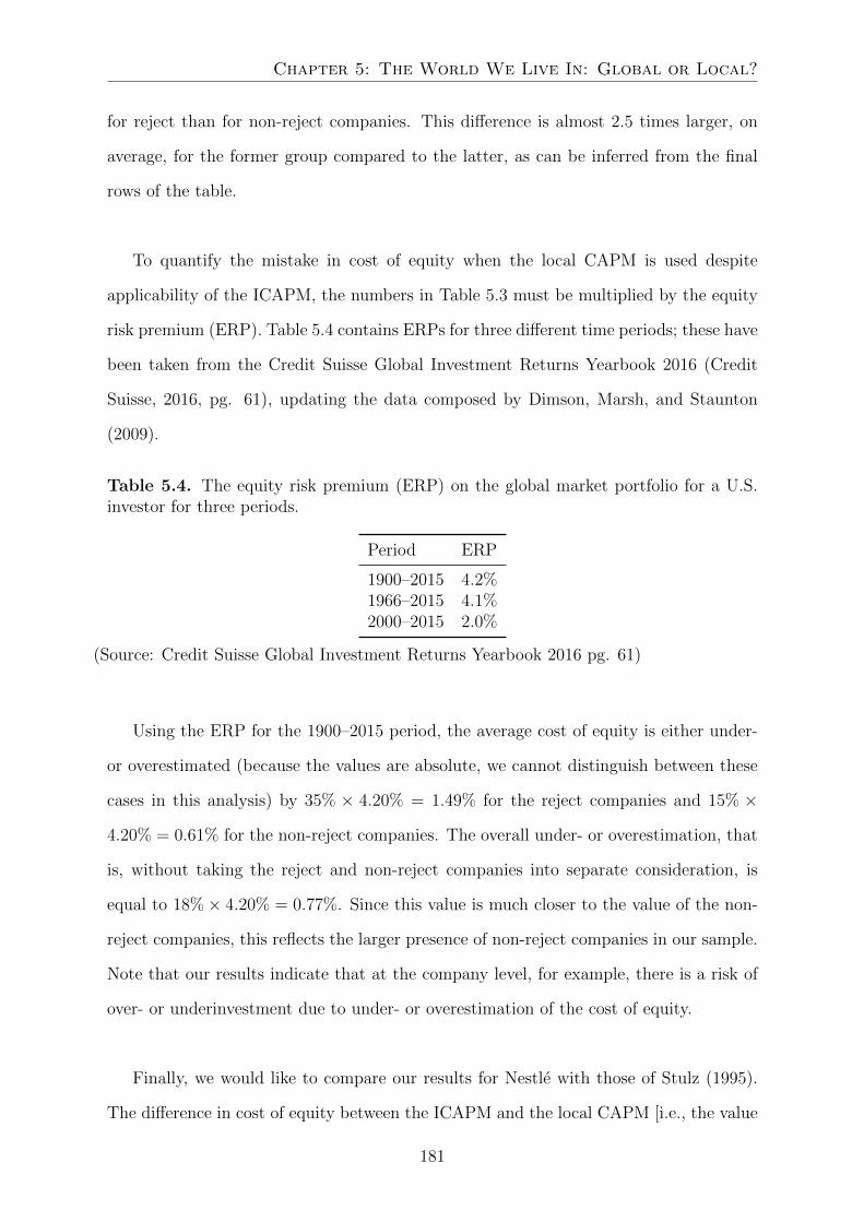
Chapter 5: The World We Live In: Global or Local?
for reject than for non-reject companies. This difference is almost 2.5 times larger, on
average, for the former group compared to the latter, as can be inferred from the final
rows of the table.
To quantify the mistake in cost of equity when the local CAPM is used despite
applicability of the ICAPM, the numbers in Table 5.3 must be multiplied by the equity
risk premium (ERP). Table 5.4 contains ERPs for three different time periods; these have
been taken from the Credit Suisse Global Investment Returns Yearbook 2016 (Credit
Suisse, 2016, pg. 61), updating the data composed by Dimson, Marsh, and Staunton
(2009).
Table 5.4. The equity risk premium (ERP) on the global market portfolio for a U.S.investor for three periods.
Period ERP
1900–2015 4.2%1966–2015 4.1%2000–2015 2.0%
(Source: Credit Suisse Global Investment Returns Yearbook 2016 pg. 61)
Using the ERP for the 1900–2015 period, the average cost of equity is either under-
or overestimated (because the values are absolute, we cannot distinguish between these
cases in this analysis) by 35% × 4.20% = 1.49% for the reject companies and 15% ×
4.20% = 0.61% for the non-reject companies. The overall under- or overestimation, that
is, without taking the reject and non-reject companies into separate consideration, is
equal to 18%× 4.20% = 0.77%. Since this value is much closer to the value of the non-
reject companies, this reflects the larger presence of non-reject companies in our sample.
Note that our results indicate that at the company level, for example, there is a risk of
over- or underinvestment due to under- or overestimation of the cost of equity.
Finally, we would like to compare our results for Nestle with those of Stulz (1995).
The difference in cost of equity between the ICAPM and the local CAPM [i.e., the value
181

Drivers of Bank Performance and The International Cost of Equity
of Equation (5.9)] he reported for Nestle was equal to –0.60%, while in our case it is
equal to between –0.27% and –0.13%, depending on which risk premium from Table 5.4
we use. Moreover, this difference is not significantly different from zero. We therefore
conclude that for Nestle, the overestimation of riskiness has decreased in the last twenty
years.14 This implies, for this particular case, that when the local CAPM was used, the
undervaluation of the stock price was lower than before. In addition, underinvestment
due to an overestimation of the discount rate has become less of a concern.
5.5.3 Illustration of Difference in Cost of Equity
To illustrate the differences in cost of equity when the local CAPM is used despite
ICAPM applicability, Figure 5.1 graphically depicts the direct and indirect betas per
company for the 1996–2015 period. The results are presented per country.
Each dot in the graph represents a company. In cases where there is no difference in
the cost of equity using the ICAPM versus the local CAPM the following equality [see
Equation (5.6)] should hold:
βG,i = βL,iβG,L.
In the figures, the x-coordinate is the estimate for the direct beta, βG,i, and the y-
coordinate is the estimate for the indirect beta, βL,iβG,L. In general, a pricing error is
small when a dot is close to the 45° line; conversely, the pricing error is large when a dot
is far from the line.
14Even if we had used the risk premium of 6.22% that Stulz (1995) uses, the difference would be–0.40%, which is still lower than the difference reported in Stulz (1995).
182
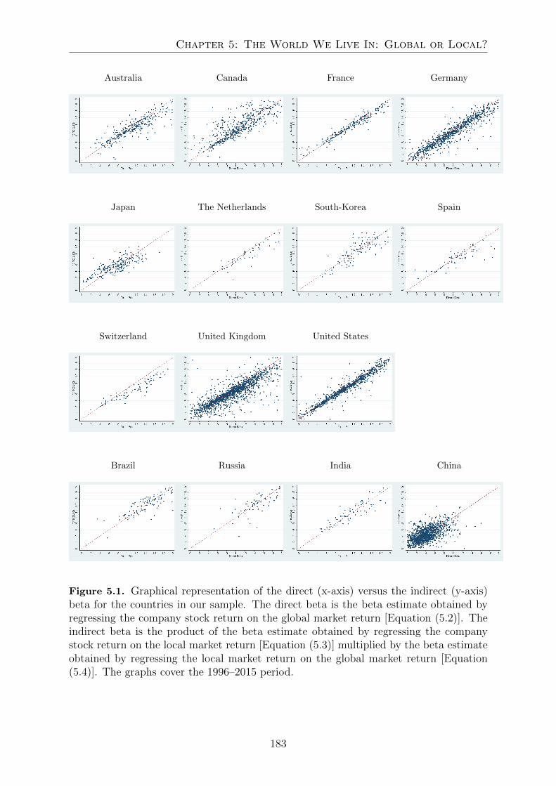
Chapter 5: The World We Live In: Global or Local?
Australia Canada France Germany
Japan The Netherlands South-Korea Spain
Switzerland United Kingdom United States
Brazil Russia India China
Figure 5.1. Graphical representation of the direct (x-axis) versus the indirect (y-axis)beta for the countries in our sample. The direct beta is the beta estimate obtained byregressing the company stock return on the global market return [Equation (5.2)]. Theindirect beta is the product of the beta estimate obtained by regressing the companystock return on the local market return [Equation (5.3)] multiplied by the beta estimateobtained by regressing the local market return on the global market return [Equation(5.4)]. The graphs cover the 1996–2015 period.
183

Drivers of Bank Performance and The International Cost of Equity
Before discussing individual countries, we would like to first discuss how to interpret
the graphs. Equation (11) of Stulz (1995) states that the market-value weighted-average
difference in cost of equity when using the local CAPM versus the ICAPM equals zero.
Note that this equality only holds when market indices include all stocks and their weight
in the index is weighted with market value. Although the latter condition has been sat-
isfied, since we only consider MSCI indices and those use market weighting, the former
condition is violated, since not all stocks are included in the MSCI indices.
Nevertheless, this does not seem to result in large distortions in our sample, since
the dots in the graphs are generally well situated around the 45° line. Differences in cost
of equity may occur for individual stocks, however, as can be concluded from the large
distance to the line for some of the dots. For these companies, a large error is introduced
when the local CAPM is used instead of the ICAPM. The placement of the dots above
or below the line determines whether the cost of equity is over- or underestimated. Dots
situated below the line have a higher cost of equity when using the ICAPM versus the
local CAPM. In other words, for this group, risk that is diversifiable locally is not di-
versifiable globally. Consider a firm whose return is uncorrelated with that part of the
local market which is globally diversifiable. This leads to a low local beta, βL,i. If, at the
same time, the firm’s return is strongly correlated with the world market, this results
in a large global beta, βG,i. The opposite holds for dots situated above the line: risk
that is diversifiable globally is not diversifiable locally. Note that overestimation – dots
above the line – leads to an undervaluation of the company or to underinvestment by
the company. Conversely, underestimation – dots below the line – leads to overvaluation
or overinvestment by the company.
To clarify the interpretation of the graph, we discuss the case of Switzerland. The
companies listed in that country are almost exclusively located below the line. This
implies an underestimation of the cost of equity when the local CAPM is used even
though the ICAPM applies. In other words, these companies are exposed to risk that is
184

Chapter 5: The World We Live In: Global or Local?
diversifiable locally and not globally. Knowing that the market-value weighted-average
of the differences for each country should be equal to zero, the subsample of Swiss firms
we consider is not representative, because the companies are all below the line. Hence,
the returns of Swiss firms in our sample are more correlated with the world market than
with the local market. A possible explanation for this could be that these firms operate
more globally. Moreover, from an investment perspective, the underestimation of the
cost of equity for these Swiss sample companies suggests an overvaluation of their stock.
Therefore, if an investor believes in the applicability of the ICAPM and expects market
participants to adopt the same belief instead of them applying the local CAPM, they
should short or underweight the Swiss sample companies in their portfolio.
Second, we look at the position of the dots along the 45° line. We focus first on Brazil
and Russia, and then on China, because the dots in these graphs are more clustered near
specific beta values. The Brazilian and Russian companies are congregated in the upper
right corner, while Chinese companies are grouped in the lower left corner. To explain
the position of the dots in these cases, we use a company’s indirect beta. This is the
product of the company’s beta in relation to the local market multiplied by the local
market’s beta in relation to the global market. Assuming that we have a representative
sample of companies for a country and that the local market index represents the local
market, we know that the companies within a country have a weighted average beta that
should be around one when the company return is regressed on the local index. In that
case, the clustering of indirect betas in certain regions of the graph is due to a high or
low beta for the local index in relation to the world index. This beta can be written as
follows:
βG,L =Cov[RG, RL]
V ar[RG]=ρG,L · σLσG
, (5.10)
where G and L denote global and local, respectively, and ρG,L is the correlation between
the return on the global and local index. Since the volatility, σG, of the global market
is the same for all countries, high betas are a result of either high volatility in the local
185
Drivers of Bank Performance and The International Cost of Equity
index or a high correlation between the local and the global market.
For Brazil and Russia, many of the dots are clustered in the upper right corner of
the graph. In Brazil’s case, this can be explained by a combination of a not-so-low cor-
relation between the Brazilian market and the world market, at 0.72 (the average for all
the countries is 0.76), and a relatively high local market volatility of 0.107 (the average
for all the countries is 0.078). For Russia, the high volatility of the local market, by far
the largest in the sample, at 0.159, explains the position of the Russian firms in the graph.
The volatility of the local Chinese market and the correlation between the local
market and the world market are equal to 0.101 and 0.52, respectively. Inserting these
numbers into Equation (5.10) produces a βG,L for China of 1.1, which is the ninth highest
score of the fifteen countries we consider. Hence, this beta cannot explain the position of
the dots in the bottom left corner because then we would have had a low beta. Recalling
that the indirect beta is the product of βG,L and βL,i, the explanation might be found in
the latter. Using the same decomposition as in Equation (5.10), but now for βL,i yields:
βL,i =ρL,i · σiσL
,
where ρL,i is the correlation coefficient between the return of the local market and com-
pany i and σi the volatility of the return of company i. The average ρL,i for the Chinese
companies is 0.19, which is considerably less than the average of 0.53 for the rest of the
countries (i.e., excluding China). Hence, the Chinese companies in our sample are much
less correlated with their local market (i.e., the MSCI China indices). The explanation
for this is that the Chinese sample companies are not well represented in the MSCI China
indices.15
15At first, we wanted to collect sample companies for all countries using the constituents of the localMSCI indices. Since we did not have access to these constituents, however, we relied on the constituentsof other well-known local indices, e.g., in the case of China, the Shanghai Stock Exchange (SSE) (seeAppendix B).
186

Chapter 5: The World We Live In: Global or Local?
5.6 Robustness
Up until this point, we have only used the CAPM, that is, we have only used the market
index as a regressor. We now want to extend this model to include the other Fama and
French (1993) factors, to wit, High Minus Low (HML) and Small Minus Big (SMB).
Before presenting those results, we must first generalize the derivation from Section 5.3
to this setting. The ICAPM, Equation (5.2), then changes to
Ri = αG,i + ZGβG,i + εG,i, (5.11)
where ZG consists of the global Fama-French factors (RG, HMLG, and SMBG, respec-
tively), βG,i contains the corresponding global factor coefficients, and εG,i has mean zero
and is orthogonal to ZG.
Analogously, the local CAPM, Equation (5.3), becomes
Ri = αL,i + ZLβL,i + εL,i, (5.12)
where ZL contains the local Fama-French factors (RL, HMLL, and SMBL, respectively),
βL,i consists of the corresponding local factor coefficients, and εL,i has mean zero and is
orthogonal to ZL.
We note that the ICAPM model should also hold for the return on the local index,
RL, that is,
RL = αG,L + ZGβG,L + εG,L. (5.13)
Inserting this expression into Equation (5.12) and replacing ZG and ZL by their compo-
187

Drivers of Bank Performance and The International Cost of Equity
nents (i.e., the global and local Fama-French factors) yields:
Ri =αL,i + βL,i,1 (αG,L + βG,L,1RG + βG,L,2HMLG + βG,L,3SMBG + εG,L) (5.14)
+ βL,i,2HMLL + βL,i,3SMBL + εL,i
=αL,i + βL,i,1αG,L + βL,i,1βG,L,1RG + βL,i,1βG,L,2HMLG + βL,i,1βG,L,3SMBG
+ βL,i,2HMLL + βL,i,3SMBL + βL,i,1εG,L + εL,i,
where βG,L,1, for example, indicates the coefficient corresponding to the first regressor,
RG, of Equation (5.13) and βL,i,1, for instance, the coefficient corresponding to the first
regressor of Equation (5.12), RL.
When the model presented in Equation (5.11) holds, εG,L is orthogonal to ZG and
Equations (5.11) and (5.14) are equivalent if and only if local idiosyncratic risk, εL,i,
is orthogonal to the global factors, ZG, and βL,i,2 and βL,i,3 are equal to zero. To test
whether εL,i is orthogonal to the global factors, we consider the following equation:
εL,i = ZGκi + ηi, (5.15)
where ηi has mean zero and is orthogonal to ZG and ZL.
Inserting Equation (5.15) into (5.12) then yields the generalization of Equation (5.8):
Ri = αL,i + ZLβL,i + ZGκi + ηi.
Finally, we then apply an F -test per company to test whether
βL,i,2 = βL,i,3 = κi,1 = κi,2 = κi,3 = 0, (5.16)
where κi,1, for example, represents the first coefficient of the coefficient vector κi. When
either of these coefficients differs significantly from zero, the cost of equity using the
global model differs significantly from the cost of equity using the local model.
We performed this analysis for the full period, 1996–2015, for the countries for which
188
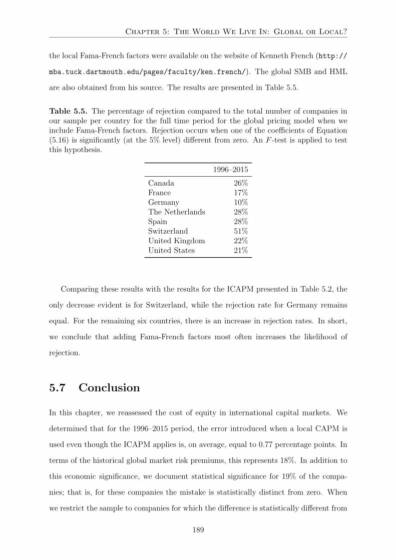
Chapter 5: The World We Live In: Global or Local?
the local Fama-French factors were available on the website of Kenneth French (http://
mba.tuck.dartmouth.edu/pages/faculty/ken.french/). The global SMB and HML
are also obtained from his source. The results are presented in Table 5.5.
Table 5.5. The percentage of rejection compared to the total number of companies inour sample per country for the full time period for the global pricing model when weinclude Fama-French factors. Rejection occurs when one of the coefficients of Equation(5.16) is significantly (at the 5% level) different from zero. An F -test is applied to testthis hypothesis.
1996–2015
Canada 26%France 17%Germany 10%The Netherlands 28%Spain 28%Switzerland 51%United Kingdom 22%United States 21%
Comparing these results with the results for the ICAPM presented in Table 5.2, the
only decrease evident is for Switzerland, while the rejection rate for Germany remains
equal. For the remaining six countries, there is an increase in rejection rates. In short,
we conclude that adding Fama-French factors most often increases the likelihood of
rejection.
5.7 Conclusion
In this chapter, we reassessed the cost of equity in international capital markets. We
determined that for the 1996–2015 period, the error introduced when a local CAPM is
used even though the ICAPM applies is, on average, equal to 0.77 percentage points. In
terms of the historical global market risk premiums, this represents 18%. In addition to
this economic significance, we document statistical significance for 19% of the compa-
nies; that is, for these companies the mistake is statistically distinct from zero. When
we restrict the sample to companies for which the difference is statistically different from
189

Drivers of Bank Performance and The International Cost of Equity
zero, the error jumps to 1.49 percentage points, thereby representing 35% of the histor-
ical risk premium. Therefore, applying the local CAPM instead of the ICAPM can lead
to considerable mistakes in the cost of equity.
We discussed two implications of wrongly estimating the cost of equity: the valua-
tion of the company and the decision to invest. Firstly, overestimation of the cost of
equity implies that the rate by which dividends are discounted to arrive at the stock
price will be too high. The company will thus be undervalued. The opposite holds
true for an underestimation of the cost of equity. Secondly, underestimation might lead
a company to overinvest, since it wrongly believes that projects are profitable enough
when in reality they are not. Again, conversely, overestimation leads to underinvestment.
Among the countries we consider, China presents a special case. The difference in
the cost of equity between the two models is significant for only 1.9% of the Chinese
companies in the full sample. We ascribe this to a lack of integration on the part of the
small Chinese companies we consider. The results for the other BRICs are more in line
with those of the developed countries.
When we extended the model with Fama-French factors, the rejection rates increased
slightly for the majority of the countries. We therefore conclude that our results are
robust for this more general specification.
190

Chapter 5: The World We Live In: Global or Local?
Appendix
A. Methodology
A.1 CAPM Regressions
Start from the global CAPM (ICAPM) in excess returns:
E [Ri] = αG,i + βG,iE [RG] , (A.1)
βG,i =Cov [Ri, RG]
V ar [RG],
αG,i = 0. (A.2)
Let realised returns be
Ri = E [Ri] + ui, (A.3)
RG = E [RG] + uG, (A.4)
with ui and uG be truly unpredictable innovations. Note that this implies that we can
also write
βG,i =Cov [ui, uG]
V ar [uG].
Now consider the regression
Ri = αG,i + βG,iRG + εG,i. (A.5)
Inserting (A.3) and (A.4) into (A.5), and using (A.1) and (A.2), it then follows, after
rearranging, that
εG,i = ui − βG,iuG, (A.6)
191

Drivers of Bank Performance and The International Cost of Equity
which we use to show the validity of the OLS-estimator for Equation (5.2):
Cov [εG,i, RG] = Cov [ui − βG,iuG, uG]
= Cov [ui, uG]− βG,iCov [uG, uG]
= Cov [ui, uG]− Cov [ui, uG]
V ar [uG]V ar [uG]
= 0.
Note that if the ICAPM does not hold, this implies that alpha is not equal to zero. The
model still assumes that beta is driving the expected returns, so we still have that the
residual is orthogonal to the regressor in Equation (A.5).
A.2 Global Versus Local CAPM
The ICAPM also implies for country L:
E [RL] = αG,L + βG,LE [RG] , (A.7)
with the same implications for the regression as above, and αG,L = 0.
The local CAPM on the other hand implies:
E [Ri] = αL,i + βL,iE [RL] , (A.8)
also with the same implications for the accompanying regression, and αL,i = 0.
Similar to above, note that if either the ICAPM or the local CAPM does not hold,
this implies that the alphas are not equal to zero. The models still assume that betas
are driving the expected returns, so we still have that in each regression the residual is
orthogonal to the regressor [in the regressions from Equations (A.7) and (A.8)].
Next, consider a regression of Ri on RL and RG, assuming the ICAPM is valid (i.e.,
192

References
Equations (A.1) and (A.7) hold):
Ri = αi + γL,iRL + γG,iRG + ηi. (A.9)
Using R = E [R] + u, we have that
ηi = ui − γL,iuL − γG,iuG, (A.10)
which is similar to Equation (A.6). To simplify, denote
y = Ri, α = αi, η = ηi, e = ui,
γ′ =
(γL,i γG,i
),
x′ =
(RL RG
),
u′ =
(uL uG
).
So, Equations (A.9) and (A.10) can be written as
y = α + γ′x+ η,
η = e− γ′u.
To check for orthogonality between the residual and the regressors in Equation (5.8):
Cov
ηi, RL
RG
= Cov [η, x] = Cov [e− γ′u, u] = Σeu − γ′Σuu
= Σeu − ΣeuΣ−1uuΣuu = Σeu − Σeu = 0.
193

Drivers of Bank Performance and The International Cost of Equity
B.
Data
Sou
rces
Tab
leB
.1.
Data
typ
esan
ddata
sources
per
country.
Colu
mn
2lists
the
indices
fromw
hich
the
constitu
ents
from1980
to2015
were
selectedas
the
stock
sin
our
sample.
Sto
ckprices
arefrom
Datastream
.E
xch
ange
rates(C
olum
n4)
areeith
erfrom
FR
ED
orD
atastream.
The
correspon
din
gD
atastreamco
de
islisted
inC
olum
n5.
Local
market
indices
areth
enation
alM
SC
Im
arketin
dices,
and
the
global
index
isth
eW
orldM
SC
Iin
dex
.T
he
prices
forall
MSC
Iin
dices
were
obtain
edfrom
Datastream
.
Cou
ntry
Sto
ckp
ricesE
xch
an
ge
Rate
Loca
lM
arketIn
dex
Glob
alM
arketIn
dex
Ind
exS
ou
rceS
ou
rceD
ata
stream
Cod
eIn
dex
Datastream
Cod
eIn
dex
Datastream
Cod
e
Au
straliaA
SX
Datastream
MSCI
MS
AU
ST
L
WorldMSCI
TOTMKWD
Can
ad
aT
SX
MS
CN
DA
LF
ran
ceS
BF
120
MS
FR
NC
LG
erman
yC
DA
XM
SG
ER
ML
Jap
an
NIK
KE
I225
MS
JP
AN
LN
etherla
nd
sA
EX
MSN
ET
HL
Sp
ainIB
EX
35
MS
SP
AN
LS
ou
thK
oreaK
OS
PI
200M
SK
OR
EL
Sw
itzerland
SIP
MS
SW
ITL
U.K
.F
TS
EA
llM
SU
TD
KL
U.S
.S
&P
500
MS
US
AM
L
Brazil
BO
VE
SP
AM
SB
RA
ZL
Ru
ssiaR
TS
Data
stream
CIS
RU
B$
MS
RU
SS
LIn
dia
CN
XN
IFT
YM
SIN
DIL
Ch
ina
SS
EC
omp
ositeF
RE
DM
SC
HIN
L
194

References
Acharya, V. V., Engle, R., & Pierret, D. (2014). Testing macroprudential stress tests:
The risk of regulatory risk weights. Journal of Monetary Economics , 65 , 36–53.
Acharya, V. V., Engle, R., & Richardson, M. (2012). Capital shortfall: A new approach
to ranking and regulating systemic risks. The American Economic Review , 102 (3),
59–64.
Acharya, V. V., Pagano, M., & Volpin, P. (2016). Seeking alpha: Excess risk taking
and competition for managerial talent. The Review of Financial Studies , 29 (10),
2565–2599.
Acharya, V. V., Pedersen, L. H., Philippon, T., & Richardson, M. (2017). Measuring
systemic risk. The Review of Financial Studies , 30 (1), 2–47.
Acharya, V. V., Richardson, M., Van Nieuwerburgh, S., & White, L. J. (2011). Guar-
anteed to Fail: Fannie Mae, Freddie Mac, and the Debacle of Mortgage Finance.
Princeton, NJ: Princeton University Press.
Acharya, V. V., & Schnabl, P. (2009). How banks played the leverage “game”. Financial
Markets, Institutions & Instruments , 18 (2), 144–145.
Acharya, V. V., Schnabl, P., & Suarez, G. (2013). Securitization without risk transfer.
Journal of Financial Economics , 107 (3), 515–536.
Admati, A. R., & Hellwig, M. F. (2013). The Bankers’ New Clothes: What’s Wrong with
Banking and What to Do About It. Princeton, NJ: Princeton University Press.
Adrian, T., & Shin, H. S. (2009). Money, liquidity, and monetary policy. American
Economic Review , 99 (2), 600–605.
Aebi, V., Sabato, G., & Schmid, M. (2012). Risk management, corporate governance, and
195

Drivers of Bank Performance and The International Cost of Equity
bank performance in the financial crisis. Journal of Banking & Finance, 36 (12),
3213–3226.
Agarwal, S., Amromin, G., Ben-David, I., Chomsisengphet, S., & Evanoff, D. D. (2014).
Predatory lending and the subprime crisis. Journal of Financial Economics ,
113 (1), 29–52.
Altunbas, Y., Manganelli, S., & Marques-Ibanez, D. (2011). Bank risk during the
financial crisis: Do business models matter? (ECB Working Paper No. 1394).
Retrieved from European Central Bank website: https://www.ecb.europa.eu/
pub/pdf/scpwps/ecbwp1394.pdf.
Altunbas, Y., & Molyneux, P. (1996). Economies of scale and scope in European banking.
Applied Financial Economics , 6 (4), 367–375.
Angrist, J. D., & Pischke, J.-S. (2009). Mostly Harmless Econometrics: An Empiricist’s
Companion. Princeton, NJ: Princeton University Press.
Ayadi, R., Llewellyn, D., Arbak, E., & de Groen, W. (2010). Investigating Diversity
in the Banking Sector in Europe: Key Developments, Performance, and Role of
Cooperative Banks. Brussels, Belgium: Centre for European Policy Studies.
Baily, M. N., & Elliott, D. J. (2014). How is the system safer? What more is needed?
In M. N. Baily & J. B. Taylor (Eds.), Across the Great Divide: New Perspectives
on the Financial Crisis (pp. 165–195). Stanford, CA: Hoover Institution Press.
Bank of England and European Central Bank. (2014). The case for a better functioning
securitisation market in the European Union (Discussion Paper). Retrieved from
European Central Bank website: https://www.ecb.europa.eu/pub/pdf/other/
ecb-boe case better functioning securitisation marketen.pdf.
Barth, J. R., Caprio, G., & Levine, R. (2012). Guardians of Finance: Making Regulators
Work for Us. Cambridge, MA: MIT Press.
Barth, J. R., Nolle, D. E., Phumiwasana, T., & Yago, G. (2003). A cross-country
analysis of the bank supervisory framework and bank performance. Financial
Markets, Institutions & Instruments , 12 (2), 67–120.
Bayazitova, D., & Shivdasani, A. (2011). Assessing TARP. The Review of Financial
196

References
Studies , 25 (2), 377–407.
Bebchuk, L. A., & Fried, J. (2004). Pay Without Performance: The Unfulfilled Promise
of Executive Compensation. Cambridge, MA: Harvard University Press.
Bekaert, G., & Harvey, C. R. (2003). Emerging markets finance. Journal of Empirical
Finance, 10 (1), 3–55.
Bekaert, G., Harvey, C. R., Lundblad, C. T., & Siegel, S. (2011). What segments equity
markets? The Review of Financial Studies , 24 (12), 3841–3890.
Bekaert, G., & Hodrick, R. J. (2009). International Financial Management. New Jersey,
NJ: Pearson Prentice Hall.
Beltratti, A., & Stulz, R. M. (2012). The credit crisis around the globe: Why did some
banks perform better? Journal of Financial Economics , 105 (1), 1–17.
Bennedsen, M., Perez-Gonzalez, F., & Wolfenzon, D. (2006). Do CEOs matter? (NYU
Working Paper No. FIN-06-032). Retrieved from SSRN website: https://ssrn
.com/abstract=1293659.
Berger, A. N. (1995a). The profit-structure relationship in banking–tests of market-
power and efficient-structure hypotheses. Journal of Money, Credit and Banking ,
27 (2), 404–431.
Berger, A. N. (1995b). The relationship between capital and earnings in banking. Journal
of Money, Credit and Banking , 27 (2), 432–456.
Berger, A. N., & Bouwman, C. H. (2013). How does capital affect bank performance
during financial crises? Journal of Financial Economics , 109 (1), 146–176.
Berger, A. N., & DeYoung, R. (1997). Problem loans and cost efficiency in commercial
banks. Journal of Banking & Finance, 21 (6), 849–870.
Berger, A. N., Hanweck, G. A., & Humphrey, D. B. (1987). Competitive viability in
banking. Journal of Monetary Economics , 20 (3), 501–520.
Berger, A. N., Herring, R. J., & Szego, G. P. (1995). The role of capital in financial
institutions. Journal of Banking & Finance, 19 (3), 393–430.
Bertrand, M., & Schoar, A. (2003). Managing with style: The effect of managers on
firm policies. Quarterly Journal of Economics , 118 (4), 1169–1208.
197
Drivers of Bank Performance and The International Cost of Equity
Bhagat, S., & Bolton, B. (2014). Financial crisis and bank executive incentive compen-
sation. Journal of Corporate Finance, 25 , 313–341.
Board of Governors of the Federal Reserve System. (2009). The supervisory capital
assessment program: Overview of results. Retrieved from www.federalreserve
.gov.
Bornemann, S., Kick, T., Pfingsten, A., & Schertler, A. (2015). Earnings baths by
CEOs during turnovers: Empirical evidence from German savings banks. Journal
of Banking & Finance, 53 , 188–201.
Bowden, M. P., & Doughney, J. (2010). Socio-economic status, cultural diversity and the
aspirations of secondary students in the Western Suburbs of Melbourne, Australia.
Higher Education, 59 (1), 115–129.
Breen, R., & Goldthorpe, J. H. (1999). Class inequality and meritocracy: A critique
of Saunders and an alternative analysis. The British Journal of Sociology , 50 (1),
1–27.
Brounen, D., De Jong, A., & Koedijk, K. (2004). Corporate finance in Europe: Con-
fronting theory with practice. Financial Management , 33 (4), 71–101.
Brownlees, C., & Engle, R. F. (2017). Srisk: A conditional capital shortfall measure of
systemic risk. The Review of Financial Studies , 30 (1), 48–79.
Brunnermeier, M. K. (2009). Deciphering the liquidity and credit crunch 2007-2008.
Journal of Economic Perspectives , 23 (1), 77–100.
Calomiris, C. W. (2009). The subprime turmoil: What’s old, what’s new, and what’s
next. The Journal of Structured Finance, 15 (1), 6–52.
Calomiris, C. W., Eisenbeis, R. A., & Litan, R. E. (2012). Financial crisis in the US
and beyond. In R. E. Litan (Ed.), The World in Crisis: Insights from Six Shadow
Financial Regulatory Committees from Around the World (pp. 1–60). Philadelphia,
PA: Wharton Financial Institutions Center.
Calomiris, C. W., & Haber, S. H. (2014). Fragile by Design: The Political Origins of
Banking Crises and Scarce Credit. Princeton, NJ: Princeton University Press.
Calomiris, C. W., & Herring, R. J. (2013). How to design a contingent convertible
198

References
debt requirement that helps solve our too-big-to-fail problem. Journal of Applied
Corporate Finance, 25 (2), 39–62.
Calomiris, C. W., & Khan, U. (2015). An assessment of TARP assistance to financial
institutions. The Journal of Economic Perspectives , 29 (2), 53–80.
Cameron, A. C., & Trivedi, P. K. (2009). Microeconometrics Using Stata (Rev. ed.).
College Station, TX: Stata Press.
Carrieri, F., Chaieb, I., & Errunza, V. (2013). Do implicit barriers matter for globaliza-
tion? The Review of Financial Studies , 26 (7), 1694–1739.
Cheng, I.-H., Hong, H., & Scheinkman, J. A. (2015). Yesterday’s heroes: Compensation
and risk at financial firms. The Journal of Finance, 70 (2), 839–879.
Claessens, S., DellAriccia, G., Igan, D., & Laeven, L. (2010). Cross-country experiences
and policy implications from the global financial crisis. Economic Policy , 25 (62),
267–293.
Claessens, S., Djankov, S., & Xu, L. C. (2000). Corporate performance in the East Asian
financial crisis. The World Bank Research Observer , 15 (1), 23–46.
Cole, R. A., & White, L. J. (2012). Deja vu all over again: The causes of US commercial
bank failures this time around. Journal of Financial Services Research, 42 (1),
5–29.
Credit Suisse. (2016). Credit Suisse Global Investment Returns Yearbook 2016. Zurich,
Switzerland: Credit Suisse AG.
Delis, M. D., & Kouretas, G. P. (2011). Interest rates and bank risk-taking. Journal of
Banking & Finance, 35 (4), 840–855.
Demirguc-Kunt, A., Detragiache, E., & Gupta, P. (2006). Inside the crisis: An empir-
ical analysis of banking systems in distress. Journal of International Money and
Finance, 25 (5), 702–718.
Demirguc-Kunt, A., Detragiache, E., & Merrouche, O. (2013). Bank capital: Lessons
from the financial crisis. Journal of Money, Credit and Banking , 45 (6), 1147–1164.
Demirguc-Kunt, A., & Huizinga, H. (1999). Determinants of commercial bank interest
margins and profitability: Some international evidence. World Bank Economic
199

Drivers of Bank Performance and The International Cost of Equity
Review , 13 (2), 379–408.
Demirguc-Kunt, A., & Huizinga, H. (2001). Financial structure and bank profitability. In
A. Demirguc-Kunt & R. Levine (Eds.), Financial Structure and Economic Growth:
A Cross-country Comparison of Banks, Markets, and Development (pp. 243–261).
Boston, MA: MIT press.
Demirguc-Kunt, A., & Huizinga, H. (2010). Bank activity and funding strategies: The
impact on risk and returns. Journal of Financial Economics , 98 (3), 626–650.
Diamond, D. W., & Rajan, R. G. (2009). The credit crisis: Conjectures about causes
and remedies. American Economic Review , 99 (2), 606–610.
Dimson, E., Marsh, P., & Staunton, M. (2009). Triumph of the Optimists: 101 Years of
Global Investment Returns. Princeton, NJ: Princeton University Press.
Doidge, C., Karolyi, G. A., & Stulz, R. M. (2017). The U.S. listing gap. Journal of
Financial Economics , 123 (3), 464–487.
Dumas, B., & Solnik, B. (1995). The world price of foreign exchange risk. The Journal
of Finance, 50 (2), 445–479.
Duncan, G. J., Ziol-Guest, K. M., & Kalil, A. (2010, 2). Early-childhood poverty and
adult attainment, behavior, and health. Child Development , 81 (1), 306–325.
Edwards, F. R., & Heggestad, A. A. (1973). Uncertainty, market structure, and perfor-
mance: The Galbraith-Caves hypothesis and managerial motives in banking. The
Quarterly Journal of Economics , 87 (3), 455–473.
The Economist. (2007, September 20). When it goes wrong... The Economist .
The Economist. (2017a, May 6). Sheep and goats. The Economist .
The Economist. (2017b, May 6). Ten years on. The Economist .
Ellul, A., & Yerramilli, V. (2013). Stronger risk controls, lower risk: Evidence from US
bank holding companies. The Journal of Finance, 68 (5), 1757–1803.
Erikson, R., & Goldthorpe, J. H. (2002). Intergenerational inequality: A sociological
perspective. Journal of Economic Perspectives , 16 (3), 31–44.
Erkens, D. H., Hung, M., & Matos, P. (2012). Corporate governance in the 2007–
2008 financial crisis: Evidence from financial institutions worldwide. Journal of
200

References
Corporate Finance, 18 (2), 389–411.
Errunza, V., & Losq, E. (1985). International asset pricing under mild segmentation:
Theory and test. The Journal of Finance, 40 (1), 105–124.
Fahlenbrach, R., Prilmeier, R., & Stulz, R. M. (2012). This time is the same: Using
bank performance in 1998 to explain bank performance during the recent financial
crisis. The Journal of Finance, 67 (6), 2139–2185.
Fahlenbrach, R., Prilmeier, R., & Stulz, R. M. (2016). Why does fast loan growth predict
poor performance for banks? (NBER Working Paper No. 22089). Retrieved from
National Bureau of Economic Research website: http://www.nber.org/papers/
w22089.
Fahlenbrach, R., & Stulz, R. M. (2011). Bank CEO incentives and the credit crisis.
Journal of Financial Economics , 99 (1), 11–26.
Fama, E. F., & French, K. R. (1993). Common risk factors in the returns on stocks and
bonds. Journal of Financial Economics , 33 (1), 3–56.
Financial Stability Board. (2015). Implementation and effects of the G20 financial reg-
ulatory reforms. Retrieved from http://www.fsb.org/2015/11/implementation
-and-effects-of-the-g20-financial-regulatory-reforms/.
Fisher, I. (1896). What is capital? The Economic Journal , 6 (24), 509–534.
Fisher, R. A. (1935). The logic of inductive inference. Journal of the Royal Statistical
Society , 98 (1), 39–82.
Frisch, R., & Waugh, F. V. (1933). Partial time regressions as compared with individual
trends. Econometrica, 1 (4), 387–401.
Gabaix, X., & Landier, A. (2008). Why has CEO pay increased so much? The Quarterly
Journal of Economics , 123 (1), 49–100.
Giddens, A. (1979). Central Problems in Social Theory: Action, Structure, and Con-
tradiction in Social Analysis. London and Basingstoke, England: The Macmillan
Press.
Gompers, P., Ishii, J., & Metrick, A. (2003). Corporate governance and equity prices.
The Quarterly Journal of Economics , 118 (1), 107–156.
201

Drivers of Bank Performance and The International Cost of Equity
Gordon, M. J. (1962). The Investment, Financing, and Valuation of the Corporation.
Berkeley, CA: University of California Press.
Gordon, M. J., & Shapiro, E. (1956). Capital equipment analysis: The required rate of
profit. Management Science, 3 (1), 102–110.
Gorton, G., & Metrick, A. (2012). Getting up to speed on the financial crisis: A
one-weekend-reader’s guide. Journal of Economic Literature, 50 (1), 128–50.
Graham, J. R., & Harvey, C. R. (2001). The theory and practice of corporate finance:
Evidence from the field. Journal of Financial Economics , 60 (2), 187–243.
Graham, J. R., Harvey, C. R., & Puri, M. (2013). Managerial attitudes and corporate
actions. Journal of Financial Economics , 109 (1), 103–121.
Grauer, F. L., Litzenberger, R. H., & Stehle, R. E. (1976). Sharing rules and equilib-
rium in an international capital market under uncertainty. Journal of Financial
Economics , 3 (3), 233–256.
Griffin, J. M., & Stulz, R. M. (2001). International competition and exchange rate
shocks: A cross-country industry analysis of stock returns. The Review of Financial
Studies , 14 (1), 215–241.
Griffin, J. M., & Tang, D. Y. (2012). Did subjectivity play a role in CDO credit ratings?
The Journal of Finance, 67 (4), 1293–1328.
Hambrick, D. C., & Mason, P. A. (1984). Upper echelons: The organization as a
reflection of its top managers. Academy of Management Review , 9 (2), 193–206.
Harris, R. S., Marston, F. C., Mishra, D. R., & O’Brien, T. J. (2003). Ex ante cost
of equity estimates of S&P 500 firms: The choice between global and domestic
CAPM. Financial Management , 32 (3), 51–66.
Hayashi, F. (2000). Econometrics. Princeton, NJ: Princeton University.
Ho, P.-H., Huang, C.-W., Lin, C.-Y., & Yen, J.-F. (2016). CEO overconfidence and
financial crisis: Evidence from bank lending and leverage. Journal of Financial
Economics , 120 (1), 194–209.
Hoque, H. (2013). From the credit crisis to the sovereign debt crisis: Determinants
of share price performance of global banks. International Review of Financial
202

References
Analysis , 30 , 334–350.
Hoque, H., Andriosopoulos, D., Andriosopoulos, K., & Douady, R. (2015). Bank regula-
tion, risk and return: Evidence from the credit and sovereign debt crises. Journal
of Banking & Finance, 50 , 455–474.
Huber, P. J. (1964). Robust estimation of a location parameter. The Annals of Mathe-
matical Statistics , 35 (1), 73–101.
Huber, P. J., & Ronchetti, E. M. (2009). Robust Statistics. Hoboken, NJ: Wiley.
Iannotta, G., Nocera, G., & Sironi, A. (2007). Ownership structure, risk and performance
in the European banking industry. Journal of Banking & Finance, 31 (7), 2127–
2149.
Jacquillat, B., & Solnik, B. (1978). Multinationals are poor tools for diversification. The
Journal of Portfolio Management , 4 (2), 8–12.
Jenter, D., & Kanaan, F. (2015). CEO turnover and relative performance evaluation.
The Journal of Finance, 70 (5), 2155–2184.
Jenter, D., & Lewellen, K. (2010). Performance-induced CEO turnover (Stanford Uni-
versity Graduate School of Business Working Paper 3054). Retrieved from SSRN
website: https://ssrn.com/abstract=1570635.
Jenter, D., Matveyev, E., & Roth, L. (2016). Good and bad CEOs (Working Paper).
Kaminsky, G. L., & Reinhart, C. M. (1999). The twin crises: The causes of banking and
balance-of-payments problems. The American Economic Review , 89 (3), 473–500.
Karolyi, G. A., & Stulz, R. M. (2003). Are financial assets priced locally or globally? In
G. M. Constantinides, M. Harris, & R. M. Stulz (Eds.), Handbook of the Economics
of Finance (Vol. 1B, pp. 975–1020). Amsterdam, Netherlands: Elsevier.
Kedia, S., & Philippon, T. (2009). The economics of fraudulent accounting. The Review
of Financial Studies , 22 (6), 2169–2199.
Kelly, B. T., Lustig, H., & Van Nieuwerburgh, S. (2011). Too-systemic-to-fail: What
option markets imply about sector-wide government guarantees (NBER Working
Paper No. 17149). Retrieved from National Bureau of Economic Research website:
http://www.nber.org/papers/w17149.
203
Drivers of Bank Performance and The International Cost of Equity
Keoun, B. (2014, August 22). Fed’s $1.2 trillion loan lifelines dwarfed TARP: Glossary.
Bloomberg . Retrieved from www.bloomberg.com.
Keys, B. J., Mukherjee, T., Seru, A., & Vig, V. (2010). Did securitization lead to lax
screening? Evidence from subprime loans. The Quarterly Journal of Economics ,
125 (1), 307–362.
Kiel, P., & Nguyen, D. (2015). Bailout tracker. ProPublica. Retrieved from www
.propublica.org.
Kirkpatrick, G. (2009). The corporate governance lessons from the financial crisis.
Financial Market Trends , 1 (96), 1–30.
Kish-Gephart, J., & Campbell, J. T. (2015). You don’t forget your roots: The influence
of CEO social class background on strategic risk taking. Academy of Management
Journal , 58 (6), 1614–1636.
Kleibergen, F., & Paap, R. (2006). Generalized reduced rank tests using the singular
value decomposition. Journal of Econometrics , 133 (1), 97–126.
Kleibergen, F., & Schaffer, M. E. (2007). Ranktest: Stata module to test the rank of a
matrix using the Kleibergen-Paap rk statistic. Statistical Software Components .
Koedijk, K. G., Kool, C. J., Schotman, P. C., & Van Dijk, M. A. (2002). The cost of
capital in international financial markets: Local or global? Journal of International
Money and Finance, 21 (6), 905–929.
Kok, C., More, C., & Pancaro, C. (2015). Bank profitability challenges in euro area
banks: The role of cyclical and structural factors. Financial Stability Review,
European Central Bank , 148–159.
Krause, R., Semadeni, M., & Cannella, A. A. (2014). CEO duality. Journal of Manage-
ment , 40 (1), 256–286.
Lawson, T. (1994). A realist theory of economics. In R. E. Backhouse (Ed.), New
Directions in Economic Methodology (pp. 257–284). Londen, England: Routledge.
Lo, A. W. (2012). Reading about the financial crisis: A twenty-one-book review. Journal
of Economic Literature, 50 (1), 151–178.
Malmendier, U., & Tate, G. (2005). CEO overconfidence and corporate investment. The
204

References
Journal of Finance, 60 (6), 2661–2700.
Malmendier, U., & Tate, G. (2008). Who makes acquisitions? CEO overconfidence and
the market’s reaction. Journal of Financial Economics , 89 (1), 20–43.
Mann, H. B., & Whitney, D. R. (1947). On a test of whether one of two random variables
is stochastically larger than the other. The Annals of Mathematical Statistics , 50–
60.
Martin, S. R., Cote, S., & Woodruff, T. (2016). Echoes of our upbringing: How growing
up wealthy or poor relates to narcissism, leader behavior, and leader effectiveness.
Academy of Management Journal , 59 (6), 2157–2177.
McAllister, P. H., & McManus, D. (1993). Resolving the scale efficiency puzzle in
banking. Journal of Banking & Finance, 17 (2), 389–405.
Meindl, J. R., Ehrlich, S. B., & Dukerich, J. M. (1985). The romance of leadership.
Administrative Science Quarterly , 30 (1), 78–102.
Molyneux, P., & Forbes, W. (1995). Market structure and performance in European
banking. Applied Economics , 27 (2), 155–159.
Moore, M. L. (1973). Management changes and discretionary accounting decisions.
Journal of Accounting Research, 11 (1), 100–107.
Mullins, W., & Schoar, A. (2016). How do CEOs see their roles? Management philoso-
phies and styles in family and non-family firms. Journal of Financial Economics ,
119 (1), 24–43.
Murphy, K. J. (1999). Executive compensation. In O. C. Ashenfelter & D. Card (Eds.),
Handbook of Labor Economics (Vol. 3B, pp. 2485–2563). Amsterdam, Netherlands:
Elsevier.
Nakamoto, M., & Wighton, D. (2007, July 9). Citigroup chief stays bullish on buyouts.
Financial Times . Retrieved from http://www.ft.com/cms/s/0/80e2987a-2e50
-11dc-821c-0000779fd2ac.html.
Petersen, M. A. (2009). Estimating standard errors in finance panel data sets: Comparing
approaches. The Review of Financial Studies , 22 (1), 435–480.
Piskorski, T., Seru, A., & Witkin, J. (2015). Asset quality misrepresentation by financial
205

Drivers of Bank Performance and The International Cost of Equity
intermediaries: Evidence from the RMBS market. The Journal of Finance, 70 (6),
2635–2678.
Pourciau, S. (1993). Earnings management and nonroutine executive changes. Journal
of Accounting and Economics , 16 (1), 317–336.
Pozsar, Z., Adrian, T., Ashcraft, A. B., & Boesky, H. (2010). Shadow banking (Fed-
eral Reserve Bank of New York Staff Report No. 458). Retrieved from Federal
Reserve Bank of New York website: https://www.newyorkfed.org/research/
staff reports/sr458.html.
Rajan, R. G. (1994). Why bank credit policies fluctuate: A theory and some evidence.
The Quarterly Journal of Economics , 109 (2), 399–441.
Rajan, R. G. (2006). Has finance made the world riskier? European Financial Manage-
ment , 12 (4), 499–533.
Reed, M. (2005). Reflections on the ‘realist turn’ in organization and management
studies. Journal of Management Studies , 42 (8), 1621–1644.
Reinhart, C. M., & Rogoff, K. S. (2011). From financial crash to debt crisis. The
American Economic Review , 101 (5), 1676–1706.
Roll, R. (1986). The hubris hypothesis of corporate takeovers. The Journal of Business ,
59 (2), 197–216.
Romero, C. L. (2011). Exiting TARP: Repayments by the largest financial institutions.
Retrieved from www.sigtarp.gov.
Rousseeuw, P. J., & Leroy, A. M. (2003). Robust Regression and Outlier Detection. New
York, NY: John Wiley & Sons.
Rousseeuw, P. J., & Yohai, V. J. (1984). Robust regression by means of S-estimators.
In J. Franke, W. Hardle, & D. Martin (Eds.), Robust and Nonlinear Time Series
Analysis (pp. 256–272). New York, NY: Springer.
Scott, W. R. (2008). Institutions and Organizations: Ideas and Interests (3rd ed.).
Thousand Oaks, CA: Sage Publications.
Sercu, P. (1980). A generalization of the international asset pricing model. Revue de
l’Association Francaise de Finance, 1 (1), 91–135.
206

References
Shleifer, A., & Vishny, R. W. (1997). A survey of corporate governance. The Journal of
Finance, 52 (2), 737–783.
Shleifer, A., & Vishny, R. W. (2010). Unstable banking. Journal of Financial Economics ,
97 (3), 306–318.
Solnik, B. H. (1974a). An equilibrium model of the international capital market. Journal
of Economic Theory , 8 (4), 500–524.
Solnik, B. H. (1974b). The international pricing of risk: An empirical investigation of
the world capital market structure. The Journal of Finance, 29 (2), 365–378.
Solon, G. (2002). Cross-country differences in intergenerational earnings mobility. Jour-
nal of Economic Perspectives , 16 (3), 59–66.
Stein, M. (2007). Oedipus rex at enron: Leadership, Oedipal struggles, and organiza-
tional collapse. Human Relations , 60 (9), 1387–1410.
Stiglitz, J. E. (2009, January). Capitalist fools. Vanity Fair . Retrieved from http://
www.vanityfair.com/news/2009/01/stiglitz200901.
Strong, J. S., & Meyer, J. R. (1987). Asset writedowns: Managerial incentives and
security returns. The Journal of Finance, 42 (3), 643–661.
Stulz, R. M. (1995). The cost of capital in internationally integrated markets: The case
of Nestle. European Financial Management , 1 (1), 11–22.
Stulz, R. M. (2005). The limits of financial globalization. The Journal of Finance,
60 (4), 1595–1638.
Tervio, M. (2008). The difference that CEOs make: An assignment model approach.
The American Economic Review , 98 (3), 642–668.
Tuckett, D. (2011). Minding the Markets: An Emotional Finance View of Financial
Instability. Basingstoke, England: Palgrave Macmillan.
Verardi, V., & Croux, C. (2009). Robust regression in Stata. Stata Journal , 9 (3),
439–453.
Welch, B. L. (1947). The generalization of ‘student’s’ problem when several different
population variances are involved. Biometrika, 34 (1–2), 28–35.
Wilcoxon, F. (1945). Individual comparisons by ranking methods. Biometrics Bulletin,
207
Drivers of Bank Performance and The International Cost of Equity
1 (6), 80–83.
Williams, J. B. (1938). The Theory of Investment Value. Cambridge, MA: Harvard
University Press.
Wolf, M. (2014, May 27). Disarm our doomsday machine. Financial Times . Retrieved
from www.ft.com.
Yang, T., & Zhao, S. (2014). CEO duality and firm performance: Evidence from an
exogenous shock to the competitive environment. Journal of Banking & Finance,
49 , 534–552.
Yohai, V. J. (1987). High breakdown-point and high efficiency robust estimates for
regression. The Annals of Statistics , 15 (2), 642–656.
Zingales, L. (2015a). The “cultural revolution” in finance. Journal of Financial Eco-
nomics , 117 (1), 1–4.
Zingales, L. (2015b). Does finance benefit society? The Journal of Finance, 70 (4),
1327–1363.
208