Essays on Finance and Macroeconomics

Cynthia Mei Balloch

Submitted in partial fulfillment of therequirements for the degree of

Doctor of Philosophyin the Graduate School of Arts and Sciences

COLUMBIA UNIVERSITY

2018

c© 2018Cynthia Mei BallochAll rights reserved

ABSTRACT

Essays on Finance and Macroeconomics

Cynthia Mei Balloch

My dissertation studies the impact of banks on macroeconomic outcomes. Chapter

1 explores the effects of bond market growth on the financing decisions of firms, the

lending behavior of banks, and the resulting equilibrium allocation of credit and capi-

tal. This chapter makes three contributions to understand the impact of bond market

liberalization. First, using evidence from reforms in Japan that gave borrowers selective

access to bond markets during the 1980s, it shows that firms that obtained access to

the bond market used bond issuance to pay back bank debt. More importantly, this

large, positive funding shock led banks to increase lending to small and medium enter-

prises and real estate firms. Second, it proposes a model of financial frictions that is

consistent with the empirical findings, and uses the model to derive general conditions

under which bond liberalization has this effect on banks. The model predicts that bond

liberalization can significantly worsen the quality of the pool of bank borrowers, and so

lower bank profitability. These results suggest that Japan’s bond market liberalization

contributed to both the real estate bubble in the 1980s and bank problems in the 1990s.

Third, the model implies that bond markets amplify the effects of shocks to the risk-free

rate and firm borrowing, in addition to attenuating the effects of financial shocks.

In Chapter 2, I explore how the incentives of domestic banks and sovereign govern-

ments interact. I build a model of government default and banks that invest in the debt

of their own sovereign. In the model, banks demand safe assets to use as collateral,

and default affects bank equity. These losses inhibit banks’ ability to attract deposits,

leading to lower private credit provision, and lower output. This disincentivizes the

sovereign from defaulting. The extent of output losses depends on characteristics of

the banking system, including sovereign exposures, equity, and deposits. In turn, bank

exposures are affected by default risk. The model is also used to show that policies

such as financial repression can improve welfare, but worsen output losses in the event

of default, and may also worsen losses in some non-default states.

Underlying much research on the role of financial intermediaries in macroeconomics

is an implicit recognition that there is matching between banks and firms, which I turn

to in Chapter 3. Matching between banks and firms has implications for both the

transmission of macroeconomic shocks and for empirical estimates of the effects of such

shocks. This paper presents a theory of matching in corporate loan markets, between

heterogeneous banks and heterogenous firms. The model demonstrates how assortative

matching can cause shocks to have distributional consequences, where particular types

of banks and firms are disproportionately affected. The framework is used to show (1)

why growth without financial development is limited, (2) how capital inflows affect bank

and firm outcomes, and (3) how financial regulation for certain banks also has implica-

tions for other borrowers and lenders. Further, this theory demonstrates that matching

in corporate lending markets is analytically tractable, and generates predictions that

are consistent with existing empirical evidence.

Contents

List of Figures iii

List of Tables v

1 Inflows and spillovers: Tracing the impact of bond market liberal-

ization 1

1.1 Introduction . . . . . . . . . . . . . . . . . . . . . . . . . . . . . . . . . 2

1.2 Institutional background and data . . . . . . . . . . . . . . . . . . . . . 13

1.3 Empirical evidence . . . . . . . . . . . . . . . . . . . . . . . . . . . . . 17

1.4 Model . . . . . . . . . . . . . . . . . . . . . . . . . . . . . . . . . . . . 31

1.5 Implications . . . . . . . . . . . . . . . . . . . . . . . . . . . . . . . . . 46

1.6 Conclusion . . . . . . . . . . . . . . . . . . . . . . . . . . . . . . . . . . 56

2 Default, commitment, and domestic bank holdings of sovereign debt 58

2.1 Introduction . . . . . . . . . . . . . . . . . . . . . . . . . . . . . . . . . 58

2.2 Model . . . . . . . . . . . . . . . . . . . . . . . . . . . . . . . . . . . . 64

2.3 Results . . . . . . . . . . . . . . . . . . . . . . . . . . . . . . . . . . . . 74

2.4 Externalities and financial repression . . . . . . . . . . . . . . . . . . . 86

2.5 Extensions . . . . . . . . . . . . . . . . . . . . . . . . . . . . . . . . . . 90

2.6 Conclusion . . . . . . . . . . . . . . . . . . . . . . . . . . . . . . . . . . 93

3 Matching in corporate loan markets and macroeconomic shocks 95

3.1 Introduction . . . . . . . . . . . . . . . . . . . . . . . . . . . . . . . . . 96

i

3.2 Model . . . . . . . . . . . . . . . . . . . . . . . . . . . . . . . . . . . . 101

3.3 Applications . . . . . . . . . . . . . . . . . . . . . . . . . . . . . . . . . 113

3.4 Conclusion . . . . . . . . . . . . . . . . . . . . . . . . . . . . . . . . . . 120

Bibliography 122

A Appendix to Chapter 1 129

A.1 Issuance criteria . . . . . . . . . . . . . . . . . . . . . . . . . . . . . . 130

A.2 Additional empirical results . . . . . . . . . . . . . . . . . . . . . . . . 131

A.3 Proofs . . . . . . . . . . . . . . . . . . . . . . . . . . . . . . . . . . . . 134

B Appendix to Chapter 2 138

B.1 Proofs . . . . . . . . . . . . . . . . . . . . . . . . . . . . . . . . . . . . 139

C Appendix to Chapter 3 145

C.1 Proofs . . . . . . . . . . . . . . . . . . . . . . . . . . . . . . . . . . . . 146

C.2 Imperfect competition case . . . . . . . . . . . . . . . . . . . . . . . . . 150

ii

List of Figures

1.1 Debt securities / bank loans of private non-financial corporations (%) . . . 2

1.2 Major policy changes and bonds as a fraction of total debt . . . . . . . . . 14

1.3 Firms qualified to issue unsecured convertible bonds under accounting criteria 15

1.4 Loans as a % of total bank lending . . . . . . . . . . . . . . . . . . . . . . 16

1.5 Bond issuance pre-trends and dynamics . . . . . . . . . . . . . . . . . . . . 23

1.6 Bank debt pre-trends and dynamics . . . . . . . . . . . . . . . . . . . . . . 23

1.7 Comparison between affected and unaffected banks . . . . . . . . . . . . . 33

1.8 Entrepreneurs’ decisions . . . . . . . . . . . . . . . . . . . . . . . . . . . . 39

1.9 Bond market liberalization . . . . . . . . . . . . . . . . . . . . . . . . . . . 42

1.10 Foreign bond issuance and bank deposits . . . . . . . . . . . . . . . . . . . 46

1.11 Decline in the risk free rate . . . . . . . . . . . . . . . . . . . . . . . . . . 49

1.12 Increasing firm borrowing . . . . . . . . . . . . . . . . . . . . . . . . . . . 52

1.13 Bank shocks . . . . . . . . . . . . . . . . . . . . . . . . . . . . . . . . . . . 55

2.1 Heterogeneous bank balance sheets . . . . . . . . . . . . . . . . . . . . . . 68

2.2 For deposits to fall after default, assuming nd1 < N . . . . . . . . . . . . . 73

2.3 Threshold level of A1 . . . . . . . . . . . . . . . . . . . . . . . . . . . . . . 77

2.4 Domestic demand for government debt . . . . . . . . . . . . . . . . . . . . 80

2.5 Domestic share of total debt . . . . . . . . . . . . . . . . . . . . . . . . . . 82

2.6 Bond price and total resources borrowed from abroad . . . . . . . . . . . . 83

2.7 Total resources borrowed . . . . . . . . . . . . . . . . . . . . . . . . . . . . 84

2.8 Effect of increasing domestically held debt . . . . . . . . . . . . . . . . . . 85

iii

2.9 Financial repression can increase welfare . . . . . . . . . . . . . . . . . . . 89

3.1 Share of uninformed capital . . . . . . . . . . . . . . . . . . . . . . . . . . 105

3.2 Investment size . . . . . . . . . . . . . . . . . . . . . . . . . . . . . . . . . 107

3.3 Matching pattern for discrete banks . . . . . . . . . . . . . . . . . . . . . . 111

3.4 Firm distribution, capital distribution, and matching . . . . . . . . . . . . 111

3.5 Firm and bank leverage . . . . . . . . . . . . . . . . . . . . . . . . . . . . 112

3.6 Multiple bank matches . . . . . . . . . . . . . . . . . . . . . . . . . . . . . 112

3.7 Productivity shock . . . . . . . . . . . . . . . . . . . . . . . . . . . . . . . 114

3.8 A fall in γ . . . . . . . . . . . . . . . . . . . . . . . . . . . . . . . . . . . . 116

3.9 Capital inflows to banks . . . . . . . . . . . . . . . . . . . . . . . . . . . . 117

3.10 Shock to large banks . . . . . . . . . . . . . . . . . . . . . . . . . . . . . . 119

iv

List of Tables

1.1 Total debt securities outstanding, non-financial corporations (US$ bn) . . . 3

1.2 The effect of bond market access on bond issuance, 1977-90 . . . . . . . . 21

1.3 The effect of bond issuance on bank borrowing, 1977-90 . . . . . . . . . . . 25

1.4 The effect of bond issuance on bank borrowing, discontinuity sample, 1977-90 25

1.5 Repayment shocks, 1983-87 (%) . . . . . . . . . . . . . . . . . . . . . . . . 29

1.6 Balancing of covariates in the sample, 1983-87 (%) . . . . . . . . . . . . . 30

1.7 The effect of repayment shocks on bank lending, 1983-1987 . . . . . . . . 31

1.8 The effect of repayment shocks on bank lending, 1983-1987 . . . . . . . . . 32

3.1 Available projects . . . . . . . . . . . . . . . . . . . . . . . . . . . . . . . . 102

A.1 Accounting Criteria for Issuance of Domestic Convertible Bonds . . . . . . 130

A.2 Ratings criteria for Issuance of Domestic Convertible Bonds . . . . . . . . 131

A.3 The effect of bond market access on other firm outcomes, 1977-90 . . . . . 132

A.4 The effect of bond market access on other firm outcomes, continued, 1977-90 133

v

Acknowledgements

I would like to thank Emi Nakamura, Ricardo Reis, and Jon Steinsson for their ad-

vice, encouragement, insight, and support over the course of this project. For their

guidance and feedback, I am grateful to Hassan Afrouzi, Patrick Bolton, Olivier Dar-

mouni, Andres Drenik, Martin Guzman, Takatoshi Ito, Jennifer La’O, Jaromir Nosal,

Jesse Schreger, Jose Scheinkman, Stephanie Schmitt-Grohe, Joseph Stiglitz, David We-

instein, and Martin Uribe. The staff at the Columbia Economics department were also

extremely helpful: Shane Bordeau, Amy Devine, Julie Stevens, and Angela Reid, in

particular.

I also thank my colleagues and friends, Tuo Chen, Golvine de Rochambeau, Keshav

Dogra, Sandesh Dhungana, Stephane Dupraz, Juan Herreno, Julian Richers, Pablo

Slutzky, Valentin Somma, and Savitar Sundaresan, for their advice and conversations.

Finally, I thank my family, and especially Juan Navarro-Staicos and Nicolas Navarro-

Balloch, for providing me with support, inspiration, and welcome distractions.

vi

Chapter 1

Inflows and spillovers: Tracing the

impact of bond market

liberalization

1

1.1 Introduction

Bond financing is growing in many markets. The total outstanding debt securities of

US non-financial corporations grew from $3.2 to $5.8 trillion between 2006 and 2016,

and relative to the stock of bank loans has more than doubled since 1990, as shown

in Figure 1.1. Elsewhere in the world, including Europe and especially China, bond

markets have also grown rapidly, as shown in Table 1.1. The shift to bond financing is

partly a product of government support for market-based financing, and partly a result

of borrowers seeking alternative forms of financing in the context of recent banking

crises. This shift raises a number of important questions, of which this chapter focuses

on three. First, how does access to bond markets affect firm borrowing and bank

lending? Second, what are the consequences of growing bond markets for the aggregate

allocation of capital? Third, how do bond markets affect the reaction of an economy

to capital inflows, financial crises, and other shocks?

In this paper, I exploit a natural experiment in Japan to study the consequences of

a transition from bank-centered to market-based financing. Japan liberalized its bond

markets during the 1980s, giving specific types of firms permission to issue bonds and

Figure 1.1: Debt securities / bank loans of private non-financial corporations (%)

(a) U.S. (b) Euro Area (c) Japan

Sources: US Flow of Funds Table B.103, Euro Area Flow of Funds, Japan Flow of Funds.

2

Table 1.1: Total debt securities outstanding, non-financial corporations (US$ bn)

Developed EmergingYear US EU Japan Other China Other

2006 3,157 1,387 654 448 173 2152016 5,825 1,978 669 945 5,116 534

Average growth rate (%) 6.3 3.6 0.2 7.7 40.3 9.5

Notes: The EU figures include the UK. Other developed markets includes Australia, Canada,and Singapore. China figures include HK issuance. Other emerging markets include Ar-gentina, Chile, Israel, Malaysia, Peru, Russia, Thailand and Turkey. Source: BIS.

legalizing both foreign and equity-linked bond issuance. Japan’s experience offers a

useful setting for studying the effect of an increased range of financing options because

this bond liberalization initially allowed only certain types of firms access to bond

markets, and took place in a period of relative calm. It occurred after the high growth

period of the 1950s to mid-1970s, and before the collapse of the stock market and

asset prices and subsequent wave of bank problems and consolidation in the 1990s. In

addition, the liberalization was designed in several stages, which generate variation in

the exposure of firms and banks to bond markets. Finally, the existence of rich micro

data from the period allows for close examination of the interaction between bond

market liberalization and firm financial decisions, as well as how it affected Japanese

banks.

There are two main empirical results. The first result is that firms used bonds

primarily as a substitute for bank loans. The criteria for access to unsecured bond

markets were based on threshold levels of five to six firm characteristics. These were

introduced in 1979 and revised in 1983, 1985, and 1987. Because I have precise knowl-

edge of the rules determining access to bond markets, I use access as an instrument

for bond issuance. Firm leverage was stable over the 1980s, and the pace and tim-

ing of declines in firms’ bank debt coincide with both regulatory reforms and bond

issuance. Identifying the effect of access to bond markets on bank loans exploits the

3

differential behavior of firms that obtain access to bond markets, relative to similar

firms that do not have access. The panel dimension of the data allows me to control for

time-invariant firm characteristics, via firm fixed effects. I compare firms in the same

industries and regions, and of similar size and profitability, to rule out the possibility

that declines in bank borrowing are driven by characteristics that are correlated with

access. Because each firm can be linked to its lenders, I run specifications that include

lender-year fixed effects, to absorb variation that is due to changes in banks’ credit

supply. The main identifying assumption here is that any trends among firm types are

uncorrelated with the regulatory changes. I also control for smooth functions of the

characteristics that determine access, and look at subsets of firms that are close to the

regulatory thresholds. Provided that there are no jumps in other firm characteristics

around the thresholds for access, this isolates the effect of liberalization from other

drivers of changes in bank debt.

It is surprising that the firms directly targeted by the liberalization of bond markets

do not borrow more overall: their bond issuances are primarily used to pay back bank

debt. One implication of this is that these firms were not financially constrained. Firms’

choices of total borrowing quantities did not change in response to the availability of a

new source of financing, although the mix of debt shifted away from bank debt towards

greater use of the bond market.

The second main empirical result is that the shift away from bank debt large firms

gaining access to the bond market led banks to increase lending to other firms. Bond

issuers’ repayment of bank debt constituted a large, positive funding shock for banks.

To show this, I construct a measure of each bank’s exposure to the liberalization shock

using the predicted repayments of firms that gained access to bond markets, and the

network of bank-firm ties in Japan. These ties and the timing of the revisions to the

access criteria generate both time and cross-sectional variation in the exposure of banks

4

to firms making liberalization-related repayments. I show that these liquidity shocks

are associated with increases in lending to other firms, relative to unshocked banks.

The main identifying assumption here is that these repayment shocks are uncorrelated

with other factors affecting bank lending. Because firms borrow from multiple banks, I

use firm fixed effects to demonstrate that spillovers are not being driven by differences

in the borrowers that are matched to exposed versus unexposed banks.

As a further consequence of liberalization-related repayments, banks increased lend-

ing to small and medium enterprises and real estate firms. Real estate lending in par-

ticular proved to be problematic after the collapse of the real estate bubble in the early

1990s. Banks’ real estate lending during this period has been shown to contribute to

regional variation in asset prices (Mora, 2008), as well as non-performing loan rates

(Hoshi, 2001) and declines in lending and investment during the 1990s (Gan, 2007a,b).

It is striking that the main effects of the liberalization were therefore indirect. This

policy change causes banks to lose profitable customers which banks then replace with

lending to other firms. If one looked only at the direct effects of the liberalization

on targeted firms, one might conclude that the liberalization did not matter much.

However, the major effect of the bond market liberalization was to alleviate the financial

constraints of the banks. Ignoring these spillover effects of the liberalization, mediated

via the banking sector, would substantially underestimate its importance.

These findings are inconsistent with frictionless models, and with models that fea-

ture representative firms. Faced with decreased bank dependence among an important

part of their customer base, banks could have invested in safe assets or returned funds

to depositors. Instead bank lending increased, but to a shifting pool of borrowers. This

indicates that banks were constrained in their lending. A model with representative

firms would be unable to capture the treatment of a specific subset of firms, and the

resulting spillover effects. While the firms targeted by the liberalization policy were

5

not financially constrained, other firms that obtained loans from affected banks seem

to have been financially constrained ex-ante.

While the empirical findings point to constrained banks and heterogeneous firms

as key features that lead to the results in Japan, this leaves open a number of other

questions that are beyond the scope of reduced form empirical work. The empirical

findings show relative rather than aggregate effects. One would like to know what

other factors were critical in the Japanese case, and whether the Japanese experience

has external validity in a more general setting. In addition, there are a number of

counterfactual policy experiments for which we do not have data, but would be useful

to think about in a model disciplined by the empirical results.

To address further questions regarding the causes and effects of bond market lib-

eralization, I develop a new model of financial frictions with both bank-level financial

constraints and firm heterogeneity. The key features of the model are heterogeneous

entrepreneurs, constrained banks, and foreign investors. Heterogeneous entrepreneurs

decide whether to save or produce. In equilibrium, entrepreneurs with low produc-

tivity become savers, and those with high productivity borrow and invest. Because

productive firms did not borrow more in response to the availability of new sources of

financing, I model firms’ demand for external finance as bounded, and bonds and loans

as substitutes. To borrow, all firms must first approach a bank, but then can issue

lower-cost bonds in exchange for a fixed cost.

Using the model, I explore the consequences of bond market liberalization for firms’

borrowing and issuance decisions, bank lending portfolios, and aggregate output and

productivity. In response to a reduction in the fixed cost of issuing bonds, firms issue

bonds to repay bank debt and reduce their dependence on banks. Only entrepreneurs

with sufficient assets can afford to pay the fixed cost and issue bonds.

In a closed economy, the substitution away from bank debt among borrowers must

6

be funded by savers shifting from bank deposits to investing in bonds. Importantly, the

availability of bonds lowers the effective cost of financing for entrepreneurs with many

assets. As a result, large firms with lower productivity find it profitable to borrow after

the liberalization takes place. This increases the overall demand for funds, which causes

an increase in the interest rate on bank loans. While this allows large marginal firms

to grow, it crowds small firms with relatively higher productivity out of the borrowing

market. As a result, this leads to a decline in both output and productivity. These

predictions do not match the Japanese case, however, because the Japanese economy

was not closed.

At the same time as the bond market was liberalized, Japan also took steps to

deregulate foreign exchange transactions. For much of the 1980s, foreign issuance was

more than half of total bonds issued. In addition, reforms to deposit markets were not

implemented until later in the decade, as a consequence of which savers were not fully

able to diversify away from bank deposits as the liberalization took place. This led

banks to have excess deposits.

In the model, I show that financial repression and foreign inflows to bond markets

- as well as a more general set of conditions in which there are foreign inflows to banks

or banks are constrained - lead to a pattern of spillovers via banks that matches the

empirical findings. When depositors are prevented from substituting investment in

bonds for bank deposits, and foreign investors purchase bonds. In equilibrium, there is

a decline in the interest rate on loans, and more entrepreneurs with low productivity

endogenously decide to invest and produce. This leads to an increase in output but a

decline in productivity, and in particular a decline in the size and productivity of firms

that borrow from banks.

Japan is not the only country where understanding the transition from bank-

centered to market-based financing is important. As shown in Table 1.1, bond finance is

7

growing rapidly in many markets, and the macroeconomic implications of this have not

yet fully been explored. The model is consistent with existing empirical evidence and

theory for other forms of capital account liberalization, and generates new predictions

about how bond markets interact with shocks to the risk free rate, firm borrowing,

and bank shocks. The effect of a fall in the risk free rate is similar to bond market

liberalization, and consistent with the model and evidence of Gopinath et al. (2017).

However, the increase in output caused by a decline in interest rates is amplified by

the existence of bond markets, relative to an economy with banks alone. In line with

dynamic models of financial frictions (e.g., Midrigan and Xu, 2014; Buera and Moll,

2015) and evidence in Eastern Europe (Larrain and Stumpner, 2017), an increase in firm

borrowing limits improves the allocation of capital, but only if banks are constrained.

When banks are constrained, bond markets amplify the effect of an increase in firm

borrowing on output, but attenuate the effect this has on improving the efficiency of

capital allocation. Finally, the model predicts a retrenchment in bank lending in re-

sponse to bank shocks, as do De Fiore and Uhlig (2015) and Crouzet (2016). Here, the

model highlights distributional consequences of how bond markets dampen the bank

lending channel. Importantly, this framework suggests that the substitution of bonds

for bank loans among high quality firms decreases bank profitability, as well as the pace

of or scope for bank recovery.

The rest of the chapter is structured as follows. The remainder of this section

reviews related literature. Section 1.2 describes the institutional context in Japan in

the 1970s and 80s, as well as the data I use in this paper. The empirical strategy and

results are described in Section 1.3. The model is presented in Section 1.4, where the

aggregate effects of bond market liberalization are explored. Further implications of

the model are developed in Section 1.5. Section 1.6 concludes.

8

1.1.1 Related literature

This chapter relates to work on financial frictions and bond markets, historical evidence

on the period in Japan, and research on capital account liberalization and misallocation.

There is a large existing literature on how financial frictions affect firms, and the

potential for bond markets to mitigate these frictions. In the model of Kiyotaki and

Moore (1997), the expansion of credit is facilitated by the rising value of collateral.

This is one reason Japanese banks favored real estate lending during the 1980s. While

financial frictions can amplify and propagate shocks (e.g. Bernanke et al., 1999), this

mechanism depends on firm financial constraints and the limited ability of firms to

substitute other forms of finance for bank loans. Recent work also models borrowing

constraints for the financial sector (Gertler and Kiyotaki, 2010). However, these papers

focus primarily on shocks that affect banks, which bond markets then mitigate. In

contrast, I focus on the reverse direction of causality: the effect of bond markets on

banks.

There is an extensive theoretical literature on corporate debt structure, including

Diamond (1991), Rajan (1992), and Besanko and Kanatas (1993). A key idea in these

theories is the incentives of banks to monitor, which diffuse groups of investors do not

have. Banks also provide firms with greater flexibility in times of financial distress,

relative to market debt (Bolton and Scharfstein, 1996). Holmstrom and Tirole (1997)

argue that complementarities between direct and intermediated finance allow some

firms to borrow from bond markets alone, while others combine bonds and bank debt.

Bolton and Freixas (2006) argue that monetary policy affects bank lending by changing

the spread of bank loans over corporate bonds. In this paper, I make simplifying

assumptions that build on the insights of this literature, for the sake of analytical

tractability.

There is also a substantial body of empirical evidence on firm corporate debt choices.

9

Among rated U.S. firms, the majority borrow simultaneously from banks and bond

markets (Rauh and Sufi, 2010). There is substantial empirical evidence that large firms

substitute bonds for bank debt over the business cycle, while small firms are typically

bank dependent. This substitution over cycles is documented by Kashyap et al. (1993),

and again more recently by Adrian et al. (2013) and Becker and Ivashina (2014). The

sorting of heterogenous firms between bank debt and bond markets is central to the

predictions of my model.

A number of recent papers study the shift into bonds after 2008, and explore its

macroeconomic consequences. Building on the idea that banks have greater flexibility

to renegotiate debt, Crouzet (2016) develops a model in which large firms use market

debt exclusively, while other firms mix bonds with bank debt. In his framework, a

contraction in bank credit leads to an increase in bond issuance that is insufficiently

large to offset the decline in aggregate borrowing and investment, due to precautionary

motives. De Fiore and Uhlig (2011) build an asymmetric information model to explain

the long-run differences between the composition of corporate financing in Euro Area

and the US, and in a companion paper (De Fiore and Uhlig, 2015) extend the model to

see what shocks could account for the shift in borrowing behavior and increase in spreads

observed in the Euro Area in 2008-2009. To match both the shift in the importance of

market debt to firms and the observed rise in spreads, their model requires a decrease in

bank efficiency, and two shocks to the uncertainty faced by firms. In addition to these

findings, there are a number of other questions regarding the transition to increased

reliance on bonds. The model presented here has implications for how bond markets

affect the overall allocation of capital, and interact with different types of inflows, in

addition to financial shocks.

Two recent empirical papers on the European Central Bank’s expansion of quan-

titative easing into corporate bond purchases, formally called the Corporate Sector

10

Purchase Program (CSPP), find evidence that is consistent with the “spillover” effects

I document in Japan. Grosse-Rueschkamp et al. (2017) demonstrate that firms that

are eligible for the CSPP substitute bonds for bank debt, and that banks with a high

proportion of CSPP-eligible firms in their portfolios increase their lending to private

ineligible firms. Using a sample of Spanish firms, Arce et al. (2017) similarly find an in-

crease in bond issuance volume for eligible firms and an increase in lending to non-bond

issuing firms.

Japan’s financial liberalization in the 1980s is described in detail by Hoshi and

Kashyap (2004). They provide suggestive evidence that bond market liberalization

played a role in driving banks to invest in real estate, which may have contributed to

the rise in land prices. I provide micro-evidence in support of this claim. Hoshi et al.

(1989) study the effects of decreased bank dependence among firms that gained access

to bond markets on the sensitivity of firms’ investment to liquidity, and argue that

the investment of firms that decreased their bank dependence became more sensitive to

liquidity after the liberalization. Weinstein and Yafeh (1998) study the hold-up problem

of firms in the pre-liberalization period, and Hoshi et al. (1993) focus on determining

what characteristics increase firms’ propensity to issue public debt. Mora (2008) links

the bond market liberalization to regional variation in land prices, which peaked in

1991, and rules out that banks chose to lend to real estate because they perceived it

to be a good opportunity. Mora instruments for the supply of real estate loans using

the declining share of bank loans to keiretsu borrowers. In contrast, I use the bond

issuance criteria as an instrument for firms’ bond issuance, and link firms’ repayment

of bank debt to banks using the network of bank-firm ties.

Several studies focus on the subsequent collapse of the Japanese stock market and

land prices and its effects on the domestic economy (Gan, 2007a,b), real activity in

the United States (Peek and Rosengren, 2000), and the behavior of Japanese banks in

11

misallocating credit in the 1990s (Peek and Rosengren, 2005; Caballero et al., 2008).

However, these studies of the later period take the problems of the banking sector as

given. In contrast, I examine the period that precedes this, with the objective of better

understanding why banks’ exposures evolved in a manner that led the fallout from the

asset price collapse to become so widespread. Hoshi (2001) finds a positive relationship

between banks’ level of non-performing loans in 1998 and their share of real estate

lending in the 1980s. Ueda (2000) includes the bond market liberalization in his study

of the causes of the Japanese banking sector’s collapse, and links a proxy measure of

liberalization to real estate lending and bad loans. In contrast, I trace these real estate

exposures back to policy changes that began in the mid-1970s.

This chapter also relates to studies of capital account liberalization, misallocation,

and the limited absorptive capacity of financial systems. Reis (2013) argues that in

Portugal in the 2000s, financial integration exceeded financial deepening. Building

on Hsieh and Klenow (2009), Gopinath et al. (2017) present evidence of increased

dispersion in the marginal revenue product of capital (MRPK) in Spain and Southern

Europe over the decade following the introduction of the Euro. Asker et al. (2014) show

that such dispersion arises naturally in response to idiosyncratic productivity shocks

and investment adjustment costs. The evidence in Japan is partly between sectors,

where services and real estate typically have lower productivity than traded goods

firms (i.e. manufacturing), and partly regarding size, which has been robustly linked to

productivity (Bartelsman et al., 2013). Khwaja et al. (2010) study a positive liquidity

shock to Pakistani banks following the re-establishment of normal diplomatic relations

with the US after 9/11. Banks were unable to intermediate the resulting inflows, which

subsequently led to a bubble in real estate and stock prices. My results suggest that in

the Japanese case banks channeled money to the real estate sector, a change that was

caused in part by the liberalization of bond markets.

12

1.2 Institutional background and data

During the high-growth period from the mid-1950s to the early 1970s, Japanese firms

depended primarily on banks for external funds, due to restrictions on bond issuance.1

Prior to 1975, all firms wanting to issue bonds had to apply to a Bond Issuance Commit-

tee. The amounts requested were typically rationed. All domestically issued bonds were

required to be fully collateralized, whereas most bank debt was uncollateralized. For-

eign bond issuances required government permission, which was not normally granted.

In addition, interest rate ceilings reduced demand for bonds.2 As a result, between

1970 and 1975, roughly 90 percent of firm external finance came from banks. In 1975,

the committee began to allow firms to issue the amounts they requested, instead of

rationing issuance quantities.

Beginning in 1976, the government introduced specific accounting criteria for access

to secured bond markets. The criteria for bond issuance consisted of a minimum level

of net worth, dividends and profits per share, plus either one or two additional require-

ments. The detailed criteria are shown in Panel A of Table A.1, in the Appendix. Firms

that met the criteria were permitted to issue secured convertible bonds.

In 1979, more stringent criteria were established for unsecured convertible bonds, as

shown in Panel B of Table A.1. The criteria were initially so strict that only two firms

qualified. These criteria were relaxed several times at specific dates over the 1980s. A

larger group of firms become eligible following the criteria revision in 1983, and a more

significant revision was introduced in 1985, bringing the total number of firms eligible

1Capital markets had dominated firm financing from the Meiji restoration until the 1930s, sothis had not been the case historically. A wave of bond defaults in the 1920s, followed by increasedgovernment control of the economy during World War II contributed to the importance of banks.After the war, the Japanese government continued to restrict the options of savers mainly to bankdeposits, so as to give itself continued discretion over the allocation of scarce capital. This allowed thegovernment to support industries deemed to be strategic through its influence over banks. Interestrates including deposit rates and loan rates were controlled from 1947 until 1992.

2Although interest rate ceilings also applied to bank loans, in practice banks circumvented theseregulations by requiring that firms hold interest-free accounts at banks.

13

Figure 1.2: Major policy changes and bonds as a fraction of total debt

Notes: This figure shows the average bonds as a percentage of total debt of listed non-financial firmsin Japan. Although bond issuance was possible prior to 1975, firms had to apply to a Bond IssuanceCommitttee for permission to issue bonds, and the amounts requested were often rationed. Reformsbegan in 1975 when firms were permitted to issue the amounts firms requested, followed by theliberalization of the secured convertible bond market in 1976. In this paper, I focus on the unsecuredconvertible bond market, which was liberalized in 1979.

to issue unsecured bonds to more than 150. From July 1987, firms could instead meet

ratings criteria to issue unsecured bonds, as shown in Table A.2.

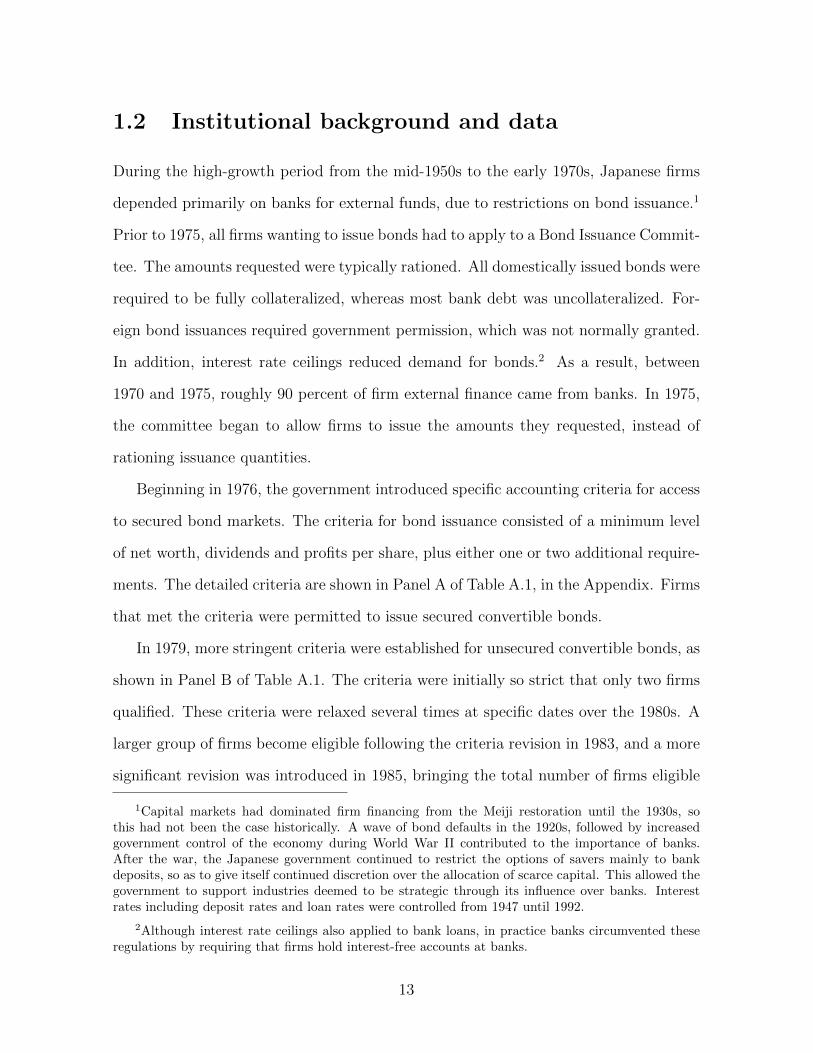
Over the 1980s, bond issuance increased rapidly, as shown in Figure 1.2. The total

number of qualified firms in the unsecured bond market is shown in Figure 1.3. As a

consequence of these reforms, firm borrowing patterns changed dramatically. In 1975,

for example, firms borrowed on average less than 5 percent of their debt from bond

markets, as shown in Figure 1.2. By 1990, the average was over 30 percent.

Importantly, the rules governing foreign exchange were also substantially relaxed in

1980. Foreign issuance had previously required explicit government permission. Re-

forms to the Foreign Exchange Law in 1980 changed this to allowing companies to

notify the Ministry of Finance, instead of requiring a formal permit (Kester, 1991).

Firms issuing foreign bonds still had to meet the relevant issuance criteria, but foreign

14

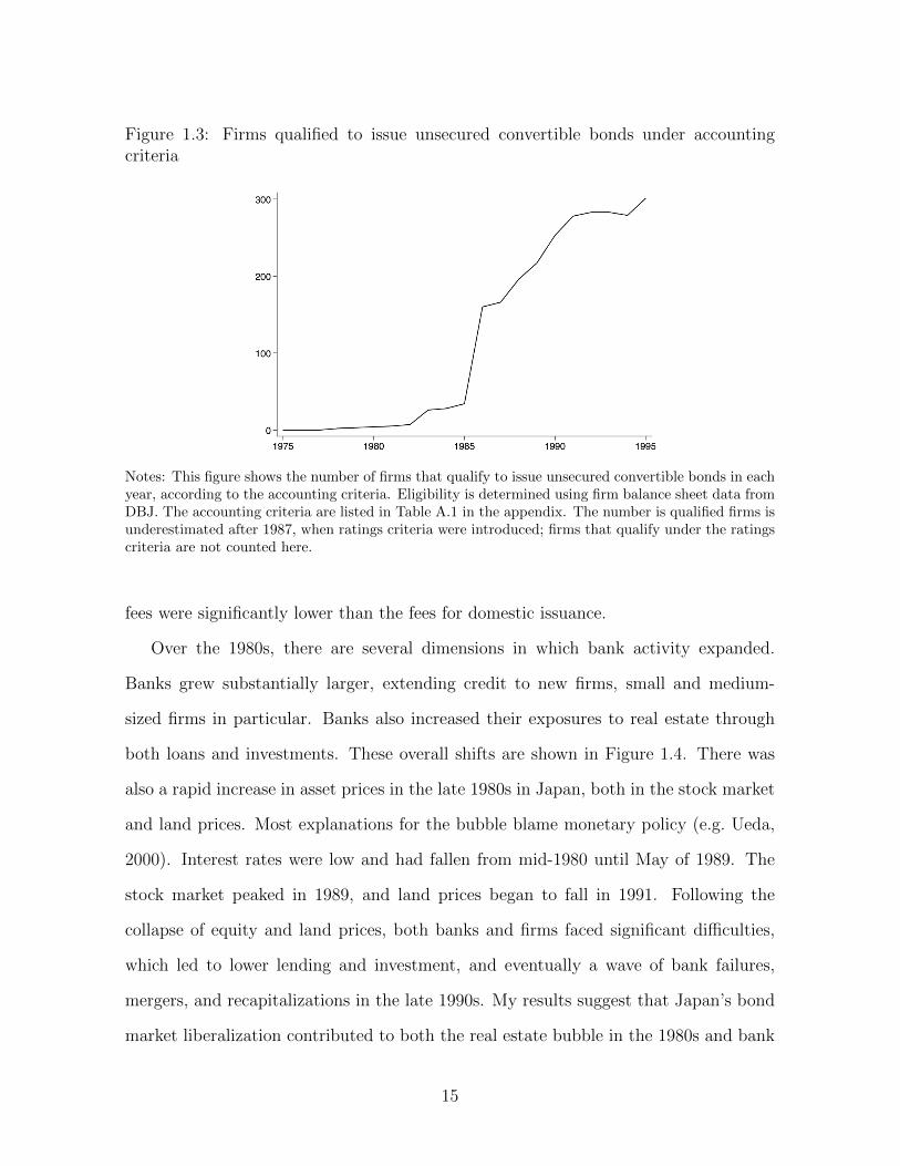
Figure 1.3: Firms qualified to issue unsecured convertible bonds under accountingcriteria

Notes: This figure shows the number of firms that qualify to issue unsecured convertible bonds in eachyear, according to the accounting criteria. Eligibility is determined using firm balance sheet data fromDBJ. The accounting criteria are listed in Table A.1 in the appendix. The number is qualified firms isunderestimated after 1987, when ratings criteria were introduced; firms that qualify under the ratingscriteria are not counted here.

fees were significantly lower than the fees for domestic issuance.

Over the 1980s, there are several dimensions in which bank activity expanded.

Banks grew substantially larger, extending credit to new firms, small and medium-

sized firms in particular. Banks also increased their exposures to real estate through

both loans and investments. These overall shifts are shown in Figure 1.4. There was

also a rapid increase in asset prices in the late 1980s in Japan, both in the stock market

and land prices. Most explanations for the bubble blame monetary policy (e.g. Ueda,

2000). Interest rates were low and had fallen from mid-1980 until May of 1989. The

stock market peaked in 1989, and land prices began to fall in 1991. Following the

collapse of equity and land prices, both banks and firms faced significant difficulties,

which led to lower lending and investment, and eventually a wave of bank failures,

mergers, and recapitalizations in the late 1990s. My results suggest that Japan’s bond

market liberalization contributed to both the real estate bubble in the 1980s and bank

15

Figure 1.4: Loans as a % of total bank lending

(a) Real estate (b) Small and medium firms

Notes: These figures show the percentage of total bank lending that is allocated to real estate firmsand small and medium firms over the period 1975-95. The percentages are calculated using the sumof bank-level financial reports from March 31 of each year shown, which is the fiscal year end for mostmajor banks in Japan.

problems in the 1990s.

1.2.1 Data

I use two main sources of data in this paper: firm-level financial data from the De-

velopment Bank of Japan (DBJ), and bank financial statements from Nikkei NEEDS

Financial Quest.

Firm financial data comes from the DBJ, which compiles regulatory findings from

the universe of listed firms in Japan. This data begins in 1956, and by 1980 includes

1,599 firms. By 1990, the sample has grown to 2,133. The detailed firm level data is

used to determine when firms become eligible to issue different types of bonds. In the

16

empirical analysis, I use the subset of firms that report a fiscal year end of March, which

is the majority of Japanese listed firms. This simplifies the analysis and is common

in other studies of Japan (e.g. Amiti and Weinstein, 2017). Because I use a subset of

firms, my estimates of the effects of the liberalization on banks are conservative.

In addition, the DBJ data includes disclosures on which banks lent to each firm in

each year, which allows the firm-level effects of the bond market liberalization to be

linked to the outcomes of banks they borrow from. This data is available beginning in

1982; in prior years, it is aggregated by bank type. In 1982, on average firms borrowed

from 14 lenders (median 11). By 1990, this had fallen to 10 (median 8).

Finally, bank balance sheet data is taken from the Nikkei NEEDS Financial Quest

database, to test the effect of liberalization on various bank outcomes and to control

for other bank characteristics.

1.3 Empirical evidence

In this section I show that firms that gained access to bond markets issued bonds as a

substitute for bank debt, and that as a result of the repayment of bank debt, banks lent

more to other firms. In particular, the bond liberalization contributed to bank lending

to small firms and real estate.

1.3.1 Firm level effects of bond liberalization

This section examines the impact of bond market liberalization on firms’ repayment

of bank debt, using the changes to the criteria for access to unsecured convertible

bond markets as an instrument for bond issuance. In looking at firm-level effects I

use an unbalanced panel of firms over the period 1977-1990, which includes the entire

liberalization period.

17

The first test is how the changes in policy that allowed certain firms to access the

unsecured convertible bond market affected bond issuance. Using the firm level data

and the criteria for access, I determine when each firm gained access to the unsecured

bond market, which is denoted by a dummy variable Accessj,t. By identifying when

each firm obtained access to new bond instruments, one can test for the effect of access

on bond issuance in a regression of the form:

Bj,t = λAccessj,t + ηj + δt + γ1Controlsj,t ∗ δt + e1j,t, (1.1)

where Bj,t is the ratio of bonds to total assets of firm j in time t, ηj is a firm fixed

effect, δt is a time fixed effect, and Controlsj,t is a vector of additional control variables,

interacted with year dummies. The control variables include firm characteristics such

as size, profitability, industry, region, and lenders, and are discussed in more detail

below.3

The main empirical test of this section estimates how bond issuance affects firms’

bank debt, using a regression of the form:

Lj,t = β Bj,t + ηj + δt + γ2Controlsj,t ∗ δt + e2j,t, (1.2)

where Lj,t is the bank debt to total assets ratio of firm j in time t. The coefficient on

Bj,t measures the extent to which bond issuance and bank debt are complements or

substitutes. Firm fixed effects control for time-invariant firm characteristics that affect

firms’ choice of bank debt. Time fixed effects filter out the effects of common macroeco-

nomic shocks on firms’ bank borrowing. Importantly, OLS estimates of equation (1.2)

do not have a causal interpretation, because a contraction in bank lending may cause

firms to issue bonds.

3Prior to the liberalization, some firms issued straight bonds, though the amounts were rationedup to 1975, and issuance volumes were low. Many firms had access to the secured convertible bondmarket, for which criteria were introduced in 1976. However, access to secured bond issuance did nothave a large impact upon introduction. Access to the domestic unsecured bond market is useful inthat it generates an increase in the probability of issuance, by granting firms access to the domesticunsecured market, as well.

18

To assess the effect of bond issuance on bank lending, I instrument for Bj,t using

the dummy variable that indicates whether firm j has access to bond markets in year

t, Accessj,t. This empirical strategy uses equation (1.1) as a first stage for equation

(1.2). This compares the outcomes of firms that get access to the unsecured convertible

bond market to firms without access, by looking at firms’ bond issuance and bank debt

before and after the policy changes are introduced. Because firms obtain access to the

bond market at different times, one needs to rule out other reasons why firms’ bank

borrowing may have changed, insofar as other drivers may be correlated with reforms to

the bond market. Further, because access is not randomly assigned, it is also necessary

to control for the characteristics that determine access.

To control for changes in banks’ credit supply, I run specifications that include

lender-year fixed effects. Firms’ lenders are reported in the DBJ data. Although firms

borrow from multiple banks, lender-year fixed effects are added for the banks from

which firms obtain the largest share of their loans, conditional on their share being

larger than 20 percent.4

Since there may also be changes in firm demand for bank debt, such as demand

shocks, I include specifications with industry-year and region-year fixed effects. Industry-

year fixed effects control for demand shocks that are industry specific. Region-time

dummies control for economic differences across Japan’s 47 prefectures, such as growth,

unemployment, demographics, and inflation.

Because the rules granting firms access to bond markets were based on firm charac-

teristics, firms that gained access to bond markets were larger and more profitable than

firms that did not. Other firm characteristics interacted with year dummies control for

the possibility that the change in bank debt is driven by firm characteristics in the

same years that certain types of firms gain access.

4This is analogous to using firm-year fixed effects to control for changes in firm-level credit demand,which also exploits the fact that firms borrow from multiple banks.

19

In addition, I run specifications that include as controls linear functions of the char-

acteristics that determine access, interacted with year dummies. Since access is based

on observable characteristics, this is analogous to a regression discontinuity design.5

To control for the effects of the observable characteristics on firm behavior, I include

the characteristics that are used to determine access as control variables (i.e. running

variables), interacted with year dummies. The key identification assumption here is

that there are no jumps in other firm characteristics around the thresholds for and

timing of the regulatory changes to access. Because there is a panel dimension to the

data, this implies that there are no changes in the trends for different groups of firms

that happen to coincide with the threshold of a particular policy change. Finally, I run

these same regressions on a sub-sample of the firms that are closer to the cutoffs, by

discarding very large and very small firms.

These specifications aim to capture the variation in bank borrowing that is at-

tributable to the liberalization policy. The interactions between year dummies and

firm characteristics control for the borrowing behavior of similar firms. The interpreta-

tion of the coefficient βIV is the effect of bond issuance on bank borrowing, for a firm

that gains access, relative to a firm in the same industry and region, of the same size

and profitability, controlling for bank credit supply.

Firm-level results

Table 1.2 shows the effect of bond market access on bond issuance. Access to domestic

unsecured convertible bond markets is associated with an increase in bonds over assets

of roughly 3 percentage points, on average, controlling for year and firm fixed effects,

as shown in column 1. Controlling for lender-year fixed effects has little effect on the

5Because bond issuance is not deterministic, but instead a probabilistic function of the accesscriteria, this corresponds to fuzzy RD. In other words, there are some firms that get access and do notissue bonds, so not every firm is a “Complier.”

20

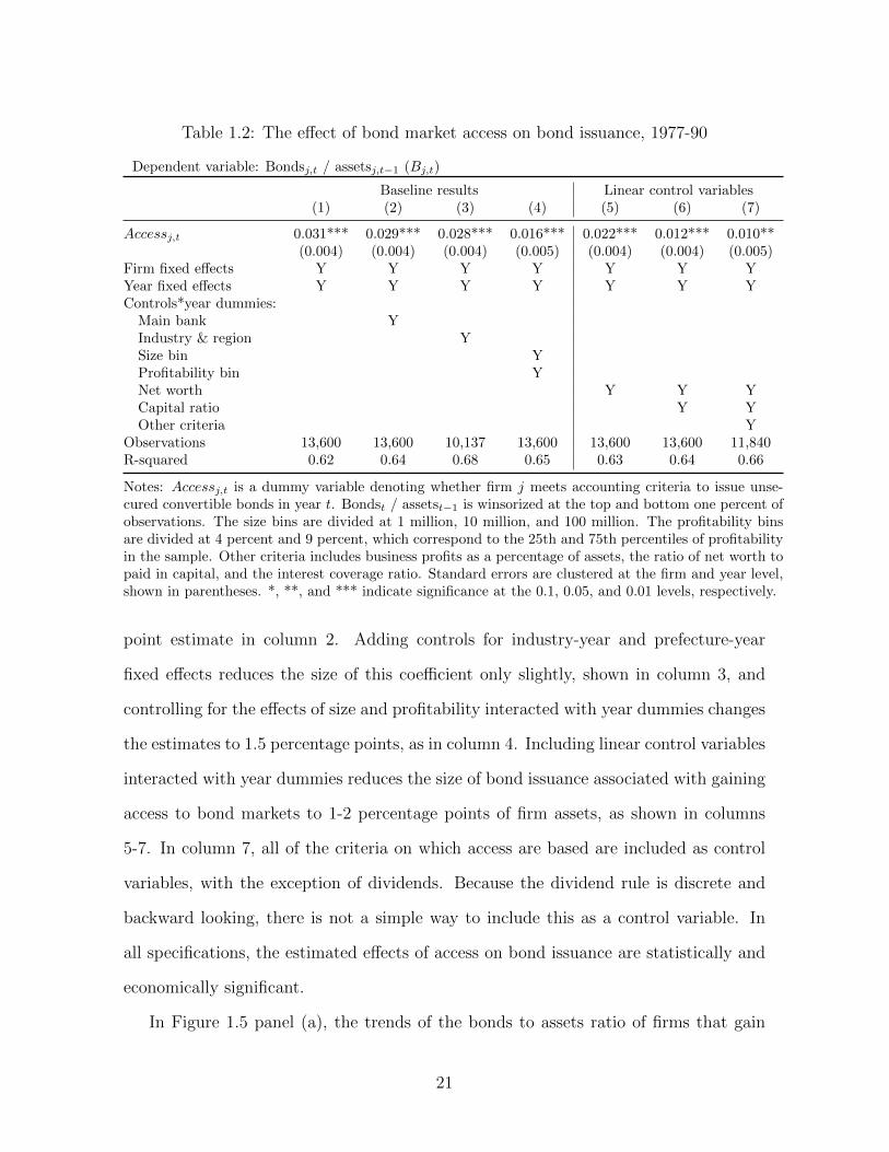
Table 1.2: The effect of bond market access on bond issuance, 1977-90

Dependent variable: Bondsj,t / assetsj,t−1 (Bj,t)

Baseline results Linear control variables(1) (2) (3) (4) (5) (6) (7)

Accessj,t 0.031*** 0.029*** 0.028*** 0.016*** 0.022*** 0.012*** 0.010**(0.004) (0.004) (0.004) (0.005) (0.004) (0.004) (0.005)

Firm fixed effects Y Y Y Y Y Y YYear fixed effects Y Y Y Y Y Y YControls*year dummies:

Main bank YIndustry & region YSize bin YProfitability bin YNet worth Y Y YCapital ratio Y YOther criteria Y

Observations 13,600 13,600 10,137 13,600 13,600 13,600 11,840R-squared 0.62 0.64 0.68 0.65 0.63 0.64 0.66

Notes: Accessj,t is a dummy variable denoting whether firm j meets accounting criteria to issue unse-cured convertible bonds in year t. Bondst / assetst−1 is winsorized at the top and bottom one percent ofobservations. The size bins are divided at 1 million, 10 million, and 100 million. The profitability binsare divided at 4 percent and 9 percent, which correspond to the 25th and 75th percentiles of profitabilityin the sample. Other criteria includes business profits as a percentage of assets, the ratio of net worth topaid in capital, and the interest coverage ratio. Standard errors are clustered at the firm and year level,shown in parentheses. *, **, and *** indicate significance at the 0.1, 0.05, and 0.01 levels, respectively.

point estimate in column 2. Adding controls for industry-year and prefecture-year

fixed effects reduces the size of this coefficient only slightly, shown in column 3, and

controlling for the effects of size and profitability interacted with year dummies changes

the estimates to 1.5 percentage points, as in column 4. Including linear control variables

interacted with year dummies reduces the size of bond issuance associated with gaining

access to bond markets to 1-2 percentage points of firm assets, as shown in columns

5-7. In column 7, all of the criteria on which access are based are included as control

variables, with the exception of dividends. Because the dividend rule is discrete and

backward looking, there is not a simple way to include this as a control variable. In

all specifications, the estimated effects of access on bond issuance are statistically and

economically significant.

In Figure 1.5 panel (a), the trends of the bonds to assets ratio of firms that gain

21

access to the unsecured convertible bond market by 1990 are compared to the firms

that do not gain access. The group of firms that gain access begin to issue bonds

earlier and in larger volumes than the firms without access. In panel (b), I plot the

estimated coefficients from a dynamic version of regression (1.1) that includes leads and

lags of the year in which firms gain access (t = 0): Bj,t =∑5

k=−5 λt−k Accessj,t−k +ηj +

δt + γ1Controlsj,t ∗ δt + e1j,t. Although firms have some ability to issue bonds before

gaining access to the unsecured market, upon gaining access, there is a significant and

persistent increase in the bonds to assets ratio of firms.

Similarly, in Figure 1.6 panel (a), the trends of the bank debt to assets ratio of firms

that gain access to the unsecured convertible bond market by 1990 are compared to the

firms that do not gain access. Although both groups of firms are deleveraging as they

come out of the high growth period which ends in the early 1970s, the group of firms that

does not gain access maintains a bank to asset ratio of roughly 25-30 percent throughout

the 1980s. In contrast, the firms that gain access to the bond market are able to continue

to shift away from banks, and reduce their bank debt to asset ratios to below 20 percent,

on average. In panel (b), I plot the estimated coefficients estimated from a dynamic

version of the reduced form regression that includes leads and lags of the time that firms

gain access (t = 0): Lj,t =∑5

k=−5 βt−k Accessj,t−k + ηj + δt + γ0Controlsj,t ∗ δt + e0j,t.

Although firms have some ability to anticipate that access will allow them to shift away

from banks, and begin reducing their bank debt in the year prior to when they gain

access, this shift continues after access is granted and persists for four years after firms

obtain access to the bond market.

Table 1.3 shows the elasticity of bank debt to bond issuance, as estimated using

regression (1.2). Using OLS, the relationship between bonds and bank loans is negative:

as shown in column 1, a one percentage point increase in bonds to assets is associated

with a 0.45 percentage point decrease in the ratio of bank loans to assets, controlling for

22

Figure 1.5: Bond issuance pre-trends and dynamics

(a) Average bonds to assets ratio (b) Dynamics

Notes: Panel (a) shows the average bond to assets ratio of firms that are granted access to the unsecuredconvertible bond market by 1990, compared to firms that do not obtain access. Panel (b) plots thecoefficients estimated from a dynamic version of regression (1.1) that includes leads and lags of the

year that firms gain access (t = 0): Bj,t =∑5

k=−5 λt−k Accessj,t−k +ηj +δt +γ1 Controlsj,t ∗δt +e1j,t.

Figure 1.6: Bank debt pre-trends and dynamics

(a) Average bank debt to assets ratio (b) Dynamics

Notes: Panel (a) shows the average bank debt to assets ratio of firms that are granted access to theunsecured convertible bond market by 1990, compared to firms that do not obtain access. Panel (b)plots the coefficients estimated from a dynamic version of the reduced form regression that includesleads and lags of the year that firms gain access (t = 0): Lj,t =

∑5k=−5 βt−k Accessj,t−k + ηj + δt +

γ0 Controlsj,t ∗ δt + e0j,t .

23

year and firm fixed effects. The point estimate from the regression in which I instrument

for the bonds to assets ratio using access to the unsecured bond market in column (2)

reveals that a bond issuance of one percent of assets due to the liberalization results

in a contemporaneous repayment of bank debt of one percent of assets. This estimate

is fairly stable to the inclusion of additional fixed effects, with the smallest estimated

coefficient being with the inclusion of industry-year and region-year fixed effects.

When linear functions of the main characteristics that determine access are included

in columns (6) and (7), the point estimates are similar. The most saturated specification

in column (8) is no longer statistically significant, but the point estimate also indicates

that the sizes of bond issuance and bank debt repayment are roughly proportional.

Finally, in Table 1.4, the same specifications are run using two smaller subsamples of

the data which exclude firms that are above or below specific sizes. It is not surprising

that after discarding more that two-thirds of the sample, the estimates are no longer

statistically significant. However, the point estimates remain very stable and indicate

that most bond issuance is being used to repay bank debt.

I also explore the effect of bond market access on other firm outcomes. This is done

using the regression specifications in equation (1.1), with other firm level-outcomes as

the dependent variables. The results of these regressions are shown in Appendix B.

Despite a fall in funding costs of approximately 1-2 percentage points (shown in panel

2 of Appendix B), firms’ total leverage does not increase (panel 3). There is also no

effect of bond market access on investment, employment, asset growth, or sales growth

(panels 4-7). In response to gaining access to bond markets, firms hold more cash,

less inventory, and seem to reduce their book equity (panels 8-10). These outcomes

are puzzling because they indicate that firms facing a decline in funding costs do not

undertake marginal investment projects.

24

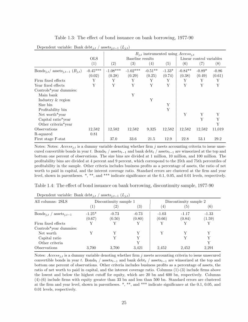
Table 1.3: The effect of bond issuance on bank borrowing, 1977-90

Dependent variable: Bank debtj,t / assetsj,t−1 (Lj,t)

Bj,t instrumented using Accessj,tOLS Baseline results Linear control variables(1) (2) (3) (4) (5) (6) (7) (8)

Bondsj,t/ assetsj,t−1 (Bj,t) -0.45*** -1.08*** -1.02*** -0.51** -1.33* -0.84** -0.89* -0.86(0.02) (0.28) (0.29) (0.25) (0.74) (0.38) (0.49) (0.61)

Firm fixed effects Y Y Y Y Y Y Y YYear fixed effects Y Y Y Y Y Y Y YControls*year dummies:

Main bank YIndustry & region YSize bin YProfitability bin YNet worth*year Y Y YCapital ratio*year Y YOther criteria*year Y

Observations 12,582 12,582 12,582 9,325 12,582 12,582 12,582 11,019R-squared 0.81First stage F-stat 37.0 33.6 21.5 12.9 22.8 53.1 29.2

Notes: Notes: Accessj,t is a dummy variable denoting whether firm j meets accounting criteria to issue unse-cured convertible bonds in year t. Bondst / assetst−1 and bank debtt / assetst−1 are winsorized at the top andbottom one percent of observations. The size bins are divided at 1 million, 10 million, and 100 million. Theprofitability bins are divided at 4 percent and 9 percent, which correspond to the 25th and 75th percentiles ofprofitability in the sample. Other criteria includes business profits as a percentage of assets, the ratio of networth to paid in capital, and the interest coverage ratio. Standard errors are clustered at the firm and yearlevel, shown in parentheses. *, **, and *** indicate significance at the 0.1, 0.05, and 0.01 levels, respectively.

Table 1.4: The effect of bond issuance on bank borrowing, discontinuity sample, 1977-90

Dependent variable: Bank debtj,t / assetsj,t−1 (Lj,t)

All columns: 2SLS Discontinuity sample 1 Discontinuity sample 2(1) (2) (3) (4) (5) (6)

Bondsj,t / assetsj,t−1 -1.25* -0.73 -0.73 -1.03 -1.17 -1.33(0.67) (0.50) (0.80) (0.66) (0.84) (1.59)

Firm fixed effects Y Y Y Y Y YControls*year dummies:

Net worth Y Y Y Y Y YCapital ratio Y Y Y YOther criteria Y Y

Observations 3,700 3,700 3,421 2,452 2,452 2,291

Notes: Accessj,t is a dummy variable denoting whether firm j meets accounting criteria to issue unsecuredconvertible bonds in year t. Bondst / assetst−1 and bank debtt / assetst−1 are winsorized at the top andbottom one percent of observations. Other criteria includes business profits as a percentage of assets, theratio of net worth to paid in capital, and the interest coverage ratio. Columns (1)-(3) include firms abovethe lowest and below the highest cutoff for equity, which are 20 bn and 600 bn, respectively. Columns(4)-(6) include firms with equity greater than 33 bn and less than 500 bn. Standard errors are clusteredat the firm and year level, shown in parentheses. *, **, and *** indicate significance at the 0.1, 0.05, and0.01 levels, respectively.

25

1.3.2 Spillovers via the banking system

In this section, I estimate how the shift away from banks among firms issuing bonds

led to a positive liquidity shock for banks, and how this affected bank lending. By

exploiting the timing of the changes in liberalization policy and the relative exposure

of banks to firms gaining access, these shocks are plausibly exogenous to other drivers

of changes in the loan portfolio of banks. For this analysis I focus on the sub-period

from 1983 to 1987. Specific data on the identity of matched borrower-lender pairs is

not available until 1982, and I focus on the five year period following this, prior to the

serious bubble years.

To construct a measure of the size of the repayment shock affecting each bank,

I first calculate the predicted repayments of each firm and then aggregate them into

repayments at a bank level, using the network of bank-firm lending relationships. A

firm’s predicted repayment is calculated as follows. For firms that gain access to the

bond market, the predicted issuance Bj,t|Accessj,t = 1 estimated in regression (1.1) is

multiplied by the repayment coefficient estimated using regression (1.2):

∆Lj,t = βIV ∗[Bj,t|Accessj,t = 1

].

Predicted issuance is used instead of actual issuance in constructing the predicted

repayments, because predicted issuance is less likely to be correlated with bank-level

variables. The main identifying assumption here is that the time and cross-sectional

variation in banks’ exposure to firms that gain access to the bond market is uncorrelated

with other factors that affect bank lending.

At the bank level, the repayment shock Ri,t is calculated as the sum of predicted

repayments made by firms that borrowed from bank i in period t−1, denoted j ∈Mi,t−1,

and that gained access to the bond market, divided by total bank lending to listed firms:

Ri,t =

∑j∈Mi

Predicted repaymentsj,t

Total loansi,t−1

=

∑j∈Mi|Aj=1 Θij,t−1∆Lj,t ∗ Assetsj,t−1∑

j∈Mi,t−1`ij,t−1

,

26

where `ij is the nominal size of a loan from bank i to firm j. To obtain a nominal firm-

level repayment, the predicted repayment ∆Lj,t is multiplied by lagged firm assets.

These repayments are also weighted by the share of bank i in firm j’s total borrowing:

Θij =`ij∑

i∈Mj`ij

. For example, a firm that borrows equal amounts from two banks will

have Θij = Θi′j = 0.5, which scales the amount each bank is predicted to be repaid

from that firm to half of the nominal total.6

One test of the effect of the repayment shocks on bank lending is to regress the

growth rate of lending between bank i and firm j on the bank shock Ri,t:

∆ log `ij,t = βRi,t + ηj,t + εij,t. (1.3)

where ηj,t is a firm-year fixed effect. The firm-year fixed effects address the concern that

results are being driven by demand shocks affecting firms that happen to borrow from

shocked banks. The coefficient on Ri,t measures the effects of the bank-level repayment

shock at bank i on firm j, relative to firm j’s borrowing from other unshocked banks.

A positive coefficient indicates that a bank shock is associated with higher lending,

relative to firm borrowing from other banks without repayment shocks.

In linking the bond liberalization shocks to bank outcomes, the key identifying

assumption is that the timing and relative exposure of banks to firms that gain access

to bond markets is uncorrelated with other shocks that affect bank lending. In other

words, banks did not lend to these large, profitable clients because of characteristics of

the rest of their loan portfolio. Although banks that lend to large, profitable firms and

are therefore disproportionately affected by the bond market liberalization may lend to

different types of firms than other banks, the within-firm comparisons provide a good

6One concern is whether firms indeed repay their banks in proportion to the past lending shares.Since firms borrowed from many banks (14 on average in 1982), it is possible that strategic consider-ations were taken into account when firms decided which banks to repay. While this would increasethe explanatory power of the repayment shocks, it is also more likely to be endogenous to bank char-acteristics.

27

test of the supply side effects of the repayment shocks. Using predicted rather than

actual bond issuance in constructing the shocks furthers this argument.

Another test of where capital allocated as a result of the liberalization is whether

the repayment shocks cause banks to lend more to other specific groups of firms or

industries. Regression (1.4) tests whether the repayment shocks are associated with

different values of a bank-level variable ∆ log Yi,t:

∆ log Yi,t = β Ri,t + ζi + δt + ei,t, (1.4)

where Ri,t is the repayment shock described in the previous section, ζi is a bank fixed

effect, and δt is a time fixed effect. The outcomes I focus on for ∆ log Yi,t are the change

in the log of lending to small and medium firms and real estate firms.

Bank-level results

On average, the actual bond issuance that can be traced back to banks totals three

percent of bank loans to listed firms. The repayment shocks are constructed using the

coefficients in column 1 of Table 1.2 in the years each firm has access, multiplied by

lagged firm assets. Given the results at the firm level, I construct firm level repayments

by assuming that each yen of this issuance was repaid. Using the credit registry to

determine which firms borrowed from what banks, and the shares of each predicted

repayment to attribute to each bank, the predicted firm-level repayments are added up

at the bank level in each year. The repayment shocks predicted from the bond market

liberalization range between 0 and 6 percent of loans, and are summarized in Table 1.5.

The average repayment shock associated with access to the unsecured convertible bond

market is 0.5 percent of total lending to listed firms. Although the average shocks are

small, certain banks were more affected than others.

Table 1.6 compares characteristics of banks by the tercile of repayment shock that

they are subject to. Although banks in the first tercile of shocks are smaller than

28

Table 1.5: Repayment shocks, 1983-87 (%)

Type Mean Median p75 p95 N

Long-term credit 0.7 0.1 1.7 2.2 15City bank 0.9 0.3 1.6 3.2 65Trust bank 0.7 0.1 1.5 2.0 35Regional bank 0.4 0.0 0.8 1.9 286

Total 0.5 0.0 1.1 2.1 401

Notes: This table shows summary statistics for the repayment shocksassociated with bond market liberalization calculated for banks between1983 and 1987. The shocks are scaled using total loans to listed firms.

banks in the other terciles, on other observable characteristics the banks are closely

comparable. They have similar levels of leverage, return on assets, and profitability. In

addition, the shares of lending to real estate and small firms are relatively close, and

there are almost no changes in the shares of loans to these sectors in the two years prior

to the period in which the repayment shocks are calculated.

Table 1.7 shows the effects of the repayment shock on bank lending to listed firms,

which corresponds to regression (1.3). In columns 1 and 2, the sample includes firms

without access to unsecured bond markets. Column 1 shows that a one percentage

point increase in the repayment shock is associated with an increase in borrowing of

2 percentage points relative to its borrowing from an unaffected bank, controlling for

firm-year fixed effects. If instead we control for firm and year fixed effects, the size of

the coefficient is essentially unchanged. Columns 3 and 4 restrict the sample further

to firms with no bonds at all, and finds smaller but still statistically and economically

significant responses to the shock. The size of the coefficients with and without firm-

year fixed effects are roughly the same in size, which indicates that it is unlikely that

demand shocks are positively correlated with the repayment shocks.

Table 1.8 shows the effect of the repayment shock on lending to real estate firms and

small and medium enterprises. A one percentage point increase in the repayment shock

is associated with an increase in lending to real estate firms of 2-3 percentage points,

29

Table 1.6: Balancing of covariates in the sample, 1983-87 (%)

Quantile of Ri,t Memo:1 2 3 std. dev.

Total Assets (Utr) 1,390 10,010 7,360 6,761Leverage 38.1 42.5 39.4 10.6ROA (%) 0.52 0.48 0.53 0.15NIM (%) 2.2 1.1 1.6 0.6

Real estate loans / total, 1982 (%) 6.9 7.7 6.4 4.0∆ share, 1980-1982 (%) 0.5 0.1 0.1 0.9

Small firms loans / total, 1982 (%) 79.9 47.8 60.0 19.0∆ share, 1980-1982 (%) -0.3 -0.9 -0.7 0.4

Notes: This table compares the characteristics of banks by tercile of repaymentshocks Ri,t in the sample.

as shown in columns 1 and 2. The effect on lending to small and medium firms is 1-2

percentage points, on average, and still statistically significant, as shown in columns 3

and 4.

Figure 1.7 compares the lending behavior of banks with positive repayment shocks

to those with no repayments. While the patterns of lending are similar in the early

years of the liberalization, there is a substantial divergence between the growth rates

of lending to real estate beginning in 1985, and to small and medium firms beginning

in 1986.

The evidence presented in this section demonstrates that the bond market liberal-

ization in Japan led more firms to issue bonds and pay back bank debt. Among banks,

these repayments led to greater lending to other listed firms, as well as lending to small

firms and real estate. This evidence indicates that Japan’s bond market liberalization

contributed to the economic problems that Japan began to face a few years later, fol-

lowing the collapse of asset prices and the stock market bubble. Banks’ exposures to

real estate in the late 1980s have been shown to predict loan delinquency rates and

declines in lending in the 1990s (Hoshi, 2001; Gan, 2007b). However, to explore the

aggregate implications of bond market liberalization, to determine the key factors driv-

30

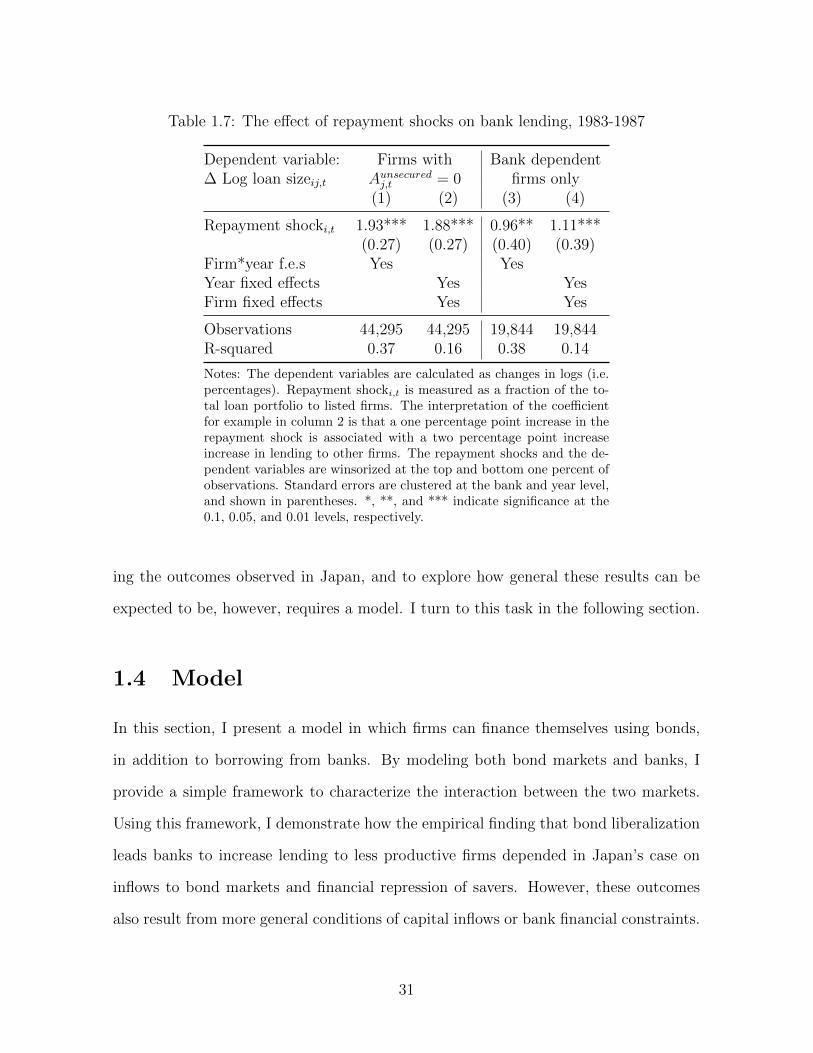
Table 1.7: The effect of repayment shocks on bank lending, 1983-1987

Dependent variable: Firms with Bank dependent∆ Log loan sizeij,t Aunsecuredj,t = 0 firms only

(1) (2) (3) (4)

Repayment shocki,t 1.93*** 1.88*** 0.96** 1.11***(0.27) (0.27) (0.40) (0.39)

Firm*year f.e.s Yes YesYear fixed effects Yes YesFirm fixed effects Yes Yes

Observations 44,295 44,295 19,844 19,844R-squared 0.37 0.16 0.38 0.14

Notes: The dependent variables are calculated as changes in logs (i.e.percentages). Repayment shocki,t is measured as a fraction of the to-tal loan portfolio to listed firms. The interpretation of the coefficientfor example in column 2 is that a one percentage point increase in therepayment shock is associated with a two percentage point increaseincrease in lending to other firms. The repayment shocks and the de-pendent variables are winsorized at the top and bottom one percent ofobservations. Standard errors are clustered at the bank and year level,and shown in parentheses. *, **, and *** indicate significance at the0.1, 0.05, and 0.01 levels, respectively.

ing the outcomes observed in Japan, and to explore how general these results can be

expected to be, however, requires a model. I turn to this task in the following section.

1.4 Model

In this section, I present a model in which firms can finance themselves using bonds,

in addition to borrowing from banks. By modeling both bond markets and banks, I

provide a simple framework to characterize the interaction between the two markets.

Using this framework, I demonstrate how the empirical finding that bond liberalization

leads banks to increase lending to less productive firms depended in Japan’s case on

inflows to bond markets and financial repression of savers. However, these outcomes

also result from more general conditions of capital inflows or bank financial constraints.

31

Table 1.8: The effect of repayment shocks on bank lending, 1983-1987

Dependent variable:∆ Log loans to Real estate Small/medium firms

(1) (2) (3) (4)

Repayment shocki,t 3.3*** 2.3** 2.5*** 1.3**(1.0) (1.0) (0.8) (0.6)

Year fixed effects Yes Yes Yes YesBank fixed effects Yes Yes

Observations 393 393 400 400R-squared 0.13 0.56 0.09 0.60

Notes: The dependent variables are calculated as changes in logs (i.e.percentages). Repayment shocki,t is measured as a fraction of the to-tal loan portfolio to listed firms. The interpretation of the coefficientfor example in column 2 is that a one percentage point increase in therepayment shock is associated with a two percentage point increase in-crease in lending to real estate firms. The repayment shocks and thedependent variables are winsorized at the top and bottom one percentof observations. Standard errors are clustered at the bank and yearlevel, and shown in parentheses. *, **, and *** indicate significance atthe 0.1, 0.05, and 0.01 levels, respectively.

1.4.1 Setup

There are three types of agents in the model: entrepreneurs, banks, and foreign in-

vestors.

Entrepreneurs

Entrepreneurs exist on a joint distribution G(a, z) of assets a and productivities z.

Each unit decides whether to save, invest without borrowing, or borrow bank debt `

and bonds b to invest, in which case their capital is:

k = `+ b+ a. (1.5)

Production is constant returns to scale, so output is the product of capital and en-

trepreneurs’ productivity z. Output is homogenous.

32

Figure 1.7: Comparison between affected and unaffected banks

(a) ∆ log Real estate lending (b) ∆ log Lending to small firms

Notes: Panel (a) shows the average change in the log of lending to real estate firms of banks withpositive repayment shocks compared with the average among banks with no repayments, and panel(b) shows the comparison for the average change in the log of lending to small and medium firms.While the patterns of lending are similar in the early years of the liberalization, there is a substantialdivergence between the growth rates of lending to real estate beginning in 1985, and to small andmedium firms beginning in 1986.

Firms’ total borrowing is limited to some multiple of the value of their assets:

`+ b ≤ θa, (1.6)

where θ > 1 represents in a reduced form way the fact that firms’ demand for external

finance is bounded.7 This constraint limits the total demand for debt of firms.

The gross interest rate on bank loans is r. Bond funding is cheaper than bank loans,

assumed to be equal to the interest rate paid on deposits, rf .8 However, to gain access

7Another way to limit firms’ demand for external funds would be for production to be decreasingreturns to scale. However, since in the empirical findings firms do not borrow more in response to adecline in borrowing costs, the constraint in equation (1.6) is consistent with the empirical findings ofSection 1.3.

8An interest rate on bonds equal to the risk-free rate is of course a simplification. The spreadon bonds over the risk-free rate varies over time and has been shown to exceed the interest rate onloans in times of stress. However, adding bond spreads is inessential to the main results. A model ofhouseholds with mean-variance preferences and endogenous bond spreads is Adrian, Colla, and Shin(2013).

33

to bond markets, firms must pay a fixed cost f . This prevents small firms from issuing

bonds, and can be thought of as either the actual costs involved in arranging a bond

issuance, or a reduced form way to represent the size threshold necessary for bonds to

be sufficiently liquid to attract investor interest.9

All firms that borrow require a bank to monitor production. Bondholders do not

monitor. There is a cost to monitor firms, denoted m(a), and banks’ nominal return on

a loan ` must be at least as large as banks’ monitoring cost. This places an additional

constraint on corporate debt structure, as a function of loan size and the spread of the

lending rate over the deposit rate:

(r − rf )` ≥ m(a). (1.7)

The monitoring cost is increasing in the size of entrepreneurs’ assets, m′(a) > 0,

m′′(a) ≤ 0. This represents the operational costs a bank incurs, such as loan offi-

cer salaries. Banks’ minimum loan sizes could imply that some firms are too small to

borrow from banks. However, this does not play an interesting role in the subsequent

analysis, so in what follows I assume that m(0) = 0. This reduced form constraint pins

down the mix of funding demanded by firms.10

If an entrepreneur decides not to produce, they can save in banks or invest in bonds.

The return on savings is rf . Since the return on bonds is the same as bank deposits,

households are indifferent between the two assets. Aggregate savings S are invested in

both bank deposits D and bonds B:

S = D +B, (1.8)

9Blackwell and Kidwell (1988) show that public debt has greater fixed costs, and that this makeslarge firms more likely to issue public debt.

10That all firms that borrow must have a bank loan is motivated by the substantial theoreticalevidence on the monitoring role of banks (e.g. Diamond, 1991), the complementarity between informed(i.e. bank) and uninformed capital (Holmstrom and Tirole, 1997), and the flexibility to renegotiate infinancial distress (Bolton and Scharfstein, 1996) - against the lower cost of bonds. Empirically, mostsmall firms borrow from banks, and banks are responsible for arranging bond issuances.

34

where capital letters are used to denote aggregate outcomes. Aggregate loan demand

is denoted by L, and total bond supply BS.

Entrepreneurs choose whether to save or invest in order to maximize:

max{b,m}

{za, zk − r`− rfb− f · 1{b > 0}, rfa} , (1.9)

where the first term is the return to investing without debt (i.e. self-financing), the

second term is the return to borrowing and investing, and the third term is the return

to saving. This choice depends on the interest rates r and rf , which are taken as given

by entrepreneurs, and is subject to the capital constraint equation (1.5), the borrowing

constraint (1.6), and the minimum loan size (1.7).

Banks

Banks have an endowment of initial equity E, raise deposits, and lend to firms. The

bank balance sheet consists of bank loans L on the asset side, and the sum of household

deposits D, foreign deposits DF , and equity E on the liability side:

L = D +DF + E. (1.10)

Banks require both that firm borrowing is no greater than a multiple of their existing

assets in equation (1.6), and that their loans generate enough revenue to cover the

associated monitoring cost in equation (1.7). In the spirit of Gertler and Kiyotaki

(2010), the deposits banks can attract are limited to a multiple of bank equity:

D +DF ≤ φE, (1.11)

where φ > 0 is a bank borrowing constraint. When equation (1.11) binds, the banks’

balance sheet equation (1.10) becomes:

L = (φ+ 1)E. (1.12)

35

This constraint implies either that banks have a limited capacity to intermediate domes-

tic savings, in which case some domestic savings are invested abroad, or else that banks

may raise more deposits from foreign sources than they are able to raise domestically.

The banking sector is perfectly competitive and chooses the supply of loans L and

deposit demand D to maximize profits:

Π = rL− rfD −M(L), (1.13)

subject to the balance sheet identity (1.10) and where M(L) is the total monitoring

cost associated with the loan portfolio L.

Foreign investors

Foreign investors play a reduced role in the model. When foreign deposits are permit-

ted, foreign investors provide bank deposits DF up to the maximum allowed by the

constraint in equation (1.11). I consider cases in which DF is exogenously given at

some level below the maximum.

Foreign demand for bonds adds to domestic bond demand:

BS = B +BF , (1.14)

which allows consideration of cases in which bond liberalization interacts directly with

capital inflows. Similarly to foreign bank deposits, I consider cases in which BF is

given. In the absence of such assumptions, bond inflows could entirely displace domestic

investors in bond markets.

1.4.2 Equilibrium

In a competitive equilibrium, entrepreneurs and banks maximize subject to constraints,

and the markets for loans, bonds, and savings clear. Bank equity E, the risk free rate

rf , and inflows DF and BF are taken as given, and r is determined in equilibrium.

36

To see this, note that the sum of bank loans and bond supply must equal the sum of

household savings, bank equity, foreign deposits, and foreign demand for bonds:

L+BS = S + E +DF +BF . (1.15)

The demand for funds is decreasing in r, because fewer entrepreneurs choose to borrow

when the interest rate is high. The supply of savings is increasing in rf : higher returns

on savings discourage entrepreneurs from production. Since rf is taken as given, in

equilibrium r rises or falls until investment demand equal savings plus bank equity.

Inflows to banks or bonds, DF and BF , add to the total supply of capital in the

economy; this reduces the interest rate.

In an economy without bond markets, i.e. f = ∞, all entrepreneurs with produc-

tivity higher than rf invest in production, and those with productivity greater than r

borrow to invest. When f = ∞, entrepreneurs’ decision to save or invest depends on

the return to saving, relative to the profits of production funded with or without bank

debt. Comparing the returns to investing only one’s own assets to the returns to saving

yields a simple rule to invest in production if z > rf . Comparing the returns to invest-

ing without bank debt to the returns to investing using bank debt leads entrepreneurs

to borrow if their productivity exceeds the interest rate on bank debt, i.e. z > r. These

thresholds are plotted in (a, z) space in panel (a) of Figure 1.8, assuming finite bounds

on both entrepreneurs’ assets [a, a] and productivity [z, z].

When bond markets exist, i.e. f <∞, firms pay to access bond markets if the cost

savings that result from bond issuance exceed the fixed cost of issuing a bond:

rθa−[rm(a)

r − rf+ rf

(θa− m(a)

r − rf

)]≥ f.

Using a linear monitoring cost function m(a) = m1a, this can be simplified to a decision

to issue bonds if assets are larger than a∗:

a ≥ a∗ ≡ f

θ(r − rf )−m1

. (1.16)

37

Only entrepreneurs with sufficient assets can issue enough bonds to make paying the

fixed cost worthwhile. For firms with assets a below the threshold a∗, the participation

decision remains to invest if z > r. However, for firms with enough assets to enter the

bond market a ≥ a∗, the lower average cost of funding encourages lower productivity

firms to enter production, leading to a decision to invest if:

z > z∗(a) ≡ rf +m(a) + f

θaif a ≥ a∗. (1.17)

When both bank debt and bonds are available, the decision to invest depends on not

only productivity but also assets, which allow firms to take advantage of the lower cost

of bond finance. The entrepreneurs’ decisions with both funding options are shown in

Figure 1.8 panel (b). In contrast to panel (a), entrepreneurs with high productivity

and high assets borrow from banks and issue bonds. The advantage conferred by size

decreases the borrowing threshold for large firms, leading to a lower threshold z∗ < r

that is decreasing in the level of assets. As a consequence, the interest rate also affects

the mix of funding demanded by a subset of firms. When r rises, demand for bank

loans decreases because some entrepreneurs no longer borrow from banks, and because

firms switch to issuing bonds. Firms with a > a∗ and z > z∗ continue to borrow from

banks, because banks’ monitoring costs lead to a minimum bank loan size in equation

(1.7).

The aggregate outcomes in the economy are expressed as functions of the distribu-

tion of entrepreneurs’ assets and productivity G(a, z). Savings are given by:

S =

∫ a

a

∫ rf

z

a dG(a, z), (1.18)

while the demand for bank debt is:

L =

∫ a∗

a

∫ z

r

θa dG(a, z) +

∫ a

a∗

∫ z

z∗(a)

m(a)

r − rfdG(a, z), (1.19)

where the first term is the bank debt demanded by firms that do not issue bonds, and

the second term is the sum of the minimum loan sizes demanded by firms with mixed

38

Figure 1.8: Entrepreneurs’ decisions

az

z

a

r

rf

Savers

Self-financing firms

Firms with bank debt

(a) Bank debt only

az

z

a

r

z∗

a∗

Savers

rf

Bankdebt Bank debt

and bonds

Self-financing firms

(b) Bank debt and bonds

Notes: Panel (a) shows the decisions of a joint distribution of entrepreneurs that are heterogenous inassets and productivity, in the case when bond issuance is infinitely costly, i.e. f = ∞, and banksare the only source of capital. Panel (b) shows the pattern of entrepreneurs’ decisions for a finitef ′ < f =∞.

funding structures. The supply of bonds comes from firms that mix bonds and bank

loans:

BS =

∫ a

a∗

∫ z

z∗(a)

θa− m(a)

r − rfdG(a, z), (1.20)

where each firm issues the difference between the maximum in equation (1.6) and the

minimum bank share in equation (1.7). Total demand for funds in the economy is

the sum of demand for bank loans and bond issuance, which together add up to each

entrepreneurs’ borrowing constraint.

Total output in the economy is:

Y =

∫ a

a

∫ min{r,z∗}

rf

za dG(a, z) +

∫ a

a

∫ z

min{r,z∗}zθa dG(a, z), (1.21)

which includes both the output of self-financed entrepreneurs (first term) and the output

of firms that borrow up to θ and produce (second term). An expression for aggregate

39

productivity is:

Z =Y

min{∫ a

a

∫ zza dG(a, z) +DF , (φ+ 1)E

}+BF

(1.22)

which is the ratio of output to inputs, so the denominator includes both domestic

capital and any foreign inflows.

In this economy, the optimal allocation of capital absent borrowing constraints

would be for the highest productivity firms to invest all of the capital in the economy.

In this setting, misallocation arises because firms’ bounded demand for debt θ prevents

capital from being allocated optimally. As the threshold for entry into borrowing mar-

kets falls, this decreases productivity Z, because the marginal borrowers entering have

lower productivity than existing market participants. In addition, the bias towards

large firms introduced by bond markets leads to further declines in productivity, or

equivalently, increases in misallocation.

1.4.3 Results

To consider the impact of a bond market liberalization, I compare the effect of a de-

cline in the fixed cost of issuing bonds from f = ∞ to some lower f ′ < f . Since

the equilibrium described above is static, the results are discussed using comparative

statics.11

First, assume the economy is closed, i.e. DF = BF = 0, and that banks are

unconstrained, i.e. S < φE. Under these assumptions, the main effect of bond market

liberalization is to increase the demand for funds of marginal firms that can access both

banks and bond markets. Absent additional capital, this diverts funds from smaller

firms, through an increase in the lending rate. This result is formalized in Proposition

1.1.

11Dynamics can be considered as a sequence of static equilibria with evolving bank equity andentrepreneur asset holdings.

40

Proposition 1.1. Unconstrained closed economy bond market liberalization. If DF =

BF = 0 and S < φE, (i) B = BS, and (ii) a reduction in the fixed cost of issuing bonds

to f ′ < f =∞:

1. decreases a∗ (new issuers);

2. decreases z∗ (marginal large firms enter);

3. increases r (marginal small firms exit);

4. decreases Y (output); and,

5. decreases Z (productivity).

The results of the introduction of a bond market is on shown graphically in panel

(a) of Figure 1.9. Decreasing the fixed cost of bond issuance leads more firms to issue

bonds. Firms with a > a∗ and z > r issue bonds, and use the bonds as a substitute

for bank debt. Taken alone, the shift in a∗ has no impact on the interest rate because

savers are indifferent between bank deposits and bonds.

However, marginal entrepreneurs with many assets begin to borrow from banks and

bond markets instead of self-financing, because the lower fixed cost improves the return

to borrowing and investing. This arises because the threshold z∗ at which large firms

borrow is lower than r, and increases overall demand for loans and bonds. The increase

in demand leads to an increase in the equilibrium interest rate r, which discourages

marginal small firms from borrowing. Higher bank lending rates also encourage addi-

tional firms to issue bonds instead of bank debt, which adds to the downwards shift in

the bond issuance cutoff a∗.

Because the closed economy bond market reallocates capital from small produc-

tive firms to less productive large firms, all else equal, the bond market liberalization

decreases both output and aggregate productivity.

To more closely capture the dynamics of the bond market liberalization in Japan,

now consider modified version of Proposition 1.1. As the fixed cost of issuing bonds is

41

Figure 1.9: Bond market liberalization

arf

z

a

r

r′

z∗

a∗

(a) Unconstrained closed economy

arf

z

a

r

r′

z∗

a∗

(b) Constrained/open economy

Notes: The solid lines represent the decision thresholds of entrepreneurs for f = ∞, and the dashedlines represent the equilibrium result for f ′ < f . Panel (a) shows the effect of a liberalization in whichthere is no foreign investment and banks are unconstrained. In contrast, panel (b) shows the outcomewhen domestic savers hold only deposits, and foreign investors purchase all bonds.

reduced to f ′ < f = ∞, consider the impact of also allowing inflows. There are three

separate sufficient conditions for the bond market liberalization to lead to a decline

in r instead of an increase: financial repression (B = 0) and inflows to the bond

market (BF > 0), inflows to banks (DF > 0), or if banks are domestically constrained

(S > φE). This result is formalized in Proposition 1.2.

Proposition 1.2. Constrained bond market liberalization. If B = 0 and BF > 0, or

DF > 0, or S > φE, a reduction in the fixed cost of issuing bonds to f ′ < f =∞:

1. decreases a∗ (new issuers);

2. decreases z∗ (marginal large firms enter);

3. decreases r (marginal small firms enter);

4. increases Y (output); and,

42

5. decreases Z (productivity).

These results are shown in panel (b) of Figure 1.9. As in the case of a closed

economy liberalization, the assets threshold a∗ for bond issuance falls because of the

fall in f , and more firms issue bonds. Firms that switch from bank to bond financing

repay bank debt, and marginal large firms choose to enter the borrowing market as f

declines, as before. These firms demand bank loans and issue bonds, but their demand

for bank debt is less than the repayment of bank debt by firms issuing bonds. This

leads to a decline in demand for loans.

To make clear the effect of bond inflows, consider the case in which domestic savers

are not permitted to invest in bonds, i.e. B = 0, and foreign investors purchase bonds.

When savers can frictionlessly substitute investing in bonds for bank deposits, this

reallocates savings from banks to bond markets. When B = 0, however, this sets S = D

in equation (1.8), and all bonds are purchased by foreign investors, i.e. BS = BF .

Preventing savers from substituting from deposits to bonds leads to excess deposits

relative to declining loan demand. A fall in the lending rate brings the market back

into equilibrium, but necessitates more lending to entrepreneurs with low productivity.

Although output rises due to the increases in entrepreneurs who borrow and invest,

productivity falls.

In the more general case when BF > 0 but B 6= 0, foreign inflows to the bond

market still cause some savers to be crowded out of investing in bonds. This leads to

the same effect as described above, although to a lesser extent if domestic households

have some ability to shift savings into the bond market.

The bond liberalization leads to spillovers because banks lose a portion of their

loan volume to bond issuance, and then hold excess deposits relative to their remaining

portfolio of loans. Returning deposits to households is ruled out by the exogenous risk-

free rate. Absent other safe assets or investment options, and assuming firms’ total

43

borrowing remains unchanged, banks lend to marginal firms.12

These outcomes are in fact isomorphic to a bond market liberalization in which

banks are constrained, in which equation (1.11) binds because either S > φE orDF > 0.

When constrained banks limit productive investment, bond market liberalization allows

more firms to invest. Substitution away from banks frees up bank funds to lend to other

firms, which leads to declines in the thresholds for borrowing and bond issuance. In

particular, if banks borrow from abroad up to the constraint in equation (1.11), firms’

substitution into bonds leads to inflows either to banks or to domestic bond issuance.

This also leads to a decline in the interest rates and a fall in the productivity of marginal

large and small borrowers.

In relaxing banks’ borrowing constraints, bonds can be particularly useful in allow-

ing the economy to grow. Consider the case in which banks do not have sufficient equity

to intermediate domestic savings (S > φE). In this case, banks borrowing constraint

limits their ability to lend. By allowing firms other financing options, bond markets

free up capital that banks can lend elsewhere. Any increased demand for funds, for

example, due to a productivity shock, leads to an increase in r. The growth impact

of a productivity shock is limited by the ability of banks to immediately intermediate

sufficient capital. Bond markets allow firms an alternative source of financing, and an

increase in the lending rate makes issuing bonds more attractive relative to bank debt.

By providing an alternate form of financing, bond markets increase output relative to

a case in which there are banks alone. This is because some firms can obtain funds by

issuing bonds, and so are not bound by the bank borrowing constraint.

12The implications of altering the risk-free rate or borrowing limits are explored in Section 1.5.

44

1.4.4 Discussion

This model generates predictions consistent with the empirical finding that bond mar-

ket liberalization indirectly affected bank lending. Firms that gained access to bond

markets used bonds primarily as a substitute for bank debt. Bonds and bank loans are

assumed to be substitutes in the model. As the fixed cost of bond issuance f falls, the

threshold for bond issuance a∗ falls. The extent of substitution is determined by m(a).

Banks face repayments due to the decline in a∗, which leads to a fall in demand for

bank loans. That banks repaid as a result of the liberalization lend more to smaller

firms and real estate is captured in the model results by declines in the lending rate r

and the threshold for borrowing for firms with assets z∗.

In Japan, bond liberalization coincided with reduced restrictions on foreign ex-

change. The initial reforms to issuance criteria were followed by reforms in 1980 that

allowed foreign bond issuances. Although firms still had to meet issuance requirements,

less restrictive regulations applied to foreign bond issuance than to domestic bonds. Do-

mestic issuances were required to be managed by trustee banks that charged high fees,

and the fees for foreign issuance were much lower. A substantial portion of bonds issued

from 1983 to 1993 went to foreign investors, as shown in Figure 1.10 panel (a).

Over the same period, deposits in the Japanese banking system grew steadily. This

was partly due to the fact that savings options had been restricted during the post-war

period, to allow the government control over which projects obtained funding through

state influence over banks. Regulatory changes to deposit markets began after the

liberalization of bond markets was well under way. Reforms to deposit markets allowed

households to access a slowly expanding range of savings instruments, however, deposits

in the banking system remained more than half of household financial assets over the

1980s, as shown in Figure 1.10 panel (b).

The model generates predictions for the effects of bond market liberalization which

45

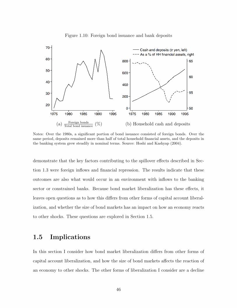
Figure 1.10: Foreign bond issuance and bank deposits

(a) Foreign bondsTotal bond issuance

(%) (b) Household cash and deposits

Notes: Over the 1980s, a significant portion of bond issuance consisted of foreign bonds. Over thesame period, deposits remained more than half of total household financial assets, and the deposits inthe banking system grew steadily in nominal terms. Source: Hoshi and Kashyap (2004).

demonstrate that the key factors contributing to the spillover effects described in Sec-

tion 1.3 were foreign inflows and financial repression. The results indicate that these

outcomes are also what would occur in an environment with inflows to the banking

sector or constrained banks. Because bond market liberalization has these effects, it

leaves open questions as to how this differs from other forms of capital account liberal-

ization, and whether the size of bond markets has an impact on how an economy reacts

to other shocks. These questions are explored in Section 1.5.

1.5 Implications

In this section I consider how bond market liberalization differs from other forms of

capital account liberalization, and how the size of bond markets affects the reaction of

an economy to other shocks. The other forms of liberalization I consider are a decline

46

in the risk free rate and changes in firm borrowing limits.

1.5.1 Decreasing the risk-free rate

One way in which capital account liberalization is often modeled is as a decline in the

risk free rate. For example, a closed economy with a high internal risk-free rate opens its

financial markets to abroad, and domestic agents can borrow more cheaply. To explore

how a fall in the risk-free rate compares to liberalization that occurs primarily in the

bond market, I consider four cases: an economy with banks only, an economy with only

bonds, an economy where all firms mix between bonds and bank debt, and a case in

which some firms borrow from banks and some firms mix. These cases demonstrate how

bonds amplify the effects of a decline in rf on interest rates, output, and productivity.

In an economy where the only option for financing is banks, the reduction in rf

passes through to the lending rate r, due to competition among banks.13 Declining

borrowing costs increase the incentives of firms to borrow. An increase in loan supply

is only possible if domestic banks are not constrained, an dif inflows provide additional

deposits for banks to intermediate. If banks are unconstrained, inflows lead to a decline

in r and an increase in output, until banks’ constraint binds, at which point r cannot

fall.

When there is only direct finance, a decline in rf makes financing cheaper for all

firms. Without banks, the lending rate equals the risk-free rate. A decline in rf

encourages marginal firms to take out loans. Inflows drive down the interest rate,

which discourages saving and encourages entry. This leads to a boom in output. As

in the bank-only case, because marginal entrants have lower productivity than the

existing group of active firms in the economy, productivity falls. However, the effect

of a decline in rf is larger relative to the bank-only case, because banks’ borrowing

13The extent of pass through observed empirically varies, see Harimohan et al. (2016), for example.

47

constraint provides an upper bound on inflows. Bond markets are not subject to such

frictions, and thus a decline in rf may lead to greater increases in output, relative to

the banks only case.

In an economy in which all firms issue bonds and also borrow from banks, i.e. f = 0

and m(a) > 0, there is a single participation threshold for borrowing that depends on

firm assets: z∗ = rf + m(a)θa

. A decline in rf leads to a decline in z∗, as well as a shift

in savings behavior. All firms can expand by borrowing more from bond markets, but

due to the minimum loan size requirement the entry threshold is lower for large than

for small firms.

When only a subset of firms issue bonds, the effect of a fall in rf on z∗ is negative, as

in the case above. When banks are unconstrained, the decline in rf does not affect the

size threshold for bond issuance a∗, which is a function of the spread r − rf . However,

when banks are constrained, the constraint limits the pass through of rf to r, and cause

a∗ to shift to the left. This implies more firms issue bonds. The shift in a∗ leads firms

to depend less on the banking sector, but amplifies the effect of the decline in rf among

firms large enough to issue bonds. As in the case of bond market liberalization, that

firms can access bond markets relaxes bank constraints, and allows banks to lend more

to small firms with marginal productivity.

The changes that result from a decline in rf are summarized in Proposition 1.3, and

shown graphically in Figure 1.11.

Proposition 1.3. Decline in the risk free rate. A decrease in rf :

1. weakly decreases a∗ (new issuers);

2. decreases z∗ (marginal large firms enter), provided f <∞;

3. decreases r (marginal small firms enter), by more for f ′ < f ;

4. increases Y (output), by more for f ′ < f ; and,

5. decreases Z (productivity), by more for f ′ < f .

48

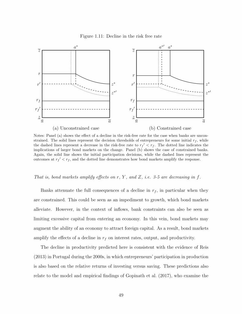
Figure 1.11: Decline in the risk free rate

az

z

a

r

z∗

a∗

r′

z∗′

rf

rf′

(a) Unconstrained case

az

z

a

r

z∗

a∗

r′

z∗′

a∗′

rf

rf′

(b) Constrained case

Notes: Panel (a) shows the effect of a decline in the risk-free rate for the case when banks are uncon-strained. The solid lines represent the decision thresholds of entrepreneurs for some initial rf , whilethe dashed lines represent a decrease in the risk-free rate to rf

′ < rf . The dotted line indicates theimplications of larger bond markets on the change. Panel (b) shows the case of constrained banks.Again, the solid line shows the initial participation decisions, while the dashed lines represent theoutcomes at rf

′ < rf , and the dotted line demonstrates how bond markets amplify the response.

That is, bond markets amplify effects on r, Y , and Z, i.e. 3-5 are decreasing in f .

Banks attenuate the full consequences of a decline in rf , in particular when they

are constrained. This could be seen as an impediment to growth, which bond markets

alleviate. However, in the context of inflows, bank constraints can also be seen as

limiting excessive capital from entering an economy. In this vein, bond markets may

augment the ability of an economy to attract foreign capital. As a result, bond markets

amplify the effects of a decline in rf on interest rates, output, and productivity.

The decline in productivity predicted here is consistent with the evidence of Reis

(2013) in Portugal during the 2000s, in which entrepreneurs’ participation in production

is also based on the relative returns of investing versus saving. These predictions also

relate to the model and empirical findings of Gopinath et al. (2017), who examine the

49

efficiency of capital allocation in Spain and Southern Europe following the adoption of

the Euro. The authors show increasing dispersion of the marginal revenue product of

capital within manufacturing industries, which is consistent with the broader range of

participation in production that results from a fall in the risk free rate in this framework.

Another common explanation for the real estate and stock market bubbles of the

1980s in Japan was the decline in interest rates, which fell from late 1980 until May

of 1989. Given the similarities between Propositions 1.2 and 1.3, the aggregate impli-

cations of a fall int eh risk free rate would go in the same direction as a bond market

liberalization, potentially amplifying the bond market’s effects.

1.5.2 Increasing firm borrowing

An increase in the parameter θ, which bounds the demand of firms for external fi-

nancing, increases firms’ borrowing. This can be interpreted either as an increase in

demand, a loosening of a binding firm borrowing constraint, or an increase in the col-

lateralizability of firm assets. In either case, the leverage firms can obtain is higher as

a result of the increase in θ.

Given a limited quantity of available funds, an increase in the demand for debt or

borrowing limits of individual firms allows higher productivity firms to reach a larger

scale, and crowds marginal borrowers out of the market for bank loans. To make clear

how the inclusion of bond markets affects the impact of an increase in firm borrowing

limits, I consider the same four cases as in the previous section: banks alone, bonds

alone, all firms mix, and some firms remain bank-dependent.

With bank debt alone and no bond market, banks’ borrowing constraints limit the

capital that banks can extend to firms. As a result, an increase in θ leads to an increase

in r, and marginal entrepreneurs no longer borrow and invest. A smaller subset of firms

obtain more funds, which is positive for both output and aggregate productivity. In the

50

case where banks are unconstrained, however, the increase in θ would have no impact

on r.

Without banks, if all projects are financed directly by household investment in

bonds, an increase in θ requires additional savings. Inflows fund the gap between new

demand and domestic savings, because there is no impediment to investment flowing

from abroad into bonds. There is no impact on r, and so the economy expands by more

than in the banks-only case. This increases productivity, because the scale of all active

firms increases.

When all firms mix between bank debt and bonds, an increase in θ can be met with

increased bond issuance. Bond markets provide a way around the bank constraint.

However, when some firms are bank-dependent, bond markets allow more large firms

to benefit from the increase in leverage, but small bank-dependent firms may be crowded

out. These effects are summarized in Proposition 1.4 and Figure 1.12.

Proposition 1.4. Increase in firms’ borrowing. An increase in θ:

1. decreases a∗ (new issuers);

2. decreases z∗ (marginal large firms enter), provided f <∞;

3. increases r (marginal small firms exit), by less for f ′ < f ;

4. increases Y (output), by more for f ′ < f ; and,

5. increases Z (productivity), by less for f ′ < f .

That is, bond markets amplify increases in Y , but attenuate changes in r and Z.

When banks have a limited capacity to intermediate funds, bond markets provide

an additional source of financing for firms. With banks alone, a rise in θ leads to an

improvement in the efficiency of capital allocation, as higher productivity firms are able

to produce more, and some marginal firms are crowded out of the borrowing market.

With bond markets, however, the effect on capital misallocation is less positive: given

51

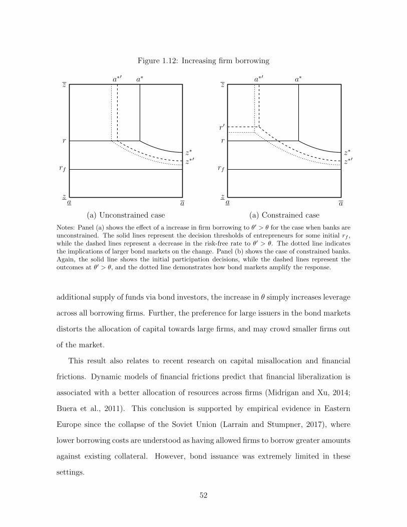
Figure 1.12: Increasing firm borrowing

az

z

a

r

z∗

a∗a∗′

z∗′rf

(a) Unconstrained case

az

z

a

r

z∗

a∗

r′

z∗′

a∗′

rf

(a) Constrained case

Notes: Panel (a) shows the effect of a increase in firm borrowing to θ′ > θ for the case when banks areunconstrained. The solid lines represent the decision thresholds of entrepreneurs for some initial rf ,while the dashed lines represent a decrease in the risk-free rate to θ′ > θ. The dotted line indicatesthe implications of larger bond markets on the change. Panel (b) shows the case of constrained banks.Again, the solid line shows the initial participation decisions, while the dashed lines represent theoutcomes at θ′ > θ, and the dotted line demonstrates how bond markets amplify the response.

additional supply of funds via bond investors, the increase in θ simply increases leverage

across all borrowing firms. Further, the preference for large issuers in the bond markets

distorts the allocation of capital towards large firms, and may crowd smaller firms out

of the market.

This result also relates to recent research on capital misallocation and financial

frictions. Dynamic models of financial frictions predict that financial liberalization is

associated with a better allocation of resources across firms (Midrigan and Xu, 2014;

Buera et al., 2011). This conclusion is supported by empirical evidence in Eastern

Europe since the collapse of the Soviet Union (Larrain and Stumpner, 2017), where

lower borrowing costs are understood as having allowed firms to borrow greater amounts

against existing collateral. However, bond issuance was extremely limited in these

settings.

52

The bond market liberalization in Japan was first designed to allow secured bond

issuance, followed by unsecured bond issuance later on. Arguably the former and

certainly the latter reform aimed to allow firms to issue debt beyond what they could

obtain in collateralized lending from banks. This could be interpreted as an increase

in θ. However, Japanese firms’ leverage was for the most part stable or falling during

the 1980s, so if anything this suggests that θ was declining. A decline in θ could also

put additional downwards pressure on lending rates, allowing more marginal firms to

borrow and produce, increasing output, but decreasing productivity.

The results of this section suggest that the growing influence of market-based fi-

nancing may affect future developments that affect demand for external finance or

allow firms to increase leverage. In both the Eastern and Southern European cases,

banks received considerable inflows, which is evidence that a constraint on banks was

far from binding, at least in the early 2000s. This changed dramatically after 2008,

when many banks faced serious difficulties, either due to their own loan portfolios and

the economic downturn, or through exposures to troubled sovereigns. The effects of

such bank shocks are explored in the next section.

1.5.3 Bank shocks

The availability of substitutable forms of finance is understood to dampen the impact

of bank shocks, and yet such shocks still played a significant role in the fall in output

post-2008 (e.g., Chodorow-Reich, 2014). Similarly, banks in Japan suffered a large

shock following the collapse of land prices and the stock market bubble in the early

1990s. Gan (2007b) estimates the effect of the collapse of land prices on bank lending,

using variation in banks’ exposure to real estate, including land holdings.

In the model presented here, a shock of this nature corresponds to a decline in either

banks’ borrowing constraint φ or bank equity E. If banks are unconstrained such a

53

shock has no effect, as shown in panel (a) of Figure 1.13. For constrained banks, the

effects are explored in Proposition 1.5.

Proposition 1.5. Decrease in banks’ borrowing capacity. When D = φE, a decrease

in φ or E:

1. decreases a∗ (new issuers);

2. does not change z∗ (no change for large firms);

3. increases r (marginal small firms exit), by less for f ′ < f ;

4. decreases Y (output), by less for f ′ < f ; and,

5. increases Z (productivity), by less for f ′ < f .

That is, bond markets attenuate the increases in r and Z, and the decreases in Y .

A shock to bank borrowing φ or bank equity E causes the deposit demand of the

financial sector to fall. The fall in loan supply leads to an increase in r. When loans are

more expensive, fewer firms borrow, and more firms issue bonds (i.e. a∗ falls), as shown

in panel (b) of Figure 1.13. Output contracts and productivity improves, because firms

that continue to have access to external finance are more productive than firms that can

no longer borrow. The increase in r increases bank profits, and decreases entrepreneurs’

profits.

Bond markets cushion the impact of the initial shock on interest rates: as r rises,

more firms issue bonds instead of bank debt, which allows for more production than if

banks were to intermediate capital alone. Bond markets thus attenuate the decline in

output. To see this, consider an economy without bonds. A shock to bank equity leads

to a decline in loan supply. For the lending market to clear, a large increase in r is

necessary. The savings that banks cannot intermediate because of the bank borrowing

constraint flow abroad. With bond markets, the increase in r not only discourages

borrowing from banks, but also makes issuing bonds more attractive. Some savings

54

Figure 1.13: Bank shocks

az

z

a

r

z∗

a∗

rf

(a) Unconstrained case

az

z

a

r

z∗

a∗

r′

a∗′

rf

(b) Constrained case

Panel (a) shows the effect of a tightening of bank borrowing limits φ′ < φ for the case when banks areunconstrained. When banks’ constraint does not bind, this has no effect. Panel (b) shows the caseof constrained banks. Here, the solid line shows the initial participation decisions, while the dashedlines represent the outcomes at φ′ < φ, and the dotted line demonstrates how a larger bond marketsfurther dampens the effects of the shock.

can move from bank deposits to investing in bonds. As a result, r increases by less,

relative to the case in which there is no direct finance.

In dampening the effects of a financial shock on the economy, however, bond markets

also slow the pace of bank recovery. At a lower r, bank profits are lower. Consequently,

there is slower growth in bank net worth. This has implications for policies that en-

courage bond issuance. For example, in reducing bond yields, quantitative easing may

limit the prospects for bank recovery.

Japan’s bond market liberalization seemed like a positive liquidity shock for banks.

However, a different perspective is that the loss of large, highly profitable borrowers

negatively impacted banks’ long-run franchise value. The collapse of the asset price

bubble affected the operations of banks that had increasingly lent to real estate com-

panies. The real estate companies held assets that had grown enormously in value and

55

were a common form of loan collateral. Later, banks evergreened loans to avoid losses

to bank equity. As higher capital requirements were introduced in the 1990s, banks

acted to avoid shocks to their net worth that would require contemporaneous decreases

in the sizes of their lending portfolios. Ultimately, the consolidation and contraction

necessary among Japanese financial institutions is a problem that continues to have

implications today.

1.6 Conclusion

This chapter revisits the bond market liberalization in the 1980s in Japan as a case

that highlights the interactions between bond markets and banks. I demonstrate that

the liberalization led firms to issue bonds that were primarily used to repay bank debt.

The repayment of bank debt was a positive liquidity shock for banks that lent to firms

affected by the liberalization shock. This liquidity shock was transmitted by banks to

firms in other parts of the economy, namely bank dependent firms, small and medium

firms and real estate companies. This expansion in bank activity led to increased bank

exposure to riskier segments of the economy.

I develop a model to make sense of the empirical evidence, in which firms borrow

from banks and issue bonds. The model matches the empirical evidence and demon-

strates that the key factors that led the bond market liberalization to have spillover

effects via banks were the repression of domestic savers, combined with foreign invest-

ment in the bond market. This in particular contributed to excess deposits at banks,

which then drove lending to marginal borrowers in the economy. The Japanese case is

in this respect similar to other liberalization episodes. However, the channel by which

inflows affected Japan differed, by flowing through corporate borrowers and indirectly

reaching banks and other firms.

The transition to greater market-based financing is also relevant in other markets.

56

China has successfully established a large and fast-growing corporate bond market over

the past decade. Despite increased offshore issuance in recent years, foreign investment

in Chinese bond markets remains limited. However, new programs introduced to allow

foreign investors to buy onshore bonds via the Hong Kong bond market are estimated

to spark inflows of up to US$ 250 million by 2020.14 China’s inclusion in emerging-

market bond indices is likely to encourage further foreign investment in Chinese bonds.

The model and results presented here suggest policymakers should be wary of how this

impacts Chinese lenders.

In developed markets also, the importance of bond markets has grown steadily in

recent years, encouraged by both the slow post-crisis recoveries of many banks and

policies that facilitate bond issuance and/or reduce bond yields. The evidence in this

chapter suggests that this will affect not only bank outcomes but also the reaction of

economies to future shocks. In particular, bond markets appear to amplify positive

shocks such as increases in firm borrowing and declines in the risk-free rate, while

attenuating the impact of negative financial shocks. In relaxing banks borrowing con-

straints, bond markets surge both in booms, and when there are financial crises. These

results suggest that characterizing bond markets and these asymmetries is important to

refining the approaches that incorporate financial frictions in macroeconomic models.

14”The Economist, “Financial assets, made in China.” June 22, 2017.

57

Chapter 2

Default, commitment, and domestic

bank holdings of sovereign debt

2.1 Introduction

Financial institutions generally hold large amounts of sovereign debt, and, in particular,

the debt of their own sovereign. A recent literature has documented this globally

(Gennaioli et al., 2014a), and specifically in the context of the European sovereign debt

crisis (Broner et al., 2014; Brutti and Saure, 2014). In turn, a growing literature has

explored the implications of these holdings for sovereign default, noting that the ability

of foreigners to sell their bonds to domestic investors makes selective defaults difficult

(Broner et al., 2010), emphasizing that with large bank holdings, sovereign default leads

to contractions in credit and output losses (Gennaioli et al., 2014b; Perez, 2015), and

arguing that financial repression may explain some of these holdings, and that such

policies may be motivated by generating a commitment to not default (Becker and

Ivashina, 2014; Chari et al., 2015).

This chapter provides a three-period model to further explore how domestic bank

holdings of sovereign debt interact with sovereign default and financial repression. In

particular, I provide a joint answer to the following three questions: How do domestic

banks affect the default incentives of the sovereign? Second, how does sovereign risk

58

affect domestic demand for government debt? Third, how do these holdings affect

government policy towards banks, and in particular, financial repression?

The model has two central ingredients and a series of predictions that follow from

them. First, banks demand government debt because it serves as collateral in interbank

markets, which is valuable for liquidity management, modeled as banks being matched

with investment projects that exceed what they collect as deposits. This use of gov-

ernment debt is emphasized by Bolton and Jeanne (2011) and Gorton and Ordonez

(2013). It implies that banks’ demand for government bonds is downward-sloping, and

depends on the extent of liquidity needs as well as on the expected return on the bond.

Banks with access to investment opportunities choose to invest in government debt

in order to collateralize interbank lending. Without access to alternative safe assets,

higher sovereign risk may increase demand for sovereign debt because banks require

government assets to pledge as collateral.

Second, banks are a crucial source of credit to firms. However, banks are constrained

in their lending by the amount of equity they hold. Financial frictions in the form of

an agency problem on bankers that can divert funds puts a limit on banks’ ability

to attract deposits. When there is a default on government bonds, bank equity falls,

which reduces the ability of banks to attract deposits. This in turn limits the bank

funding available to the real economy and leads to declines in output. These endogenous

output losses provide a commitment technology to sovereigns, and default costs increase

with domestic banks’ holdings of government debt. This also provides a microfounded

explanation for the secondary market theory of Broner et al. (2010), demonstrating one

way in which bonds are more valuable in the hands of domestic agents.

As in any canonical model of sovereign default, the probability of default is increas-

ing in the amount of foreign borrowing and there is a Laffer curse on the total amount of

resources borrowed from abroad. However, the output losses from default in this model

59

are endogenous. Because the output losses are endogenous, the model can generate

positive holdings of risky debt and default in equilibrium. Moreover, the model makes

the surprising prediction that default is more likely when banks are well-capitalized. In

the model, there can be deposit flight both in anticipation of and as a consequence of

default, and higher levels of initial deposits are shown to lead to lower default risk.

Like in Gennaioli et al. (2014b) and Perez (2015), sovereign defaults are followed

by large contractions in private credit, and default has more severe effects but is less

likely when banks hold more public debt. Unlike these authors, banks demand public

debt to use as collateral, instead of as a store of liquidity. Relative to Perez (2015),

this chapter assumes that banks with investment opportunities have a motive to hold

government bonds, and that default disrupts deposits. In contrast to Gennaioli et al.

(2014b), lending to public and private projects is contemporaneous, the return on both

is uncertain, and the probability of default is determined endogenously as a function of

the realized level of private productivity.

In addition, banks choose how many bonds to hold to maximize profits, but the

government chooses to default to maximize social welfare. Because domestic banks

take bond prices and default probabilities as given, yet their holdings of bonds affect

the incentives of the policymaker to default, there is a pecuniary externality. Financial

repression can increase welfare, since the competitive equilibrium leads to under-holding

of government bonds. However, financial repression can seldom prevent default entirely,

and in the event of default leads banks and households to be strictly worse off.

The rest of the chapter is structured as follows. The remainder of this section re-

views related literature. In Section 2.2, I present the model and define equilibrium.

The results of the model are described in Section 2.3. Section 2.4 explores the external-

ity that arises from domestic holdings of sovereign debt, and discusses the optimality

of financial repression. In Section 2.5, I discuss two extensions of the model, which

60

incorporate a second safe asset, and foreign capital inflows to banks. The final section

concludes.

2.1.1 Related literature

This chapter relates to research on sovereign default, financial frictions, and bank hold-

ings of government debt.

There is a considerable literature in economics focused on sovereign default.1 Canon-

ical sovereign default models (Eaton and Gersovitz, 1981; Arellano, 2008) consider ex-

clusion from financial markets and exogenously assumed output losses to discipline

borrowers. That sovereign crises are often coincident with banking crises is shown by

Reinhart and Rogoff (2008).2 Gennaioli et al. (2014b) model banks that lend to the

government as a store of liquidity, and can then make fewer private investments in the

event of nonrepayment. They also provide empirical evidence that banks’ sovereign ex-

posures are associated with post-default declines in credit. The current chapter instead

models a contemporaneous choice between public and private investment, and assumes

public debt is necessary to collateralize interbank lending. In addition, in this chapter

the productivity of private investment is subject to uncertainty, and its realization af-

fects bank and household income, which leads default to be a function of the realization

of productivity as well as other parameters in the model. This characterization allows

further scrutiny of the interaction between government and bank incentives.

A number of papers provide quantitative assessments of the link between government

debt, domestic banks, and the real economy. Sosa Padilla (2015) provides a quantitative

closed-economy model in which banks lend to the government and firms, and firms

1For surveys, see Eaton and Fernandez (1995) and Aguiar and Amador (2014).

2A number of authors note that this link has been particularly important in the evolving Europeancrises, for example, Angeloni and Wolff (2012), Popov and van Horen (2013), and Brunnermeier et al.(2011).

61

require external financing to pay workers up front. Other authors focus on identifying

the balance sheet channel in addition to other effects: Bocola (2015) incorporates a risk

channel by which banks lend less to a worsening economy, with exogenous default, and

Perez (2015) considers the reduced value of public debt as liquidity, with endogenous

default. In contrast, the main mechanism by which bank losses occur in this chapter

are via deposits, which shrink in anticipation and as a consequence of default.

In addition to the costs of exclusion and bank losses, well-functioning secondary

markets can help support risky sovereign debt. Broner et al. (2010) argue that if do-

mestic bondholders are relatively more capable of extracting value from a sovereign

following a default, or if the sovereign is less likely to default on them, then in antici-

pation of a default foreigners sell their debts to domestic agents via secondary markets.

As a result, it is difficult for governments to default selectively on foreigners. I show

that secondary market theory has an additional underlying driver, in the commitment

value of domestic creditors. In this model, domestic creditors affect the repayment

incentives of debt in a way that better supports the value of debt, which produces a

similar outcome as the political economy explanation that domestic agents are more

likely to receive compensation from the government after a default.

Although I do not model secondary markets explicitly, I assume that the sovereign

is unable to default selectively on foreign lenders. Sturzenegger and Zettelmeyer (2008)

document empirically that following a sovereign default, both domestic and foreign

creditors suffer losses. Erce (2012) explores historical patterns of selective default, and

finds that it is more common for governments to default on domestic creditors when

the banks are not weak, a key prediction of my model.

In addition, I draw from a large literature on the impact of credit disruptions on the

real economy. Much research has shown how financial frictions can worsen an economic

slump (Bernanke and Gertler, 1989; Bernanke et al., 1999). I adopt financial frictions

62

following the form of Gertler and Kiyotaki (2010), and expand the role of government

to allow for sovereign default.3 This provides a simple microfoundation for the credit

disruption that occurs when a sovereign defaults on domestic banks.

There is also a large body of research that considers what motivates bank port-

folios of sovereign debt. In advanced economies, many financial intermediaries use

sovereign assets for risk and liquidity management purposes. In developing countries,

bank holdings of government bonds may also be driven by a lack of alternatives due

to the relatively underdeveloped nature of financial systems (Woodford, 1990; Holm-

strom and Tirole, 1998; Kumhof and Tanner, 2008). Given that government debt often

has a nearly “risk-free” status, banks use government debt as collateral for interbank

loans or repos (Bolton and Jeanne, 2011). Based on this idea, I model banks requiring

government debt for use as collateral in interbank markets. Sovereign debt is also used

to access to public liquidity: banks can often access cheap lending from central banks

collateralized by government debt and other highly rated securities.

As for why banks demand debt of their own sovereign specifically, a number of

theories complement the explanations above. Standard theories of portfolio allocation

and home bias have some portion of each bank’s portfolio held domestically. Financial

repression consists of governments forcing banks to hold sovereign debt or using “moral

suasion,” to compel them to do so, and has been a prominent explanation both histor-

ically and in present times (Reinhart et al., 2003; Reinhart, 2012; Becker and Ivashina,

2014). In addition, governments may provide incentives for banks to hold domestic

sovereign bonds. For example, in Europe, EU government debt receives a zero percent

risk weight on the balance sheets of European banks, and is exempt from limits on

large exposures.

Finally, this chapter relates to a growing body of empirical research on the shifting

3An additional reference for Gertler and Kiyotaki (2010) are teaching notes by Christiano and Zha(2010) and Groth (2011), who demonstrate a two-period version of the model.

63

patterns of sovereign debt ownership in current-day Europe. The height of the European

debt crisis coincided with the beginning of a large-scale “repatriation” of sovereign

debt holdings, particularly in Greece, Ireland, Italy, Portugal, and Spain (GIIPS). The

percentage of debt held by domestic creditors in these countries increased since the mid-

2000s, and rose dramatically around the height of the crisis. A number of explanations

for this have been put forth: secondary market theory (Broner et al., 2014; Brutti and

Saure, 2014), financial repression (Becker and Ivashina, 2014), ECB policy (Crosignani

et al., 2015), and reaching for yield (Acharya and Steffen, 2015). This model provides a

framework for thinking about risky sovereign debt that is owed both domestically and

abroad, and how domestic holdings and default incentives interact.

2.2 Model

The model combines a canonical model of sovereign default with Gertler and Kiyotaki

(2010) style financial frictions, to characterize the interaction between foreign lenders,

government default and domestic banks. This is introduced using a three period setup,

where the government can borrow only in t = 0 debt that is due in t = 1. By using this

framework, I abstract from the potential for exclusion from foreign financial markets,

to characterize more sharply the role of domestic banks and endogenous output losses.

2.2.1 Setup

The timing of the model is as follows:

• In t = 0, the government borrows from foreign lenders and domestic banks to

invest in a public project of fixed size g. Households begin with an initial endow-

ment that they can consume or save at banks. Banks lend to the government, to

64

other banks, and to firms. Foreign investors lend to the government. The real-

ization of underlying productivity A1 is uncertain at t = 0, for some A1 ∈ [A,A].

• In t = 1, the productivity level A1 of the economy is realized, and firms produce.

Given A1, the government decides whether to repay its debt or default. Default

leads to financial frictions in the form of an incentive constraint on domestic

banks. Households consume and save, and bankers lend to firms.

• In t = 2, firms produce, and banks shut down and return their net worth to

households, who consume.

The detailed optimization problem of each group of agents is described below.

2.2.2 Households

Households are assumed to be risk-neutral savers who care equally about all three

periods, and choose consumption to maximize:

c0 + E [c1 + c2] , (2.1)

subject to the budget constraints:

c0 + d0 = y0,

c1 + d1 = R1d0 − btot · I{D=0}, (2.2)

c2 = R2d1 + n2. (2.3)

Households receive an initial endowment y0, earn gross interest rates of R1 and R2 on

intertemporal deposits d1 and d2, and are assumed to receive a transfer of the equity

remaining in banks n2 at t = 2. If the government does not default, denoted by D = 0,

then households pay taxes in order to repay the country’s total debt btot.

65

2.2.3 Government

The government’s optimal program satisfies:

V0 = maxbtot

[c0 + E

[maxD∈{0,1}

{V1, Vd

1 }]], (2.4)

where D denotes the government’s default decision, and the government is assumed to

choose foreign borrowing b∗ to meet a fixed exogenous level of public spending:

g = qbtot,

where q is the price. Of the total debt issued by the government, some portion b will be

held by domestic banks, and the remainder b∗ is assumed to be held by foreign lenders:

btot = b+ b∗.

The continuation values in period 1 are given by:

V1(b, b∗, A1) = c1 + c2,

V d1 (b, b∗, A1) = cd1 + cd2,

where ct and cdt denote consumption conditional on no default and default, respectively,

and A1 ∈ [A,A] is the stochastic realization of private productivity in t = 1.

The default set is defined as the set of realizations for which default is optimal,

given b and b∗:

∆(b, b∗) = {A1 ∈ A : V1 < V d1 }.

Default probabilities and default sets are related in the following way:

p(b, b∗) =

∫∆(b,b∗)

f(A)dA, (2.5)

where f(·) is a probability density function for the realizations of A1.

66

2.2.4 Foreign lenders

Foreign lenders are assumed to be risk neutral and to lend at an interest rate that

compensates them for default risk, maximizing profits in each period. Their opportunity

cost is assumed to be the gross risk-free rate, R, yielding profits:

φ = qb∗ − 1− p(b, b∗)R

b∗.

In what follows, it is assumed that the government issues enough debt that both do-

mestic and foreign lenders hold bonds, and the price of government debt is accordingly:

q =1− p(b, b∗)

R, (2.6)

where q takes values on a bounded interval q ∈[0, 1

R

].

2.2.5 Banks

Banks begin with initial equity n0 and accept deposits d0 from households. The main

mechanisms of the model arise from two financial frictions: interbank lending that must

be collateralized, and an agency problem in deposit markets. I describe each of these

in turn.

Collateralized interbank lending

Following Bolton and Jeanne (2011), I assume that banks have heterogeneous access

to investment projects, but demand deposits homogeneously.

Specifically, at t = 0, a fraction ω of banks get access to the production technology,

while 1−ω do not. Banks with projects demand domestic government debt in order to

be able to borrow on interbank markets. The size of interbank loans is limited by the

value of collateral. Eligible securities are in this case only government bonds, which

67

are assumed to be collateralized with some haircut λ ≥ 1.4 Banks holding government

debt of qb can borrow up to a limit:

i ≤ λqb.

Banks are assumed to act competitively in the market for sovereign debt, i.e., taking

the price q as given. Government debt is first assumed to be the only asset that can be

used to collateralize interbank loans, an assumption that is relaxed in Section 5.

Equity and deposits form the liabilities side of banks’ balance sheets, and can be

invested in government bonds qb or lent to firms k1. I also allow banks to invest excess

funds in a risk-free asset that pays R, and denote excess funds by x. The balance sheets

of banks with and without investment projects are shown in Figure 2.1.

Banks with projects Without projects

Assets Liabilities Assets Liabilitiesk1 ω d0 i (1− ω)d0

qb ω n0 x1 (1− ω)n0

i

Figure 2.1: Heterogeneous bank balance sheets

The rate paid on interbank lending is assumed to equal the overall return earned

on private investment and government debt. This makes depositors indifferent be-

tween banks with and without investment projects, and allows banks to be treated as

homogenous, in aggregate.

At t = 0, banks without investment projects have (1−ω)(n0 + d0) of liabilities that

can only be productively invested in interbank markets, government bonds, or the risk

4In general, λ ≥ 1, because for lower values of the haircut domestic banks are able to borrow lessthan one dollar on interbank markets for each dollar they lend to the government. If λ < 1, banks arebetter off not lending to the sovereign at all.

68

free asset. This places a constraint on the supply of interbank funds:

i ≤ (1− ω)(n0 + d0).

In equilibrium, banks with projects invest in government debt; banks without

projects make collateralized loans to banks with projects.

For a given q, banks with projects demand a sufficient level of government debt

to borrow all the funds at banks without investment projects. This assumes that the

resources held by productive banks is larger than (1 − ω)(n0 + d0)/λ. This leads to

domestic demand for government debt of:

bopt =(1− ω)(n0 + d0)

λq, (2.7)

which allows all funds in the economy to be intermediated. If the government issues

less debt than the amount in equation (2.7), the lack of collateral hinders interbank

lending and leads to efficiency losses. For a given b, the amounts of interbank lending

and remaining excess funds are given by:

i = min

{b

bopt, 1

}(1− ω)(n0 + d0),

x = max

{1− b

bopt, 0

}(1− ω)(n0 + d0). (2.8)

In what follows I focus on cases in which btot > bopt.

In the three-period model, sovereign debt and interbank markets are only open

once, from t = 0 to t = 1. At t = 1, all banks are assumed to have equal access to

investment projects (as there is no longer a market for government debt, and therefore

no collateral).

If b ≥ bopt, the balance sheet constraints of the aggregate banking system are:

k1 + qb = n0 + d0, (2.9)

k2 = n1 + d1. (2.10)

69

Banks choose government debt holdings, lending to firms, and deposits to maximize

expected equity in t = 2:

E [n2] , (2.11)

where equity evolves according to:

n1 = A1k1 + b · I{D=0} −R1d0, (2.12)

n2 = A2k2 −R2d1. (2.13)

For banks that have access to the production technology, investment capital yields

constant returns to scale, where A1 is stochastic, but A2 is fixed. If the government

defaults, banks suffer a loss to equity relative to the no default case.

So that households are not insulated from the productivity realization in the econ-

omy, I assume that the interest rate on deposits in period 1 is state-contingent, i.e. the

interest rate on deposits is given by:

R1 = A1.

While many countries insure deposits, this characterization of the return on deposits is

helpful in that it exposes both banks and depositors to the realization of productivity

in the economy. If R1 were fixed, this would allow banks to become very rich when

the realization of productivity is high, but cause them to have outsized losses when the

realization of productivity is low. Similarly, if there are no financial frictions in t = 1:

R2 = A2.

These assumptions also ensure that banks do not end up with negative equity. Although

the possibility of bank failures is not considered explicitly in the model, this would likely

worsen the consequences of default.

70

Deposit market frictions

Financial frictions are assumed to arise in interbank markets when bank equity is low,

so that depositors are concerned about the health of banks. Following Gertler and

Kiyotaki (2010), this is modeled as an agency problem in that bankers are capable of

diverting a fraction θ of bank assets. This adds an incentive constraint to the banks’

problem: the profits of operations must be greater than the value of assets bankers

can divert. In the case that financial frictions arise as a consequence of default, this

incentive constraint can be written as:

A2k2 −R2d1 ≥ θA2k2. (2.14)

Using equation (2.10), the constraint can also be written as a condition on deposits:

d1 ≤(1− θ)A2

R2 − (1− θ)A2

n1. (2.15)

This inequality can only hold if R2 > (1 − θ)A2. Bankers’ demand for funds is thus a

well-defined function of R2 in the interval ((1−θ)A2, A2], and decreasing in R2. Deposit

demand approaches infinity as R2 → (1 − θ)A2, and approaches 1−θθn1 as R2 → A2.

When R2 = A2, deposit demand is bounded:

0 ≤ d1 ≤1− θθ

n1.

The deposit demand of banks in the case of financial frictions therefore follows:

ddemand1 =

(1−θ)A2

R2−(1−θ)A2n1 if R2 < A2

Indeterminate in [0, 1−θθn1] if R2 = A2

0 if R2 > A2

.

With risk neutral households that care equally about each period, any interest rate

71

greater than 1 will induce them to save everything, so deposit supply follows:

dsupply1 =

R1d0 if R2 > 1

Indeterminate in [0, R1d0] if R2 = 1

0 otherwise

.

This can be combined with the bound d1 ≤ 1−θθn1 to solve for the bound on bank equity

below which financial frictions arise:

n1 ≥θ

1− θR1d0 = N . (2.16)

Combining deposit demand and deposit supply results in equilibrium in the deposit

market, which pins down both d1 and R2. For any shock that causes bank equity to

decrease below the threshold in (2.16), banks continue to operate but are subject to an

additional incentive constraint given by equation (2.14). For equation (2.14) to hold,

either the return on deposits must fall, or the amount of deposits must fall, or both.

In this way, a government default causes stress in the banking system, and generates

an endogenous cost of default.

In the event of default, households have more wealth because they do not pay taxes

to repay debt, as in equation (2.2). Because the households are wealthier, for deposits

in the economy to fall, rather than rise, it must be that the savings that are deposited

under financial frictions in equation (2.15) are less than deposits if there is no default:

(1−θ)A2

R2−(1−θ)A2nd1 < R1d0 − btot. If the equilibrium in deposit markets is such that the level

of deposits is less than the frictionless level, it can only be that the deposit demand

condition intersects deposit supply on the vertical line where R2 = 1. This is shown

graphically in Figure 2.2.

72

d

(1− θ)A

d

1−θθn

A

ddemand

1

dsupply

Figure 2.2: For deposits to fall after default, assuming nd1 < N

2.2.6 Equilibrium

Equilibrium in this economy consists of the government maximizing welfare, households

maximizing expected utility, banks and foreign investors maximizing expected profits,

and market clearing for deposits, interbank lending, and sovereign debt.

Definition 2.1. Equilibrium in this economy is defined as a set of policy functions for

consumption {c0, c1, c2}, deposits {d0, d1}, lending {k1, k2}, government asset holdings

{b, b∗}, default sets ∆(b, b∗) and bond prices q(b, b∗) such that:

1. Taking as given government policies and bond prices, consumption and deposit

supply plans {c0, c1, c2} and {d0, d1} maximize households’ expected utility subject

to their budget constraints.

2. Taking as given government policies and bond prices, banks choose deposits and

lending to the government and firms to maximize expected equity E [n2], subject to

balance sheet constraints, the evolution of net worth, and an incentive constraint

that occasionally binds; and, interbank markets clear.

3. Deposit markets clear, meaning that deposit demand and supply from the banks’

and households’ programs determine the level of deposits and the deposit rate.

73

4. Taking as given bond prices, the government’s asset holdings b and b∗, and default

sets ∆(b, b∗) satisfy the government’s optimization problem.

5. Bond prices q(b, b∗) reflect the government’s default probabilities and are consis-

tent with foreign lenders’ expected zero profits.

The model can be solved backwards, by first determining the solutions to the prob-

lem at t = 1. Since there is no uncertainty after A1 is realized, it is possible to compare

V1 and V d1 for given levels of b, b∗, and realizations of A1 to determine when default will

be optimal. These solutions can be then be considered in t = 0 along with an assumed

probability distribution for the possible realizations of A1, to determine the optimal b

and b∗.

2.3 Results

This section characterizes the equilibrium outcomes in the model. First, domestic debt

is shown to be a commitment device. Second, the implications of domestic banks’ char-

acteristics for sovereign default are explored: default is more likely on well-capitalized

banks, and default risk decreases with the level of bank deposits. Next, because the

usefulness of debt as collateral is tied to its value, domestic demand for sovereign debt

increases with default risk. Two features of canonical sovereign default model remain

true in this setup: default incentives increase in the level of foreign lending, and default

occurs in equilibrium. Finally, the model is used to show that financial frictions and

deposit flight in anticipation of default are likely to increase the costs of default, while

also making default more likely.

Three basic properties of the model are first discussed, before turning to the main

results. For the model to generate interesting predictions, one additional restriction is

74

necessary. Banks are assumed to have only a limited amount of equity, which can be

stated as a condition on model parameters.

Assumption 2.1. Initial bank equity is assumed to be lower than the threshold:

n0 < d0

[1

A2(1− θ)λ

λ+ ω − 1− 1

].

Assumption 2.1 guarantees that default occurs when productivity is low.5 However,

in the absence of domestic bond holdings, there is no cost to default. In equilibrium,

domestic holdings of sovereign debt must be large enough that a default results in

financial frictions in order for there to be any cost associated with non-repayment.

Lemma 2.1. Domestic bond holdings must be (i) strictly positive and (ii) sufficiently

high so that a default results in financial frictions, in order for foreign lending to be

supportable in equilibrium.

Proof. All proofs are included in the Appendix.

In this three period setup, there is no threat of exclusion from financial markets to

discipline government borrowers. If the government has no borrowings from domestic

banks, then for any positive value of foreign lending default is certain. Therefore, no

lending can be supported in equilibrium. Similarly, for a level of borrowing too small

to cause distortions in the domestic banking sector, there is no cost to defaulting to

encourage the government to repay. However, to the extent that domestic holdings of

sovereign debt can disrupt the banking sector and become a source of output losses in

the event of default, foreign lending can be supported in equilibrium.

If domestic banks are the only holders of sovereign debt, then default is trivial,

because it generates output losses as a result of financial frictions, without providing

5The condition in Assumption 2.1 is derived in the proof of Lemma 3.

75

any benefits from retaining resources that would otherwise be transferred abroad. This

is demonstrated in the following Lemma, which considers the case where foreigners hold

no debt, i.e. b∗ = 0.

Lemma 2.2. If b > 0 and b∗ = 0, then ∆(b, b∗) = ∅, i.e., when all sovereign debt is

held by domestic banks, default is never optimal.

The government default decision involves a tradeoff between the benefit of lower

lump-sum taxes, and the costs of default on the banking system. A default exclusively

on domestic bondholders is never optimal, since this comes with costs and has no

associated benefits. Default merely causes a redistribution of wealth from banks to

households. Households then cannot save as much at impaired banks, and investment

and output fall. Since taxation is lump sum and bank equity is returned to households

in t = 2, this makes households worse off.

Models of non-contingent sovereign debt typically find that defaults occur when

output is low. Given Assumption 2.1, this is also true in this model, and there is some

threshold value of A1 below which default is optimal.

Lemma 2.3. If for a level of borrowing (b, b∗) default is optimal for some A1, then

default is also optimal for all A′1 < A1. Therefore, there exists a threshold level of

productivity A ∈ [A,A] below which it is optimal for the government to default.

It follows from Lemma 2.3 that for each level of domestic and foreign debt, the set

of productivity realizations that trigger default is an interval. This simplifies solving

the model, because the default probability in equation (2.5) can be rewritten as:

p(b, b∗) = F (A),

where F (A) =∫ AAf(A)dA is the cumulative distribution function of the possible real-

izations of productivity A1. By extension, agents’ expectations can be written as the

sum of two integrals, taken over the default and no default regions of [A,A].

76

AA

V1

V d1

Figure 2.3: Threshold level of A1

2.3.1 Commitment

Taken together, Lemmas 2.1-2.3 demonstrate the importance of domestic bond holders

in contributing to the commitment of a sovereign in repaying its debts, through the

endogenous costs of default. This result is stated formally in Proposition 1.

Proposition 2.1. For b < b′, ∆(b′, b∗) ⊆ ∆(b, b∗), i.e. the default set is decreasing in

the amount of domestically held sovereign debt.

In the model, the government can borrow from abroad because defaulting leads

to financial frictions that limit the ability of banks to channel savings to productive

investment. Greater domestic holdings of sovereign debt lead to more severe effects on

the banking system in the event of default, which lowers default risk. This is the only

effect which serves to discourage default in this model. In reality, other disciplining

devices play a role as well, such as exclusion, reputation, secondary markets, etc.

From the perspective of the government issuer, domestic holders are distinct because

their bond holdings come with additional associated losses if the sovereign defaults.

This helps to support the value of sovereign debt, by raising the price q, or equivalently

lowering the default probability p. In this sense, a bond in the hands of domestic

77

investors is more valuable due the effect that endogenous output losses have on default

incentives.

Importantly, this property of domestic bond holders provides a microfoundation for

the assumption in secondary market theory that domestic shareholders place relatively

more value on government debt in times of sovereign stress. This can be framed in terms

of political economy explanations, such as that domestic creditors are more likely to

be able to extract value from the government following a default, perhaps because

domestic bond holders are more concentrated and have more sway in domestic political

processes. However, the same conclusion - that there is more value to debt in the

hands of domestic creditors - emerges from the framework of this model, driven by

commitment. Domestic creditors support the value of sovereign debt precisely because

defaulting on them is costly.

2.3.2 Bank health

An extension of the idea of domestic banks as a commitment device is how default

incentives depend on characteristics of the banking system. A well-capitalized banking

system is more easily able to weather a sovereign default. In contrast, fragile banks are

more costly for the sovereign to default on. This is the intuition of Proposition 2.2.

Proposition 2.2. Holding constant the level of foreign debt, ∆(b, b∗) is increasing in

n0, i.e. default is more likely if banks have more equity.

In the event of default, financial frictions limit bank deposits to some multiple of

bank equity. When initial bank equity is low, a default leads to a tighter constraint

on deposits, which leads to a higher cost of default. In comparison, a well-capitalized

banking system is less constrained in the event of default, leading default to be less

costly, and therefore more probable.

78

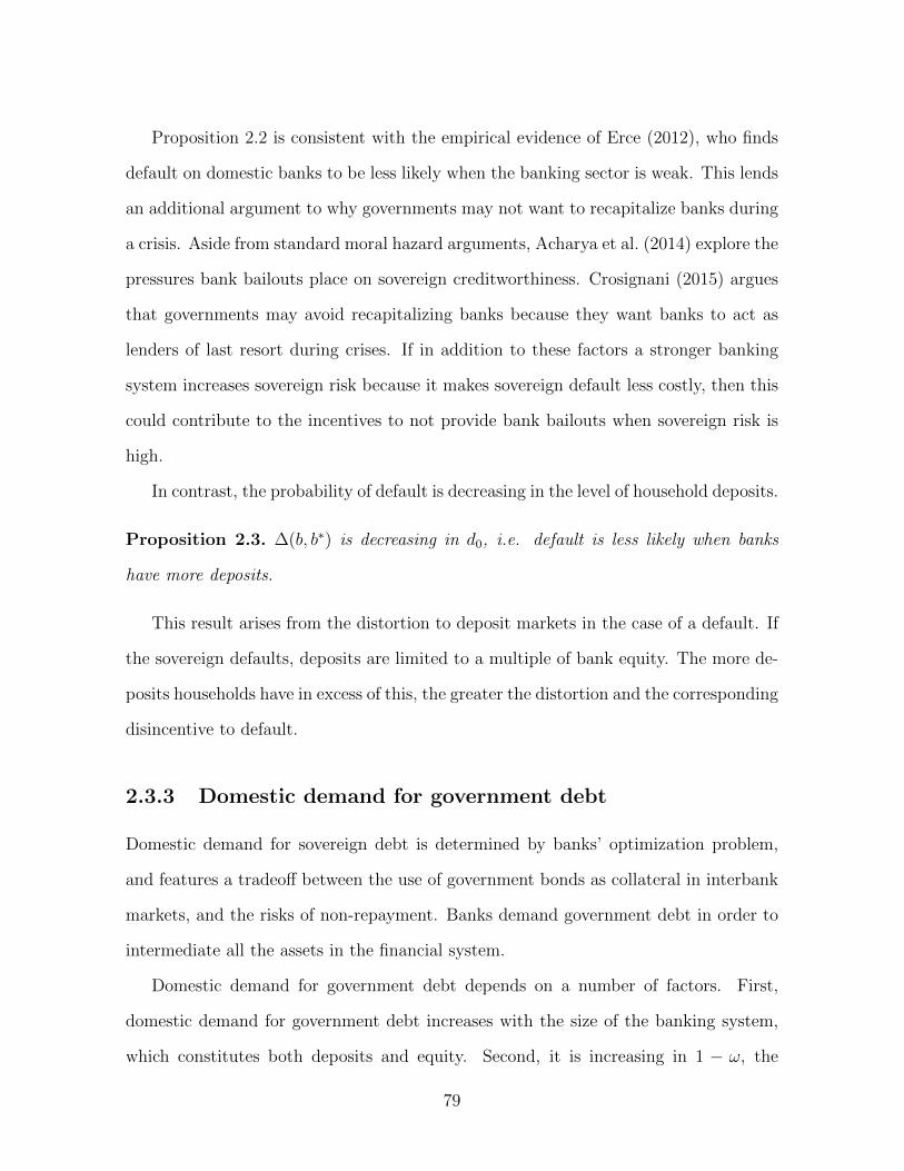
Proposition 2.2 is consistent with the empirical evidence of Erce (2012), who finds

default on domestic banks to be less likely when the banking sector is weak. This lends

an additional argument to why governments may not want to recapitalize banks during

a crisis. Aside from standard moral hazard arguments, Acharya et al. (2014) explore the

pressures bank bailouts place on sovereign creditworthiness. Crosignani (2015) argues

that governments may avoid recapitalizing banks because they want banks to act as

lenders of last resort during crises. If in addition to these factors a stronger banking

system increases sovereign risk because it makes sovereign default less costly, then this

could contribute to the incentives to not provide bank bailouts when sovereign risk is

high.

In contrast, the probability of default is decreasing in the level of household deposits.

Proposition 2.3. ∆(b, b∗) is decreasing in d0, i.e. default is less likely when banks

have more deposits.

This result arises from the distortion to deposit markets in the case of a default. If

the sovereign defaults, deposits are limited to a multiple of bank equity. The more de-

posits households have in excess of this, the greater the distortion and the corresponding

disincentive to default.

2.3.3 Domestic demand for government debt

Domestic demand for sovereign debt is determined by banks’ optimization problem,

and features a tradeoff between the use of government bonds as collateral in interbank

markets, and the risks of non-repayment. Banks demand government debt in order to

intermediate all the assets in the financial system.

Domestic demand for government debt depends on a number of factors. First,

domestic demand for government debt increases with the size of the banking system,

which constitutes both deposits and equity. Second, it is increasing in 1 − ω, the

79

extent of assets to be borrowed from nonproductive banks. Third, domestic demand for

government debt decreases in the “haircut” applied to collateral λ: the larger amount

of interbank loans that can be collateralized by one unit of sovereign debt, the lower is

domestic demand.

bopt

q

(1−ω)(n0+d0)λ

ω(n0 + d0)

Figure 2.4: Domestic demand for government debt

Fourth, if bond prices fall, more domestic debt is required to provide adequate

collateral for the banking system. Following equation 2.7, this relationship is shown in

Figure 2.4. Since the price of government bonds q is decreasing in the probability of

default p, domestic demand for sovereign debt may increase with sovereign risk.

Proposition 2.4. Domestic demand for government debt b is weakly increasing in

sovereign risk p.

This dynamic derives from the idea that increased sovereign risk lowers the value

of a “safe” asset or collateral. As the value of collateral falls, banks require more of it

in order to borrow the same amount on interbank markets. The expected return on

government debt is always R, so risk-neutral banks prefer government bonds over an

alternative safe asset that pays a return R but cannot be used as collateral.

Realistically, other safe assets can likely also be used as collateral, so that banks

can substitute away from risky sovereign debt. I discuss this bias and the possibility of

80

alternative collateralizable safe assets in Section 2.5.

In addition, this model provides a simple lens through which to consider the observed

heterogeneity in bank exposures to domestic sovereign debt. As European countries ex-

perienced increases in the risk profile of their debt, there was a concurrent repatriation

of sovereign ownership from foreign to domestic investors. Brutti and Saure (2014)

document the recent European repatriation of sovereign debt in greater detail, and ar-

gue that the evidence is consistent with secondary market theory, rather than standard

theories of portfolio allocation or home bias. Some of the increases in exposure may be

driven by banks being forced to hold additional debt, as argued by Becker and Ivashina

(2014). However, to the extent that domestic banks require sovereign bonds to collat-

eralize interbank lending, rising sovereign risk can also lead to increases in domestic

demand due to effects on the value of collateral.

Another way to characterize demand for b is to consider domestic holdings as a

share of the total face value of debt raised by the government. As shown in Figure

2.5, for low levels of total debt, domestic banks demand the full share. Once b = bopt,

this demand levels off, and there is a region over which each marginal bond issued by

the government is purchased by foreigners. This can be described as a “safe borrowing

region,” in that q = 1/R for some range of total issuance btot ∈ (∗, ∗∗) . Once b∗ reaches

a certain level, debt becomes risky, and as btot increases, p increases, which increases

domestic demand for sovereign debt b.

2.3.4 Foreign lending and bond prices

With respect to foreign debt, default is increasingly likely for higher levels of borrowing

from foreigners. This is consistent with canonical models of sovereign default.

Proposition 2.5. For b∗ < b∗′, ∆(b, b∗) ⊆ ∆(b, b∗′), i.e. the default set is increasing

in the level of borrowing from abroad.

81

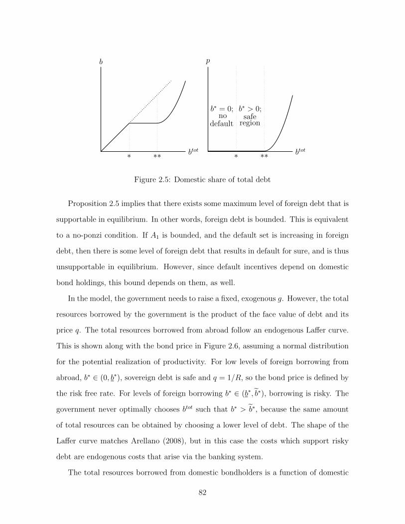
btot

b

∗ ∗∗

p

btot∗∗

b∗ = 0;no

default

∗

b∗ > 0;safe

region

Figure 2.5: Domestic share of total debt

Proposition 2.5 implies that there exists some maximum level of foreign debt that is

supportable in equilibrium. In other words, foreign debt is bounded. This is equivalent

to a no-ponzi condition. If A1 is bounded, and the default set is increasing in foreign

debt, then there is some level of foreign debt that results in default for sure, and is thus

unsupportable in equilibrium. However, since default incentives depend on domestic

bond holdings, this bound depends on them, as well.

In the model, the government needs to raise a fixed, exogenous g. However, the total

resources borrowed by the government is the product of the face value of debt and its

price q. The total resources borrowed from abroad follow an endogenous Laffer curve.

This is shown along with the bond price in Figure 2.6, assuming a normal distribution

for the potential realization of productivity. For low levels of foreign borrowing from

abroad, b∗ ∈ (0, b∗), sovereign debt is safe and q = 1/R, so the bond price is defined by

the risk free rate. For levels of foreign borrowing b∗ ∈ (b∗, b∗), borrowing is risky. The

government never optimally chooses btot such that b∗ > b∗, because the same amount

of total resources can be obtained by choosing a lower level of debt. The shape of the

Laffer curve matches Arellano (2008), but in this case the costs which support risky

debt are endogenous costs that arise via the banking system.

The total resources borrowed from domestic bondholders is a function of domestic

82

b∗

q

b∗

qb∗

b∗

1R

b∗b∗

Risky borrowing region

Figure 2.6: Bond price and total resources borrowed from abroad

banks’ characteristics. From equation (2.7) and Proposition 2.4, qb = (1−ω)(n0+d0)/λ.

As a result, the total resources borrowed from domestic banks does not change with q,

but the face value of domestic debts increases mechanically as q declines.

In the model, the exogenous level of g and the characteristics of the banking system

then pin down the optimal b, which jointly determines the specific amount of resources

that need to be borrowed from abroad and the bond price. Since the level of government

spending g must be met, whatever the government does not get willingly from domestic

banks, it must seek from abroad. An illustrative example of this is shown in Figure 2.7.

To understand the effect of domestically held debt on both the potential and realized

level of borrowing, consider an exogenous change in the characteristics of the banking

system such that more sovereign debt is naturally demanded by domestic agents. This

could be a decrease in ω or λ, or an increase in n0 or d0. In this case, the additional

domestic debt b′ > b lowers the probability of default for any given level of b∗, so q

83

b∗

q(b+ b∗)

b∗

g

b∗

Domestic share

Foreign share

Figure 2.7: Total resources borrowed

rises. The effect that this shift has on the total resources borrowed is shown in Figure

2.8. An increase in b shifts the endogenous Laffer curve up and out, leading to a larger

range of possible government spending, and shifts the risky borrowing region to the

right.

2.3.5 Default in equilibrium

Domestic debt discourages, but does not prevent default. This is a direct implication

of Lemma 2.3. Whether default may occur in equilibrium depends in particular on the

fiscal needs of the government in t = 0, and the characteristics of the banking system.

Proposition 2.6. Default can occur in equilibrium, in spite of large domestic holdings

of sovereign debt.

Whether default occurs in equilibrium depends on the realization of A1 and the

parameters of the model, and in particular the level of government spending g. If

the government were to choose g optimally, in this setting there is no incentive to

borrow from abroad, because government spending does not enter the households utility

84

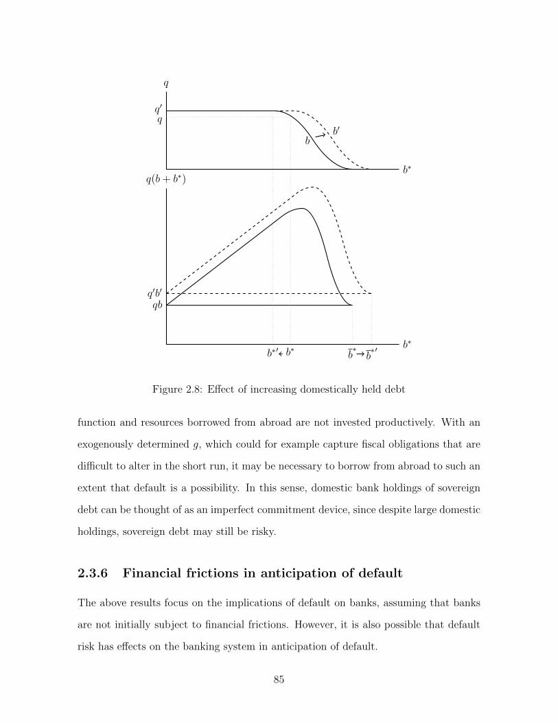
b∗

q

bb′

b∗

q(b+ b∗)

qbq′b′

b∗b∗′

q′

q

b∗b∗′

Figure 2.8: Effect of increasing domestically held debt

function and resources borrowed from abroad are not invested productively. With an

exogenously determined g, which could for example capture fiscal obligations that are

difficult to alter in the short run, it may be necessary to borrow from abroad to such an

extent that default is a possibility. In this sense, domestic bank holdings of sovereign

debt can be thought of as an imperfect commitment device, since despite large domestic

holdings, sovereign debt may still be risky.

2.3.6 Financial frictions in anticipation of default

The above results focus on the implications of default on banks, assuming that banks

are not initially subject to financial frictions. However, it is also possible that default

risk has effects on the banking system in anticipation of default.

85

If bank equity is low enough in t = 0, then households choose to limit the deposits

they channel to the banking system. This can be thought of as a form of deposit

flight. Importantly, this reduces the funds available to the banking system to invest,

which lowers potential output. This highlights an important limitation of Proposition

2.2. While weaker banks are in general more costly to default on, if low levels of bank

equity act as a constraint on deposits, undercapitalized banks can be associated with

higher default risk due to deposit flight.

Proposition 2.7. Deposit flight that occurs due to financial frictions in t = 0 makes

default more likely.

If banks are sufficiently poorly capitalized that financial frictions arise in t = 0, then

households save less in the banking system and consume more in t = 0. This negatively

affects investment and output. Since households have less wealth in t = 1, there is

less at stake to be affected by a default. This highlights one way in which sovereign

and financial crises are interconnected, as sovereign risk may lead to problems in the

financial system that reinforce the default risk of the sovereign.

An additional effect of deposit flight is to reduce the size of the banking system

(n0 + d0), which causes the level of debt demanded domestically to fall. This also

contributes to heightened default risk, in that a greater portion of fiscal needs may

need to be raised from foreign lenders. Alternately, it may increase the desirability of

financial repression, as discussed in the next section.

2.4 Externalities and financial repression

In setting domestic demand for government debt, banks do not internalize the effect

they have on default incentives. In other words, they take q as given, but q depends

on b. Taking q and A as given leads the banks’ optimization to be a problem of taking

86

expectations over intervals:

maxbE[n2] =

∫ A

A

nd2 f(A)dA+

∫ A

A

n2 f(A)dA.

In contrast, if banks were to fully internalize the effect of their debt holdings on

bond prices and the default incentives of the sovereign, then the banks’ optimization

problem would also consider the effect of their choice of b on A, p, q, and b∗. This

affects the banks’ expectations of equity in the cases of default and no default, as well

as the threshold A. In this case, solving the banks’ problem requires first integrating

and then taking a first order condition with respect to b.

In this section, the model is altered slightly to accommodate a specific form of gov-

ernment intervention in domestic sovereign debt markets, financial repression. Assume

now that the government chooses b for the banks, which changes the government’s op-

timization problem in equation (2.4) to a maximization over b and b∗, rather than over

just btot, which can be written in terms of intervals:

V0 = maxb,b∗

[c0 +

∫ A(b)

A

V d1 f(A)dA+

∫ A

A(b)

V1 f(A)dA

].

Because domestic banks do not internalize the effect of their holdings on default risk,

the government may have an incentive to choose a higher level of domestic bond holdings

than the banks choose on their own. This increases the potential cost of default, which

increases the prices at which the government issues debt. At the expense of crowding

out private investment, the government can lower its tax bill in t = 1.

When the government increases domestic holdings of sovereign debt from b to b′,

the effects can be understood in the following way. The reduction in external debt b∗ to

b∗′ comprises two effects: a mechanical reduction in b∗ which occurs because the total

fiscal need g is fixed, and an effect via improvement in the price:

db∗

db= −

[1 +

g

q2

dq

db

]< 0.

87

From Proposition 2.1, an increase in domestic bond holdings decreases default risk,

dq/db > 0, and thus db∗/db < 0.

However, any increase in b beyond the amount required to intermediate all the assets

in the banking system leads to crowding out:

dk1

db= −

[dq

dbb+ q

]< 0.

Since q ∈ [0, 1R

] and dq/db > 0, this is unambiguously negative, as well. Whether finan-

cial repression has the potential to improve welfare depends on whether the reduction

in external debt outweighs the cost of crowding out.

Proposition 2.8. When debt is risky, financial repression crowds out private invest-

ment, but can improve welfare. A necessary condition under which financial repression

can improve welfare is:

dV1

db

∣∣∣∣b= (1−ω)(n0+d0)λq

> 0 .

The idea behind Proposition 2.8 is shown in Figure 2.9, for an increase in domestic

bond holdings from b to b′. It is possible that despite crowding out private investment,

the decrease in the face value of foreign debt that this achieves will increase welfare if the

realization of productivity is such that default does not occur. Financial repression also

lowers the threshold A below which default occurs, which leads to welfare improvements

for productivity realizations between A′ and A.

However, for realizations of productivity below the new threshold, financial repres-

sion leads to an unambiguous decrease in welfare. This perhaps relates to historical

default episodes such as Argentina in 2001 or Russia in 1998. In these latter two default

episodes, domestic banks seem to have piled up on domestic debt, only to then suffer

even greater losses when the respective defaults took place (Basu, 2010). In some sense,

88

AAA′

V1

V ′1

V d1

V d1′

Figure 2.9: Financial repression can increase welfare

financial repression can be seen as taking a gamble that does not necessarily prevent

default, and which makes outcomes all the more worse if default occurs.

In addition, the improvements in welfare that result from financial repression are

decreasing in the realization of A1. This can be shown by the negative second derivative:

d2V1

dbdA1

= A2

[−dqdb− q]< 0.

Although there may then be some range of productivity realizations over which finan-

cial repression improves welfare, for high realizations of productivity the losses due to

crowding out increase relative to the gains of reduced external debts.

Finally, there are also realizations of A1 in which despite avoiding default, welfare

declines. This is shown in area of Figure 2.9 where A1 is higher than A′, where V ′1 is

lower than V d1 . Overall, there are limits to the extent to which financial repression can

be relied upon to avoid a potential default.

This section relates to the findings of Chari et al. (2015), who argue that when the

government cannot commit to repay debts, financial repression may be optimal. In

their model, regulation motivates bank holdings of government bonds. While the basic

intuition of domestic bank holdings of sovereign debt as commitment is the same, in

this setting banks have an added motive to hold government debt as collateral. As

89

such, financial repression must be understood as inducing demand above and beyond

what banks would choose to invest in on their own.

With risk-averse households and centralized borrowing (where the government trans-

fers its borrowings to households, instead of spending it on g directly), financial repres-

sion can have further benefits in terms of facilitating the ability of households to smooth

consumption. In this case, by increasing domestically held sovereign debt, the govern-

ment can borrow more from abroad, benefiting its citizens directly. A related case is

explored in Section 2.5, where foreign lenders can channel capital inflows to banks.

2.5 Extensions

Two limitations of the model are that domestic sovereign debt is assumed to be the

only eligible type of collateral, and that foreign capital is borrowed exclusively by the

government, while in reality banks and firms also receive foreign inflows. In this section,

I first discuss the implications of allowing a second safe asset to be used as collateral, and

then argue that allowing banks to borrow from abroad in addition to the government

reinforces the main mechanisms described in Sections 2.3 and 2.4.

2.5.1 Second safe asset

An easy objection to the role of sovereign debt as collateral in motivating demand for

domestic sovereign debt is the presence of alternative safe assets, for example, U.S.

Treasuries. If banks are able to costlessly use alternative safe assets as collateral in

interbank transactions, then there is little motive to invest in risky domestic sovereign

debt. When other assets can also be used as collateral, they could in theory confer all

of the same benefits as domestic sovereign debt, and have none of the associated risks.

Under the assumption that a second safe asset is available and completely safe,

and if domestic sovereign debt is risky, domestic banks in this model would strictly

90

prefer to use the safe asset instead of the domestic one. In this situation, some form of

regulation, moral suasion, or financial repression would be necessary to have non-zero

domestic holdings of sovereign debt. As discussed in Section 2.4, there is some scope

to undertake these policies while improving overall welfare. Where second safe assets

are perfect substitutes for domestic sovereign debt, financial repression is necessary to

enable the government to raise its fiscal needs g. However, in the presence of regulations

that require domestic intermediaries to hold domestic sovereign debt, or that provide

incentives for domestic government bondholdings over foreign alternatives, banks face

a tradeoff between these factors and the risks of non-repayment.

It may also be that banks can more easily invest in domestic sovereign debt due to

issues of proximity, exchange risk, jurisdiction, etc. Diversification of sovereign debt

within a bank’s portfolio may require infrastructure in which the bank must invest,

raising the barriers to doing so. This would lessen the need for explicit financial repres-

sion.

More generally, it is worthwhile to consider to what extent alternative safe assets

exist. Some have noted the apparent shortage of safe assets in the global economy

(Caballero et al., 2008; Caballero and Farhi, 2015), as well as the consequences of low

public debt issuance for the creation of private “safe” securities (Krishnamurthy and

Vissing-Jorgensen, 2012, 2013). Issues such as these complicate the ability of banks to

diversify sovereign debt holdings. To the extent that banks and investors demand “safe”

assets that are in limited global supply, a security with government backing may be

an acceptable alternative. Such preferences are also consistent with “risk-shifting” by

banks that maximize their profits, conditional on the absence of a government default.

91

2.5.2 Capital inflows to banks

In many countries, a substantial portion of capital inflows are intermediated by banks

rather than flowing directly to the government. Allowing banks to borrow from abroad

generates some additional implications in the framework of this model.

Assume that foreign lenders are now willing to lend to domestic banks in whole-

sale markets, and that these loans go into specific foreign-owned investment projects.

Consider foreign lending to be similar to domestic interbank lending, in that it requires

collateral in the form of government debt and occurs at some (foreign) haircut. At

the outset, providing an additional role for collateral would likely increase the domes-

tic demand for sovereign assets, depending of course on the presence of alternative

collateralizable securities.

If foreign inflows to banks pay a return that is fixed in advance, a low realization of

productivity can lead to even lower equity in the banking sector. This would lead either

to financial frictions that are more severe, or in some cases, solvency problems for the

banking sector, which may then default on its obligations. One could consider whether

bank defaults lead the government to step in and guarantee private sector debts, as

occurred in Ireland. If so, a private sector default could precipitate a sovereign default,

linking financial and sovereign crises.

Suppose that a sovereign default leads the private sector to also default. This is

often effectively the case following a sovereign default due to policies implemented to

prevent capital from flowing out of the country, such as deposit freezes, capital controls,

and/or exchange controls. In this case, sovereign risk is tied to private risk, and so

when sovereign risk rises it has the additional negative effect of limiting inflows into the

banking system. This provides an additional benefit for policies that reduce sovereign

risk, such as financial repression, because they facilitate the intermediation of private

capital flows to productive investment.

92

A related policy introduced in the recent European crisis was the provision of long-

term refinancing operations (LTROs). Specifically, these refinancing operations offered

euros to banks in exchange for a wide array of collateral, including peripheral govern-

ment debt. This was aimed to prevent liquidity shortages at European banks, but is

shown by Crosignani et al. (2015) to have contributed to increased bank sovereign expo-

sures. By providing an additional role for collateral, LTROs increased banks’ holdings

of domestic sovereign debt.

The banking sector is critical to both facilitating productive investment and also

mitigating sovereign risk, and when banks also borrow from abroad, there is more at

stake in a sovereign default. LTROs can be thought of as providing not only liquidity,

but also as an additional driver of domestic exposure to sovereign debt, and thus reduced

default risk. However, this may also worsen outcomes in the event of default, since

domestic banks are more exposed to sovereign risk.

2.6 Conclusion

In this chapter, I present a model of domestic banks and sovereign default that illus-

trates the role of domestic banks in supporting risky sovereign debt, through endogenous

output losses that result from sovereign default. This provides a specific microfoun-

dation for a political economy argument made in secondary market theory, and a new

lens through which to consider the recent trends in ownership of government debt in

the European periphery. In addition, the model predicts that default incentives are

tied to the health of the banking system and the level of borrowing from abroad, and

demonstrates that there are cases where policies such as financial repression can be

welfare improving. Importantly, while domestic holdings of sovereign debt can be un-

derstood as strengthening commitment, sovereign governments may default in spite of

large domestic exposures to their debt.

93

In a number of ways, this model is highly stylized and should be taken with a

full understanding of its limitations. The treatment of the substitutability of domestic

and foreign safe assets is simplistic, default is assumed to be non-selective, and bank

recapitalizations are ruled out. I assume banks do not default as a result of a sovereign

default. In a sense, the results may then be a lower bound on the endogenous cost

of sovereign default, assuming that outright bank failures are more disruptive than

financial frictions.

It would be useful to further explore the quantitative importance of the mechanisms

described in this chapter. For example, it would be interesting to test how much of

a quantitative effect incremental increases in domestic bond holdings have on default

incentives, conditional on the existing level of exposures. It would also be informative

to compare how the costs of financial frictions compare to disruptions to interbank

lending, or to multi-period exclusion from international financial markets. I leave these

questions to future work.

94

Chapter 3

Matching in corporate loan markets

and macroeconomic shocks

95

3.1 Introduction

What is the effect of bank-firm matching on economic outcomes, such as lending, lever-

age, and output? In this paper, I develop an assignment model of the corporate lend-

ing market, with heterogeneous banks and heterogeneous firms. The model is used to

demonstrate an analytically tractable characterization of bank-firm matching, and to

explore the implications of macroeconomic shocks to borrowers and lenders for firm-

level, bank-level, and aggregate outcomes.

Matching in corporate loan markets is important because it has distributional im-

plications for the transmission of shocks, and because matching can lead to bias in

empirical work using loan-level data. For example, if certain banks are relatively more

affected by monetary policy shocks, this could disproportionately affect a particular

subset of firms. In empirical work, inference about the effects of bank shocks depends

on assumptions about matching, because of the potential for confounding treatment

and selection effects. An ability to better characterize matching patterns in corporate

lending would be helpful both in understanding distributional consequences of shocks

and improving empirical estimates of their effects.

To demonstrate a tractable theory of matching between banks and firms, I develop

a model that builds on Holmstrom and Tirole (1997), with the additional assumptions

of (i) heterogeneity among financial intermediaries and (ii) firms with heterogeneous

productivity levels. There are two periods, and three types of agents: a continuum of

firms, a continuum of banks, and uninformed investors. In the first period, firms seek

loans in order to undertake investment projects. Firm investments depend on both firm

and bank characteristics, and include internal firm capital, loans from intermediaries,

and loans from uninformed investors. In the second period, returns are realized and

claims are settled. All parties are risk neutral and assumed to be protected by limited

liability.

96

Banks start with some initial capital, i.e. equity, and higher skill banks monitor at

a lower cost. Uninformed investors are only willing to lend alongside banks, and can be

thought of as depositors or other funding sources for the banking system. With some

probability, successful projects generate a return that is constant returns to scale but

depends on firm productivity. Otherwise projects return zero. There is assumed to be

a double moral hazard problem, in that the probability of a project’s success is higher

if firm managers exert effort and the bank monitors, and both actions come at a cost.

Matching in the model is determined as follows: firms choose a bank and its asso-

ciated lending terms to maximize profits, and banks set loan terms and select firms in

order to maximize returns. The moral hazard problems pin down the returns paid to

firm managers and banks, and thus the investment size chosen by each firm. Investment

size increases in both firm productivity and bank skill. Higher productivity firms are

able to pledge more future profits to attract uninformed investors. Similarly, higher

skill banks require less absolute return to maintain incentive compatibility, leaving a

greater share of future profits to be pledged to uninformed investors.

In particular, firms’ investments are log-supermodular in firm productivity and bank

skill. This facilitates drawing from methods that have been adopted in matching theory

and models in international trade, which explore comparative statics predictions that

result from log-supermodularity (e.g. Costinot, 2009; Costinot and Vogel, 2010). One

contribution of this chapter is to show that the same mathematical property also has

useful applications for modeling financial intermediaries.

In equilibrium, there exists a continuous and strictly increasing matching function

that maps firms to banks. The matching function is defined in terms of an ordinary

differential equation determined by market clearing. Although the matching result is

strict in that it matches each firm to one bank, and predicts perfect sorting, this can

be relaxed in a number of ways. If banks limit the size of their exposure to any one

97

particular firm, firms are matched with an interval of banks, whose endpoints are weakly

decreasing in firm productivity. Alternately, if banks are subject to idiosyncratic shocks

that occur after matches have been determined, but before lending disbursements, firms

have an incentive to diversify their borrowing partners. Finally, if the characteristics of

banks or firms are not perfectly observable, less strict patterns of matching are obtained.

For simplicity, I focus on the basic prediction of strict matching, but expect that the

model predictions follow for richer cases, as well.

Based on the matching that occurs in competitive equilibrium, I demonstrate a

number of reasons why matching and its impact on lending is important. First, the

model predicts positive assortative matching in firm productivity and bank skill. High

skill banks have a tendency to lend to high quality firms, so low skill banks are only

able to capture a low quality segment of the market. As a result, it is likely that bank

portfolios are concentrated, in the sense that firms of a particular type tend to borrow

from the same or similar banks.

Second, better banks are also more able to leverage their own capital, and thus

can lend to a wider range of projects. This implies that the capital available to high

productivity firms is greater than that of other firms, which cannot take advantage of

higher skilled bank capital because of capacity constraints on high productivity banks.

This leads not only to higher leverage among high bank and firm types, but amplifies

the advantages that high types have, since they also benefit from assortative matching.

Third, the model facilitates a number of interesting comparative statics predictions.

A positive productivity shock to firms leads to a decrease in lending to existing firms,

and a decrease in lending on the extensive margin. This is because higher productivity

firms crowd other firms out of borrowing from top banks. The model shows how

capital inflows can lead to different effects, depending on whether inflows are managed

by uninformed investors or banks. In particular, if capital flows principally to banks,

98

this leads to increases in both intensive and extensive margin lending, and thus declines

in overall credit quality. Finally, a reallocation of capital from high to low skill banks

leads to a decrease in both intensive and extensive margin lending, and increases in bank

leverage that are more pronounced among banks of lower skill. This has implications

for financial regulation, and how regulations that focus on large banks may affect all

firms in the economy, and lead to leverage increases at smaller banks.

The rest of the chapter is structured as follows. In the remainder of this section

I review the relevant related literature. Section 3.2 presents the model. Section 3.3

discusses the applications. The final section concludes.

3.1.1 Related literature

This chapter relates to two broad categories of research, the first being financial inter-

mediation. How credit disruptions impact the broader economy has been a subject of

economic interest since at least the Great Depression.1 It has been shown how bank

shocks can have real effects in theoretical and empirical settings. Of the many existing

models of financial intermediation, in this chapter I take as a basis Holmstrom and

Tirole (1997).

At the same time, many researchers have shown that banks gain firm-specific in-

formation via lending, which leads to “stickiness” in bank-borrower relationships. This

leads to less than perfect substitutability between loans from different banks, since cost

and effort are required to establish new relationships with lenders.

While much of the aforementioned research recognizes that banks and firms are

in some sense searching for and matching with lending partners, there are only a few

papers that study two-sided matching between banks and firms explicitly. Chen and

Song (2013) provide empirical evidence that geographic proximity, sizes, and prior loan

1For example, see Fisher (1933).

99

relationships are important drivers of lending partners. Chen (2013) explores the conse-

quences of matching for loan spreads. Duprey (2016) models two-sided group matching

between banks and entrepreneurs, but focuses on screening efficiency and explores im-

plications for aggregate productivity and lending fluctuations. I model matching in a

static context, and focus mainly on implications for matching, leverage, and output.

Financial frictions have also been incorporated into models to demonstrate how

intermediaries can amplify business cycles and in particular worsen economic slumps.

The canonical models in this class are Bernanke et al. (1999) and Kiyotaki and Moore

(1997). Ultimately, allowing for cross-sectional variation in the quality of banks’ en-

dogenous portfolios may be valuable in considering changes in aggregate credit quality,

and how these changes contribute to cyclicality. I see this chapter as a first step in this

direction, although I abstract from dynamics in this setting to show implications in a

static context.

The second research area to which this chapter relates is search and matching.

Search and matching models are increasingly applied in labor markets (Menzio and

Shi, 2011; Kaas and Kircher, 2015) and international trade (e.g. Davis and Dingel,

2012). There are also applications of these methods to specific financial markets, e.g.

OTC markets (Duffie et al., 2005). Ottonello (2017) models search in markets for

physical capital, which he shows can contribute to the persistence of recessions. This

chapter relates most closely to this work, but takes as its object bank loans, or financial

capital, which firms require to invest. In particular, I draw from methods which have

been adopted in models in international trade, which explore comparative statics that

result from the assumed property of log-supermodularity (Costinot, 2009; Costinot and

Vogel, 2010). The contribution of this chapter is to show that the same mathematical

property also has useful applications for modeling financial intermediaries.

100

3.2 Model

The model has three types of agents: firms, intermediaries, and uninformed investors.

This section builds on Holmstrom and Tirole (1997) by adding (i) heterogeneity among

financial intermediaries and (ii) firms with heterogeneous productivity levels, in order

to explore the pattern of matching and its consequences.

There are two periods. In the first period, financial contracts are signed and invest-

ment decisions are made. In the second, returns are realized and claims are settled. All

parties are risk neutral and protected by limited liability.

3.2.1 Firms

Firms are endowed with one unit of initial capital and vary in terms of the rate of return

r ∈ R that they generate if their projects are successful. The distribution of potential

firms with return r is denoted F(r) ≥ 0. Of these, a subset F ⊂ F obtain financing,

and there is some productivity cutoff below which firms are unable to obtain external

funds. The firms that obtain external financing are denoted by R ≡ {r ∈ R|F (r) > 0}.

Firms borrow from banks and uninformed investors to make an investment of vari-

able size I(s, r), where s indexes the skill of the bank, and r indexes the return on

investment of each firm. The funds to be invested include one unit of internal firm

capital, plus investments from intermediaries Im and uninformed investors Iu:

I(s, r) = 1 + Im + Iu. (3.1)

Successful projects generate a return of rI. Otherwise projects return zero. The

probability of success when firm managers exert effort is denoted by pH , and if they do

not, pL < pH . It is assumed that ∆p = pH − pL > 0. In the absence of incentives, firm

managers may choose to exert less effort. Formally, entrepreneurs choose between two

versions of the project, shown in Table 3.1.

101

Table 3.1: Available projects

Project Good BadEffort required per unit of investment e 0Probability of success pH pL

The returns on investment are used to make payments to each group:

rI(s, r) = Rf +Rm +Ru. (3.2)

For it to be incentive compatible for firm managers to exert effort, firms’ internal

return must satisfy:

Rf (r) ≥eI(s, r)

∆p. (ICf )

The problem of an individual firm is to choose Im, Iu, Rm and Ru to maximize:

πf (r) = rI(s, r)−Rm −Ru − eI(s, r). (3.3)

When combined with equation (3.2), equation (3.3) is equivalent to maximizing Rf ,

which is bounded below by (ICf ). Since managers must be compensated for the effort

they exert, and their effort is increasing in the size of the investment, individual firm

managers have an incentive to maximize the size of their investment project. This is

equivalent to maximizing the leverage obtained from banks and uninformed investors

in equation (3.1).

3.2.2 Banks

Banks exist on a continuum indexed by skill s ∈ R. Banks of skill s have capital

km(s) available to lend, and choose borrowers in order to maximize expected profits. In

particular, a bank with higher skill monitors projects more efficiently: it costs a better

bank less to monitor projects. This cost is denoted by c(s), which is decreasing in skill

c′(s) < 0. The equilibrium rate of return on bank loans is denoted by β.

102

Banks are also assumed to be subject to moral hazard. For it to be incentive

compatible for the bank to monitor, it must be that they are paid a return Rm(s):

Rm(s) ≥ c(s)I(s, r)

∆p, (ICm)

where c(s) is the monitoring cost for a bank of skill s. The incentive constraint (ICm)

implies that banks earn positive profits. As in Holmstrom and Tirole (1997), I assume

that competition reduces this surplus by forcing monitors to contribute to the firms’

investment in the first period. The expected return on intermediary capital must be at

least the market return β:

pHRm ≥ βIm, (3.4)

where β is set in equilibrium so that the market for informed capital clears. Combining

(ICm) and (3.4) gives the bank loan as a function of bank skill s, firm productivity r

and success probability pH and ∆p, and the market return β:

Im(s, r, β) =pHc(s)I(s, r)

β∆p. (3.5)

The problem of a bank is to choose which firms to lend to, and how much to lend.

For each bank s ∈ S, the bank’s problem is to choose borrowers and loan sizes to

maximize profits:

Πm(s) =

∫r∈R

[pHRm(s, r)− c(s)I(s, r)]L(s, r)dr, (3.6)

subject to a budget constraint:

km(s) =

∫r∈R

Im(s, r)L(s, r)dr, (3.7)

where L(s, r) is the number of firms with return r to which banks with skills s lend.

The bank choice of borrowers sets the function L(s, r).

103

At minimum, β must be high enough that banks prefer monitoring to investing

capital in the open market, where it would earn a return of γ:

γIm = γ

[pH c(s)I(s, r)

∆pβ

]≤ pH c(s)I(s, r)

∆p− c(s)I(s, r).

This sets the minimum β:

β = pHγ/pL. (3.8)

If the banking sector is perfectly competitive, i.e. with free entry at each level of

skill, banks at each skill level will earn this minimum return β. 2

3.2.3 Uninformed investors

Uninformed investors in the economy are willing to invest alongside a bank, but unable

to monitor. As such, they earn a lower rate of return γ < β, where γ is set exogenously

by some other instrument in which uninformed investors can invest, such as a risk

free bond.3 Uninformed capital can be thought of as banking sector liabilities, such as

deposits, wholesale funding, or interbank loans.

The maximum income that can be pledged to uninformed investors while maintain-

ing incentive compatibility must be enough to pay uninformed investors a return γ on

their contribution to the project:

pHRu ≥ γIu. (ICu)

2The main results of the chapter also hold if the return β varies in skill. This would correspondto cases in which there is imperfect competition, so long as banks do not act as monopolists. In themonopolistic case, banks can extract all the surplus that firms gain from borrowing from a betterbank, as a result of which investment sizes are no longer increasing in bank skill. The case with β(s)is shown in the Appendix.

3Alternately, γ can be set in equilibrium when faced with a supply schedule for uninformed capital.

104

Suppose (ICf ) and (ICm) bind. The maximum return which can be promised to

uninformed investors is therefore:

Ru(s, r) = I(s, r)

[r − e+ c(s)

∆p

]. (3.9)

Since uninformed investors are assumed to have an opportunity cost of γ, this pins

down the maximum investment possible from uninformed investors:

Iu(s, r, γ) =pHRu(s, r)

γ. (3.10)

Combining equations (3.9) and (3.10) it is evident that the maximum share of funds

available from uninformed investors is increasing in both bank skill and firm produc-

tivity, as shown in Figure 3.1.

r

IuI

s

IuI

Figure 3.1: Share of uninformed capital

Higher productivity firms have more returns available to pledge to uninformed in-

vestors, and are therefore are able to attain a greater share of leverage from them.

Higher skill banks have a lower per unit cost of monitoring, and so require lower re-

turns to maintain incentive compatibility. As a result, more returns can be pledged to

attract uninformed investors if a firm is matched with a high skill bank. These patterns

will subsequently drive the overall investment size of firms to be increasing in r and s,

as shown in the following section.

105

3.2.4 Competitive equilibrium

With these assumptions about banks and uninformed investors, the maximum level of

investment that a firm can make is given by combining (3.1), (3.5), (3.9), and (3.10) to

obtain:

I(s, r) =1

1− pH c(s)β∆p

− pHγ

[r − e+c(s)

∆p

] . (3.11)

The investment of a firm is also a measure of firm leverage, since each firm is endowed

with one unit of capital. For example, if both types of capital are infinitely expensive,

i.e. β = γ = ∞ the firm cannot borrow at all. As the denominator above approaches

zero, the size of the total investment goes to infinity. The two fractions that enter

negatively in the denominator of equation (3.11) reflect the share of I(s, r) contributed

from informed and uninformed investors, respectively.

Since γ < β, firm managers prefer to maximize the investment from uninformed

capital rather than bank loans. As a result, (ICm) will bind, i.e. banks will be paid the

minimum that is incentive compatible for them to monitor. To maximize firm profits,

it is also optimal that (ICf ) binds, because firm returns are also increasing in total

investment size. Paying more than the minimum (ICf ) reduces the returns available to

be pledged to uninformed investors, and therefore the total investment size. As a result,

the firm problem can be stated as maximizing (3.3) subject to (3.1), (3.2), (3.4), (ICf )

and (ICm) holding with equality, (3.9), and (3.10). Equivalently, (3.11) can be taken

as the maximal level of investment that result from the firm optimization problem.

From equation (ICm), banks’ returns are increasing in the size of the firm’s in-

vestment. This gives banks an incentive to lend to projects that are of the highest

productivity possible given the firms and other banks in the economy.4 From equations

(3.4) and (3.11) it is possible to see a basic form of complementarity: the size of an

4When β is uniform this preference is weak; it is a strict preference when β is a function of skill.

106

investment depends positively on both bank skill s and firm productivity r.

Lemma 3.1. Investment size is increasing in both s and r, i.e. dI/ds > 0 and dI/dr >

0.

Proof. All proofs are included in the Appendix.

As bank skill increases, the cost of monitoring declines, which leaves firms with

more returns that can be pledged to uninformed investors. A high skill bank makes

a smaller loan because it has a lower monitoring cost, and so requires a lower gross

return to maintain incentive compatibility. Consequently, a high skill bank is more

able to attract leverage uninformed capital. The change in financing mix lowers the

overall cost of capital for the firm. In this way, a more efficient bank allows a firm to

undertake a larger investment. Similarly, a higher productivity firm can make a larger

investment because more funds are generated that can be used to attract investors.

These properties are shown graphically in Figure 3.2.

r

I

s

I

Figure 3.2: Investment size

The complementarity between firms and banks also has a particular property that

is useful for analyzing matching between banks and firms, namely that it is log-

supermodular.

Lemma 3.2. I(s, r) is strictly log-supermodular.

107

Log-supermodularity gives that:

I(s′, r′)I(s, r) > I(s, r′)I(s′, r) for all s′ > s and r′ > r. (LSM)

Since I is strictly positive, (LSM) can be rearranged as:

I(s′, r′)

I(s, r′)>I(s′, r)

I(s, r).

Lemma 3.2 states that high productivity firms benefit relatively more from matching

with a high skill bank. In other words, high-skill banks have a comparative advantage in

lending to high productivity firms. Although the assumptions in this setup are based on

a stylized case of heterogeneity among banks and firms, this demonstrates an instance

in which the size of financed projects is complementary. Log-supermodularity is useful

because it allows for comparative static predictions to be made for broad classes of

functions which satisfy this property. Importantly, in this setting, log-supermodularity

is derived rather than assumed. To justify the application of this property in a novel

setting, I demonstrate its microfoundations in a model of firms and banks. Although

log-supermodularity is shown here using a specific model, I expect the general results

to extend to other production functions in which log-supermodularity holds.

Intuitively, log-supermodularity in this setting can be understood in a similar way

as Lemma 3.1. The relative advantage of high productivity firms in borrowing from

high skill banks derives from their ability to attract more uninformed capital compared

to low skill banks, and because this uninformed capital is relatively cheaper. Not only

do the overall loaned funds increase, but also the overall cost of capital falls.

In a competitive equilibrium, all firms and banks maximize profits, and all markets

clear. Profit maximization by firms requires:

rI(s, r)−Rm(s)−Ru(s, r)−Rf (r) ≤ 0 for all s ∈ S, (3.12)

rI(s, r)−Rm(s)−Ru(s, r)−Rf (r) = 0 for all s ∈ S s.t. L(s, r) > 0.

108

Goods market clearing:

F (r) =

∫s∈S

L(s, r)ds for all r ∈ R (3.13)

Banks:

maxL(s,r)

Πm(s) =

∫r∈R

[pHRm(s, r)− c(s)I(s, r)]L(s, r)dr for all s ∈ S. (3.14)

Lending market clearing:

km(s) =

∫r∈R

Im(s, r)L(s, r)dr for all s ∈ S. (3.15)

Formally, a competitive equilibrium is defined as follows:

Definition 3.1. A competitive equilibrium is a set of functions L : S × R → R+,

Rm : S → R+, Rf : R → R+, Im : S × R → R+, Iu : S × R → R+ and prices γ and β

such that conditions (3.12)-(3.15) hold.

3.2.5 Bank-firm matching function

The setup of the model imposes restrictions on competitive equilibria, such that it is

possible to solve for a function that matches firms and banks.

Lemma 3.3. In a competitive equilibrium, there exists a continuous and strictly in-

creasing matching function M : R→ S such that (i) L(s, r) > 0 if and only if M(r) = s,

and (ii) M(r) = s and M(r) = s.

Lemma 3.3 can be interpreted in the following way: since firm output and profits are

increasing in bank quality, firms prefer to be matched with the best bank possible. This

is because good banks have a comparative advantage in providing financing to the higher

productivity firms in the economy, and allow firms to undertake larger investments. For

example, this property could capture the fact that high productivity firms have broad

banking needs (e.g. various credit lines and loan facilities, trade credits, exchange rate

109

services, etc.) which allow it to benefit relatively more from a higher skill bank than a

low productivity firm that requires only a loan.

Importantly, the upper bounds of bank skill and firm productivity and the lower

bound of bank skill are assumed to be exogenous, but the lower bound of firm produc-

tivity is set endogenously.

The remainder of the analysis relies on the following Lemma.

Lemma 3.4. In a competitive equilibrium, the matching function satisfies

dM

dr=Im(M(r), r)F (r)

km(M(r)), (3.16)

with M(r) = s and M(r) = s.

The matching function in Lemma 3.4 is an ordinary differential equation, determined

by market clearing. The intuition for the matching function is that its slope equates

firms’ demand for capital with supply.

Importantly, the matching process in this economy leads to bank portfolios that are

concentrated and heterogeneous. Concentration derives from the fact that firms aim

to match with the best banks possible. Thus, the best banks lend to the best firms,

and for some interval of firms that are closely related in terms of productivity, they

are likely to be matched banks of similar skill. I explore this idea using two graphical

examples, shown in Figures 3.3 and 3.4.

Figure 3.3 demonstrates a simple case in which there are three banks ordered in

terms of skill, s1 < s2 < s3. Strictly speaking, discrete banks differ from the continuum

under which the results of the chapter are proved, but the basic intuition is the same.

For simplicity, each bank has the same initial capital km(s) = km and firms are uniformly

distributed along a continuum, F (r) ∼ U [r, r]. Since Im is smaller for the bank of high

skill, the best bank can make smaller investments in a larger number of projects, leading

the banks’ range of matches in r to be increasing in skill.

110

r

s1 s2 s3

r

Figure 3.3: Matching pattern for discrete banks

r

F(r)

Firm distribution

ss

km(s)

Capital distribution

r′

s

rs

M(r)

Matching function

Figure 3.4: Firm distribution, capital distribution, and matching

A more general case is shown in Figure 3.4. For a given distribution of firms (left

panel) and capital across banks (center panel), it is possible to solve for a matching

function that takes the shape shown in the right panel. The matching function maps

firms of a particular productivity r to a bank of skill s. The concave shape stems from

the fact that Im is decreasing in skill, so in general higher skill banks are able to capture

a relatively large share of the lending market. The exact shape of the matching function

depends on not only the distribution of firms and bank capital, but also on the shape

of the cost function c(s).

Figure 3.5 shows the patterns of firm and bank leverage in equilibrium. Since firms

all begin with one unit of capital, their investment I(s, r) is also a measure of leverage.

For banks, as a proxy for leverage I use the ratio of the sum of their capital and

uninformed capital in the firm-specific investment they are mapped to, to the size of

each bank’s loan. Positive assortative matching in the economy leads to higher leverage

among the top quality banks and highest productivity firms.

The pattern of matching is strict in the sense that each firm is matched to a single

bank. This can be relaxed in a number of ways. First, banks could limit the size of

111

r′

s

rs

I(s, r)

Firm leverage

ss

Im+IuIm

Bank leverage

Figure 3.5: Firm and bank leverage

their exposure to any one particular firm, which would lead to firms being matched with

an interval of banks, whose endpoints are weakly decreasing in firm productivity. This

pattern is shown in Figure 3.6. Second, banks could be subject to idiosyncratic shocks

that occur after matches have been determined, but before lending disbursements. This

would lead to the same general pattern as in the first case. Third, if the characteristics

of banks or firms are not perfectly observable, this could lead to less strict patterns

of matching, as well. However, for simplicity I focus on the basic prediction of strict

matching, with the assumption that this general pattern follows for richer cases, as

well.

r′

s

rs

M(r)

Matching function

Figure 3.6: Multiple bank matches

112

3.3 Applications

Given the matching function characterized in Section 3.2, I now explore how a variety

of macroeconomic shocks affect the pattern of matching, lending, leverage, and output.

3.3.1 Productivity shocks

Consider a productivity shock that leads there to be more high productivity firms in

an economy, as shown in the top left panel of Figure 3.7. If banks’ capital is unaffected,

then the funds banks have available must then be allocated among a shifted distribution

of firms. This leads to a downwards shift in the matching function:

Proposition 3.1. Suppose F ′(r′)F (r) > F (r′)F ′(r) for all r′ > r. Then M ′(r) ≤M(r)

for all r ∈ R ∩R′.

The productivity shock described Proposition 3.1 causes the distribution of firms

over r to shift to the right. In response to an increase in the number of high productivity

firms, banks lend more to higher productivity firms, but this ties up bank capital in a

way that causes a downwards shift in the matching function M(r). Graphically, this

is shown in the top right panel of Figure 3.7. As a result, firms match with worse

banks. This leads to a decrease in lending on the extensive margin, in that some low

productivity firms will now be crowded out of the market.

For a given productivity level, firm leverage is lower, because firms are matched

with worse banks. Yet, bank leverage rises because banks are matched with better

firms, with larger effects on worse banks. These results are shown in the bottom panels

of Figure 3.7. Because the shift in the matching function causes firms to match with

lower skilled banks, output rises by less than the increase in productivity could generate

if banks were able to obtain additional capital. In this way, growth without financial

development may pose limits to the firms that exist in the economy.

113

To summarize, a positive productivity shock to firms in the economy causes:

1. An downwards shift in the matching function, such that firms match with worse

banks, and a decrease in lending on the extensive margin;

2. A decrease in firm leverage at a given r, with larger effects for worse firms;

3. An increase in bank leverage, with larger effects for worse banks; and

4. A less than proportional increase in overall output.

3.3.2 Uninformed capital inflows

A second application of the model is to capital inflows and credit quality. Capital

inflows and credit booms often precede financial crises (Schularick and Taylor, 2012;

Jorda et al., 2013), and also seem to lead to higher bank risk taking (Shin, 2009;

Dell’Ariccia and Marquez, 2006). This is consistent with the idea that banks’ moral

hazard problems are worsened by higher liquidity (Diamond and Rajan, 2001). This

model tells a complementary story. If the universe of potential firms is unlimited, but

r

F(r)

F ′(r)

Firm distribution

r′r′

s

rs

M ′(r)

M(r)

Matching function

r′

I ′(s, r)

rr′

I(s, r)

Firm leverages

ss

I′m+I′uI′m

Im+IuIm

Bank leverage

Figure 3.7: Productivity shock

114

high quality firms are in limited supply, then capital inflows can cause both increases

in leverage and increased lending on the extensive margin, to new lower productivity

firms.

There are two ways to consider capital inflows in the context of this model, the first

of which is an exogenous fall in the cost of uninformed capital γ.

Proposition 3.2. A decline in γ leads to M ′(r) ≤M(r) for all r ∈ R ∩R′.

If uninformed capital is cheaper, firms demand more of it. If γ falls, by equation (3.8)

β also falls, making bank loans cheaper as well. This increases the size of investment

that can be undertaken by any firm of given r, as shown in the top left panel of

Figure 3.8. Importantly, the loan Im increases with I in order to maintain incentive

compatibility. The top bank, then, must use more capital in each project. This causes

the matching function to shift down, mapping firms to worse banks than they had

borrowed from before the shock. Without additional capital flowing into the system,

the overall result will be to raise r, i.e. the overall quality of firms in the economy

increases. This result shown in the top right panel of Figure 3.8.

The effect that this has on firm and bank leverage are then a combination of the fall

in γ, which would tend to increase leverage, and the change in the matching function.

Firms matched with worse banks can borrow less from uninformed investors, which

leads to increase in their cost of capital. Overall, this drives an increase in leverage for

the best firm, but the size of the increase is smaller for less productive firms. There

may be a subset of firms for whom the fact of re-matching dominates the cheaper cost

of uninformed capital, and for whom leverage falls.

Likewise, for the top bank (whose match does not change), leverage increases. This

effect is amplified for low-skilled banks, that match with better firms as a result of the

shock. The combined result is to lead to the largest increases in leverage for low-skilled

banks. Output increases for the top firm, but may not increase for marginal firms who

115

I

Im

γ′γ′ ←

IInvestment

r′r′

s

rs

M(r)

M ′(r)

Matching function

r′r′

I(s, r)

r

I ′(s, r)

Firm leverage

ss

Im+IuIm

I′m+I′uI′m

Bank leverage

Figure 3.8: A fall in γ

are now matched with worse banks.

Inflows of uninformed capital therefore leads to:

1. An downwards shift in the matching function, such that firms match with worse

banks, and a decrease in lending on the extensive margin;

2. An increase in firm leverage for the best firm, which declines as firm productivity

falls;

3. An increase in bank leverage for the top bank, which increases as bank skill falls;

4. An increase in output for the top surviving firm, which decreases as firm produc-

tivity falls.

3.3.3 Capital inflows to banks

An alternate scenario in which capital inflows may impact lending markets is if they are

channeled to banks, through wholesale markets or interbank lending. In this case, the

116

effects of capital inflows are distinct from the case in the previous section. Proposition

3.3 considers the effect of inflows that increase the capital of all banks.

Proposition 3.3. Suppose k′m(s) > km(s), for all s. Then M ′(r) ≥ M(r) for all

r ∈ R ∩R′.

Since banks each have more capital available to lend, this allows better skilled banks

to take an even larger share of the market of firms. Importantly, this does not change

the size of the investments which can be made by firms. In this way, additional capital

can cause r to decline. These patterns are shown in Figure 3.9.

ss

k′m(s)

km(s)

Capital distribution

r′r′

s

rs

M(r)

M ′(r)

s∗

Matching function

r′

I(s, r)

rr′

I ′(s, r)

Firm leverage

ss

Im+IuIm

I′m+I′uI′m

Bank leverage

Figure 3.9: Capital inflows to banks

Crucially, all banks with s ≤ s∗ are now lending to marginal firms. The shift in

matches that results from capital inflows to the banking sector means each firm except

the top firm gets a marginal increase in leverage from matching with a better bank.

Since banks are matched with worse firms, their leverage declines.

To summarize, an increase in km(s) for banks of all skill levels s results in:

117

1. An upwards shift in the matching function, such that firms match with better

banks, and an increase in lending on the extensive margin;

2. An increase in firm leverage, with larger effects for worse firms;

3. A decrease in bank leverage, with larger effects for worse banks; and

4. A increase in output for surviving firms.

The first story - a fall in γ - explains why capital inflows may cause bank leverage to

increase. The second story is broadly consistent with liquidity leading to higher bank

risk taking, and that this behavior is concentrated among certain banks. Further, the

two stories are consistent with Jimenez et al. (2014), who find that Spanish banks which

received capital inflows lent more to existing borrowers, and also more on the extensive

margin. In this case, much capital was channelled to real estate projects which appear

to have been risky investments, ex-post.

3.3.4 Shocks to high bank types

The final experiment considered in this chapter concerns a shock that disproportionately

affects high-skill banks in the economy. This is a relevant case to consider as much

recent financial regulation has focused on big banks. To the extent that bank size is a

reflection of skill, this theory tells us that these banks are also likely to be the lenders

to the highest productivity firms in the economy. Proposition 3.4 explores the effects

of a shock that shifts bank capital towards lower skill banks in an economy.

Proposition 3.4. Suppose k′m(s′)km(s) < km(s′)k′m(s) for all s′ > s. Then M ′(r) ≤

M(r) for all r ∈ R ∩R′.

The initial effect of a shock to high skill banks is straightforward: since they have less

capital, they lend to fewer projects. Even if the amount of bank capital in the economy

is unchanged, banks lend to fewer firms than before, because the loans of lower skilled

118

ss

km(s)

k′m(s)

Capital distribution

r′ r′

s

rs

M ′(r)

M(r)

Matching function

r′

I ′(s, r)

rr′

I(s, r)

Firm leverage

ss

I′m+I′uI′m

Im+IuIm

Bank leverage

Figure 3.10: Shock to large banks

banks must be larger to maintain incentive compatibility. Therefore, the same amount

of bank capital goes less far. Firms matched with worse banks can borrow less, but

bank leverage increases as banks are matched with better firms. This is particularly

pronounced for low skill banks. Output falls for surviving firms, and overall also due to

a reduction in lending on the extensive margin. These effects are displayed graphically

in Figure 3.10.

A shock to high-skill banks, such that the distribution of capital in the economy

shifts towards low-skill banks:

1. An downwards shift in the matching function, such that firms match with worse

banks, and a decrease in lending on the extensive margin;

2. A decrease in firm leverage, with larger effects for worse firms;

3. An increase in bank leverage, with larger effects for worse banks; and

4. A decrease in output for surviving firms, with larger effects for worse firms, and

overall.

119

These results point to potential side effects of regulations that specifically target

the high skill banks in an economy: this may lead to less funding for firms in general,

and in particular to the exclusion of low productivity firms from the lending market.

In addition, increasing leverage at low skill banks may be a concern as well.

3.4 Conclusion

This chapter demonstrates a setup in which the matching in corporate loan markets is

analytically tractable and can be applied to think about the implications of macroe-

conomic shocks for lending, leverage, and output. The model predicts that a positive

productivity shock to firms leads decreases in extensive and intensive margin lending,

which demonstrates the importance of financial development alongside productivity

growth. The model provides a framework in which capital inflows influence credit qual-

ity and bank and firm leverage, but in which the specific effects depends on whether

inflows are primarily uninformed or channeled via the banking system. Finally, shocks

to high skilled banks are shown to lead to reductions in intensive and extensive margin

lending. There remains much to be explored in terms of the broader ramifications of

matching in corporate loan markets.

There are also a number of limitations in the current setup. First, I assume firms

differ in terms of their productivity, but are otherwise identical. This is clearly unre-

alistic, as there are many other dimensions in which firms differ: capital, risk profile,

sector, location, position in production chain, etc. Second, this is a static model, and in

the context of bank lending there are dynamic effects which are likely to be important.

Banks are unlikely to have perfect information about the distribution of agents in the

economy, and so this setup abstracts from the effort that banks need to exert in order

to screen potential new clients. This cost is likely to play a role in the persistence of

bank-firm relationships, which is particularly important to consider in the context of

120

shocks. I also abstract from the firm-specific advantage gained by banks who lend to

firms, because in the model there are no switching costs. Third, this chapter treats risk

in a very simple way, in that the success of projects is an exogenous parameter. Banks

obviously lend with a richer sense of firm and portfolio risk. At the same time, leverage

is likely to influence the outcomes of banks and firms.

Overall, the extent of bank concentration and portfolio heterogeneity may have

important aggregate implications, in terms of leverage, credit quality, and the properties

of business cycles. It is a topic on which there is much room for future work.

121

Bibliography

Acharya, V., Drechsler, I., and Schnabl, P. 2014. A pyrrhic victory? bank bailouts andsovereign credit risk. The Journal of Finance, 69(6):2689–2739.

Acharya, V. V. and Steffen, S. 2015. The ‘greatest’ carry trade ever? understandingeurozone bank risks. Journal of Financial Economics, 115(2):215 – 236.

Adrian, T., Colla, P., and Shin, H. S. 2013. Which Financial Frictions? Parsing theEvidence from the Financial Crisis of 2007 to 2009. NBER Macroeconomics Annual,27(1):159 – 214.

Aguiar, M. and Amador, M. 2014. Chapter 11 - sovereign debt. In Gita Gopinath,E. H. and Rogoff, K., editors, Handbook of International Economics, volume 4 ofHandbook of International Economics, pages 647 – 687. Elsevier.

Angeloni, C. and Wolff, G. B. 2012. Are banks affected by their holdings of governmentdebt?

Arce, O., Gimeno, R., and Mayordomo, S. 2017. Making room for the needy: Thecredit-reallocation effects of the ECB’s Corporate QE. Bank of Spain Working Paper.

Arellano, C. 2008. Default risk and income fluctuations in emerging economies. Amer-ican Economic Review, 98(3):690–712.

Asker, J., Collard-Wexler, A., and Loecker, J. D. 2014. Dynamic Inputs and Resource(Mis)Allocation. Journal of Political Economy, 122(5):1013–1063.

Bartelsman, E., Haltiwanger, J., and Scarpetta, S. 2013. Cross-Country Differences inProductivity: The Role of Allocation and Selection. American Economic Review,103(1):305–34.

Basu, S. S. 2010. Sovereign debt and domestic economic fragility. Working Paper.

Becker, B. and Ivashina, V. 2014. Cyclicality of credit supply: Firm level evidence.Journal of Monetary Economics, 62(C):76–93.

Bernanke, B. and Gertler, M. 1989. Agency costs, net worth, and business fluctuations.The American Economic Review, 79(1):pp. 14–31.

Bernanke, B. S., Gertler, M., and Gilchrist, S. 1999. The financial accelerator in aquantitative business cycle framework. In Taylor, J. B. and Woodford, M., editors,Handbook of Macroeconomics, volume 1 of Handbook of Macroeconomics, chapter 21,pages 1341–1393. Elsevier.

122

Besanko, D. and Kanatas, G. 1993. Credit Market Equilibrium with Bank Monitoringand Moral Hazard. Review of Financial Studies, 6(1):213–32.

Blackwell, D. W. and Kidwell, D. S. 1988. An investigation of cost differences be-tween public sales and private placements of debt. Journal of Financial Economics,22(2):253–278.

Bocola, L. 2015. The pass-through of sovereign risk. Working Paper, NorthwesternUniversity and Federal Reserve Bank of Minneapolis.

Bolton, P. and Freixas, X. 2006. Corporate Finance and the Monetary TransmissionMechanism. The Review of Financial Studies, 19(3):829–870.

Bolton, P. and Jeanne, O. 2011. Sovereign Default Risk and Bank Fragility in Finan-cially Integrated Economies. IMF Economic Review, 59(2):162–194.

Bolton, P. and Scharfstein, D. 1996. Optimal Debt Structure and the Number ofCreditors. Journal of Political Economy, 104(1):1–25.

Broner, F., Erce, A., Martin, A., and Ventura, J. 2014. Sovereign debt markets in tur-bulent times: Creditor discrimination and crowding-out effects. Journal of MonetaryEconomics, 61(0):114 – 142. Carnegie-Rochester-NYU Conference Series on FiscalPolicy in the Presence of Debt Crises held at the Stern School of Business, New YorkUniversity on April 19-20, 2013.

Broner, F., Martin, A., and Ventura, J. 2010. Sovereign risk and secondary markets.American Economic Review, 100(4):1523–55.

Brunnermeier, M. K., Garicano, L., Lane, P. R., Pagano, M., Reis, R., Santos, T.,Thesmar, D., Nieuwerburgh, S. V., and Vayanos, D. 2011. European safe bonds(esbies). www.euronomics.com.

Brutti, F. and Saure, P. U. 2014. Repatriation of Debt in the Euro Crisis: Evidencefor the Secondary Market Theory. Working Papers 2014-03, Swiss National Bank.

Buera, F. J., Kaboski, J. P., and Shin, Y. 2011. Finance and development: A tale oftwo sectors. American Economic Review, 101(5):1964–2002.

Buera, F. J. and Moll, B. 2015. Aggregate Implications of a Credit Crunch: TheImportance of Heterogeneity. American Economic Journal: Macroeconomics, 7(3):1–42.

Caballero, R. J. and Farhi, E. 2015. The safety trap. Working Paper.

Caballero, R. J., Hoshi, T., and Kashyap, A. K. 2008. Zombie Lending and DepressedRestructuring in Japan. American Economic Review, 98(5):1943–77.

Chari, V., Kehoe, P., and Dovis, A. 2015. On the optimality of financial repression.Working Paper.

123

Chen, J. 2013. Estimation of the Loan Spread Equation with Endogenous Bank-FirmMatching. Advances in Econometrics, 31:251–289.

Chen, J. and Song, K. 2013. Two-Sided Matching in the Loan Market. InternationalJournal of Industrial Organization, 31:145–152.

Chodorow-Reich, G. 2014. The employment effects of credit market disruptions: Firm-level evidence from the 2008-9 financial crisis. The Quarterly Journal of Economics,129(1):1–59.

Christiano, L. and Zha, T. 2010. A simple model of spreads and policy interventions.Teaching Note.

Costinot, A. 2009. An elementary theory of comparative advantage. Econometrica,77(4):1165–1192.

Costinot, A. and Vogel, J. 2010. Matching and inequality in the world economy. Journalof Political Economy, 118(4):747–786.

Crosignani, M. 2015. Why are banks not recapitalized during crises? Working Paper.

Crosignani, M., Faria-e Castro, M., and Fonseca, L. 2015. Central bank interventions,demand for collaterals, and sovereign borrowing costs. Working Paper.

Crouzet, N. 2016. Aggregate Implications of Corporate Debt Choices. Working Paper.

Davis, D. R. and Dingel, J. I. 2012. A Spatial Knowledge Economy. NBER WorkingPapers 18188, National Bureau of Economic Research, Inc.

De Fiore, F. and Uhlig, H. 2011. Bank Finance versus Bond Finance. Journal of Money,Credit and Banking, 43(7):1399–1421.

De Fiore, F. and Uhlig, H. 2015. Corporate Debt Structure and the Financial Crisis.Journal of Money, Credit and Banking, 47(8):1571–1598.

Dell’Ariccia, G. and Marquez, R. 2006. Lending booms and lending standards. TheJournal of Finance, 61(5):2511–2546.

Diamond, D. 1991. Monitoring and Reputation: The Choice between Bank Loans andDirectly Placed Debt. Journal of Political Economy, 99(4):689–721.

Diamond, D. W. and Rajan, R. G. 2001. Liquidity risk, liquidity creation, and financialfragility: A theory of banking. Journal of Political Economy, 109(2):287–327.

Duffie, D., Grleanu, N., and Pedersen, L. H. 2005. Over-the-counter markets. Econo-metrica, 73(6):1815–1847.

Duprey, T. 2016. Bank Screening Heterogeneity. Bank of Canada Staff Working Paper.

124

Eaton, J. and Fernandez, R. 1995. Sovereign Debt. In Grossman, G. M. and Rogoff, K.,editors, Handbook of International Economics, volume 1 of Handbook of InternationalEconomics, chapter 39, pages 2031–2076. Elsevier.

Eaton, J. and Gersovitz, M. 1981. Debt with Potential Repudiation: Theoretical andEmpirical Analysis. Review of Economic Studies, 48(2):289–309.

Erce, A. 2012. Selective sovereign defaults. Globalization and Monetary Policy InstituteWorking Paper 127, Federal Reserve Bank of Dallas.

Fisher, I. 1933. The Debt Deflation Theory of Great Depressions. Econometrica,1(4):337–57.

Gan, J. 2007a. Collateral, Debt Capacity, and Corporate Investment: Evidence from aNatural Experiment. Journal of Financial Economics, 85:709–734.

Gan, J. 2007b. The Real Effects of Asset Market Bubbles: Loan- and Firm-LevelEvidence of a Lending Channel. Review of Financial Studies, 20:1941–1973.

Gennaioli, N., Martin, A., and Rossi, S. 2014a. Banks, government bonds, and default:What do the data say? Working Paper.

Gennaioli, N., Martin, A., and Rossi, S. 2014b. Sovereign default, domestic banks, andfinancial institutions. The Journal of Finance, 69(2):819–866.

Gertler, M. and Kiyotaki, N. 2010. Chapter 11 - Financial Intermediation and CreditPolicy in Business Cycle Analysis. volume 3 of Handbook of Monetary Economics,pages 547 – 599. Elsevier.

Gopinath, G., Kalemli-Ozcan, S., Karabarbounis, L., and Villegas-Sanchez, C. 2017.Capital Allocation and Productivity in South Europe. The Quarterly Journal ofEconomics. Forthcoming.

Gorton, G. B. and Ordonez, G. 2013. The supply and demand for safe assets. WorkingPaper 18732, National Bureau of Economic Research.

Grosse-Rueschkamp, B., Steffen, S., and Streitz, D. 2017. Cutting Out the Middleman- The ECB as Corporate Bond Investor. Working Paper.

Groth, C. 2011. Exposure to bank default risk: A simple version of the gertler-kiyotakimodel. Teaching Note.

Harimohan, R., McLeay, M., and Young, G. 2016. Pass-through of bank funding coststo lending and deposit rates: lessons from the financial crisis. Bank of Englandworking papers 590, Bank of England.

Holmstrom, B. and Tirole, J. 1997. Financial Intermediation, Loanable Funds, and theReal Sector. The Quarterly Journal of Economics, 112(3):663–691.

125

Holmstrom, B. and Tirole, J. 1998. Private and public supply of liquidity. Journal ofPolitical Economy, 106(1):pp. 1–40.

Hoshi, T. 2001. What Happened to Japanese Banks? Monetary and Economic Studies,19:1–29.

Hoshi, T. and Kashyap, A. 2004. Corporate Financing and Governance in Japan: TheRoad to the Future, volume 1. The MIT Press, 1 edition.

Hoshi, T., Kashyap, A., and Scharfstein, D. 1989. Bank Monitoring and Investment:Evidence from the Changing Structure of Japanese Corporate Banking Relationships.NBER Working Paper, 3079.

Hoshi, T., Kashyap, A., and Scharfstein, D. 1993. The Choice Between Public and Pri-vate Debt: An Analysis of Post-Deregulation Corporate Financing in Japan. NBERWorking Paper, 4421.

Hsieh, C.-T. and Klenow, P. 2009. Misallocation and Manufacturing TFP in China andIndia. The Quarterly Journal of Economics, 124(4):1403–1448.

Jimenez, G., Ongena, S., Peydro, J.-L., and Saurina, J. 2014. Hazardous times formonetary policy: What do twenty-three million bank loans say about the effects ofmonetary policy on credit risk-taking? Econometrica, 82(2):463–505.

Jorda, O., Schularick, M., and Taylor, A. M. 2013. When credit bites back. Journal ofMoney, Credit and Banking, 45(s2):3–28.

Kaas, L. and Kircher, P. 2015. Efficient firm dynamics in a frictional labor market.American Economic Review, 105(10):3030–60.

Kashyap, A., Stein, J., and Wilcox, D. 1993. Monetary Policy and Credit Conditions:Evidence from the Composition of External Finance. American Economic Review,83(1):78–98.

Kester, W. C. 1991. Japanese takeovers: the global contest for corporate control, vol-ume 1. Harvard Business School Press, 1 edition.

Khwaja, A. I., Mian, A., and Zia, B. 2010. Dollars Dollars Everywhere, Nor Any Dimeto Lend: Credit Limit Constraints on Financial Sector Absorptive Capacity. TheReview of Financial Studies, 23(12):4281–4323.

Kiyotaki, N. and Moore, J. 1997. Credit cycles. Journal of Political Economy,105(2):211–248.

Krishnamurthy, A. and Vissing-Jorgensen, A. 2012. The Aggregate Demand for Trea-sury Debt. Journal of Political Economy, 120(2):233 – 267.

Krishnamurthy, A. and Vissing-Jorgensen, A. 2013. Short term debt and financialcrises: What we can learn from u.s. treasury supply? Working Paper.

126

Kumhof, M. and Tanner, E. 2008. Government debt: A key role in financial intermedi-ation. In Reinhart, C., M. V. and Velasco, A., editors, Crises and Transition, Essaysin Honor of Guillermo A. Calvo.

Larrain, M. and Stumpner, S. 2017. Capital Account Liberalization and Aggregate Pro-ductivity: The Role of Firm Capital Allocation. The Journal of Finance, 72(4):1825–1858.

Menzio, G. and Shi, S. 2011. Efficient search on the job and the business cycle. Journalof Political Economy, 119(3):468–510.

Midrigan, V. and Xu, D. Y. 2014. Finance and Misallocation: Evidence from Plant-Level Data. American Economic Review, 104(2):422–58.

Mora, N. 2008. The Effect of Bank Credit on Asset Prices: Evidence from the JapaneseReal Estate Boom during the 1980s. Journal of Money, Credit and Banking, 40(1):57–87.

Ottonello, P. 2017. Capital Unemployment. Working Paper.

Peek, J. and Rosengren, E. S. 2000. Collateral Damage: Effects of the Japanese BankCrisis on Real Activity in the United States. American Economic Review, 90(1):30–45.

Peek, J. and Rosengren, E. S. 2005. Unnatural Selection: Perverse Incentives and theMisallocation of Credit in Japan. American Economic Review, 95(4):1144–1166.

Perez, D. 2015. Sovereign debt, domestic banks and the provision of public liquidity.Working Paper.

Popov, A. and van Horen, N. 2013. The impact of sovereign debt exposure on banklending: Evidence from the European debt crisis. DNB Working Papers 382, Nether-lands Central Bank, Research Department.

Rajan, R. G. 1992. Insiders and outsiders: The choice between informed and arm’s-length debt. The Journal of Finance, 47(4):1367–1400.

Rauh, J. D. and Sufi, A. 2010. Capital structure and debt structure. Review of FinancialStudies, 23(12):4242–4280.

Reinhart, C. M. 2012. The return of financial repression. Financial Stability Review,(16):37–48.

Reinhart, C. M. and Rogoff, K. S. 2008. This Time is Different: A Panoramic View ofEight Centuries of Financial Crises. NBER Working Papers 13882, National Bureauof Economic Research, Inc.

Reinhart, C. M., Rogoff, K. S., and Savastano, M. A. 2003. Debt Intolerance. BrookingsPapers on Economic Activity, 34(1):1–74.

127

Reis, R. 2013. The Portuguese Slump and Crash and the Euro Crisis. Brookings Paperson Economic Activity, Spring:143–210.

Schularick, M. and Taylor, A. M. 2012. Credit booms gone bust: Monetary policy, lever-age cycles, and financial crises, 1870-2008. American Economic Review, 102(2):1029–61.

Shin, H. S. 2009. Securitisation and financial stability*. The Economic Journal,119(536):309–332.

Sosa Padilla, C. 2015. Sovereign defaults and banking crises. Working Paper.

Sturzenegger, F. and Zettelmeyer, J. 2008. Haircuts: Estimating investor losses insovereign debt restructurings, 1998-2005. Journal of International Money and Fi-nance, 27(5):780 – 805.

Ueda, K. 2000. Causes of Japan’s Banking Problems in the 1990s, pages 59–81. SpringerUS, Boston, MA.

Weinstein, D. E. and Yafeh, Y. 1998. On the Costs of a Bank-Centered FinancialSystem: Evidence from the Changing Main Bank Relations in Japan. The Journalof Finance, 53(2):635–672.

Woodford, M. 1990. Public Debt as Private Liquidity. American Economic Review,80(2):382–88.

128

Appendix A

Appendix to Chapter 1

129

A.1 Issuance criteria

Table A.1: Accounting Criteria for Issuance of Domestic Convertible Bonds

Panel A: Secured bonds

Divi- Ratio of Business OrdinaryMinimum dends net worth profits after-net worth Hur- Capital per to paid- as a % of tax profit

(billion yen) dles Ratio share in-capital total assets per share

1976 Oct to 1987 Jul 10 1 15 5* 1.2 4 7*6 2 20 5* 1.5 5 7*

1987 Jul to 1990 Dec 10 1 10 5* 1.2 5 7*6 2 12 5* 1.5 6 7*3 2 15 5* 2.0 7 7*

Panel B: Unsecured bonds

Ratio of BusinessMinimum Divi- net worth profitsnet worth Hur- Capital dends to paid- as a % of Interest

(billion yen) dles Ratio rule in-capital total assets coverage

1979 Mar to 1982 Dec 600 3 40* a 10 4 4300 3 45* a 14 8 6150 3 50* a 18 12 8

1983 Jan to 1985 Jun 110 3 40* a 10 4 41985 Jul to 1987 Jan 150 2 15 b* 6 1.2 1.5

110 2 20 b* 7 1.5 255 3 40* a 10 4 433 3 50* a 12 5 5

1987 Feb to 1990 Oct 110 2 15 c* 6 1.2 1.555 3 30* a 8 3 333 3 40* a 10 4 420 3 50* a 12 5 5

Notes: * An asterisk indicates criteria that must be met, in addition to the minimum net worth. In ad-dition, one to three other conditions must be satisfied, as indicated in the hurdles column. The capitalratio is calculated as the ratio of equity plus reserves to total assets. Business profits are not explicitlydefined in the source, but are calculated using the common definition of operating profits + interest in-come + dividend income. Interest coverage is also not explicitly defined, but is commonly defined aseither business profits divided by interest payments, or income before tax + interest payments divided byinterest payments. The dividend rules are defined as follows: (a) dividends per share greater than U6 inthe five most recent accounting periods, (b) positive dividends in the five most recent accounting periods,and dividends per share greater than U5 in the three most recent periods, and (c) dividends per sharegreater than U5 in the three most recent accounting periods. Source: Ministry of Finance, OkurashoShokenkyoku nenpo (various issues), Hoshi and Kashyap (2001).

130

Table A.2: Ratings criteria for Issuance of Domestic Convertible Bonds

Panel A: Secured Bonds

1989 May to 1995 Dec Rating of BB or higher, dividends per share greater than 5yen, ordinary after-tax profit greater than 7 yen.

Panel B: Unsecured Bonds

1987 Jul to 1988 Oct Rating of A or higher; or rating of BBB or higher if networth is greater than 55 billion yen

1988 Nov to 1990 Oct Rating of A or higher; or rating of BBB or higher if networth is greater than 33 billion yen

1990 Nov to 1995 Dec Rating of BBB or higher

Notes: There were no ratings criteria prior to July 1987, and they were abolished inJanuary 1996. Source: Hoshi and Kashyap (2001).

A.2 Additional empirical results

131

Table A.3: The effect of bond market access on other firm outcomes, 1977-90

Baseline results Linear control variables(1) (2) (3) (4) (5) (6) (7)

Panel 1. Dependent variable: Bank debtj,t / assetsj,t−1 (Lj,t)Accessj,t -0.029*** -0.026*** -0.011** -0.016*** -0.014*** -0.009* -0.007

(0.005) (0.005) (0.005) (0.006) (0.005) (0.005) (0.005)Observations 12,582 12,582 9,325 12,582 12,582 12,582 11,019R-squared 0.80 0.81 0.84 0.82 0.80 0.86 0.87

Panel 2. Dependent variable: Interest paymentst / debtt−1Accessj,t -0.015** -0.015** -0.003 -0.020** -0.025*** -0.008 -0.005

(0.006) (0.006) (0.007) (0.008) (0.007) (0.007) (0.007)Observations 12,531 12,531 9,295 12,531 12,531 12,531 10,972R-squared 0.59 0.60 0.63 0.59 0.59 0.60 0.62

Panel 3. Dependent variable: Total debtj,t / Assetsj,t−1Accessj,t -0.025*** -0.025*** -0.009 -0.004 -0.013 -0.000 0.003

(0.007) (0.007) (0.008) (0.008) (0.008) (0.008) (0.009)Observations 13,132 13,132 9,787 13,132 13,132 13,132 11,416R-squared 0.49 0.52 0.58 0.51 0.49 0.50 0.56

Panel 4. Dependent variable: Investmentj,t / Tangible fixed assetsj,t−1Accessj,t -0.040*** -0.034*** -0.013 -0.011 -0.032*** -0.005 0.001

(0.009) (0.009) (0.010) (0.010) (0.010) (0.010) (0.010)Observations 12,526 12,526 9,326 12,526 12,526 12,526 10,887R-squared 0.26 0.29 0.34 0.27 0.26 0.26 0.29

Panel 5. Dependent variable: Employeest / employeest−1 − 1Accessj,t -0.004* -0.003 -0.005 0.006** -0.003 0.003 0.004

(0.002) (0.003) (0.003) (0.003) (0.003) (0.003) (0.003)Observations 13,117 13,117 9,777 13,117 13,117 13,117 11,401R-squared 0.32 0.36 0.43 0.35 0.33 0.34 0.39

Control variables in all regressions:Firm f.e.s Y Y Y Y Y Y YYear f.e.s Y Y Y Y Y Y YDummies*year:

Main bank YIndustry YRegion YSize bin YProfitability bin YNet worth Y Y YCapital ratio Y YOther criteria Y

Notes: Accessj,t is a dummy variable denoting whether firm j meets accounting criteria to issue un-secured convertible bonds in year t. The dependent variables are winsorized at the top and bottomone percent of observations. The size bins are divided at 1 million, 10 million, and 100 million. Theprofitability bins are divided at 4 percent and 9 percent, which correspond to the 25th and 75thpercentiles of profitability in the sample. Other criteria includes business profits as a percentage ofassets, the ratio of net worth to paid in capital, and the interest coverage ratio. Standard errors areclustered at the firm and year level, shown in parentheses. *, **, and *** indicate significance atthe 0.1, 0.05, and 0.01 levels, respectively.

132

Table A.4: The effect of bond market access on other firm outcomes, continued, 1977-90

Baseline results Linear control variables(1) (2) (3) (4) (5) (6) (7)

Panel 6. Dependent variable: Assetsj,t / Assetsj,t−1 − 1Accessj,t -0.027*** -0.026*** -0.012* -0.010 -0.033*** -0.016** -0.010

(0.006) (0.006) (0.007) (0.007) (0.007) (0.007) (0.008)Observations 13,132 13,132 9,787 13,132 13,132 13,132 11,416R-squared 0.36 0.39 0.47 0.38 0.37 0.37 0.42

Panel 7. Dependent variable: Salesj,t / Salesj,t−1 − 1Accessj,t -0.025*** -0.025*** -0.009 -0.004 -0.013 -0.000 0.003

(0.007) (0.007) (0.008) (0.008) (0.008) (0.008) (0.009)Observations 13,132 13,132 9,787 13,132 13,132 13,132 11,416R-squared 0.49 0.52 0.58 0.51 0.49 0.50 0.56

Panel 8. Dependent variable: Cash and cash equivalentsj,t / Assetsj,t−1Accessj,t 0.032*** 0.032*** 0.031*** 0.028*** 0.025*** 0.009** 0.006

(0.004) (0.004) (0.004) (0.004) (0.004) (0.004) (0.004)Observations 13,903 13,903 10,332 13,903 13,903 13,903 12,094R-squared 0.72 0.73 0.76 0.73 0.72 0.73 0.75

Panel 9. Dependent variable: Inventoryj,t / Assetsj,t−1Accessj,t -0.009*** -0.008*** -0.006*** -0.014*** -0.007*** -0.006*** -0.006***

(0.002) (0.002) (0.002) (0.002) (0.002) (0.002) (0.002)Observations 13,835 13,835 10,265 13,835 13,835 13,835 12,031R-squared 0.89 0.90 0.91 0.89 0.89 0.89 0.91

Panel 10. Dependent variable: Book equityj,t / Book equityj,t−1 − 1Accessj,t -0.078*** -0.074*** -0.059*** -0.060*** -0.110*** -0.024* -0.007

(0.011) (0.011) (0.013) (0.013) (0.012) (0.013) (0.013)Observations 13,140 13,140 9,794 13,140 13,140 13,140 11,424R-squared 0.24 0.29 0.37 0.30 0.25 0.28 0.37

Control variables in all regressions:Firm f.e.s Y Y Y Y Y Y YYear f.e.s Y Y Y Y Y Y YDummies*year:

Main bank YIndustry YRegion YSize bin YProfitability bin YNet worth Y Y YCapital ratio Y YOther criteria Y

Notes: Accessj,t is a dummy variable denoting whether firm j meets accounting criteria to issue unsecuredconvertible bonds in year t. The dependent variables are winsorized at the top and bottom one percentof observations. The size bins are divided at 1 million, 10 million, and 100 million. The profitability binsare divided at 4 percent and 9 percent, which correspond to the 25th and 75th percentiles of profitabilityin the sample. Other criteria includes business profits as a percentage of assets, the ratio of net worth topaid in capital, and the interest coverage ratio. Standard errors are clustered at the firm and year level,shown in parentheses. *, **, and *** indicate significance at the 0.1, 0.05, and 0.01 levels, respectively.

133

A.3 Proofs

Proof of Proposition 1.1

Proof. Part (i) follows directly from equation (1.14). Part (ii.1) follows from the deriva-tive of equation (1.16) with respect to f , (ii.2) follows from the derivative of equation(1.17) with respect to f . The shift down in the z∗ curve leads to increased overalldemand for funds (loan demand L and bond supply BS). For the market to clear inequation (1.15), r rises giving (ii.3). For (ii.4), output falls as capital is diverted fromhigh productivity small firms to large firms with lower productivity, and by extensionZ falls also, giving (ii.5).

Proof of Proposition 1.2

Proof. Part (i) and part (ii.1) and (ii.2) are as in the proof of Proposition 1.1. Part (ii.3)depends on whether banks’ balance sheets become smaller or not. When banks borrowup to the constraint in equation (1.11), either because S > φE or because DF > 0,the decline in loan demand results in a decline in r. In the case when B = 0 andBF > 0, domestic households cannot invest in bonds, and therefore banks retain theirdeposits. That overall demand for bank loans declines depends on the decline in bankloans among firms switching to mixed funding structures, compared to the balance ofnew bank loans demanded by new large borrowers. The change in loan demand is:

∂L

∂f=

∂

∂f

[∫ a∗

a

∫ z

r

θa dG(a, z) +

∫ a

a∗

∫ z

z∗(a)

m(a)

r − rfdG(a, z)

]Note that a∗ and z∗ are functions of f , and z∗ also depends on a. Assuming m(a) = m1:

∂a∗

∂f=

1

θ (r − rf )−m1

∂z∗

∂f=

1

θa

The first term is straightforward because the boundaries in z do not depend on f :∫ a∗

a

∫ z

r

θa dG(a, z) =

∫ a∗

a

∫ z

r

θa g(a, z) dzda

=

∫ a∗

a

θa gA(a)|zr dz

Then using the Leibniz integral rule:

∂

∂f

[∫ a∗

a

θa gA(a)|zr dz]

= θa∗ gA(a)|zr∂a∗

∂f

=θa∗ gA(a)|zr

θ (r − rf )−m1

134

This term is measures the gross increase in funds demanded by firms that switch frommixed funding structures to bank funding only.

For the second term, both integrals have one bound that depends on f . Thisaccounts for two things. First, as f increases, firms switch from mixed funding to bankonly. (This is negative, and offsets the positive increase counted in the first term.)Second, large marginal firms that enter at low f exit the borrowing market as f rises.This is negative for loan demand as well.∫ a

a∗

∫ z

z∗

m(a)

r − rfdG(a, z) =

∫ a

a∗

∫ z

z∗

m(a)

r − rfg(a, z) dadz

=

∫ a

a∗

m(a)

r − rfgA(a)|zz∗ da

=

∫ a

a∗

m1a

r − rfgA(a)|zz∗ da

Using F (a) = m1ar−rf

gA(a)|zz∗ , using the Leibniz integral rule:

∂

∂f

[∫ a

a∗

m1a

r − rfgA(a)|zz∗ da

]= −F (a∗)

da∗

df+

∫ a

a∗

∂F

∂fda

= − m1a∗

r − rfgA(a∗)|zz∗

da∗

df+

∫ a

a∗

∂

∂f

[m1a

r − rfgA(a)|zz∗

]da

= − m1a∗

r − rfgA(a)|zz∗

θ (r − rf )−m1

+

∫ a

a∗

m1a

r − rf∂

∂f

[∫ z

z∗g(a, z)dz

]da

Using Liebniz for the interior term:

∂

∂f

[∫ z

z∗g(a, z)dz

]= −g(a, z∗)

∂z∗

∂f

= −g(a, z∗)

aθ

Substituting that back in:

= − m1a∗

r − rfgA(a)|zz∗

θ (r − rf )−m1

−∫ a

a∗

m1a

r − rfg(a, z∗)

aθda

= − m1a∗

r − rfgA(a)|zz∗

θ (r − rf )−m1

−∫ a

a∗

m1

r − rfg(a, z∗)

θda

Adding the terms together, and noting that z∗(a∗) = r:

∂L

∂f=

θa∗ gA(a)|zrθ (r − rf )−m1

− m1a∗

r − rfgA(a)|zz∗

θ (r − rf )−m1

−∫ a

a∗

m1

r − rfg(a, z∗)

θda

=1

r − rf

[a∗ gA(a)|zr −

m1

θ

∫ a

a∗g(a, z∗)da

]

135

When f = ∞, a∗ = a, and the second integral is zero. Therefore, ∂L∂f

> 0. When f

falls, L falls, which decreases r. Parts (ii.4) and (ii.5) follow from (ii.3) and equations(1.21) and (1.22).

Proof of Proposition 1.3

Proof. For part (1), note that (1.16) depends on r − rf : if r declines by as much asrf (i.e. when banks are unconstrained), a∗ does not change. When the pass throughof rf to r is incomplete (i.e. when banks are constrained), a∗ declines. This alsodepends on the existence of bond markets, i.e. f < ∞. If f < ∞, part (2) followsfrom the derivative of equation (1.17) with respect to rf . The pass through of rf to rcomes from competition among banks, which gives part (3), provided that banks arenot already constrained. When banks are constrained, then r cannot fall. For part(4), equation (1.21) is increasing in rf (first term). Since θ > 1, decreases in r furtherincrease output by shifting entrepreneurs from self-financing into the borrowing market.Although output rises, marginal firms entering self-financing or borrowing markets havelower productivity than existing firms, which implies part (5).

For the effect of bond markets on these responses, note that when banks are con-strained, the fall in rf results in a shift in a∗ which leads firms to shift away frombank borrowing and towards bond issuance. This relaxes the bank constraint and al-lows banks to lower r. As such, the decrease in r, increase in Y , and decrease in Ythat result from a decline in rf are decreasing in f (i.e. increasing in the size of bondmarkets).

Proof of Proposition 1.4

Proof. Parts (1) and (2) follow from the derivatives of equations (1.16) and (1.17) withrespect to θ. The increase in θ implies an increase in demand for capital among allfirms, which requires either inflows or an increase in r for market clearing, yielding part(3). Part (4) comes from equation (1.21), where the second term is increasing in θ.Any increase in r reallocates capital from low z firms to high z firms, which increasesoutput as well. In an unconstrained case without bond markets, the scale of all firmssimply increases, which is neutral for productivity. However, with bond markets, thedownward shift in z∗ leads to large marginal firms entering the borrowing market, whichlowers Z.

For the effect of bond markets on these responses, note that when banks are con-strained, the fall in θ leads to an increase in r, which amplifies the shift in a∗. Becausethis relaxes the bank constraint, the increase in r is decreasing in the size of bond mar-kets. By providing a source of financing that relaxes bank constraints, bond marketsamplify the increase in output Y , but allow lower productivity firms to remain in orenter the market, thus attenuating the increase in Z.

136

Proof of Proposition 1.5

Proof. When D = φE, a decline in φ or E requires an increase in r for market clearing,provided that not all firms can issue bonds, which gives part (3). Part (1) follows fromthe derivative of equation (1.16) with respect to r. Part (2) follows from the derivativeof equation (1.17) with respect to r. The decline in output comes from equation (1.21),which gives part (4). Part (5) is implied by the increase in r, which implies an increasein the productivity of the marginal small firm entering the borrowing market.

For the effect of bond markets on these responses, note that ∂2a∗/∂r∂f < 0. Thisimplies that a smaller f (i.e. larger bond market) leads to a larger change in a∗ resultsfrom a change in r. This relaxes bank borrowing constraints and attenuates the increasein r. This attenuates the effects of the interest rate on output and productivity aswell.

137

Appendix B

Appendix to Chapter 2

138

B.1 Proofs

Proof of Lemma 2.1.

Proof. The lemma is proved by contradiction. First consider property (i). Set b = 0and consider some b∗ > 0. If a default does not occur, there are no financial frictions,i.e. n1 ≥ N . In the event of default, the banking sector loses nothing, since b = 0.As such, nd1 = n1. In either case, there are no financial frictions, and banks pay anequilibrium interest rate which is greater than 1. Risk neutral households consumec1 = 0, irrespective of D. Consumption in t = 2 is given by equation (2.3), the sumof savings and net worth of the banking sector, c2 = R2d1 + n2. Substituting equation(2.13) gives:

c2 = A2k2.

Further substituting equations (2.10), (2.12), and (2.2) with c1 = 0 gives:

c2 = A2 [A1k1 − b∗] ,cd2 = A2 [A1k1] . (B.1)

Therefore c2 < cd2 for all b∗ > 0, and thus V d1 > V1. Default is certain, so no lending

will occur in equilibrium, contradicting b∗ > 0.For property (ii), note that c2 and cd2 are unchanged for b > 0, so long as the equity

of the banking sector does not fall below N , so that there are no financial frictions. Asbefore, c2 < cd2 for all b∗ > 0, and thus V d

1 > V1. This contradicts b∗ > 0.

Proof of Lemma 2.2.

Proof. For nd1 < N , default causes a distortion, and taxation is lump sum, so the result

follows directly. For nd1 > N , the Lemma can be proved by contradiction. Assume

that for some nd1 > N , default is optimal, i.e. V d1 > V1. Although bank equity falls by

b relative to the no default case, households get additional income which they wouldotherwise have paid in taxes. Since there is no distortion, households face the same R2

in both cases. As a result, households deposit excess funds not paid in taxes to thebanking sector, and V d

1 = V1, a contradiction.

Proof of Lemma 2.3.

Proof. With b satisfying Lemma 2.1 and b∗ > 0, it is possible to solve for the thresholdvalue of A1 below which default is optimal by setting V d

1 = V1.In the no default case, as in equation (B.1):

V1 = A2 [A1k1 − b∗] .

In the case of default and financial frictions, deposits in the banking system arelimited by equation (2.15) with R2 = 1. Consumption in t = 1 is the balance of

139

household wealth that could not be deposited in the banking system, cd1 = R1d0 − dd1.Consumption in t = 2 is given by the sum of deposits (which earn Rd

2 = 1) and networth of the banking system, cd2 = dd1 + nd2. The value of default is thus:

V d1 = R1d0 + nd2.

Substituting equations (2.13) and (2.10) gives:

V d1 = R1d0 + (A2 − 1)dd1 + A2n

d1.

Substituting equation (2.15) and R2 = 1 gives:

V d1 = R1d0 +

θA2

1− (1− θ)A2

nd1.

Substituting equation (2.12) and rearranging gives:

V d1 =

θA2A1k1

1− (1− θ)A2

+

[1− A2

1− (1− θ)A2

]R1d0. (B.2)

Then, setting V d1 = V1, it is straightforward to solve for the realization of productivity

at which they are equal, assuming that R1 = A1:

θA2A1k1

1− (1− θ)A2

+

[1− A2

1− (1− θ)A2

]R1d0 = A2 [A1k1 − b∗] ,

which can be solved for A:

A = max

{b∗

[1− (1− θ)A2

(A2 − 1)( d0A2− k1(1− θ))

], A

}. (B.3)

For default to occur when the realization of productivity is low, the slope of V1 withrespect to A1 must be steeper than the slope of V d

1 . Taking derivatives of equations(B.1) and (B.2) gives:

dV1

dA1

= A2k1,

dV d1

dA1

=θA2k1

1− (1− θ)A2

+

[1− A2

1− (1− θ)A2

]d0.

For the slope of V1 to be steeper than the slope of V d1 , it must be that:

A2k1 >θA2k1

1− (1− θ)A2

+

[1− A2

1− (1− θ)A2

]d0.

Rearranging gives:

k1 < d01

A2(1− θ).

140

If b follows equation (2.7), then k1 = λ+ω−1λ

(n0 + d0), and the condition can be writtenon n0, d0, A2, θ, λ, and ω:

n0 < d0

[1

A2(1− θ)λ

λ+ ω − 1− 1

].

For parameter values under which this condition holds, when default occurs in equilib-rium it will occur for low realizations of output, i.e. below the threshold A.

Proof of Proposition 2.1.

Proof. This follows from Lemma 2.3. Although equation (B.3) does not explicitlyinclude b, note from equation (2.9) that increasing b beyond the banks’ optimal choice

(equation (2.7)) leads to crowding out of private investment, i.e. dk1db

< 0. Since A isincreasing in k1, it follows that the threshold decreases for increasing levels of b.

There is a secondary effect of increased b on b∗ because the level of fiscal spendingis fixed, wherein increasing b decreases b∗, since b∗ = g/q− b. To the extent that q rises

because of the increase in b, b∗ is smaller still. This contributes to the decline in A.

Proof of Proposition 2.2.

Proof. This also follows from Lemma 2.3. Since A is increasing in k1, and k1 increaseswith n0 in equation (2.9), higher n0 leads to a higher threshold A.

Proof of Proposition 2.3.

Proof. This also follows from Lemma 2.3. A is decreasing in d0, so higher d0 leads to alower threshold A. To the extent that higher deposits lead to higher levels of domesticdebt demanded b, this also decreases the extent of fiscal needs which need to be financedabroad, due to both quantity and price effects, as in Proposition 2.1.

Proof of Proposition 2.4.

Proof. To show that domestic demand for sovereign debt is increasing in p, there are twocases to consider. Provided that equation (2.7) describes the optimal domestic demandfor sovereign debt, this follows directly, because the derivative of bd with respect to pis positive. The second case is one in which banks demand more as part of a strategyof reaching for yield.

To show that equation (2.7) indeed pins down the domestic demand for sovereigndebt, we proceed in two steps: first, that it is never optimal to demand less than bd,and then that if it is optimal to demand more, then demand remains increasing in p.

The first step is proved by contradiction. Assume that 0 < b < bd and b∗ > 0, sothat x > 0, i.e. not all of the funds of the banking sector can be invested in productiveprojects. In this case the t = 0 balance sheet constraint of the aggregate bankingsystem is:

k1 + qb+ x = n0 + d0.

141

Substituting equations (2.8) and (2.7) gives:

k1 = ω(n0 + d0) + (λ− 1)qb, (B.4)

and the evolution of bank equity in t = 1 is:

n1 = A1k1 + b · I{D=0} +Rx−R1d0.

Although the safe asset returns R, the risk-adjusted return on government debtis also R. However, government debt provides the additional benefit from facilitatinginterbank transactions, and so increasing b up to bd increases k1, as shown in equation(B.4).

Since the default threshold is solved for in equation (B.2), the banks’ optimizationproblem can be written as:

maxE[n2] =

∫ A

A

nd2 f(A)dA+

∫ A

A

n2 f(A)dA. (B.5)

Bank equity is given by equation (2.13):

n2 = A2k2 −R2d1.

In the no default case, substituting equations (2.10) and R2 = A2 gives:

n2 = A2n1. (B.6)

In the event of default, substituting equations (2.10), (2.15) and R2 = 1 gives:

nd2 =θA2

1− (1− θ)A2

nd1. (B.7)

In either case, bank equity in t = 2 increases monotonically with n1. Therefore, itcannot be optimal to have x > 0 if 0 < b < bd.

To show that it is also not optimal to demand b > bd, note that in this case, demandfor government debt would crowd out private investment, i.e. k1 is decreasing in b ifb > bd:

k1 = n0 + d0 − qb. (B.8)

Taking equation (B.5) and substituting equations (B.6), (B.7), R1 = A1, and (2.12)gives:

maxE[n2] =

∫ A

A

θA2

1− (1− θ)A2

A [k1 − d0] f(A)dA+

∫ A

A

A2 [A(k1 − d0) + b] f(A)dA.

(B.9)

142

Substituting equation (B.8) and taking derivatives with respect to b yields the firstorder condition for the bank problem:∫ A

A

θA2

1− (1− θ)A2

[−Aq] f(A)dA+

∫ A

A

A2 [−Aq + 1] f(A)dA. (B.10)

If the sum of these two terms is negative, then demand for sovereign debt is at theoptimal level, i.e. equation (2.7). The first term is unambiguously negative. However,the second term may be positive or negative. If it is positive and larger than thefirst term, then domestic demand for sovereign debt increases not only because of theneed for collateral, but also because banks are reaching for yield. In other words, theexpected return on bonds is higher than the expected losses from crowding out.

From equation (2.6), the second term of equation (B.10) equals:

1− Aq =R− A(1− p)

R,

which is also increasing in p.

Proof of Proposition 2.5.

Proof. This follows directly from Lemma 2.3. Equation (B.3) is increasing in b∗, thusthe higher foreign debts are, the higher the threshold below which default results.

Proof of Proposition 2.6.

Proof. This follows directly from Lemma 2.3.

Proof of Proposition 2.7.

Proof. If financial frictions bind in t = 0, then bank deposits in t = 0 are limited to amultiple of bank equity:

d0 ≤(1− θ)A1

(λ+ω−1

λ

)R1 − (1− θ)A1

(λ+ω−1

λ

)n0

This limits deposits to an increasing function of n0. From Proposition 2.3, ∆(b, b∗)is decreasing in d0. Conversely, if d0 falls due to a constraint t = 0, default riskincreases.

143

Proof of Proposition 2.8.

Proof. Formally, for financial repression to improve welfare requires that dV1/db > 0.This condition can be written:

dV1

db= A2

[A1dk1

db− db∗

db

],

= A2

[A1

(−dqdbb− q

)+g

q2

dq

db+ 1

],

= A2

[dq

db

(g

q2− A1

)+ 1− qA1

]> 0.

If debt is not risky, i.e. q = 1, this is unambiguously negative, i.e. financial repressionwill only decrease welfare. However, for q < 1, there are cases where dV1/db > 0.

144

Appendix C

Appendix to Chapter 3

145

C.1 Proofs

Proof of Lemma 3.1.

Proof. From equation (3.11), it is straightforward to show that ∂I/∂r > 0. Let

a1(s, r) = 1− pH c(s)β∆p

− pHγ

[r − e+c(s)

∆p

].

∂I

∂r=

−1

a1(s, r)2

∂a1

∂r

=1

a1(s, r)2

pHγ> 0

Similarly, for ∂I/∂s > 0:

∂I

∂s=

−1

(a1(s))2

(−pH c

′(s)

β∆p− pH

γ

[−c′(s)

∆p

])= − 1

(a1(s, r))2

pH c′(s)

∆p

(− 1

β+

1

γ

)= − 1

(a1(s, r))2

pH c′(s)

∆p

(β − γγβ

)> 0

For informed capital to be invested, β must be larger than γ so the term inside bracketsis positive. Monitoring cost c(s) is decreasing in skill, so c′(s) is negative. Therefore,investment sizes are strictly increasing in bank skill ∂I/∂s > 0.

Proof of Lemma 3.2.

Proof. I is strictly positive and twice differentiable. If ∂2lnI/∂s∂r > 0, I is strictly

log-supermodular in (s, r). Let a1(s, r) = 1− pH c(s)β∆p

− pHγ

[r − e+c(s)

∆p

].

∂

∂sln I =

∂I/∂s

I(s, r)

=−1

(a1(s, r))2

[pH c

′(s)

∆p

(β − γγβ

)]1

I(s, q)

=−1

a1(s, r)

[pH c

′(s)

∆p

(β − γγβ

)]> 0

Taking the cross-derivative gives:

∂2

∂s∂rln I =

1

a1(s, r)2

[pH c

′(s)

∆p

(β − γγβ

)]∂a1

∂r

=−1

a1(s, r)2

[pH c

′(s)

∆p

(β − γγβ

)]pHγ> 0

146

Proof of Lemma 3.3.

Proof. Throughout the proof, I denote R(s) = {r ∈ R|L(s, r) > 0} and S(r) = {s ∈S|L(s, r) > 0}. Clearly r ∈ R(s)⇔ s ∈ S(r). The proof proceeds in five steps.

Step 1. S(r) 6= ∅ for all r ∈ R and R(s) 6= ∅ for all s ∈ S.Condition (3.13) and F (r) > 0 imply S(r) 6= ∅ for all r ∈ R. Similarly, condition

(3.15) and km(s) > 0 imply R(s) 6= ∅ for all s ∈ S.Step 2. R(·) satisfies two properties: (i) for any s ∈ S, R(s) is a nonempty interval

of [r, r], and (ii) for any s′ > s, if r′ ∈ R(s′) and r ∈ R(s) then r′ ≥ r.To demonstrate property (i), note that in step 1 it was shown that R(s) was

nonempty. To show R(s) is an interval, proceed by contradiction. Suppose thereexists a bank s and three firms r1 < r2 < r3 such that r1, r3 ∈ R(s) but r2 /∈ R(s).

Since S(r2) 6= ∅ by step 1, we know there exists some s′ 6= s such that r2 ∈ R(s′).Now suppose that s > s′. (The argument for the case s′ > s is similar.)

By condition (3.12):

r1I(s, r1)−Rm(s)−Ru(s)−Rf (r1) = 0 (C.1)

r1I(s′, r1)−Rm(s′)−Ru(s′)−Rf (r1) ≤ 0 (C.2)

r2I(s′, r2)−Rm(s′)−Ru(s′)−Rf (r2) = 0 (C.3)

r2I(s, r2)−Rm(s)−Ru(s)−Rf (r2) ≤ 0 (C.4)

Equation (C.1) and inequality (C.2) imply:

I(s′, r1) ≤ I(s, r1) (C.5)

while equation (C.3) and inequality (C.4) imply:

I(s, r2) ≤ I(s′, r2) (C.6)

This contradicts that I is increasing in s. For the more general case,1 inequalities (C.5)and (C.6) together imply:

I(s′, r1)I(s, r2) ≤ I(s, r1)I(s′, r2)

which contradicts I(s, r) strictly log-supermodular.To demonstrate property (ii), we proceed by contradiction. Suppose there exists

s > s′ and r > r′ such that r′ ∈ R(s) and r ∈ R(s′). Using condition (3.12):

r′I(s, r′)−Rm(s)−Ru(s)−Rf (r′) = 0

r′I(s′, r′)−Rm(s′)−Ru(s′)−Rf (r

′) ≤ 0

rI(s′, r)−Rm(s′)−Ru(s′)−Rf (r) = 0

rI(s, r)−Rm(s)−Ru(s)−Rf (r) ≤ 0

1I prove results based on log-supermodularity rather that for the specific microfoundations of themodel. This provides a more general result.

147

As above, these imply:

I(s′, r′) ≤ I(s, r′) (C.7)

and:

I(s, r) ≤ I(s′, r) (C.8)

which together imply:

I(s′, r′)I(s, r) ≤ I(s′, r)I(s, r′) (C.9)

which contradicts strict log-supermodularity of I(s, r).Step 3. R(s) is a singleton for all but a countable subset of S.By step 2 property (i), we know R(s) is measurable for any s. Let S0 be the subset

of banks such that µ[R(s)] > 0 where µ is the Lebesgue measure over R. First showthat S0 is a countable set. Choose an arbitrary bank s ∈ S0 and let r(s) = inf R(s)and r(s) = supR(s). The fact that µ[R(s)] > 0 has a strictly positive measure impliesr(s) < r(s). So for any s ∈ S0 there will exist j ∈ N such that r(s)−r(s) ≥ r−r

j. By step

2 property (ii), we also know that for any s 6= s′, µ[R(s)∩R(s′)] = 0. Thus for any j ∈ N,there can be at most j elements, {s1, . . . , sj} ≡ Sj0 ⊂ S0 for which r(si) − r(si) ≥ r−r

j

for i = 1, . . . , j. By construction, we have S0 = ∪j∈NSj0 is a countable set. Since theunion of countable sets is countable, S0 must be a countable set. The fact that R(s) issingleton for all but a countable subset of S directly derives from this observation andthe fact that the only nonempty intervals of [r, r] with measure zero are singletons.

Step 4. S(r) is a singleton for all but a countable subset of R.Same arguments as in steps 2 and 3.Step 5. R(s) is a singleton for all s ∈ S.We proceed by contradiction. Suppose there exists some s ∈ S for which R(s) is

not a singleton. By step 2 property (i), we must have µ[R(s)] > 0. By step 4, we knowthat S(r) = {s} for µ-almost all r ∈ R(s). Hence, F (r) =

∫s∈S L(s, r)ds implies

L(s, r) = F (r)δ[1− 1R(s)] for µ-almost all r ∈ R(s) (C.10)

where δ is the Delta dirac function. By step 3, we must also have s′ ∈ S for whichR(s′) = {r′}. Thus F (r′) =

∫s∈S L(s, r′)ds implies

L(s′, r′) ≤ F (r′)δ[1− 1R(s′)] (C.11)

Combining equations (3.15), (C.10), (C.11), with µ[R(s)] > 0, we obtain: Y (r) = +∞and Y (r′) < +∞. This contradicts equation (3.11), which shows that total investmentsize is bounded.

Step 5 implies the existence of a function H : S → R such that L(s, r) > 0 if andonly if H(s) = r. By step 2 property (ii), H must be weakly increasing. Since S(r) 6= ∅for all r ∈ R by step 1, H must also be continuous and satisfy H(s) = r and H(s) = r.Finally by step 4, H must be strictly increasing. Therefore, there exists a continuousand strictly increasing function H : S → R such that (i) L(s, r) > 0 if and only ifH(s) = r and (ii) H(s) = r and H(s) = r. To conclude, set M ≡ H−1.

148

Proof of Lemma 3.4.

Proof. Lemma 3.3 and F (r) =∫s∈S L(s, r)ds for all r ∈ R imply

L(s, r) = F (r)δ[s−M(r)] for all r ∈ R (C.12)

where δ is the delta Dirac function. At s = M(r), we have

Km(M(r)) =

∫r∈R

Im(M(r), r′)L(M(r), r′)dr′

Using (C.12),

Km(M(r)) =

∫r∈R

Im(M(r), r′)F (r)δ[M(r)−M(r′)]dr′

By Lemma 2, there exists s′ ∈M(r′), which implies

Km(M(r)) =

∫s′∈S

Im(M(r),M−1(s′))F (M−1(s′))δ[M(r)− s′] 1

Mr(M−1(s′))ds

By definition of the delta Dirac function,

Km(M(r)) =Im(M(r), r)F (r)

Mr(r)

Rearranging gives:

Mr(r) =Im(M(r), r)F (r)

Km(M(r))

The equalities M(r) = s and M(r) = s derive from Lemma 2.

Proof of Prop 3.1.

Proof. We proceed by contradiction. Suppose there exists r ∈ R∩R′ at which M ′(r) >M(r). Since F ′(r′)F (r) > F (r′)F ′(r) we know that R ∩ R′ = [r′, r]. By Lemma 3.2,we know that M and M ′ are continuous functions such that M ′(r′) = s ≤ M(r′) andM(r) = s ≥ M ′(r). So there must exist r′ ≤ r1 < r2 ≤ r and s ≤ s1 < s2 ≤ s suchthat (i) M(r1) = M ′(r1) = s1 and M(r2) = M ′(r2) = s2; (ii) Mr(r1) ≤ M ′

r(r1) andMr(r2) ≥M ′

r(r2); and, (iii) M ′(r) > M(r) for all r ∈ (r1, r2). Condition (ii) implies

Mr(r1)

Mr(r2)≤ M ′

r(r1)

M ′r(r2)

which combined with equation (3.16) implies:

Im(s1,r1)F (r1)km(s1)

Im(s2,r2)F (r2)km(s2)

≤I′m(s1,r1)F ′(r1)

k′m(s1)

I′m(s2,r2)F ′(r2)k′m(s2)

.

Since Im = I ′m and km = k′m, this implies F ′(r2)F (r1) ≤ F ′(r1)F (r2), which contradictsthe original assumption.

149

Proof of Prop 3.2.

Proof. Equation (3.11) shows dIdγ> 0; firm investment is increasing in γ. This implies

dImdγ

> 0 in equation (3.5). It follows directly from equation (3.16) that d2Mdrdγ

> 0, which

implies M ′(r) ≤M(r) for all r ∈ R ∩R′.

Proof of Prop 3.3.

Proof. It follows directly from equation (3.16) that d2Mdrdkm

< 0, which implies M ′(r) ≥M(r) for all r ∈ R ∩R′.

Proof of Prop 3.4.

Proof. We proceed by contradiction. Suppose there exists r ∈ R∩R′ at which M ′(r) >M(r). Since k′m(s′)km(s) < km(s′)k′m(s) we know that R ∩R′ = [r′, r]. By Lemma 3.2,we know that M and M ′ are continuous functions such that M ′(r′) = s ≤ M(r′) andM(r) = s ≥ M ′(r). So there must exist r′ ≤ r1 < r2 ≤ r and s ≤ s1 < s2 ≤ s suchthat (i) M(r1) = M ′(r1) = s1 and M(r2) = M ′(r2) = s2; (ii) Mr(r1) ≤ M ′

r(r1) andMr(r2) ≥M ′

r(r2); and, (iii) M ′(r) > M(r) for all r ∈ (r1, r2). Condition (ii) implies

Mr(r1)

Mr(r2)≤ M ′

r(r1)

M ′r(r2)

which combined with equation (3.16) implies:

Im(s1,r1)F (r1)km(s1)

Im(s2,r2)F (r2)km(s2)

≤I′m(s1,r1)F ′(r1)

k′m(s1)

I′m(s2,r2)F ′(r2)k′m(s2)

.

Since Im = I ′m and F = F ′, this implies k′m(s1)km(s2) ≤ k′m(s2)km(s1), which contra-dicts the original assumption.

C.2 Imperfect competition case

If the banking sector is not perfectly competitive, high skill banks may charge a pre-mium on lending. Because firms gain from matching with a better bank, banks canplausibly extract some of the additional surplus firms gain from banking with an insti-tution of higher skill. High skill banks can thus lend slightly less Im compared to worsebanks, in order to increase their return β. However, decreasing Im also decreases thetotal investment size I, and so there is a limit to the skill premium a bank can extractwhile still remaining the preferred bank for a particular firm. At a maximum, banksextract a skill premium which preserves the preferences of firms for high skill banks,i.e. that dI/ds > 0. As a result, less than perfect competition will lead bank returnsto increase in skill, so that β is a function of s, such that β′(s) ≥ 0.

However, if at each level of skill there is one bank who acts as a monopolist, thepremium charged removes all the firms’ surplus from borrowing from a better bank.

150

At this point, firms are indifferent between all the banks in the economy. Below, Iderive a condition under which Lemmas 3.1 and 3.2 hold under imperfect competition,and derive the premium monopolistic banks would charge. The main results of thispaper hold for all but the case of monopolistic banks, i.e. for any premium below themonopolistic outcome. I find this to be a realistic because banking sectors are typicallycompetitive, and there are few cases where monopolistic banks are entirely insulatedfrom competition.

Proof of Lemma 3.1, revisited.

Proof. The proof that ∂I/∂r > 0 is unchanged. To show that ∂I/∂s > 0, let a1(s, r) =

1− pH c(s)β∆p

− pHγ

[r − e+c(s)

∆p

]. Taking derivatives of equation (3.11) with β as a function

of s,

∂I

∂s= − 1

(a1(s, r))2

[pH c

′(s)

∆p

(β(s)− γγβ(s)

)+pH c(s)

∆p

β′(s)

β(s)

].

To maintain dI/∂s > 0, it must be that:

c′(s)

∆p

(β(s)− γγβ(s)

)+c(s)

∆p

β′(s)

β(s)2< 0. (C.13)

This is a necessary and sufficient condition for the size of investments to be increasingin bank skill.

Monopolistic banks can at maximum charge a return premium β(s) which makesequation (C.13) hold with equality. This would mean that firms are indifferent betweenbanks of different skill levels, but would be consistent with profit maximization bymonopolistic banks. If (C.13) holds with equality, it can be used to explicitly solve forthe premium β(s):

β(s) =γc(s)

c(s)−K, (C.14)

where K is an arbitrary constant. If (C.13) holds with equality, then ∂I/∂s = 0.

However, for any β < γc(s)c(s)−K , i.e. with a skill premium that is increasing but less than

the monopolistic premium in (C.14), ∂I/∂s > 0

Proof of Lemma 3.2, revisited.

Proof. Let a1(s, r) = 1 − pH c(s)β∆p

− pHγ

[r − e+c(s)

∆p

]. The derivatives of the natural loga-

rithm of I when β is a function of s are given by:

∂

∂sln I = −I(s, r)

[pH c

′(s)

∆p

(β(s)− γγβ(s)

)+pH c(s)

∆p

β′(s)

β(s)

].

151

By condition (C.13), the term in square brackets is negative, so it follows that this isstrictly positive. Taking the cross-derivative gives:

∂2

∂s∂rln I =

−1

a1(s, r)2

[pH c

′(s)

∆p

(β(s)− γγβ(s)

)+pH c(s)

∆p

β′(s)

β(s)

]1

γ> 0.

152