
Raphael da Silva Ornellas Essays on Learning in Macroeconomics · Raphael da Silva Ornellas Essays...
75
Raphael da Silva Ornellas Essays on Learning in Macroeconomics Tese de Doutorado DEPARTAMENTO DE ECONOMIA Programa de P´os-Gradua¸ c˜ ao em Economia Rio de Janeiro March 2016
Transcript of Raphael da Silva Ornellas Essays on Learning in Macroeconomics · Raphael da Silva Ornellas Essays...

Raphael da Silva Ornellas
Essays on Learning inMacroeconomics
Tese de Doutorado
DEPARTAMENTO DE ECONOMIA
Programa de Pos-Graduacao em Economia
Rio de JaneiroMarch 2016

Raphael da Silva Ornellas
Essays on Learning in Macroeconomics
Tese de Doutorado
Thesis presented to the Programa de Pos-graduacao emEconomia of the Departamento de Economia, PUC–Rio as partialfulfillment of the requirements for the degree of Doutor emEconomia.
Advisor : Prof. Carlos Viana de CarvalhoCo–Advisor: Prof. Eduardo Zilberman
Rio de JaneiroMarch 2016

Raphael da Silva Ornellas
Essays on Learning in Macroeconomics
Thesis presented to the Programa de Pos-graduacao emEconomia of the Departamento de Economia, PUC–Rio as partialfulfillment of the requirements for the degree of Doutor emEconomia. Approved by the following commission:
Prof. Carlos Viana de CarvalhoAdvisor
Departamento de Economia — PUC–Rio
Prof. Eduardo ZilbermanCo–advisor
Departamento de Economia — PUC–Rio
Prof. Leonardo RezendeDepartamento de Economia — PUC-Rio
Prof. Tiago Couto BerrielDepartamento de Economia — PUC-Rio
Prof. Marco BonomoInsper
Prof. Stefano EusepiFederal Reserve of New York
Prof. Monica HerzSocial Science Center Coordinator — PUC–Rio
Rio de Janeiro, March 3rd, 2016

All rights reserved.
Raphael da Silva Ornellas
Raphael holds a BA in Economics from UFES, a MBA inFinance from Fucape Business School, an MSc in AppliedEconomics from UFRGS, and now a PhD in Economics fromPUC–Rio.
Ficha CatalograficaOrnellas, Raphael da Silva
Essays on Learning in Macroeconomics / Raphael daSilva Ornellas; advisor: Carlos Viana de Carvalho; co–advisor:Eduardo Zilberman. — 2016.
74 f.: il. ; 30 cm
1. Tese (doutorado) — Pontifıcia Universidade Catolicado Rio de Janeiro, Departamento de Economia.
Inclui bibliografia.
1. Economia – Teses. 2. Learning. 3. Escolha de regimescambiais. 4. Expectativas de inflacao. I. Carvalho, CarlosViana de. II. Zilberman, Eduardo. III. Pontifıcia UniversidadeCatolica do Rio de Janeiro. Departamento de Economia. IV.Tıtulo.
CDD: 330

To my beloved parents, Cristovao and Romilda.

Acknowledgment
To my parents, Cristovao and Romilda, and my brothers, Aline and
Thiago, for the unconditional love and support. Without them, nothing would
be possible in my life.
To my mentors, Carlos Viana de Carvalho and Eduardo Zilberman, for
the teachings and incentives, without which I would not accomplish this work,
and for the pleasant living together throughout the course period.
To the members of the examination board for the attention to review
this thesis and for the extremely useful suggestions to improve it.
To the professors of the Department of Economics at PUC-Rio, especially
to Tiago Berriel, Marcio Garcia, and Walter Novaes, who contributed
significantly to my education, both inside and outside the class. To the
department’s staff, especially to Graca, for her efficiency and always supporting
carefully.
To my friends who shared with me the pains and joy along the way
in Rio, especially to Amanda, Murilo, Nando, Gustavo, and Vinıcius. To my
great friends from UFES, where all has begun, I thank Leo, Diogo, Leandro,
and Alysson. To my advisor in FUCAPE Business School, Bruno Funchal, who
was the first academic supporter for my long journey, opening my mind to what
really could be economics. To my advisor in UFRGS, Marcelo Portugal, who
was essential in my application into PUC-Rio.
To CAPES and CNPq for the financial support, without which I would
not complete my schooling.

Abstract
Ornellas, Raphael da Silva; Carvalho, Carlos Viana de (adviser);Zilberman, Eduardo (co-adviser). Essays on Learning inMacroeconomics. Rio de Janeiro, 2016. 74p. Tese de Doutorado— Departamento de Economia, Pontifıcia Universidade Catolica doRio de Janeiro.
This thesis is composed of two chapters which applies the learning
methodology in macroeconomics issues. In the first one, we assess how
countries choose their exchange rate regime, specifically whether to fix or to
float. When choosing the arrangement, the policymaker cares about growth
and inflation; however, he lacks full knowledge of how the regimes impact
these variables. Instead, the policymaker learns it from his own experience
as well as from the other’s. We find no evidence of the policymaker
considering inflation in his judgment. In addition, the model evidences
intuitive connections between the choices and some associated economic
variables as well as fits well the realized data. In the second chapter, we
propose a model in which the household relies on two sources of information
to predict future inflation. In each period he can either lean into the
professional’s views or forecast inflation with a learning model. The model
fits well the realized data of household inflation expectations for the US and
Brazil economies. Within the latter, the learning mechanism plays a major
role in modeling the household expectations in an economy with a history of
hyperinflation. We also find a positive correlation between news on inflation
assimilated by households and the probabilities with which they rely on
professional’s view, in addition to shedding some light on how demographic
groups shape their inflation expectations. Finally, we find evidence that
central bank transparency improves inflation predictability for households.
KeywordsLearning; Escolha de regimes cambiais; Expectativas de inflacao;

Resumo
Ornellas, Raphael da Silva; Carvalho, Carlos Viana de(orientador) ; Zilberman, Eduardo (co-orientador). Ensaiossobre aprendizagem em Macroeconomia. Rio de Janeiro,2016. 74p. Tese de Doutorado — Departamento de Economia,Pontifıcia Universidade Catolica do Rio de Janeiro.
Esta tese e composta por dois capıtulos que abordam a metodologia
de learning em questoes macroeconomicas. No primeiro, estudamos como
os paıses escolhem regimes cambiais, especificamente fixo ou flutuante.
Ao decidir sobre o regime, o formulador de polıtica considera crescimento
economico e inflacao, entretanto, ele desconhece como arranjos impactam
essas variaveis. Em vez disso, o formulador de polıtica aprende esse
relacionamento a partir de sua propria experiencia, bem como a de outros
paıses. O modelo evidencia conexoes intuitivas entre as escolhas e variaveis
economicas relacionadas, alem de ter um bom ajuste aos dados realizados.
No segundo capıtulo, propomos um modelo no qual o consumidor pode
se pautar em duas alternativas para projetar a inflacao futura. Em cada
perıodo, ele pode tanto utilizar a visao dos profissionais, ou estimar via um
modelo de learning. O modelo se ajusta bem aos dados para as economias
dos Estados Unidos e do Brasil. Em relacao ao ultimo, evidenciamos a
importante regra que o mecanismo de learning possui na modelagem das
expectativas de inflacao dos consumidores de uma economia com historico de
inflacao. Tambem encontramos evidencia de uma correlacao positiva entre
notıcias de inflacao assimiladas pelos consumidores e as probabilidades com
as quais eles se inclinam a visao dos profissionais, alem de analisarmos como
grupos demograficos formam expectativas de inflacao. Por fim, encontramos
indıcios que a transparencia do banco central aumenta a capacidade dos
consumidores de preverem a inflacao.
Palavras–chaveLearning; Exchange Rate Regime Choices; Inflation Expectations;

Summary
1 Accounting for the Choice of Exchange Rate Regimes 121.1 Introduction 121.2 Data on Exchange Rate Regime Dynamic 151.3 Model 191.4 Inference and Results 221.4.1 Estimation 221.4.2 Reduced-form regressions 241.4.3 Semi-structural Models 251.5 Conclusion 30
2 A Model For Household Inflation Expectations 312.1 Introduction 312.2 Economic Environment 342.3 Model’s Analysis 382.3.1 Data 382.3.2 Fitting 402.3.3 Learning mechanism and hyperinflation history 422.3.4 News, household expectations and professional’s view 462.3.5 Demographic groups 472.4 Central Bank Transparency and Expectations 502.4.1 Data 532.4.2 Results 552.5 Conclusion 57
Bibliography 59
A The Learning procedure 65
B Solving the policymaker’s general problem 68
C Likelihood Function 69
D Countries Estimates Distributions 72
E No Learning Figures 73

List of Figures
1.1 Dynamic of floating regime, inflation, and growth 141.2 Distribution of the fine regimes 171.3 Growth and Inflation by Regime 181.4 Floating Regime by Income 191.5 Model’s Fit 281.6 Growth Beliefs 291.7 Inflation Beliefs 29
2.1 Yearly average proportions answers. 392.2 Household inflation expectations 392.3 Model’s fit and components 412.4 Alternatives models 422.5 Brazilian inflation expectations 442.6 Proposed model and alternatives 452.7 Choice’s probabilities and news 472.8 Histogram of the expectations 482.9 News, transparency and inflation 532.10 Transparency and independence indexes 542.11 Realized inflation, household and professional expectations 55
D.1 Countries Estimates Distributions 72
E.1 No Learning Model’s Fit 73E.2 No Learning Growth Beliefs 73E.3 No Learning Inflation Beliefs 74

List of Tables
1.1 Reduced form results with “learning” 251.2 Estimation Results 27
2.1 Models’ statistics (USA) 422.2 Models’ statistics (BRA) 452.3 Statistics of expectations by demographic groups 482.4 Parameters by demographic groups 492.5 Results of transparency on household inflation predictability
(household) 562.6 Results of transparency on professional inflation predictability
(professional) 57

Two roads diverged in a yellow wood,And sorry I could not travel bothAnd be one traveler, long I stoodAnd looked down one as far as I couldTo where it bent in the undergrowth;
Then took the other, as just as fair,And having perhaps the better claim,Because it was grassy and wanted wear;Though as for that the passing thereHad worn them really about the same,
And both that morning equally layIn leaves no step had trodden black.Oh, I kept the first for another day!Yet knowing how way leads on to way,I doubted if I should ever come back.
I shall be telling this with a sighSomewhere ages and ages hence:Two roads diverged in a wood, and I—I took the one less traveled by,And that has made all the difference.
Robert Frost, Mountain Interval.

1Accounting for the Choice of Exchange Rate Regimes
1.1Introduction
How to choose the appropriate exchange rate regime is a relevant question
in international economics which remains unsolved. The arrangements’ impact
on key economic variables is theoretically complex, which might explain a
large part of this open question. For instance, when it comes to growth, a
fixed regime reduces relative price volatility, stimulating trade and investment,
which causes a positive effect on growth. Nevertheless, the regime is inefficient
to isolate the economy from external shocks. Along with price rigidity, the lack
of outer shock adjustment contributes to price distortion and misallocation,
causing high output volatility and low economic growth. Moreover, the regime
is also associated with greater susceptibility to financial and currency crisis.
With respect to inflation, its relationship with the regimes is more consensual.1
For example, when credible, the fixed regime has a proeminent impact on
private sector inflation’s expectations, since it acts as a nominal anchor. So,
the public is more prone to believe that the monetary authority is committed
to a sustained monetary policy, ruling out discretionary policies which may be
inflationary. Thus, to some extent, a more fixed exchange rate regime is linked
to less inflation uncertainty, reinforcing a supportive environment for inflation
dynamics. On the other hand, a macroeconomic framework encompassing
floating exchange rate is also a conductive environment to keep low inflation,
mainly within emergent markets.
Perhaps resulting from the theme complexity, the literature assessing
the relationship between the arrangements and key economic variables reports
ambiguous results. Baxter e Stockman (1989) find little impact of exchange
rate regime on some macroeconomic variables when comparing countries in
two periods under distinct regimes. However, Mundell (1997) concludes that
real economic growth performed better under fixed exchange rate, as well as
Moreno (2003). On the other hand, Ghosh et al. (1997) suggest that pegged
exchange rate can lead to lower inflation and slower productivity growth.
The works of Levy-Yeyati e Sturzenegger (2003) and Husain et al. (2005)
must be highlighted in addressing a causal relationship between exchange
rate regime and economic variables. The former finds that a more fixed
1See Ghosh et al. (1997), Bleaney (1999), Engel (2009) and Clerc et al. (2011).

Chapter 1. Accounting for the Choice of Exchange Rate Regimes 13
exchange rate regime is associated with slower growth and greater output
volatility for developing countries, but with insignificant impact in industrial
economies. The latter evidences pegs as responsible for relatively low inflation
in developing economies, with little exposure to international capital markets,
while floats are associated with higher growth in advanced economies.
Levy Yeyati et al. (2010) consider three theoretical approaches to explain
arrangement choices: the optimal currency area theory, the financial view,
and the political view. By using a multinomial logit, the authors find
that policymakers consider some variables related to these theories when
choosing the exchange rate regime. Other papers covering regimes’ choices are
Alesina e Wagner (2006) and Von Hagen e Zhou (2009).
As a consequence, this lack of consensus has also impacted policy
purposes. In the last fifteen years, the International Monetary Fund (IMF)
has addressed studies with different guidance for the exchange rate. According
to the IMF2, in the early 1990s, countries seeking economic stabilization
should choose peg their currency to a strong one, often the dollar, to import
monetary credibility from the foreign currency issuer. Nonetheless, growing
cases of capital account crisis took place in emerging countries in the late
1990s, collapsing their currencies and showing fragility of fixed exchange rate
regime as a guidance for economic stabilization.
Therefore, the IMF revisited the role of the exchange rate with
Mussa et al. (2000) and proposed hard pegs (e.g. currency boards, monetary
unions) or free floats to mitigate the probability of balance of payment crisis.
Nevertheless, this bipolar prescription had a short life, since the Argentinian
economy succumbed in 2002, with its peso hard-pegged to the dollar. This time
around, the IMF reviewed again which regime is the most appropriate and, as
exposed by Rogoff et al. (2003), suggested the use of freely floating exchange
rate to avoid financial crises in an increasingly integrated world.
Finally, the last IMF study proposed a more flexible view of exchange rate
regime choice. In work of Ghosh et al. (2011), the fund suggests that choices
on exchange rate regime must follow particular economic challenges of each
country.3 Thus, the idea of “one-size-fits-all” exchange rate regime was ruled
out. In addition, the work reinforced that more fixed regimes are associated
with low nominal output volatility and deeper trade integration, enhancing
economic growth; whilst more flexible regimes are related to smoother external
adjustment and lower susceptibility to financial crises.
2See Caramazza e Aziz (1998).3However, the IMF warns that countries with weak macroeconomic fundamentals could
suffer from potential financial crisis if a pegged regime is adopted.

Chapter 1. Accounting for the Choice of Exchange Rate Regimes 14
This uncertainty relating arrangements and key economic variables might
be a driving force for the herd of time varying beliefs on whether fixed or
floating regime is suitable for the economies. Figure 1.1 reports the choices and
the unconditional growth and inflation. As we can see, an increasing number
of countries leaning into the floating exchange rate regime follows the end of
Bretton Woods System, as expected. At the same period, increasing inflation
took place in the world economy, suggesting a positive relationship between
floating regime and inflation. By 1980s and early 1990s, the rising ratio of
countries adopting floating was not accompanied by a further increase in world
inflation. On the other hand, a falling ratio in the mid-1990s was followed by
declining world inflation. Regarding economic growth, we are unable to verify
any pattern with the currency arrangement.
1960 1965 1970 1975 1980 1985 1990 1995 2000 2005 20100
0.1
0.2
0.3
0.4
0.5
Years
1960 1965 1970 1975 1980 1985 1990 1995 2000 2005 2010−0.05
0
0.05
0.1
0.15
0.2Floating Regime (proportion in left axis)Inflation (median in right axis)Growth (median in right axis)
Figure 1.1: Dynamic of floating regime, inflation, and growth
To assess the underlying uncertainty within the countries’ choice of
exchange rate regime, we adapt from Buera et al. (2011) and propose a model
able to take into account the belief changes over time. Specifically, we assume
the policymaker lacking the knowledge of how each regime impacts growth and
inflation. Instead, he learns it from own experience as well as from the others,
giving rise to a time-varying perceived relationship between the arrangements
and the economic variables. Moreover, we restrict the policymaker’s choice to
internal economic variables in addition to also incur switching costs.

Chapter 1. Accounting for the Choice of Exchange Rate Regimes 15
We estimate the model with Bayesian techniques with annual data
ranging from 1970 to 2010 for 91 countries. We find no evidence of the
policymaker considering inflation in his choice. A possible explanation can
be extracted from the Brazilian case, which relied upon fixed exchange
rate to strongly disinflate the economy but then adopted a standard
macroeconomic framework, encompassing floating regime, to ensure a low
inflation environment. So, it seems that hard pegs are used for major
shifts in the inflation rate, as in hyperinflation case, while conventional
monetary tools are claimed for marginal changes in prices, with the latter
efficiency being strengthened by a floating regime. In addition, the results
also suggest that policymaker’s decision on currency arrangements is indeed
constrained by internal economic variables. For instance, high international
reserves encourage fixed regime, an intuitive result. Lastly, the model fits
well the observed regimes’ choices, specifically, the herd of them observed
along time. As a drawback, we note that the model can suffer from potential
overparameterization problem, which we try to mitigate using priors within
the Bayesian scheme.
Besides this introduction, the work proceeds as follows: Section 2
examines the data on exchange rate regime used in the paper. Section 3
describes the model. Section 4 reports the estimation methodology and discuss
the results. Finally, section 5 concludes the paper.
1.2Data on Exchange Rate Regime Dynamic
The IMF’s Annual Report on Exchange Rate Arrangements and
Exchange Restrictions officially classifies the countries according to their
exchange rate regimes. The report asks members to self-declare their
arrangement as fixed, limited flexibility, managed floating or independently
floating. However, it seems that there is a difference between the
arrangement officially reported and the one actually prevailing, as shown by
Reinhart e Rogoff (2004) and Levy-Yeyati e Sturzenegger (2005). To overcome
this issue, we use the reclassification made by Reinhart e Rogoff (2004) as
data for exchange rate arrangements.
According to Reinhart e Rogoff (2004), the history of exchange rate
policy may look very different when using official rates. Thus, the authors
develop a system using a database on market-determined parallel exchange
rates and reinterpret the history of exchange rate arrangements. As a result,
they find evidence that exchange rate arrangements may be quite important
for growth, trade and inflation.

Chapter 1. Accounting for the Choice of Exchange Rate Regimes 16
The finest Reinhart and Rogoff’s reclassification sorts the regimes
between 1 and 15, from more fixed to more floating, obeying the following
criteria:
1. No separate legal tender;
2. Pre announced peg or currency board arrangement;
3. Pre announced horizontal band that is narrower than or equal to +/-2%;
4. De facto peg;
5. Pre announced crawling peg;
6. Pre announced crawling band that is narrower than or equal to +/-2%;
7. De factor crawling peg;
8. De facto crawling band that is narrower than or equal to +/-2%;
9. Pre announced crawling band that is wider than or equal to +/-2%;
10. De facto crawling band that is narrower than or equal to +/-5%;
11. Moving band that is narrower than or equal to +/-2% (i.e., allows forboth appreciation and depreciation over time);
12. Managed floating;
13. Freely floating;
14. Freely falling;
15. Dual market in which parallel market data is missing.4
4Cases in which one or more of the exchange rates is market-determined.

Chapter 1. Accounting for the Choice of Exchange Rate Regimes 17
0 5 10 150
20
40
60
80
1971
0 5 10 150
20
40
60
80
1991
0 5 10 150
20
40
60
80
2010
Figure 1.2: Distribution of the fine regimes
Figure 1.2 reports the histogram of regimes in three different years within
the sample. Except for beginning of the sample, which still reflects the end of
Bretton Woods, it seems that the arrangements are well distributed throughout
the finest reclassification.
To adapt the data into the model, we select a cohort which splits the
regimes as fixed and floating. So, the regimes indexed between 1 and 10,
inclusive, are defined as fixed regime, while the complementary is assumed as
floating regime. The Figure 1.3 describes the dynamic of growth and inflation
when assuming this dual scheme regime. For the period analyzed, countries
under floating regime had mean growth of 1.36% and median inflation of
16.14%, while countries under fixed regime had mean growth of 2.54% and
median inflation of 6.22%. Once again, the relation between exchange rate
arrangement and inflation seems less uncertain.
Figure 1.4 reports the proportion of countries adopting floating exchange
rate regime within their correspondent income level. We can note similar
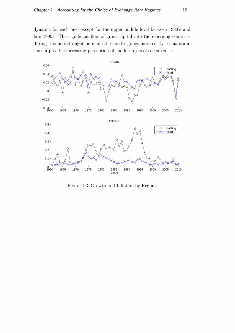
Chapter 1. Accounting for the Choice of Exchange Rate Regimes 18
dynamic for each one, except for the upper middle level between 1980’s and
late 1990’s. The significant flow of gross capital into the emerging countries
during this period might be made the fixed regimes more costly to maintain,
since a possible increasing perception of sudden reversals occurrence.
1960 1965 1970 1975 1980 1985 1990 1995 2000 2005 2010−0.04
−0.02
0
0.02
0.04
0.06Growth
FloatingFixed
1960 1965 1970 1975 1980 1985 1990 1995 2000 2005 20100
0.1
0.2
0.3
0.4
0.5Inflation
Years
FloatingFixed
Figure 1.3: Growth and Inflation by Regime

Chapter 1. Accounting for the Choice of Exchange Rate Regimes 19
1960 1965 1970 1975 1980 1985 1990 1995 2000 2005 20100
0.1
0.2
0.3
0.4
0.5
0.6
0.7
Years
Cou
ntrie
s pr
opor
tion
on F
loat
ing
LowLow MiddleUpper MiddleHigh
Figure 1.4: Floating Regime by Income
1.3Model
We adapt from Buera et al. (2011) and propose an economy in which the
policymaker does not know exactly how the exchange rate regime (henceforth,
ERR) impacts growth and inflation. Instead, he is in constant learning,
whenever new data is available to him. In fact, the policymaker observes
the recent history of ERR impacting growth and inflation of every country
and then shapes his belief of the impact on his country. The data arrives
with uncertainty, which is directly proportional to the country’s distance from
where the information comes from. For instance, a Brazilian policymaker would
be less skeptical about information relating ERR and growth (and inflation)
coming from Argentine than from China. Moreover, a known cost of adopting
the float ERR is also considered, which arises from restrictions on related
economic variables. For instance, with other things the same, managing the
currency demands a high level of international reserves, so, having it decreases
the cost of floating regime.
Specifically, the policymaker is in power for one period and must choose
between floating and fixed ERR. Let θn,t be a period t indicator variable that
equals one if the policymaker of country n chooses floating and equals zero
otherwise. With the purpose of analyzing individual driving forces on choices,

Chapter 1. Accounting for the Choice of Exchange Rate Regimes 20
we rely upon three specifications for policy function. In the first one, the
policymaker cares only about growth, while in the second one, the policymaker
cares only about inflation. Finally, in the more general specification, the
policymaker cares about both variables, weighing each of them into the
function. Specifically, the general period t objective function of the policymaker
of country n is
En,t−1
[I(m∈1,3)yn,t + aI(m∈2,3)πn,t − θn,tKn,t...
−ϕF (θn,t − θn,t−1) θn,t + ϕP (θn,t − θn,t−1) (1− θn,t)
](1-1)
where I(m∈j,k) is an indicator function for the j-th and k-th specification of
the policy function, yn,t is the period t growth rate of the per capita GDP of
country n, a is the relative weight on inflation, πn,t is the period t inflation
rate of country n, Kn,t is the period t floating ERR cost of country n, ϕF
is the switching cost from fixed to floating regime and ϕP is the switching
cost from floating to fixed regime. So, the policymaker considers growth and
inflation, either separately or weighted in according to the specification, but
always considering the cost in adopting the floating regime and the cost of
switching between the arrangements.
As aforementioned, the regime’s choices are restricted by domestic
variables. For instance, with other things the same, it is unlikely to pursue
a fixed regime indefinitely with scarce international reserves. Therefore, low
international reserves must be an encouraging factor toward a floating regime.
To deal with this, we assume a cost of adopting the floating regime, defined
by Kn,t, which is a linear function of a country specific term fn , a period t
vector Πn,t of observable economic variables related to regimes’ choice (such as
international reserves, external debt, gdp per capita) plus an error term kn,t.
That is,
Kn,t ≡ fn + ξ′Πn,t + kn,t, (1-2)
where kn,ti.i.d∼ N (0, %2
n).
We follow Buera et al. (2011) and assume each policymaker as having a
perceived relation between growth and regimes. Additionally, we also propose
a similar policymaker’s beliefs on inflation and regimes. Specifically, for each
country n, we have
Xn,t = Bn,tΘn,t + εn,t, (1-3)
where Xn,t =
[yn,t
πn,t
], Bn,t =
[βy,Fn,t βy,Pn,t
βπ,Fn,t βπ,Pt π∗t−1
],Θn,t =
[θt
1− θt
], εn,t =

Chapter 1. Accounting for the Choice of Exchange Rate Regimes 21
[εyn,t
επn,t
], βy,Fn,t and βy,Pn,t are the period t perceived economic growth under
floating and fixed ERR, respectively, βπ,Fn,t is the period t perceived inflation
under floating ERR , βπ,Pt is the period t proportion in which the inflation
pegs to a target inflation under fixed ERR, π∗t is the period t target inflation
in which we assume being the period t − 1 US inflation, εyn,ti.i.d∼ N
(0,Σy
n,t
)and επn,t
i.i.d∼ N(0,Σπ
n,t
). So, in each period t, the policymaker of country n
has different beliefs (βy,Fn,t and βy,Pn,t ) about how regimes impact growth and
he believes that inflation will be βπ,Fn,t if he adopts the floating regime and a
proportion βπ,Ft of the last period US inflation if he adopts the fixed regime. We
rely on this last feature to avoid additional (in fact, n) parameters within the
model, since it already may suffer from possible overparameterization problem.
Furthermore, when a policymaker pegs its currency, somehow he is trying to
import monetary credibility from a country with low inflation, as the United
States. So, usually, the currencies are pegged to the American Dollar. Thus,
we see as appropriate to assume the country inflation moving toward the US
inflation when the fixed regime is adopted.
The uncertainty arises since the policymaker lacks knowledge of real
values of βy,Pn,t , βy,Fn,t , βπ,Fn,t and βπ,Pt . Instead, he makes inference about their
distributions whenever new information arrives in each period. Particularly,
at the end of period t − 1, the policymaker observes the relation between
ERR choices and growth and inflation from all countries and updates his
beliefs about βy,Pn,t , βy,Fn,t , βπ,Fn,t and βπ,Pt . Lastly, at the beginning of period
t, he observes the realization of the floating cost and, with knowledge of ϕF
and ϕP , he chooses the ERR to foster. The learning procedure is obtained
by application of recursive estimation of weighted least squares in which we
endow the policymakers with Σ, the covariance matrix of a reduced form
model regarding growth, inflation, and exchange rate regimes. See Appendix
for details.
The general problem of the policymaker is to maximize (1-1) constrained
to (1-2) and (1-3), obeying the beliefs dynamic of Bn,t. Solving it, we have the
following optimal policy:
θn,t = I[En,t−1(βy,Fn,t +aβπ,Fn,t )−ϕF (1−θn,t−1)>En,t−1(βy,Pn,t +aβπ,Pt π∗t )+Kn,t−ϕP θn,t−1],
where I[·] is the indicator function.
Thus, if the last regime was floating, the policymaker chooses to keep it if
the difference between the expected growth rate and inflation under floating is

Chapter 1. Accounting for the Choice of Exchange Rate Regimes 22
greater than this difference under fixed regime plus the costs of floating ERR
and the switching toward fixed regime. Additionally, if the last regime was
fixed, the policymakers choose to switch to floating if the difference between
the expected growth rate and inflation under floating minus the switching cost
to floating is greater than this difference under fixed regime plus the costs of
floating ERR.
1.4Inference and Results
1.4.1Estimation
The model is estimated by using Bayesian techniques.5 Thus, we
are interested in the posterior density of α ≡[βy,Pn,0
n,βy,Fn,0
n,
βπ,Fn,0
n, βπ,F0 , νynn, νπnn,νπ,P , %nn, ξ, ϕP , ϕF , a,γy, γπ
]. Defining
Dt =[yt, πt, θt,Πt
]≡[yn,tn,πn,tn, θn,tn , Πn,tn
]and DT ≡ DtTt=1,
the application of Bayes’ rule results in p(α|DT
)∝ P
(DT |α
)· p (α), where
p(α|DT
)is the posterior density of α, P
(DT |α
)is likelihood function and
p (α) is the prior density of α.
Exploring the optimal policy6, we obtain the following likelihood
function:
P(θn,t|Πn,t, D
t−1, α)
=Φ
βFn,t−1 − βPn,t−1 − fn + a(βπ,Fn,t − β
π,Pt π∗
t
)− ξ′
Πn,t − ϕF (1− θn,t−1) + ϕP θn,t−1
%n
θn,t
...
...·
1− Φ
βFn,t−1 − βPn,t−1 − fn + a(βπ,Fn,t − β
π,Pt π∗
t
)− ξ′
Πn,t − ϕF (1− θn,t−1) + ϕP θn,t−1
%n
1−θn,t
,
where Φ (·) is the standard Gaussian cumulative distribution.
In addition, we use informative priors to mitigate the
overparameterization problem of the model. Thus, we assume the parameters
as having the following prior distributions:
5The model with no learning can be viewed as standard Probit model. However, inadvance, the estimated parameters strengthening the learning mechanism are statisticallysignificant. Moreover, the incidental parameters problem can arise in estimation of binarynonlinear models with fixed effects, such as the proposed model either encompassing or notthe learning structure.
6See appendix for details.

Chapter 1. Accounting for the Choice of Exchange Rate Regimes 23
βPn,0 ∼ N(βP0 , ω
2β
), n = 1, ..., N,
βFn,0 ∼ N(βF0 , ω
2β
), n = 1, ..., N,
νyn ∼ IG (sν , dν) , n = 1, ..., N,
νπn ∼ IG (sν , dν) , n = 1, ..., N,
νπ,P ∼ IG (sν , dν) ,
%n ∼ IG (s%, d%) , n = 1, ..., N,
fn ∼ N(f , ω2
f
)a ∼ Uniform,
ξ ∼ Uniform,
γk ∼ Uniform, k ∈ y, π .
We set βP0 = 3.05% and βF0 = 2.19% according to pre-sample average
data; ω2β = 0.03 to adopt a skeptical view on βn,0; sν = dν = 0.26 according
to Buera et al. (2011); s% = d% = 0.01 to avoid the model to fit the data using
a large variance in Kn,t; f = 0 to prevent a prior view of how floating cost
impacts choices, on average; and ω2f = 0.02 to also adopt a skeptical view on
fn. Finally, we use flat priors for α, ξ and γk, so every value is equally likely
to all countries.
Finally, the estimate for α is obtained by maximization of the posterior
of the model. Specifically, we have
α = arg maxα
∏j∈J
p (αj)N∏n=1
[P (θn,1|Πn,1, α) ·
T∏t=2
P(θn,t|Πn,t, D
t−1, α)]
,
where αj accounts for the individuals parameters that compose α, J is the set of
all estimated parameters in the model, p (αj) is the prior density of parameter
αj according to above definitions and P (·) is the likelihood function.
We note that the posterior is not necessarily strictly concave. Thus, it
may exist maximization issues in the optimization procedure. To handle this
question, the optimization is performed starting from some different initial
points. Finally, the estimates are the ones that return the maximum posterior
among all maximizers.
Finally, the model is estimated with annual data, ranging from 1970 to
2010 and covering 91 countries. Because of missing data, the total observation
is 2314. As briefly discussed early, the possible overparameterization problem
is mitigated by using priors in the estimation procedure. Data on inflation,

Chapter 1. Accounting for the Choice of Exchange Rate Regimes 24
growth, and other economic variables are extracted from World Bank, while
data on exchange rate choices are extracted from Reinhart e Rogoff (2004).
1.4.2Reduced-form regressions
Before going to structural model results, we run unbalanced panel
regressions to further examine the relationship between ERR, growth, and
inflation. Specifically, we find partial correlations that floating ERR is
negatively correlated with growth and positively correlated with inflation, even
after controlling for other economic variables.
Furthermore, interestingly for our purposes is to capture some
reduced-form evidence of learning in the data. To that end, we also run
unbalanced panel regressions and show that the choice of country to adopt
floating ERR is correlated with the fraction of neighboring countries following
these policies and their past growth and inflation performances.
Specifically, we consider the following model:
θn,t = φ0 + φ1θn,t−1 + φ2En,t−1 (yt|θ = 1) + φ3En,t−1 (yt|θ = 0) + ...
...+ φ4En,t−1 (πt|θ = 1) + φ5En,t−1 (πt|θ = 0) + ΦCn,t,
where En,t (x|θ) ≡∑τs=1
∑j:θj,t−s=θ exp
(−dnjδ
)xn,t−s∑τ
s=1
∑j:θj,t−s=θ exp
(−dnjδ
) captures some effects of
countries beliefs on their choices and Cn,t accounts for economic variables
(reserves, trade, debt and GDP) as controls; we set δ = 2500, which fixes
the effective neighborhood of the median country, defined as∑
j 6=i exp(−dnjδ
),
to be 20 countries and we set τ = 3, allowing three years of historical data in
shaping the countries beliefs. For robustness purposes, we also run the model
setting δ = 500 and τ = 6 and the results do not change significantly.
As our theory argues, we expect φ1 > 0 as a consequence of persistent
belief of the Bayesian learning. Moreover, we also expect that countries are
more prone to adopt floating ERR in periods in which their neighbors which
adopted the same have higher growth and lower inflation, that is φ2 > 0 and
φ4 < 0. Finally, we expect countries less prone to adopt floating ERR in periods
in which their neighbors which adopted the fixed regime have higher growth
and lower inflation, that is φ3 < 0 and φ5 > 0. As we can verify in Table
1.1, we find statistical significance in the reduced-form model evidencing that
countries tend to adopt floating regime when neighbors do the same and have
greater growth and lower inflation, and when neighbors chose to fix and have

Chapter 1. Accounting for the Choice of Exchange Rate Regimes 25
lower growth and higher inflation.
(I) (II) (III) (IV)
φ00.0514
(0.0292)
0.0517
(0.0292)
0.0482
(0.0399)
0.0484
(0.0399)
φ10.8522∗∗∗
(0.0129)
0.8522∗∗∗
(0.0129)
0.8510∗∗∗
(0.0130)
0.8510∗∗∗
(0.0130)
φ21.3553∗∗
(0.3619)
1.3537∗∗
(0.3685)
1.0268∗
(0.4836)
1.0257∗
(0.4842)
φ3−2.6279∗∗
(0.7143)
−2.6335∗∗
(0.7438)
−1.8740
(1.1062)
−1.8740
(1.1082)
φ4−0.0028
(0.0022)
−0.0028
(0.0022)
−0.0050
(0.0029)
−0.0049
(0.0029)
φ50.0078∗∗∗
(0.0022)
0.0078∗∗∗
(0.0022)
0.0089∗∗
(0.0029)
0.0089∗
(0.0029)
Reserves−0.0967
(0.0216)
−0.0966
(0.0216)
−0.0939
(0.0215)
−0.0939
(0.0215)
Trade0.7171
(0.3889)
0.7195
(0.3891)
0.7473
(0.3861)
0.7480
(0.3860)
Debt Service0.0007
(0.0011)
0.0007
(0.0009)
0.0008
(0.0011)
0.00010
(0.0010)
GDP per capita3.2488∗
(1.6307)
3.2495∗
(1.6302)
3.2106∗
(1.6487)
3.2030∗
(1.6480)
δ 2500 500 2500 500
τ 3 3 6 6∗,∗∗and ∗∗∗ mean significant at 5%, 1% and 0.1% respectively.
Table 1.1: Reduced form results with “learning”
1.4.3Semi-structural Models
Now we turn to the results of the semi-structural models. Table
1.2 reports the point estimates of the parameters with standard errors in
parenthesis. As we can see, we find no statistical significance for the parameter
weighting the inflation on policy function, besides having a positive sign. So,
the policymaker would give more value to high inflation, a non-intuitive result.
One possible explanation lies in the fact that we use data containing only

Chapter 1. Accounting for the Choice of Exchange Rate Regimes 26
countries with inflation lower than 50% per year7, ruling out countries which
suffered from hyperinflation, those in which the most would take advantage
of choosing the exchange rate regime when fostering low inflation. Moreover,
in last decades, other nominal anchors are adopted by countries in controlling
inflation, such as an inflation target.
The results also report that prior belief of the cross-country correlation
decreases with geographic distance, since the coefficient λ is positive. This
has an intuitive interpretation: in the learning process, the policymaker gives
more weight to observed relationship between regimes and growth in closer
countries. For example, a Brazilian policymaker is less uncertain about how this
relationship in Argentina could be related to his country than this relationship
in China.
Regarding floating costs, the results suggest that the larger
reserves,Regarding floating costs, the results suggest that the larger reserves,
the higher the cost of floating exchange rate regime. In other words, the
policymaker tends to choose a fixed regime when the reserves are high. An
intuitive result, since high reserves help to lessen the probability of currency
attackIn fact, managing exchange rate demands a high level of foreign
currency., generating an auspicious environment for fixed regime. This finding
is consistent with the early reported IMF’s concerns about the arrangements.
7We do that because of technical issues. Very high inflation cause misbehavior in theoptimization procedure, specifically, the Σ acquires unstable values.

Chapter 1. Accounting for the Choice of Exchange Rate Regimes 27
Description Specification I Spec. II Spec. III
Inflation Weighting
a weight on inflation0.0115
(0.0074)- 1
Prior Correlation
γy geographic distance (growth)0.0082
(0.0039)
0.0516
(0.0178)-
γπ geographic distance (inflation)0.0022
(0.039)-
2.5771
(0.6916)
Floating Costs
ξ1 reserves over GDP0.0203
(0.0098)
0.1366
(0.0524)
0.1664
(0.0855)
ξ2 debt services over GDP−0.0005
(0.0001)
−0.0026
(0.0048)
−0.0021
(0.0032)
ξ3 relative GDP per capita0.7727
(0.5222)
−0.3156
(0.2246)
−0.5487
(0.2310)
ξ4 trade over GDP−0.0101
(0.0029)
0.0012
(0.0936)
0.0576
(0.0528)
Switching Costs
ϕP cost from floating to fixed regime0.0096
(0.0034)
0.0324
(0.0445)
0.0483
(0.0310)
ϕF cost from fixed to floating regime0.0042
(0.0034)
0.0420
(0.0377)
0.0542
(0.0330)
Table 1.2: Estimation Results
With respect to debt services, the model reports a slight evidence
this variable encouraging floating regime, with the interpretation relying on
credibility issues. Besides the reserves, the policymaker can also use the
interest rate as a tool to peg his currency to another. However, if the country
lacks credibility in maintaining the fixed regime, the international market will
request increasing interest rate to offset an expected depreciation. But, existing
internal issues limits the increase in interest rate, such as unemployment.8 So,
a country with high debt must stay prone to choose a floating regime. A similar
interpretation is pointed by Bleaney e Ozkan (2011), in which the authors
claim that the perceived likelihood of using an“escape clause” in pegged regime
raises its adoption cost.
The results evidence a negative impact of GDP per capita on floating
choice. Views related to political economy are more appropriate to interpret
it. Governments fostering low inflation, but also showing low institutional
8For example, the Brazil undervaluation in 1999.

Chapter 1. Accounting for the Choice of Exchange Rate Regimes 28
credibility, may adopt fixed regime to tame inflationary expectations, unlike
countries with high institutional quality. It follows that the formers are more
prone to foster a fixed regime, while the latter may embrace a floating regime.
These results are in agreement with Levy Yeyati et al. (2010). Regarding trade,
we find a negative estimate, evidencing that trade discourages floating regime,
as expected. When it comes to the switching cost, we see evidence of positive
cost for both, from fixed to floating and from floating to fixed, but only the
latter is statistically significant.
1970 1975 1980 1985 1990 1995 2000 2005 20100
0.05
0.1
0.15
0.2
0.25
Model’s Fit
Figure 1.5: Model’s Fit
Figure 1.5 reports the model’s ability in fitting the observed data. The
predicted series corresponds to the one-step-ahead prediction with no shock to
the floating ERR. As we can see, the predicted data is able to match fairly well
the observed data. In addition, the model predicts 96.4% of the observed policy
choices. However, these results must be interpreted with caveats. Additional
analysis is requested to assess potential overparameterization problem, since a
large number of estimated parameters in the sample. Future works encompass
out-of-sample forecasting and a better understanding of learning rule in
prediction. Lastly, we also turn off the learning mechanism9 and the estimates
do not change significantly, as well as the prediction rate, which falls marginally
to 95.9%.
However, when predicting policy switches, the learning mechanism gain
a prominent rule. While the no learning model is unable to predict any regime
switch within a one-year window, on the other hand, when encompassing the
9Specifically, we let Ψt = Ψ0 and Pt = P0, ∀t.

Chapter 1. Accounting for the Choice of Exchange Rate Regimes 29
learning mechanism, the model forecasts 14% of the switches. So, the learning
dynamic is essential to predict policy switches
Lastly, figures 1.6 and 1.7 report the model generated beliefs for growth
and inflation, respectively, for each country according to their choices, with
the bold line accounting for median values. As we can see in the former, in the
median, the growth belief if fixed is greater than growth belief if floating, with
both decreasing along years. In the latter, a falling tendency in inflation if fixed
is observed, while the opposite movement is verified in inflation if floating.
1970 1980 1990 2000 2010−0.1
−0.08
−0.06
−0.04
−0.02
0
0.02
0.04
0.06
0.08
0.1Growth Belief if Fixed
1970 1980 1990 2000 2010−0.1
−0.08
−0.06
−0.04
−0.02
0
0.02
0.04
0.06
0.08
0.1Growth Belief if Floating
Figure 1.6: Growth Beliefs
1970 1980 1990 2000 20100
0.05
0.1
0.15
0.2
0.25
Inflation Belief if Fixed
1970 1980 1990 2000 20100
0.05
0.1
0.15
0.2
0.25
Inflation Belief if Floating
Figure 1.7: Inflation Beliefs

Chapter 1. Accounting for the Choice of Exchange Rate Regimes 30
1.5Conclusion
The paper analyzes how countries choose their exchange rate regime,
whether to fix or to float. We explore the lack of consensus on it and propose
a model in which the policymaker learns how the regimes impact growth
and inflation. Additional to the learning process, relevant economic variables
related to an open economy are also considered on choices, as well as costs of
switching between regimes.
The model was estimated by Bayesian techniques and we find results
suggesting intuitive connections between economic variables and choices.
Specifically, the results evidence that higher reserves encourage fixed regime,
while higher debt service and GDP per capita encourage floating regime.
Moreover, we find evidence of positive switching costs, but statistically
significant only from floating to pegged. Lastly, we find no evidence that the
policymaker considers inflation in his choice. In fact, fixed regime usually is
used to strongly disinflate the economy, while conventional monetary tools
are requested to maintain an environment with low inflation. Since, for
computational purposes, we have discarded hyperinflation cases, the data
encompass only the latter scenario. Finally, as a drawback, the model can suffer
from potential overparameterization problem, which we tried to mitigate using
priors within the Bayesian scheme.

2A Model For Household Inflation Expectations
2.1Introduction
The paper models how households form inflation expectations. To do so,
we suggest an environment in which, when forecasting future inflation, the
household relies on two informational sources. On one hand, he can derive
his inflation prediction from the expectations of professionals, which could be
assimilated from economic news reported by the media. On the other, the
inflation predicted by a typical person will be one to be replicated by a simple
econometric model encompassing a learning structure. As we will see, the
learning mechanism plays a major role when discounting past data to predict
future inflation, mainly in countries with a history of hyperinflation, just as the
Brazilian case. The switches between the alternatives are time-varying, based
on characteristics of the sources, such as the historical success in matching
past inflation, and on characteristics of the individuals, such as the capacity in
assimilating news. Because of the individual characteristics, not all households
are guided by the same informational source. So, the mean household inflation
expectations is a weighted average considering the ratio of households guided
by each informational sources.
Inflation expectations assume a key role in monetary policy, mainly in
those countries in which the central bank is committed to price stability.
The intuition is straightforward and follows the New Keynesian theory: when
planning his optimal consumption choices, the consumer must consider the
expected economic conditions that will prevail, including future prices. Thus,
inflation expectations influence actual consumption and, as a consequence, the
price index to be controlled by the monetary authority. So, how agents form
inflation expectations becomes an important matter for policymaker’s issues.
Since the work of Muth (1961) and Lucas (1972), the benchmark
theoretical model of expectations’ formation in economics has been the
rational expectations theory, which advocates agent expectations being the
true statistical conditional expectation of the variables in the economy.
However, this demand for complex knowledge of the world has generated
several criticisms on theory, mainly focused on its inadequacy in accounting
for real process of economic forecasting. In that way, some works find
evidence against rational expectations hypothesis when compared with survey

Chapter 2. A Model For Household Inflation Expectations 32
expectations.1 Therefore, as shown by Bernanke (2007), while the rational
expectations theory is helpful for some specific analysis, it might be less
effective within an environment in which people know imperfectly the structure
of the economy which constantly evolves over time and the private sector lacks
full understanding of the policymaker behavior. The Bernanke’s criticism is
even more valuable when dealing with ordinary people shaping expectations,
as in our case.
As a consequence, in the last decade, an increasing number of studies
addressing how agents form expectations has gained ground in the literature.
Many of them are based on informational frictions.2 In this way, Sims (2003)
elaborates the rational inattention theory, in which ”to pay attention” incurs a
cost to the agent, since he has a finite capacity to process all information
that surrounds him. Thus, this scarcity on cognitive capacities forces the
agent to select what is worth for him to pay more, or less, attention to.
In addition, Mankiw e Reis (2002) propose a sticky information expectations
encompassing a slow dispersal of information among the people regarding
macroeconomic conditions. While Mankiw e Reis (2002)’s model accounts for
expectations’ formation of a general agent, Carroll (2003) is the first one to
suggest how household forms expectations on inflation. The author proposes an
epidemiological expectations model in which a fixed proportion of households
forms inflation expectations when observing the views of professionals reported
by the media, while the complementary proportion uses his last predicted
value. The work of Lanne et al. (2009) also must be highlighted, in which the
authors slightly modify Carroll’s model, allowing the household to replicate
the last realized inflation instead of professional’s view as an alternative to
last predicted value when predicting future inflation.
Another growing branch in the literature of expectations’ formation is
the learning theory, based on the principle of cognitive consistency theory.3
The theory assumes the agent behaving as an econometrician, so economic
variables are forecast by using of time-series econometric techniques. One of
the interesting features in the learning procedure is the possibility to adjust
the agent’s information set and parameters according to his knowledge of the
economy. For instance, Branch e Evans (2006), when modeling professional
inflation expectations, use an adaptive learning procedure in which inflation
and output are present in the agent’s information set. In advance, we use
1See Pesaran e Weale (2006) for discussion on that.2See e.g. Mankiw e Reis (2002); Carroll (2003); Sims (2003); Reis (2006), Reis (2006)
and Lanne et al. (2009).3See Evans e Honkapohja (2001) for an overview of learning on economics and e.g.
Branch (2004), Branch (2007); Branch e Evans (2006); Orphanides e Williams (2008) andEasaw e Mossay (2015) for applications of learning on expectations formation.

Chapter 2. A Model For Household Inflation Expectations 33
only inflation in the information set of the household when partially modeling
his inflation expectations. Moreover, Weber (2007) finds that professional uses
higher constant gain parameter in learning algorithm than a household. Thus,
as expected, it seems that the process of updating information is less costly
for the former than for the latter.
As contributing to literature, the proposed model brings together features
of both processes of expectations’ formation when modeling the household
inflation expectations. First, we assume the household with informational
constraints. As we will see, the household derives utility from the observable
historical success, as it being a potential indicator of future success in
predicting the inflation. Nevertheless, he may still be guided by the source
having the worst past success. This is possible since the model also allows
non-observable to affect what source to follow. For instance, the household
may rely on the econometric model even if the professional has better historical
success, because he may not have paid attention to the news. Thus, assimilated
news should be a potential driving force in leaning into the professional’s views,
but not the only, as in Carroll (2003). However, note that assimilating news
from professional’s view does not necessarily imply to be guided by professional
expectations. The household may still be inclined to follow the econometric
model forecast, once again, since it may have better historical success.
Second, the household behaves as an econometrician when not relying
on professional’s views. In the existing literature of how household forms
inflation expectations, when not following the professionals, the household
usually replicates his previous forecast, or he assumes the last realized inflation.
In our case, the household forecast inflation by using a simple linear relation
whenever new data of inflation is available. We model it by adaptive learning
with constant gain, which has a predominant role in discounting past inflation
when forecasting the future one, being crucial in modeling expectations in an
economy which has suffered from hyperinflation, as the Brazilian case. In the
same vein, Malmendier et al. (2016) have also emphasized central implications
of learning from experience when modeling expectations. According to the
authors, the expectations are history-dependent and heterogeneous, with young
people placing more weight on recent data than the older ones. So, this latter
feature is widely suitable for our purposes.
We also analyze the partial correlation between news absorbed by
households and the formation of inflation expectations. In our model, the
spreading news is one of the channels in which the household assimilates
the professional’s views of future inflation.4 So, with other things the same,
4The way in which media influences the people’s views about economic aggregate is well

Chapter 2. A Model For Household Inflation Expectations 34
more news would imply more weight for professional expectations in household
expectations. Thus, we use realized data for the proportion of households
assimilating news of inflation and assess its co-movement with the model
generated data related to the probabilities with which the household chooses
the professional’s view. In fact, we find that household absorbing news has a
positive correlation with his choice for the professional inflation expectations.
Carroll (2003) and Pfajfar e Santoro (2013) analyze the same implication by
considering the impact of news over an observable gap between the prediction
of inflation by household and by professional.
The remainder of the paper is organized as follows. Section 2 describes
the model; Section 3 assesses the model’s fit to the data - emphasizing the
major role of learning mechanism when modeling inflation expectations in an
economy with history of high inflation - and discusses the correlation between
news and the formation of household inflation expectations; Section 4 analyzes
the link between central bank transparency and the formation of inflation
expectations; and, finally, Section 5 concludes the paper.
2.2Economic Environment
We propose an environment in which the household forms expectations
about future inflation based on two alternative sources: from professional
forecasting and from an econometric model forecasting. The professional source
reports the inflation expectations of experts and the household can access it
by various means, including news reported by the media. A similar way of
household absorbing information of inflation is found in Carroll (2003), Easaw
et al. (2010) and Pfajfar et al. (2013). As an alternative to the professional
source, the household predicts future inflation on his own, which we assume
to follow a simple econometric model, encompassing an adaptive learning
structure. So, the household updates his inflation forecast as soon as new
data on inflation is available. Branch et al. (2006) use a resembling learning
structure, but with wider information set, to analyze how professional shapes
inflation expectations.
The switches between the alternatives take into account observables
related to the sources, such as historical success in matching past inflation, and
non-observables related to characteristics of each household, such as propensity
to assimilate the news from media.5 Because of individual characteristics, in
each period, not all households are guided by the same informational source.
documented in Blinder and Krueguer (2004)5Another means would be word to mouth. In this case, one household would absorb the
news, or even predict as professional, and pass through to others.

Chapter 2. A Model For Household Inflation Expectations 35
Thus, the final household inflation expectations is a weighted mean considering
the likelihood of the household relying on each alternative of information.6
In contrast to Carroll (2003), the household considers the (time-varying)
observable historical success of alternatives when choosing, so the assimilated
news do not assume the unique role that dictates the source to follow.
Specifically, let yt be the information source chosen by the household in
period t, let j ∈ P,M denote the alternative source of information with P for
“professional” source and M for “econometric model” source, let Xt be a vector
with period t historical success in match past inflation of alternatives7 and let
at be a vector of unobservable variables affecting households’ tastes of each
alternative. For example, the vector a may contain the news assimilated by
household, the only channel in which the household chooses the professional’s
views in Carroll (2003). In addition, consider a situation in which, in each
period t, the household obtains information of future inflation from professional
expectations with probability P (yt = P |Xt, at), while he obtains information
of future inflation from his own forecast, which we assume to follow an
econometric model, with probability P (yt = M |Xt, at). Then, the period t
population mean of household inflation expectations given the information set
in t− 1 is
πHt|t−1 = P (yt = P |Xt, at) πPt|t−1 + P (yt = M |Xt, at) π
Mt|t−1, (2-1)
where πPt|t−1 is the professional inflation expectation for period t given the
information set in t−1 and πMt|t−1 is the econometric model inflation forecasting
for period t given the information set in t− 1.
Unlike Carroll (2003), we allow the probability of relying on the
information sources to vary along time. For instance, the household must be
more prone to lean into the professional source since it successfully matched
the last inflations, or still he may be more likely to absorb news in some
period. In turn, the absorbing news may be related to non-observable data,
such as increasing household reading skills, decreasing newspaper price, more
spreading media information and so on. In addition, the non-observable data
can also include the tones of news reported in media, since not only the amount
of news matters for expectations formation, but also their tone, as exposed by
Soroka (2006) and Hamilton (2004). An analogous analysis can be made when
household relies on econometric model source.
6We can also assume the economy composed of a continuum of agents of measure one,in which a proportion p relies on one source, and the complement 1 − p relies on anothersource.
7In advance, we define historical success as the negative of mean square error betweenthe last four quarters of realized inflation and the alternative forecasts

Chapter 2. A Model For Household Inflation Expectations 36
Specifically, let Ut,j be the period t household’s utility when choosing
source j that depends of the observable and non-observable variables of the
alternatives. Following that, we assume
Ut,j = Xt,jω + at,
where ω is a parameter to be estimated and the others variables are as definied
before.
As a rational agent, the household chooses yt = j ∈ P,M which
maximizes his utility, that is,
yt = argmaxP,M
(Ut,P , Ut,M) .
Since yt is the maximizer choice, we set at,j to be Gumbel independently
distributed.8 Then, as showed by McFadden (1974),
P (yt = j|Xt) =exp (Xt,jω)
exp (Xt,Pω) + exp (Xt,Mω), j ∈ P,M . (2-2)
So, with all else unchanged, the higher the historical success of a source,
the greater the probability of household to rely on it. The parameter ω
accounts for intensity of choice when the elements in Xt differs. For example,
if ω → ∞ and Xt,P differs positively from Xt,M in an infinitesimal amount,
then P (yt = P |Xt) = 1. On the other hand, if ω = 0, then P (yt = P |Xt) =
P (yt = M |Xt) = 0.5 whatever the difference between the elements in Xt.
Somehow, the ω can also be seen as a parameter for “inattentiveness level”.
The equation 2-2 is usually called as conditional logit equation.
When the household does not rely on professional’s views of inflation,
he predicts it from his own, which we assume to follow an econometric
model. This model must be as simple as possible to reflect the limited
household’s knowledge about the economy and also must incorporate the
economy’s structure changing over time, as pointed by Stock e Watson (2003),
Cogley e Sargent (2005), Sims e Zha (2006) and Sargent et al. (2006). Under
those circumstances, the econometric model follows a learning structure for
inflation forecasting.9 The learning literature has gained ground in modeling
agents’ expectations in economics. For example, Branch e Evans (2006),
Easaw e Golinelli (2010) and Malmendier e Nagel (2016) model inflation
expectations using a learning mechanism.
8The Gumbel distribution is also known as type I extreme value distribution, a particularcase of the generalized extreme value distributions.
9Some works suggest that household keeps his last forecast when not absorbing theprofessional’s, as Carroll (2003), Lanne et al. (2009) and Easaw et al. (2013).
Chapter 2. A Model For Household Inflation Expectations 37
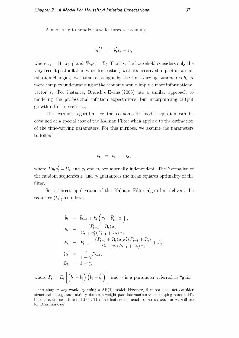
A mere way to handle those features is assuming
πMt = b′
txt + εt,
where xt = [1 πt−1] and Eεtε′t = Σt. That is, the household considers only the
very recent past inflation when forecasting, with its perceived impact on actual
inflation changing over time, as caught by the time-varying parameters bt. A
more complex understanding of the economy would imply a more informational
vector xt. For instance, Branch e Evans (2006) use a similar approach to
modeling the professional inflation expectations, but incorporating output
growth into the vector xt.
The learning algorithm for the econometric model equation can be
obtained as a special case of the Kalman Filter when applied to the estimation
of the time-varying parameters. For this purpose, we assume the parameters
to follow
bt = bt−1 + ηt,
where Eηtη′t = Ωt and εt and ηt are mutually independent. The Normality of
the random sequences εt and ηt guarantees the mean squares optimality of the
filter.10
So, a direct application of the Kalman Filter algorithm delivers the
sequence (bt)t as follows
bt = bt−1 + kt
(πt − b′t−1xt
),
kt =(Pt−1 + Ωt)xt
Σt + x′t (Pt−1 + Ωt)xt,
Pt = Pt−1 −(Pt−1 + Ωt)xtx
′t (Pt−1 + Ωt)
Σt + x′t (Pt−1 + Ωt)xt+ Ωt,
Ωt =γ
1− γPt−1,
Σt = 1− γ,
where Pt = Et
[(bt − bt
)(bt − bt
)′]and γ is a parameter referred as “gain”.
10A simpler way would by using a AR(1) model. However, that one does not considerstructural change and, mainly, does not weight past information when shaping household’sbeliefs regarding future inflation. This last feature is crucial for our purpose, as we will seefor Brazilian case.

Chapter 2. A Model For Household Inflation Expectations 38
If γ = 0, the model is simply a recursive formulation of ordinary least squares,
known in learning literature as Recursive Least Squares (RLS). If γ ∈ (0, 1) ,
the past observations are discounted at geometric rate, and the model is known
in learning literature as Constant Gain Least Squares (CGLS).
Once obtained the sequence(bt
), the forecast inflation of the econometric
model is
πMt|t−1 = b′t−1xt. (2-3)
Therefore, the system composed of equations (2-1)-(2-3) and the
professional’s views of future inflation allow us to set up the household inflation
expectations.
2.3Model’s Analysis
In this section, we analyze empirically the model, in addition to address
the prominent role played by the learning mechanism when forecasting inflation
in an economy with hyperinflation history. First of all, the analysis needs data
of the household inflation expectations, professional inflation expectations and
realized inflation. Then, we are able to assess the model’s fit and compare it
with others in literature. Besides, we also analyze the co-movement between
news and the probabilities in which the household chooses the professional’s
views.
2.3.1Data
For data on household inflation expectations, we rely on Michigan
Survey of Consumers (henceforth, MSC), conducted by the University of
Michigan and Thompson Reuters. The survey is nationally representative and
interviews approximately 500 households per month. Among the questions,
the respondents are asked about their expected inflation rate for the next
twelve months in a numerical value. The question is as follows: “By about
what percent do you expect prices to go (up/down) on the average, during the
next 12 months?”
In order to mitigate possibles outliers, we focus on median answers.
The survey shows large heterogeneity between respondents. In fact, there are
some households expecting extreme inflation, as we can see in Figure 2.1.
A possible explanation for that lies behind the non-uniformity price changes
across products. When asked about price change, the household may give a
wider weight on a specific product in his consumption basket, generally, the

Chapter 2. A Model For Household Inflation Expectations 39
one that most changed, as pointed by Ranyard et al. (2008). Moreover, the
household may not have a adequate interpretation about the question, since the
word “inflation” is not used. In accordance with Bruine de Bruin et al. (2010),
some respondent can interpret it as a question about his personal expenses and
report a more extreme inflation expectations. This fact is evidenced in Figure
2.2, which plots the mean and median households’ answers to the survey, with
the former higher than the latter for every period.
2000 2001 2002 2003 2004 2005 2006 2007 2008 2009 2010 2011 2012 20130
10
20
30
40
50
60
DownSameUp by 1−2%Up by 3−4%Up by 5% or moreUp but don’t knowDon’t Know
Figure 2.1: Yearly average proportions answers.
1980 1985 1990 1995 2000 2005 20100
2
4
6
8
10
12
14
MedianMean
Figure 2.2: Household inflation expectations
For data on professional inflation expectations, we rely on Survey of
Professional Forecasters (henceforth, SPF), conducted from 1968 to 1992 by
American Statistical Association and National Bureau of Economic Research

Chapter 2. A Model For Household Inflation Expectations 40
and since then by Federal Reserve Bank of Philadelphia. The survey’s
questionnaire is delivered quarterly to professional forecasters, asking them
about future inflation, among other variables. Specifically, the respondents are
questioned for their forecasts for the next four quarters on Consumer Price
Index (CPI) inflation. Since mean and median answers from professionals do
not present any bias, we focus on the mean one.
Lastly, for realized inflation, we use the “Consumer Price Index for All
Urban Consumers: All Items” available by US Bureau of Labor Statistics.
This data is built upon the average monthly change in the price for goods
and services bought by urban consumers, and represents the buying habits of
households.
2.3.2Fitting
We now test the model’s ability to adjust to the observed data. The
fitting is analyzed by using quarterly series ranging from 1985Q1 to 2014Q1.
In the learning mechanism, we use a pre-sample estimation for Kalman Filter
initialization. In addition, we set γ = 0.0138 and ω = 0.0521 in order to
minimize the mean squared error between the model generated series and
the observed household inflation expectations The calibrated constant gain
parameter is similar to those found in Orphanides e Williams (2005)2008,
Milani (2007) and Malmendier e Nagel (2016): 0.02, 0.0183 and 0.0180,
respectively. Finally, we assume the historical success of alternative j as the
negative of mean square error between the last four quarters of realized inflation
and alternative forecasts, that is11
Xt,j = −1
4
4∑s=1
(πt−s − πjt−s|t−s−1
)2
, j ∈ P,M .
Figure 2.3 relates graphically the model’s ability in fitting the observed
household inflation expectations. In our point of view, the proposed model has a
satisfactory success in fitting the data, highlighting the short-term movements.
However, it seems to be exceptions for the years from 1987 to 1992 and 2010
onwards.
The satisfactory result is reinforced when focusing on the individuals’
dynamics of series composing the generated data. Each one follows a
specific and distinct path over time if compared with the household inflation
11We may have a potential inconsistency here. The problem arises since we assume that thehousehold must know the last predictions of both sources, despite he used only one. However,we can think that variable as “proxying” a perceived historical of success. Moreover, we varythe quarters of realized inflation and the results do not change significantly.

Chapter 2. A Model For Household Inflation Expectations 41
expectations, as we note in Figure 2.3. Therefore, the model does not mimic
any individual series, but it is the proposed dynamic combination of them
which provides the good fit into the data.
1990 1995 2000 2005 2010−2
−1
0
1
2
3
4
5
6
7
Household Inflation Expectation (obs)ModelRealized InflationConstant Gain Least SquaresProfessional Inflation Expectation
Figure 2.3: Model’s fit and components
We also compare the proposed model with others. The Table 2.1 reports
the mean squared error between generated and observed data, along with
mean and variance of the related individual data. Focusing on those statistics,
our model’s generated data has a satisfactory fit to the observable data,
performing above the Carroll’s model, but slightly below the one proposed by
Lanne et al. (2009). Moreover, once again, it is noteworthy that the proposed
model is able to keep up with short-term movements of observed household
inflation expectations, as we can note in Figure 2.4. In addition, despite
the marginal lower performance compared to Lanne et al. (2009)’s, our model
brings specific features useful to address two interesting matters: learning and
inflation expectations within a hyperinflation history, and the relationship
between news, household expectations and professional expectations.

Chapter 2. A Model For Household Inflation Expectations 42
RMSE¹ Mean Variance
Household Inflation expectations (obs.) 0 2.9560 0.3216
Model 0.7951 3.0940 0.8886
Carroll (2003) 0.9424 3.1664 0.9092
Lanne et. al (2009) 0.7384 2.9119 0.6886
Recursive Least Squares 1.0026 2.9175 1.5711
¹ Relative to observable of household inflation expectations.
Table 2.1: Models’ statistics (USA)
1990 1995 2000 2005 20100
1
2
3
4
5
6
Household Inflation Expectation (obs)ModelCarrol (2003)Lanne et al. (2009)
Figure 2.4: Alternatives models
2.3.3Learning mechanism and hyperinflation history
The learning mechanism acquires major role in modeling the household
inflation expectations in an economy with a record of high inflation, since
it allows the consumers to discount past inflation to forecast the future
one. It follows Malmendier e Nagel (2016), which argue that expectations
are history-dependent and heterogeneous, with young people placing more
weight on recent data than the older ones. So, individuals’ personal
experiences are relevant in shaping their expectations. In similar way, As
a consequence to our purposes, while for the US economy, with no history
of hyperinflation, the proposed model performs marginally below the one
proposed by Lanne et al. (2009), for the Brazilian economy, the former

Chapter 2. A Model For Household Inflation Expectations 43
overcomes significantly the latter, largely due to the adaptive learning
mechanism, as we will see below.
To assess it, we use the aforementioned methodology and address the
same analysis of the Brazilian economy, which has suffered from hyperinflation
in the 1980’s until 1995. Specifically, we explore the fact that there also
exists a series of observed Brazilian consumer inflation expectations, computed
by IBRE/FGV in the same vein of the Michigan Survey. The Figure 2.5a
reports the realized inflation and the consumer expectations. As we can see,
the consumer expectations have a positive bias, mainly if compared with the
professional expectations. This may be due to a high inflation period that
might cause an “inflationary memory” in the consumer expectations. If we use
a simple model of adaptive expectations, such as an auto-regressive one, as
an alternative to following the professional’s view, a pure memory inflationary
emerges for household inflation expectations, as exposed in Figure 2.5b. So,
the early argued adaptive learning model acquires importance in weight past
inflation when the households are forecasting the future one.

Chapter 2. A Model For Household Inflation Expectations 44
2006 2008 2010 2012 2014 20162
3
4
5
6
7
8
9
(a)
RealizedConsumer Expectations (obs)Professional Expectations
2006 2008 2010 2012 2014 20160
2
4
6
8
10
12
14
16
18
20
(b)
RealizedConsumer ExpectationsModel with AR(1)Simple AR(1)
Figure 2.5: Brazilian inflation expectations
In order to estimate the adaptive learning model, we use IPCA (the
official Brazilian inflation index) data ranging from January of 1981 until
February of 2015. For professional expectations, we use data from Central
Bank of Brazil with professional inflation expectations for twelve months ahead
ranging from January of 2004 until December of 2014. The learning parameter
was estimated in γBR = 0.0101 in a monthly frequency, against γUS = 0.0138
in a quarterly frequency for the US, implying that Brazilian consumers use
8.2 years of inflation data while Americans use 18.1 years. We interpret it as
resulting from the fact that Brazilian economy was subject to more frequent
structural breaks, with the ending of the high period inflation being the most
important for our results. Moreover, the parameter accounting for intensity
of choice is estimated in ωBR = 0.0013, while for the US we estimated in
ωUS = 0.0487. So, it seems that American consumers are more sensible to the

Chapter 2. A Model For Household Inflation Expectations 45
difference of historical success between the learning model forecasting and the
professional expectations.
Figure 2.6 reports the model’s fit compared to the Carroll’s and to the
Lanne et al. (2009)’s models. Once again, we are satisfied with the adjust of the
model to the observed data, in which we see the learning mechanism playing
a crucial role. As we can note, unlike for the US economy, the proposed model
has a significantly better performance if compared with the alternatives when
fitting the expectations. We see the improvement as resulting from the fact that
the proposed model allows the Brazilian consumers to discount past inflation
when forecasting the future one, emphasizing the importance of learning in
shaping their expectations. Lastly, Table 2.2 reports some models’ statistics,
reinforcing the better performance of the model encompassing the learning
structure when compared to the others.
1990 1995 2000 2005 20100
1
2
3
4
5
6
Household Inflation Expectation (obs)ModelCarrol (2003)Lanne et al. (2009)
Figure 2.6: Proposed model and alternatives
RMSE¹ Mean Variance
Household Inflation expectations (obs.) 0 6.4882 0.3689
Model 0.3700 6.5076 0.8886
Carroll (2003) 1.5738 5.0742 0.5117
Lanne et. al (2009) 1.6725 5.2626 0.9847
Recursive Least Squares 1.9733 8.2741 1.0899
¹ Relative to observable of household inflation expectations.
Table 2.2: Models’ statistics (BRA)

Chapter 2. A Model For Household Inflation Expectations 46
2.3.4News, household expectations and professional’s view
According to the model, the household can assimilate professional
inflation expectations when in contact with several means of communication.
So, with other things the same, more news heard by households would imply
more choices on professional’s view. Since the model can generate the choice’s
probabilities, we have an intuitive and direct manner to assess the co-movement
between news and the formation of household inflation expectations, something
missing in the other models. Just for reminding, the alternative models assume
as sticky the ratio of households leaning into the professional’s view.
How the media influences the formation of public expectations is deeply
analyzed by Blinder and Krueguer (2004). The authors use a specially-designed
survey and find that large majority of Americans citizens wants to be well
informed about economic issues, with the television and newspapers being their
preferred source of information.12 In light of these findings, Carroll (2003) and
Pfajfar e Santoro (2013) examine the relationship between news and household
inflation expectations using the square of the gap between the Michigan Survey
of Consumers’ and Survey of Professional Forecasters’ predictions as a measure
for“household behaving as professional”. So, the greater amount of news would
imply a shorter gap. However, in our view, this measure may be misspecified in
capturing the impact of news on household’s choice. For instance, in a country
with well-anchored inflation expectations, even if the household does not choose
to follow the professionals, both expectations will still be closer. Therefore, we
see choice’s probabilities on professional expectations as a more appropriate
variable for measuring the impact of news on household expectations.
In order to circumvent this matter, we assess the co-movement of news
with our generated choice’s probabilities on professional expectations, instead
of the gap measure. So, as in Pfajfar e Santoro (2013), we explore the fact
that MSC also asks households if they have heard news about recent changes
in prices. Specifically, the following question is addressed: “During the last
few months, have you heard of any favorable or unfavorable in business
conditions?”. If so, the interviewer asks the second question, “What did you
hear?”, and shows a list of options regarding business conditions, including
prices, that the household might have heard about. Finally, we use the
proportion of the survey’s respondents who had heard about inflation as the
variable related to amount of news on inflation assimilated by the households.
12Nowadays, the Internet must be a key source of information for the general public.

Chapter 2. A Model For Household Inflation Expectations 47
1990 1995 2000 2005 20100
0.5
1
1990 1995 2000 2005 20100
20
40Choice’s Probabilities (left axis)News on Inflation (right axis)
Figure 2.7: Choice’s probabilities and news
Figure 2.7 reports choice’s probabilities on professional expectations and
news absorbed by households. On average, the household chooses professional
expectations in 55% of cases, differently from the 36% of Carroll’s results
and from the 28% of Pfajfar e Santoro (2013)’s. A possible explanation lies
on the better performance by professionals in forecasting the inflation.13
In this sense, while in our model the household must choose between the
econometric model and the professional one, in the others, the selection is
between the actual professional’s forecasting and the last model’s forecasting,
with the latter including a proportion of the last professional’s forecasting.
Since quarterly inflation presents persistence (Cogley e Sargent (2002)), the
last model’s forecasting may be more informative about actual inflation that
the actual econometric model of households. Therefore, if the household
considers the historical success of the alternatives in his choices, he will give
a more weight on professional’s forecasting in our case than in others. Indeed,
we find a positive correlation of 0.26 between news heard by households and
the proportion of them leaning into the professional’s view.
2.3.5Demographic groups
The data shows a disparity in the inflation expectations of distinct groups
of people. For instance, the average expectations are higher the lower the
income, while expectations standard deviation rises as income grows, as we
can note in Table 2.3. Following Bryan e Venkat (2001), differences in inflation
13The root mean square error, always relative to realized inflation, are 1.35, 1.47 e 1.22for model, MSC and SPF, respectively.

Chapter 2. A Model For Household Inflation Expectations 48
expectations among the groups might arise from shared views within each of
them, instead of few extreme perceptions. The Figure 2.8 reinforces this belief,
since the densities somehow assume distinct shapes between the demographic
groups, with outliers occurring without exception.
Mean MedianStandard
DeviationMin Max
Median Expectations 3.7098 3.1000 1.7385 1.0667 10.2000
Low Income 3.8292 3.3000 1.1947 1.8667 10.0667
Middle Income 3.4937 3.1000 1.4556 0.9333 10.1333
High Income 3.2940 2.9000 1.2997 0.3000 10.5333
Professional Expectations 2.9746 2.6283 0.9527 1.5551 6.3000
Realized 2.8137 2.8000 1.2997 -1.4000 5.2997
Table 2.3: Statistics of expectations by demographic groups
0 2 4 6 8 100
20
40
60
80
100Low Income
0 2 4 6 8 100
20
40
60
80
100Middle Income
0 2 4 6 8 100
20
40
60
80
100High Income
0 2 4 6 8 100
5
10
15
20
25
30Professional Expectations
Figure 2.8: Histogram of the expectations

Chapter 2. A Model For Household Inflation Expectations 49
A possible explanation for different inflation expectations relies on the
distinguished basket of goods consumed by the specific groups. As mentioned
before, when asked about a price change, the household may give a wider
weight on an individual product in his consumption basket, as pointed by
Ranyard et al. (2008). So, as distinct income groups consume different baskets
of goods, a heterogeneous perception of inflation may arises. Nevertheless,
as showed by Kokoski (2000), the changing of the CPI weights according to
demographic groups consumption has a minimal impact on the inflation series.
Thus, in order to shed additional light on the matter, we again run the
proposed model but now considering inflation expectations by each income
group. Table 2.4 reports the calibrated parameters. As we can see, the
gain parameter reduces as income increases, while the contrary occurs for
the intensity of choice parameter. Regarding the latter, when relying on
the econometric model, a lower-income household discounts more the past
inflation, with the top income group virtually adopting the recursive least
square when learning. On the other hand, the higher-income is more attentive
regarding the historical success of the alternatives, somehow in line with
Burke e Manz (2014), if we consider the high correlation between income and
literacy.
γ ω
Median Expectations 0.0140 0.0487
Low Income 0.0245 0.1273
Middle Income 0.0135 0.1431
High Income 5.2366e-009 0.6867
Table 2.4: Parameters by demographic groups
These results arise as a plausible explanation for the distinguished
inflation expectations among the demographic groups. For instance, focusing
on the distributions’ average, as reported in Table 2.3, the more sensitiveness of
the higher-income households to the past success of the alternatives is a driving
force leaning them into the professional expectations, which have lower central
statistics, in addition to be a more accurate option in general. In fact, the
RMSE between realized inflation and forecast inflation by the learning model
of low-, middle- and high-income are 1.62, 1.63 and 1.64, respectively; while the
RMSE between realized inflation and professional expectations is 1.21. On the
other hand, one should argue that, in a downward trend inflation, discounting
past inflation more intensively would lead to a less average forecast inflation

Chapter 2. A Model For Household Inflation Expectations 50
in the learning models. Indeed, it occurs, but only by marginal amounts.14
An analogous analysis can be made for variation measures. Inspecting the
Figure 2.3, we see more extreme values in the learning models, as reflecting
lagged extreme values in realized inflation. Since auto-regressive models are
not suitable in forecasting“shocks”, when occurring those cases, the very recent
past success of the learning models becomes compromised, further encouraging
the higher-income household to follow the more stable professional inflation
expectations.
2.4Central Bank Transparency and Expectations
In this section, we explore the proposed model to analyze the relationship
between central bank transparency and the behavior of the agent’s inflation
expectations. Specifically, we use the suggested environment to generate data
on household inflation expectations for others countries than the U.S. To do
so, we use parameters of demographic groups as calibrated in subsection 2.3.5.
For countries classified as “middle income” by the IMF, we rely on calibrated
parameters for Americans low income group; while for those ranked as “high
income”, we consider Americans middle income group. Note that, as we are
interested in modeling average household, we see as more appropriate to
assume this linkage. Finally, with the observable series of professional inflation
expectations, we analyze if transparency of central bank correlates with the
predictability of inflation by the household and professional agents.
Following Faust e Svensson (2001), we define transparency as how easily
the private sector can infer the central bank intentions from “observable”. In
turn, central bank manages its level of transparency by providing information
to the private sector about the objectives of monetary policy, the economy
outlook, and the policy decisions. How the central bank speaks to the private
sector is called communication, which may be through various channels, such
as press conferences, minutes and regular bulletins.
Until the 1990’s, the central banks were shrouded in mystery about
their actions, so they communicated as little as possible about their monetary
stance. However, the past decades witnessed a grown changing in central banks
behavior toward the improvement of predictability of their policies, resulting
in a new role for central bank transparency with communication as a key
instrument for acquiring predictability of monetary policies. As exposed by
14The averages of forecast inflation in the learning models are 2.90, 2.92 and 2.94 for low-,middle- and high-income households, respectively; while the medians are 2.90, 2.90 and 2.92.

Chapter 2. A Model For Household Inflation Expectations 51
the New Keynesian models15, predictability matters because expectations are
relevant for the effectiveness of public policies. For example, when choosing
inter-temporally the decision for consumption and investment, the private
sector must consider the longer-term interest rate, which, in turn, depends
on private sector’s expectations about future central bank action.
In particular, most central banks have the control of inflation as
objective and, since prices in the economy have some degree of stickiness, the
expectations of agents take on an important role in the dynamic of inflation. So,
a relevant question which emerges is if, without using of traditional monetary
instruments, the central bank can behave in a way which facilitates its own goal,
such as being transparent, independent or credible. For instance, the literature
has found that measures of central bank independence are negatively correlated
with average inflation.16
For transparency to affect the predictability of monetary policy, it is not
sufficient what type of information the central bank releases, but also how
this information is communicated to the private sector. In an extreme case,
in which central bank and private sector have perfect knowledge about the
economy, a minimum level of transparency guarantees perfect prediction of
monetary policy, and so inflation, by all agents.17 However, in practice, there
exist some levels of asymmetric information that increase uncertainty about the
monetary stance between the public and private sector. It is in these cases that
transparency of central bank comes into play. Blattner et al. (2008) indicate
four sources of information asymmetry. First, the private sector may not know
the objectives of the central bank. Second, the private sector may not be aware
of the set of relevant indicators that guides the central bank decisions. Third,
the private sector may be uncertain about the central bank’s interpretation
and reading of the data. Finally, the private sector may not understand the
operation of monetary policy.
In addition, it may exist information asymmetry within the private sector,
as evidenced by Carvalho e Nechio (2014). The authors find that partial effects
of unemployment on interest rate are better understood, in a sense of Taylor
rule, by the household with some college degree than by household with less
education. Agreeing with that, professionals may have a better understanding
of monetary policy than households and, as a consequence, it can result in the
better inflation prediction evidenced for the U.S. economy in footnote 13. For
15Good book references for new Keynesian models are Woodford (2003), Galı (2009) andWalsh (2010).
16See e.g. Cukierman (1992) and Eijffinger e de Haan (1996).17In this case, it is sufficient the private sector to know the policy instrument used by the
central bank, then the policy rule would be deduced and updated whenever new relevantinformation is available.

Chapter 2. A Model For Household Inflation Expectations 52
this case, transparency may have a different impact on inflation predictability
depending whether professional’s or household’s.
A possible channel of central bank communication into the household is
via news, so this section speaks to the last one. We define household in the
broadest sense, encompassing every non-professional agent, including people
from media. Thus, to conform to MSC data, a more transparent central
bank reflects in a more news about inflation in media, with others things
the same. In this way, even if the improvement of transparency has low (or
none) impact on the performance of professional inflation prediction, it may
improve the household inflation prediction by way of increasing absorbed news
on inflation that reflects the more accurate professional inflation prediction.
Figure 2.9(a) plots the U.S. yearly average of proportion of households that
absorbed news on inflation reported in MSC data and the U.S. index for central
bank transparency to be discussed ahead. Figure 2.9(b) plots the U.S. yearly
average of proportion of households that absorbed news on inflation reported
in MSC data and the U.S. yearly average realized inflation. As we can see in
both figures, news and transparency seem to move together, with short-run
movements of news being highly correlated to realized inflation. This last
correlation was discussed in the last section. Figure 2.9(c) plots the average
transparency of central banks and the average choice’s probabilities toward
professional views, both for countries in our sample. This figure evidences
the channel in which the household improves his inflation prediction when
transparency is growing.

Chapter 2. A Model For Household Inflation Expectations 53
2000 2002 2004 2006 20080
10
20
(a)
2000 2002 2004 2006 20088
10
12News (left axis)Transparency Index (rigth axis)
2000 2002 2004 2006 20080
10
20
(b)
2000 2002 2004 2006 2008
0
5
News (left axis)Realized Inflation (rigth axis)
2002 2003 2004 2005 2006 2007 2008 2009 20108
8.5
9
9.5
10
(c)
2002 2003 2004 2005 2006 2007 2008 2009 20100.4
0.5
0.6
Transparency (left axis)Choice’s Probabilities (right axis)
Figure 2.9: News, transparency and inflation
2.4.1Data
We use data on transparency from Dincer e Eichengreen (2014). The
authors create measures of transparency and independence for more than 100
central banks. The index of central bank transparency is built by obtaining
information from the websites of central banks, where possible, and ranges from
0 to 15, according to scores for answers to fifteen questions. A question example
is “Is there a formal statement of the objective(s) of monetary policy, with an
explicit prioritization in case of multiple objectives?”. If there is no objective(s),
the index scores 0; if there are multiple objectives without prioritization, the
index scores 0.5, and if there is a quantification of the primary objective, the
index scores 1. In fact, the index considers how easily the private sector can
get data on intentions of the central bank and how informative it is. The index
for independence is constructed in a similar way.
Figure 2.10 plots the average indexes of transparency and independence
built by Dincer e Eichengreen (2014) for the countries in our sample. As we can
see, the average central bank seems to be more transparent and independent
over time. The two series move together since the transparency is a key
element for accountability of independent central banks. As the central bank
independence is a mean of insulating monetary policy from short-term political

Chapter 2. A Model For Household Inflation Expectations 54
pressures, the transparency becomes a mechanism enabling the public to verify
if the central bank actions comply with its objectives.
1998 2000 2002 2004 2006 2008 2010
6
8
10
1998 2000 2002 2004 2006 2008 20100.4
0.45
0.5
0.55
Transparency (left axis)Independence (rigth axis)
Figure 2.10: Transparency and independence indexes
We use data on professional inflation expectation from Consensus
Economics, a London-based international economic survey organization that
polls more than 700 economists each month to obtain their forecasts for the
principal macroeconomic indicators, including inflation, over countries. We
have access to monthly inflation predictions of 15 countries18 for may-2002
until mar-2014. We construct household inflation expectation for the same
fifteen countries using the American calibrated parameters of section 3. Figure
2.11 plots realized inflation (solid line), household expectation (dashed) and
professional expectation (dotted).
As we can see, the expectations of agents seem to be well anchored
for that countries, with the exception of Hungary and Poland, and for most
countries in the period immediately after the crisis in 2008. On average, the
professionals have better inflation prediction than households, with the average
root mean square error of 1.86 for the former and 1.97 for the later. However,
this result is reversed for Chile and India, 2.58 against 2.53 and 4.27 against
4.02, respectively.
Finally, the monthly series of realized inflation are extracted from
International Financial Statistics database, built by Statistics Department of
the International Monetary Fund. We use the Consumer Prices as inflation.
18The countries are Canada (CAN), Chile (CHI), Colombia (COL), Czech Republic(CZE), United Kingdom (GBR), Hungary (HUN), India (IND), Israel (ISR), Mexico (MEX),Norway (NOR), Peru (PER), Poland (POL), South Korea (SKO), Sweden (SWE) andThailand (THA).

Chapter 2. A Model For Household Inflation Expectations 55
2010−5
0
5CAN
2010−5
0
5
10CHI
20100
5
10COL
2010−5
0
5
10CZE
20100
2
4
6GBR
20100
5
10HUN
20100
10
20IND
2010−5
0
5
10ISR
20102
4
6
8MEX
2010−5
0
5
10NOR
2010−5
0
5
10PER
20100
5
10POL
20100
2
4
6SKO
2010−5
0
5SWE
2010−5
0
5
10THA
Figure 2.11: Realized inflation, household and professional expectations
2.4.2Results
We test for some evidence if central bank transparency impacts the
performance of inflation predictability of agents. An annual data is used,
encompassing fifteen countries, ranging from 2002 to 2010, in a total of 135
observations. We use an annual root mean square error (RMSE) as measure for
predictability and inspect how transparency affects it. Specifically, we define
RMSEan,t as the year t root mean square error of agent a in country n, that is,
RMSEan,t =
√1
12
∑m∈M
(πn,m+1 − πan,m+1|n,m
)2
,

Chapter 2. A Model For Household Inflation Expectations 56
where M ∈ january, february, ..., december is the set of months, m is a
month from this set, m + 1 is the month which follows m according to the
calendar, a is the agent who makes the inflation prediction, πn,m+1 is the
realized inflation of country n in the month m + 1 and πan,m+1|n,m is the
prediction of inflation of country n for month m + 1 made in month m by
the agent a . Note that, since we are interested in how the central bank
transparency impacts the ability of the agent in to forecast the inflation, it is
the timing of his set of information when predicting that is relevant in creating
RMSEan,t .
Then, we regress the following equation using a panel data model,
RMSEan,t = α0 + α1 · transparencyn,t + Ψ · Cn,t + νn,t,
where RMSEan,t is how explained above, transparencyn,t is the year t index of
central bank transparency of country n, Cn,t is a set of year t control variables
of country n, νn,t is a year t term of error of country n with E (νn) = 0,
E(νnν
′n
)= θ2
nIT , E(νnν
′j
)= 0 for n 6= j, IT is the T × T identity matrix and
T is the length period.
Description (I) (II) (III) (IV )
Constant2.088∗∗∗
(0.330)
1.722∗∗∗
(0.345)
2.281∗∗
(0.9862)
1.444
(1.582)
Transparency−0.067∗∗
(0.032)
−0.083∗∗
(0.033)
−0.880
(0.106)
−0.114
(0.107)
Independence -1.080∗∗
(0.455)-
2.229
(2.634)
Fixed Effect no no yes yes
Note: robust standard errors adjusted for clusters are reported in parenthesis. ** indicates significance at
the 5% level.
Table 2.5: Results of transparency on household inflation predictability
(household)

Chapter 2. A Model For Household Inflation Expectations 57
Description (I) (II) (III) (IV )
Constant2.353∗∗∗
(0.416)
1.883∗∗∗
(0.400)
2.283
(1.361)
1.364
(1.892)
Transparency−0.073∗
(0.0390)
−0.095∗∗
(0.042)
−0.066
(0.146)
−0.094
(0.151)
Independence -1.389∗∗
(0.586)-
2.445
(2.900)
Fixed Effect no no yes yes
Note: robust standard errors adjusted for clusters are reported in parenthesis. *, ** and *** indicate
significance at the 10%, 5% and 1% levels, respectively.
Table 2.6: Results of transparency on professional inflation predictability
(professional)
Results for household inflation predictability are reported in Table 2.5
and for professional inflation predictability in Table 2.6. Point estimates
evidence central bank transparency improving the inflation predictability
for both households and professionals, being statistical significant for some
specifications. So, improving central bank transparency seems to enhance
inflation predictability by both agents, as measured by the RMSE between
expectations and realized data.
2.5Conclusion
We propose a model of how household forms expectations about inflation.
He can whether assimilate information from professional’s views of future
inflation or he can rely on an own model, which we assume to follow a
learning mechanism. The switches vary over time according to observables
related to the alternatives, and non-observables linked to the households. The
model fits well to observed data for American and Brazilian economies. For
the latter, we evidence the learning mechanism playing a prominent role in
shaping expectations in an economy with history of hyperinflation, just as also
evidenced by Malmendier e Nagel (2016).
As direct applications of the model, we find a positive correlation
between inflation news heard by the households and the proportion of them
relying on professional’s view, reinforcing the findings of Carroll (2003) and
Pfajfar e Santoro (2013). Moreover, it seems that higher-income households
pay more attention regarding the historical success of the alternatives,
while lower-income households discount more intensively past inflation
when forecasting by the learning model. These findings provide additional

Chapter 2. A Model For Household Inflation Expectations 58
explanation to distinguished inflation expectations among the demographic
groups, as well documented in Bryan e Venkat (2001). Finally, we find evidence
that central bank transparency enhances the inflation predictability by
households and professionals.
Lastly, the results strengthen the importance in modeling heterogeneous
expectations within the private sector. Some works have already done it in a
DSGE framework, as Branch e McGough (2009), Del Negro e Eusepi (2011),
Branch e Evans (2011) and Massaro (2013).

Bibliography
ALESINA, A.; WAGNER, A. F.. Choosing (and reneging on) exchange
rate regimes. Journal of the European Economic Association, 4(4):770–799,
2006.
BAXTER, M.; STOCKMAN, A. C.. Business cycles and the exchange-rate
regime: some international evidence. Journal of Monetary Economics,
23(3):377–400, 1989.
BERNANKE, B. S.. Inflation expectations and inflation forecasting. In
Speech at the Monetary Economics Workshop of the National Bureau of Economic
Research Summer Institute, Cambridge, Mass., July, volume 10, 2007.
BLATTNER, T. S.; CATENARO, M.; EHRMANN, M.; STRAUCH, R. ;
TURUNEN, J.. The predictability of monetary policy. ECB Occasional
Paper, (83), 2008.
BLEANEY, M. F.. The disappearing openness-inflation relationship-a
cross-country analysis of inflation rates. International Monetary Fund,
1999.
BLEANEY, M.; OZKAN, F. G.. The structure of public debt and the
choice of exchange rate regime. Canadian Journal of Economics/Revue
canadienne d’economique, 44(1):325–339, 2011.
BRANCH, W. A.. The theory of rationally heterogeneous expectations:
Evidence from survey data on inflation expectations*. The Economic
Journal, 114(497):592–621, 2004.
BRANCH, W. A.; EVANS, G. W.. A simple recursive forecasting model.
Economics Letters, 91(2):158–166, 2006.
BRANCH, W. A.. Sticky information and model uncertainty in survey
data on inflation expectations. Journal of Economic Dynamics and Control,
31(1):245–276, 2007.
BRANCH, W. A.; MCGOUGH, B.. A new keynesian model with
heterogeneous expectations. Journal of Economic Dynamics and Control,
33(5):1036–1051, 2009.
BRANCH, W. A.; EVANS, G. W.. Monetary policy and heterogeneous
expectations. Economic Theory, 47(2-3):365–393, 2011.

Bibliography 60
BRUINE DE BRUIN, W.; VANDERKLAAUW, W.; DOWNS, J. S.; FISCHHOFF,
B.; TOPA, G. ; ARMANTIER, O.. Expectations of inflation: The role
of financial literacy and demographic variables. Journal of Consumer
Affairs, 44:381–402, 2010.
BRYAN, M.; VENKAT, G.. The demographics of inflation opinion
surveys. Federal Reserve Bank of Cleveland, Research Department, 2001.
BUERA, F. J.; MONGE-NARANJO, A. ; PRIMICERI, G. E.. Learning the
wealth of nations. Econometrica, 79:1–45, 2011.
BURKE, M. A.; MANZ, M.. Economic literacy and inflation
expectations: evidence from a laboratory experiment. Journal of
Money, Credit and Banking, 46(7):1421–1456, 2014.
CARROLL, C. D.. Macroeconomic expectations of households and
professional forecasters. the Quarterly Journal of Economics, pp 269–298,
2003.
CARVALHO, C.; NECHIO, F.. Do people understand monetary policy?
Journal of Monetary Economics, 66:108–123, 2014.
CLERC, L.; DELLAS, H. ; LOISEL, O.. To be or not to be in monetary
union: A synthesis. Journal of International Economics, 83(2):154–167, 2011.
COGLEY, T.; SARGENT, T. J.. Evolving post-world war ii us inflation
dynamics. In NBER Macroeconomics Annual 2001, Volume 16, pp 331–388.
MIT Press, 2002.
COGLEY, T.; SARGENT, T. J.. Drifts and volatilitiess monetary policies
and outcomes in the post wwii us. Review of Economic dynamics,
8(2):262–302, 2005.
CUKIERMAN, A.. Central bank strategy, credibility, and
independence: Theory and evidence. MIT press, 1992.
DEL NEGRO, M.; EUSEPI, S.. Fitting observed inflation expectations.
Journal of Economic Dynamics and Control, 35(12):2105–2131, 2011.
DINCER, N. N.; EICHENGREEN, B.. Central bank transparency and
independence: updates and new measures. International Journal of
Central Banking, 10(1):189–253, 2014.
EASAW, J.; GOLINELLI, R.. Households forming inflation expectations:
Active and passive absorption rates. The BE Journal of Macroeconomics,
10(1), 2010.

Bibliography 61
EASAW, J.; GOLINELLI, R. ; MALGARINI, M.. What determines
households inflation expectations? theory and evidence from a
household survey. European Economic Review, 61:1–13, 2013.
EASAW, J.; MOSSAY, P.. Households forming macroeconomic
expectations: inattentive behavior with social learning. The BE
Journal of Macroeconomics, 15(1):339–363, 2015.
EIJFFINGER, S.; DE HAAN, J.. The political economy of
central-bank independence. Technical report, International Economics
Section, Departement of Economics Princeton University”
1996.
ENGEL, C.. Exchange rate policies. Federal Reserve Bank, 2009.
EVANS, G. W.; HONKAPOHJA, S.. Learning and expectations in
macroeconomics. Princeton University Press, 2001.
FAUST, J.; SVENSSON, L. E.. Transparency and credibility: monetary
policy with unobservable goals. International Economic Review,
42(2):369–397, 2001.
CARAMAZZA, F.; AZIZ, J.. Fixed or flexible? getting the exchange rate
right in the 1990s. IMF Economic Issues, 1998.
GALI, J.. Monetary policy, inflation, and the business cycle: An
introduction to the new keynesian framework. Princeton University
Press, 2009.
GHOSH, A. R.; GULDE, A.-M.; OSTRY, J. D. ; WOLF, H. C.. Does the
nominal exchange rate regime matter? Technical report, National Bureau
of Economic Research, 1997.
GHOSH, A. R.; OSTRY, J. D. ; TSANGARIDES, C. G.. Exchange rate
regimes and the stability of the international monetary system.
Technical report, International Monetary Fund, 2011.
HAMILTON, J. D.. Time series analysis, volume 2. Princeton university press
Princeton, 1994.
HAMILTON, J.. All the news that’s fit to sell: How the market
transforms information into news. Princeton University Press, 2004.
HUSAIN, A. M.; MODY, A. ; ROGOFF, K. S.. Exchange rate
regime durability and performance in developing versus advanced
economies. Journal of Monetary Economics, 52(1):35–64, 2005.

Bibliography 62
KOKOSKI, M.. Alternative cpi aggregations: two approaches. Monthly
Lab. Rev., 123:31, 2000.
LANNE, M.; LUOMA, A. ; LUOTO, J.. A naıve sticky information model
of households inflation expectations. Journal of Economic Dynamics and
Control, 33(6):1332–1344, 2009.
LEVY-YEYATI, E.; STURZENEGGER, F.. To float or to fix: evidence on
the impact of exchange rate regimes on growth. American Economic
Review, pp 1173–1193, 2003.
LEVY-YEYATI, E.; STURZENEGGER, F.. Classifying exchange rate
regimes: Deeds vs. words. European economic review, 49(6):1603–1635,
2005.
LEVY YEYATI, E.; STURZENEGGER, F. ; REGGIO, I.. On the endogeneity
of exchange rate regimes. European Economic Review, 54(5):659–677, 2010.
LUCAS, R. E.. Expectations and the neutrality of money. Journal of
Economic Theory, 4(2):103–124, 1972.
MALMENDIER, U.; NAGEL, S.. Learning from inflation experiences. The
Quarterly Journal of Economics, 131(1):53–87, 2016.
MANKIW, N. G.; REIS, R.. Sticky information versus sticky prices: A
proposal to replace the new keynesian phillips curve. Quaterly journal
of economics, (4):1295–1328, 2002.
MASSARO, D.. Heterogeneous expectations in monetary dsge models.
Journal of Economic Dynamics and Control, 37(3):680–692, 2013.
MCFADDEN, D.. Conditional logit analysis of qualitative choice
behavior. Frontiers in Econometrics, pp 105–142, 1974.
MILANI, F.. Expectations, learning and macroeconomic persistence.
Journal of monetary Economics, 54(7):2065–2082, 2007.
MORENO, R.. 14 pegging and stabilization policy in developing
countries. An International Finance Reader, pp 245, 2003.
MUNDELL, R. A.. Exchange-rate systems and economic growth.
Monetary Standards and Exchange Rates, pp 13–38, 1997.
MUSSA, M.; MASSON, P.; SWOBODA, A.; JADRESIC, E.; MAURO, P. ;
BERG, A.. Exchange rate regimes in an increasingly integrated world
economy, volume 193. International Monetary Fund, 2000.

Bibliography 63
MUTH, J. F.. Rational expectations and the theory of price
movements. Econometrica: Journal of the Econometric Society, pp 315–335,
1961.
ORPHANIDES, A.; WILLIAMS, J. C.. The decline of activist stabilization
policy: Natural rate misperceptions, learning, and expectations.
Journal of Economic dynamics and control, 29(11):1927–1950, 2005.
ORPHANIDES, A.; WILLIAMS, J. C.. Learning, expectations formation,
and the pitfalls of optimal control monetary policy. Journal of Monetary
Economics, 55:S80–S96, 2008.
PESARAN, M. H.; WEALE, M.. Survey expectations. Handbook of economic
forecasting, 1:715–776, 2006.
PFAJFAR, D.; SANTORO, E.. News on inflation and the epidemiology
of inflation expectations. Journal of Money, Credit and Banking,
45(6):1045–1067, 2013.
RANYARD, R.; MISSIER, F. D.; BONINI, N.; DUXBURY, D. ; SUMMERS,
B.. Perceptions and expectations of price changes and inflation:
A review and conceptual framework. Journal of Economic Psychology,
29(4):378–400, 2008.
REINHART, C. M.; ROGOFF, K. S.. The modern history of exchange
rate arrangements: A reinterpretation. Quarterly Journal of Economics,
119(1), 2004.
REIS, R.. Inattentive consumers. Journal of monetary Economics,
53(8):1761–1800, 2006.
REIS, R.. Inattentive producers. The Review of Economic Studies,
73(3):793–821, 2006.
ROGOFF, K.; MODY, A.; HUSAIN, A. M.; OOMES, N. ; BROOKS, R..
Evolution and performance of exchange rate regimes. International
Monetary Fund, 2003.
SARGENT, T.; WILLIAMS, N. ; ZHA, T.. Shocks and government beliefs:
The rise and fall of american inflation. The American Economic Review,
96(4):1193–1224, 2006.
SIMS, C. A.. Implications of rational inattention. Journal of Monetary
Economics, 50(3):665–690, 2003.

Bibliography 64
SIMS, C. A.; ZHA, T.. Were there regime switches in us monetary
policy? The American Economic Review, pp 54–81, 2006.
SOROKA, S. N.. Good news and bad news: Asymmetric responses to
economic information. Journal of Politics, 68(2):372–385, 2006.
STOCK, J. H.; WATSON, M. W.. Has the business cycle changed and
why? In NBER Macroeconomics Annual 2002, Volume 17, pp 159–230. MIT
press, 2003.
VON HAGEN, J.; ZHOU, J.. Fear of floating and pegging: A
simultaneous choice model of de jure and de facto exchange rate
regimes in developing countries. Open Economies Review, 20(3):293–315,
2009.
WALSH, C. E.. Monetary theory and policy. MIT press, 2010.
WEBER, A.. Heterogeneous expectations, learning and european
inflation dynamics. Technical report, Discussion paper Series
1/Volkswirtschaftliches Forschungszentrum der Deutschen Bundesbank, 2007.
WOODFORD, M.. Interest and prices: Foundations of a theory of
monetary policy. Princeton Univ Press, 2003.

AThe Learning procedure
Let we define
zt ≡ [y1,t, ..., yN,t, π1,t, . . . , πN,t]′,
Ψt ≡[βy,F1,t , ..., β
y,FN,t , β
y,P1,t , ..., β
y,PN,t β
π,F1,t ..., β
π,FN,t , β
π,Pt
]′,
and
Xt =
θ1,t . . . 0 1− θ1,t . . . 0 0 0 0 0...
. . . 0...
. . ....
......
......
0 0 θN,t 0 0 1− θN,t 0 0 0 0
0 0 0 0 0 0 θ1,t . . . 0 π∗t (1− θ1,t)...
......
......
......
. . ....
...
0 0 0 0 0 0 0 0 θN,t π∗t (1− θN,t)
.
In addition, for each period t, the policymaker believes that βt ∼N(βt, P
−1t
), with βt =[βy,F1,t , ..., β
y,FN,t , β
y,P1,t , ..., β
y,PN,t , ..., β
π,F1,t , ...,β
π,FN,t , ..., β
π,Pt ]
′
and where βt and P−1t are updated as soon as new data is available.
Using a linear recursive estimator, we have
zt = XtΨt + ut,
Ψt = Ψt−1 +Kt (zt −XtΨt−1) ,
where Kt is referred as estimator gain matrix.
The current estimation error is
et = Ψ−Ψt,
= Ψ−Ψt−1 −Kt (zt −XtΨt−1) ,
= et−1 −Kt (XtΨ + ut −XtΨt−1) ,
= et−1 −KtXt (Ψ−Ψt−1)−Ktut,
= (I −KtXt) et−1 −Ktut.

Appendix A. The Learning procedure 66
We define Pt = E(ete′t
), thus
Pt = E
[(I −KtXt) et−1 −Ktut] [(I −KtXt) et−1 −Ktut]′,
= (I −KtXt)E(et−1e
′
t−1
)(I −KtXt)
′−KtE
(ute
′
t−1
)(I −KtXt)
′
− (I −KtXt)E(et−1u
′
t
)K′
t +KtE(utu
′
t
)K′
t .
Assuming
E(ute
′
t−1
)= E (ut)E
(e′
t−1
)= 0,
E(et−1u
′
t
)= E (et−1)E
(u′
t
)= 0,
we have
Pt = (I −KtXt)Pt−1 (I −KtXt)′+KtE
(utu
′
t
)K′
t . (A-1)
The derivation of optimal value for estimator gain matrix give us1
Kt = Pt−1X′
t
[XtPt−1X
′
t + E(utu
′
t
)]−1
. (A-2)
Substituting (A-2) in (A-1) and, finally, making some algebra, we have:
Pt =(P−1t−1 +X t
tE(utu
′
t
)Xt
)−1
Thus, obeying the timing of events and applying a weighted recursive
least square2, we obtain the following optimal updating that shapes the
policymaker’s beliefs:
Pt =(P−1t−1 +X
′
tΣ−1Xt
)−1
,
Ψt = Ψt−1 + P−1t X
′
tΣ−1 (zt −XtΨt−1) .
In period t = 0, we set β0 according to average value in pre-sample data.
1See Hamilton (1994) for derivation.2See appendix for details.

Appendix A. The Learning procedure 67
For P−10 , we expand Buera et al. (2011) and parametrize it as
P−10 =
Py ON×N ON×N ON×1
ON×N Py ON×N ON×1
ON×N ON×N PFπ ON×1
O1×N O1×N O1×N PPπ
where Py =
(Vy ·R−1
y · Vy), PFπ = (Vπ ·R−1
π · Vπ) , PPπ =(σπνπ,P
)2,
Vy = diag ([σ1,1νy1 , ..., σN,Nν
yN ]), Vπ = diag
([σN+1,N+1ν
π,F1 , ..., σ2N,2Nν
π,FN
]),
Rk[i,j]= exp (−zi,jγk), zi,j is the geographic distance between countries i and
j, γk is a parameter to be estimated, k ∈ y, π, σπ ≡ 1N
∑Nl=1 σN+l,N+l, σk,l is
the entry (k, l) of the matrix Σ and Ok×l is a k × l matrix of zeros.
The format of P−10 , the prior covariance matrix, accounts for a
uncorrelated impact of different ERR on growth and inflation within countries.
We assume this format since we consider that uncertainty about inflation
should not shapes beliefs about growth, and vice-verse. Moreover, the
uncertainty of the impact of ERR on variables, parametrized by νnn, is
different for each regime. Finally, as zi,j accounts for the distance between the
country i and j, in the policymaker’s learning process, the closer the neighbor,
the less the uncertainty about how the relation between ERR and growth in
this country can explain the relation in his country.
In addition, for the nested model, for each country, we run a reduced
model in a form of zn = Xnβ + ηn, where zn = [yn πn] and Xn =[θn (1− θn)
θn π∗ (1− θn)
], and we obtain σ2
n = var (ηn). We then set Σ ≡[ΣB ON×N
ON×N ΣB
]· diag [σ2], where σ2 = [σ2
1, ..., σ2N ], ΣB is covariance matrix
of a reduced model used by Buera et al. (2011) which accounts for uncertainty
in freedom policies impacting growth and ON×N is a N × N matrix of zero.
We use diag [σ2] since some countries has no switched regimes in the sample,
for which we set mean values, leadind to near singular matrix. Finally, the
weighting by
[ΣB ON×N
ON×N ΣB
]is required to complete the matrix in a way
that we use country intrinsic uncertainty and weight it by uncertainty of the
freedom policies impacting growth, considering every country in the sample.
As drawback, the same matrix is used for inflation purposes.

BSolving the policymaker’s general problem
Let V ∗ (·) be the value function associated to the choices and take thepolicy function encompassing growth and inflation. Thus, solving for each pastchoice, we have:
– if θn,t−1 = 0 :
V ∗ (θn,t = 1|θn,t−1 = 0) = En,t−1
(βy,Fn,t − β
y,Pn,t
)+ a
(βπ,Fn,t − β
π,Pt π∗
t
)...
...− fn − ξ′Πn,t − kn,t − ϕF ,
V ∗ (θn,t = 0|θn,t−1 = 0) = 0,
∴
V ∗ (1|0) > V ∗ (0|0) ⇔ En,t−1
(βy,Fn,t − β
y,Pn,t
)+ a
(βπ,Fn,t − β
π,Pt π∗
t
)...
... > fn + ξ′Πn,t + kn,t + ϕF .
– if θn,t−1 = 1 :
V ∗ (θn,t = 1|θn,t−1 = 1) = En,t−1
(βy,Fn,t − β
y,Pn,t
)+ a
(βπ,Fn,t − β
π,Pt π∗
t
)...
...− fn − ξ′Πn,t − kn,t,
V ∗ (θn,t = 0|θn,t−1 = 1) = −ϕP ,
∴
V ∗ (1|1) > V ∗ (0|1) ⇔ En,t−1
(βy,Fn,t − β
y,Pn,t
)+ a
(βπ,Fn,t − β
π,Pt π∗
t
)...
...+ ϕP > fn + ξ′Πn,t + kn,t
Therefore, the optimal policy is as follows:
θn,t = I[En,t−1(βy,Fn,t +aβπ,Fn,t )−ϕF (1−θn,t−1)>En,t−1(βy,Pn,t +aβπ,Pt π∗t )+Kn,t−ϕP θn,t−1],
where I[·] is the indicator function.

CLikelihood Function
We must build up the likelihood function in order do perform the
posterior distribution of the model, and then maximize it to obtain the
estimated parameters. Writing it as product of conditional densities, we have
P(DT |α
)= P (yT , πT , θT ,ΠT |yT−1, ...,Π1, α) ...
... · P (yT−1, ...,Π1|α) ,
= P(DT |DT−1, α
)...
... · P (yT−1, πT−1, θT−1,ΠT−1|yT−2, ...,Π1, α) ...
... · P (yT−2, ...,Π1|α) ,...
= P (D1|α) ·T∏t=2
P(Dt|Dt−1, α
).
The individual factors can also be written as product of conditional
densities. Thus,
P(Dt|Dt−1, α
)= P
(yt|πt, θt,Πt, D
t−1, α)· P(πt|θt,Πt, D
t−1, α)...
... · P(θt|Πt, D
t−1, α)· P(Πt|Dt−1, α
).(C-1)
Moreover, we assume that economic growth, inflation and variables in
the floating ERR cost do not depend on the policymaker’s beliefs, but only on
actual ERR. Thus, equation (C-1) can be simplified into
P(Dt|Dt−1, α
)= P
(yt|πt, θt,Πt, D
t−1)· P(πt|θt,Πt, D
t−1)...
... · P(θt|Πt, D
t−1, α)· P(Πt|Dt−1
).
So,

Appendix C. Likelihood Function 70
P(DT |α
)= C · P (θ1|Π1, α) ·
T∏t=2
P(θt|Πt, D
t−1, α),
= C ·N∏n=1
[P (θn,1|Πn,1, α) ·
T∏t=2
P(θn,t|Πn,t, D
t−1, α)],
where C is a constant term relative to α.
Using the optimal policy, we obtain
Prob(θn,t = 1|Πn,t, D
t−1, α with θn,t−1 = 0)
=
= Prob[En,t−1
(βFn,t − βPn,t
)+ a
(βπn,t − β
π,Pt π∗t
)− fn − ξ
′Πn,t − kn,t − ϕF > 0
],
= Prob[En,t−1
(βFn,t − βPn,t
)+ a
(βπn,t − β
π,Pt π∗t
)− fn − ξ
′Πn,t − ϕF > kn,t
],
= Φ
En,t−1
(βFn,t − βPn,t
)+ a
(βπn,t − β
π,Pt π∗t
)− fn − ξ
′Πn,t − ϕF
%n
,
and
Prob(θn,t = 0|Πn,t, D
t−1, α with θn,t−1 = 0)
=
= 1− Φ
En,t−1
(βFn,t − βPn,t
)+ a
(βπn,t − β
π,Pt π∗t
)− fn − ξ
′Πn,t − ϕF
%n
.
In addition,
Prob(θn,t = 1|Πn,t, D
t−1, α with θn,t−1 = 1)
=
= Prob[En,t−1
(βFn,t − βPn,t
)+ a
(βπn,t − β
π,Pt π∗t
)− fn − ξ
′Πn,t − kn,t > −ϕP
],
= Prob[En,t−1
(βFn,t − βPn,t
)+ a
(βπn,t − β
π,Pt π∗t
)− fn − ξ
′Πn,t + ϕP > kn,t
],
= Φ
En,t−1
(βFn,t − βPn,t
)+ a
(βπn,t − β
π,Pt π∗t
)− fn − ξ
′Πn,t + ϕP
%n
,

Appendix C. Likelihood Function 71
and
Prob(θn,t = 0|Πn,t, D
t−1, α with θn,t−1 = 1)
=
= 1− Φ
(En,t−1
(βFn,t − βPn,t
)+ a
(βπn,t − ωπ∗t
)− fn − ξ
′Πn,t + ϕP
%n
).
Thus,
P(θn,t|Πn,t, D
t−1, α)
=Φ
βFn,t−1 − βPn,t−1 − fn + a(βπ,Fn,t − β
π,Pt π∗
t
)− ξ′
Πn,t − ϕF (1− θn,t−1) + ϕP θn,t−1
%n
θn,t
...
...·
1− Φ
βFn,t−1 − βPn,t−1 − fn + a(βπ,Fn,t − β
π,Pt π∗
t
)− ξ′
Πn,t − ϕF (1− θn,t−1) + ϕP θn,t−1
%n
1−θn,t
,
where Φ (·) is the standard Gaussian cumulative distribution.

DCountries Estimates Distributions
Here, we report the empirical distribution of other estimates in the
nestled model. As we can see, no extreme value is verified in order to fit the
data.
−0.01 0 0.01 0.02 0.03 0.04 0.050
50
Growth if Fixed
−0.02 0 0.02 0.04 0.060
50
Growth if Floating
0.016 0.0165 0.017 0.0175 0.018 0.01850
50
Fixed Effect
4 5 6 7 8 9 10
x 10−3
0
50
’Covariance’ of initial beliefs
Countries Estimates Distributions
0.985 0.99 0.995 1 1.005 1.01 1.0150
50
’Covariância’ of floating cost
Figure D.1: Countries Estimates Distributions

ENo Learning Figures
Here, we report the results for the nested model with no learning feature.
The model also fits well to the data. Moreover, by construction, the beliefs
do not change over time, except for inflation if fixed. In this case, it is the
“pass-through” from US inflation which remains constant.
1970 1975 1980 1985 1990 1995 2000 2005 20100
0.05
0.1
0.15
0.2
0.25
Model’s Fit
Figure E.1: No Learning Model’s Fit
1970 1980 1990 2000 2010−0.1
−0.08
−0.06
−0.04
−0.02
0
0.02
0.04
0.06
0.08
0.1Growth Belief if Fixed
1970 1980 1990 2000 2010−0.1
−0.08
−0.06
−0.04
−0.02
0
0.02
0.04
0.06
0.08
0.1Growth Belief if Floating
Figure E.2: No Learning Growth Beliefs

Appendix E. No Learning Figures 74
1970 1980 1990 2000 20100
0.05
0.1
0.15
0.2
0.25
Inflation Belief if Fixed
1970 1980 1990 2000 20100
0.05
0.1
0.15
0.2
0.25
Inflation Belief if Floating
Figure E.3: No Learning Inflation Beliefs