Thurstonian-type representations for ‘‘same-different ...

Journal of Mathematical Psychology 47 (2003) 184–204

Thurstonian-type representations for ‘‘same-different’’ discrimina-tions: Deterministic decisions and independent images

Ehtibar N. Dzhafarov

Department of Psychological Sciences, Purdue University, 703 Third Street, West Lafayette, IN 47907-2004, USA

Received 11 July 2001; revised 15 January 2002

Abstract

A discrimination probability function cðx; yÞ obtained in the ‘‘same-different’’ paradigm assigns to every ordered pair of stimuli

ðx; yÞ the probability with which they are judged to be different. This function is said to possess the regular minimality property if,

for any stimulus pair ða; bÞ;arg min

ycða; yÞ ¼ b 3 arg min

xcðx; bÞ ¼ a:

That is, b is the point of subjective equality for a if and only if a is the point of subjective equality for b: If the value of cða; bÞ acrossall such pairs ða; bÞ is not constant, the function is said to possess the nonconstant self-similarity property. A Thurstonian-type

representation for cðx; yÞ (with independent images and deterministic decisions) is a model in which the two stimuli are mapped intotwo independent random variables PðxÞ and QðyÞ taking on their values in some ‘‘perceptual’’ space; and the decision whether the

two stimuli are different is determined by the realizations of the two random variables in a given trial. Thurstonian-type

representations can also be called ‘‘random utility’’ ones, provided one imposes no a priori restrictions on the structure of the

perceptual space, the distributions of PðxÞ and QðyÞ; or the decision rules used. It is shown that (A) any cðx; yÞ has a Thurstonian-type representation; but (B) if cðx; yÞ possesses the regular minimality and nonconstant self-similarity properties, it cannot have a

‘‘well-behaved’’ Thurstonian-type representation, in which the probability with which PðxÞ; or QðyÞ; falls within a given subset of

the perceptual space has appropriately defined bounded directional derivatives with respect to x (respectively, y). This regularity

feature is likely to be found in most conceivable Thurstonian-type models constructed to fit empirical data.

r 2003 Elsevier Science (USA). All rights reserved.

1. Introduction

When two stimuli are presented to an observer for acomparison judgment, one of the most common ways ofconceptualizing this situation consists in positing thatthese stimuli are mapped into two random variables(‘‘images’’) taking on their values in some hypotheticalinternal (‘‘perceptual’’) space, and that the judgmentproduced by the observer in a given trial is determined(uniquely or probabilistically) by the realizations ofthese two random images in this trial. The classical andbest-known example of this approach is Thurstone’s(1927a, b) seminal theory of preference judgments. Thistheory deals with the situation where stimuli, generallyvarying along many physical dimensions, are presentedin pairs, ðx; yÞ; and the observer is asked to compare

them in terms of ‘‘greater-less’’ with respect to somesemantically unidimensional subjective attribute P (say,‘‘loudness’’, or ‘‘brightness’’). Thurstone assumes thatstimuli x and y are mapped into two random variables,PðxÞ and QðyÞ; with their values belonging to the set ofreals (the unidimensional perceptual space representingthe attribute P); and x is judged to be greater than y inattribute P if and only if the realization p of PðxÞexceeds the realization q of QðyÞ: Thurstone assumesthat PðxÞ and QðyÞ are normally distributed, but thisconstraint is inessential, alternative distributionshaving been considered by many, in a variety ofcontexts (see, e.g., Luce & Suppes, 1965; Robertson &Strauss, 1981; Yellott, 1997). Depending on the version(‘‘case’’) of the theory, PðxÞ and QðyÞ in it can bestochastically independent or stochastically interdepen-dent (the latter possibility giving rise to an importantconceptual issue, mentioned later). The observables thatE-mail address: [email protected].

0022-2496/03/$ - see front matter r 2003 Elsevier Science (USA). All rights reserved.

doi:10.1016/S0022-2496(02)00027-5

Thurstone’s theory is aimed at predicting are thepreference probabilities

gðx; yÞ ¼Pr½y is judged to be greater

than x in attribute P�:Fig. 1 illustrates a possible appearance of such afunction when the stimuli are unidimensional (anddenoted by x; y; in accordance with the notationconventions adopted in this paper).Historically, the paradigm of preference judgments

(with respect to a designated unidimensional attribute)has been so dominant in studying perceptual discrimi-nations that the two notions are often treated as beinginterchangeable. The present paper, however, focuses onanother type of perceptual discriminations, the ‘‘same-

different’’ comparison paradigm. Stimuli in this para-digm are also presented pairwise, but observers areasked to judge whether x and y are the same or differentfrom each other, with no explicitly designated attributesalong which the comparisons should be made. Thediscrimination probability function to be accounted forin this paradigm is

cðx; yÞ ¼ Pr½y is judged to be different from x�:This function, whose possible appearance is shown inFig. 2 (for unidimensional stimuli), is very different fromthe ‘‘greater-less’’ probability function gðx; yÞ; both in itsmathematical properties (which should be obvious fromcomparing Fig. 2 with Fig. 1) and in the theoreticalanalysis it affords (which is shown in Section 3).Luce and Galanter (1963), who call the ‘‘same-

different’’ paradigm ‘‘unordered discriminations’’, showhow it can be handled by a very minor modification ofthe original Thurstone’s theory. They adopt Thurstone’sstimulus-to-image mapping scheme: x and y are mappedinto random variables PðxÞ and QðyÞ; taking on theirvalues in the set of reals. But the decision rule now isposited to be different: y is judged to be different from x

if and only if PðxÞ �QðyÞ4e1 or QðyÞ � PðxÞ4e2’’(where e1; e2 are some positive constants). Whencomplemented by specific assumptions regarding thedistributions of PðxÞ and QðyÞ (Luce & Galanter followThurstone in assuming their normality), the stochasticrelationship between them (Luce & Galanter assumeindependence), and the dependence of their parameters(in this case, means and variances) on, respectively, xand y; this model generates a specific function cðx; yÞ;testable vis-a-vis empirical observations.Aside from simplicity considerations, the assumption

that the hypothetical images PðxÞ and QðyÞ areunidimensional (real-valued) is significantly less compel-ling in the context of ‘‘same-different’’ discriminationsthan it is in the context of ‘‘greater-less’’ ones. In thelatter case the unidimensionality of the perceptual spacereflects the sematic unidimensionality of the attribute Palong which the comparisons are being made. In thecase of ‘‘same-different’’ comparisons, even if stimuli arephysically unidimensional, this justification is absent,and it seems more plausible to think of the perceptualrepresentations as being multiattribute, if analyzableinto attributes at all. In many models for ‘‘same-different’’ comparisons, therefore, PðxÞ and QðyÞ areassumed to be distributed (usually, multivariate-nor-mally) in Rem; the m-dimensional space of real-component vectors (Ennis, 1992; Ennis, Palen, &Mullen, 1988; Suppes & Zinnes, 1963; Zinnes &MacKey, 1983; Thomas, 1996, 1999). This general-ization immediately broadens the class of possibledecision rules: one can posit, for example, that y isjudged to be different from x if and only if anappropriately defined distance between PðxÞ and QðyÞexceeds a critical value; or one can assume that the space

y

x

(x, y

)

1/2

1

0

y = h(x)

γ

Fig. 1. Possible appearance of a ‘‘greater-less’’ discrimination prob-

ability function gðx; yÞ for unidimensional continuous stimuli. As

discussed in Section 3, the intersection of the surface with the plane

g ¼ 12forms the PSE (point of subjective equality) line y ¼ hðxÞ (in this

case, straight).

ψ (x

, y)

y

x

y = h (x)

1

0

Fig. 2. Possible appearance of a ‘‘same-different’’ discrimination

probability function cðx; yÞ for unidimensional continuous stimuli.

As discussed in Section 3, the PSE (point of subjective equality) line

y ¼ hðxÞ is formed by the points ðx; yÞ at which the functions

y-cðx; yÞ and x-cðx; yÞ reach their minima. Note that the level of

the minima is different at different points taken on y ¼ hðxÞ: (Thefunction cðx; yÞ shown represents a special case of an alternative

to Thurstonian-type models described in the companion paper,

Dzhafarov, 2003.)

E.N. Dzhafarov / Journal of Mathematical Psychology 47 (2003) 184–204 185

is partitioned into many subregions (‘‘categories’’), andy is judged to be different from x if and only if PðxÞ andQðyÞ fall into two different subregions.Once on this road, however, it seems natural to

entertain the possibility that the random images PðxÞand QðyÞ may be more complex than being represen-table by points in Rem: Thus, if one thinks of perceptualimages as, say, pictorial templates or processes devel-oping in time, they should be represented by functionsor relations rather than real-component vectors. Theseand similar possibilities lead one to a sweeping general-izations of Luce and Galanter’s (1963) modification ofThurstone’s modeling scheme, the one in which x and y

are mapped into random images PðxÞ and QðyÞ whosepossible values belong to a space R of arbitrary nature,constrained only by the requirement that it support theprobability measures associated with PðxÞ and QðyÞ:The choice of the response in a given trial, ‘‘same’’ or‘‘different’’, depends on the realizations p of PðxÞ and q

of QðyÞ:If a discrimination probability function cðx; yÞ is

generated by such a model, with some choice of thespace R; random images PðxÞ;QðyÞ; and a decision rulemapping their realizations ðp; qÞ into responses, then thisfunction cðx; yÞ is said to have a Thurstonian-type

representation (defined in detail in Section 4). It shouldbe clear from this description that the notion of aThurstonian-type representation generally does notimply any restrictions on possible distributions of PðxÞand QðyÞ or on possible decision rules.

Remark 1.1. Probabilities and their modeling in thispaper are always treated on a population rather thansample level. Thus, a discrimination probability func-tion cðx; yÞ is considered having (or not having) aThurstonian-type representation if a Thurstonian-typemodel exists (respectively, does not exist) that generatesthis cðx; yÞ precisely.

Using traditional terminology, a Thurstonian-typerepresentation for cðx; yÞ can be called a random utility

model, provided the term is taken in its broadestmeaning. In random utility models the internal spaceR is usually assumed to be an interval of reals (see, e.g.,Luce & Suppes, 1965; Regenwetter & Marley, 2001),while in the present paper the notion of a random imageincludes as special cases such entities as the ‘‘randomrelations’’ and ‘‘random functions’’ analyzed in Regen-wetter and Marley (2001) as conceptual alternatives toreal-valued ‘‘random utilities’’. Niederee and Heyer(1997) use the term ‘‘generalized random utility models’’to incorporate such constructs. (The legitimacy of thenotion of a random variable with values in an arbitrarymeasure space is discussed in Section 4.)Overall, the terminology used in the literature in

relation to random utilities and modifications of

Thurstone’s theory is diverse if not confusing. Thus,the term ‘‘Thurstone model’’ is used by Strauss (1979) todesignate the classical Thurstone’s model for preferencejudgments under the constraint that PðxÞ;QðyÞ areindependent and their distributions (not necessarilynormal) differ in the shift parameter only; ifPðxÞ;QðyÞ are distributed differently (in the set of reals),the model is called ‘‘a generalized Thurstone model’’. Toprevent confusions, the term ‘‘Thurstonian-type’’ asused in this paper should be taken strictly as defined(here and, more rigorously, in Section 4): any model (forpreference or ‘‘same-different’’ judgments) in which x; yare mapped into random images PðxÞ;QðyÞ in an

arbitrary space R; with the subsequent mapping (deter-ministic or probabilistic) of their realizations into one of

the two responses. (Certain caveats, however, apply tothe joint distribution of PðxÞ;QðyÞ; as mentionedbelow.)

Remark 1.2. A.A.J. Marley (pers. comm., July 13, 2002)suggested that the term ‘‘random-image representation’’might be preferable to the term ‘‘Thurstonian-typerepresentation’’. While he is not entirely happy witheither terminology, he prefers using a term that does notrefer to Thurstone’s original model, as he thinks thelatter is too narrow compared to the constructsconsidered in this paper.

The present paper only deals with Thurstonian-typerepresentations in which the random images PðxÞ;QðyÞare stochastically independent, while the decision rule isdeterministic: a given pair of realizations ðp; qÞ of therandom images PðxÞ;QðyÞ leads to one and only one ofthe two responses, ‘‘same’’ or ‘‘different’’. All models for‘‘same-different’’ discriminations referenced above areThurstonian-type models with stochastically indepen-dent random images and deterministic decision rules. Ina companion paper (Dzhafarov, 2003) the analysis andits conclusions are extended to Thurstonian-type modelsin which the decision rules may be probabilistic (i.e.,every realization of the two random images may lead toeach of the two responses, with some probabilities),while the images PðxÞ and QðyÞ may be stochastically

interdependent (but selectively attributed to, respectivelyx and y; in a well-defined sense).

Remark 1.3. The selective attribution of images tostimuli is viewed as an inherent feature of Thursto-nian-type representations: x is mapped into its imagePðxÞ; while y is mapped into its image QðyÞ: The modelsin which ðx; yÞ as a pair is mapped into a single imageRðx; yÞ are not included in the class of Thurstonian-typemodels. In particular, I do not include in this class themodels in which every pair of stimuli being presentedevokes a single-random variable taking on its values onan axis of ‘‘subjective pairwise differences’’ (as, e.g., in

E.N. Dzhafarov / Journal of Mathematical Psychology 47 (2003) 184–204186

the model by Takane & Sergent, 1983). When PðxÞ andQðyÞ are stochastically independent, the meaning oftheir selective attribution to, respectively, x and y isplain, but in the case of stochastically interdependentimages one faces a formidable conceptual problem (seeDzhafarov, 1999, 2001a, in press). Even if the perceptualimage caused by ðx; yÞ can be decomposed into P and Q

such that the marginal distribution of P depends on x

only while the marginal distribution of Q depends on y

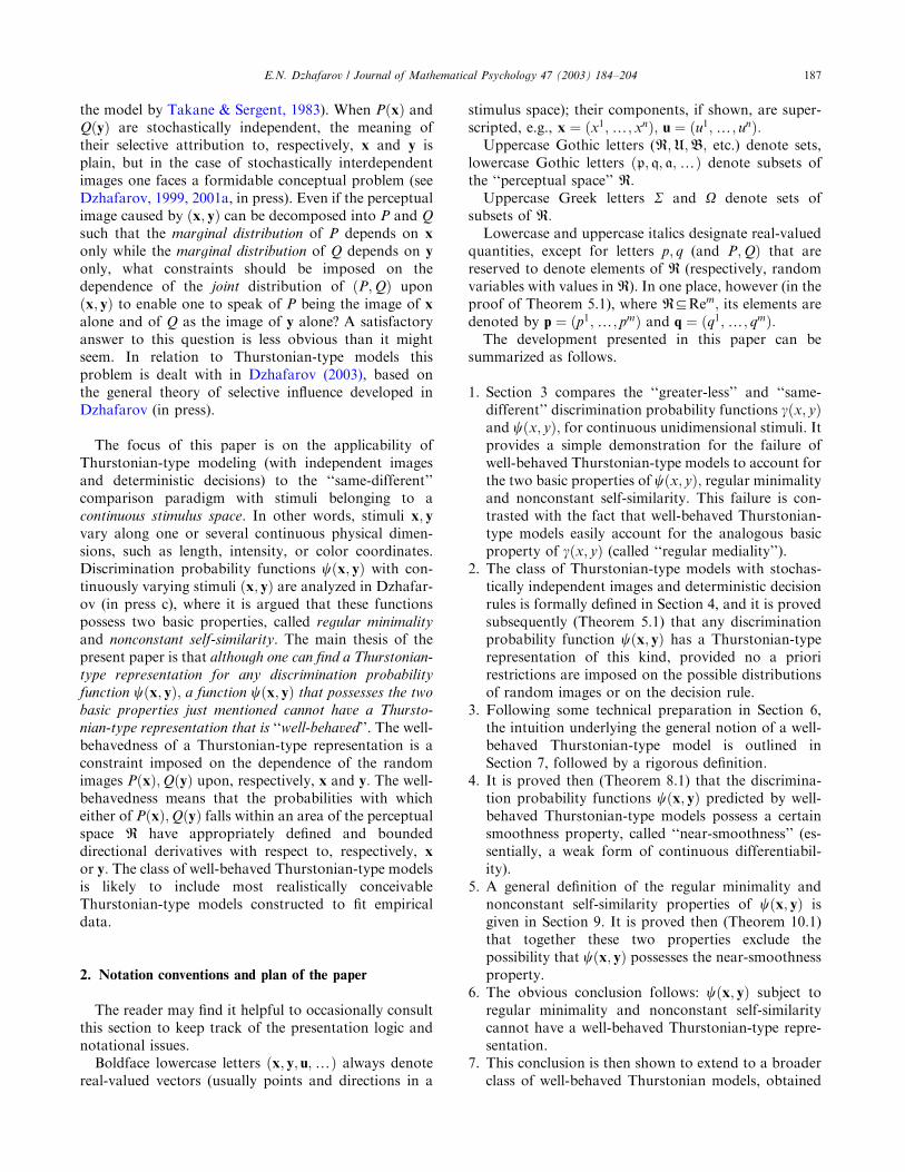
only, what constraints should be imposed on thedependence of the joint distribution of ðP;QÞ uponðx; yÞ to enable one to speak of P being the image of xalone and of Q as the image of y alone? A satisfactoryanswer to this question is less obvious than it mightseem. In relation to Thurstonian-type models thisproblem is dealt with in Dzhafarov (2003), based onthe general theory of selective influence developed inDzhafarov (in press).

The focus of this paper is on the applicability ofThurstonian-type modeling (with independent imagesand deterministic decisions) to the ‘‘same-different’’comparison paradigm with stimuli belonging to acontinuous stimulus space. In other words, stimuli x; yvary along one or several continuous physical dimen-sions, such as length, intensity, or color coordinates.Discrimination probability functions cðx; yÞ with con-tinuously varying stimuli ðx; yÞ are analyzed in Dzhafar-ov (in press c), where it is argued that these functionspossess two basic properties, called regular minimality

and nonconstant self-similarity. The main thesis of thepresent paper is that although one can find a Thurstonian-type representation for any discrimination probability

function cðx; yÞ; a function cðx; yÞ that possesses the twobasic properties just mentioned cannot have a Thursto-

nian-type representation that is ‘‘well-behaved’’. The well-behavedness of a Thurstonian-type representation is aconstraint imposed on the dependence of the randomimages PðxÞ;QðyÞ upon, respectively, x and y: The well-behavedness means that the probabilities with whicheither of PðxÞ;QðyÞ falls within an area of the perceptualspace R have appropriately defined and boundeddirectional derivatives with respect to, respectively, x

or y: The class of well-behaved Thurstonian-type modelsis likely to include most realistically conceivableThurstonian-type models constructed to fit empiricaldata.

2. Notation conventions and plan of the paper

The reader may find it helpful to occasionally consultthis section to keep track of the presentation logic andnotational issues.Boldface lowercase letters ðx; y; u;yÞ always denote

real-valued vectors (usually points and directions in a

stimulus space); their components, if shown, are super-scripted, e.g., x ¼ ðx1;y; xnÞ; u ¼ ðu1;y; unÞ:Uppercase Gothic letters (R;U;B; etc.) denote sets,

lowercase Gothic letters ðp; q; a;yÞ denote subsets ofthe ‘‘perceptual space’’ R:Uppercase Greek letters S and O denote sets of

subsets of R:Lowercase and uppercase italics designate real-valued

quantities, except for letters p; q (and P;QÞ that arereserved to denote elements of R (respectively, randomvariables with values inR). In one place, however (in theproof of Theorem 5.1), where RDRem; its elements aredenoted by p ¼ ðp1;y; pmÞ and q ¼ ðq1;y; qmÞ:The development presented in this paper can be

summarized as follows.

1. Section 3 compares the ‘‘greater-less’’ and ‘‘same-different’’ discrimination probability functions gðx; yÞand cðx; yÞ; for continuous unidimensional stimuli. Itprovides a simple demonstration for the failure ofwell-behaved Thurstonian-type models to account forthe two basic properties of cðx; yÞ; regular minimalityand nonconstant self-similarity. This failure is con-trasted with the fact that well-behaved Thurstonian-type models easily account for the analogous basicproperty of gðx; yÞ (called ‘‘regular mediality’’).

2. The class of Thurstonian-type models with stochas-tically independent images and deterministic decisionrules is formally defined in Section 4, and it is provedsubsequently (Theorem 5.1) that any discriminationprobability function cðx; yÞ has a Thurstonian-typerepresentation of this kind, provided no a priorirestrictions are imposed on the possible distributionsof random images or on the decision rule.

3. Following some technical preparation in Section 6,the intuition underlying the general notion of a well-behaved Thurstonian-type model is outlined inSection 7, followed by a rigorous definition.

4. It is proved then (Theorem 8.1) that the discrimina-tion probability functions cðx; yÞ predicted by well-behaved Thurstonian-type models possess a certainsmoothness property, called ‘‘near-smoothness’’ (es-sentially, a weak form of continuous differentiabil-ity).

5. A general definition of the regular minimality andnonconstant self-similarity properties of cðx; yÞ isgiven in Section 9. It is proved then (Theorem 10.1)that together these two properties exclude thepossibility that cðx; yÞ possesses the near-smoothnessproperty.

6. The obvious conclusion follows: cðx; yÞ subject toregular minimality and nonconstant self-similaritycannot have a well-behaved Thurstonian-type repre-sentation.

7. This conclusion is then shown to extend to a broaderclass of well-behaved Thurstonian models, obtained


by relaxing some of the constraints imposed inSection 7.

8. The development is aided by an appendix containinglemmas labeled A.1, A.2, etc.

To follow the mathematical derivations the readershould be familiar with basic concepts of abstractmeasure theory. With the help provided in the paper,however, knowledge of standard multivariate calculusshould be sufficient to understand the general logic andthe results.

3. Comparing two discrimination paradigms

To simplify the discussion, let the stimuli presentedfor a comparison judgment (‘‘greater-less’’, with respectto some attribute P; or ‘‘same-different’’) be physicallyunidimensional. In accordance with the general defini-tion of a continuous stimulus space given in the nextsection, the stimulus values x; y in this case belong to anopen interval of reals M (finite or infinite).As emphasized in Dzhafarov (2002d), the key fact

about pairwise presentations ðx; yÞ is that stimuli x andy belong to two distinct observation areas (spatial and/ortemporal intervals): thus, x may be presented first,followed by y; or x may be presented to the left and y tothe right of a fixation point. As a result, ðx; yÞ and ðy; xÞare distinct pairs, and ðx; xÞ is a pair of stimuli ratherthan a single stimulus. In the following the observationarea to which a stimulus belongs is encoded by itsordinal position within a pair ðx; yÞ; and the respectiveobservation areas are referred to as the ‘‘first’’ and the‘‘second’’ areas. One consequence of treating ðx; yÞ as anordered pair is that cðx; yÞ and cðy; xÞ in the ‘‘same-different’’ paradigm are generally different, and so aregðx; yÞ and 1� gðy; xÞ in the ‘‘greater-less’’ paradigm.(For a detailed discussion of distinct observation areassee Dzhafarov, 2002d)A central notion in the analysis of perceptual

discriminations is that of a point of subjective equality

(PSE). The intuitive meaning of this notion is as follows.For a given stimulus x (belonging to the first observa-tions area), a stimulus y (in the second observation area)is the PSE for x if the ‘‘subjective dissimilarity’’ betweenthis y and x is smaller than the dissimilarity between x

and any other stimulus belonging to the secondobservation area (generally, this point y need not beequal to x). Analogously, the PSE for y (belonging tothe second observation area) is the stimulus x (in thefirst observation area) whose dissimilarity to y is smallerthan that of any other stimulus taken in the firstobservation area. It seems natural to expect that areasonable operationalization of this notion shouldensure that a PSE for a given stimulus (in either

observation area) is uniquely defined, and that therelation of ‘‘being a PSE of’’ is symmetric:

y is the PSE for x 3 x is the PSE for y;

with x and y in both cases belonging to the first andsecond observation areas, respectively. Dzhafarov(2002d) proposes to treat this regularity property (theexistence, uniqueness, and symmetry of PSE) as afundamental law for perceptual discriminations.To discuss first the ‘‘greater-less’’ comparison para-

digm, refer to Figs. 1 and 3. In accordance with thetraditional psychophysical focus on ‘‘correlated’’ physi-cal and subjective continua, let the attributeP be chosenso that gðx; yÞ is strictly increasing in y and strictlydecreasing in x (recall that g is the probability that y; inthe second observation area, is judged to be greater thanx; in the first observation area). As an example, x; y mayrepresent physical intensity of successively presentedtones, and P their loudness. Let gðx; yÞ be continuous inðx; yÞ: Clearly, the PSE for x with respect to P should bedefined as the value of y for which gðx; yÞ ¼ 1

2; and the

same equality determines the PSE (with respect toP) fory: the value of x for which gðx; yÞ ¼ 1

2: Denoting the PSE

y

x

x1 x2 x3

y1 y2 y3

1/2

1/2

yγ

γ (x

, y)

x (

x, y

)

(x1, y) (x2, y) (x3, y)

γ γ γ

γ γ γ

(x, y1) (x, y2) (x, y3)

Fig. 3. Illustration of the regular mediality property. Shown are cross-

sections y-gðx; yÞ and x-gðx; yÞ of a ‘‘greater-less’’ discrimination

probability function gðx; yÞ for unidimensional continuous stimuli (seeFig. 1). The cross-sections y-gðx; yÞ shown in the upper panel are

made at arbitrarily chosen x ¼ x1;x2;x3: The cross-sections x-gðx; yÞshown in the lower panel are made at y ¼ y1; y2; y3 which are the

medians of the three curves in the upper panel. The regular mediality

property is illustrated by the fact that then x1; x2;x3 are the medians of

the three curves in the lower panel. In other words, yi is the median of

gðxi; yÞ if and only if xi is the median of gðx; yiÞ; i ¼ 1; 2; 3:


for x by hðxÞ; the PSE for y by gðyÞ; and assuming thatboth these functions are defined on the entire intervalM(i.e., a PSE exists for every stimulus, in either observa-tion area), a moment’s reflection reveals that both hðxÞand gðyÞ are one-to-one, onto, and continuous trans-formations M-M; and that g � h�1: By analogy withthe regular minimality property introduced below, thisfundamental regularity condition can be termed regular

mediality.Since regular mediality holds for any continuous

gðx; yÞ such that the equation gðx; yÞ ¼ 12can always be

solved for both x and y; this property is predicted by anyreasonable Thurstonian-type model, including Thursto-ne’s original theory. Let the perceptual space R be theset of reals, and let the random images PðxÞ;QðyÞ beindependent and normally distributed. Let their respec-tive means mPðxÞ; mQðyÞ be two arbitrarily smooth (e.g,infinitely differentiable) increasing functions M �!onto Reþ:Then one can always choose standard deviation func-tions sPðxÞ; sQðyÞ; also arbitrarily smooth, so that thediscrimination probability function

gðx; yÞ ¼ FmQðyÞ � mPðxÞffiffiffiffiffiffiffiffiffiffiffiffiffiffiffiffiffiffiffiffiffiffiffiffiffiffiffiffiffis2PðxÞ þ s2QðyÞ

q0B@

1CA;

where F is the standard normal integral, is increasing iny; decreasing in x; and continuous (in fact, arbitrarilysmooth) in ðx; yÞ: This is achieved, for example, if onechooses sPðxÞ � sP; sQðyÞ � sQ (constants), or sPðxÞ ¼kffiffiffiffiffiffiffiffiffiffiffiffimPðxÞ

p; sQðyÞ ¼ k

ffiffiffiffiffiffiffiffiffiffiffiffimQðyÞ

q; k40: Since mPðxÞ and

mQðyÞ have identical ranges ðReþÞ; the equationgðx; yÞ ¼ 1

2can be solved for y and x at, respectively,

any x and y; resulting in

hðxÞ ¼ m�1Q ½mPðxÞ�; gðyÞ ¼ m�1P ½mQðyÞ�:These functions satisfy the regular mediality conditionbecause g � h�1: Anticipating the subsequent develop-ment, the point to be emphasized here is that the regularmediality property for gðx; yÞ is predicted by Thursto-nian-type models that are arbitrarily ‘‘well-behaved’’(intuitively, PðxÞ;QðyÞ have ‘‘nice’’ distributions whoseparameters smoothly depend on stimuli).The situation changes dramatically as we turn to

‘‘same-different’’ comparisons. Refer to Figs. 2 and 4. Inaccordance with the so-called ‘‘First Assumption ofmultidimensional Fechnerian scaling’’ (discussed ingreater generality in Section 9), cðx; yÞ is continuousin ðx; yÞ; y-cðx; yÞ reaches a global minimum at somepoint hðxÞ; continuously changing with x; andx-cðx; yÞ reaches a global minimum at some pointgðyÞ; continuously changing with y: Clearly, hðxÞ shouldbe taken as the PSE for x; and gðyÞ as the PSE for y: Thesymmetry of the PSE relation in this case, g � h�1; iscalled the property of regular minimality. Unlike theregular mediality above, this property is not a mathe-

matical necessity, but it is both intuitively plausible andcorroborated by available empirical evidence (seeDzhafarov, 2002d). It is also known (Dzhafarov,2002d) that the minimum level cðx; hðxÞÞ of the functiony-cðx; yÞ is generally different for different values of x;and, analogously, the minimum level cðgðyÞ; yÞ of thefunction x-cðx; yÞ is generally different for differentvalues of y: This well-documented property is callednonconstant self-similarity. It has no analogue in the‘‘greater-less’’ discrimination probability functions,where the level of gðx; yÞ at which the PSE are taken is12by definition.

Remark 3.1. The term ‘‘self-similarity’’ (or ‘‘self-dissim-ilarity’’) is due to the fact that ‘‘ideally’’ the minima ofthe functions y-cðx; yÞ and x-cðx; yÞ are reached at

y

x

x1 x2 x3

y1 y2 y3

yψ

ψ

(x

, y)

x (

x, y

)

(x1, y) (x2, y)

(x3, y)

(x, y1)ψ

ψ

ψ

ψ

ψ

ψ

(x, y2)

(x, y3)

Fig. 4. Illustration of the regular minimality and nonconstant self-

similarity properties. Shown are cross-sections y-cðx; yÞ and

x-cðx; yÞ of a ‘‘same-different’’ discrimination probability function

cðx; yÞ for unidimensional continuous stimuli (see Fig. 2). The cross-sections y-cðx; yÞ shown in the upper panel are made at arbitrarily

chosen x ¼ x1;x2; x3: The cross-sections x-cðx; yÞ shown in the lowerpanel are made at y ¼ y1; y2; y3 which are the points at which the three

curves in the upper panel reach their minima. The regular minimality

property is illustrated by the fact that then x1;x2;x3 are the points at

which the three curves in the lower panel reach their minima. In other

words, arg minycðxi; yÞ ¼ yi if and only if arg minxcðx; yiÞ ¼ xi; i ¼1; 2; 3: The nonconstant self-similarity property is illustrated by the

fact that the minimum level cðxi ; yiÞ is different for different PSE pairs

ðxi ; yiÞ; i ¼ 1; 2; 3:


y ¼ x; in which case it is said that there is no constant

error.

Can these two properties, regular minimality andnonconstant self-similarity, be predicted by a Thursto-nian-type model with ‘‘nicely’’ distributed and ‘‘nicely’’dependent on stimuli images, like the ones usedabove to model gðx; yÞ? It turns out that any attemptto come up with such a model will fail. Take, forexample, the same PðxÞ;QðyÞ as used above, indepen-dent and normally distributed on the set of reals,with their means mPðxÞ; mQðyÞ being smooth increasing

functions M �!onto Reþ and their standard deviations

being chosen as either sPðxÞ � sP; sQðyÞ � sQ (con-

stants) or sPðxÞ ¼ kffiffiffiffiffiffiffiffiffiffiffiffimPðxÞ

p; sQðxÞ ¼ k

ffiffiffiffiffiffiffiffiffiffiffiffimQðxÞ

q: Let

the decision rule be the symmetric version of theone proposed by Luce and Galanter (1963): ‘‘say thaty is different from x if and only if jPðxÞ �QðyÞj4e’’.Then

cðx; yÞ ¼ 1� Fe� ½mQðyÞ � mPðxÞ�ffiffiffiffiffiffiffiffiffiffiffiffiffiffiffiffiffiffiffiffiffiffiffiffiffiffiffiffiffi

s2PðxÞ þ s2QðyÞq

0B@

1CA

þ F�e� ½mQðyÞ � mPðxÞ�ffiffiffiffiffiffiffiffiffiffiffiffiffiffiffiffiffiffiffiffiffiffiffiffiffiffiffiffiffi

s2PðxÞ þ s2QðyÞq

0B@

1CA:

Choosing first sPðxÞ � sP; sQðyÞ � sQ; one can easilyshow that y-cðx; yÞ and x-cðx; yÞ reach their minimaat, respectively,

y ¼ m�1Q ½mPðxÞ� ¼ hðxÞ; x ¼ m�1P ½mQðyÞ� ¼ gðyÞ;

which are the same functions as obtained above for

gðx; yÞ; satisfying thereby the requirement g � h�1: Withconstant standard deviations, however, the minimumlevel of y-cðx; yÞ and x-cðx; yÞ is constant,

cðx; hðxÞÞ ¼ cðgðyÞ; yÞ ¼ 2F�effiffiffiffiffiffiffiffiffiffiffiffiffiffiffiffiffi

s2P þ s2Qq

0B@

1CA:

The cðx; yÞ generated by this model, therefore, whilesatisfying the regular minimality condition, also has theproperty of constant self-similarity.Choosing sPðxÞ ¼ k

ffiffiffiffiffiffiffiffiffiffiffiffimPðxÞ

p; sQðxÞ ¼ k

ffiffiffiffiffiffiffiffiffiffiffiffimQðxÞ

qdoes

make the minimum levels of y-cðx; yÞ and x-cðx; yÞvary with, respectively, x and y; satisfying thereby thenonconstant self-similarity requirement. By a simplethough cumbersome derivation, however, one can showthat in this case one loses the regular minimalityproperty: in fact, one cannot find a single pair ðx; yÞ atwhich the functions y-cðx; yÞ and x-cðx; yÞ reach

their minima simultaneously. Indeed, denoting

Aðx; y; eÞ ¼ exp �ðeþ mQðyÞ � mPðxÞÞ22k2ðmQðyÞ þ mPðxÞÞ

" #;

Bðx; y; eÞ ¼ exp �ðe� mQðyÞ þ mPðxÞÞ22k2ðmQðyÞ þ mPðxÞÞ

" #;

the conditions @cðx;yÞ@y ¼ 0 and @cðx;yÞ

@x ¼ 0 can be shown tobe equivalent to, respectively,

½mQðyÞ þ 3mPðxÞ � e�Aðx; y; eÞ� ½mQðyÞ þ 3mPðxÞ þ e�Bðx; y; eÞ ¼ 0

and

½3mQðyÞ þ mPðxÞ þ e�Aðx; y; eÞ� ½3mQðyÞ þ mPðxÞ � e�Bðx; y; eÞ ¼ 0:

Their addition yields

½mQðyÞ þ mPðxÞ�½Aðx; y; eÞ � Bðx; y; eÞ� ¼ 0;

which can easily be proved impossible for positive mPðxÞ;mQðyÞ; and e:The subsequent development shows that these Thur-

stonian-type models cannot be repaired by any mod-ifications of the perceptual space R; decision rules, ordistributions of PðxÞ and QðyÞ; insofar as the depen-dence of these distributions on stimuli x; y remainssufficiently ‘‘well-behaved’’. For the ‘‘same-different’’discrimination probabilities cðx; yÞ the conjunction ofthe properties of regular minimality and nonconstantself-similarity is incompatible with well-behaved Thur-stonian-type representations. In a sense, the only reasonsuch representations are possible for the ‘‘greater-less’’discrimination probabilities gðx; yÞ is that there is noanalog of nonconstant self-similarity for these functions:by definition, the regular mediality property is asso-ciated with the fixed probability level 1

2:

A rigorous and general definition for the notion of‘‘well-behavedness’’ is given in Section 7 (furthergeneralized in Section 11). Put semi-formally, in thecase of unidimensional continuous stimuli the ‘‘well-behavedness’’ of, say, the distribution of PðxÞ at a pointx ¼ x0 means that in a sufficiently small neighborhood½x0 � a; x0 þ a� the probabilities Pr½PðxÞAp� for allpossible events p have bounded right- and left-handderivatives with respect to x:

4. Thurstonian-type representations

A Thurstonian-type representation (with independentrandom images and a deterministic decision rule) for adiscrimination probability function cðx; yÞ is defined by


the construct

fR;Ax;By;Sg; ð1Þwith the following meaning of the terms.

(i) x and y are stimuli whose values belong to an n-dimensional continuous stimulus space

MDRen ðnX1Þ; an open connected area with itsdimensions representing physical attributes varyingin the experiment. As discussed in the previoussection, x and y belong to distinct observation areas(spatial and/or temporal intervals), encoded by theirpositions within the pair ðx; yÞ: The representationM for a given set of physical stimuli is not unique:any homeomorphic (one-to-one, onto, continuoustogether with its inverse) mapping M-M0DRen

creates an equivalent representation for the stimulusspace. This means, in particular, that Ren in theinclusion MDRen can always be replaced by anysubset of Ren homeomorphically related to Ren

(e.g., an open n-dimensional unit cube).

Remark 4.1. It is allowed, if convenient, to applydifferent homeomorphic transformations to stimuliin the first and second observation areas, includingthe possibility that they map onto different sets,M0;M00:It may have been better, therefore, to speak oftwo generally different stimulus spaces for x and for y

in ðx; yÞ: The notion of a single stimulus space isretained in the present paper for expository simplicityonly.

(ii) R is a hypothetical perceptual space, whose pointsp; q;y are referred to as (perceptual) images. Norestrictions are imposed on its possible structure: itcan be a finite set of states, an area of Rem; a spaceof continuous processes, a space of compact areasbelonging to Rem; etc. The term ‘‘space’’ (ratherthan ‘‘set’’) is used here due to the structureimposed on R by the probability measures con-sidered next.

(iii) AxðpÞ and ByðqÞ; p; qDR; are probability measures

defined on respective sigma-algebras SA; SB; thesame for all values of x; y: (A sigma-algebra is a setof subsets of R that includes R and is closed undercountable applications of standard set-theoreticoperations.) AxðpÞ and ByðqÞ are associated withrandom images PðxÞ and QðyÞ of stimuli x and y;

AxðpÞ ¼ Pr½PðxÞAp�; pASA;

ByðqÞ ¼ Pr½QðyÞAq�; qASB:

The measures Ax and By; as well as their domainsSA and SB; are generally different, to reflect thefact that x and y belong to distinct observationareas.

Remark 4.2. In the simplest case, when R is a finite setof states f1;y; kg; the distributions of PðxÞ and QðyÞare defined by aði; xÞ ¼ Pr½PðxÞ ¼ i� and bði; yÞ ¼Pr½QðyÞ ¼ i�; i ¼ 1;y; k: In this case, AxðpÞ ¼P

iAp aði; xÞ; ByðqÞ ¼P

iAq bði; yÞ; and SA ¼ SB is theset of all 2k subsets of f1;y; kg: The reader who wishesto overlook measure-theoretic technicalities may thinkof this example throughout the paper, ignoring allreferences to sigma-algebras and measurability.

(iv) SDR�R is the area that determines (and isdetermined by) a decision rule: x and y are judgedto be different in a given trial if and only ifðp; qÞAS; where p and q are the values of,respectively, PðxÞ and QðyÞ in this trial. For brevity,I refer to S as the decision area, instead of the moreexplicit ‘‘area corresponding to the decision that xand y are different’’. (Nothing would have changedin the treatment to follow if we considered insteadthe complementary area, mapped into the response‘‘same’’.) The measures Ax and By induce on R�Rthe probabilistic product measure ABxy ¼ Ax � By;defined on the sigma-algebra SAB generated bySA � SB;

ABxyðsÞ ¼ Pr½ðPðxÞ;QðyÞÞAs�; sASAB:

The decision area S is assumed to be AB-measur-able (i.e., ASAB).

Remark 4.3. One can say ‘‘AB-measurable’’ ratherthan ‘‘ABxy-measurable’’ because the sigma-algebraSAB is the same for all ðx; yÞ: Analogously, theterms ‘‘A -measurable’’ and ‘‘B-measurable’’ are usedbelow instead of ‘‘Ax-measurable’’ and ‘‘By-measur-able’’.

Remark 4.4. For R ¼ f1;y; kg introduced in Remark4.2, SAB is the set of all 2

k2 subsets of the set f1;y; kg �f1;y; kg; and ABxyðsÞ ¼

Pði;jÞAs aði; xÞbð j; yÞ:

(v) The general relation between the unobservablesfR;Ax;By;Sg of the model and the observablecðx; yÞ is given by

cðx; yÞ ¼ Pr½ðPðxÞ;QðyÞÞAS� ¼ ABxyðSÞ:We have (see, e.g., Hewitt & Stromberg, 1965, p.384)

ABxyðSÞ ¼ZqAR

Ax½aðqÞ� dByðqÞ

¼ZpAR

By½bð pÞ� dAxð pÞ; ð2Þ


where

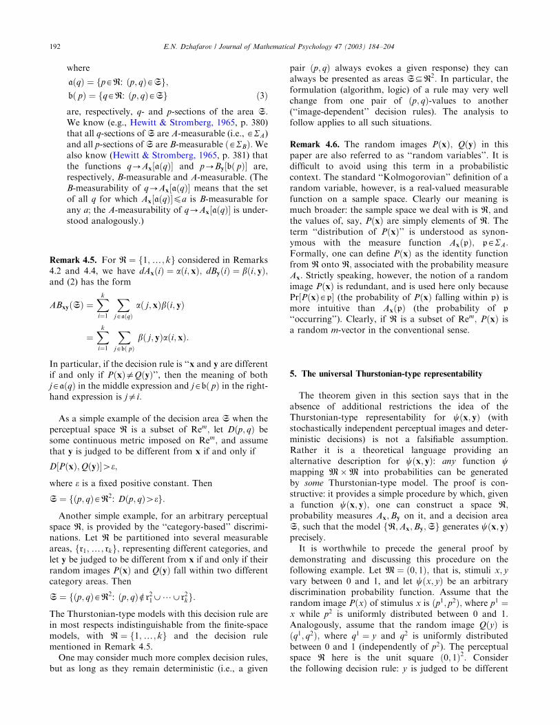
aðqÞ ¼ fpAR: ðp; qÞASg;bð pÞ ¼ fqAR: ðp; qÞASg ð3Þare, respectively, q- and p-sections of the area S:We know (e.g., Hewitt & Stromberg, 1965, p. 380)that all q-sections of S are A-measurable (i.e., ASA)and all p-sections ofS are B-measurable ðASBÞ:Wealso know (Hewitt & Stromberg, 1965, p. 381) thatthe functions q-Ax½aðqÞ� and p-By½bð pÞ� are,respectively, B-measurable and A-measurable. (TheB-measurability of q-Ax½aðqÞ� means that the setof all q for which Ax½aðqÞ�pa is B-measurable forany a; the A-measurability of q-Ax½aðqÞ� is under-stood analogously.)

Remark 4.5. For R ¼ f1;y; kg considered in Remarks4.2 and 4.4, we have dAxðiÞ ¼ aði; xÞ; dByðiÞ ¼ bði; yÞ;and (2) has the form

ABxyðSÞ ¼Xki¼1

XjAaðqÞ

að j; xÞbði; yÞ

¼Xki¼1

XjAbð pÞ

bð j; yÞaði; xÞ:

In particular, if the decision rule is ‘‘x and y are differentif and only if PðxÞaQðyÞ’’, then the meaning of bothjAaðqÞ in the middle expression and jAbð pÞ in the right-hand expression is jai:

As a simple example of the decision area S when theperceptual space R is a subset of Rem; let Dðp; qÞ besome continuous metric imposed on Rem; and assumethat y is judged to be different from x if and only if

D½PðxÞ;QðyÞ�4e;

where e is a fixed positive constant. Then

S ¼ fðp; qÞAR2: Dðp; qÞ4eg:Another simple example, for an arbitrary perceptual

space R; is provided by the ‘‘category-based’’ discrimi-nations. Let R be partitioned into several measurableareas, fr1;y; rkg; representing different categories, andlet y be judged to be different from x if and only if theirrandom images PðxÞ and QðyÞ fall within two differentcategory areas. Then

S ¼ fðp; qÞAR2: ðp; qÞer21,?,r2kg:The Thurstonian-type models with this decision rule arein most respects indistinguishable from the finite-spacemodels, with R ¼ f1;y; kg and the decision rulementioned in Remark 4.5.One may consider much more complex decision rules,

but as long as they remain deterministic (i.e., a given

pair ðp; qÞ always evokes a given response) they canalways be presented as areas SDR2: In particular, theformulation (algorithm, logic) of a rule may very wellchange from one pair of ðp; qÞ-values to another(‘‘image-dependent’’ decision rules). The analysis tofollow applies to all such situations.

Remark 4.6. The random images PðxÞ; QðyÞ in thispaper are also referred to as ‘‘random variables’’. It isdifficult to avoid using this term in a probabilisticcontext. The standard ‘‘Kolmogorovian’’ definition of arandom variable, however, is a real-valued measurablefunction on a sample space. Clearly our meaning ismuch broader: the sample space we deal with is R; andthe values of, say, PðxÞ are simply elements of R: Theterm ‘‘distribution of PðxÞ’’ is understood as synon-ymous with the measure function AxðpÞ; pASA:Formally, one can define PðxÞ as the identity functionfrom R onto R; associated with the probability measureAx: Strictly speaking, however, the notion of a randomimage PðxÞ is redundant, and is used here only becausePr½PðxÞAp� (the probability of PðxÞ falling within p) ismore intuitive than AxðpÞ (the probability of p‘‘occurring’’). Clearly, if R is a subset of Rem; PðxÞ isa random m-vector in the conventional sense.

5. The universal Thurstonian-type representability

The theorem given in this section says that in theabsence of additional restrictions the idea of theThurstonian-type representability for cðx; yÞ (withstochastically independent perceptual images and deter-ministic decisions) is not a falsifiable assumption.Rather it is a theoretical language providing analternative description for cðx; yÞ: any function cmapping M�M into probabilities can be generatedby some Thurstonian-type model. The proof is con-structive: it provides a simple procedure by which, givena function cðx; yÞ; one can construct a space R;probability measures Ax;By on it, and a decision areaS; such that the model fR;Ax;By;Sg generates cðx; yÞprecisely.It is worthwhile to precede the general proof by

demonstrating and discussing this procedure on thefollowing example. Let M ¼ ð0; 1Þ; that is, stimuli x; yvary between 0 and 1, and let cðx; yÞ be an arbitrarydiscrimination probability function. Assume that therandom image PðxÞ of stimulus x is ðp1; p2Þ; where p1 ¼x while p2 is uniformly distributed between 0 and 1.Analogously, assume that the random image QðyÞ isðq1; q2Þ; where q1 ¼ y and q2 is uniformly distributedbetween 0 and 1 (independently of p2). The perceptualspace R here is the unit square ð0; 1Þ2: Considerthe following decision rule: y is judged to be different


from x if and only if

0op2offiffiffiffiffiffiffiffiffiffiffiffiffiffiffiffiffifficðp1; q1Þ

qand 0oq2o

ffiffiffiffiffiffiffiffiffiffiffiffiffiffiffiffiffifficðp1; q1Þ

q: ð4Þ

A moment’s contemplation will reveal that the prob-ability of this happening is cðx; yÞ:Some readers may feel uncomfortable about the fact

that the first component of the image PðxÞ ¼ ðp1; p2Þ inthis construction is a deterministic quantity ðp1 ¼ xÞ:Clearly, the perceiver could achieve perfect discrimin-ability by simply ignoring the second component ofPðxÞ: It would be a mistake, however, to dismiss themodel above on the grounds that its decision rule is‘‘irrational’’ or ‘‘suboptimal’’. We expressly lack anybasis for applying these concepts, as they only makesense with respect to a particular set of operations thatthe perceiver is posited to have the option of applying tothe elements of R: Thus, it does not follow from the factthat ðp1; p2Þ uniquely determines the value of expðp1Þ þexpðp2Þ that the perceiver is able to use this number formaking a judgment. By the same logic, it does not followfrom the fact that a perceptual image can be representedby a numerical vector that the perceiver is able to usethis vector’s components in all conceivable computa-tions or judgments involving them. In general, given aThurstonian-type representation, the only operationthat the perceiver can and should be posited to performis the computation, for every pair of images ðp; qÞ; ofwhether this pair belongs or does not belong to onespecific decision area S: In the construction above, forexample, the observer is assumed to compute the truthvalue of the statement (4), but this does not imply thatthis observer can extract and utilize p2; q2; or cðp1; q1Þ inany other computation.Note that one can easily modify this construction to

make both components of the random images stochas-tic. Assume, for example, that PðxÞ ¼ ðp1; p2Þ andQðyÞ ¼ ðq1; q2Þ are defined by

p1 ¼ v� x

2; p2 ¼ vþ x

2;

q1 ¼ w� y

2; q2 ¼ wþ y

2;

where v;w are independent random variables uniformlydistributed between 0 and 1. Modify the decision ruleaccordingly: y is judged to be different from x if andonly if

0op1 þ p2offiffiffiffiffiffiffiffiffiffiffiffiffiffiffiffiffiffiffiffiffiffiffiffiffiffiffiffiffiffiffiffiffiffiffiffiffifficðp2 � p1; q2 � q1Þ

q;

0oq1 þ q2offiffiffiffiffiffiffiffiffiffiffiffiffiffiffiffiffiffiffiffiffiffiffiffiffiffiffiffiffiffiffiffiffiffiffiffiffifficðp2 � p1; q2 � q1Þ

q:

It is easy to see that this model is equivalent to theprevious one, because of which it too generates cðx; yÞprecisely.

Theorem 5.1. Any function c : ðx; yÞ-½0; 1� has a

Thurstonian-type representation fR;Ax;By;Sg (with

stochastically independent images and a deterministic

decision rule).

Proof. With no loss of generality, let x; yAMDð0; 1Þn(this can always be achieved by a suitable home-omorphic transformation of M). Define the perceptualspace R as

R ¼ M� ð0; 1ÞDð0; 1Þnþ1;

with the conventional Lebesgue sigma-algebra S on it.Denote the elements of R by p ¼ ðp0; pnþ1Þ; with p0 ¼ðp1;y; pnÞ: Note that p0 may or may not belong to theset MDð0; 1Þn:For any p0AM; q0AM; define sðp0; q0Þ as the square

region

sðp0; q0Þ ¼ ð0;ffiffiffiffiffiffiffiffiffiffiffiffiffiffiffiffifficðp0; q0Þ

pÞ � ð0;

ffiffiffiffiffiffiffiffiffiffiffiffiffiffiffiffifficðp0; q0Þ

pÞ;

and choose the decision area SDR2Dð0; 1Þ2nþ2 to be

S ¼ fðp; qÞ: p0AM; q0AM; ðpnþ1; qnþ1ÞAsðp0; q0Þg:

(In this construction sðp0; q0Þ could be replaced with anyother subset of ð0; 1Þ2 whose Lebesgue measure iscðp0; q0Þ:)Put SA ¼ SB ¼ S; the set of all Lebesgue-measurable

subsets. For rAS; define

AxðrÞ ¼ZpAr

aðp; xÞ dp; ByðrÞ ¼ZqAr

aðq; yÞ dq;

with the (generalized) density functions a and b definedas

aðp; xÞ ¼ dðp0 � xÞ; bðq; yÞ ¼ dðq0 � yÞ;

where d is the (multivariate) Dirac delta function. AxðrÞis a legitimate probability measure on S; becauseaðp; xÞX0; and

ZpAR

aðp; xÞ dp

¼Zp0AM

Z 1

0

dðp0 � xÞ dpnþ1 dp0

¼Zp0AM

dðp0 � xÞZ 1

0

dpnþ1� �

dp0 ¼ 1;


analogously for ByðrÞ: ThenABxyðSÞ

¼Zðp;qÞAS

aðp; xÞbðq; yÞ dp dq

¼Zp0AM

Zq0AM

Zðpnþ1;qnþ1ÞAsðp0;q0Þ

dðp0 � xÞ

� dðq0 � yÞ dqnþ1 dpnþ1 dq0 dp0

¼Zp0AM

Zq0AM

dðp0 � xÞdðq0 � yÞ

�Zðpnþ1;qnþ1ÞAsðp0;q0Þ

dqnþ1 dpnþ1 !

dq0 dp0

¼Zp0AM

Zq0AM

dðp0 � xÞdðq0 � yÞcðp0; q0Þ dq0 dp0

¼ cðx; yÞ:This completes the construction of a Thurstonian-typerepresentation for cðx; yÞ: &

Remark 5.1. To generalize the concluding part of thediscussion that precedes the theorem, once a Thursto-nian-type representation for cðx; yÞ is constructed, onecan construct another representation by (a) replacing Rwith R� ¼ FðRÞ; where F is any one-to-one transforma-tion, (b) defining the sigma-algebra S� on R� by the rule‘‘rAS� if and only if F�1ðrÞAS’’ (which makes F ameasurable mapping), (c) putting A�

xðrÞ ¼ Ax½F�1ðrÞ�;B�yðrÞ ¼ By½F�1ðrÞ�; and (d) defining S�DR� �R� by

the rule ‘‘ðp; qÞAS� if and only if ðF�1ð pÞ;F�1ðqÞÞAS’’.Then, obviously, A�B�

xyðS�Þ ¼ ABxyðSÞ ¼ cðx; yÞ:

It must be emphasized that the sole purpose of thistheorem is to show that some Thurstonian-type repre-sentation exists for every imaginable discriminationprobability function. It is hardly worth mentioning thatthe construction described in the theorem (or any of itsmodifications mentioned in Remark 5.1) is of no interestto a model-builder: the probability measures Ax and By

used in the proof are singular, concentrated on sets ofmeasure zero, and the decision rule is void of anyinterpretability. An adherent of the idea that stimuli aremapped into random variables is likely to think of moreregular, ‘‘better behaved’’ random variables, like multi-variate or univariate normal distributions, combinedwith some easily interpretable decision rule, such as thedistance-based or category-based rules mentioned at theend of Section 4 (Dai, Versfeld, & Green, 1996; Ennis,1992; Ennis et al., 1988; Luce & Galanter, 1963; Sorkin,1962; Suppes & Zinnes, 1963; Thomas, 1996, 1999;Zinnes & MacKey, 1983).Unfortunately for this line of modeling, it is doomed

to fail. As shown in this paper, even if decision rules arenot constrained to be reasonable or interpretable, norealistic discrimination probability function can be

accounted for by sufficiently ‘‘nice’’ distributions withparameters sufficiently ‘‘nicely’’ dependent on stimuli.

Remark 5.2. In relation to the notion of well-behavedThurstonian-type representations (to be defined inSection 7), it is useful to observe just in what respectthe distribution constructed in Theorem 5.1 fails to be‘‘nice’’. For every random variable in R one can choosea measurable subset r of R and ask with whatprobability AxðrÞ the random variable falls in thissubset. With R and AxðrÞ defined as in Theorem 5.1,choose

r0 ¼ fp ¼ ðp0; pnþ1Þ: p0 ¼ ðp10;y; pn0Þ; pnþ1Að0; 1Þg:Then Axðr0Þ ¼ 0 for any xaðp10;y; pn0Þ; but the value ofAxðrÞ ‘‘jumps’’ to 1 as soon as x ¼ ðp10;y; pn0Þ: Thisviolates the main intuition behind the notion of well-behavedness, which is that for any r the value of AxðrÞmust change with x continuously.

6. Patches of discrimination probabilities

Here, I introduce a local parametrization of stimulithat greatly simplifies the development by replacing inall subsequent arguments the n-component stimuli x ¼ðx1;y; xnÞ; y ¼ ðy1;y; ynÞ with certain unidimensionalrepresentations thereof, denoted x; y:This local parametrization is achieved by choosing a

particular stimulus sAMDRen; a nonzero direction ofchange uARen (a stimulus–direction combination ðs; uÞis traditionally called a line element), and consideringvalues of x varying within an arbitrarily small vicinity ofs along the direction u;

x ¼ sþ ux; xA½�a; a�; a40:

Recall that M is open, because of which one can alwaysfind a sufficiently small a (generally depending on s; u)such that x ¼ sþ ux belongs to M for all xA½�a; a�:Clearly, for a fixed line element ðs; uÞ the value of x isuniquely encoded by x: Since we are interested in anarbitrarily small vicinity of s; the precise value of a isnever the issue: it can be made as small as one wishes.Let now h be a fixed homeomorphism M-M: Then,

for any yA½�a; a�; the value y ¼ hðsþ uyÞ is uniquelyencoded by y: As y varies within ½�a; a�; the values of yform a segment of a continuous curve lying within M:The set

fðx; yÞ: x ¼ sþ ux; y ¼ hðsþ uyÞ; ðx; yÞA½�a; a�2gthen belongs to M2; that is, consists of stimulus pairs.Once the line element ðs; uÞ and the homeomorphism h

are fixed, all stimulus pairs within this set are uniquelyparametrized by ðx; yÞA½�a; a�2: In particular, any twocorresponding stimuli x and y ¼ hðxÞ are encoded by


equal local coordinates �apx ¼ ypa; and the ‘‘cen-tral’’ pair ðs; hðsÞÞ is represented by x ¼ y ¼ 0:

Remark 6.1. Anticipating the material of Section 9(although sufficiently prompted by the discussion inSection 3), the homeomorphism h that we are interestedin is the one that relates x to its PSE y ¼ hðxÞ: At suchpairs of stimuli the functions x-cðx; yÞ and y-cðx; yÞreach their minima,

hðxÞ ¼ arg miny

cðx; yÞ; h�1ðyÞ ¼ arg minx

cðx; yÞ:

The local parametrization being constructed, therefore,focuses one’s attention on the stimulus values varying inarbitrarily small vicinities of the minima of cðx; yÞ: Fornow, however (until Section 10), this interpretation of his not essential, and h can be taken as an arbitrary fixedhomeomorphism.

The function

cðs;uÞðx; yÞ ¼ cðsþ ux; hðsþ uyÞÞ ð5Þdefined on ðx; yÞA½�a; a�2 is called a patch of thediscrimination probability function cðx; yÞ at the lineelement ðs; uÞ: For a fixed ðs; uÞ; it is convenient to dropthe index in (5) and to simply speak of a patch cðx; yÞ;omitting or mentioning ðs; uÞ and the patch domain½�a; a�2 as needed. The homeomorphism h is assumed tobe fixed throughout and need not be mentioned at all.For any patch cðx; yÞ of cðx; yÞ taken at some line

element ðs; uÞ; one can rewrite Ax; By; ABxy as Axð pÞ;ByðqÞ; ABxy; to present the basic relationship (2) as

cðx; yÞ ¼ ABxyðSÞ ¼ZqAR

Ax½aðqÞ� dByðqÞ

¼ZpAR

By½bð pÞ� dAxð pÞ; ð6Þ

where ðp; qÞAR2; ðx; yÞA½�a; a�2: Recall, from Section 4,that the functions q-Ax½aðqÞ� and p-By½bð pÞ� are,respectively, B-measurable and A-measurable.It is important to observe that representation (2) may

fail to hold for cðx; yÞ even if (6) holds for all possiblepatches cðx; yÞ: For one thing, the stimulus spaceM andthe homeomorphism h may very well be such that somestimulus pairs ðx; yÞ will not be covered by any of thepatches. Also, it is possible that the perceptual space R;probability measures Axð pÞ; ByðqÞ; and a decision areaS satisfying (6) can be found for any patch cðx; yÞ;taken separately, but cannot be combined into a singleThurstonian-type representation across all the patches(this will happen whenever, say, Axð pÞ is different on thecommon part of two overlapping patches). This is thereason why Theorem 5.1, asserting the existence of aThurstonian-type representation, has to be proved forthe entire discrimination probability function cðx; yÞrather than for its arbitrary patch cðx; yÞ:

At the same time, representation (2) holds only if (6)holds for all possible patches cðx; yÞ of cðx; yÞ:Equivalently put, if (6) does not hold for a single patchcðx; yÞ; then (2) does not hold for cðx; yÞ: Therefore toprove that cðx; yÞ subject to the regular minimality andnonconstant self-similarity constraints (discussed inSection 3 and defined in Section 9) cannot have a‘‘well-behaved’’ Thurstonian-type representation (de-fined in the next section), it is sufficient to show thatthere is at least one patch cðx; yÞ of this cðx; yÞ thatdoes not have a ‘‘well-behaved’’ Thurstonian-typerepresentation. In fact, the development to follow showsthis to be true for any ‘‘typical’’ patch cðx; yÞ (as definedin Section 9).

7. Well-behavedness

Having fixed a line element ðs; uÞ; consider aprobabilistic measure

AxðpÞ ¼ Pr½PðxÞAp�;

with x varying, in accordance with the ‘‘patch-wise’’view just introduced, within an interval ½�a; a� that canbe made arbitrarily small.A natural intuition for the ‘‘well-behavedness’’ of

AxðpÞ is that, for any fixed event ð¼ measurable setÞ p;its probability AxðpÞ must change ‘‘sufficientlysmoothly’’ in response to transitions x-xþ dx withina very small ½�a; a�: In the definition below this intuitionis translated into the existence of unilateral derivatives@

@xþAxðpÞ and @@x�AxðpÞ: In practice, we almost always

translate the idea of ‘‘sufficient smoothness’’ intopiecewise continuous differentiability (i.e., continuousdifferentiability with a countable number of isolatedexceptions). Thus, a freehand drawing of a continuouscurve, however ‘‘jittery’’, is always parametricallyrepresentable by a pair of piecewise continuouslydifferentiable functions. It seems that all continuousfunctions of applied mathematics are piecewise con-tinuously differentiable. The requirement of unilateraldifferentiability adopted in this paper is even lessstringent. In accordance with Lemma A.1, for anygiven p; the set of points xA½�a; a� where @

@xþAxðpÞa@

@x�AxðpÞ is at most denumerable (i.e., empty, finite, orcountably infinite), but it need not be a set of isolatedpoints. Outside this countable set, AxðpÞ is differentiableon ½�a; a� in the conventional sense, but its derivative isnot required to be continuous.The unilateral differentiability of AxðpÞ prevents the

latter from ‘‘jumping’’ in response to x-xþ dx: One’sintuition of well-behavedness, however, requires, inaddition, that AxðpÞ may not come arbitrarily close to‘‘jumping’’: AxðpÞ is not well-behaved if, for any


½�a; a�; however small,AxðpÞ � Ax0 ðpÞ

x� x0

��

can be made arbitrarily large by an appropriate choiceof p and of two distinct x; x0 within ½�a; a�: This meansthat a well-behaved AxðpÞ should satisfy the Lipschitz

condition:

Ax0 ðpÞ � AxðpÞx0 � x

��oconst

for some choice of a and all x; x0A½�a; a�; pASA: By astandard calculus argument, if AxðpÞ is unilaterallydifferentiable, the Lipschitz condition is equivalent tothe boundedness of the unilateral derivatives:

@

@x7AxðpÞ

��oconst

for all xA½�a; a� and pASA:It is important to note that, by Lemma A.2, the

Lipschitz condition implies that the unilateral deriva-tives @

@x7AxðpÞ exist (and are then necessarily bounded)at all points of ½�a; a�; except, perhaps, on a set ofmeasure zero. The intuition of ‘‘sufficient smoothness’’therefore can also be presented as an additionalregularization of the Lipschitz condition, the require-ment that the exceptional sets of measure zero be emptyfor all pASA:

Definition 7.1. A probabilistic measure AxðpÞ; pASA;xA½�a; a�; is well-behaved if the left- and right-handderivatives

D7A ðp; xÞ ¼ @AxðpÞ

@x7

exist and are bounded on SA � ½�a; a�; that is,jD7

A ðp; xÞjpcoN:

The well-behavedness of ByðqÞ; qASB; yA½�a; a�; isdefined analogously, with the derivatives denoted asD7

B ðq; yÞ:A Thurstonian-type representation fR;Ax;By;Sg for

a patch cðx; yÞ; ðx; yÞA½�a; a�2; is well-behaved if AxðpÞand ByðqÞ are well-behaved.

Remark 7.1. As shown in Section 11, this definition canbe significantly relaxed without affecting the results. Inview of this generalization, the notion just defined canbe called the ‘‘well-behavedness in the narrow (orabsolute) sense’’.

Remark 7.2. The existence of left-hand (right-hand)derivatives at �a (respectively, a) is not a problem, as acan always be made smaller than any previously chosenvalue.

Remark 7.3. Clearly, AxðpÞ and ByðqÞ are continuous inx and y (in fact, uniformly continuous, since ½�a; a� isclosed).

Remark 7.4. The local parametrization ðx; yÞ as intro-duced in Section 6 depends, for any given correspon-dence function h; on the global parametrization M ofthe stimulus space. As the well-behavedness involvesdifferentiation, it will not be preserved under allallowable (homeomorphic) transformation of M: Therequirement that a Thurstonian-type representation bewell-behaved, therefore, should be taken as applying tosome parametrization M rather than to all of them.Clearly, if a Thurstonian-type model fails to account fora single patch cðx; yÞ within a particular choice of M; itfails to account for the discrimination probabilityfunction cðx; yÞ defined on any allowable choice of M:

Most ‘‘textbook’’ distributions (normal, Weibull,gamma, etc.), univariate or multivariate, with theirparameters depending on x in a piecewise continuouslydifferentiable fashion (most likely candidates for Thur-stonian-type models designed to fit empirical data) canbe shown to be well-behaved in the sense of Definition7.1. In most such cases (including the simple examplesgiven in Section 3) one can show that the density of therandom variable in question is right- and left-differenti-able with respect to x at any point ofRDRem ðmX1Þ: Itis easy to prove (see Lemma A.4) that if a measure AxðpÞhas a density aðp; xÞ with respect to some sigma-finitemeasure MðpÞ; and if @

@x7 aðp; xÞ exist and are domi-nated by a function integrable on the entire space R;then AxðpÞ is well-behaved in the sense of Definition 7.1.(In view of the results arrived at below, this explains thefailure of the examples given in Section 3.) Thedefinition, however, also covers distributions whosedensities generally are not unilaterally differentiable inx; due to having discontinuities of the first kind (finite‘‘jumps’’) whose positions on R change with x (as, e.g.,in a uniform distribution with stimulus-dependentendpoints, or a shifted exponential distribution withstimulus-dependent shift).Plainly, if parameters of an otherwise ‘‘nice’’ distribu-

tion change as a function of x discontinuously, then thevalue of AxðpÞ within some set p may ‘‘jump’’, whichwould put it outside the class of well-behaved prob-ability measures. Singular distributions whose supportchanges with x (like the ones used in the proof ofTheorem 5.1) are, of course, outside the class of well-behaved ones (see Remark 5.2).As pointed out to me by A. Eremenko (personal

communication, 2001), there exist absolutely continuousprobability measures whose parameters changesmoothly but that are not well-behaved in the sense ofDefinition 7.1. These can be found among distributionswhose densities have discontinuities of the second kind


(infinite ‘‘jumps’’) and the position of these singularitiesin the space R changes as a function of x: As anexample, taking R ¼ Re; the density

aðp; xÞ ¼1

2ffiffiffiffiffiffiffip�x

p if xoppxþ 1;

0 if otherwise;

(xA½�a; a�

has a second-kind discontinuity at p ¼ x: Choosing, say,p ¼ ð�a

2; a2Þ; one observes that

@

@x�Aðp; xÞ��x¼�a

2

¼ N;@

@x�Aðp; xÞ��x¼a

2

¼ �N;

which contradicts Definition 7.1.

8. Near-smoothness theorem

The theorem presented in this section shows that apatch cðx; yÞ generated by a well-behaved Thurstonian-type model possesses a certain smoothness property, aweak analog of componentwise continuous differentia-bility. For the lack of a better term, I call this propertynear-smoothness.

Definition 8.1. A patch cðx; yÞ; �apx; ypa; is callednear-smooth if it is both right- and left-differentiable inboth x and y; with @

@x7cðx; yÞ being continuous in y and@

@y7 cðx; yÞ being continuous in x:

All smooth (continuously differentiable) functions arenear-smooth. Simple examples of non-smooth but near-smooth functions are jxj þ jyj; jxyj; 1� exp½�ðjxj �jyjÞ2�; etc. ð�apx; ypaÞ: A simple example of aunilaterally differentiable but not near-smooth functionis jx� yj: Clearly, a near-smooth cðx; yÞ is component-wise continuous.

Theorem 8.1. A patch cðx; yÞ that has a well-behaved

Thurstonian-type representation is near-smooth.

Proof. We prove that the derivatives @@y7cðx; yÞ exist

and are continuous in x: The proof that @@x7cðx; yÞ exist

and are continuous in y is obtained by symmetricalargument.

Existence: By (6),

cðx; yÞ ¼ ABxyðSÞ ¼ZpAR

By½bð pÞ� dAxð pÞ:

To prove that @@y7 cðx; yÞ exist, observe that bð pÞASB;

and, by Definition 7.1, @@y7ByðbÞ ¼ D7

B ðb; yÞ are domi-nated on SB � ½�a; a� by a constant c: Hence

jD7B ½bð pÞ; y�jpc

on R� ½�a; a�: SinceZpAR

c dAxð pÞ ¼ coN;

we apply Lemma A.3 to obtain

@

@y7cðx; yÞ ¼

ZpAR

D7B ½bð pÞ; y� dAxð pÞ:

Continuity: To prove that these derivatives arecontinuous in x; observe first that being the limits ofthe A-measurable functions

Bðbð pÞ; y7eÞ � Bðbð pÞ; yÞe

; e-0þ;

the functions p-D7B ½bð pÞ; y� are A-measurable. Fix y;

and rewrite, for simplicity, D7B ½bð pÞ; y� as bð pÞ: Since

bð pÞ is A-measurable and bounded, there is (see, e.g.,Hewitt & Stromberg, 1965, pp. 172–173) a sequence ofA-measurable simple functions

jið pÞ ¼Xnij¼1

bijwpij ð pÞ;

with wpij being characteristic functions of pairwisedisjoint A-measurable sets pij; such that jið pÞ convergesto bð pÞ uniformly. This means that there is a functionnðeÞ such that

bð pÞ � epjið pÞpbð pÞ þ e

for all i4nðeÞ: But then, for any xA½�a; a�;ZpAR

½bð pÞ � e� dAxð pÞpZpAR

jið pÞ dAxð pÞ

pZpAR

½bð pÞ � e� dAxð pÞ;

which is equivalent toZpAR

bð pÞ dAxð pÞ � epZpAR

jið pÞ dAxð pÞ

pZpAR

bð pÞ dAxð pÞ þ e:

By the construction logic of Lebesgue integrals,ZpAR

bð pÞ dAxð pÞ ¼ limi-N

ZpAR

jið pÞ dAxð pÞ;

and the inequalities above indicate that this convergenceis uniform on xA½�a; a�: Now,ZpAR

jið pÞ dAxð pÞ ¼Xnij¼1

ZpAR

bijwpij ð pÞ dAxð pÞ

¼Xnij¼1

bijAxðpijÞ;

which is continuous in x; because so is AxðpÞ for any A-measurable p: The limit of uniformly converging


continuous functions being continuous, we have provedthat @

@y7 cðx; yÞ are continuous in x: &

Remark 8.1. The significance of this theorem is in itsobvious consequence: if a patch cðx; yÞ of a discrimina-tion probability function cðx; yÞ at some ðs; uÞ is foundnot to be near-smooth, then one knows that cðx; yÞcannot be represented by any well-behaved Thursto-nian-type model.

As shown below, there are compelling reasons tobelieve that ‘‘typical’’ patches of discrimination prob-ability functions cannot be near-smooth.

9. Regular minimality and nonconstant self-similarity

In relation to unidimensional stimulus continua thetwo concepts in the title of this section are discussed inSection 3. In a general form they have been studied inDzhafarov (2002d; for a brief summary see alsoDzhafarov, 2001b) in the context of multidimensionalFechnerian scaling (Dzhafarov, 2002a,b,c; Dzhafarov &Colonius, 1999, 2001). This theory is not invoked in thepresent paper, except for some basic considerationsrelated to (a weakened version of) the so-called First

Assumption of multidimensional Fechnerian scaling.The reader is referred to Dzhafarov (2002d) for detailsof the theory and for a review of empirical evidence.Here, I will merely assert that the properties of regularminimality and nonconstant self-similarity seem to becorroborated by all available empirical data on ‘‘same-different’’ discrimination probabilities (Dzhafarov,2002d; Indow, 1998; Indow, Robertson, von Grunau,& Fielder, 1992; Krumhansl, 1978; Rothkopf, 1957;Tversky, 1977; Zimmer & Colonius, 2000).

9.1. Regular minimality

Recall that stimuli x; y in cðx; yÞ are assumed tobelong to two distinct observation areas (spatial and/ortemporal intervals), and the values of x; y vary within anopen connected area MDRen ðnX1Þ:It is part of the first assumption of multidimensional

Fechnerian scaling that:

(i) for every x; the function y-cðx; yÞ achieves itsglobal minimum at some value y ¼ hðxÞ; h beingcontinuous;

(ii) for every y; the function x-cðx; yÞ achieves itsglobal minimum at some value x ¼ gðyÞ; g beingcontinuous;

(iii) g � h�1:

We say that cðx; yÞ possesses the regular minimality

property (or has regular minima) if this tripartite

assumption is satisfied. Due to the identity g � h�1;both g and h are homeomorphisms M-M: In thesimplest case, of course, h and g are identity mappings(i.e., cðx; yÞ achieves its minima at x ¼ y).

Remark 9.1.1. In multidimensional Fechnerian scalingthe functions h; g are assumed to be continuouslydifferentiable (hence diffeomorphisms). We do not needthis constraint in the present context.

As in the case of unidimensional stimuli, y ¼ hðxÞ in(i) can be called the PSE (in the second observation area)for x (belonging to the first observations area);analogously, x ¼ gðyÞ is the PSE (in the first observationarea) for y (belonging to the second observations area).The symmetry of this relationship can also be presentedas

arg miny

cðx; yÞ ¼ hðxÞ3 arg min

xcðx; yÞ ¼ h�1ðyÞ; ð7Þ

for all x; y in M:Recall now the construction of local coordinates ðx; yÞ

at a line element ðs; uÞ introduced in Section 6, and takethe correspondence homeomorphism h in that section tocoincide with the PSE function h in (7). Since PSE pairsðx; hðxÞÞ are encoded by equal local coordinates, x ¼ y;relationship (7) implies that at any line element ðs; uÞ;arg min

ycðx; yÞ ¼ x; arg min

xcðx; yÞ ¼ y;

or, equivalently,

cðx; xÞo cðx; yÞcðy; xÞ

(; ð8Þ

for all �apxaypa: This can be called the regularminimality condition for patches cðx; yÞ:

9.2. Nonconstant self-similarity

One says that cðx; yÞ possesses the constant self-

similarity property if cðx; hðxÞÞ does not depend on x;

cðx; hðxÞÞ � const:

It is a well-documented fact that ‘‘same-different’’discrimination probabilities do not generally have thisproperty (Dzhafarov, 2002d; Indow, 1998; Indow et al.,1992; Krumhansl, 1978; Rothkopf, 1957; Zimmer &Colonius, 2000). Our second assumption about cðx; yÞis therefore that it is subject to nonconstant self-

similarity:

cðx; hðxÞÞcconst: ð9ÞThe nonconstancy of cðx; hðxÞÞ implies that at least at

some line element ðs; uÞ the value of cðsþ ux; hðsþ uxÞÞchanges with x in the vicinity of x ¼ 0: Switching to thepatch-wise view, this means that at least at some line


elements ðs; uÞ;cðx; xÞcconst ð10Þ

on any interval �apxpa: A moment’s reflection showsthat if this was not true, that is, if for any ðs; uÞ onecould find an interval �apxpa on which cðx; xÞ wasconstant, then cðx; hðxÞÞ would be forced to be constantthroughout.I refer to patches cðx; yÞ for which (10) holds true as

typical patches and to the line elements ðs; uÞ at whichthe patches are typical as typical line elements. Note that(8) holds for all patches and at all line elements,including the typical ones. Thus, a typical patch issubject to both regular minimality and nonconstant self-similarity.

10. ‘‘Non-near-smoothness’’ theorem

Recall Definition 8.1 of a near-smooth patch cðx; yÞand the obvious fact that near-smoothness impliescomponentwise continuity. For the theorem below wealso need the (perhaps slightly less obvious) fact that ifcðx; yÞ is near-smooth, then the function cðx; xÞ iscontinuous in x (Lemma A.5).

Theorem 10.1. Let a discrimination probability function

cðx; yÞ be subject to both the regular minimality and

nonconstant self-similarity constraints. Then a typical

patch cðx; yÞ of this function cannot be near-smooth.

Remark 10.1. What the theorem says is that if cðx; yÞsatisfies both (8) and (10), then it cannot be right- andleft-differentiable in x and y; with @

@x7 cðx; yÞ contin-uous in y and @

@y7 cðx; yÞ continuous in x:

Remark 10.2. Following standard conventions,@

@x7 cðu; yÞ in the proof below stands for @=@x7cðx; yÞjx¼u;

@@x7 cðu; uÞ for @=@x7cðx; uÞjx¼u; etc.

Proof. Assume the contrary, and let a patch cðx; yÞ beboth typical and near-smooth on some ½�a; a�: Let

U ¼ uAð�a; aÞ: @

@xþ cðu; uÞa @

@x� cðu; uÞ� �

:

We show first that this set is at most denumerable (i.e.,empty, finite, or countably infinite). Since@

@xþ cðu; yÞ; @@x� cðu; yÞ are continuous in y; for any

uAU there is an interval Iu ¼ ðu� du; uþ duÞDð�a; aÞsuch that @

@xþ cðu; yÞa @@x� cðu; yÞ for all yAIu: Consider

the set Q of all rationals in ð�a; aÞ: For every rAQ; let

Br ¼ fuAU: rAIug:

Then

U ¼[rAQ

Br;

because every Br is a subset of U; and every uAUbelongs to some Br; for one can find a rational pointwithin any interval Iu ¼ ðu� du; uþ duÞ: Since Br is asubset of all x such that @

@xþ cðx; rÞa @@x� cðx; rÞ; we

know from Lemma A.1 that Br is at most denumerable.Then, Q being denumerable, U ¼ SrAQ Br is also atmost denumerable. Analogously we show that the set

U0 ¼ uAð�a; aÞ: @

@yþ cðu; uÞa @

@y� cðu; uÞ� �

is at most denumerable.Choose now any ueU,U0: Since cðx; yÞ is differenti-

able in both x and y at x ¼ y ¼ u; and since, due to thenear-smoothness of cðx; yÞ; @

@y cðx; uÞ is continuous in x

on xA½�a; a�; we invoke Lemma A.6 to obtain

d

ducðu; uÞ ¼ @

@xcðu; uÞ þ @

@ycðu; uÞ:

But, in view of (8), the two partials equal zero as theyare the derivatives of functions x-cðx; uÞ andy-cðu; yÞ taken at their minima. Hence

d

ducðu; uÞ ¼ 0:

By Lemma A.5 cðu; uÞ is continuous, and as itsderivative is zero everywhere except on an at mostdenumerable set, cðu; uÞ � const by Lemma A.7. Thiscontradicts the assumption that cðx; yÞ; being a typicalpatch, satisfies (10). &

The obvious consequence of this theorem is that if oneviews regular minimality and nonconstant self-similarityas basic properties of discrimination probability func-tions, any model predicting that these functions havenear-smooth patches should be rejected. On recallingTheorem 8.1 and the subsequent Remark 8.1, we cometo the following conclusion (recall the definitions of atypical patch and a typical line element given at the endof Section 9).

Main conclusion. A typical patch cðx; yÞ; satisfying the

regular minimality and nonconstant self-similarity condi-

tions (8) and (10), does not have a well-behaved

Thurstonian-type representation. As a result, no discrimi-

nation probability function cðx; yÞ with regular minima

and nonconstant self-similarity allows for a Thurstonian-

type representation well-behaved at any of the typical line

elements ðs; uÞ:To rephrase, assume that a discrimination probability

function cðx; yÞ is generated by a well-behaved Thur-stonian-type model. Then


(a) if the minima of x-cðx; yÞ or y-cðx; yÞ aregenerally different for different x (respectively, y),then cðx; yÞ cannot satisfy the regular minimalityprinciple: there will have to exist pairs ðx0; y0Þ suchthat even though x0-cðx0; yÞ achieves its mini-mum at y0; the function y0-cðx0; yÞ does notachieve its minimum at x0 (or vice versa);

(b) if cðx; yÞ satisfies the regular minimality principle,then the minima of all x-cðx; yÞ and y-cðx; yÞwill all have to be on one and the same level.

11. ‘‘Relativization’’ of well-behavedness

Definition 7.1 is both intuitive and sufficiently broadto incorporate realistically conceivable Thurstonian-type models. As it turns out, however, its scope can besignificantly broadened while preserving the essentiallogic of the proof of Theorem 8.1.The well-behavedness in Definition 7.1 can be called

‘‘absolute’’, in the following sense.

1. The well-behavedness of the two measures AxðpÞ andByðqÞ in Definition 7.1 does not depend on thestructure of the decision area S: If AxðpÞ and ByðqÞare well-behaved, then they are well-behaved for anyAB-measurable area S:

2. The well-behavedness of either of the two measuresAxðpÞ and ByðqÞ in Definition 7.1 does not depend onthe other. If AxðpÞ is well-behaved, then it is well-behaved in combination with any probability mea-sure ByðqÞ; and vice versa.

Consider the issue of the decision area first. For awell-behaved measure AxðpÞ in Definition 7.1, theright- and left-hand derivatives D7

A ðp; xÞ exist onany A-measurable set p; and they are dominatedby a constant c across all such sets (constituting SA).In view of the proof of Theorem 8.1, however,this requirement is excessively stringent. A sigma-algebra SA is typically a very large set of subsets of R;some of which may have complex and peculiarstructures. In the proof of Theorem 8.1, however,the existence and boundedness of the derivativesD7

A ðp; xÞ is only applied to those subsets p that are q-sections of the decision area S (as defined in (3), Section4). For most reasonably constructed decision rules thesesections have a relatively simple, often very simple,structure.Thus, assuming for simplicity R ¼ Re; the sigma-

algebra of Lebesgue-measurable subsets of Re is a hugeclass whose cardinality equals that of all subsets of Re:It includes subsets of complex structure, those thatcannot be presented as unions of denumerably manyintervals. At the same time, in a distance-based decision

rule,

S ¼ fð p; qÞARe2: j p� qj4eg;all q-sections have the simple structure

p ¼ ð�N; q� eÞ,ðqþ e;NÞ:As a result, if a probability measure AxðpÞ is such thatits derivatives D7

A ðp; xÞ exist and are bounded onintervals of this type, the proof of Theorem 8.1 will bevalid, even if outside the class of such intervals thederivatives fail to exist or be bounded. With a category-based decision rule,

S ¼ Re2 � fð p; qÞARe2: aipp; qpaiþ1; i ¼ 0;y; kg(with the ai-points partitioning Re into successiveadjacent intervals, a0 ¼ �N; akþ1 ¼ N), the situationis even simpler. The q-sections here consist of only k þ 1distinct unions ð�N; aiÞ,ðaiþ1;NÞ; and the propertiesof D7

A ðp; xÞ need not be posited outside this finite classof subsets.These considerations lead us to the following general-

ization of Definition 7.1.

Definition 11.1. Let OA ¼ faðqÞgqAR; OB ¼ fbð pÞgpARbe the sets of, respectively, q-sections and p-sections of adecision area S: A probabilistic measure AxðpÞ; pASA;xA½�a; a�; is well-behaved with respect to S if the left-and right-hand derivatives

D7A ðp; xÞ ¼ @AxðpÞ

@x7

exist and are bounded on OA � ½�a; a�:Well-behavedness of ByðqÞ; qASB; yA½�a; a�; with

respect to S is defined analogously, with its unilateralderivatives existing and being bounded on OB � ½�a; a�:A Thurstonian-type representation fR;Ax;By;Sg for

a patch cðx; yÞ; ðx; yÞA½�a; a�2; is well-behaved with

respect to S if AxðpÞ and ByðqÞ are well-behaved withrespect to S:

Consider now the issue of relating the measures Ax

and By to each other. Inspection of the proof ofTheorem 8.1 shows that the boundedness of, say,D7

B ðq; yÞ is utilized twice: the first time to conclude that

@

@y7cðx; yÞ ¼

ZpAR

D7B ½bð pÞ; y� dAxð pÞ;

and the second time to be able to form a sequence ofsimple functions jið pÞ uniformly converging top-D7

B ½bð pÞ; y�; at a fixed value of y: The latter step,however, only requires that p-D7

B ðb; yÞ be bounded onOA for every given value of yA½�a; a�; which is a weakerrequirement than being bounded on OA � ½�a; a�: Thevalidity of the first step, on the other hand, does notrequire any boundedness at all, provided D7

B ½bð pÞ; y� isdominated by some functions gð pÞ integrable with


respect to measure Ax: These considerations lead us to afurther generalization.

Definition 11.2. Given a Thurstonian-type representa-tion fR;Ax;By;Sg for a patch cðx; yÞ; ðx; yÞA½�a; a�2;let OA;OB be as in Definition 11.1. The probabilitymeasure AxðpÞ; pASA; xA½�a; a�; is well-behaved with

respect to ðS;ByÞ if

(i) for all ðp; xÞAOA � ½�a; a�; there existD7

A ðp; xÞ ¼ @AxðpÞ@x7

;

(ii) for some function cðxÞX0 and for all pAOA;

jD7A ðp; xÞjpcðxÞ;

(iii) for some function gðpÞ; pAOA; and for allðp; xÞAOA � ½�a; a�jD7

A ðp; xÞjpgðpÞ;ZqAR

gðaðqÞÞ dByðqÞoN;

The well-behavedness of ByðqÞ; qASB; yA½�a; a�;with respect to ðS;AxÞ is defined in a symmetricalfashion.A Thurstonian-type representation fR;Ax;By;Sg for

a patch cðx; yÞ; ðx; yÞA½�a; a�2; is well-behaved in the

relative (or broad) sense if AxðpÞ is well-behaved withrespect to ðS;ByÞ and ByðqÞ is well-behaved with respectto ðS;AxÞ:

Plainly, absolute well-behavedness implies well-be-havedness with respect to a decision area, which in turnimplies well-behavedness in the relative sense.The analysis of Theorem 8.1 makes it clear that the

main conclusion of this paper, formulated at the end ofSection 10, holds good if the well-behavedness in it isunderstood in the relative sense.

12. Conclusion

This is what we know about ‘‘same-different’’discrimination probabilities and their Thurstonian-typerepresentations.

1. Discrimination probability functions cðx; yÞ possesstwo fundamental properties: regular minimality andnonconstant self-similarity. As argued in Dzhafarov(2002d), regular minimality is a fundamental con-straint whose violation seems quite implausible andwhich is corroborated by available empirical evi-dence; nonconstant self-similarity is a well-documen-ted empirical fact.

2. If one imposes no constraints on the randomvariables representing stimuli, admitting, in particu-lar, singular probability measures (concentrated onsets of measure zero), any discrimination probabilityfunction cðx; yÞ has a Thurstonian-type representa-tion with independent perceptual images and adeterministic decision rule. This applies, of course,to cðx; yÞ with regular minima and nonconstant self-similarity.

3. All existing and, one could claim, realisticallyconceivable Thurstonian-type models designed to fitempirical data utilize random images whose changein response to changing stimuli exhibits certainregularity features. One such feature, used in thispaper to construct the definition of well-behavedness,is that the probabilities with which a random imagefalls in various areas of the perceptual space haveright-hand and left-hand bounded derivatives withrespect to (a certain parametric representation of)stimuli.

4. It turns out that cðx; yÞ with regular minima andnonconstant self-similarity cannot be generated byThurstonian-type representations that are well-be-haved in this sense.

One might wonder whether the latter result might bedue to the use of stochastically independent images, ordeterministic decision rules (or both) rather than due tothe well-behavedness of the probability measures assuch. This issue is taken up in the companion paper(Dzhafarov, 2003), and it turns out that the introductionof stochastic decisions and interdependent (but selec-tively attributed to stimuli) random images does notalter the result in question.It appears that insofar as one wishes to apply

Thurstonian-type representations to ‘‘same-different’’probabilities defined on continuous stimulus spaces, onewill have to abandon the time-honored modeling practicesof psychophysics (involving normal or other ‘‘nice’’distributions) in favor of working with singular distribu-tions, or distributions whose densities have prominentsingularities (see the end of Section 7). Alternatively, onecan abandon the idea of stochastic images representingindividual stimuli altogether, assuming instead that everypair of stimuli presented for a comparison is mapped intoa single random variable (or process) interpretable as asubjective image of the (dis)similarity between the twostimuli (as, e.g., in the model by Takane & Sergent, 1983).Finally, one can look for an appropriate rendering of theidea of a deterministic dissimilarity function, imposeddirectly on a stimulus space, such that the dissimilarity ofy from x is mapped into cðx; yÞ by a fixed monotonictransformation (see Dzhafarov, 2002b). An exampledemonstrating the latter approach is constructed in thecompanion paper (Dzhafarov, 2003).


Strictly speaking, all these conclusions and commentsapply to the ‘‘same-different’’ comparison para-digm only. As shown in Section 3, well-behavedThurstonian-type models seem adequate for dealingwith ‘‘greater-less’’, preference judgments. In apsychophysical context, however, where one is likelyto view random entities PðxÞ;QðyÞ as theoreticaldescriptors of perceptual images, one may beconcerned with the fact that for one and the samestimulus space these descriptors are adequate inconjunction with one but not with another judgmentscheme.Of the mathematical problems left open by the

development presented in this paper one can notetwo. The first one relates to Theorem 5.1. The theoremsays that every conceivable discrimination probabilityfunction cðx; yÞ admits a Thurstonian-type representa-tion, and it proves this statement by using singulardistributions in a Euclidean unit cube. It remainsunknown whether this statement can also be provedby using nonsingular distributions, whose supportsare sets of positive measure (not necessarily in aEuclidean space with Lebesgue measure). At presentwe only know that the class of Thurstonian-typerepresentations from which one can always chooseone for every conceivable cðx; yÞ cannot be confinedto well-behaved representations. This leads us to thesecond problem. The main conclusion of this paper isthat well-behaved Thurstonian-type representationscannot account for discrimination probability functionssubject to regular minimality and nonconstant self-similarity. Well-behavedness, however (even in thebroadest, relative sense defined in Section 11), is onlya sufficient condition for this failure. A completecharacterization of the class of Thurstonian-type repre-sentations that are incompatible with the conjunction ofregular minimality and nonconstant self-similarityremains unknown.

Acknowledgments

This research has been supported by the NSFGrant SES-0001925. The author is deeply gratefulto Alex Eremenko, Hans Colonius, A.A.J. Marley,and R. Duncan Luce for discussions, criticism, and help.The paper especially benefited from A.A.J. Marley’sdetailed editing which resulted in several imprecisionscorrected and formulations improved.

Appendix A. Auxiliary derivations and facts

Lemma A.1. If FðxÞ is both right- and left-differentiable

on ½a; b�; then it is differentiable on ½a; b�; except on at

most a denumerable set of points.

Proof. See, e.g., Hewitt & Stromberg (1965, p. 262), orBruckner (1978, p. 63). &

Lemma A.2. If

FðxÞ � Fðx0Þx� x0

��pc

for x; x0A½�a; a�; then ddxþ FðxÞ and d

dx� FðxÞ exist almost

everywhere on ð�a; aÞ (and are bounded by c).

Proof. See Bruckner (1978, pp. 53, 65). &

Lemma A.3. Let

FðyÞ ¼ZpAR

f ðp; yÞ dMð pÞ; yA½�a; a�;

where M is a sigma-finite measure. Let y-f ðp; yÞ be bothright- and left-differentiable on ½�a; a�; with

@

@y7f ðp; yÞ

��pgð pÞ;

ZpAR

gð pÞ dMð pÞoN:

Then FðyÞ is both right- and left-differentiable (hencecontinuous) on ½�a; a�; with@

@y7FðyÞ ¼

ZpAR

d

dx7f ðp; yÞ dMð pÞ:

Remark A.1. This is a standard theorem of abstractanalysis, given here only because it is usually formulatedfor common rather than unilateral derivatives.

Proof. In the case of right-differentiability, for ½ y; yþd�C½�a; a�;f ðp; yþ dÞ � f ðp; yÞ

d

��p sup

uA½�a;a�

@

@yþ f ðp; uÞ� �

pgð pÞ

whence the proof obtains by applying the LebesgueDominated Convergence theorem (e.g., Hewitt &Stromberg, 1965, pp. 172–173) to

f ðp; yþ dÞ � f ðp; yÞd

-@

@xþ f ðp; yÞ; as d-0þ :

The proof for left-differentiability is analogous. &

Lemma A.4. Let

AxðpÞ ¼ZpAp

aðp; xÞ dMð pÞ; pAS; xA½�a; a�;

where M is a sigma-finite measure on S: Let @@x7 aðp;xÞ

exist at every pAR; and let, for some gð pÞ;@

@x7aðp; xÞ

��pgð pÞ;

ZpAR

gð pÞ dMð pÞ ¼ coN:

Then @@x7AxðpÞ exist and are bounded on S� ½�a; a�:


Proof. Apply Lemma A.3 to obtain

@

@x7AxðpÞ ¼

ZpAp

@

@x7aðp; xÞ dMð pÞ;

and observe thatZpAp

@

@x7aðp; xÞ dMð pÞ

pZpAp

@

@x7aðp; xÞ

�� dMð pÞ

pZpAR

@

@x7aðp; xÞ

�� dMð pÞ

pZpAR

gð pÞ dMð pÞ ¼ coN: &

Lemma A.5. If cðx; yÞ is near-smooth on ½�a; a�2; thenx-cðx; xÞ is continuous on ½�a; a�:

Proof. For d-0þ;

cðuþ d; uþ dÞ � cðu; uÞ¼ ½cðuþ d; uþ dÞ � cðuþ d; uÞ�þ ½cðuþ d; uÞ � cðu; uÞ�

¼ @

@yþ cðuþ d; uÞdþ @

@xþ cðu; uÞdþ ofdg-0;

because @@yþ cðuþ d; uÞ- @

@yþ cðu; uÞ: Analogously ford-0� : &

Lemma A.6. If cðx; yÞ is differentiable in both x and y at

some x ¼ y ¼ u; and if @@y cðx; uÞ is continuous in x; then

d

ducðu; uÞ ¼ @

@xcðu; uÞ þ @

@ycðu; uÞ:

Remark A.2. This is essentially a theorem of elementarycalculus, except that it is usually given under theassumption of continuous differentiability in ðx; yÞ:

Proof. For d-0;

cðuþ d; uþ dÞ � cðu; uÞd

¼cðuþ d; uþ dÞ � cðuþ d; uÞd

þ cðuþ d; uÞ � cðu; uÞd

¼ @

@ycðuþ d; uÞ

þ @

@xcðu; uÞ þ of1g;

and @@y cðuþ d; uÞ- @

@y cðu; uÞ: &

Lemma A.7. If FðxÞ is continuous and ddxFðxÞ ¼ 0

everywhere except on an at most denumerable set of

points, then FðxÞ � const:

Proof. See, e.g., Saks (1937, p. 275), or, for a moregeneral treatment, Bruckner (1978, p. 203). &

References

Bruckner, A. M. (1978). Differentiation of real functions. Berlin:

Springer-Verlag.

Dai, H., Versfeld, N. J., & Green, D. (1996). The optimum decision

rules in the same-different paradigm. Perception and Psychophysics,

58, 1–9.

Dzhafarov, E. N. (1999). Conditionally selective dependence of

random variables on external factors. Journal of Mathematical

Psychology, 43, 123–157.

Dzhafarov, E. N. (2001a). Unconditionally selective dependence of

random variables on external factors. Journal of Mathematical


Dzhafarov, E. N. (2001b). Fechnerian scaling and Thurstonian

modeling. In: E. Sommerfeld, R. Kompass, & T. Lachmann

(Eds.), Fechner Day 2001 (pp. 42–47). Lengerich: Pabst Science

Publishers.

Dzhafarov, E. N. (2002a). Multidimensional Fechnerian scaling:

Regular variation version. Journal of Mathematical Psychology,

46, 226–244.

Dzhafarov, E. N. (2002b). Multidimensional Fechnerian scaling:

Probability-distance hypothesis. Journal of Mathematical Psychol-

ogy, 46, 352–374.

Dzhafarov, E. N. (2002c). Multidimensional Fechnerian scaling:

Perceptual separability. Journal of Mathematical Psychology, 46,

564–582.

Dzhafarov, E. N. (2002d). Multidimensional Fechnerian scaling:

Pairwise comparisons, regular minimality, and nonconstant self-

similarity. Journal of Mathematical Psychology, 46, 583–608.

Dzhafarov, E. N. (in press). Selective influence through conditional

independence. Psychometrika.

Dzhafarov, E. N. (2003). Thurstonian-type representations for ‘‘same-

different’’ discriminations: Probabilistic decisions and interdepen-

dent images. Journal of Mathematical Psychology, 47, 229–243.

Dzhafarov, E. N., & Colonius, H. (1999). Fechnerian metrics in

unidimensional and multidimensional stimulus spaces. Psycho-

nomic Bulletin and Review, 6, 239–268.

Dzhafarov, E. N., & Colonius, H. (2001). Multidimensional Fechner-

ian scaling: Basics. Journal of Mathematical Psychology, 45,

670–719.

Ennis, D. M. (1992). Modeling similarity and identification when there

momentary fluctuations in psychological magnitudes. In: F.G.

Ashby (Ed.), Multidimensional models of perception and cognition

(pp. 279–298). Hillsdale, NJ: Erlbaum.

Ennis, D. M., Palen, J. J., & Mullen, K. (1988). A multidimensional

stochastic theory of similarity. Journal of Mathematical Psychol-

ogy, 32, 449–465.

Hewitt, E., & Stromberg, K. (1965). Real and abstract analysis. New

York: Springer.

Indow, T. (1998). Parallel shift of judgment-characteristic curves

according to the context in cutaneous and color discrimination. In:

C.E. Dowling, F.S. Roberts, & P. Theuns (Eds.), Recent progress in

mathematical psychology (pp. 47–63). Mahwah, NJ: Erlbaum.

Indow, T., Robertson, A. R., von Grunau, M., & Fielder, G. H.

(1992). Discrimination ellipsoids of aperture and simulated surface

colors by matching and paired comparison. Color Research and

Applications, 17, 6–23.

Krumhansl, C. L. (1978). Concerning the applicability of geometric

models to similarity data: The interrelationship between similarity

and spatial density. Psychological Review, 85, 445–463.


Luce, R. D., & Galanter, E. (1963). Discrimination. In: R. D. Luce, R.

R. Bush, & E. Galanter (Eds.), Handbook of mathematical

psychology, Vol. 1 (pp. 103–189). New York: Wiley.

Luce, R. D., & Suppes, P. (1965). Preference, utility, and subjective

probability. In: R. D. Luce, R. R. Bush, & E. Galanter (Eds.),

Handbook of mathematical psychology, Vol. 3 (pp. 249–410). New

York: Wiley.

Niederee, R., & Heyer, D. (1997). Generalized random utility models

and the representational theory of measurement: a conceptual link.

In A.A.J. Marley (Ed.), Choice, decision and measurement: Essays

in honor of R. Duncan Luce (pp. 155–189). Mahwah, NJ: Erlbaum.

Regenwetter, M., & Marley, A. A. J. (2001). Random relations,

random utilities, and random functions. Journal of Mathematical


Robertson, C. A., & Strauss, D. J. (1981). A characterization theorem

for random utility variables. Journal of Mathematical Psychology,

23, 184–189.

Rothkopf, E. Z. (1957). A measure of stimulus similarity and errors in

some paired-associate learning tasks. Journal of Experimental


Saks, S. (1937). Theory of the integral. New York: Stechert.

Sorkin, R. D. (1962). Extension of the theory of signal detectability to

matching paradigms in psychoacoustics. Journal of the Acoustical

Society of America, 34, 1745–1751.

Suppes, P., & Zinnes, J.L. (1963). Basic measurement theory. In: R.D.

Luce, R.R. Bush, & E. Galanter (Eds.), Handbook of mathematical

psychology, Vol. 1 (pp. 3–76). New York: Wiley.

Strauss, D. J. (1979). Some results on random utility models. Journal of

Mathematical Psychology, 20, 35–52.

Takane, Y., & Sergent, J. (1983). Multidimensional scaling models for

reaction times and same-different judgments. Psychometrika, 48,

393–423.

Thomas, R. D. (1996). Separability and independence of dimensions

within the same-different judgment task. Journal of Mathematical


Thomas, R. D. (1999). Assessing sensitivity in a multidimensional

space: Some problems and a definition of a general d 0: Psychonomic

Bulletin and Review, 6, 224–238.

Thurstone, L. L. (1927a). Psychophysical analysis. American Journal of


Thurstone, L. L. (1927b). A law of comparative judgments.

Psychological Review, 34, 273–286.

Tversky, A. (1977). Features of similarity. Psychological Review, 84,

327–352.

Yellott, J. I. (1997). Preference models and irreversibility. In:

A.A.J. Marley (Ed.), Choice, decision and measurement: Essays in

honor of R. Duncan Luce (pp. 131–151). Mahwah, NJ: Erlbaum.

Zimmer, K., & Colonius, H. (2000). Testing a new theory of

Fechnerian scaling: the case of auditory intensity discrimination.

Paper presented at the 140th Meeting of the Acoustical Society of

America, Newport Beach, CA, USA.

Zinnes, J. L., & MacKey, D. B. (1983). Probabilistic multi-

dimensional scaling: complete and incomplete data. Psychometrika,

48, 27–48.


Thurstonian-type representations for ‘‘same-different ...

Documents

Transcript of Thurstonian-type representations for ‘‘same-different ...